Collapse of a self-similar cylindrical scalar field with non-minimal coupling II: strong cosmic censorship

Abstract

We investigate self-similar scalar field solutions to the Einstein equations in whole cylinder symmetry. Imposing self-similarity on the spacetime gives rise to a set of single variable functions describing the metric. Furthermore, it is shown that the scalar field is dependent on a single unknown function of the same variable and that the scalar field potential has exponential form. The Einstein equations then take the form of a set of ODEs. Self-similarity also gives rise to a singularity at the scaling origin. We extend the work of [1], which determined the global structure of all solutions with a regular axis in the causal past of the singularity. We identified a class of solutions that evolves through the past null cone of the singularity. We give the global structure of these solutions and show that the singularity is censored in all cases.

,

1 Introduction & Summary

This is the second of two papers which aim to give a rigorous analysis of self-similar cylindrical spacetimes coupled to a non-linear scalar field. In particular, we are interested in determining whether a subset of these spacetimes exhibit naked singularity formation. In [1], it was shown that the assumption of self-similarity of the first kind [2], where the homothetic vector field is assumed to be orthogonal to the cylinders of symmetry, gives rise to a singularity at the scaling origin $\mathcal{O}$ (the point at which the homothetic Killing vector is identically zero). This point lies on the axis of symmetry. Solutions emanating from a regular axis to the past of $\mathcal{O}$ were studied and the global structure of solutions was given in the region bounded by the axis and the past null cone $\mathcal{N}_{-}$ of the singularity, which we call region I. The system has two free parameters labelled $V_{0}$ and $k$, and the global structure was given for all possible values of the parameters. The assumptions reduce the coupled Einstein field equations to a set of ODEs, and these naturally give rise to an initial value problem with data on the regular axis. There is also a free initial datum, $l_{0}$, on the regular axis. The independent variable $\eta$ is a similarity variable normalised so that $\eta=1$ on the regular axis and $\eta=0$ on the past null cone $\cal{N}_{-}$ of $\cal{O}$.
It was shown that for $(k^{2},V_{0},l_{0})\in\bar{K},$ where

$$\bar{K}=\{(k^{2},V_{0},l_{0}):k^{2}\geq 2\}\cup\{(k^{2},V_{0},l_{0}):k^{2}<2,V_{0}e^{(k^{2}/2-1)l_{0}}\geq k^{2}/8\},$$

the solutions terminate on or before $\cal{N}_{-}$. Specifically, there is a value $\eta_{M}\in[0,1)$ such that the hypersurface at $\eta=\eta_{M}$ corresponds either to future null infinity (see cases 1 and 2 of Fig. 1) or to a spacetime singularity (see cases 4 and 5 of Fig. 1).

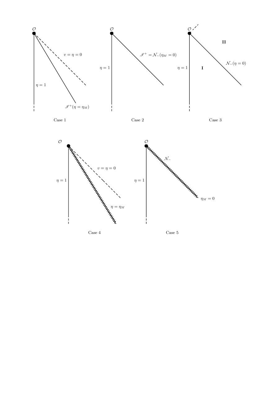
Figure 1: Possible structures of the spacetime. Case 3 depicts the spacetimes corresponding to values $(k^{2},V_{0},l_{0})\in K)$, which are the subject of this paper. The remaining cases are various other subcases. $u,v$ are respectively retarded and advanced null coordinates and $\eta=v/u$.

We note that the spacetimes which have a singularity at $\eta=\eta_{M}\in[0,1)$ are singular at all times: there is no spacelike slice $\Sigma$ which avoids the singularity. Thus there is no spacelike slice along which we can impose initial data for the Einstein equations, and so this class of spacetimes is not relevant to the issue of cosmic censorship.
For $(k^{2},V_{0},l_{0})\in K$, where $K$ is the complement in $(0,+\infty)\times\mathbb{R}^{2}$ of $\bar{K}$, it was shown that $\mathcal{N}_{-}$ is a regular surface that exists as part of the spacetime and the solutions may be extended into the region beyond $\mathcal{N}_{-}$. This is Case 3 in Figure 1. We define region II as the region bounded by $\mathcal{N}_{-}$ and the (putative) future null cone of the origin, $\mathcal{N}_{+}$. Our aim is to obtain the global structure of these solutions in this region and determine whether $\mathcal{N}_{+}$ exists as part of the spacetime. In other words, we seek to determine whether or not the singularity $\cal{O}$ is naked. In Section 2 we give a summary of the formulation of the field equations from [1] and cast them as a dynamical system in a new set of variables. In Section 3 we give the asymptotic behaviour of solutions at $\mathcal{N}_{-}$, which is a fixed point of the dynamical system, and corresponds to the limit $t\rightarrow-\infty$, where $t$ is the independent variable. Section 4 contains an analysis of the remaining fixed points which are possible end states of solutions which reach the surface ${\cal N}_{+}$. We then determine the global behaviour of solutions in Section 5 and show that, for all solutions, the maximal interval of existence is bounded above.
The main result of the paper is established in Section 6. We quote the relevant theorem here:

Theorem 1.1.

The class of spacetimes with line element (7), subject to the Einstein-Scalar Field equations (10) with $(k^{2},V_{0},l_{0})\in K$ and the regular axis conditions (10) satisfy strong cosmic censorship: the spacetimes are globally hyperbolic and $C^{1}$-inextendible.

To prove this theorem, we present a number of results giving the global structure of the spacetimes, showing that the spacetimes are globally hyperbolic. To prove $C^{1}$-inextendibility, we show that a certain invariant of the spacetime, which depends only on the metric and its first derivatives, blows up at the spacelike singularity. Two cases arise; in the first case, this spacelike hypersurface corresponds to a scalar curvature singularity and in the second case it corresponds to a non-regular axis. $C^{1}$-inextendibility holds in both cases.

Before proceeding to the technicalities leading up to the proof of Theorem 1.1, we make some general comments. Theorem 1.1, which builds on the results of Paper I, establishes that strong cosmic censorship holds for cylindrical spacetimes coupled to non-minimally coupled scalar fields in the case of self-similarity. Thus it provides a partial extension of the results of [3]: we note that the non-minimally coupled scalar field does not satisfy the energy conditions required in [3].

Self-similarity forces the potential of the non-minimally coupled scalar field to assume an exponential form (see e.g. [4] and [5] for a detailed proof). In spherical symmetry, non-minimally coupled scalar fields have been considered in [6] and [7]. Dafermos established that when the potential is bounded below by a constant (which can be negative), certain types of singularity are ruled out. Furthermore, weak cosmic censorship follows if the existence of a single trapped surface can be established [7]. In the present case, this condition on the potential corresponds to $V_{0}>0$ (see equation (8) below). However, our strong cosmic censorship result also holds when $V_{0}<0$. Thus it would be of interest to see if the results of the present paper extend to the spherically symmetric case, with and without the assumption of self-similarity.

Scalar fields with an exponential potential have also been discussed extensively in the context of cosmology, where the role of the potential as a driver of inflation and accelerated expansion is of particular note. Homogeneous and isotropic models were first considered in [8] and there is now a significant body of literature on these models. Of particular note are the deep results on nonlinear stability, in the absence of symmetries, obtained in [9] and [10].

2 Self-similar cylindrically symmetric spacetimes coupled to a non-linear scalar field

We consider cylindrically symmetric spacetimes with whole-cylinder symmetry [11] (see also [12, 13]). This class of spacetimes admits a pair of commuting, spatial Killing vectors $\boldsymbol{\xi}_{(\theta)}$, $\boldsymbol{\xi}_{(z)}$ called the axial and translational Killing vectors, respectively. Introducing double null coordinates $(u,v)$ on the Lorentzian 2-spaces orthogonal to the surfaces of cylindrical symmetry, the line element may be written as:

$$ds^{2}=-2e^{2\bar{\gamma}+2\bar{\phi}}dudv+e^{2\bar{\phi}}r^{2}d\theta^{2}+e^{-2\bar{\phi}}dz^{2},$$ (1)

where $r$ is the radius of cylinders, $\bar{\gamma},\bar{\phi}$ and $r$ depend on $u$ and $v$ only.
We take the matter source to be a cylindrically symmetric, self-interacting scalar field $\psi(u,v)$ with stress-energy tensor given by

$$T_{ab}=\nabla_{a}\psi\nabla_{b}\psi-\frac{1}{2}g_{ab}\nabla^{c}\psi\nabla_{c}\psi-g_{ab}V(\psi),$$ (2)

where $V(\psi)$ is the scalar field potential. The minimally coupled case $V\equiv 0$ was dealt with in [1] and so we assume $V\neq 0$. The line element is preserved by the coordinate transformations

$$u\rightarrow\bar{u}(u),\quad v\rightarrow\bar{v}(v),\quad z\rightarrow\lambda z,$$ (3)

for constant $\lambda$. Note that $\theta\in[0,2\pi)$ and so transformations of the kind $\theta\rightarrow\lambda\theta$ are not allowed in general. We assume self-similarity of the first kind [2], which is equivalent to the existence of a homothetic Killing vector field $\boldsymbol{\xi}$ such that

$$\mathcal{L}_{\boldsymbol{\xi}}g_{\mu\nu}=2g_{\mu\nu},$$ (4)

where $\mathcal{L}_{\boldsymbol{\xi}}$ denotes the Lie derivative along the vector $\boldsymbol{\xi}$. We make the further assumption that $\boldsymbol{\xi}$ is cylindrical. The limitations of this assumption are discussed in [1]. Equation (4) gives the form $\boldsymbol{\xi}=\alpha(u)\partial_{u}+\beta(v)\partial_{v}$ and the coordinate freedom (3) is used to set $\alpha(u)=2u,\beta(v)=2v$. Equations (4) then lead to

$$\bar{\gamma}=\gamma(\eta),\qquad\bar{\phi}=\phi(\eta)-\log|u|^{1/2},\qquad r=|u|S(\eta),$$ (5)

where

$$\eta=\frac{v}{u}$$ (6)

is called the similarity variable. The self-similar line element is then given by

$$ds^{2}=-2|u|^{-1}e^{2\gamma(\eta)+2\phi(\eta)}dudv+|u|e^{2\phi(\eta)}S^{2}(\eta)d\theta^{2}+|u|e^{-2\phi(\eta)}dz^{2}.$$ (7)

It was shown in [1] that in this coordinate system the self-similar, non-minimally coupled scalar field and its potential have the form

$$\psi=\frac{k}{2}\left(l(\eta)+\log|u||\eta|^{1/2}\right),\qquad V(\psi)=\frac{\bar{V}_{0}e^{-l(\eta)}}{|u||\eta|^{1/2}},$$ (8)

for a function $l$ and constants $\bar{V}_{0}\neq 0,k\neq 0$. The field equations then reduce to (see [1])

$$2\gamma+2\phi=\frac{k^{2}l}{2}-\frac{1}{2}\log|\eta|+c_{1},$$ (9a)

$$\eta S^{\prime\prime}=-V_{0}|\eta|^{-1}e^{\lambda l}S,$$ (9b)

$$2S^{\prime}\gamma^{\prime}-S^{\prime\prime}-2S\phi^{\prime 2}=\frac{k^{2}S}{4}\left(l^{\prime}+\frac{1}{2\eta}\right)^{2}$$ (9c)

$$2S\phi^{\prime}+S^{\prime}=-|\eta|^{-1/2},$$ (9d)

$$\eta Sl^{\prime\prime}+\eta S^{\prime}l^{\prime}+\frac{Sl^{\prime}}{2}-\frac{S}{4\eta}=-\frac{2V_{0}}{k^{2}|\eta|}Se^{\lambda l},$$ (9e)

where $V_{0}=e^{c_{1}}\bar{V_{0}}$ is constant and $\lambda=k^{2}/2-1$. Equation (9e) is the wave equation for $\psi$ and is obtained from $\nabla^{a}\nabla_{a}\psi-V^{\prime}(\psi)=0$. Region I of the spacetime corresponds to the interval $\eta\in[0,1]$, with the axis at $\eta=1$ and $\cal{N}_{-}$ at $\eta=0$. The regular axis conditions for the metric functions were found to be [1]

$$S(1)=0,\quad S^{\prime}(1)=-1,\quad\gamma^{\prime}(1)=0,\quad\phi^{\prime}(1)=-1/4.$$ (10)

For values $(k^{2},V_{0},l_{0})\in K$, solutions exist throughout region I, and $\cal{N}_{-}$ is a regular spacetime hypersurface. These solutions, which are the subject of this paper, may be extended into region II, which corresponds to $\eta\in(-\infty,0]$. It is assumed that $(k^{2},V_{0},l_{0})\in K$ for the remainder of the paper. Notice that, in particular, we have $k^{2}<2$, or equivalently $\lambda<0$ and $|\lambda|=1-k^{2}/2<1$. Note that $\cal{N_{-}}$ is at $\eta=0$ and $\cal{N}_{+}$ is at $u=0,v\in[0,\infty)$. Hence, $\eta\rightarrow-\infty$ everywhere on $\cal{N}_{+}$, approaching from inside region II. For the remainder of this paper, when we take the limit $\eta\rightarrow-\infty$, it is implied that we are taking the limit $u\rightarrow 0$ along lines of constant $v>0$. Our aim is to determine whether or not $\mathcal{N}_{+}$ exists as part of the spacetime, which answers the question of whether the singularity is naked or not. This coordinate layout is illustrated in Figure 2. We work with a rescaling of the similarity variable, which replaces (10) with an autonomous system, and adopt a dynamical systems approach.

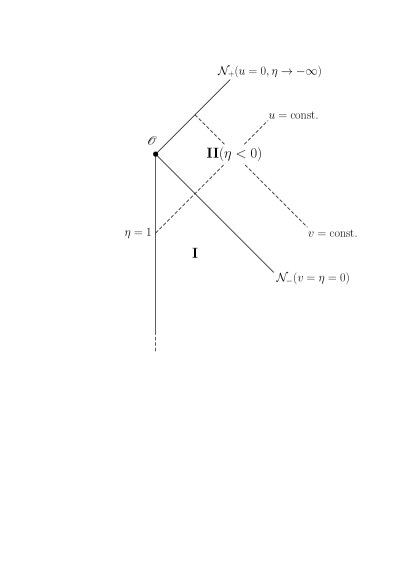
Figure 2: Coordinate layout. Our central question is whether or not ${\cal{N}}_{+}$ is part of the spacetime.

Proposition 2.1.

Let $t=\log(-\eta),\delta={\rm sgn}(V_{0}),\sigma(t)=S(\eta)$ and

$$x_{0}(t)=\frac{e^{t/2}}{\sigma(t)},\qquad x_{1}(t)=\frac{\eta S^{\prime}(\eta)}{S}=\frac{\sigma^{\prime}(t)}{\sigma(t)},$$ (11)

$$x_{2}(t)=|V_{0}|e^{\lambda l(\eta)},\qquad x_{3}(t)=\eta l^{\prime}(\eta)+\frac{1}{2}=\frac{dl}{dt}+\frac{1}{2}.$$

Then $x_{0},x_{1},x_{2},x_{3}$ satisfy

$$x_{1}^{\prime}(t) =x_{1}+\delta x_{2}-x_{1}^{2},$$ (12a)

$$x_{2}^{\prime}(t) =|\lambda|\left(\frac{1}{2}-x_{3}\right)x_{2},$$ (12b)

$$x_{3}^{\prime}(t) =\frac{x_{3}}{2}+\frac{x_{1}}{2}+\delta\frac{2x_{2}}{k^{2}}-x_{1}x_{3},$$ (12c)

$$x_{1}^{2}- x_{0}^{2}-\left(\frac{k^{2}}{2}+1\right)x_{1}-\frac{k^{2}x_{3}^{2}}{2}+k^{2}x_{1}x_{3}-2\delta x_{2}=0,$$ (12d)

$$\lim_{t\rightarrow-\infty}(x_{0},x_{1},x_{2},x_{3})=(0,0,0,0).$$ (12e)

Proof.

First note that (12b) comes directly from the definitions of $x_{2}$ and $x_{3}$. Given $f(\eta)$, defining $F(t)=f(\eta)$ yields $\eta f^{\prime}(\eta)=F^{\prime}(t)$ and $\eta^{2}f^{\prime\prime}(\eta)=F^{\prime\prime}(t)-F^{\prime}(t)$. Equations (12a) and (12c) follow directly from (9b) and (9e). Equation (9d) is equivalent to

$$\frac{d\phi}{dt}=\frac{x_{0}-x_{1}}{2}.$$ (13)

Differentiating (9a) with respect to $t$ gives

$$2\frac{d\gamma}{dt}=-2\frac{d\phi}{dt}+\frac{k^{2}}{2}\frac{dl}{dt}-\frac{1}{2}=x_{1}-x_{0}+\frac{k^{2}x_{3}}{2}-\frac{k^{2}}{4}-\frac{1}{2}.$$ (14)

Dividing (9c) by $S$, changing variables and replacing $d\gamma/dt$ and $d\phi/dt$ using (13) and (14) produces

$$x_{1}\left(x_{1}-x_{0}+\frac{k^{2}x_{3}}{2}-\frac{k^{2}}{4}-\frac{1}{2}\right)-\delta x_{2}-\frac{1}{2}\left(x_{0}-x_{1}\right)^{2}=\frac{k^{2}x_{3}^{2}}{4}.$$ (15)

Multiplying by 2 and simplifying gives (12d). It was shown in [1] that

$$\lim_{\eta\rightarrow 0+}\left(\eta l^{\prime}(\eta),|V_{0}|e^{\lambda l},\frac{\eta S^{\prime}(\eta)}{S}\right)=\left(-\frac{1}{2},0,0\right),$$ (16)

and that $S$ is non-zero and finite at $\eta=0$. The condition (12e) follows immediately. ∎

We note that the equations (12a)-(12c) subject to (12e) define a dynamical system and may be studied independently of (12d).

3 Asymptotic behaviour of solutions at $\mathcal{N}_{-}$

Proposition 3.1.

Let

$$\mu_{1}=x_{1}+Ax_{2},\qquad\mu_{3}=x_{3}+Bx_{2},$$ (17a)

$$A=\delta\frac{4}{2+k^{2}},\qquad B=\delta\frac{16}{k^{4}(2+k^{2})}.$$ (17b)

Then $$\mu_{1},\mu_{3}$$ satisfy

$$\mu_{1}^{\prime}=\mu_{1}-x_{1}^{2}-A|\lambda|x_{2}x_{3},$$ (17c)

$$\mu_{3}^{\prime}=\frac{\mu_{3}}{2}+\frac{\mu_{1}}{2}-x_{1}x_{3}-B|\lambda|x_{2}x_{3}.$$ (17d)

Proof.

It is straightforward to check that (17c),(17d) follow directly from (17a),(17b) and (12a)-(12c). ∎

We make use of the following result, which may be found in chapter 9 of [14].

Theorem 3.1.

In the differential equation

$${\boldsymbol{x}}^{\prime}(t)=F{\boldsymbol{x}}+G({\boldsymbol{x}}),$$ (18)

let $G(\boldsymbol{x})$ be of class $C^{1}$ with $G(0)=0,\partial_{\boldsymbol{x}}G(0)=0$. Let the constant matrix $F$ possess $d>0$ eigenvalues having positive real parts, say, $d_{i}$ eigenvalues with real parts equal to $\alpha_{i}$, where $\alpha_{1}>\ldots>\alpha_{r}>0$ and $d_{1}+\ldots+d_{r}=d,$ whereas the other eigenvalues, if any, have non-positive real parts. If $0<\omega<\alpha_{r},$ then (18) has solutions ${\boldsymbol{x}=\boldsymbol{x}}(t)$$\neq 0$, satisfying

$$||{\boldsymbol{x}}(t)||e^{-\omega t}\to 0,\qquad\mbox{as}\qquad t\rightarrow-\infty,$$ (19)

where $||{\boldsymbol{x}}(t)||$ denotes the Euclidean norm, and any such solution satisfies

$$\lim_{t\rightarrow-\infty}t^{-1}\log||{\boldsymbol{x}}(t)||=\alpha_{i},\qquad\mbox{for some }i.$$ (20)

$\square$
We define the vector $\boldsymbol{x}$ by

$$\boldsymbol{x}=(x_{1},x_{2},x_{3}).$$ (21)

The system defined by (12a)-(12c) and (12e) satisfies the hypothesis of this theorem, which grants local existence of solutions near the origin of the $\boldsymbol{x}$-system, which is at $t=-\infty$. We denote by $(-\infty,t_{M})$ the maximal interval of existence for a given solution.

Lemma 3.1.

For any $\epsilon>0$, there exists $T(\epsilon)\in(-\infty,t_{M})$ such that

$$|x_{i}|<e^{(|\lambda|/2-\epsilon)t},$$ (22)

for $t<T(\epsilon)$ and each $i\in\{1,2,3\}$.

Proof.

The system defined by (12a)-(12c) is of the form (18), where the matrix

$$F=\left(\begin{array}[]{ccc}1&\delta&0\\ 0&|\lambda|/{2}&0\\ 1/{2}&{2\delta}/{k^{2}}&{1}/{2}\end{array}\right)$$ (23)

has 3 positive eigenvalues, $|\lambda|/2,1/2$ and $1$, of which $|\lambda|/2$ is the smallest. Solutions to (12a)-(12c) therefore exist, which satisfy (19) and (20). Using (20), for any $\epsilon>0$, there exists $T(\epsilon)<0$ such that

$$\log||\boldsymbol{x}(t)||<(|\lambda|/2-\epsilon)t,$$ (24)

for all $t<T(\epsilon)$. Since $|x_{i}|\leq||\boldsymbol{x}||$ for each $i\in\{1,2,3\}$, the result follows. ∎

Lemma 3.2.

For $\delta=1\,(\mbox{\emph{respectively}}\,\delta=-1)$, there exists $T\in(-\infty,t_{M})$ such that $x_{1}<0,x_{3}<0\,(\mbox{\emph{respectively}}\,x_{1}>0,x_{3}>0)$ for $t\in(-\infty,T)$.

Proof.

Using Lemma 3.1 we have $|x_{i}|=O(e^{(|\lambda|/2-\epsilon)t})$ in the limit $t\rightarrow-\infty$, for any $\epsilon>0$. From (17c) we then have

$$\frac{d}{dt}\left(e^{-t}\mu_{1}\right)=-e^{-t}(x_{1}^{2}+A|\lambda|x_{2}x_{3})=O(e^{(|\lambda|-2\epsilon-1)t})\quad\mbox{as}\quad t\rightarrow-\infty,$$ (25)

which may be integrated to give

$$\mu_{1}=c_{2}e^{t}+O(e^{(|\lambda|-2\epsilon)t})=O(e^{(|\lambda|-2\epsilon)t}),$$ (26)

and so

$$x_{1}=-Ax_{2}+O(e^{(|\lambda|-2\epsilon)t})\quad\mbox{as}\quad t\rightarrow-\infty,$$ (27)

for some constant $c_{2}$, by choosing $\epsilon>0$ so that $|\lambda|-2\epsilon<1$ (recall that $|\lambda|<1$). A similar process using (17d) yields

$$\mu_{3}=O(e^{mt}),$$ (28)

and so

$$x_{3}=-Bx_{2}+O(e^{mt})\quad\mbox{as}\quad t\rightarrow-\infty,$$ (29)

where $m=\min\{1/2,|\lambda|-2\epsilon\}$. Since $\lim_{t\rightarrow-\infty}x_{3}=0$, we may choose $T(\epsilon)$ such that $|\lambda x_{3}|<\epsilon$ for $t<T(\epsilon)$. We then have

$$\frac{x_{2}^{\prime}}{x_{2}}<\frac{|\lambda|}{2}+\epsilon,\qquad\mbox{for }t\in(-\infty,T(\epsilon)).$$

Integrating over $[t,T]$ shows that $x_{2}(t)>x_{2}(T)e^{(|\lambda|/2+\epsilon)(t-T)}$ on the same interval. Choosing $\epsilon$ such that $|\lambda|/2+\epsilon<\min\{1/2,|\lambda|-2\epsilon\}$ shows that the $x_{2}$ terms in equations (27) and (29) are dominant for $t$ sufficiently close to $-\infty$. $T$ may be then chosen, without loss of generality, such that $x_{1}$ and $x_{3}$ have the same sign as $-Ax_{2}$ and $-Bx_{2}$ on $(-\infty,T)$, respectively. Note from (17b) that $A$ and $B$ have the same sign as $\delta$. ∎

Proposition 3.2.

There exists $c_{3}>0$ such that

$$\lim_{t\rightarrow-\infty}e^{-|\lambda|t/2}{\boldsymbol{x}}=c_{3}\left(A,1,B\right).$$ (30)

Proof.

Integrating (12b) over $[t,T]$ we have

$$e^{-|\lambda|t/2}x_{2}(t)=e^{-|\lambda|T/2}x_{2}(T)+\int_{t}^{T}e^{-|\lambda|t^{\prime}/2}|\lambda|x_{2}x_{3}\,dt^{\prime}.$$ (31)

Consider the case $\delta=-1$. By Lemma 3.2 we have $x_{3}>0$ on $t\in(-\infty,T)$, and by choosing $T$ sufficiently small such that the bounds of Lemma 3.1 hold, we have

$$e^{-|\lambda|T/2}x_{2}(T)<e^{-|\lambda|t/2}x_{2}(t)<e^{-|\lambda|T/2}x_{2}(T)+\int_{t}^{T}|\lambda|e^{(|\lambda|/2-2\epsilon)t^{\prime}}\,dt^{\prime}.$$ (32)

The integral here is finite in the limit $t\rightarrow-\infty$ for $\epsilon<|\lambda|/4$ and so $e^{-|\lambda|t/2}x_{2}$ has positive and finite upper and lower bounds in the limit as $t\rightarrow-\infty$. It is also monotone for $t<T$ and so we have $\lim_{t\rightarrow-\infty}e^{-|\lambda|t/2}x_{2}=c_{3}>0$, for some $c_{3}>0$. A similar argument gives this result in the case $\delta=1$. Multiplying (27) and (29) by $e^{-|\lambda|t/2}$ and taking the limit $t\rightarrow-\infty$ gives $\lim_{t\rightarrow-\infty}e^{-|\lambda|t/2}\boldsymbol{x}=c_{3}(A,1,B)$. ∎

Comment 3.1. For convenience, we define $t_{*}$ by $c_{3}=e^{-|\lambda|t_{*}/2}$. Notice then that the result of 3.2 may be written as $\lim_{\bar{t}\rightarrow-\infty}e^{-|\lambda|\bar{t}/2}{\boldsymbol{x}}=\left(A,1,B\right)$ where $\bar{t}=t-t_{*}$. Noting that (12a)-(12c) is invariant under translations of the independent variable we drop the bar and let $\bar{t}=t$. Hence

$$\lim_{t\rightarrow-\infty}e^{-|\lambda|t/2}{\boldsymbol{x}}=\left(A,1,B\right).$$ (33)

This describes the asymptotic behaviour of solutions to the future of $\cal{N}_{-}$, as they emerge from $\cal{N}_{-}$.

4 Analysis of fixed points

Proposition 4.1.

The equilibrium points of the system (12a)-(12c) are given by

$$P_{1}=(1,0,1),\quad P_{2}=\left(\alpha_{-},\frac{-\delta k^{2}}{8},\frac{1}{2}\right),\quad P_{3}=\left(\alpha_{+},\frac{-\delta k^{2}}{8},\frac{1}{2}\right),$$ (34)

where

$$\alpha_{\pm}=\frac{1\pm\sqrt{|\lambda|}}{2}.$$ (35)

Proof.

This is straightforward to check. ∎

Proposition 4.2.

Define $f(\boldsymbol{x})$ by setting ${\boldsymbol{x}}^{\prime}(t)=f({\boldsymbol{x}})$, where the component equations are given by (12a)-(12c). Let

$${\boldsymbol{y}}(s)=(y_{1},y_{2},y_{3}),\qquad\begin{array}[]{ll}y_{1}(s)=1-x_{1}(t)\\ y_{2}(s)=x_{2}(t)\\ y_{3}(s)=1-x_{3}(t)\end{array}\qquad s=-t.$$ (36)

Then

$${\boldsymbol{y}}^{\prime}(s)=f({\boldsymbol{y}}).$$ (37)

Proof.

This is straightforward to check. ∎

Proposition 4.3.

Suppose $\lim_{t\rightarrow\infty}{\boldsymbol{x}}=P_{1}$. Then

$$\lim_{t\rightarrow\infty}e^{|\lambda|t/2}(1-x_{1},x_{2},1-x_{3})=c(A,1,B),$$ (38)

for some constant $c>0$.

Proof.

First note that $\lim_{t\rightarrow\infty}\boldsymbol{x}=P_{1}$ is equivalent to $\lim_{s\rightarrow-\infty}\boldsymbol{y}=(0,0,0)$. Since $\boldsymbol{y}^{\prime}(s)=F(\boldsymbol{y})$, solutions emanating from the origin of the $y$-system satisfy the exact conditions satisfied by solutions emanating from the origin of the $x$-system used in the proofs of Section 3. We may, therefore, carry out an identical analysis to find

$$\lim_{s\rightarrow-\infty}e^{-|\lambda|s/2}\boldsymbol{y}=c(A,1,B),$$ (39)

which is our result. ∎

Proposition 4.4.

Let $k^{2}<2$ with $k^{2}\neq\sqrt{3}-1$. Suppose that $\lim_{t\rightarrow\infty}{\boldsymbol{x}}=P_{1}$. Then $\lim_{t\rightarrow\infty}r$ is non-zero and finite and $\mathcal{R}$ is bounded in this limit, where $\cal{R}$ is the Ricci scalar corresponding to the line element (7) and $r=|u|\sigma$ is the radius of the cylinders in this spacetime.

Proof.

Using Proposition 4.3, for any $\epsilon>0$ there exists $T(\epsilon)$ such that

$$1-(Ac+\epsilon)e^{-|\lambda|t/2}<x_{1}<1-(Ac-\epsilon)e^{-|\lambda|t/2},$$ (40)

for $t>T(\epsilon)$. Recalling $x_{1}=\sigma^{\prime}/\sigma$, it is straightforward to show that this leads to

$$C_{1}<e^{-t}\sigma<C_{2},\qquad t>T(\epsilon),$$ (41)

for positive constants $C_{1},C_{2}$. We also have

$$\frac{d}{dt}(e^{-t}\sigma)=e^{-t}\sigma\left(x_{1}-1\right).$$ (42)

Using (40) shows that $e^{-t}\sigma$ is monotone decreasing near $P_{1}$. Moreover, this may be integrated using (40) to show that $e^{-t}\sigma$ has a finite, non-zero limit as $t\rightarrow\infty$. In region II of the spacetime we have $v>0,u<0$ and thus $|u|=-v/\eta=ve^{-t}$. It follows that $r=|u|\sigma=ve^{-t}\sigma$ has a positive finite limit approaching ${\cal{N}}_{+}\,(u=0)$ along lines of constant $v$. It follows from (13),(40) and (41) that

$$\frac{1}{C_{2}e^{t/2}}+(Ac-\epsilon)e^{-|\lambda|t/2}<2\frac{d\phi}{dt}+1<\frac{1}{C_{1}e^{t/2}}+(Ac+\epsilon)e^{-|\lambda|t/2},$$ (43)

for $t>T(\epsilon)$. We see that if $\epsilon\leq Ac$ then $2\phi+t$ is monotone in $t$. Integrating and taking exponentials then shows that $\lim_{t\rightarrow\infty}e^{2\phi+t}$ exists, is non-zero and finite. Hence, $\lim_{t\rightarrow\infty}|u|e^{-2\phi}=\lim_{t\rightarrow\infty}ve^{-2\phi-t}$ is non-zero and finite. So far we have shown that $g_{\theta\theta}=|u|^{-1}e^{2\phi}r^{2}$ and $g_{zz}=|u|e^{-2\phi}$ have non-zero, finite limits as $t\rightarrow+\infty$. Using similar arguments, it may shown that the metric component $|u|^{-1}e^{2\gamma+2\phi}$ behaves like $e^{(1-|\lambda|/2)t}$ in the limit as $t\rightarrow+\infty$ and, therefore, has limit $+\infty$. However, by making the coordinate transformation $\bar{u}=-2|u|^{|\lambda|/2}/|\lambda|$ we avoid this problem. The corresponding metric component in this coordinate system is $|\bar{u}|^{-1}e^{2\gamma+2\phi}$ and it may be shown in a similar fashion that this has a non-zero, finite limit as $t\rightarrow+\infty$. In [1] it was shown that the Ricci scalar may be written as

$$\mathcal{R}=\frac{e^{-k^{2}l/2+t/2-c_{1}}}{v}\left(\frac{k^{2}}{2}\left(1-x_{3}\right)x_{3}-4\delta x_{2}\right).$$ (44)

It may be shown, using (38) in a similar way, that for all sufficiently large $t$, we have

$$C_{3}e^{|\lambda|t/2}<e^{-k^{2}l/2+t/2-c_{1}}<C_{4}e^{|\lambda|t/2},$$ (45)

for some positive constants $C_{3},C_{4}$. (To obtain this result, we integrate the third component of the vector in (38) at large $t$ to obtain

$$e^{c_{1}}\exp[O(e^{\lambda t/2})]<e^{-(l-t/2)}<e^{c_{2}}\exp[O(e^{\lambda t/2})]$$ (46)

and combine with the second component of (38).) We also have

$$\lim_{t\rightarrow\infty}e^{|\lambda|t/2}\left(\frac{k^{2}}{2}\left(1-x_{3}\right)x_{3}-4\delta x_{2}\right) =\frac{k^{2}Bc}{2}-4\delta c$$

$$=\left(\frac{8}{k^{2}(2+k^{2})}-4\right)\delta c\neq 0,$$

for $k^{2}\neq\sqrt{3}-1$, using (38). Combining this with (44) and (45) shows that $\lim_{t\rightarrow\infty}\mathcal{R}$ is bounded for essentially all $k^{2}<2$. ∎

This result shows that in spacetimes where the solutions to the field equations satisfy $\lim_{t\rightarrow\infty}\boldsymbol{x}=P_{1}$, the future null cone of the singularity $\cal{N}_{+}$ is regular and exists are part of the spacetime, thus rendering the singularity at the origin naked. However, it is shown in later sections that none of the solutions actually do evolve to $P_{1}$.

Proposition 4.5.

If $\lim_{t\rightarrow\infty}{\boldsymbol{x}}=P_{2}$ or $\lim_{t\rightarrow\infty}{\boldsymbol{x}}=P_{3}$, then $\lim_{t\rightarrow\infty}r=0$ and $\lim_{t\rightarrow\infty}\mathcal{R}=+\infty$, where $r$ is the radius of the cylinders and $\mathcal{R}$ is the Ricci scalar.

Proof.

If $\lim_{t\rightarrow\infty}x_{1}=\alpha_{\pm}$ then for any $\epsilon>0$ there exists $T(\epsilon)$ such that $x_{1}<\alpha_{+}+\epsilon$ for $t>T(\epsilon)$, since $\alpha_{-}<\alpha_{+}$. Note that $\sqrt{|\lambda|}=\sqrt{1-k^{2}/2}<1-k^{2}/4$, which gives $\alpha_{+}<1-k^{2}/8$. This leads to $\sigma<\sigma(T)e^{(1-k^{2}/8+\epsilon)(t-T)}$ for $t>T$. It follows that $r=|u|\sigma<v\sigma(T)e^{(-k^{2}/8+\epsilon)(t-T)}$ for $t>T$. Choosing $\epsilon<k^{2}/8$ shows that $\lim_{t\rightarrow\infty}r=0$, for $v\in(0,\infty)$. It is straightforward to show that $\lim_{t\rightarrow\infty}e^{-k^{2}l/2+t/2}=+\infty$ follows from $\lim_{t\rightarrow\infty}dl/dt=0$, which is equivalent to $\lim_{t\rightarrow\infty}x_{3}=1/2$. Then using $\lim_{t\rightarrow\infty}x_{2}=k^{2}/8$ and $\delta=-1$ we find that $\lim_{t\rightarrow\infty}\mathcal{R}=+\infty$. ∎

Proposition 4.6.

Let $\delta=-1$. Then there is no solution of (12a)-(12d) which satisfies $\lim_{t\rightarrow\infty}\boldsymbol{x}=P_{2}$.

Proof.

$x_{0}$ satisfies

$$x_{0}^{\prime}=x_{0}\left(\frac{1}{2}-x_{1}\right).$$ (48)

If $\lim_{t\rightarrow\infty}x_{1}=1/2-\sqrt{|\lambda|}/2$ then $x_{0}^{\prime}\sim(\sqrt{|\lambda|}/2)x_{0}$ as $t\rightarrow+\infty$. Since $x_{0}>0$ for $t>-\infty$ we must have $\lim_{t\rightarrow\infty}x_{0}=+\infty$. This contradicts $\lim\boldsymbol{x}=P_{2}$ and (12d). ∎

Proposition 4.7.

Let $\delta=+1$. Then there is no solution of (12a)-(12d) which satisfies $\lim_{t\rightarrow\infty}\boldsymbol{x}=P_{2}$ or $\lim_{t\rightarrow\infty}\boldsymbol{x}=P_{3}$.

Proof.

This follows immediately from the fact that $x_{2}>0$. ∎

Comment 4.1 We note that $\lim_{t\rightarrow t_{M}^{-}}\boldsymbol{x}=P_{1}$ or $P_{3}$ are consistent with (12d).

5 Global behaviour of solutions of the dynamical system

Our aim in this section is to give a complete account of the future evolution of solutions of the dynamical system (12a)-(12e) in the case $\lambda<0$ (corresponding to Case 3 in Figure 1). Our conclusion, given in Propositions 5.1 and 5.2 below, is that in every case, the maximal interval of existence is bounded above: the solutions only exist for a finite time in the future. We note that as the solutions evolve from $t=-\infty$, the maximal interval of existence must have the form $(-\infty,t_{M})$ for some $t_{M}\leq+\infty$. The key conclusion that we make is that $t_{M}$ is finite in every case.

The argument is structured as follows. The first important result is Lemma 5.2, where we deduce that the state variables $x_{i}$, $i=1,2,3$ are monotone in a neighbourhood of $t=t_{M}$. This requires Lemma 5.1. In Lemmas 5.3 - 5.6, we establish connections between the limits of various state variables as $t\to t_{M}$. Lemmas 5.7 - 5.11 are linked by the theme of finding precursors to $t_{M}$ being finite. Among these is the important Lemma 5.8 which provides restrictions on possible limits of some of the key state variables as $t\to t_{M}$. Propositions 5.1 and 5.2 then establish our main result, that $t_{M}$ is indeed finite.

To begin, we quote the following standard result which is helpful in determining the maximal intervals of existence (see, for example, [15], ch.4).

Theorem 5.1.

Let $\Psi_{\boldsymbol{a}}(t)$ be the unique solution of the differential equation ${\boldsymbol{x}}^{\prime}={\boldsymbol{f}(\boldsymbol{x})}$, where ${\boldsymbol{f}}\in C^{1}(\mathbb{R}^{n})$, which satisfies ${\boldsymbol{x}}(0)={\boldsymbol{a}}$, and let $(t_{\min},t_{\max})$ be the maximal interval of existence on which $\Psi_{\boldsymbol{a}}(t)$ is defined. If $t_{\max}$ is finite, then

$$\lim_{t\rightarrow t^{-}_{\max}}||\Psi_{\boldsymbol{a}}(t)||=+\infty.$$ (49)

This theorem tells us that solutions exist while each component of the solution is finite. Recall that our maximal interval of existence has the form $(t_{\min},t_{\max})=(-\infty,t_{M})$.

Lemma 5.1.

For $V_{0}<0$ (so that $\delta=-1$), suppose there exists $t_{0}\in(-\infty,t_{M})$ such that $x_{3}(t_{0})=1/2$ and $x_{3}<1/2$ for $t\in(-\infty,t_{0})$. Then $x_{2}(t_{0})<k^{2}/8$ and $x_{3}(t)>1/2$, $x_{2}(t)<k^{2}/8$ hold for all $t\in(t_{0},t_{M})$.

Proof.

First note that $x_{3}=1/2,x_{2}=k^{2}/8$ defines an invariant manifold of the system (12a)-(12c), so if $x_{3}(t_{0})=1/2$, $x_{2}(t_{0})=k^{2}/8$, then we would have $x_{3}=1/2,x_{2}=k^{2}/8$ for all $t\in(-\infty,t_{M})$, which is clearly not the case, since $x_{2},x_{3}\to 0$ as $t\to-\infty$. Moreover, at $x_{3}=1/2$ we have

$$x_{3}^{\prime}=\frac{1}{4}-\frac{2x_{2}}{k^{2}},$$ (50)

and so $x_{3}$ cannot reach $1/2$ from below if $x_{2}(t_{0})>k^{2}/8$. Hence, we must have $x_{2}(t_{0})<k^{2}/8$ and $x_{3}^{\prime}(t_{0})>0$. Equation (50) also shows that $x_{3}$ cannot cross $1/2$ from above if $x_{2}<k^{2}/8$. Given that $x_{2}$ is decreasing if $x_{3}>1/2$, we must have $x_{3}>1/2$ and $x_{2}<k^{2}/8$ for all $t\in(t_{0},t_{M})$. ∎

This leads us to an important monotonicity result:

Lemma 5.2.

Let $i\in\{1,2,3\}$. Then each $x_{i}$ is monotone in the limit as $t\rightarrow t_{M}^{-}$. Hence, either $\lim_{t\rightarrow t_{M}^{-}}x_{i}$ exists or $\lim_{t\rightarrow t_{M}^{-}}x_{i}=\pm\infty$.

Proof.

Lemma 5.1 tells us that if $\delta=-1$, then $x_{3}-1/2$ can only change sign once. If $\delta=1$, then at $x_{3}=1/2$ we have $x_{3}^{\prime}=1/4+2x_{2}/k^{2}>0$, so $x_{3}-1/2$, and thus $x_{2}^{\prime}$, can only change sign once in this case also. At $x_{1}^{\prime}=0$ we have $x_{1}^{\prime\prime}=\delta x_{2}^{\prime}$, which means that $x_{1}^{\prime}$ can only change sign twice. At $x_{1}-x_{3}=0$ we have $x_{1}^{\prime}-x_{3}^{\prime}=\delta(1-2/k^{2})x_{2}$ which always has the same sign, specifically, the opposite sign to $\delta$. Hence, $x_{1}-x_{3}$ can only change sign once also. Now, at $x_{3}^{\prime}=0$ we have

$$x_{3}^{\prime\prime}=\left(\frac{1}{2}-x_{3}\right)\left(\frac{1}{2}-x_{1}\right)\left(x_{1}-x_{3}\right).$$ (51)

The right hand side here may only change sign a finite number of times. Hence, $x_{3}^{\prime}$ eventually becomes fixed in sign and $x_{3}$ becomes monotone. ∎

Lemma 5.3.

Let $t_{0}\in(-\infty,t_{M})$ satisfy $\sigma(t_{0})\neq 0$. Then

$$\lim_{t\rightarrow t_{M}^{-}}\sigma=0\quad\Leftrightarrow\quad\lim_{t\rightarrow t_{M}^{-}}\int_{t_{0}}^{t}x_{1}\,dt^{\prime}=-\infty.$$ (52)

Furthermore, if $t_{M}<\infty$ then

$$\lim_{t\rightarrow t_{M}^{-}}\sigma=0\Rightarrow\lim_{t\rightarrow t_{M}^{-}}x_{1}=-\infty.$$ (53)

Proof.

By the definition of $x_{1}$ we have

$$\sigma=\sigma(t_{0})\exp\left(\int_{t_{0}}^{t}x_{1}\,dt^{\prime}\right),$$ (54)

from which (52) immediately follows. To establish (53) we note that since $t_{M}<\infty$, divergence of the integral $\int_{t_{0}}^{t}x_{1}\,dt^{\prime}$ as $t\to t_{M}^{-}$ implies the divergence of the integrand in this limit. ∎

Lemma 5.4.

If $t_{M}$ is finite and $\lim_{t\rightarrow t_{M}^{-}}x_{1}=-\infty$ then $\lim_{t\rightarrow t_{M}^{-}}\sigma=0$ .

Proof.

If $\lim_{t\rightarrow t_{M}^{-}}x_{1}=-\infty$ then either $\lim_{t\rightarrow t_{M}^{-}}\sigma^{\prime}=-\infty$ or $\lim_{t\rightarrow t_{M}^{-}}\sigma=0$ (see (11)). Writing (12a) in terms of $x_{2}$ and $\sigma$ gives

$$\sigma^{\prime\prime}=\sigma^{\prime}+\delta x_{2}\sigma.$$ (55)

If $\delta=1$ then we have $\sigma^{\prime\prime}>\sigma^{\prime}$, which rules out $\lim_{t\rightarrow t_{M}^{-}}\sigma^{\prime}=-\infty$, since $t_{M}$ is finite. In the case $\delta=-1$, suppose that $x_{2}$ is bounded above by a constant $b$ for all $t\in(-\infty,t_{M}]$ and let $\sigma_{M}$ be the maximum of $\sigma$ on this interval. Then we have $\sigma^{\prime\prime}>\sigma^{\prime}-b\sigma_{M}$, which also rules out $\lim_{t\rightarrow t_{M}^{-}}\sigma^{\prime}=-\infty$.

We now turn to the case $\delta=-1,\lim_{t\rightarrow t_{M}^{-}}x_{2}=+\infty$ (monotonicty, established in Lemma 5.2, leaves this as the only remaining option). Consider

$$x_{1}^{\prime}-\frac{k^{2}x_{3}^{\prime}}{2}=\frac{|\lambda|x_{1}}{2}+\left(\frac{1}{2}-x_{1}\right)\left(x_{1}-\frac{k^{2}x_{3}}{2}\right).$$ (56)

Using $e^{-t/2}\sigma$ as integrating factor we find that

$$\frac{d}{dt}\left(e^{-t/2}\sigma\left(x_{1}-\frac{k^{2}x_{3}}{2}\right)\right)=\frac{|\lambda|}{2}e^{-t/2}\sigma^{\prime}<0,$$ (57)

where the inequality holds on some interval $(t_{0},t_{M})$. Assuming $\lim_{t\rightarrow t_{M}^{-}}\sigma>0$, integrating then shows that $x_{1}-k^{2}x_{3}/2$ is bounded above for all $t\in[t_{0},t_{M}]$. We then have

$$\frac{x_{2}^{\prime}}{x_{2}}<|\lambda|\left(\frac{1}{2}+\frac{2b}{k^{2}}-\frac{2x_{1}}{k^{2}}\right),$$ (58)

for some constant $b$. Integrating shows that since $\lim_{t\rightarrow t_{M}^{-}}x_{2}=+\infty$ then $\lim_{t\rightarrow t_{M}^{-}}\int_{t_{0}}^{t}x_{1}=-\infty$, which gives $\lim_{t\rightarrow t_{M}^{-}}\sigma=0$ by Lemma 5.3. ∎

We note that Lemmas 5.3 and 5.4 tell us that, for $t_{M}<\infty$, $\lim_{t\rightarrow t_{M}^{-}}\sigma=0$ if and only if $\lim_{t\rightarrow t_{M}^{-}}x_{1}=-\infty$.

Lemma 5.5.

If $t_{M}$ is finite and $\lim_{t\rightarrow t_{M}^{-}}x_{1}=-\infty$, then $\lim_{t\rightarrow t_{M}^{-}}x_{3}=\pm\infty$ or $\lim_{t\rightarrow t_{M}^{-}}x_{3}=1/2$.

Proof.

Integrating (12c) we have

$$x_{3}=e^{(t-t_{0})/2}x_{3}(t_{0})+\int_{t_{0}}^{t}e^{(t-t^{\prime})/2}\left(\left(\frac{1}{2}-x_{3}\right)x_{1}+\delta\frac{2x_{2}}{k^{2}}\right)\,dt^{\prime},$$ (59)

for any $t_{0}\in(-\infty,t_{M})$. Given that $\lim_{t\rightarrow t_{M}^{-}}x_{1}=-\infty$, we have

$$\lim_{t\rightarrow t_{M}^{-}}\int_{t_{0}}^{t}x_{1}\,dt^{\prime}=-\infty,$$ (60)

by Lemmas 5.3 and 5.4. Assuming $|x_{3}|$ is bounded, which gives $x_{2}$ bounded by (12b), we must have $\lim_{t\rightarrow t_{M}^{-}}x_{3}=1/2$ by inspection of (59) with (60). If $x_{3}$ is unbounded then we must have $\lim_{t\rightarrow t_{M}^{-}}x_{3}=\pm\infty$ by Lemma 5.2. ∎

Lemma 5.6.

If $t_{M}$ is finite and $\lim_{t\rightarrow t_{M}^{-}}x_{3}=\pm\infty$, then $\lim_{t\rightarrow t_{M}^{-}}x_{1}=-\infty$.

Proof.

Suppose that $\lim_{t\rightarrow t_{M}^{-}}x_{3}=+\infty$. Then $\lim_{t\rightarrow t_{M}^{-}}x_{2}<\infty$, by (12b), and it follows from (12c) that $x_{3}^{\prime}<(\frac{1}{2}-x_{1})x_{3}+\frac{x_{1}}{2}+b$ for all $t\in(-\infty,t_{M})$ and some constant $b$. This yields the inequality

$$x_{3}(t)<\frac{\mu(t)}{\mu(t_{0})}x_{3}(t_{0})+\int_{t_{0}}^{t}\frac{\mu(t^{\prime})}{\mu(t)}(\frac{x_{1}}{2}+b)dt^{\prime},$$ (61)

where

$$\mu(t)=\exp\left\{\int_{t_{0}}^{t}(x_{1}-\frac{1}{2})\right\}.$$ (62)

Since $t_{M}<\infty$ we must have $\lim_{t\rightarrow t_{M}^{-}}x_{1}=-\infty$ in order that $x_{3}\to+\infty$.
Now suppose $\lim_{t\rightarrow t_{M}^{-}}x_{3}=-\infty$ and $\lim_{t\rightarrow t_{M}^{-}}x_{1}>-\infty$. Then we have $\lim_{t\rightarrow t_{M}^{-}}\sigma>0$ and it can be easily shown via (57) that $x_{1}-k^{2}x_{3}/2$ is bounded above. It follows that if $\lim_{t\rightarrow t_{M}^{-}}x_{3}=-\infty$ then $\lim_{t\rightarrow t_{M}^{-}}x_{1}=-\infty$. ∎

Lemma 5.7.

If $V_{0}<0$ (respectively $V_{0}>0$), then $x_{1}(t)<1$ (respectively $x_{1}(t)<0$) for all $t\in(-\infty,t_{M})$.

Proof.

If $\delta=-1$ then it follows directly from (12a) that $x_{1}$ cannot cross 1 from below. If $\delta=1$ then by Lemma 3.2 we have $x_{1}<0$ on an initial interval, say $(-\infty,t_{0})$. Now suppose that $x_{1}(t_{0})=0$. It is clear that $x_{0}^{\prime}>0$ on $(-\infty,t_{0})$ and so $x_{0}(t_{0})>0$. At $t_{0}$, (12d) with $\delta=1$ reduces to

$$-x_{0}^{2}(t_{0})-\frac{k^{2}x_{3}^{2}(t_{0})}{2}-2x_{2}(t_{0})=0,$$ (63)

which clearly contradicts $x_{0}(t_{0})>0$. Hence, no such $t_{0}$ exists. ∎

Lemma 5.8.

If $t_{M}$ is finite then

$$\lim_{t\rightarrow t_{M}^{-}}x_{1}=-\infty,\qquad\lim_{t\rightarrow t_{M}^{-}}\sigma=0,$$ (64)

and either

$$\lim_{t\rightarrow t_{M}^{-}}x_{3}=\pm\infty,\quad\mbox{or}\quad\lim_{t\rightarrow t_{M}^{-}}x_{3}=\frac{1}{2}.$$ (65)

Proof.

Using Theorem 5.1 and Lemma 5.2 we must have $\lim_{t\rightarrow t_{M}^{-}}|x_{i}|=+\infty$ for some $i\in\{1,2,3\}$. By (12b), if $x_{3}$ is bounded and $t_{M}$ is finite, then $x_{2}$ is bounded. By Lemma 5.7, $x_{1}<1$ for all $t\in(-\infty,t_{M})$, and so $x_{1}\to-\infty$ in this case. Alternatively, we must have $\lim_{t\to t_{M}^{-}}x_{3}=\pm\infty$ in which case $x_{1}\to-\infty$ by Lemma 5.6. Lemmas 5.4 and 5.5 complete the proof. ∎

Lemma 5.9.

For $V_{0}<0$, suppose there exists $t_{0}\in(-\infty,t_{M})$ such that $x_{1}(t_{0})<0$. Then $t_{M}$ is finite.

Proof.

If $x_{1}(t_{0})<0$ and $\delta=-1$ then (12a) yields $x_{1}^{\prime}(t_{0})<-x_{1}(t_{0})^{2}$ and so $x_{1}<0$ persists. That is, $x_{1}<0$ and $x_{1}^{\prime}<-x_{1}^{2}$ for all $t\in(t_{0},t_{M})$. Integrating shows that $x_{1}$ diverges to $-\infty$ in finite $t$. ∎

Lemma 5.10.

For $V_{0}<0$, suppose there exists $t_{0}\in(-\infty,t_{M})$ such that $x_{2}(t_{0})=k^{2}/8$ and $x_{2}<k^{2}/8$ for all $t\in(-\infty,t_{0})$. Then $x_{3}(t_{0})<1/2$ and $x_{3}<1/2$, $x_{2}>k^{2}/8$ hold for all $t\in(t_{0},t_{M})$.

Proof.

Using Lemma 5.1, we must have $x_{3}<1/2$ for all $t\in(-\infty,t_{0}]$. We also have $x_{2}^{\prime}>0$ while $x_{3}<1/2$ and since $x_{3}$ cannot cross $1/2$ from below while $x_{2}>k^{2}/8$ then we must have $x_{2}>k^{2}/8$ and $x_{3}<1/2$ for all $t\in(t_{0},t_{M})$. ∎

Lemma 5.11.

For $V_{0}<0$, suppose there exists $t_{0}\in(-\infty,t_{M})$ such that $x_{1}(t_{0})=1/2$. Then $t_{M}$ is finite.

Proof.

At $x_{1}=1/2$, equation (12d) with $\delta=-1$ simplifies to

$$\frac{1}{4}+x_{0}^{2}+\frac{k^{2}}{4}+\frac{k^{2}}{2}\left(x_{3}^{2}-x_{3}\right)=2x_{2}.$$ (66)

Using the fact the $x_{3}^{2}-x_{3}\geq-1/4$ we then have

$$x_{2}(t_{0})>\frac{1}{8}+\frac{k^{2}}{16}+\frac{x_{0}^{2}}{2}>\frac{k^{2}}{8}.$$ (67)

There must then exist $t_{*}\in(-\infty,t_{0})$ such that $x_{2}(t_{*})=k^{2}/8$ and $x_{2}(t)<k^{2}/8$ for all $t<t_{*}$. Using Lemma 5.10 we have $x_{3}<1/2$, and thus $x_{2}^{\prime}>0$, for all $t\in(t_{*},t_{M})$. Using (67) we have $x_{2}>1/8+k^{2}/16$, from which it follows that

$$x_{3}^{\prime}<\frac{\lambda}{4k^{2}}-\left(\frac{1}{2}-x_{1}\right)\left(\frac{1}{2}-x_{3}\right)<\frac{\lambda}{4k^{2}}+\frac{1}{2}\left(\frac{1}{2}-x_{3}\right)$$ (68)

for all $t\in(t_{0},t_{M})$, where we have used $x_{1}<1$ (see Lemma 5.7). This shows that $x_{3}^{\prime}<0$ if $x_{3}>1/2+\lambda/2k^{2}$. It follows that $x_{3}-1/2<m=\max\{x_{3}(t_{0})-1/2,\lambda/2k^{2}\}<0$, which gives $x_{2}^{\prime}>\lambda mx_{2}$ , for all $t\in(t_{0},t_{M})$. If $t_{M}=+\infty$ then $\lim_{t\rightarrow t_{M}^{-}}x_{2}=+\infty$ which would cause $x_{1}$ to become negative in finite $t$, contradicting Lemma 5.9. ∎

Proposition 5.1.

If $V_{0}<0$, then $t_{M}$ is finite and

$$\lim_{t\rightarrow t_{M}^{-}}x_{1}=-\infty,\qquad\lim_{t\rightarrow t_{M}^{-}}\sigma=0,$$ (69)

and either

$$\lim_{t\rightarrow t_{M}^{-}}x_{3}=\pm\infty,\quad\mbox{or}\quad\lim_{t\rightarrow t_{M}^{-}}x_{3}=\frac{1}{2}.$$ (70)

Proof.

The preceding lemma rules out the possibility that $\boldsymbol{x}$ limits to $P_{1}$ or $P_{3}$ as $t\rightarrow\infty$, since the $x_{1}$ components of $P_{1}$ and $P_{3}$ are greater than one half. Proposition 4.6 rules out the possibility that $\boldsymbol{x}$ limits to $P_{2}$. Taking note of Lemma 5.2 which rules out limit cycles and other behaviours, we see that we must either have $\lim_{t\rightarrow\infty}||\boldsymbol{x}||=+\infty$ or $t_{M}$ finite with $\lim_{t\rightarrow t_{M}^{-}}||\boldsymbol{x}||=\infty$. We may rule out the former case as follows. We can’t have $\lim_{t\rightarrow\infty}x_{1}=-\infty$, because in that case there would exist $t_{0}<+\infty$ such that $x_{1}(t_{0})<0$ and thus $t_{M}$ would be finite by Lemma 5.9. Nor can we have $\lim_{t\rightarrow\infty}x_{2}=+\infty$ since this would cause $x_{1}$ to become negative in finite $t$, via (12a), so we would have $t_{M}$ finite here also. This also rules out $\lim_{t\rightarrow\infty}x_{3}=-\infty$ since this would give $\lim_{t\rightarrow\infty}x_{2}=+\infty$, by (12b). Given that $x_{2}>0$ and $x_{1}<1$ by Lemma 5.7, this leaves the possibility that $\lim_{t\rightarrow\infty}x_{3}=+\infty$. However, it is easy to see that if $\lim_{t\rightarrow\infty}x_{3}=+\infty$ and $\lim_{t\rightarrow\infty}|x_{1}|<\infty$, then (12d) is not satisfied, since in that case we have $\lim_{t\rightarrow\infty}x_{2}<\infty$ and the left hand side has limit $-\infty$. We must, therefore, have $t_{M}$ finite. Then Lemma 5.8 applies to give the limits stated. ∎

Proposition 5.2.

If $V_{0}>0$, then $t_{M}$ is finite and

$$\lim_{t\rightarrow t_{M}^{-}}x_{1}=-\infty,\qquad\lim_{t\rightarrow t_{M}^{-}}\sigma=0,$$ (71)

and either

$$\lim_{t\rightarrow t_{M}^{-}}x_{3}=\pm\infty,\quad\mbox{or}\quad\lim_{t\rightarrow t_{M}^{-}}x_{3}=\frac{1}{2}.$$ (72)

Proof.

It is easily checked that (12d) with $\delta=1$ may be written as

$$\left(1+\frac{k^{2}}{2}\right)\left(x_{1}-x_{1}^{2}\right)=-2x_{2}-x_{0}^{2}-\frac{k^{2}}{2}\left(x_{1}-x_{3}\right)^{2},$$ (73)

from which it follows that

$$-\left(x_{1}-\frac{1}{2}\right)^{2} <-\left(\frac{x_{0}}{\kappa}\right)^{2},$$ (74)

and so

$$x_{1}-\frac{1}{2} <-\frac{x_{0}}{\kappa},$$ (75)

where $\kappa^{2}=1+k^{2}/2$ and we have used $x_{0}>0$ and $x_{1}<0$ (which is given by Lemma 5.7). This is equivalent to

$$x_{0}^{\prime}>\frac{x_{0}^{2}}{\kappa}.$$ (76)

Integrating shows that $x_{0}=e^{t/2}/\sigma$ blows up in finite time, and so $t_{M}$ is finite with $\lim_{t\rightarrow t_{M}^{-}}\sigma=0$. As in Proposition 5.1, the limits follow by Lemma 5.8. ∎

6 Global structure and strong cosmic censorship

The aim of this section is to prove a strong cosmic censorship theorem for the class of spacetimes considered here. Strong cosmic censorship is a statement about solutions of the Cauchy initial value problem in General Relativity (see p.305 of [16]). Clearly, we are not dealing with the Cauchy problem here, but the spirit of the result is the same as that of strong cosmic censorship. We prove that the solutions considered here (which evolve from a regular axis rather than an initial data surface) are globally hyperbolic and $C^{1}$-inextendible. This follows from the results established below regarding radial null geodesics, and from an argument based on the behaviour of a certain invariant $E$ of the spacetime which depends only on the metric and its first derivatives. This invariant satisfies $\lim_{t\to t_{M}^{-}}E=+\infty$, proving $C^{1}$-inextendibility. (The use here of the quantity $E$ mirrors the use of the Hawking mass to prove the $C^{1}$-inextendibility of solutions of the Einstein-Maxwell-Scalar Field equations [17].)
The quantity $E$ in question is the $C-$energy defined by Thorne [18]. In a cylindrically symmetric spacetime $(M,g)$ with axial and translational Killing vectors $\boldsymbol{\xi}_{(\theta)}$ and $\boldsymbol{\xi}_{(z)}$, the circumferential radius $\rho$, the specific length $L$ and the areal radius $r$ are defined as

$$\rho^{2}=\xi_{(\theta)a}\xi_{(\theta)}^{a},\quad L^{2}=\xi_{(z)a}\xi_{(z)}^{a},\quad r=\rho L.$$ (77)

The $C$-energy is then defined as

$$E=\frac{1}{8}\left(1-L^{-2}g^{ab}\partial_{a}r\partial_{b}r\right).$$ (78)

As noted in [13], this does not yield a uniquely defined quantity in a given cylindrical spacetime. Furthermore, $E$ can blow up even in flat spacetime. However, as we will see below, this pathology is linked to the over-abundance of Killing vector fields (KVF’s) in flat spacetime.

As we see from the definition, $E$ is not a function of the metric alone, but depends also on the KVF’s:

$$E=E(g_{ab},\boldsymbol{\xi}_{(\theta)},\boldsymbol{\xi}_{(z)}).$$ (79)

It should be more correctly understood as a function of the axis of a cylindrical spacetime, relative to a given translation along the axis. In our class of spacetimes, the axis - and corresponding KVF [19] - is given. Likewise, the definition of the class considered means that we have another KVF ($\boldsymbol{\xi}_{(z)}$) that both commutes with and is orthogonal to $\boldsymbol{\xi}_{(\theta)}$ (it is this orthogonality requirement that puts us in the class of whole cylinder symmetry). However, in a given spacetime with whole cylinder symmetry, with the axis and axial KVF specified, the translational KVF is not necessarily uniquely defined. Consequently, the $C-$energy relative to the axis is not necessarily well-defined. See [13] for a counter-example, which arises in flat spacetime. This presents a difficulty if we wish to make invariant statements about the spacetime in terms of the $C-$energy $E$. However, Proposition 6.1 below shows that this problem does not arise in the present class of spacetimes: the translational KVF, and hence $E$, are both (essentially) uniquely defined.

This section is structured as follows. We begin with the proof of the result outlined above (Proposition 6.1). In Proposition 6.4, we use the results of Section 5 to show that $E$ blows up as $t\to t_{M}^{-}$. Proposition 6.2 shows that this is also the case for a certain curvature invariant of the spacetime except in the case $\lim_{t\rightarrow t_{M}^{-}}x_{3}=1/2$. A different type of pathology arises in this latter case (Proposition 6.3). The remainder of the section gives the results on radial null geodesics required to derive the globally hyperbolic structure of spacetime (Propositions 6.5 and 6.6). We conclude by collecting the relevant results required for the proof of Theorem 1.1.

Proposition 6.1.

Consider the spacetime with line element (7), subject to the Einstein-Scalar Field equations (10) and the regular axis conditions (10). Let $\boldsymbol{\xi}_{(\theta)}=\partial/\partial\theta$ be the KVF generating the axial symmetry and let $\boldsymbol{\xi}$ be another KVF of the spacetime that commutes with and is orthogonal to $\boldsymbol{\xi}_{(\theta)}$. Then $\boldsymbol{\xi}=c\boldsymbol{\xi}_{(z)}$ for some constant $c$. Hence, the $C-$energy relative to the axis $\eta=1$ is well-defined and is given by

$$E=\frac{1}{8}\left(1-2e^{-2\gamma}\frac{x_{1}}{x_{0}^{2}}(1-x_{1})\right).$$ (80)

Proof.

Let $\boldsymbol{\xi}$ be as in the statement of the proposition. Then $\boldsymbol{\xi}$ has components $\xi^{a}=(\alpha,\beta,0,y)$ where the components depend on $u,v$ and $z$ only. We then have the following seven non-trivial Killing equations for the components of $\boldsymbol{\xi}$:

$$\beta,_{u}=0,\qquad\alpha,_{v}=0,$$ (81a)

$$\alpha,_{u}+2(\bar{\gamma},_{u}+\bar{\phi},_{u})\alpha+\beta,_{v}+2(\bar{\gamma},_{v}+\bar{\phi},_{v})\beta=0,$$ (81b)

$$e^{2\bar{\gamma}+4\bar{\phi}}\beta,_{z}-y,_{u}=0,\qquad e^{2\bar{\gamma}+4\bar{\phi}}\alpha,_{z}-y,_{v}=0,$$ (81c)

$$\left(\bar{\phi},_{u}+\frac{r,_{u}}{r}\right)\alpha+\left(\bar{\phi},_{v}+\frac{r,_{v}}{r}\right)\beta=0,$$ (81d)

$$\bar{\phi},_{u}\alpha+\bar{\phi},_{v}\beta-y,_{z}=0.$$ (81e)

We see immediately that $\alpha=\alpha(u,z)$ and $\beta=\beta(v,z)$. Now let

$$P(u,v)=\bar{\phi},_{u}+\frac{r,_{u}}{r},\qquad Q(u,v)=\bar{\phi},_{v}+\frac{r,_{v}}{r}.$$ (82)

Our aim is to show that $\alpha=\beta=0$, which gives $y=y_{0}$ constant and $\boldsymbol{\xi}=y_{0}\partial_{z}$. We consider the three cases which arise from (81d):

$$(i)\quad P=Q=0,$$ (83a)

$$(ii)\quad P=0,Q\neq 0,$$ (83b)

$$(iii)\quad PQ\neq 0$$ (83c)

where the remaining case $Q=0,P\neq 0$ is equivalent to case $(ii)$. In case $(i)$ we find that $e^{\bar{\phi}}r$ is constant. However, our self-similar solutions have $e^{\bar{\phi}}r=|u|^{1/2}e^{\phi(\eta)}S(\eta)$ which is not constant, so we have a contradiction.
In case $(ii)$ we find that $e^{\bar{\phi}}r=q(v)$. Equating this to our self-similar solution we find that $e^{\bar{\phi}}r=|u|^{1/2}e^{\phi(\eta)}S(\eta)=q(v)$ is consistent only if $q=q_{0}|v|^{1/2}$, which gives $e^{\phi(\eta)}S(\eta)=q_{0}|\eta|^{1/2}$. However, at the regular axis we have $S(1)=0$ and $\phi(1)$ finite. This sets $q_{0}=0$, and thus $S=0$, for all $\eta$, which is clearly not the case.
Hence, only case $(iii)$ remains. It follows immediately from (81d) that

$$P\alpha+Q\beta=0,\quad P\alpha,_{z}+Q\beta,_{z}=0.$$ (84)

Since $PQ\neq 0$ we must have

$$\det\left(\begin{array}[]{cc}\alpha&\beta\\ \alpha,_{z}&\beta,_{z}\end{array}\right)=0,$$ (85)

which yields

$$\frac{\alpha,_{z}(u,z)}{\alpha(u,z)}=\frac{\beta,_{z}(v,z)}{\beta(v,z)}=h(z).$$ (86)

Integrating then produces

$$\alpha=\bar{\alpha}(u)H(z),\qquad\beta=\bar{\beta}(v)H(z),$$ (87)

for some functions $\bar{\alpha},\bar{\beta},H$. Clearly $H=0$ returns $\alpha=\beta=0$. If $H\neq 0$ then (81d) may be written as

$$\left(r\bar{\phi},_{u}+r,_{u}\right)\bar{\alpha}+\left(r\bar{\phi},_{v}+r,_{v}\right)\bar{\beta}=0.$$ (88)

It follows from (5) that $r\bar{\phi},_{u}+r,_{u}$ and $r\bar{\phi},_{v}+r,_{v}$ depend only on $\eta$. It then follows from (88) that $\bar{\alpha}/\bar{\beta}$ also depends only on $\eta$. It is then straightforward to show that $\bar{\alpha}=\alpha_{0}|u|^{p},\bar{\beta}=\beta_{0}|v|^{p}$ for constants $p,\alpha_{0},\beta_{0}$. Substituting these solutions and the self-similar forms for $\bar{\gamma}$ and $\bar{\phi}$ into (81b) and (88) we find

$$\alpha_{0}\left(2\eta\phi^{\prime}+2\eta\gamma^{\prime}+1-p\right) =\beta_{0}\eta^{p-1}(2\eta\gamma^{\prime}+2\eta\phi^{\prime}+p),$$ (89a)

$$\left(\eta\phi^{\prime}S+\eta S^{\prime}-\frac{S}{2}\right)\alpha_{0} =\beta_{0}\left(\phi^{\prime}S+S^{\prime}\right)\eta^{p},$$ (89b)

assuming $v<0,u<0$ as is the case in region I. On the axis, equations (89a) and (89b) reduce to

$$\alpha_{0}\left(p-\frac{1}{2}\right)=\beta_{0}\left(\frac{1}{2}-p\right),\qquad\beta_{0}=\alpha_{0},$$ (90)

using (10). Assuming $\alpha_{0}=\beta_{0}\neq 0,$ these have the simultaneous solution $p=1/2$. Solving equation (89a) we find that

$$2\eta\gamma^{\prime}+2\eta\phi^{\prime}+\frac{1}{2}=k^{2}\eta l^{\prime}/2=0,$$ (91)

using (9a). This gives constant $l$ which clearly contradicts previous results and so we must have $\alpha_{0}=\beta_{0}=0$. It follows that $\alpha=\beta=0$ and $\boldsymbol{\xi}=y_{0}\partial_{z}$. Hence, the translational Killing vector $\boldsymbol{\xi}_{(z)}=\partial_{z}$ is uniquely defined up to a multiplicative constant. It follows that the C-energy relative to the axis $\eta=1$, as given by (78), is well-defined. A straightforward calculation gives the form (80) in terms of the metric components. ∎

Proposition 6.2.

Let $\cal{T}$ be the scalar curvature invariant $T^{ab}T_{ab}$. Then in the case $\lim_{t\rightarrow t_{M}^{-}}x_{3}=\pm\infty$ we have $\lim_{t\rightarrow t_{M}^{-}}\cal{T}=+\infty$.

Proof.

In [1] it was shown that

$$\mathcal{T}\geq\frac{k^{4}e^{-4\gamma-4\phi}}{16v^{2}}\left(\eta^{2}l^{\prime}(\eta)^{2}-\frac{1}{4}\right)^{2}=\frac{k^{4}e^{-k^{2}l+t-2c_{1}}}{16v^{2}}x_{3}^{2}(1-x_{3})^{2}.$$ (92)

We first consider the case $\lim_{t\rightarrow t_{M}^{-}}x_{3}=-\infty$. In this case, (11) shows that $l$ is eventually decreasing, so we must have $\lim_{t\rightarrow t_{M}^{-}}e^{-k^{2}l}>0$. It follows that $\lim_{t\rightarrow t_{M}^{-}}\cal{T}=+\infty$, since $t_{M}<\infty$.
We now consider the case $\lim_{t\rightarrow t_{M}^{-}}x_{3}=+\infty$. Here, $x_{2}$ is eventually decreasing and bounded below by zero, so $\lim_{t\rightarrow t_{M}^{-}}x_{2}$ exists. If $\lim_{t\rightarrow t_{M}^{-}}x_{2}>0$, then $\lim_{t\rightarrow t_{M}^{-}}e^{-k^{2}l}>0$ and $\mathcal{T}\to+\infty$ as above. Suppose then that $\lim_{t\rightarrow t_{M}^{-}}x_{2}=0$. Dividing (12d) by $x_{1}^{2}$ and taking the limit $t\rightarrow t_{M}$ yields

$$1-\lim_{t\rightarrow t_{M}^{-}}\left[\frac{e^{t}}{\sigma^{\prime 2}}+\frac{k^{2}}{2}\left(\frac{x_{3}}{x_{1}}\right)^{2}-k^{2}\left(\frac{x_{3}}{x_{1}}\right)\right]=0,$$ (93)

where we note that Lemma 5.6 was used to deduce $\lim_{t\rightarrow t_{M}^{-}}1/x_{1}=0$. Note that $\sigma^{\prime\prime}/\sigma=x_{1}+\delta x_{2}\to-\infty$ and so $\sigma^{\prime}$ is decreasing in a neighbourhood of $t_{M}$. On the other hand we have $\sigma^{\prime\prime}>\sigma^{\prime}-b\sigma$ for some positive constant $b$, since $x_{2}\to 0$. Rewriting this as $\sigma^{\prime\prime}-\sigma^{\prime}>-b\sigma$ and integrating yields a lower bound for $\sigma^{\prime}$. Thus $\sigma_{M}^{\prime}=\lim_{t\rightarrow t_{M}^{-}}\sigma^{\prime}<0$ exists. Letting $e^{t_{M}}/\sigma_{M}^{\prime 2}=\omega>0$ and $\lim_{t\rightarrow t_{M}^{-}}x_{3}/x_{1}=\ell$ we have

$$\ell^{2}-2\ell=\frac{2}{k^{2}}(1-\omega)<\frac{2}{k^{2}},$$ (94)

where $\omega>0$. It follows that

$$\ell>1-\sqrt{1+\frac{2}{k^{2}}}>-\frac{1}{k^{2}}.$$ (95)

Now consider $Y=e^{-k^{2}l/4}x_{3}$, which obeys

$$\frac{Y^{\prime}}{Y}=\frac{1}{2}+\frac{k^{2}}{8}+\delta\frac{2x_{2}}{k^{2}x_{3}}-x_{1}\left(1-\frac{1}{2x_{3}}\right)-\frac{k^{2}x_{3}}{4}.$$ (96)

Using $\lim_{t\rightarrow t_{M}^{-}}x_{2}/x_{3}=0$ and $\lim_{t\rightarrow t_{M}^{-}}x_{3}/x_{1}=\ell$, there must exist $t_{0}$ sufficiently close to $t_{M}$ such that $x_{3}<-x_{1}/k^{2}$ and

$$\frac{Y^{\prime}}{Y}>-x_{1}\left(\frac{3}{4}-\frac{1}{2x_{3}}\right),$$ (97)

on $(t_{0},t_{M})$. Integrating then shows that $\lim_{t\rightarrow t_{M}^{-}}Y=+\infty$. We observe that the lower bound for $\cal{T}$ seen in (92) behaves like $Y^{4}$ as $t\rightarrow t_{M}$, so the proof is complete. ∎

Proposition 6.3.

In the case $\lim_{t\rightarrow t_{M}^{-}}x_{3}=1/2$ the specific length of the cylinders $L$ limits to zero as $t\to t_{M}$ and the axis located at $t=t_{M}$ is, therefore, irregular.

Proof.

It follows from (77) that $L=|u|^{1/2}e^{-\phi}$. From (13) we have $d\phi/dt>-x_{1}/2$ which may be integrated to show that $\lim_{t\rightarrow t_{M}^{-}}\phi=+\infty$, using Lemma 5.8. This gives $\lim_{t\rightarrow t_{M}^{-}}L=0$ which violates the regular axis conditions [20]. ∎

Proposition 6.4.

The $C$-energy $E$ satisfies $\lim_{t\rightarrow t_{M}^{-}}E=+\infty$.

Proof.

We consider the behaviour of the term

$$\frac{e^{-2\gamma}x_{1}^{2}}{4x_{0}^{2}}=\frac{e^{-2\gamma}\sigma^{\prime 2}}{4e^{t}},$$ (98)

in (80) as $t$ approaches $t_{M}$. By (80), this term is a lower bound for $E$ since $x_{1}\to-\infty$. In the proof of Proposition 6.2, we showed that if $\lim_{t\rightarrow t_{M}^{-}}x_{3}=+\infty$ then $x_{3}<-x_{1}/k^{2}$ approaching $t_{M}$. Then in the three cases $\lim_{t\rightarrow t_{M}^{-}}x_{3}=\pm\infty$ and $\lim_{t\rightarrow t_{M}^{-}}x_{3}=1/2$ we have $2d\gamma/dt<x_{1}/2$ approaching $t_{M}$, via (14). Integrating then shows that $\lim_{t\rightarrow t_{M}^{-}}\gamma=-\infty$, using Lemma 5.8. If we can show that $\lim_{t\to t_{M}^{-}}\sigma^{\prime}e^{-t/2}\neq 0$, then the conclusion of the proposition holds. We proceed on a case by case basis (sign of $\delta$, limiting value of $x_{3}$), taking as our starting point the following form of (12a):

$$\sigma^{\prime\prime}=\sigma x_{2}\left(\frac{x_{1}}{x_{2}}+\delta\right).$$ (99)

In the case $\delta=-1$, we have $\sigma^{\prime\prime}<\sigma x_{1}<0$. Thus $\sigma^{\prime}$ is decreasing and negative (since $\sigma^{\prime}=\sigma x_{1}$ and $x_{1}\to-\infty$), and so $\sigma^{\prime}\to 0$ cannot arise.

In the case $\delta=1$ and $\lim_{t\to t_{M}^{-}}x_{3}=+\infty$, we find that (eventually) $\sigma^{\prime\prime}<0$ - see the proof of Proposition 6.2. If $\delta=1$ and $\lim_{t\to t_{M}^{-}}x_{3}=\frac{1}{2}$, then (12b) shows that $x_{2}$ is bounded and (99) shows that $\sigma^{\prime\prime}$ is eventually negative. So in both of these cases, we can rule out $\sigma^{\prime}\to 0$ as we did in the case $\delta=-1$.

The remaining case is $\delta=1$ and $\lim_{t\to t_{M}^{-}}x_{3}=-\infty$. In this case, we integrate (57) (which holds in the case $\delta=1$) to obtain

$$\sigma^{\prime}<\frac{k^{2}}{2}\sigma x_{3}+be^{t/2}$$ (100)

for some constant $b$. Now suppose that $\lim_{t\to t_{M}^{-}}\sigma^{\prime}=0$. Then $\sigma x_{3}$ must be bounded below in the limit $t\to t_{M}^{-}$ (remember that $\sigma\to 0$ and $x_{3}\to-\infty$), and so $\lim_{t\to t_{M}^{-}}\sigma^{\prime}(\sigma x_{3})=0$. If we multiply (12d) by $\sigma^{2}$ and take the limit $t\to t_{M}^{-}$, we obtain (using $\sigma x_{1}=\sigma^{\prime}$)

$$0 = \lim_{t\to t_{M}^{-}}(\sigma^{\prime})^{2}$$

$$= \lim_{t\to t_{M}^{-}}\left[e^{t}+(\frac{k^{2}}{2}+1)\sigma\sigma^{\prime}+\frac{k^{2}}{2}(\sigma x_{3})^{2}-k^{2}\sigma^{\prime}(\sigma x_{3})+2\delta\sigma^{2}x_{2}\right]$$

$$\geq e^{t_{M}},$$

yielding a contradiction. Therefore $\lim_{t\to t_{M}^{-}}\sigma^{\prime}\neq 0$.

So in all cases, $\lim_{t\to t_{M}^{-}}\sigma^{\prime}$ cannot be zero, and $E$ diverges as claimed. ∎

Comment 6.1 The three preceding results establish that, in one way or other, the spacetimes corresponding to the semi-global solutions of Section 5 are singular at $t=t_{M}$: in fact the blow-up of the well-defined C-energy $E$ shows that the spacetimes are $C^{1}-$inextendible across this surface. We now derive results relating to radial null geodesics of these spacetimes, and thereby establish their global hyperbolicity. We note that the term ‘radial’ here means that $z$ and $\theta$ are constant along the geodesic.

Proposition 6.5.

All outgoing radial null geodesics terminate in the future at $t=t_{M}$ in finite affine parameter time.

Proof.

Outgoing null geodesics are lines of constant $u$ (see Figure 2). For outgoing radial null rays we have $\dot{u}=\dot{\theta}=\dot{z}=0$ along the geodesic where the overdot represents a derivative with respect to an affine parameter $\mu$, which is chosen such that $\dot{v}>0$ and $\mu(\eta=0)=0$. The equation governing these geodesics then reduces to

$$\ddot{v}+(2\bar{\gamma},_{v}+2\bar{\phi},_{v})\dot{v}^{2}=0.$$ (101)

Dividing by $\dot{v}$, integrating and taking the exponential yields

$$e^{2\bar{\gamma}+2\bar{\phi}}\dot{v}=|u_{0}|^{-1}e^{2\gamma+2\phi}\dot{v}=|u_{0}|^{-1}e^{k^{2}l/2-t/2+c_{1}}\dot{v}=C>0,$$ (102)

where $u_{0}$ is constant. This equation is valid along lines $u=u_{0}$ and we remind the reader that $u<0$ everywhere to the past of the singularity. On these lines we have $v=u_{0}\eta=-u_{0}e^{t}$ and thus $dv=-u_{0}e^{t}dt$. Integrating the above equation over $\mu^{\prime}\in(0,\mu)$ then gives

$$\int_{0}^{v}|u_{0}|^{-1}e^{k^{2}l/2-t/2+c_{1}}dv^{\prime}=\int_{-\infty}^{t}e^{k^{2}l/2+t/2+c_{1}}dt^{\prime}=C\mu.$$ (103)

Given that $\lim_{t\rightarrow-\infty}l^{\prime}=-1/2$ we have $e^{k^{2}l/2+t/2}\sim e^{|\lambda|t/2}$ as $t\rightarrow-\infty$ and it is straightforward to show that there exists $t_{0}\in(-\infty,t_{M})$ such that the portion of the integral in (103) over the interval $(-\infty,t_{0})$ is finite. In fact, this is true of any $t_{0}$ which is bounded away from $t_{M}$. Thus the nature of $\mu$ - that is, the question of whether it is finite or infinite - is completely determined by the limiting behaviour as $t\to t_{M}^{-}$ of

$$\tilde{\mu}(t)=\int_{t_{0}}^{t}e^{k^{2}l/2}dt^{\prime}=|V_{0}|^{\frac{k^{2}}{2|\lambda|}}\int_{t_{0}}^{t}(x_{2}(t^{\prime}))^{-\frac{k^{2}}{2|\lambda|}}dt^{\prime}.$$ (104)

We complete the proof by showing that $\tilde{\mu}$ is finite in each of the three cases $\lim_{t\to t_{M}^{-}}x_{3}=-\infty,\frac{1}{2},+\infty$. It is convenient for this to recall (12b):

$$x_{2}^{\prime}(t)=|\lambda|(\frac{1}{2}-x_{3}(t))x_{2}(t),$$ (105)

or equivalently,

$$x_{2}(t)=x_{2}(t_{0})\exp\{\int_{t_{0}}^{t}|\lambda|(\frac{1}{2}-x_{3}(t^{\prime}))dt^{\prime}\},$$ (106)

It follows immediately that if $\lim_{t\to t_{M}^{-}}x_{3}=-\infty$ or $\frac{1}{2}$, then $x_{2}$ has a positive lower bound, and so $\tilde{\mu}$ is bounded above. This proves the proposition in these two cases.

In the case where $x_{3}\to+\infty$, (105) shows that $x_{2}$ (which is non-negative by definition) is eventually decreasing, and therefore has a non-negative limit. (In addition, $x_{2}$ is bounded above.) If this limit is positive, we repeat the argument used in the previous lines.

Thus it remains only to deal with the case where $x_{3}\to+\infty$ and $x_{2}\to 0$ as $t\to t_{M}^{-}$. Recall also that we must have $x_{1}\to-\infty$ in the limit (see Propositions 5.1 and 5.2). Let $u_{1}=x_{1}^{-1}$. Then $u_{1}\to 0$ as $t\to t_{M}^{-}$, and we can write (12a) as

$$u_{1}^{\prime}=1-u_{1}-\delta x_{2}u_{1}^{2}.$$ (107)

Thus $u_{1}^{\prime}\sim 1$ as $t\to t_{M}^{-}$, and we can integrate to obtain

$$u_{1}\sim t-t_{M},\qquad t\to t_{M}^{-},$$ (108)

and so

$$x_{1}\sim(t-t_{M})^{-1},\qquad t\to t_{M}^{-}.$$ (109)

In the proof of Proposition 6.2, we deduced in the case where $x_{3}\to+\infty$ and $x_{2}\to 0$ (cf. the paragraph containing (93)) that for all $t$ sufficiently close to $t_{M}$,

$$x_{3}<-\frac{x_{1}}{k^{2}}.$$ (110)

Choosing $t_{0}$ sufficently close to $t_{M}$ in (106) then gives

$$x_{2}(t) > x_{2,L}:=x_{2}(t_{0})\exp\{\int_{t_{0}}^{t}|\lambda|(\frac{1}{2}+\frac{x_{1}}{k^{2}})dt^{\prime}\}$$ (111)

$$\sim x_{2}(t_{0})|t-t_{M}|^{|\lambda|/k^{2}},\qquad t\to t_{M}^{-}$$

where we have used (109). Then

$$e^{k^{2}l/2} = \left(\frac{x_{2}}{|V_{0}|}\right)^{-\frac{k^{2}}{2|\lambda|}}$$ (112)

$$< \left(\frac{x_{2,L}}{|V_{0}|}\right)^{-\frac{k^{2}}{2|\lambda|}}$$

$$\sim C|t-t_{M}|^{-1/2},\qquad t\to t_{M}^{-}$$

for some positive constant $c$. Since this term is integrable on any interval of the form $(t_{0},t_{M})$, we see from (104) that $\tilde{\mu}(t)$ is finite in the limit $t\to t_{M}^{-}$. This completes the proof. ∎

Proposition 6.6.

Ingoing radial null geodesics have infinite affine length to the past. For $v>0$ they have finite affine length to the future.

Proof.

For ingoing geodesics we have $v=v_{0},\dot{\theta}=\dot{z}=0$ and $u=v/\eta=-v_{0}e^{-t},du=-udt$. Solutions to the geodesic equation are then given by

$$e^{2\gamma+2\phi}\frac{dt}{d\mu}=e^{k^{2}l/2-t/2+c_{1}}\frac{dt}{d\mu}=\tilde{C}.$$ (113)

To determine whether the spacetime has a past null infinity we look for $\lim_{u\rightarrow-\infty}\mu$. In terms of $t$, this is given by $\lim_{t\rightarrow-\infty}\mu$. Integrating over $(t,t_{0})$ and taking this limit we find

$$\tilde{C}\lim_{t\rightarrow-\infty}(\mu_{0}-\mu)=\lim_{t\rightarrow-\infty}\int_{t}^{t_{0}}e^{k^{2}l/2-t/2+c_{1}}dt^{\prime}.$$ (114)

Given that $\lim_{t\rightarrow-\infty}l^{\prime}=-1/2$, we clearly have $\lim_{t\rightarrow-\infty}\mu=-\infty$. To calculate the future affine length along the geodesics from a fixed $u_{0}$ we integrate (113) over $(t_{0},t_{M})$. It then follows from the proof of Proposition 6.5 that this length is finite (this argument applies when $v>0$; these ingoing geodesics extend to $t=t_{M}$). For completeness we now examine the behaviour of the null geodesic along $\cal{N}_{-}$. Our current coordinate system is not suited to the task since some of the metric functions blow up there. Specifically, we have seen that $e^{2\gamma+2\phi}\sim e^{-(k^{2}/4+1/2)t}=(-\eta)^{-(k^{2}/4+1/2)}$ in the limit as $t\rightarrow-\infty,\eta\rightarrow 0^{-}$. We define

$$\xi(\eta)=\int_{0}^{\eta}e^{2\gamma(\eta^{\prime})+2\phi(\eta^{\prime})}d\eta^{\prime},\qquad\beta=\frac{k^{2}}{4}+\frac{1}{2}.$$ (115)

Since $e^{2\gamma+2\phi}\sim(-\eta)^{-\beta}$ and $0<\beta<1$ for $k^{2}<2$, it is straightforward to show that $\xi\sim\eta^{1-\beta},\xi(0)=0$. Writing the line element in terms of $\xi$ we have

$$ds^{2} =2e^{2{\gamma}+2{\phi}}(dud\eta+u^{-1}\eta\,du^{2})+e^{2\bar{\phi}}r^{2}d\theta^{2}+e^{-2\bar{\phi}}dz^{2}$$

$$=2dud\xi+2e^{2\gamma(\eta(\xi))+2\phi(\eta(\xi))}u^{-1}\eta(\xi)\,du^{2}+e^{2\bar{\phi}}r^{2}d\theta^{2}+e^{-2\bar{\phi}}dz^{2}.$$

To derive the geodesic equation we consider the Langrangian $\mathscr{L}$ which simplifies to

$$\mathscr{L}=2\dot{u}\dot{\xi}+2u^{-1}\eta e^{2\gamma+2\phi}\dot{u}^{2},$$ (117)

for radial null geodesics. We then have

$$\frac{d}{d\mu}\frac{\partial\mathscr{L}}{\partial\dot{\xi}}-\frac{\partial\mathscr{L}}{\partial\xi}=2\ddot{u}-2u^{-1}\frac{d}{d\xi}\left(\eta e^{2\gamma+2\phi}\right)\dot{u}^{2}=0.$$ (118)

Using $d\xi=e^{2\gamma+2\phi}d\eta$ and the derivative of (9a) we have

$$\frac{d}{d\xi}\left(\eta e^{2\gamma+2\phi}\right)=1+\eta(2\gamma^{\prime}(\eta)+2\phi^{\prime}(\eta))=\frac{k^{2}\eta l^{\prime}}{2}+\frac{1}{2}.$$ (119)

Given that $\eta l^{\prime}=-1/2$ everywhere on $\cal{N}_{-}$, the geodesic equation reduces to

$$\frac{\ddot{u}}{\dot{u}}-\frac{|\lambda|\dot{u}}{2u}=0,$$ (120)

which may be integrated to give

$$|\dot{u}|=C|u|^{|\lambda|/2},$$ (121)

for some $C>0$. Choosing the affine parameter such that $\mu(u=0)=0$ and $\dot{u}<0$ and integrating over $(u,0)$ we find $|u|^{1-|\lambda|/2}=\tilde{C}\mu$ where $\tilde{C}=(1-|\lambda|/2)C$. Hence, we find that $\lim_{u\rightarrow-\infty}\mu=+\infty$. ∎

Comment 6.2 The results of this section show that the structure of the spacetimes are as shown in Figure 3. The point ${\cal P}$ corresponds to the limit $(v,u)\to(\infty,-\infty)$ subject to $\eta=\eta_{M}$. Any spacelike surface extending from the axis to the point $\cal{P}$ such as the one depicted by the dashed line represents a Cauchy surface of the spacetime. The spacetimes are, therefore, globally hyperbolic.

Figure 3: Global structure of the spacetimes with $k^{2}<2$. The dashed line represents a Cauchy surface for the spacetime.

Proof of Theorem 1.1

Proof.

We collect the results above to show that this class of spacetimes is globally hyperbolic and $C^{1}$-inextendible. The latter follows from Propositions 6.1 and 6.4 which show that the invariant $E$, which depends only on the metric and its first derivatives, blows up as $t\to t_{M}$. Global hyperbolicity follows from Propositions 6.5 and 6.6, which yield the conformal diagram of Figure 3. Regularity of the axis ensures that ingoing causal geodesics meeting the axis make a smooth transition to outgoing causal geodesics. ∎

7 Acknowledgments

We thank Filipe Mena for useful comments on the results of this paper. We are also very grateful to the referees for their invaluable feedback, particularly in highlighting errors in a previous version of this paper. This project was funded by the Irish Research Council for Science, Engineering and Technology, grant number P07650.

References

References

- [1] Condron E and Nolan B C 2014 Collapse of a self-similar cylindrical scalar field with non-minimal coupling. Class. Quantum Grav. 31 015015 (arxiv:1305.4866)
- [2] Carr B J and Coley A A 1999 Self-similarity in general relativity. Class. Quant. Grav. 16 081502
- [3] Berger, B K, Chrusciel P T, and Moncrief V 1995 On “Asymptotically Flat” Space-Times with -Invariant Cauchy Surfaces. Annals of Physics 237 322-354
- [4] Wainwright J. and Ellis G.F.R., Geometry of cosmological models. In Dynamical systems in cosmology (ed.) Wainwright J. and Ellis G.F.R. (Cambridge University Press, Cambridge, 1997)
- [5] Carot J and Collinge M M 2001 Scalar field spacetimes. Class. Quantum Grav. 18 5441
- [6] Malec E 1993 Self-gravitating nonlinear scalar fields J. Math. Phys. 38 3650-3668.
- [7] Dafermos M 2005 On naked singularities and the collapse of self-gravitating Higgs fields. Advances in Theoretical and Mathematical Physics 9 575-591.
- [8] Halliwell J J 1987 Scalar fields in cosmology with an exponential potential Phys. Lett. B 185 341-344
- [9] Heinzle J M and Rendall A D 2007 Power-law inflation in spacetimes without symmetry Commun. Math. Phys. 269 1-15
- [10] Ringström H 2009 Power law inflation Commun. Math. Phys. 290 155-218
- [11] Apostolatos T A and Thorne K S 1992 Rotation halts cylindrical, relativistic collapse. Phys. Rev. D 46 2435
- [12] Echeverria F 1993 Gravitational collapse of an infinite, cylindrical dust shell Phys. Rev. D 47 2271-2282; Letelier P S and Wang A 1994 Singularities formed by the focusing of cylindrical null fluids. Phys. Rev. D 49 064006; Nolan B C 2002 Naked singularities in cylindrical collapse of counterrotating dust shells. Phys. Rev. D 65 104006; Wang A 2003 Critical collapse of a cylindrically symmetric scalar field in four-dimensional Einstein’s theory of gravity. Phys. Rev. D 68 064006; Nolan B C and Nolan L V 2004 On isotropic cylindrically symmetric stellar models. Class. Quant. Grav. 21 3693
- [13] Harada T, Nakao K and Nolan B C 2009 Einstein-Rosen waves and the self-similarity hypothesis in cylindrical symmetry. Phys. Rev. D40 024025
- [14] Hartman P. Ordinary Differential Equations (Birkhuser Boston, 1982)
- [15] Tavakol R Introduction to dynamical systems. In Dynamical systems in cosmology (ed.) Wainwright J and Ellis G F R (Cambridge University Press, Cambridge, 1997)
- [16] Wald R M General Relativity (Chicago: Univ. Chicago Press 1984)
- [17] Dafermos M 2005 The interior of charged black holes and the problem of uniqueness in general relativity. Communications on pure and applied mathematics 58 445-504.
- [18] Thorne K S 1965 Energy of Infinitely Long, Cylindrically Symmetric Systems in General Relativity. Phys. Rev. 138
- [19] Carot J, Senovilla J M M and Vera R 1999 On the definition of cylindrical symmetry. Class. Quant. Grav. 16 3025
- [20] Hayward S A 2000 Gravitational waves, black holes and cosmic strings in cylindrical symmetry. Class. Quantum Grav. 17 1749