Exclusive central diffractive production of
scalar and pseudoscalar mesons; tensorial vs. vectorial pomeron

Abstract

We discuss consequences of the models of “tensorial pomeron” and “vectorial pomeron” for exclusive diffractive production of scalar and pseudoscalar mesons in proton-proton collisions. Diffractive production of $f_{0}(980)$, $f_{0}(1370)$, $f_{0}(1500)$, $\eta$, and $\eta^{\prime}(958)$ mesons is discussed. Different pomeron-pomeron-meson tensorial coupling structures are possible in general. In most cases two lowest orbital angular momentum - spin couplings are necessary to describe experimental differential distributions. For $f_{0}(980)$ and $\eta$ production reggeon-pomeron, pomeron-reggeon, and reggeon-reggeon exchanges are included in addition, which seems to be necessary at relatively low energies. The theoretical results are compared with the WA102 experimental data. Correlations in azimuthal angle between outgoing protons, distributions in rapidities and transverse momenta of outgoing protons and mesons, in a special “glueball filter variable”, as well as some two-dimensional distributions are presented. We discuss differences between results of the vectorial and tensorial pomeron models. We show that high-energy central production, in particular of pseudoscalar mesons, could provide crucial information on the spin structure of the soft pomeron.

I Introduction

Double pomeron exchange mechanism is known to be responsible for high-energy central production of mesons with $I^{G}=0^{+}$. While it is clear that the effective pomeron must be a colour singlet the spin structure of the pomeron and its coupling to hadrons is, however, not finally established. It is commonly assumed that the pomeron has effectively a vectorial nature; see for instance DDLN ; FR ; Close for the history and many references. This model of the pomeron is being questioned in talkN ; EMN13 . Recent activity in the field concentrated rather on perturbative aspects of the pomeron. For instance, the production of heavy objects ($\chi_{c}$ mesons chic ; LPS11 , Higgs bosons MPS11 , dijets MPS11 , $W^{+}W^{-}$ pairs LPS13 , etc.) has been considered in the language of unintegrated gluon distributions. Exclusive $\pi^{+}\pi^{-}$ LS10 ; LPS11 ; HKRS and $K^{+}K^{-}$ LS12 pairs production mediated by pomeron-pomeron fusion has been a subject of both theoretical and experimental studies. Particularly interesting is the transition between the nonperturbative (small meson transverse momenta) and perturbative (large meson transverse momenta) regimes. Here we wish to concentrate rather on central exclusive meson production in the nonperturbative region using the notion of effective pomeron. In general, such an object may have a nontrivial spin structure.

In the present analysis we explore the hypothesis of “tensorial pomeron” in the central meson production. The theoretical arguments for considering an effective tensorial ansatz for the nonperturbative pomeron are sketched in talkN and are discussed in detail EMN13 . Hadronic correlation observables could be particularly sensitive to the spin aspects of the pomeron.

Indeed, tests for the helicity structure of the pomeron have been devised in ANDL97 for diffractive contributions to electron-proton scattering, that is, for virtual-photon–proton reactions. For central meson production in proton-proton collisions such tests were discussed in Close and in the following we shall compare our results with those of Ref. Close whenever suitable.

There are some attempts to obtain the pomeron-pomeron-meson vertex in special models of the pomeron. In Close results were obtained from the assumption that the pomeron acts as a $J^{PC}=1^{++}$ conserved and non-conserved current. The general structure of helicity amplitudes of the simple Regge behaviour was also considered in Ref. KKMR03 ; PRSG05 . On the other hand, the detailed structure of the amplitudes depends on dynamics and cannot be predicted from the general principles of Regge theory. The mechanism for central production of scalar glueball based on the “instanton” structure of QCD vacuum was considered in EK98 ; K99 ; KL01 ; SZ03 .

In the present paper we shall consider some examples of central meson production and compare results of our calculations for the “tensorial pomeron” with those for the “vectorial pomeron” as well as with experimental data whenever possible. Pragmatic consequences will be drawn. Predictions for experiments at RHIC, Tevatron, and LHC are rather straightforward and will be presented elsewhere.

The aim of the present study is to explore the potential of exclusive processes in order to better pin down the nature of the pomeron exchange. Therefore, we shall limit ourselves to Born level calculations leaving other, more complicated, effects for further studies. Nevertheless, we hope that our studies will be useful for planned or just being carried out experiments.

Our paper is organised as follows. In Section II we discuss the formalism. We present amplitudes for the exclusive production of scalar and pseudoscalar mesons and we also briefly report some experimental activity in this field. In Section III we compare results of our calculations with existing data, mostly those from the WA102 experiment WA102_PLB397 ; WA102_PLB427 ; WA102_PLB462 ; WA102_PLB467 ; WA102_PLB474 ; kirk00 . In Appendices A and B we discuss properties and useful relations for the tensorial and vectorial pomeron, respectively. In Appendices C and D we have collected some useful formulae concerning details of the calculations. Central production of mesons with spin greater than zero will be discussed in a separate paper.

II Formalism

II.1 Basic elements

We shall study exclusive central meson production in proton-proton collisions at high energies

$$p(p_{a},\lambda_{a})+p(p_{b},\lambda_{b})\to p(p_{1},\lambda_{1})+M(k)+p(p_{2},\lambda_{2})\,.$$ (1)

Here $p_{a,b}$, $p_{1,2}$ and $\lambda_{a,b}$, $\lambda_{1,2}$ denote, respectively, the four-momenta and helicities of the protons and $M(k)$ denotes a meson with $I^{G}=0^{+}$ and four-momentum $k$. Our kinematic variables are defined as follows

$$q_{1}=p_{a}-p_{1},\quad q_{2}=p_{b}-p_{2},\quad k=q_{1}+q_{2},$$

$$s=(p_{a}+p_{b})^{2}=(p_{1}+p_{2}+k)^{2},\quad s_{13}=(p_{1}+k)^{2},\quad s_{23}=(p_{2}+k)^{2},$$

$$t_{1}=q_{1}^{2},\quad t_{2}=q_{2}^{2},\quad m_{M}^{2}=k^{2}\,.$$ (2)

For the totally antisymmetric symbol $\varepsilon_{\mu\nu\rho\sigma}$ we use the convention $\varepsilon_{0123}=1$. Further kinematic relations, in particular those valid in the high-energy small-angle limit, are discussed in Appendix D.

At high c.m. energies $\sqrt{s}$ the dominant contribution to (1) comes from pomeron-pomeron ($I\!\!P-I\!\!P$) fusion; see Fig. 1. Non-leading terms arise from reggeon-pomeron ($I\!\!R-I\!\!P$) and reggeon-reggeon ($I\!\!R-I\!\!R$) exchanges.

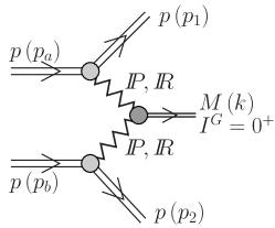
Figure 1: The exchange mechanisms for central exclusive meson production in proton-proton collisions.

We shall be mainly interested in the $I\!\!PI\!\!P$-fusion giving the meson $M$. It is clear from Fig. 1 that in order to calculate this contribution we must know the $I\!\!Ppp$ vertex, the effective $I\!\!P$ propagator and the $I\!\!PI\!\!PM$ vertex. This propagator and these vertices will now be discussed, both, for the tensorial and vectorial ansatz for the pomeron $I\!\!P$.

II.2 Scalar and pseudoscalar meson production

In this section we study central production of scalar and pseudoscalar mesons, that is, the reaction (1) with $J^{PC}=0^{++}$ and $0^{-+}$ mesons $M$. We shall consider pomeron-pomeron fusion, see Fig. 1, for both, the tensorial- and the vectorial-pomeron approaches. In Table 7 of Appendix A we list mesons $M$ in which we are interested. There we also give the values of the lowest orbital angular momentum $l$ and of the corresponding total spin $S$ which can lead to the production of $M$ in the fictitious fusion of two tensorial and vectorial “pomeron particles”. The lower the values of $l$ is, the lower is the angular momentum barrier in the reaction.

We discuss first the tensor-pomeron case. For scalar mesons, $J^{PC}=0^{++}$, the effective Lagrangians and the vertices for $I\!\!PI\!\!P\to M$ are discussed in Appendix A. For the tensorial pomeron the vertex corresponding to the lowest values of $(l,S)$, that is $(l,S)=(0,0)$ plus $(2,2)$, is given in (50). For pseudoscalar mesons, $J^{PC}=0^{-+}$, the tensorial pomeron-pomeron-meson $(I\!\!PI\!\!P\tilde{M})$ coupling corresponding to $(l,S)=(1,1)$, see Table 6 of Appendix A, has the form

$${\cal L}_{I\!\!PI\!\!P\tilde{M}}^{\prime}(x)=-\dfrac{2}{M_{0}}\,g_{I\!\!PI\!\!P\tilde{M}}^{\prime}\,\left[\partial_{\rho}I\!\!P_{\mu\nu}(x)\right]\,\left[\partial_{\sigma}I\!\!P_{\kappa\lambda}(x)\right]\,g^{\mu\kappa}\,\varepsilon^{\nu\lambda\rho\sigma}\,\tilde{\chi}(x)\,.$$ (3)

Here $\tilde{\chi}(x)$ and $I\!\!P_{\mu\nu}(x)$ are the pseudoscalar meson and effective tensor-pomeron field operators, respectively; $M_{0}\equiv 1$ GeV, and $g_{I\!\!PI\!\!P\tilde{M}}^{\prime}$ is a dimensionless coupling constant.

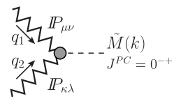
(a) (b)

Figure 2: A sketch of the pomeron-pomeron-pseudoscalar meson vertex for the tensorial (a) and vectorial (b) pomeron fusion.

The $I\!\!PI\!\!P\tilde{M}$ vertex corresponding to $(l,S)=(1,1)$ obtained from (3), see Fig. 2 (a), including a form factor, reads as follows:

$$i\Gamma_{\mu\nu,\kappa\lambda}^{\prime(I\!\!PI\!\!P\to\tilde{M})}(q_{1},q_{2}) = i\,\frac{g_{I\!\!PI\!\!P\tilde{M}}^{\prime}}{2M_{0}}\,\left(g_{\mu\kappa}\varepsilon_{\nu\lambda\rho\sigma}+g_{\nu\kappa}\varepsilon_{\mu\lambda\rho\sigma}+g_{\mu\lambda}\varepsilon_{\nu\kappa\rho\sigma}+g_{\nu\lambda}\varepsilon_{\mu\kappa\rho\sigma}\right)(q_{1}-q_{2})^{\rho}k^{\sigma}$$ (4)

$$\times F_{I\!\!PI\!\!P\tilde{M}}(q_{1}^{2},q_{2}^{2})\,,$$

where the meson four-momentum $k=q_{1}+q_{2}$. Another form for the $I\!\!PI\!\!P\tilde{M}$ coupling corresponding to $(l,S)=(3,3)$ is

$${\cal L}_{I\!\!PI\!\!P\tilde{M}}^{\prime\prime}(x) = -\dfrac{g_{I\!\!PI\!\!P\tilde{M}}^{\prime\prime}}{M_{0}^{3}}\,\varepsilon^{\mu_{1}\mu_{2}\nu_{1}\nu_{2}}\,(\partial_{\mu_{1}}\tilde{\chi}(x))$$ (5)

$$\times[\left(\partial_{\mu_{3}}I\!\!P_{\mu_{4}\nu_{1}}(x)-\partial_{\mu_{4}}I\!\!P_{\mu_{3}\nu_{1}}(x)\right)\stackrel{{\scriptstyle\leftrightarrow}}{{\partial_{\mu_{2}}}}\left(\partial^{\mu_{3}}I\!\!P^{\mu_{4}}_{\quad\nu_{2}}(x)-\partial^{\mu_{4}}I\!\!P^{\mu_{3}}_{\quad\nu_{2}}(x)\right)]\,,$$

where the asymmetric derivative has the form $\stackrel{{\scriptstyle\leftrightarrow}}{{\partial_{\mu}}}=\stackrel{{\scriptstyle\rightarrow}}{{\partial_{\mu}}}-\stackrel{{\scriptstyle\leftarrow}}{{\partial_{\mu}}}$. From (5) we get the vertex, including a form factor, as follows

$$i\Gamma_{\mu\nu,\kappa\lambda}^{\prime\prime(I\!\!PI\!\!P\to\tilde{M})}(q_{1},q_{2}) = i\,\frac{g_{I\!\!PI\!\!P\tilde{M}}^{\prime\prime}}{M_{0}^{3}}\,\{\varepsilon_{\nu\lambda\rho\sigma}\left[q_{1\kappa}q_{2\mu}-(q_{1}q_{2})g_{\mu\kappa}\right]+\varepsilon_{\mu\lambda\rho\sigma}\left[q_{1\kappa}q_{2\nu}-(q_{1}q_{2})g_{\nu\kappa}\right]$$ (6)

$$+\,\varepsilon_{\nu\kappa\rho\sigma}\left[q_{1\lambda}q_{2\mu}-(q_{1}q_{2})g_{\mu\lambda}\right]+\varepsilon_{\mu\kappa\rho\sigma}\left[q_{1\lambda}q_{2\nu}-(q_{1}q_{2})g_{\nu\lambda}\right]\}(q_{1}-q_{2})^{\rho}k^{\sigma}$$

$$\times F_{I\!\!PI\!\!P\tilde{M}}(q_{1}^{2},q_{2}^{2})\,$$

with $g_{I\!\!PI\!\!P\tilde{M}}^{\prime\prime}$ a dimensionless coupling constant. As complete vertex we take the sum of (4) and (6)

$$i\Gamma_{\mu\nu,\kappa\lambda}^{(I\!\!PI\!\!P\to\tilde{M})}(q_{1},q_{2})=i\Gamma_{\mu\nu,\kappa\lambda}^{\prime(I\!\!PI\!\!P\to\tilde{M})}(q_{1},q_{2})+i\Gamma_{\mu\nu,\kappa\lambda}^{\prime\prime(I\!\!PI\!\!P\to\tilde{M})}(q_{1},q_{2})\,.$$ (7)

It can be checked that this vertex satisfies the identities

$$\Gamma_{\mu\nu,\kappa\lambda}^{(I\!\!PI\!\!P\to\tilde{M})}(q_{1},q_{2})=\Gamma_{\kappa\lambda,\mu\nu}^{(I\!\!PI\!\!P\to\tilde{M})}(q_{2},q_{1})\,,$$

$$g^{\mu\nu}\Gamma_{\mu\nu,\kappa\lambda}^{(I\!\!PI\!\!P\to\tilde{M})}(q_{1},q_{2})=0\,,\quad g^{\kappa\lambda}\Gamma_{\mu\nu,\kappa\lambda}^{(I\!\!PI\!\!P\to\tilde{M})}(q_{1},q_{2})=0\,.$$ (8)

Now we can write down the $I\!\!PI\!\!P$-fusion contributions to the Born amplitudes for the scalar and pseudoscalar meson exclusive production. We find for a $0^{++}$ meson $M$

$$\Braket{p(p_{1},\lambda_{1}),p(p_{2},\lambda_{2}),M(k)}{{\cal T}}{p(p_{a},\lambda_{a}),p(p_{b},\lambda_{b})}\mid_{I\!\!PI\!\!P}\;\equiv$$

$${\cal M}^{2\to 3}_{\lambda_{a}\lambda_{b}\to\lambda_{1}\lambda_{2}M}\mid_{I\!\!PI\!\!P}\;=(-i)\bar{u}(p_{1},\lambda_{1})i\Gamma_{\mu_{1}\nu_{1}}^{(I\!\!Ppp)}(p_{1},p_{a})u(p_{a},\lambda_{a})$$

$$\qquad\qquad\qquad\qquad\quad\times i\Delta^{(I\!\!P)\,\mu_{1}\nu_{1},\kappa_{1}\lambda_{1}}(s_{13},t_{1})\;\;i\Gamma_{\kappa_{1}\lambda_{1},\kappa_{2}\lambda_{2}}^{(I\!\!PI\!\!P\to M)}(q_{1},q_{2})\;\;i\Delta^{(I\!\!P)\,\kappa_{2}\lambda_{2},\mu_{2}\nu_{2}}(s_{23},t_{2})$$

$$\qquad\qquad\qquad\qquad\quad\times\bar{u}(p_{2},\lambda_{2})i\Gamma_{\mu_{2}\nu_{2}}^{(I\!\!Ppp)}(p_{2},p_{b})u(p_{b},\lambda_{b})\,.$$ (9)

Here $\Delta^{(I\!\!P)}$ and $\Gamma^{(I\!\!Ppp)}$ denote the effective propagator and proton vertex function, respectively, for the tensorial pomeron. For the explicit expressions, see Appendix A, (30) to (34) and for the $I\!\!PI\!\!PM$ vertex (50). For a pseudoscalar meson $\tilde{M}$ the amplitude is similar with $\Gamma_{\kappa_{1}\lambda_{1},\kappa_{2}\lambda_{2}}^{(I\!\!PI\!\!P\to M)}$ replaced by $\Gamma_{\kappa_{1}\lambda_{1},\kappa_{2}\lambda_{2}}^{(I\!\!PI\!\!P\to\tilde{M})}$ in (9).

Explicitly we obtain from (9), using the expressions from Appendix A, the amplitude for exclusive production of a scalar meson $M$ as

$${\cal M}^{2\to 3}_{\lambda_{a}\lambda_{b}\to\lambda_{1}\lambda_{2}M}\mid_{I\!\!PI\!\!P}\;=-\left(3\beta_{I\!\!PNN}\right)^{2}\,F_{1}(t_{1})\,F_{1}(t_{2})\,F_{I\!\!PI\!\!PM}(t_{1},t_{2})$$

$$\times\bar{u}(p_{1},\lambda_{1})\gamma^{\mu_{1}}(p_{1}+p_{a})^{\nu_{1}}u(p_{a},\lambda_{a})\;\frac{1}{2s_{13}}\left(-is_{13}\alpha^{\prime}_{I\!\!P}\right)^{\alpha_{I\!\!P}(t_{1})-1}$$

$$\times\left.\Bigl{[}g_{I\!\!PI\!\!PM}^{\prime}M_{0}\Bigl{(}g_{\mu_{1}\mu_{2}}g_{\nu_{1}\nu_{2}}+g_{\mu_{1}\nu_{2}}g_{\nu_{1}\mu_{2}}-\frac{1}{2}g_{\mu_{1}\nu_{1}}g_{\mu_{2}\nu_{2}}\Bigr{)}+\frac{g_{I\!\!PI\!\!PM}^{\prime\prime}}{2M_{0}}\right.$$

$$\left.\times\Bigr{(}q_{1\mu_{2}}q_{2\mu_{1}}g_{\nu_{1}\nu_{2}}+q_{1\mu_{2}}q_{2\nu_{1}}g_{\mu_{1}\nu_{2}}+q_{1\nu_{2}}q_{2\mu_{1}}g_{\nu_{1}\mu_{2}}+q_{1\nu_{2}}q_{2\nu_{1}}g_{\mu_{1}\mu_{2}}-2(q_{1}q_{2})(g_{\mu_{1}\mu_{2}}g_{\nu_{1}\nu_{2}}+g_{\nu_{1}\mu_{2}}g_{\mu_{1}\nu_{2}})\Bigr{)}\right.\Bigr{]}$$

$$\times\frac{1}{2s_{23}}\left(-is_{23}\alpha^{\prime}_{I\!\!P}\right)^{\alpha_{I\!\!P}(t_{2})-1}\;\bar{u}(p_{2},\lambda_{2})\gamma^{\mu_{2}}(p_{2}+p_{b})^{\nu_{2}}u(p_{b},\lambda_{b})\,.$$ (10)

The coupling constants $\beta_{I\!\!PNN}$, $g_{I\!\!PI\!\!PM}^{\prime}$, and $g_{I\!\!PI\!\!PM}^{\prime\prime}$ are defined in (30), (46), and (48), and the form factors $F_{1}$ and $F_{I\!\!PI\!\!PM}$ in (31) and (51), respectively. Similarly, we obtain the amplitude for production of a pseudoscalar meson $\tilde{M}$ as

$${\cal M}^{2\to 3}_{\lambda_{a}\lambda_{b}\to\lambda_{1}\lambda_{2}\tilde{M}}\mid_{I\!\!PI\!\!P}\;=-(3\beta_{I\!\!PNN})^{2}\,F_{1}(t_{1})\,F_{1}(t_{2})\,F_{I\!\!PI\!\!P\tilde{M}}(t_{1},t_{2})$$

$$\times\bar{u}(p_{1},\lambda_{1})\gamma^{\mu_{1}}(p_{1}+p_{a})^{\nu_{1}}u(p_{a},\lambda_{a})\;\frac{1}{2s_{13}}\left(-is_{13}\alpha^{\prime}_{I\!\!P}\right)^{\alpha_{I\!\!P}(t_{1})-1}$$

$$\times\left.\Bigl{[}\Bigl{(}\frac{g_{I\!\!PI\!\!P\tilde{M}}}{2M_{0}}-\frac{g_{I\!\!PI\!\!P\tilde{M}}^{\prime\prime}}{M_{0}^{3}}(q_{1}q_{2})\Bigr{)}\Bigl{(}g_{\mu_{1}\mu_{2}}\varepsilon_{\nu_{1}\nu_{2}\rho\sigma}+g_{\nu_{1}\mu_{2}}\varepsilon_{\mu_{1}\nu_{2}\rho\sigma}+g_{\mu_{1}\nu_{2}}\varepsilon_{\nu_{1}\mu_{2}\rho\sigma}+g_{\nu_{1}\nu_{2}}\varepsilon_{\mu_{1}\mu_{2}\rho\sigma}\Bigr{)}\right.$$

$$\left.+\frac{g_{I\!\!PI\!\!P\tilde{M}}^{\prime\prime}}{M_{0}^{3}}\Bigl{(}\varepsilon_{\nu_{1}\nu_{2}\rho\sigma}q_{1\mu_{2}}q_{2\mu_{1}}+\varepsilon_{\mu_{1}\nu_{2}\rho\sigma}q_{1\mu_{2}}q_{2\nu_{1}}+\varepsilon_{\nu_{1}\mu_{2}\rho\sigma}q_{1\nu_{2}}q_{2\mu_{1}}+\varepsilon_{\mu_{1}\mu_{2}\rho\sigma}q_{1\nu_{2}}q_{2\nu_{1}}\Bigr{)}\right.\Bigr{]}(q_{1}-q_{2})^{\rho}k^{\sigma}$$

$$\times\frac{1}{2s_{23}}\left(-is_{23}\alpha^{\prime}_{I\!\!P}\right)^{\alpha_{I\!\!P}(t_{2})-1}\;\bar{u}(p_{2},\lambda_{2})\gamma^{\mu_{2}}(p_{2}+p_{b})^{\nu_{2}}u(p_{b},\lambda_{b})\,;$$ (11)

see (4), (6), (30), (31), and (51).

The same steps can now be repeated in the model of the vector pomeron. The Born amplitude for the production of a $0^{++}$ meson $M$ via $I\!\!P_{V}I\!\!P_{V}$-fusion can be written as

$${\cal M}^{2\to 3}_{\lambda_{a}\lambda_{b}\to\lambda_{1}\lambda_{2}M}\mid_{I\!\!P_{V}I\!\!P_{V}} = (-i)\bar{u}(p_{1},\lambda_{1})i\Gamma_{\mu_{1}}^{(I\!\!P_{V}pp)}(p_{1},p_{a})u(p_{a},\lambda_{a})$$ (12)

$$\times i\Delta^{(I\!\!P_{V})\,\mu_{1}\nu_{1}}(s_{13},t_{1})\;\;i\Gamma_{\nu_{1}\nu_{2}}^{(I\!\!P_{V}I\!\!P_{V}\to M)}(q_{1},q_{2})\;\;i\Delta^{(I\!\!P_{V})\,\nu_{2}\mu_{2}}(s_{23},t_{2})$$

$$\times\bar{u}(p_{2},\lambda_{2})i\Gamma_{\mu_{2}}^{(I\!\!P_{V}pp)}(p_{2},p_{b})u(p_{b},\lambda_{b})\,.$$

The effective Lagrangian and the vertices for $I\!\!P_{V}I\!\!P_{V}\to M$ are discussed in Appendix B; see (56), (57), and (64). Explicitly we obtain

$${\cal M}^{2\to 3}_{\lambda_{a}\lambda_{b}\to\lambda_{1}\lambda_{2}M}\mid_{I\!\!P_{V}I\!\!P_{V}} = -(3\beta_{I\!\!PNN})^{2}\,F_{1}(t_{1})\,F_{1}(t_{2})\,F_{I\!\!PI\!\!PM}(t_{1},t_{2})$$ (13)

$$\times\bar{u}(p_{1},\lambda_{1})\gamma^{\mu_{1}}u(p_{a},\lambda_{a})\,g_{\mu_{1}\nu_{1}}\,\left(-is_{13}\alpha^{\prime}_{I\!\!P}\right)^{\alpha_{I\!\!P}(t_{1})-1}\,$$

$$\times\Bigl{[}\frac{2}{M_{0}}\,g_{I\!\!P_{V}I\!\!P_{V}M}^{\prime}\,g^{\nu_{1}\nu_{2}}\,+\frac{2}{M_{0}^{3}}\,g_{I\!\!P_{V}I\!\!P_{V}M}^{\prime\prime}\,\Bigl{(}q_{2}^{\nu_{1}}q_{1}^{\nu_{2}}-(q_{1}q_{2})g^{\nu_{1}\nu_{2}}\Bigr{)}\Bigr{]}$$

$$\times g_{\nu_{2}\mu_{2}}\,\left(-is_{23}\alpha^{\prime}_{I\!\!P}\right)^{\alpha_{I\!\!P}(t_{2})-1}\,\bar{u}(p_{2},\lambda_{2})\gamma^{\mu_{2}}u(p_{b},\lambda_{b})\,.$$

Now we turn to the production of a pseudoscalar meson $\tilde{M}$ via $I\!\!P_{V}I\!\!P_{V}$-fusion. The first step is to construct an effective coupling Lagrangian $I\!\!P_{V}I\!\!P_{V}\tilde{M}$. Traditionally this is done in analogy to the $\gamma\gamma\pi^{0}$ coupling which is given by the Adler-Bell-Jackiw anomaly (for a review see chapter 22 of Weinberg ). In this way we get

$${\cal L}_{I\!\!P_{V}I\!\!P_{V}\tilde{M}}^{\prime}(x)=\frac{g_{I\!\!P_{V}I\!\!P_{V}\tilde{M}}^{\prime}}{16M_{0}}\,\left[\partial_{\mu}I\!\!P_{V\nu}(x)-\partial_{\nu}I\!\!P_{V\mu}(x)\right]\,\left[\partial_{\rho}I\!\!P_{V\sigma}(x)-\partial_{\sigma}I\!\!P_{V\rho}(x)\right]\,\varepsilon^{\mu\nu\rho\sigma}\,\tilde{\chi}(x)$$

(14)

with $g_{I\!\!P_{V}I\!\!P_{V}\tilde{M}}^{\prime}$ a dimensionless coupling constant.

The corresponding vertex, including a form factor, reads as follows (see Fig. 2 (b)):

$$i\Gamma_{\mu\nu}^{\prime(I\!\!P_{V}I\!\!P_{V}\to\tilde{M})}(q_{1},q_{2})=i\,\frac{g_{I\!\!P_{V}I\!\!P_{V}\tilde{M}}^{\prime}}{2M_{0}}\,\varepsilon_{\mu\nu\rho\sigma}q_{1}^{\rho}q_{2}^{\sigma}\,F_{I\!\!PI\!\!P\tilde{M}}(q_{1}^{2},q_{2}^{2})\,.$$ (15)

It is easy to see that in the fictitious reaction (59) the coupling (14), (15) gives $(l,S)=(1,1)$. Note that in our framework we have for $I\!\!P_{T}I\!\!P_{T}$-fusion two values, $(l,S)=(1,1)$ and $(3,3)$, which can lead to a pseudoscalar meson; see Table 6 in Appendix A. Correspondingly, we have two independent couplings, (3) and (5). For $I\!\!P_{V}I\!\!P_{V}$-fusion, on the other hand, we find from Table 8 in Appendix B that only $(l,S)=(1,1)$ can lead to a pseudoscalar meson, thus, only the coupling (14) is possible there. This clear difference between the $I\!\!P_{T}$ and $I\!\!P_{V}$ ansätze can be exploited for experimentally distinguishing the two cases.

The amplitude for the production of a $J^{PC}=0^{-+}$ meson $\tilde{M}$ via $I\!\!P_{V}I\!\!P_{V}$-fusion can now be written down as in (12) with the $I\!\!P_{V}I\!\!P_{V}\tilde{M}$ vertex from (15). Explicitly this gives

$${\cal M}^{2\to 3}_{\lambda_{a}\lambda_{b}\to\lambda_{1}\lambda_{2}\tilde{M}}\mid_{I\!\!P_{V}I\!\!P_{V}}\,=\, -(3\beta_{I\!\!PNN})^{2}\,F_{1}(t_{1})\,F_{1}(t_{2})\,F_{I\!\!PI\!\!P\tilde{M}}(t_{1},t_{2})\,\frac{g_{I\!\!P_{V}I\!\!P_{V}\tilde{M}}^{\prime}}{2M_{0}^{3}}$$ (16)

$$\times\bar{u}(p_{1},\lambda_{1})\gamma^{\mu_{1}}u(p_{a},\lambda_{a})\,g_{\mu_{1}\nu_{1}}\,\left(-is_{13}\alpha^{\prime}_{I\!\!P}\right)^{\alpha_{I\!\!P}(t_{1})-1}$$

$$\times\epsilon^{\nu_{1}\nu_{2}\rho\sigma}\,q_{1\rho}q_{2\sigma}$$

$$\times g_{\nu_{2}\mu_{2}}\,\left(-is_{23}\alpha^{\prime}_{I\!\!P}\right)^{\alpha_{I\!\!P}(t_{2})-1}\,\bar{u}(p_{2},\lambda_{2})\gamma^{\mu_{2}}u(p_{b},\lambda_{b})\,.$$

In KMV99 also (vector pomeron)-(vector pomeron) fusion was considered as the dominant mechanism of the $\eta^{\prime}$-meson production. In order to estimate this contribution, the Donnachie-Landshoff energy dependence of the pomeron exchange DL was used.

We shall now consider the high-energy small-angle limit, see Appendix D, for both the tensorial and vectorial pomeron fusion reactions giving the mesons $M$ and $\tilde{M}$. With (110) to (124) we get from (10) and (11) for the tensorial pomeron

$${\cal M}^{2\to 3}_{\lambda_{a}\lambda_{b}\to\lambda_{1}\lambda_{2}M}\mid_{I\!\!PI\!\!P} \cong -2s\,(3\beta_{I\!\!PNN})^{2}\,F_{1}(t_{1})\,F_{1}(t_{2})\,F_{I\!\!PI\!\!PM}(t_{1},t_{2})$$ (17)

$$\times\frac{M_{0}}{m_{M}^{2}}\Bigl{(}g_{I\!\!PI\!\!PM}^{\prime}+g_{I\!\!PI\!\!PM}^{\prime\prime}\,\frac{1}{M_{0}^{2}}\,\vec{p}_{1\perp}\cdot\vec{p}_{2\perp}\Bigr{)}$$

$$\times\left(-is_{13}\alpha^{\prime}_{I\!\!P}\right)^{\alpha_{I\!\!P}(t_{1})-1}\;\left(-is_{23}\alpha^{\prime}_{I\!\!P}\right)^{\alpha_{I\!\!P}(t_{2})-1}$$

$$\times\delta_{\lambda_{1}\lambda_{a}}\delta_{\lambda_{2}\lambda_{b}}\,,$$

$${\cal M}^{2\to 3}_{\lambda_{a}\lambda_{b}\to\lambda_{1}\lambda_{2}\tilde{M}}\mid_{I\!\!PI\!\!P} \cong -(3\beta_{I\!\!PNN})^{2}\,F_{1}(t_{1})\,F_{1}(t_{2})\,F_{I\!\!PI\!\!P\tilde{M}}(t_{1},t_{2})$$ (18)

$$\times\frac{1}{m_{\tilde{M}}^{2}}\Bigl{[}\frac{g_{I\!\!PI\!\!P\tilde{M}}^{\prime}}{M_{0}}+\frac{g_{I\!\!PI\!\!P\tilde{M}}^{\prime\prime}}{sM_{0}^{3}}\,\Bigl{(}(q_{1},p_{2}+p_{b})(q_{2},p_{1}+p_{a})-(q_{1},q_{2})(p_{1}+p_{a},p_{2}+p_{b})\Bigr{)}\Bigr{]}$$

$$\times\varepsilon_{\mu\nu\rho\sigma}(p_{1}+p_{a})^{\mu}(p_{2}+p_{b})^{\nu}(q_{1}-q_{2})^{\rho}k^{\sigma}$$

$$\times\left(-is_{13}\alpha^{\prime}_{I\!\!P}\right)^{\alpha_{I\!\!P}(t_{1})-1}\;\left(-is_{23}\alpha^{\prime}_{I\!\!P}\right)^{\alpha_{I\!\!P}(t_{2})-1}$$

$$\times\delta_{\lambda_{1}\lambda_{a}}\delta_{\lambda_{2}\lambda_{b}}$$

$$\cong -4s\,(3\beta_{I\!\!PNN})^{2}\,F_{1}(t_{1})\,F_{1}(t_{2})\,F_{I\!\!PI\!\!P\tilde{M}}(t_{1},t_{2})$$

$$\times\frac{1}{m_{\tilde{M}}^{2}M_{0}}|\vec{p}_{1\perp}||\vec{p}_{2\perp}|\sin\phi_{pp}\Bigl{(}g_{I\!\!PI\!\!P\tilde{M}}^{\prime}+g_{I\!\!PI\!\!P\tilde{M}}^{\prime\prime}\,\frac{2}{M_{0}^{2}}|\vec{p}_{1\perp}||\vec{p}_{2\perp}|\cos\phi_{pp}\Bigr{)}$$

$$\times\left(-is_{13}\alpha^{\prime}_{I\!\!P}\right)^{\alpha_{I\!\!P}(t_{1})-1}\;\left(-is_{23}\alpha^{\prime}_{I\!\!P}\right)^{\alpha_{I\!\!P}(t_{2})-1}$$

$$\times\delta_{\lambda_{1}\lambda_{a}}\delta_{\lambda_{2}\lambda_{b}}\,.$$

For the vectorial pomeron we get in this limit from (13) and (16) the expressions (17) and (18), respectively, but with the replacements:

$$g_{I\!\!PI\!\!PM}^{\prime}\to\frac{2m_{M}^{2}}{M_{0}^{2}}\,g_{I\!\!P_{V}I\!\!P_{V}M}^{\prime}\,,\quad g_{I\!\!PI\!\!PM}^{\prime\prime}\to\frac{2m_{M}^{2}}{M_{0}^{2}}\,g_{I\!\!P_{V}I\!\!P_{V}M}^{\prime\prime}\,,$$ (19)

$$g_{I\!\!PI\!\!P\tilde{M}}^{\prime}\to\frac{m_{\tilde{M}}^{2}}{4M_{0}^{2}}\,g_{I\!\!P_{V}I\!\!P_{V}\tilde{M}}^{\prime}\,,\quad g_{I\!\!PI\!\!P\tilde{M}}^{\prime\prime}\to 0\,.$$ (20)

We see that for the vectorial pomeron the term $\propto\cos\phi_{pp}\sin\phi_{pp}$ in (18) is absent.

Going now from high to intermediate collision energies we must expect besides pomeron-pomeron fusion also reggeon-pomeron (pomeron-reggeon) and reggeon-reggeon fusion to become important; see Fig. 1. The relevant scales for these non-leading terms should be given by the subenergies squared $s_{13}$ and $s_{23}$ in (2). We have to consider for the first non-leading contributions those from the Regge trajectories with intercept $\alpha_{I\!\!R}(0)\approx 0.5$, that is, the $f_{2}$, $a_{2}$, $\omega$ and $\rho$ trajectories which we shall denote by $f_{2I\!\!R}$, $a_{2I\!\!R}$, $\omega_{I\!\!R}$ and $\rho_{I\!\!R}$, respectively. In Ref. EMN13 effective propagators for these reggeons and reggeon-proton-proton vertices are given. The $C=+1$ reggeons $f_{2I\!\!R}$ and $a_{2I\!\!R}$ are treated as effective tensor exchanges, the $C=-1$ reggeons $\omega_{I\!\!R}$ and $\rho_{I\!\!R}$ as effective vector exchanges. We shall make use of the results of EMN13 in the following.

To give an example we discuss the contribution of $\omega_{I\!\!R}\omega_{I\!\!R}$-fusion to the production of a pseudoscalar meson $\tilde{M}$; see Fig. 1 with $I\!\!R=\omega_{I\!\!R}$ and $M\to\tilde{M}$. The effective $\omega_{I\!\!R}$ propagator and the $\omega_{I\!\!R}pp$ vertex are given in EMN13 as follows:

• $\omega_{I\!\!R}$ propagator

  $$i\Delta_{\mu\nu}^{(\omega_{I\!\!R})}(s,t)=i\,g_{\mu\nu}\,\frac{1}{M_{-}^{2}}\,\left(-is\alpha^{\prime}_{I\!\!R}\right)^{\alpha_{I\!\!R}(t)-1}$$ (21)

  with the parameters (see DDLN ) of the Regge trajectory

  $$\alpha_{I\!\!R}(t)=\alpha_{I\!\!R}(0)+\alpha^{\prime}_{I\!\!R}\,t\,,$$

  $$\alpha_{I\!\!R}(0)=0.5475,\quad\alpha^{\prime}_{I\!\!R}=0.9\;\mathrm{GeV}^{-2}\,,$$ (22)

  and the mass scale $M_{-}=1.41$ GeV.

• $\omega_{I\!\!R}pp$ vertex

  $$i\Gamma_{\mu}^{(\omega_{I\!\!R}pp)}(p^{\prime},p)=-i\,g_{\omega_{I\!\!R}pp}\,F_{1}\bigl{(}(p^{\prime}-p)^{2}\bigr{)}\,\gamma_{\mu}\,,$$ (23)

  where $g_{\omega_{I\!\!R}pp}=8.65$.

For the $\omega_{I\!\!R}\omega_{I\!\!R}\tilde{M}$ vertex we shall make an ansatz in complete analogy to (14), (15) for the vectorial pomeron. We get then

$$i\Gamma_{\mu\nu}^{(\omega_{I\!\!R}\omega_{I\!\!R}\to\tilde{M})}(q_{1},q_{2})=i\,\frac{g_{\omega_{I\!\!R}\omega_{I\!\!R}\tilde{M}}}{2M_{0}}\,\varepsilon_{\mu\nu\rho\sigma}q_{1}^{\rho}q_{2}^{\sigma}\,F_{\omega_{I\!\!R}\omega_{I\!\!R}\tilde{M}}(q_{1}^{2},q_{2}^{2})\,,$$ (24)

where $g_{\omega_{I\!\!R}\omega_{I\!\!R}\tilde{M}}$ is a dimensionless coupling constant.

Using (21) to (24) the Born amplitude for the $\omega_{I\!\!R}\omega_{I\!\!R}$-fusion giving a pseudoscalar meson $\tilde{M}$ can be parametrized as

$${\cal M}^{2\to 3}_{\lambda_{a}\lambda_{b}\to\lambda_{1}\lambda_{2}\tilde{M}}\mid_{\omega_{I\!\!R}\omega_{I\!\!R}}=\; (g_{\omega_{I\!\!R}pp})^{2}\,F_{1}(t_{1})\,F_{1}(t_{2})\,F_{\omega_{I\!\!R}\omega_{I\!\!R}\tilde{M}}(t_{1},t_{2})\,\frac{g_{\omega_{I\!\!R}\omega_{I\!\!R}\tilde{M}}}{2M_{0}}$$ (25)

$$\times\bar{u}(p_{1},\lambda_{1})\gamma^{\mu_{1}}u(p_{a},\lambda_{a})$$

$$\times g_{\mu_{1}\nu_{1}}\,(M_{-})^{-2}\,\left(-is_{13}\alpha^{\prime}_{I\!\!R}\right)^{\alpha_{I\!\!R}(t_{1})-1}$$

$$\times\epsilon^{\nu_{1}\nu_{2}\rho\sigma}\,q_{1\rho}q_{2\sigma}$$

$$\times g_{\nu_{2}\mu_{2}}\,(M_{-})^{-2}\,\left(-is_{23}\alpha^{\prime}_{I\!\!R}\right)^{\alpha_{I\!\!R}(t_{2})-1}$$

$$\times\bar{u}(p_{2},\lambda_{2})\gamma^{\mu_{2}}u(p_{b},\lambda_{b})\,.$$

At even lower energies, for $s_{13}$ and $s_{23}$ near the threshold value $s_{thr}=(m_{p}+m_{\tilde{M}})^{2}$, respectively $s_{thr}=(m_{p}+m_{M})^{2}$ for a $0^{++}$ meson $M$, the exchange of reggeons in Fig. 1 should be replaced by particle exchanges. As an example we give the amplitudes for $\eta$ and $\eta^{\prime}$ production at low energies $\sqrt{s_{13}}$ and $\sqrt{s_{23}}$. It is known from the low energy phenomenology that both $\rho\rho$ and $\omega\omega$ mesons couple to $\eta$ and $\eta^{\prime}$ mesons. The $\omega\omega\tilde{M}$ vertex required for constructing the meson-exchange current is derived from the Lagrangian densities

$${\cal L}_{\omega\omega\tilde{M}}(x)=\frac{g_{\omega\omega\tilde{M}}}{2m_{\omega}}\,\left[\partial_{\mu}\omega_{\nu}(x)\right]\left[\partial_{\rho}\omega_{\sigma}(x)\right]\,\varepsilon^{\mu\nu\rho\sigma}\,\tilde{\chi}(x)\,$$ (26)

and reads

$$i\Gamma_{\mu\nu}^{(\omega\omega\to\tilde{M})}(q_{1},q_{2})=i\,\frac{g_{\omega\omega\tilde{M}}}{m_{\omega}}\,\varepsilon_{\mu\nu\rho\sigma}q_{1}^{\rho}q_{2}^{\sigma}\,F_{\omega\omega\tilde{M}}(q_{1}^{2},q_{2}^{2})\,.$$ (27)

The Born amplitude for the $\omega\omega$-fusion giving $\tilde{M}=\eta^{\prime}$ or $\eta$ can be written as

$${\cal M}^{2\to 3}_{\lambda_{a}\lambda_{b}\to\lambda_{1}\lambda_{2}\tilde{M}}\mid_{\omega\omega}=\; (g_{\omega pp})^{2}\,F_{\omega}(t_{1})\,F_{\omega}(t_{2})\,F_{\omega\omega\tilde{M}}(t_{1},t_{2})\,\frac{g_{\omega\omega\tilde{M}}}{m_{\omega}}$$ (28)

$$\times\bar{u}(p_{1},\lambda_{1})\gamma^{\mu_{1}}u(p_{a},\lambda_{a})$$

$$\times\frac{-g_{\mu_{1}\nu_{1}}+q_{1\mu_{1}}q_{1\nu_{1}}/m_{\omega}^{2}}{t_{1}-m_{\omega}^{2}}\,\epsilon^{\nu_{1}\nu_{2}\rho\sigma}\,q_{1\rho}q_{2\sigma}\,\frac{-g_{\nu_{2}\mu_{2}}+q_{2\nu_{2}}q_{2\mu_{2}}/m_{\omega}^{2}}{t_{2}-m_{\omega}^{2}}$$

$$\times\bar{u}(p_{2},\lambda_{2})\gamma^{\mu_{2}}u(p_{b},\lambda_{b})\,.$$

The coupling constants $g_{\omega\omega\eta^{\prime}}=4.9$ NH04 ; KK08 , $g_{\omega\omega\eta}=4.84$ NSL02 ; NYH11 are known from low energy phenomenology. In the present calculations we take the $\omega pp$ coupling constant $g_{\omega pp}=10$. Here we use form factors $F_{\omega\omega\tilde{M}}(t_{1},t_{2})=F_{\omega}(t_{1})\,F_{\omega}(t_{2})$ for both exponential (55) or monopole (54) approaches. At larger subsystem energies squared, $s_{13},s_{23}\gg s_{thr}$, one should use reggeons rather than mesons. The “reggeization” of the amplitude given in Eq. (28) is included here only approximately by a factor assuring asymptotically correct high energy dependence

$${\cal F}=\left(\frac{s_{13}}{s_{thr}}\right)^{\frac{2}{\pi}\arctan[(s_{13}-s_{thr})/\Lambda_{thr}^{2}](\alpha_{I\!\!R}(t_{1})-1)}\left(\frac{s_{23}}{s_{thr}}\right)^{\frac{2}{\pi}\arctan[(s_{23}-s_{thr})/\Lambda_{thr}^{2}](\alpha_{I\!\!R}(t_{2})-1)}\,,$$ (29)

where $\Lambda_{thr}=1$ GeV and $\alpha_{I\!\!R}(0)=0.5$ and $\alpha^{\prime}_{I\!\!R}=0.9$ GeV^-2.

II.3 Existing experimental data

A big step in the investigation of central meson production process (1) has been taken by the WA91 and WA102 Collaborations, which have reported remarkable kinematical dependences and different effects; see Ref. WA91_PLB388 ; WA102_PLB397 ; WA102_PLB427 ; WA102_PLB462 ; WA102_PLB467 ; WA102_PLB474 ; kirk00 . The WA102 experiment at CERN was the first to discover a strong dependence of the cross section on the azimuthal angle between the momenta transferred to the two protons, a feature that was not expected from standard pomeron phenomenology. This result inspired some phenomenological works Close pointing to a possible analogy between the pomeron and vector particles as had been suggested in DL (see also chapter 3.7 of DDLN ).

Close and his collaborators have even proposed to use transverse momenta correlations of outgoing protons as tool to discriminate different intrinsic structures of the centrally produced object (“glueball filter”); see Close ; CK97 . In particular, the production of scalar mesons such as $f_{0}(980)$, $f_{0}(1500)$, $f_{0}(1710)$ was found to be considerably enhanced at small $dP_{\perp}$, while the production of pseudoscalars such as $\eta$, $\eta^{\prime}$ at large $dP_{\perp}$; see Fig.3 of kirk00 . Here $dP_{\perp}=|d\vec{P}_{\perp}|$ with $d\vec{P}_{\perp}$ the difference of the transverse momenta of the two outgoing protons in (1); see (106). In Ref. WA102_PLB462 ; kirk00 a study was performed of resonance production rates as a function of $dP_{\perp}$. It was observed that all the undisputed $q\bar{q}$ states (i.e. $\eta$, $\eta^{\prime}$, $f_{1}(1285)$ etc.) are suppressed as $dP_{\perp}\to 0$, whereas the glueball candidates, e.g. $f_{0}(1500)$, $f_{2}(1950)$ are prominent. It is also interesting that the $f_{1}(1420)$ state disappears at small $dP_{\perp}$ relative to large $dP_{\perp}$. As can be seen from kirk00 the mesons $\rho^{0}(770)$, $f_{2}(1270)$, and $f_{2}^{\prime}(1525)$ are produced preferentially at large $dP_{\perp}$ and their cross sections peak at $\phi_{pp}=\pi$, i.e. the outgoing protons are on opposite sides of the beam. In contrast, for the ’enigmatic’ $f_{0}(980)$, $f_{0}(1500)$ and $f_{0}(1710)$ states the cross sections peak at $\phi_{pp}=0$. So far, no dynamical explanation of this empirical observation has been suggested, so the challenge for theory is to understand the dynamics behind this “glueball filter”.

In Ref. WA76_ZPC51 the study of the $|t|=|t_{1}+t_{2}|$ dependence of the resonances observed in the $\pi^{+}\pi^{-}$ and $K^{+}K^{-}$ mass spectra at $\sqrt{s}=23.8$ GeV was considered. It has been observed that $\rho(770)$, $\phi(1020)$, $f_{2}(1270)$ and $f^{\prime}_{2}(1525)$ resonances are produced more at the high-$|t|$ region ($|t|>0.3$ GeV²) and at low $|t|$ their signals are suppressed. The suppression of the $\rho$ and $f_{2}(1270)$ signals in the low-$|t|$ region is also present at $\sqrt{s}=12.7$ GeV for the $\pi^{+}p\to\pi^{+}(\pi^{+}\pi^{-})p$ reaction; see WA76_ZPC51 . In addition, the $dP_{\perp}$, $\phi_{pp}$ and $|t|$ distributions observed in the analysis of the $\pi^{+}\pi^{-}$ final state for the $f_{0}(1370)$ and $f_{0}(1500)$ mesons are similar to what was found in the $\pi^{+}\pi^{-}\pi^{+}\pi^{-}$ channel WA102_PLB474 .

Table 1: Experimental results for the ratios of the cross sections for the different mesons at $\sqrt{s}=29.1$ GeV and 12.7 GeV.

	$\eta^{\prime}$	$\rho(770)$	$f_{0}(980)$	$f_{0}(1500)$	$f_{2}(1270)$
$\frac{\sigma(\sqrt{s}=29.1\,GeV)}{\sigma(\sqrt{s}=12.7\,GeV)}$	0.72 $\pm$ 0.16 WA102_PLB467	0.36 $\pm$ 0.05 WA102_PLB462	1.28 $\pm$ 0.21 WA102_PLB462	1.07 $\pm$ 0.14 WA102_PLB462	0.98 $\pm$ 0.13 WA102_PLB462

The ratios of experimental the cross sections for the different mesons at $\sqrt{s}=29.1$ GeV and 12.7 GeV has also been determined, see Table 1. Moreover, the WA76 Collaboration reported that the ratio of the $\rho^{0}(770)$ cross section at 23.8 GeV and 12.7 GeV is $0.44\pm 0.07$; cf. kirk00 . Since the $I=1$ states cannot be produced by pomeron-pomeron fusion, the $\rho$ meson signal decreases at high energy. However, large enhancement of the $\rho$ signal at $\sqrt{s}=29.1$ GeV and strong correlation between the directions of the outgoing protons have been observed WA91_PLB388 ; WA102_PLB397 . Similarly, in the case of the $\omega$ meson production, where some ’non-central’ mechanisms are possible CLSS , the cross section is more than twice larger than for the $f_{0}(1500)$ meson, the lightest scalar glueball candidate kirk00 ; SL .

We turn now to our present calculations of cross sections and distributions for the central production reaction (1) with scalar and pseudoscalar mesons.

III Results

Now we wish to compare results of our calculations with existing experimental data. Theoretical predictions for production of various $J^{PC}$ mesonic states for RHIC, Tevatron and LHC, with parameters fixed from the fit to the WA102 experimental data, can then be easily done.

III.1 Scalar meson production

We start with discussing the WA102 data at $\sqrt{s}=29.1$ GeV where total cross sections are given in Table 1 of Ref. kirk00 . We show these cross sections for the mesons of interest to us in Table 2.

Table 2: Experimental results for total cross sections of various mesons in $pp$ collisions at $\sqrt{s}=29.1$ GeV; from Table 1 of Ref. kirk00 .

	$\eta$	$\eta^{\prime}$	$f_{0}(980)$	$f_{0}(1370)$	$f_{0}(1500)$	$f_{0}(1710)$	$f_{0}(2000)$
$\sigma$($\mu$b)	3.86 $\pm$ 0.37	1.72 $\pm$ 0.18	5.71 $\pm$ 0.45	1.75 $\pm$ 0.58	2.91 $\pm$ 0.30	0.25 $\pm$ 0.07	3.14 $\pm$ 0.48

We assume that here the energy is high enough such that we have to consider only pomeron-pomeron-meson ($I\!\!PI\!\!PM$) fusion. We have then determined the corresponding $I\!\!PI\!\!PM$ coupling constants by approximately fitting the results of our calculations to the total cross sections given in Table 2 and the shapes of experimental differential distributions (specific details will be given when discussing differential distributions below). The results depend also on the pomeron-pomeron-meson form factors (51), as discussed in Appendix A, which are not well known, in particular for larger values of $t$. In Table 3 we show our results for these $I\!\!PI\!\!PM$ coupling constants for the tensorial and vectorial pomeron ansätze. The figures in bold face represent our “best” fit. We show the resulting total cross sections, from the coupling $g_{I\!\!PI\!\!PM}^{\prime}$ alone, from $g_{I\!\!PI\!\!PM}^{\prime\prime}$ alone, and from the total which includes, of course, the interference term between the two couplings. The column “no cuts, total” has to be compared to the experimental results shown in Table 2. For the cross section with the cuts in $t_{1}t_{2}$ only normalised differential distributions are available; see below. Thus, our results for the corresponding cross sections there are predictions to be checked in future experiments.

Table 3: The values of the pomeron-pomeron-meson coupling constants of the two models of the pomeron exchanges which are approximately fitted to reproduce the experimental total cross sections from Table 2 and shapes of differential distributions of the WA102 data as discussed below. The resulting cross sections (in $\mu$b) for scalar meson central production at $\sqrt{s}=29.1$ GeV without cuts and with cuts in $t_{1}t_{2}$ are also shown. The figures in bold face represent our “best fit” values for the $I\!\!PI\!\!PM$ coupling constants; see the discussion of figures 4, 5, and 6 in the text.

			$\sigma$ ($\mu$b) at $\sqrt{s}=29.1$ GeV
Vertex	$g_{I\!\!PI\!\!PM}^{\prime}$	$g_{I\!\!PI\!\!PM}^{\prime\prime}$	no cuts			$|t_{1}t_{2}|\leqslant 0.01$ GeV4			$|t_{1}t_{2}|\geqslant 0.08$ GeV4
	$(0,0)$ term	$(2,2)$ term	$(0,0)$	$(2,2)$	total	$(0,0)$	$(2,2)$	total	$(0,0)$	$(2,2)$	total
$I\!\!P_{T}I\!\!P_{T}f_{0}(980)$	0.788	4	5.73	1.16	5.71	3.56	0.12	3.51	0.21	0.41	0.3
	0.75	5.5	5.19	2.19	5.83	3.22	0.23	3.23	0.19	0.77	0.55
$I\!\!P_{V}I\!\!P_{V}f_{0}(980)$	0.27	0.8	5.37	0.48	5.72	2.85	0.04	2.87	0.34	0.2	0.49
	0.26	1.1	4.98	0.9	5.71	2.64	0.07	2.69	0.31	0.38	0.63
	0.24	1.5	4.24	1.67	5.7	2.25	0.12	2.36	0.27	0.71	0.9
	0.2	2	2.94	2.97	5.69	1.56	0.22	1.76	0.19	1.27	1.36
$I\!\!P_{T}I\!\!P_{T}f_{0}(1500)$	1.22	6	2.69	0.53	2.9	1.55	0.05	1.56	0.12	0.19	0.21
	1	10	1.81	1.47	2.83	1.04	0.14	1.13	0.08	0.53	0.47
$I\!\!P_{V}I\!\!P_{V}f_{0}(1500)$	0.208	0.725	2.64	0.32	2.9	1.37	0.02	1.39	0.17	0.13	0.28
	0.185	1.22	2.08	0.89	2.91	1.09	0.06	1.14	0.13	0.38	0.48
	0.164	1.5	1.64	1.35	2.91	0.85	0.1	0.94	0.1	0.57	0.64
$I\!\!P_{T}I\!\!P_{T}f_{0}(1370)$	0.81	–	1.75	–	–	1.02	–	–	0.07	–	–
$I\!\!P_{V}I\!\!P_{V}f_{0}(1370)$	0.165	–	1.75	–	–	0.91	–	–	0.11	–	–

In Fig. 3 we present our result for the integrated cross sections of the exclusive $f_{0}(980)$ (left panel) and $f_{0}(1500)$ (right panel) scalar meson production as a function of centre-of-mass energy $\sqrt{s}$. For this calculation we have taken into account pion-pion fusion and pomeron-pomeron fusion; see Fig. 1. We see that at low energy the pion-pion fusion dominates. The pion-pion contribution grows quickly from the threshold, has a maximum at $\sqrt{s}\approx$ 5-7 GeV and then slowly drops with increasing energy. This contribution was calculated with monopole vertex form factor (54) with parameters $\Lambda_{M}=0.8$ GeV (lower line) and $\Lambda_{M}=1.2$ GeV (upper line). See SL for more details of the $\pi\pi$-fusion mechanism. The difference between the lower and upper curves represents the uncertainties on the pion-pion component. At intermediate energies other exchange processes such as the pomeron-$f_{2I\!\!R}$, $f_{2I\!\!R}$-pomeron and $f_{2I\!\!R}$-$f_{2I\!\!R}$ exchanges are possible. For the $f_{2I\!\!R}pp$ vertex and the $f_{2I\!\!R}$ exchange effective propagator we shall make an ansatz in complete analogy to (30) and (32) for the tensorial pomeron, respectively, with the coupling constant $g_{f_{2I\!\!R}pp}=11.04$ and the trajectory as (22); see EMN13 . The $f_{2I\!\!R}f_{2I\!\!R}f_{0}(980)$ and $f_{2I\!\!R}I\!\!P_{T}f_{0}(980)$ vertices should have the general structure of the $I\!\!P_{T}I\!\!P_{T}f_{0}(980)$ vertex (50), but, of course, with different and independent coupling constants. In panel (c) we show results with $I\!\!P_{T}I\!\!P_{T}$ (black solid line (1)) and $f_{2I\!\!R}f_{2I\!\!R}$ (violet solid line (3)) exchanges, obtained for the coupling constants $(g_{I\!\!PI\!\!PM}^{\prime},g_{I\!\!PI\!\!PM}^{\prime\prime})=(0.788,4)$ and $(g_{f_{2I\!\!R}f_{2I\!\!R}M}^{\prime},g_{f_{2I\!\!R}f_{2I\!\!R}M}^{\prime\prime})=(9.5,80)$, respectively. We see that fixing the $I\!\!P_{T}$ or $f_{2I\!\!R}$ contributions to the point at $\sqrt{s}=29.1$ GeV the $I\!\!P_{T}$ curve is below, the $f_{2I\!\!R}$ curve above the experimental point at $\sqrt{s}=12.7$ GeV. Clearly, we have to include all $I\!\!P_{T}$ and $f_{2I\!\!R}$ exchanges. The corresponding curve (2) reproduces the experiment. The individual contributions are also shown in Fig. 3(c), corresponding to $(g_{I\!\!PI\!\!PM}^{\prime},g_{I\!\!PI\!\!PM}^{\prime\prime})=(0.47,2.4)$, $(g_{I\!\!Pf_{2I\!\!R}M}^{\prime},g_{I\!\!Pf_{2I\!\!R}M}^{\prime\prime})=(g_{f_{2I\!\!R}I\!\!PM}^{\prime},g_{f_{2I\!\!R}I\!\!PM}^{\prime\prime})=(0.63,3.2)$, $(g_{f_{2I\!\!R}f_{2I\!\!R}M}^{\prime},g_{f_{2I\!\!R}f_{2I\!\!R}M}^{\prime\prime})=(0.79,3.9)$.

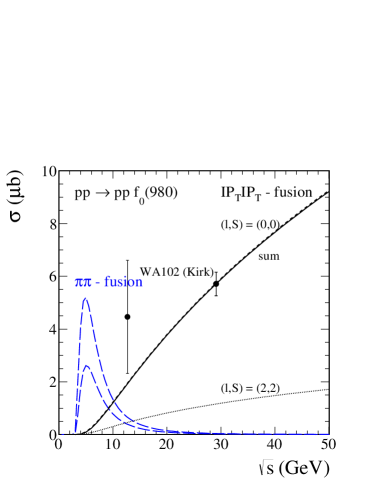
(a) (b)
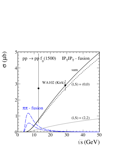
(c)

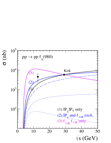
Figure 3: The integrated cross section as a function of the proton-proton center-of-mass energy for the $pp\to ppf_{0}(980)$ (panel (a)) and $pp\to ppf_{0}(1500)$ (panel (b)) reactions. We show data points obtained by the WA102 experiment kirk00 ; WA102_PLB462 . The two long-dashed lines peaked at $\sqrt{s}\approx$ 5-7 GeV correspond to pion-pion fusion contribution. The pomeron-pomeron fusion dominates at higher energies. In panels (a) and (b) we show the individual contributions to the cross section with $(l,S)=(0,0)$ (short-dashed line) and $(l,S)=(2,2)$ (dotted line). In panels (a) and (b) we show results when only the $I\!\!P_{T}I\!\!P_{T}$-fusion is included. In panel (c) the black solid line (1) presents the $I\!\!P_{T}I\!\!P_{T}$-fusion, the blue solid line (2) correspond to the results with tensor pomeron and $f_{2I\!\!R}$ exchanges (the long-dashed, dash-dotted and dotted lines present the $I\!\!P_{T}I\!\!P_{T}$, $I\!\!P_{T}f_{2I\!\!R}$ and $f_{2I\!\!R}f_{2I\!\!R}$ contributions, respectively). The violet solid line (3) presents the $f_{2I\!\!R}f_{2I\!\!R}$-fusion alone normalized to the total cross section from kirk00 as given in our Table 2.

In Fig. 4 we show the distribution in azimuthal angle $\phi_{pp}$ between outgoing protons for central exclusive $f_{0}(1370)$ meson production by the fusion of two tensor (solid line) and vector (long-dashed line) pomerons at $\sqrt{s}=29.1$ GeV. The results of the two models of pomeron exchanges are compared with the WA102 data. The tensorial pomeron with the $(l,S)=(0,0)$ coupling alone already describes the azimuthal angular correlation for $f_{0}(1370)$ meson reasonable well. The vectorial pomeron with the $(l,S)=(0,0)$ term alone is disfavoured here. The preference of the $f_{0}(1370)$ for the $\phi_{pp}\approx\pi$ domain in contrast to the enigmatic $f_{0}(980)$ and $f_{0}(1500)$ scalars has been observed by the WA102 Collaboration WA102_PLB462 .

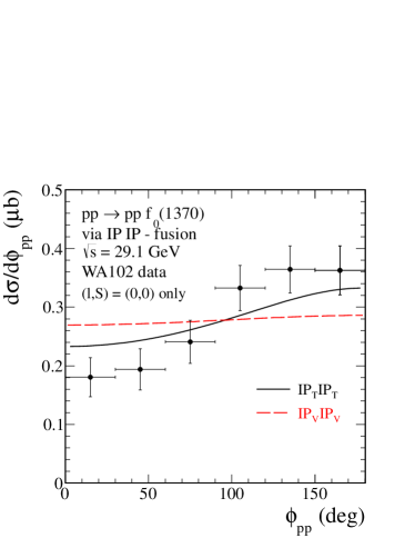
Figure 4: The distribution in azimuthal angle between the outgoing protons for central exclusive $f_{0}(1370)$ meson production by a fusion of two tensor (solid line) and vector (long-dashed line) pomerons at $\sqrt{s}=29.1$ GeV. The WA102 experimental data points from WA102_PLB462 have been normalized to the total cross section from kirk00 as given in our Table 2. The corresponding $I\!\!PI\!\!PM$ coupling constants are as given in Table 3.

The distributions in azimuthal angle $\phi_{pp}$ between the outgoing protons for the central exclusive production of the mesons $f_{0}(980)$ and $f_{0}(1500)$ at $\sqrt{s}=29.1$ GeV are shown in Figs. 5 and 6, respectively. We compare results obtained by the fusion of two pomerons (the tensor pomeron exchanges are shown in panels (a) - (c) and the vector pomeron exchanges are shown in panels (d) - (f)) with the data measured by the WA102 Collaboration in WA102_PLB462 (the black filled points) and WA102_PLB467 (the blue circle points). In the left panels we show the $\phi_{pp}$ distribution without experimental cuts, the middle panels show the $\phi_{pp}$ distribution for $|t_{1}t_{2}|\leqslant 0.01$ GeV⁴ and the right panels show the corresponding distribution for $|t_{1}t_{2}|\geqslant 0.08$ GeV⁴. Note that in WA102_PLB462 and WA102_PLB467 only normalised distributions are given. We have multiplied these distributions with the mean value of the total cross sections from Table 2 for panels (a) and (d). For panels (b), (c), (e), and (f) we have multiplied the normalised data distributions given in WA102_PLB467 with the cross sections obtained from our calculations in the tensorial and vectorial pomeron models, respectively; see Table 3. These normalisation factors are different for the $I\!\!P_{T}$ and $I\!\!P_{V}$ cases. Therefore, also the “data” shown in panels (b) and (e), as well as in (c) and (f), are different. Also note that the difference in the data from WA102_PLB462 and WA102_PLB467 shown in panels (a) and (d) has an experimental origin, as far as the authors can tell. Correspondingly, in the panels (a) the black filled and the blue circle experimental points are described by the tensorial pomeron exchanges for different values of the two $(l,S)$ contributions. For the $f_{0}(980)$ (Fig. 5(a)) we obtain these coupling constants as $(g_{I\!\!PI\!\!PM}^{\prime},g_{I\!\!PI\!\!PM}^{\prime\prime})=(0.788,4)$ (the black solid line) and $(g_{I\!\!PI\!\!PM}^{\prime},g_{I\!\!PI\!\!PM}^{\prime\prime})=(0.75,5.5)$ (the blue solid line), respectively. The values of the couplings for $f_{0}(1500)$ production shown in Fig. 6(a) are $(g_{I\!\!PI\!\!PM}^{\prime},g_{I\!\!PI\!\!PM}^{\prime\prime})=(1.22,6)$ (the black solid line) and $(g_{I\!\!PI\!\!PM}^{\prime},g_{I\!\!PI\!\!PM}^{\prime\prime})=(1,10)$ (the blue solid line), respectively. From our results we conclude that both $(l,S)$ contributions are necessary if the distributions in azimuthal angle are to be described accurately. The $(l,S)=(2,2)$ contribution increases the cross section at large $\phi_{pp}$ while decreasing it for small $\phi_{pp}$. The panels (d) - (f) show the results obtained for two vector pomerons coupling to the mesons. The curves present contributions from different $(l,S)$ couplings collected in Table 3. In the panel (d) of Fig. 5 ($f_{0}(980)$ production) the black long-dashed line corresponds to $(g_{I\!\!PI\!\!PM}^{\prime},g_{I\!\!PI\!\!PM}^{\prime\prime})=(0.27,0.8)$ and the blue long-dashed line to $(g_{I\!\!PI\!\!PM}^{\prime},g_{I\!\!PI\!\!PM}^{\prime\prime})=(0.24,1.5)$. For $f_{0}(1500)$ production shown in panel (d) of Fig. 6 the black long-dashed line corresponds to $(g_{I\!\!PI\!\!PM}^{\prime},g_{I\!\!PI\!\!PM}^{\prime\prime})=(0.208,0.725)$, the blue long-dashed line to $(g_{I\!\!PI\!\!PM}^{\prime},g_{I\!\!PI\!\!PM}^{\prime\prime})=(0.164,1.5)$. With these values we are able to describe well the black filled and blue circle experimental points, respectively. For panels (e) and (f) we have multiplied the normalised data from WA102_PLB467 with the cross sections obtained from our calculations. In panels (g) - (i) the results obtained with the two models of pomeron are compared. From Figs. 5 and 6 we conclude that, especially for $|t_{1}t_{2}|\geqslant 0.08$ GeV⁴, the tensorial pomeron ansatz is in better (qualitative) agreement with the data than the vectorial ansatz. But let us recall that for panels (b), (c), (e), and (f) the normalisation is taken from the models themselves for lack of experimental information.

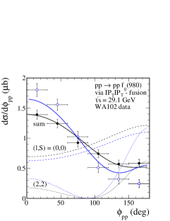
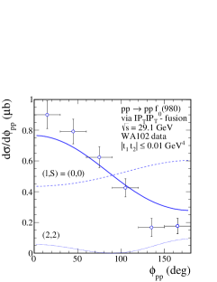
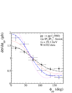
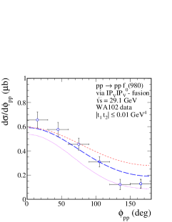
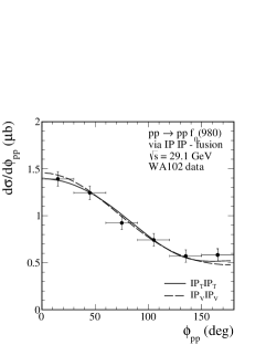
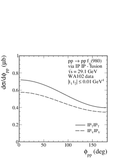
(a) (b) (c)
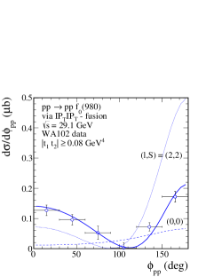
(d) (e) (f)
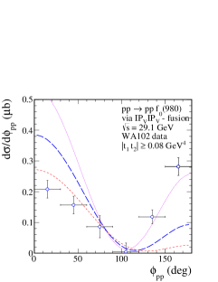
(g) (h) (i)

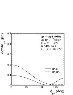
Figure 5: The distribution in azimuthal angle between outgoing protons for the central exclusive $f_{0}(980)$ meson production by the fusion of both tensor (panels (a) - (c)) and vector (panels (d) - (f)) pomerons at $\sqrt{s}=29.1$ GeV. Results in the left panels and the WA102 data points from WA102_PLB462 (black points) and from WA102_PLB467 (blue points) have been normalized to the mean value of the total cross section given in Table 2, obtained from Ref. kirk00 . The $\phi_{pp}$ distributions have also been analysed in two intervals of $|t_{1}t_{2}|$ and compared with experimental data . These data are obtained from WA102_PLB467 with the normalisation calculated in the tensorial and vectorial pomeron models themselves. We show in panels (a) - (c) the results in the tensorial pomeron model. For tensorial pomeron the individual contributions to the cross sections with $(l,S)=(0,0)$ (short-dashed line) and $(l,S)=(2,2)$ (dotted line) are also shown. Panels (d) - (f) show the results obtained for the vectorial pomeron model. In panels (g) - (i) the results obtained in the two models of pomeron are compared.

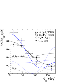
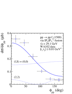
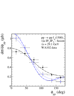
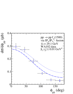
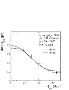
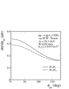
(a) (b) (c)
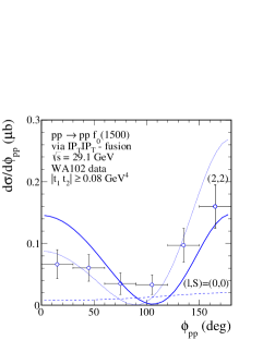
(d) (e) (f)
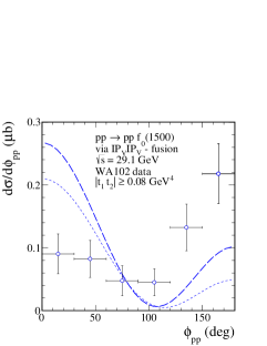
(g) (h) (i)

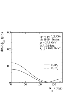
Figure 6: Same as Fig. 5, but for the central exclusive $f_{0}(1500)$ meson production.

At present we have calculated only so-called bare amplitudes which are subjected to absorption corrections. The absorption effects lead usually to a weak energy dependent damping of the cross sections. At the energy of the WA102 experiment ($\sqrt{s}=29.1$ GeV) the damping factor is expected to be at most of the order of 2 and should increase with rising collision energy. The absorption effects both in initial and final states have been considered in Ref. PRSG05 . It was stressed in Ref. PRSG05 that at the WA102 energies absorptive effects are not so significant and the azimuthal angle dependence looks like the “bare” one.

In Fig. 7 we show the distributions in transferred four-momentum squared $t$ between the initial and final protons at $\sqrt{s}=29.1$ GeV for $f_{0}(980)$, $f_{0}(1370)$, and $f_{0}(1500)$ mesons. While for $f_{0}(1370)$ the $(l,S)=(0,0)$ coupling is sufficient (see discussion of azimuthal correlations in Fig. 4) for $f_{0}(980)$ and $f_{0}(1500)$ both the $(0,0)$ and $(2,2)$ couplings are included. A different structure of the central vertex for vector and tensor leads to a difference in $t$ distribution; see panels (a) - (c). The difference seems, however, too small to be verified experimentally. In addition, in panels (a) - (c) we compare distributions obtained for two types of pomeron-pomeron-meson form factors of the exponential form (53) and the monopole form (51). The calculations with the exponential form factor (53) and for the cut-off parameter $\Lambda_{E}^{2}=0.6$ GeV² give a sizeable decrease of the cross sections at large $|t|$. In panel (d) we show contributions for two tensor pomerons (the line (1)) and $f_{2I\!\!R}$ reggeons (the line (3)) exchanges alone, since the contribution with tensorial pomeron and $f_{2I\!\!R}$ reggeon is included as well (the line (2)). We conclude that the $f_{2I\!\!R}f_{2I\!\!R}$ component alone does not describe the WA102 data. In panels (e) and (f) we show a decomposition of the $t$-distribution into $(0,0)$ and $(2,2)$ components for the tensor pomeron exchanges. At $t=0$ the $(2,2)$ component vanishes, in contrast to the $(0,0)$ component. Therefore, the latter dominates at small $|t|$. As previously, we show lines for the two parameter sets obtained from the fits to the two different experimental azimuthal angular correlations (see panels (a) in Figs. 5 and 6).

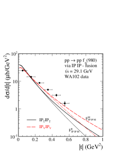
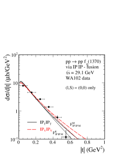
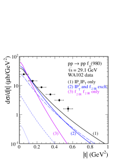
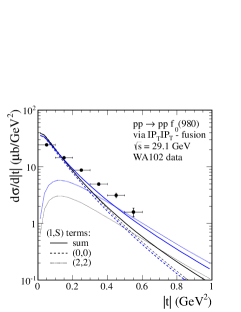
(a) (b) (c)
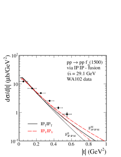
(d) (e) (f)

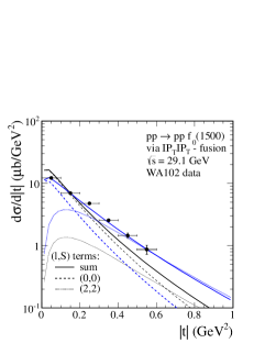
Figure 7: The $t$ distributions for $f_{0}(980)$ (panels (a), (d) and (e)), $f_{0}(1370)$ (panel (b)), and $f_{0}(1500)$ (panels (c) and (f)) meson production at $\sqrt{s}=29.1$ GeV. The WA102 experimental data points from WA102_PLB462 have been normalized to the mean value of the total cross sections given in Table 2 as obtained from kirk00 . In panels (a) - (c) the results for the fusion of two tensor (solid line) and vector (long-dashed line) pomerons are shown. The lower lines correspond to calculations with the exponential form factor (53) for the cut-off parameter $\Lambda_{E}^{2}=0.6$ GeV², the upper lines to calculations with the monopole form factor (51) for $\Lambda_{0}^{2}=0.5$ GeV². In panel (d) the black solid line (1) corresponds to the $I\!\!P_{T}I\!\!P_{T}$-fusion only, the blue solid line (2) corresponds to the tensor pomeron and $f_{2I\!\!R}$ exchanges (the long-dashed, dash-dotted and dotted lines present the $I\!\!P_{T}I\!\!P_{T}$, $I\!\!P_{T}f_{2I\!\!R}$ ($f_{2I\!\!R}I\!\!P_{T}$) and $f_{2I\!\!R}f_{2I\!\!R}$ contributions, respectively), and the violet solid line (3) presents the $f_{2I\!\!R}f_{2I\!\!R}$-fusion alone normalized to the integrated cross section from kirk00 ; see Table 2. In panels (e) and (f) we show the individual spin contributions to the cross sections with $(l,S)=(0,0)$ (short-dashed line) and $(l,S)=(2,2)$ (dotted line) as well as lines for the two sets of couplings fixed previously by comparison with the experimental azimuthal angular correlations (see panels (a) in Figs. 5 and 6).

In Fig. 8 we present different differential observables (in proton and meson transverse momenta as well as in the so-called “glueball filter variable” $dP_{\perp}$) at $\sqrt{s}=29.1$ GeV for the central exclusive production of three different scalar mesons, $f_{0}(980)$ (left panel), $f_{0}(1500)$ (middle panel) and $f_{0}(1370)$ (right panel). As explained in the figure caption we show results for both tensor (solid line) and vector (long-dashed line) pomerons as well as the individual spin $(l,S)$ contributions for tensor pomeron only. The coherent sum of the $(0,0)$ and $(2,2)$ components is shifted to smaller $dP_{\perp}$ with respect to the $(0,0)$ component alone. This seems to be qualitatively consistent with the WA102 Collaboration result presented in Table 2 of Ref. kirk00 . Further studies how different scalar mesons are produced as a function of $dP_{\perp}$ will be presented in the next section; see discussion of Fig. 18. For meson transverse momentum one can see a shift in the opposite direction.

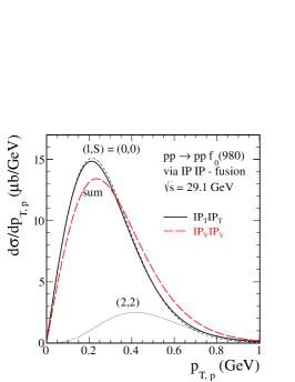
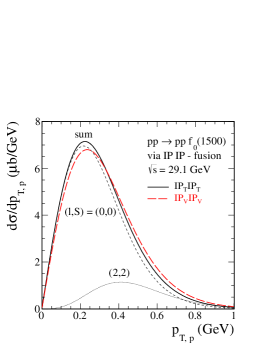
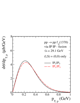
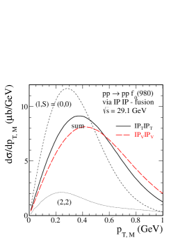
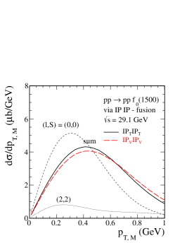
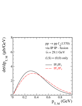
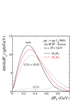
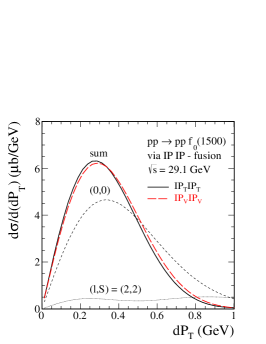
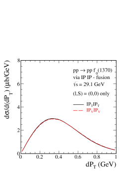
Figure 8: The different differential observables for the central exclusive production of $f_{0}(980)$ (left panel), $f_{0}(1500)$ (central panel) and $f_{0}(1370)$ (right panel) mesons by the fusion of two tensor (solid line) and vector (long-dashed line) pomerons at $\sqrt{s}=29.1$ GeV. The results have been normalized to the mean value of the total cross sections given in Table 2. For the tensorial pomeron case we show the individual spin contributions to the cross sections with $(l,S)=(0,0)$ (short-dashed line) and $(l,S)=(2,2)$ (dotted line).

In Fig. 9 we show distributions in transverse momenta of protons, mesons and in the $dP_{\perp}$ for the $f_{0}(980)$ meson production. The three tensorial scenarios of meson production, as in Fig. 7 (b), are presented. One conclusion is that the $f_{2I\!\!R}f_{2I\!\!R}$ contribution, indicated in the figure as curve (3), does not give the expected $dP_{\perp}$ distribution as in Table 2 of Ref. kirk00 .

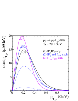
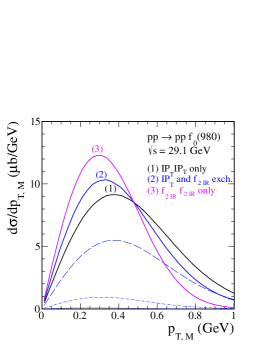
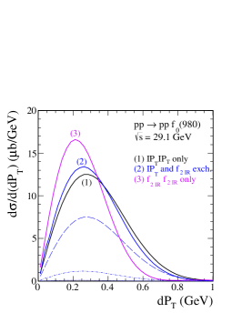
Figure 9: Different differential observables for the central exclusive production of $f_{0}(980)$ meson at $\sqrt{s}=29.1$ GeV. The results have been normalized to the mean value of the total cross section given in Table 2. The black solid line (1) corresponds to the $I\!\!P_{T}I\!\!P_{T}$-fusion, the blue solid line (2) to the results with tensor pomeron and $f_{2I\!\!R}$ exchanges (the long-dashed, dash-dotted and dotted lines present the $I\!\!P_{T}I\!\!P_{T}$, $I\!\!P_{T}f_{2I\!\!R}$, and $f_{2I\!\!R}f_{2I\!\!R}$ contributions, respectively), and the violet solid line (3) presents the $f_{2I\!\!R}f_{2I\!\!R}$-fusion alone normalized to the integrated cross section from kirk00 ; see Table 2.

In Fig. 10 we show distributions in rapidity $\mathrm{y}_{M}$ of $f_{0}(980)$ and $f_{0}(1500)$ mesons and the corresponding distributions in pseudorapidity $\eta_{M}$ at $\sqrt{s}=29.1$ GeV. In these observables both $(l,S)$ components and their coherent sum have similar shape. The minimum in the pseudorapidity distributions can be understood as a kinematic effect; see Appendix D. In addition, for the $f_{0}(980)$ meson production we have included the tensorial $f_{2I\!\!R}$ contributions; see the central panels. The $I\!\!P_{T}I\!\!P_{T}$ and the $f_{2I\!\!R}f_{2I\!\!R}$ exchanges contribute at midrapidity of the meson, while the $I\!\!P_{T}f_{2I\!\!R}$ and $f_{2I\!\!R}I\!\!P_{T}$ exchanges at backward and forward meson rapidity, respectively. The interference of these components in the amplitude produces enhancements of the cross section at large $|\mathrm{y}_{M}|$ and $|\eta_{M}|$.

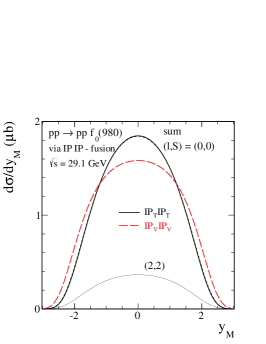
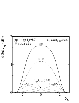
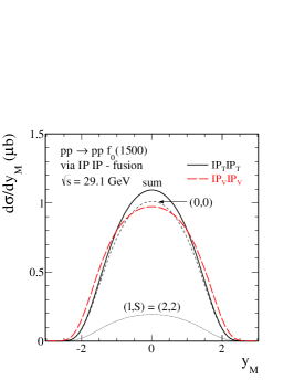
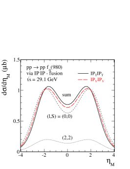
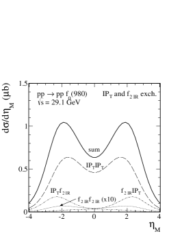
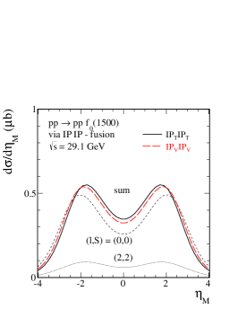
Figure 10: Rapidity and pseudorapidity distributions of $f_{0}(980)$ and $f_{0}(1500)$ produced by the fusion of two tensor (solid line) and vector (long-dashed line) pomerons at $\sqrt{s}=29.1$ GeV. The results have been normalized to the mean value of the total cross sections given in Table 2. For tensorial pomeron the individual contributions of $(l,S)=(0,0)$ (short-dashed line), $(l,S)=(2,2)$ (dotted line), and their coherent sum (solid line) are shown. In the center panels we show the results for the $f_{0}(980)$ meson production with the tensorial $f_{2I\!\!R}$ contributions included.

In Fig. 11 we show the distribution in Feynman-$x_{F}$ for the central exclusive $f_{0}(980)$ meson (the only available experimentally) production at $\sqrt{s}=29.1$ GeV. The good agreement of the $I\!\!P_{T}I\!\!P_{T}$-fusion result (see the solid line in the left panel) with the WA102 data suggests that for the tensor pomeron model the pomeron-reggeon and reggeon-reggeon contributions are small.

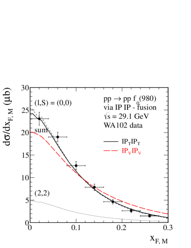
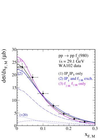
Figure 11: The $x_{F,M}$ distribution for the central exclusive $f_{0}(980)$ meson production at $\sqrt{s}=29.1$ GeV. The WA102 experimental data points from CloseKirk2000 have been normalized to the mean values of the total cross section given in Table 2. In the left panel we show the results obtained by the fusion of two tensor pomerons. In addition, the individual $(l,S)=(0,0)$ and $(2,2)$ contributions denoted by the short-dashed and dotted lines, respectively, are presented. In the right panel the black solid line (1) corresponds to the $I\!\!P_{T}I\!\!P_{T}$-fusion, the blue solid line (2) to the results with tensor pomeron and $f_{2I\!\!R}$ exchanges (the long-dashed, dash-dotted and dotted lines present the $I\!\!P_{T}I\!\!P_{T}$, $I\!\!P_{T}f_{2I\!\!R}$ and $f_{2I\!\!R}f_{2I\!\!R}$ (enlarged by a factor $20$) contributions, respectively), and the violet solid line (3) presents the $f_{2I\!\!R}f_{2I\!\!R}$-fusion contribution alone normalized to the mean value of the total cross section given in Table 2.

Up to now we have observed some differences of the results for $(l,S)=(0,0)$ and $(2,2)$ couplings. The differences can be made better visible in two-dimensional distributions. In Fig. 12 we show, as an example, two-dimensional distributions in ($dP_{\perp},\phi_{pp}$). We show results for the fusion of two tensor (left panels) and two vector (right panels) pomerons. In panels (a) and (b) we show the results for both $(l,S)$ components added coherently. In panels (c, d) and (e, f) we show the individual components for $(l,S)=(0,0)$ and $(2,2)$, respectively. The distributions for both cases are very different. By comparing panels (a) and (b) to panels (c, e) and (d, f), respectively, we see that the interference effects are rather large.

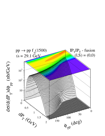
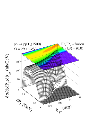
(a) (b) (c) (d) (e) (f)

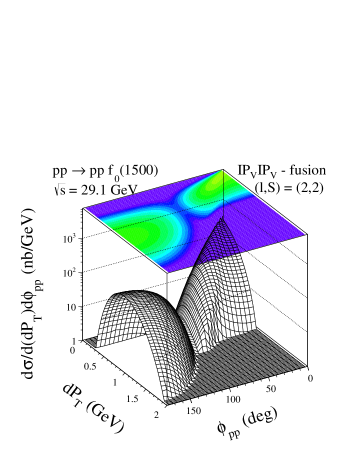
Figure 12: Distributions in ($dP_{\perp},\phi_{pp}$) for the central exclusive $f_{0}(1500)$ meson production via the tensorial (left panels) and vectorial (right panels) pomeron exchanges at $\sqrt{s}=29.1$ GeV. The individual contributions of $(l,S)=(0,0)$ (panels (c) and (d)) and $(l,S)=(2,2)$ (panels (e) and (f)) are shown separately.

III.2 Pseudoscalar meson production

We turn now to the presentation of our results for pseudoscalar mesons. It is known that the $\eta$ and $\eta^{\prime}$ mesons, the isoscalar members of the nonet of the lightest pseudoscalar mesons, play an important role in the understanding of various aspects of nonperturbative effects of QCD; see for instance DRB12 . The $\eta^{\prime}$-meson being dominantly a ($\alpha\ket{s\bar{s}}+\beta\ket{gg}$) state, with presence of a sizeable gluonic component Kroll , is particularly interesting for our study as here the pomeron-pomeron fusion should be the dominant mechanism in central production. For central production of the $\eta$ meson the situation may be more complicated and requires consideration of additional $f_{2I\!\!R}$ reggeon exchanges KMV99 ; KMV00 . In contrast to $\eta^{\prime}$ production, no good fit with (tensorial or vectorial) pomeron-pomeron component only is possible for the $\eta$ meson production. Therefore we have decided to include in addition $f_{2I\!\!R}I\!\!P$, $I\!\!Pf_{2I\!\!R}$ and $f_{2I\!\!R}f_{2I\!\!R}$ contributions into our analysis. The corresponding coupling constants were roughly fitted to existing experimental differential distributions (some specific details will be given when discussing differential distributions); see Table 4. We recall from the discussion in Section II.2 that for the tensorial pomeron two $I\!\!PI\!\!P\tilde{M}$ couplings, $(l,S)=(1,1)$ and $(3,3)$, are possible. For the vectorial pomeron we have only $(l,S)=(1,1)$. As will be discussed below in addition to pomeron-pomeron fusion the inclusion of secondary reggeons is required for a simultaneous description of $d\sigma/d\phi_{pp}$, $d\sigma/dt$ and $d\sigma/dx_{F}$ experimental data for the $\eta$ production.

Table 4: The values of the pomeron-pomeron-meson $\tilde{M}$ coupling constants of the two models of the pomeron exchanges which are approximately fitted to reproduce the correct normalization, see Table 2, and shapes of differential distributions of the WA102 experiment. In addition, the cross sections (in $\mu$b) for the individual $(l,S)$ contributions at $\sqrt{s}=29.1$ GeV are shown.

Meson	Exchanges	$g_{I\!\!PI\!\!P\tilde{M}}^{\prime}$	$g_{I\!\!PI\!\!P\tilde{M}}^{\prime\prime}$	$\sigma$ ($\mu$b) at $\sqrt{s}=29.1$ GeV
$\tilde{M}$		$(1,1)$ term	$(3,3)$ term	$(1,1)$	$(3,3)$	total
$\eta$	$I\!\!P_{T}I\!\!P_{T}$, $I\!\!P_{T}f_{2I\!\!R}$, $f_{2I\!\!R}I\!\!P_{T}$, $f_{2I\!\!R}f_{2I\!\!R}$	0.8, 2.45, 2.45, 2	1.4, 4.29, 4.29, 3.5	5.05	0.85	3.85
	$I\!\!P_{T}I\!\!P_{T}$	2	2.25	4.83	0.55	3.85
	$I\!\!P_{V}I\!\!P_{V}$	8.47	-	3.86	–	–
$\eta^{\prime}$	$I\!\!P_{T}I\!\!P_{T}$	2.61	1.5	1.86	0.05	1.71
	$I\!\!P_{V}I\!\!P_{V}$	6.08	-	1.72	–	–

In Fig. 13 we present energy dependences of the cross sections for $\eta$ (panels (a) and (c)) and $\eta^{\prime}$ (panels (b) and (d)) meson production. It was argued in Ref. KMV00 that $f_{2I\!\!R}$-pomeron and pomeron-$f_{2I\!\!R}$ exchanges could be important for both $\eta$ and $\eta^{\prime}$ central production. For comparison, we show the results where $f_{2I\!\!R}$ exchanges are included for $\eta$ production. We observe a large interference of different components in the amplitude (the long-dashed line denotes the pomeron-pomeron component, the dash-dotted line – $f_{2I\!\!R}$-pomeron (or pomeron-$f_{2I\!\!R}$) component, and the dotted line – $f_{2I\!\!R}f_{2I\!\!R}$ component). In the diffractive mechanism we use vertex form factor given by Eqs. (51) and (52). Our results have been normalized to the experimental total cross sections given in Table 2 and take into account (see the dash-dotted line in panels (a) and (b)) the limited Feynman-$x_{F}$ domain $0\leqslant x_{F,M}\leqslant 0.1$ for the corresponding data points; see WA102_PLB427 . Moreover, at lower energies we can expect large contributions from $\omega$-$\omega$ exchanges due to the large coupling of the $\omega$ meson to the nucleon. The dashed bottom and upper lines at low energies represent the $\omega\omega$-contribution calculated with the monopole (54) and exponential (55) form factors, respectively. In the case of meson exchanges we use values of the cut-off parameters $\Lambda_{E}=\Lambda_{M}=1.4$ GeV. We have taken rather maximal $\Lambda_{E}$ and $\Lambda_{M}$ in order to obtain an upper limit for this contribution. As explained in Section II.2 at higher subsystem squared energies $s_{13}$ and $s_{23}$ the meson exchanges are corrected to obtain the high energy behaviour appropriate for reggeon exchange, cf. Eq. (29).

In both panels (a) and (b) the dotted line represents the $\omega_{I\!\!R}\omega_{I\!\!R}$-contribution calculated with coupling constant $g_{\omega_{I\!\!R}\omega_{I\!\!R}\tilde{M}}=60$. Due to charge-conjugation invariance the $\eta$ and $\eta^{\prime}$ cannot be produced by $\omega$-pomeron exchange and isospin conservation forbids $\rho$-pomeron exchange. In the region of small momentum transfer squared the contribution from other processes such as photon-(vector meson) and photon-photon fusion is possible CEF98 , but the cross section is expected to be several orders of magnitude smaller SPT07 ; KN98 than for the double pomeron processes.

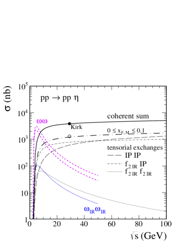
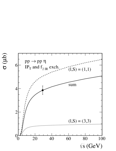
(a) (b)
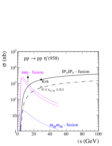
(c) (d)

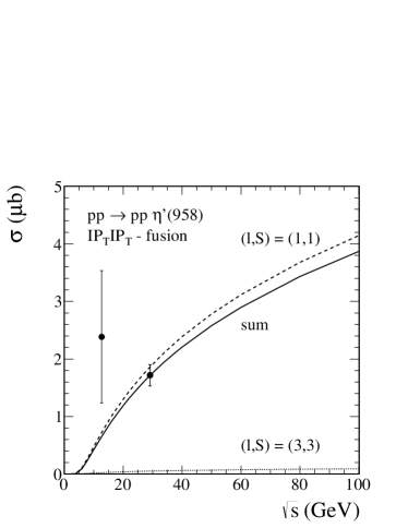
Figure 13: Cross section for the $pp\to pp\eta$ (panel a) and $pp\to pp\eta^{\prime}(958)$ (panel b) reaction as a function of proton-proton center-of-mass energy $\sqrt{s}$. The experimental data are from the WA102 experiment at $\sqrt{s}=29.1$ GeV; see Table 2 obtained from kirk00 , and for the Feynman-$x_{F}$ interval $0\leqslant x_{F,M}\leqslant 0.1$ WA102_PLB427 . There is also a data point at $\sqrt{s}=12.7$ GeV obtained from Table 1. The $\omega\omega$-fusion contribution is important only at lower energies while tensorial pomeron fusion contribution dominates at higher energies. In the diffractive mechanism we use vertex form factor (51) and the value of coupling constants collected in Table 4. For the $\eta$ meson production the tensorial contributions of $I\!\!PI\!\!P$, $f_{2I\!\!R}I\!\!P$ ($I\!\!Pf_{2I\!\!R}$) and $f_{2I\!\!R}f_{2I\!\!R}$ exchanges were included. Their coherent sum is shown by the solid line. For the $\eta^{\prime}$ meson production the solid line represents the cross section obtained via tensor pomeron exchanges only. For comparison, in the panels (c) and (d), we show the individual contributions to the cross section with $(l,S)=(1,1)$ (short-dashed line) and $(l,S)=(3,3)$ (dotted line).

In Fig. 14 we show the cross section as a function of the azimuthal angle $\phi_{pp}$ between the transverse momentum vectors of the two outgoing protons; see (105). The vertex form factor (51) was used in calculations. For tensor pomeron the strengths of the $(l,S)=(1,1)$ and $(3,3)$ were adjusted to roughly reproduce the azimuthal angle distribution. The contribution of the $(1,1)$ component alone is not able to describe the azimuthal angular dependence (see panel (b)). For both models the theoretical distributions are somewhat skewed with respect to a simple $\sin^{2}(\phi_{pp})$ dependence as obtained e.g. from vector-vector-pseudoscalar coupling alone without phase space effects. The small deviation in this case is due to phase space angular dependence. The matrix element squared itself is proportional to $\sin^{2}(\phi_{pp})$. For comparison, the dash-dotted line in the panel (c) corresponds to $\gamma\gamma$-fusion for the $\eta^{\prime}$ production calculated as in SPT07 .

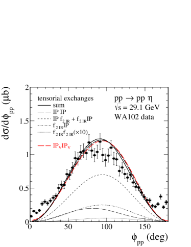
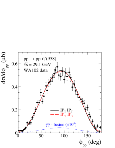
(a) (b)
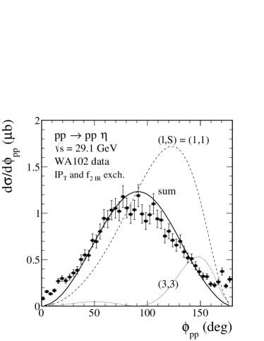
(c) (d)

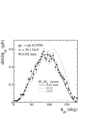
Figure 14: Differential cross section $d\sigma/d\phi_{pp}$ for the $pp\to pp\eta$ and $pp\to pp\eta^{\prime}(958)$ reactions at $\sqrt{s}=29.1$ GeV. The WA102 experimental data from WA102_PLB427 have been normalized to the mean values of the total cross sections given in Table 2. Panel (a) shows the results for $\eta$ production. The solid line is the result for the tensorial pomeron including two $(l,S)$ couplings as well as $f_{2I\!\!R}I\!\!P$, $I\!\!Pf_{2I\!\!R}$, and $f_{2I\!\!R}f_{2I\!\!R}$ exchanges. The red long-dashed line corresponds to vector pomeron exchange only and $(l,S)=(1,1)$ coupling. In panel (b) the two $(l,S)$ contributions from the tensorial pomeron exchanges and their total are shown. In panel (c) we show the results for $\eta^{\prime}$ production for the case of tensor and vector pomeron exchanges as well as the $\gamma\gamma$-fusion enlarged by a factor $10^{4}$. Panel (d) shows the results for $I\!\!P_{T}I\!\!P_{T}$-fusion.

In Fig. 15 we present distribution in $|t_{1}|$ and $|t_{2}|$, which are, of course identical. Therefore we label them by $|t|$. As can be seen from panels (a) and (c) the results for the tensorial exchanges give a better description of $t$ distribution than the vector pomeron exchanges. The $t$-dependence of $\eta$ and $\eta^{\prime}$ production is very sensitive to the form factor $F_{I\!\!PI\!\!PM}(t_{1},t_{2})$, cf. (51), in the pomeron-pomeron-meson vertex.

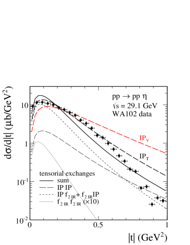
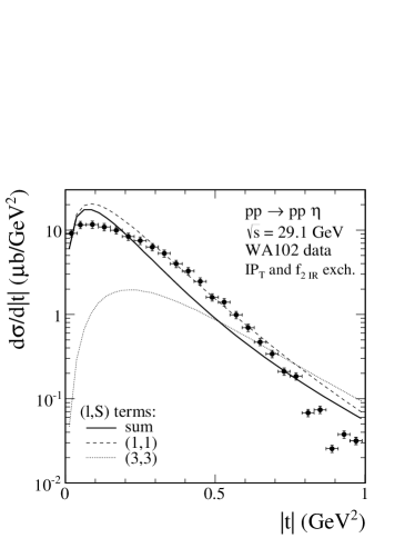
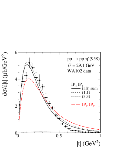
(a) (b) (c) (d)

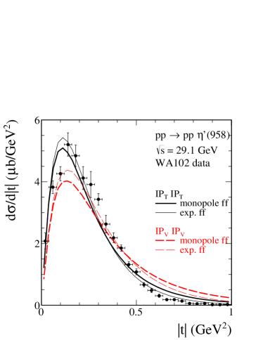
Figure 15: Differential cross section $d\sigma/d|t|$ for the $pp\to pp\eta$ (panels (a) and (b)) and $pp\to pp\eta^{\prime}$ (panels (c) and (d)) reactions at $\sqrt{s}=29.1$ GeV. The WA102 experimental distributions from WA102_PLB427 have been normalized to the mean values of the total cross sections given in Table 2. The solid line corresponds to the model with tensorial pomeron while the dashed line to the model with vectorial pomeron. For $\eta$ production the $f_{2I\!\!R}$ exchanges were included in addition. In the present calculations we use vertex form factor given by Eqs. (51) and (52). For comparison, in panel (d), we also show the results for exponential form factor (53) and for $\Lambda_{E}^{2}=0.7$ GeV².

In Fig. 16 we present the $d\sigma/dx_{F}$ distribution. We see that $\eta$ (panels (a) and (b)) and $\eta^{\prime}$ (panels (c) and (d)) meson distributions are peaked at $x_{F,M}\approx 0$, which is consistent with the dominance of the pomeron-pomeron exchange. In the calculations we use the pomeron-pomeron-meson couplings collected in Table 4. For the description of the $\eta$ production in the case of the tensorial pomeron the $f_{2I\!\!R}$ exchanges in the amplitude were included. In panel (a) the solid line corresponds to the model with tensorial pomeron plus $f_{2I\!\!R}$ exchanges and the long-dashed line to the model with vectorial pomeron. The enhancement of the $\eta$ distribution at larger values of $x_{F,M}$ can be explained by significant $f_{2I\!\!R}$-pomeron and pomeron-$f_{2I\!\!R}$ exchanges. As can be seen from panel (a) these contributions have maxima at $x_{F,M}\neq 0$. The corresponding couplings constants were fixed to differential distributions of the WA102 Collaboration WA102_PLB427 . In panel (b) we show for the tensorial pomeron the individual contributions to the cross section with $(l,S)=(1,1)$ (the short-dashed line), $(l,S)=(3,3)$ (the dotted line), and their coherent sum (the solid line). In panel (c) we show the Feynman-$x_{F}$ distribution of the $\eta^{\prime}$ meson and the theoretical curves for $I\!\!P_{T}I\!\!P_{T}$ and $I\!\!P_{V}I\!\!P_{V}$ fusion, respectively. The diffractively scattered outgoing protons are placed at $x_{F}\approx\pm 1$; see panel (d).

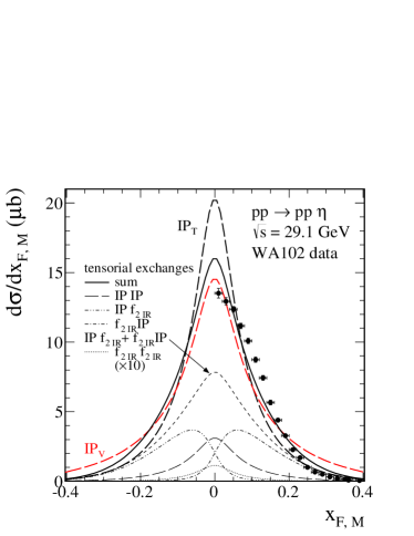
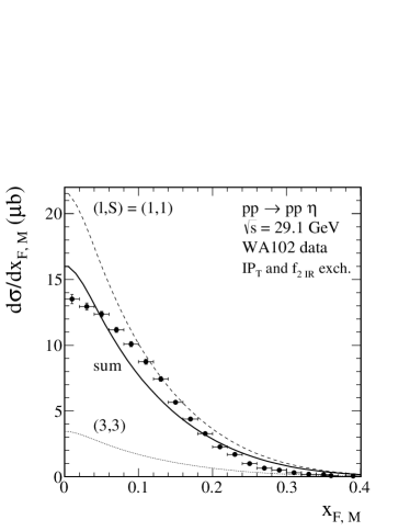
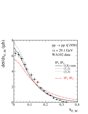
(a) (b) (c) (d)

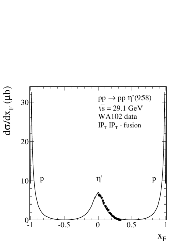
Figure 16: Differential cross section $d\sigma/dx_{F,M}$ for the $pp\to pp\eta$ (panels (a) and (b)) and $pp\to pp\eta^{\prime}$ (panels (c) and (d)) reactions at $\sqrt{s}=29.1$ GeV. The WA102 experimental data WA102_PLB427 are shown for comparison and have been normalized to the mean values of the total cross sections given in Table 2. In the present calculations we use vertex form factor (51) and two model of pomeron exchanges. In panel (a) the results for the tensorial pomeron and $f_{2I\!\!R}$ exchanges are shown; the pomeron-pomeron component peaks at $x_{F,M}=0$ (the long-dashed line), the pomeron-$f_{2I\!\!R}$ ($f_{2I\!\!R}$-pomeron) peaks at backward (forward) $x_{F,M}$, respectively, and the coherent sum of pomeron-$f_{2I\!\!R}$ and $f_{2I\!\!R}$-pomeron component effectively dominates in the central region of $x_{F,M}$ (the short-dashed line). In panels (b) and (c) we show the individual contributions to the cross section with $(l,S)=(1,1)$ (the short-dashed line), $(3,3)$ (the dotted line), and their coherent sum (the solid line). The long-dashed line in panel (c) corresponds to the model with vectorial pomeron. In panel (d) the $x_{F}$ distributions for $\eta^{\prime}$ (at $x_{F}=0$) and for the protons (at $x_{F}\to\pm 1$) are shown for $I\!\!P_{T}I\!\!P_{T}$ fusion.

In Fig. 17 we present distributions in meson transverse momentum $p_{\perp,M}$ and proton transverse momentum $p_{\perp,p}$. As already explained above for $\eta$ meson production we include in addition tensorial reggeon exchanges. Their individual contributions are shown in the left panels. In addition, we show the individual spin contributions to the cross section with $(l,S)=(1,1)$ (short-dashed line) and $(l,S)=(3,3)$ (dotted line). The coherent sum of $(1,1)$ and $(3,3)$ tensorial components is shifted with respect to the $(1,1)$ vectorial component alone.

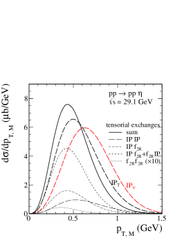
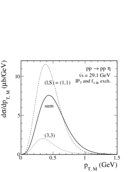
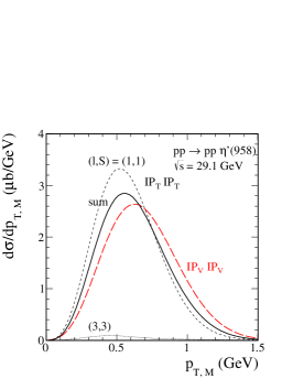
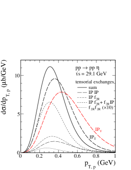
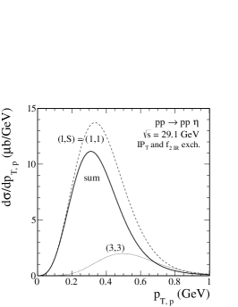
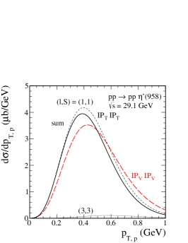
Figure 17: Differential cross sections $d\sigma/dp_{\perp,M}$ and $d\sigma/dp_{\perp,p}$ (the forward proton $p_{1}$) for the central exclusive $\eta$ and $\eta^{\prime}$ meson production at $\sqrt{s}=29.1$ GeV. The solid line corresponds to the model with tensorial pomeron while the dashed line to the model with vectorial pomeron. For $\eta$ production the $f_{2I\!\!R}$ exchanges in the amplitude were included in addition as discussed in the text. We show for the tensorial case also the individual contributions to the cross section with $(l,S)=(1,1)$ (short-dashed line) and $(l,S)=(3,3)$ (dotted line).

In Fig. 18 we present the “glueball variable” $dP_{\perp}$ distribution. Theoretical predictions of $dP_{\perp}$ seem to be qualitatively consistent with the WA102 data presented in Table 2 of Ref. kirk00 . We show results for the mesons of interest to us in Table 5. In addition, in Fig. 18(d), the ratio of production at small $dP_{\perp}$ to large $dP_{\perp}$ has been compared with the experimental results taken from kirk00 ; see also WA102_PLB462 . It can be observed that scalar mesons which could have a large ’gluonic component’ have a large value for this ratio. The fact that $f_{0}(1370)$ and $f_{0}(1500)$ have different $\phi_{pp}$ and $dP_{\perp}$ dependences confirms that these are not simply $J$ dependent phenomena. This is also true for the $J=2$ states, where the $f_{2}(1950)$ has a different $\phi_{pp}$ dependence compared to the $f_{2}(1270)$ and $f_{2}^{\prime}(1525)$ states; see Fig.5 of kirk00 . The $dP_{\perp}$ and $\phi_{pp}$ effects are in our present work understood as being due to the fact that in general more than one coupling structure, $I\!\!PI\!\!PM$ respectively $I\!\!PI\!\!P\tilde{M}$, is possible. It remains a challenge for theory to predict these coupling structures from calculations in the framework of QCD.

Table 5: Results of meson production as a function of $dP_{\perp}$ expressed as a percentage of its total contribution at the WA102 collision energy $\sqrt{s}=29.1$ GeV. The theoretical numbers quoted for $\eta$, $\eta^{\prime}$ and $f_{0}(1370)$ correspond to the coupling parameters given in Tables 4 and 3, respectively. For the $f_{0}(980)$ and $f_{0}(1500)$ the numbers (those in parentheses) correspond to the coupling parameters which fit in Figs. 5(a) and 6(a), respectively, the black filled (blue circle) points. See the discussion of these figures in the text. In the last column the ratios of $\frac{d\sigma/d(dP_{\perp}\leqslant\,0.2~{}\mathrm{GeV})}{d\sigma/d(dP_{\perp}\geqslant\,0.5~{}\mathrm{GeV})}$ are given. The experimental numbers are from Table 2 of Ref. kirk00 .

Meson	Exchanges	$dP_{\perp}\leqslant 0.2$ GeV	$0.2\leqslant dP_{\perp}\leqslant 0.5$ GeV	$dP_{\perp}\geqslant 0.5$ GeV	Ratio
$\eta$	$I\!\!P_{T}$ and $f_{2I\!\!R}$	3.0	46.8	50.1	0.06
	$I\!\!P_{T}I\!\!P_{T}$	1.8	33.4	64.8	0.03
	$I\!\!P_{V}I\!\!P_{V}$	1.1	21.0	77.8	0.01
	exp.	$6\pm 2$	$34\pm 2$	$60\pm 3$	$0.10\pm 0.03$
$\eta^{\prime}$	$I\!\!P_{T}I\!\!P_{T}$	1.4	28.3	70.4	0.02
	$I\!\!P_{V}I\!\!P_{V}$	1.2	22.1	76.7	0.02
	exp.	$3\pm 2$	$32\pm 2$	$64\pm 3$	$0.05\pm 0.03$
$f_{0}(980)$	$I\!\!P_{T}$ and $f_{2I\!\!R}$	25.3	59.2	15.2	1.67
	$I\!\!P_{T}I\!\!P_{T}$	22.7 (23.9)	57.9 (57.0)	19.3 (19.1)	1.18 (1.25)
	$I\!\!P_{V}I\!\!P_{V}$	19.3 (21.6)	54.9 (56.4)	25.9 (21.9)	0.74 (0.99)
	exp.	$23\pm 2$	$51\pm 2$	$26\pm 3$	$0.88\pm 0.12$
$f_{0}(1370)$	$I\!\!P_{T}I\!\!P_{T}$	15.5	49.0	35.5	0.44
	$I\!\!P_{V}I\!\!P_{V}$	15.2	48.5	36.3	0.42
	exp.	$18\pm 4$	$32\pm 2$	$50\pm 3$	$0.36\pm 0.08$
$f_{0}(1500)$	$I\!\!P_{T}I\!\!P_{T}$	22.5 (23.7)	57.8 (54.3)	19.7 (22.0)	1.15 (1.07)
	$I\!\!P_{V}I\!\!P_{V}$	20.4 (22.4)	56.0 (54.9)	23.6 (22.7)	0.86 (0.99)
	exp.	$24\pm 2$	$54\pm 3$	$22\pm 4$	$1.05\pm 0.18$

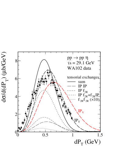
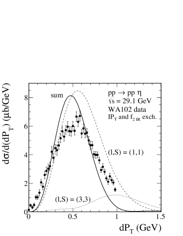
(a) (b)
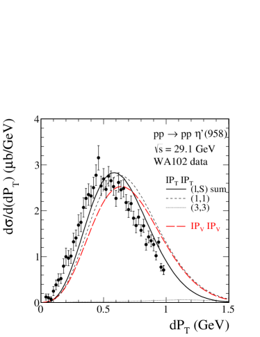
(c) (d)

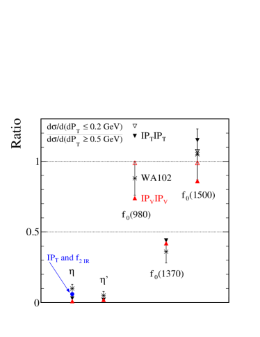
Figure 18: Differential cross section $d\sigma/d(dP_{\perp})$ for the central exclusive $\eta$ (panels (a) and (c)) and $\eta^{\prime}$ (panel (b)) mesons production at $\sqrt{s}=29.1$ GeV. The WA102 experimental distributions from WA102_PLB427 have been normalized to the mean values of the total cross sections from Table 2. Results for the tensorial and vectorial pomeron models are presented. For $\eta$ production the $f_{2I\!\!R}$ exchanges in the amplitude were included in addition. The $(l,S)$ contributions to the differential cross sections are also shown. Panel (d) shows the ratio of production at small $dP_{\perp}$ to large $dP_{\perp}$ for each pseudoscalar and scalar meson discussed in this paper and collected in Table 5. Experimental results for the ratio are taken from Table 2 of Ref. kirk00 . For the $f_{0}(980)$ and $f_{0}(1500)$ meson production we show results obtained for the two sets of $(l,S)$ contributions fitted to the experimental azimuthal angular correlations data shown in Figs. 5 and 6. For the $f_{0}(980)$ and $f_{0}(1500)$ the filled points correspond to $(g_{I\!\!P_{T}I\!\!P_{T}M}^{\prime},g_{I\!\!P_{T}I\!\!P_{T}M}^{\prime\prime})=(0.788,4)$ and $(1.22,6)$, the open points to $(g_{I\!\!P_{T}I\!\!P_{T}M}^{\prime},g_{I\!\!P_{T}I\!\!P_{T}M}^{\prime\prime})=(0.75,5.5)$ and $(1,10)$, respectively, see Table 3.

In Fig. 19 we show two-dimensional distributions in ($dP_{\perp},\phi_{pp}$) for the $\eta$ (left panels) and $\eta^{\prime}(958)$ (right panels) meson production in the fusion of two tensor pomerons. In panels (a) and (b) we show the result for $(l,S)$ components added coherently. In panels (c) - (d) and (e) - (f) we show the individual spin components for $(l,S)=(1,1)$ and $(3,3)$, respectively. By comparing panels (a) - (f) we infer that the interference effects are rather large.

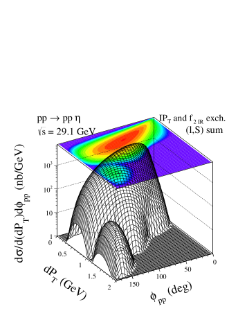
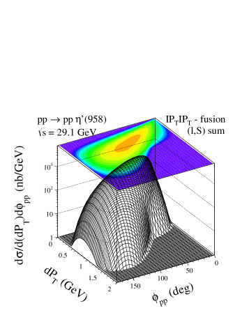
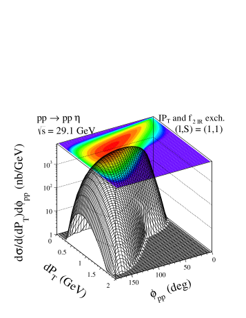
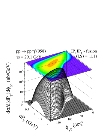
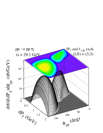
(a) (b) (c) (d) (e) (f)

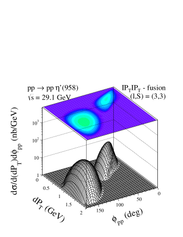
Figure 19: Distributions in ($dP_{\perp},\phi_{pp}$) for the $\eta$ (left panels) and $\eta^{\prime}(958)$ (right panels) meson production at $\sqrt{s}=29.1$ GeV, Results for $\eta$ meson correspond to the model with the tensor pomeron and $f_{2}$-reggeon exchanges while $\eta^{\prime}$ meson production to the model with tensorial pomeron only. The individual contributions of $(l,S)=(1,1)$ (panels (c) and (d)) and $(l,S)=(3,3)$ (panels (e) and (f)) are shown separately.

For completeness, differential distributions in the $\eta$ or $\eta^{\prime}$ rapidity (top panels) and pseudorapidity (bottom panels) are shown in Fig. 20 for the two models of the pomeron exchanges.

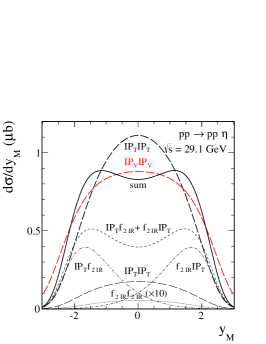
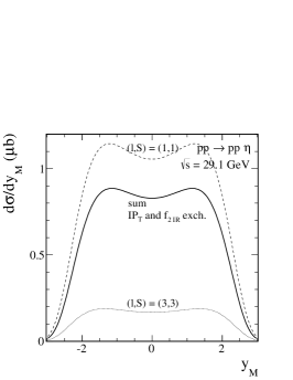
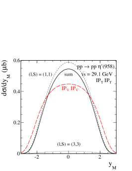
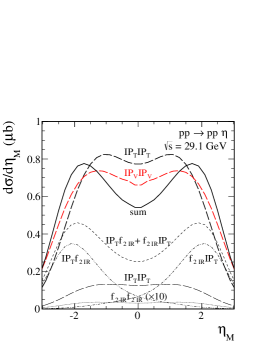
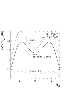
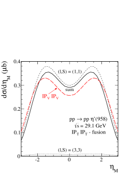
Figure 20: Differential cross section $d\sigma/d\mathrm{y}_{M}$ (top panels) and $d\sigma/d\eta_{M}$ (bottom panels) for the $\eta$ and $\eta^{\prime}$ production at $\sqrt{s}=29.1$ GeV. The solid line corresponds to the model with tensorial pomeron while the long-dashed line to the model with vectorial pomeron. The different lines correspond to the situation when all or only some components of the pomeron and $f_{2I\!\!R}$ exchanges in the amplitude are included (the pomeron-pomeron component dominates at midrapidities of $\mathrm{y}_{M}$ and the pomeron-reggeon (reggeon-pomeron) peaks at backward (forward) rapidities of $\mathrm{y}_{M}$, respectively).

IV Conclusions

We have analyzed proton-proton collisions with the exclusive central production of scalar and pseudoscalar mesons. We analyzed the predictions of two different models of the soft pomeron. The first one is the commonly used model with vectorial pomeron which is, however, difficult to be supported from a theoretical point of view. The second one is a recently proposed model of tensorial pomeron, which, in our opinion, has better theoretical foundations. We have presented formulae for corresponding pomeron-pomeron-meson vertices and amplitudes for the $pp\to pMp$ reaction. In general, different couplings with different orbital angular momentum and spin of two “pomeron particles” are possible. In most cases one has to add coherently amplitudes for two couplings. The corresponding coupling constants are not known and have been fitted to existing experimental data.

We have performed calculations of several differential distributions. We wish to emphasize that the tensorial pomeron can - at least - equally well describe experimental data on the exclusive meson production discussed here as the less theoretically justified vectorial pomeron frequently used in the literature. This has been illustrated for the production of several scalar and pseudoscalar mesons. The existing low-energy experimental data do not allow to clearly distinguish between the two models as the presence of subleading reggeon exchanges is at low energies very probable for many reactions. This seems to be the case for the $\eta$ meson production. In these cases we have included in our analysis also exchanges of subleading trajectories which improve the agreement with experimental data. Production of $\eta^{\prime}$ meson seems to be less affected by contributions from subleading exchanges.

Now we list some issues which deserve further studies but are beyond the scope of our present paper. For the resonances decaying e.g. into the $\pi\pi$ channel an interference of the resonance signals with the two-pion continuum has to be included in addition. This requires a consistent model of the resonances and the non-resonant background. It would be very interesting to see if the exchange of tensorial pomerons may modify differential distributions for the $\pi^{+}\pi^{-}$ continuum compared to the previous calculations LS10 ; LPS11 . Furthermore, absorption effects are frequently taken into account by simply multiplying cross sections with a gap survival factor. But absorption effects may also change the shapes of $t_{1}/t_{2}$, $\phi_{pp}$, etc. distributions. The deviation from “bare” distributions probably is more significant at high energies where the absorptive corrections should be more important. Consistent inclusion of these effects clearly goes beyond the scope of the present study where we have limited ourselves to simple Born term calculations at the WA102 collision energy. It would clearly be interesting to extend the studies of central meson production in diffractive processes to higher energies, where the dominance of the pomeron exchange can be better justified.

To summarise: our study of scalar and pseudoscalar meson production certainly shows the potential of these reactions for testing the nature of the soft pomeron. Pseudoscalar meson production could be of particular interest in this respect since there the distribution in the azimuthal angle $\phi_{pp}$ between the two outgoing protons may contain, for the tensorial pomeron, a term which is not possible for the vectorial pomeron; see the discussion after (15) and after (20) in Section II.2. Clearly, our study can be extended to the central production of other mesons like the $f_{2}(1270)$. We hope to come back to this issue in a future publication.

Our main aim with these studies is to provide detailed models for central meson production, for both the tensorial and the vectorial pomeron ansatz, where all measurable distributions of the particles in the final state can be calculated. The models contain only a few free coupling parameters to be determined by experiment. The hope is, of course, that future experiments will be able to select the correct soft pomeron model. In any case, our models should provide good “targets” for experimentalists to shoot at. Supposing that one model survives the experimental tests we have then the theoretical challenge of deriving the corresponding $I\!\!PI\!\!PM$ coupling constants from QCD.

Future experimental data on exclusive meson production at high energies should thus provide good information on the spin structure of the pomeron and on its couplings to the nucleon and the mesons. On the other hand, the low energy data could help in understanding the role of subleading trajectories. Several experimental groups, e.g. COMPASS COMPASS , STAR STAR , CDF CDF , ALICE ALICE , ATLAS SLTCS11 have the potential to make very significant contributions to this program aimed at understanding the coupling and the spin structure of the soft pomeron.

Acknowledgments We are indebted to C. Ewerz, K. Kochelev, and R. Schicker for useful discussions. Piotr Lebiedowicz is thankful to the Wilhelm and Else Heraeus - Foundation for warm hospitality during his stay at WE-Heraeus-Summerschool Diffractive and electromagnetic processes at high energies in Heidelberg when this work was completed. This work was partially supported by the Polish grants: DEC-2011/01/B/ST2/04535, DEC-2013/08/T/ST2/00165, and PRO-2011/01/N/ST2/04116.

Appendix A Tensorial pomeron

For the case of the tensorial pomeron the $I\!\!Ppp$ vertex and the $I\!\!P$ propagator read as follows, see talkN and EMN13 ,

$$i\Gamma_{\mu\nu}^{(I\!\!Ppp)}(p^{\prime},p)=-i3\beta_{I\!\!PNN}F_{1}\bigl{(}(p^{\prime}-p)^{2}\bigr{)}\left\{\frac{1}{2}\left[\gamma_{\mu}(p^{\prime}+p)_{\nu}+\gamma_{\nu}(p^{\prime}+p)_{\mu}\right]-\frac{1}{4}g_{\mu\nu}(p\!\!\!/^{\prime}+p\!\!\!/)\right\},\;\;\;\;\;\;\;$$ (30)

where $\beta_{I\!\!PNN}=1.87$ GeV^-1 and $p\!\!\!/=\gamma_{\mu}p^{\mu}$. The explicit factor 3 above counts the number of valence quarks in each proton. Following Donnachie and Landshoff DL we use in (30) for describing the proton’s extension the proton’s Dirac electromagnetic form factor $F_{1}(t)$. A good representation of this form factor is given by the dipole formula

$$F_{1}(t)=\frac{4m_{p}^{2}-2.79\,t}{(4m_{p}^{2}-t)(1-t/m_{D}^{2})^{2}}\,,$$ (31)

where $m_{p}$ is the proton mass and $m_{D}^{2}=0.71$ GeV² is the dipole mass squared.

The propagator of the tensor-pomeron exchange is given by

$$i\Delta_{\mu\nu,\kappa\lambda}^{(I\!\!P)}(s,t)=\frac{1}{4s}\left(g_{\mu\kappa}g_{\nu\lambda}+g_{\mu\lambda}g_{\nu\kappa}-\frac{1}{2}g_{\mu\nu}g_{\kappa\lambda}\right)\left(-is\alpha^{\prime}_{I\!\!P}\right)^{\alpha_{I\!\!P}(t)-1}\,;$$ (32)

see EMN13 . Here the pomeron trajectory $\alpha_{I\!\!P}(t)$ is assumed to be of standard form, see for instance DDLN , that is, linear in $t$ and with intercept slightly above 1:

$$\alpha_{I\!\!P}(t)=\alpha_{I\!\!P}(0)+\alpha^{\prime}_{I\!\!P}\,t\,,$$

$$\alpha_{I\!\!P}(0)=1.0808,\quad\alpha^{\prime}_{I\!\!P}=0.25\;\mathrm{GeV}^{-2}\,.$$ (33)

The tensor-pomeron propagator fulfils the following relations

$$\Delta_{\mu\nu,\kappa\lambda}^{(I\!\!P)}=\Delta_{\nu\mu,\kappa\lambda}^{(I\!\!P)}=\Delta_{\mu\nu,\lambda\kappa}^{(I\!\!P)}=\Delta_{\kappa\lambda,\mu\nu}^{(I\!\!P)}\,,$$

$$g^{\mu\nu}\Delta_{\mu\nu,\kappa\lambda}^{(I\!\!P)}=0,\quad g^{\kappa\lambda}\Delta_{\mu\nu,\kappa\lambda}^{(I\!\!P)}=0\,.$$ (34)

Using now (30) - (33) we can calculate the pomeron contribution to the amplitude of $pp$ elastic scattering

$$p(p_{a},\lambda_{a})+p(p_{b},\lambda_{b})\to p(p_{1},\lambda_{1})+p(p_{2},\lambda_{2})\,.$$ (35)

With tensorial pomeron we get for the $\cal{T}$-matrix element

$$\Braket{p(p_{1},\lambda_{1}),p(p_{2},\lambda_{2})}{{\cal T}}{p(p_{a},\lambda_{a}),p(p_{b},\lambda_{b})}\mid_{I\!\!P}\;\equiv$$

$${\cal M}^{2\to 2}_{\lambda_{a}\lambda_{b}\to\lambda_{1}\lambda_{2}}\mid_{I\!\!P}\;=(-i)\bar{u}(p_{1},\lambda_{1})i\Gamma_{\mu_{1}\nu_{1}}^{(I\!\!Ppp)}(p_{1},p_{a})u(p_{a},\lambda_{a})$$

$$\qquad\qquad\qquad\qquad\times i\Delta^{(I\!\!P)\,\mu_{1}\nu_{1},\mu_{2}\nu_{2}}(s,t)$$

$$\qquad\qquad\qquad\qquad\times\bar{u}(p_{2},\lambda_{2})i\Gamma_{\mu_{2}\nu_{2}}^{(I\!\!Ppp)}(p_{2},p_{b})u(p_{b},\lambda_{b})\,,$$ (36)

where

$$s=(p_{a}+p_{b})^{2}=(p_{1}+p_{2})^{2}\,,$$

$$t=(p_{1}-p_{a})^{2}=(p_{2}-p_{b})^{2}\,.$$ (37)

Inserting in (36) the expressions for the $I\!\!Ppp$ vertex (30) and the $I\!\!P$ propagator (32) we get at high energies, $s\gg m_{p}^{2}$,

$${\cal M}^{2\to 2}_{\lambda_{a}\lambda_{b}\to\lambda_{1}\lambda_{2}}\mid_{I\!\!P} \cong i\,2s\,\left[3\beta_{I\!\!PNN}\,F_{1}(t)\right]^{2}\,\left(-is\alpha^{\prime}_{I\!\!P}\right)^{\alpha_{I\!\!P}(t)-1}\,\delta_{\lambda_{1}\lambda_{a}}\,\delta_{\lambda_{2}\lambda_{b}}\,.$$ (38)

This is exactly the same expression as obtained with the famous Donnachie-Landshoff-pomeron approach; see DL ; DDLN , and Appendix B below. One advantage of the tensorial-pomeron ansatz is that it gives automatically, just using the rules of QFT, the same $I\!\!P$ contributions to the amplitudes of proton-proton and proton-antiproton scattering; see EMN13 .

We turn now to the $I\!\!PI\!\!PM$ vertices which we want to construct in a field-theoretic manner, that is, using a meson field operator and two effective pomeron field operators $I\!\!P_{\mu\nu}(x)$. To get an overview of the possible couplings of this type we shall first consider a fictitious reaction: two “real pomeron particles” of spin 2 giving a meson $M$; see Fig. 21. From this exercise we can then easily learn how to classify and write down covariant expressions for the $I\!\!PI\!\!PM$ vertices.

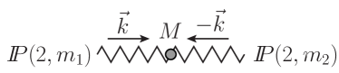
Figure 21: The fictitious reaction of two “real spin 2 pomerons” of momenta $\vec{k}$ and $-\vec{k}$ annihilating to a meson $M$.

We consider, thus, the annihilation of two “pomeron particles” of spin 2 and $z$-components of spin $m_{1}$ and $m_{2}$ giving a meson of spin $J$ and $z$-component $J_{z}$ in the c.m. system, that is, the rest system of $M$:

$$I\!\!P(\vec{k},2,m_{1})+I\!\!P(-\vec{k},2,m_{2})\to M(J,J_{z})\,,$$

$$m_{1,2}\in\{-2,\ldots,2\}\,,\quad J_{z}\in\{-J,\ldots,J\}\,.$$ (39)

Note that we use here the Wigner basis for all particles; see Wigner , and for instance, chapter 16.2 of Nachtmann90 , and Appendix C. Clearly, in (39) $M$ must have isospin and $G$ parity $I^{G}=0^{+}$ and charge conjugation $C=+1$. The question is: what are the possible values of spin $J$ and parity $P$ for meson $M$?

Let $a_{2,m}^{\dagger}(\vec{k})$, $a_{2,m}^{\dagger}(-\vec{k})$ be the creation operators for the “pomeron particles”. We can first construct the states of the two “pomerons” with definite orbital angular momentum $l$, $l_{z}$ and then those with given $l$, $l_{z}$ and total spin $S$, $S_{z}$. We get with $\hat{k}=\vec{k}/|\vec{k}|$, $Y_{l}^{l_{z}}(\hat{k})$ the spherical harmonics, and the usual Clebsch-Gordan coefficients

$$\left|2,m_{1};2,m_{2};l,l_{z}\right\rangle=\int d\Omega_{k}\,Y_{l}^{l_{z}}(\hat{k})\,a_{2,m_{1}}^{\dagger}(\vec{k})\,a_{2,m_{2}}^{\dagger}(-\vec{k})\left|0\right\rangle\,,$$ (40)

$$\left|S,S_{z};l,l_{z}\right\rangle=\sum_{m_{1},m_{2}}\left\langle 2,m_{1};2,m_{2}|S,S_{z}\right\rangle\left|2,m_{1};2,m_{2};l,l_{z}\right\rangle\,.$$ (41)

Here we have

$$l = 0,1,2,\ldots,$$

$$-l \leqslant l_{z}\leqslant l\,,$$

$$S = 0,1,2,3,4\,,$$

$$-S \leqslant S_{z}\leqslant S\,.$$ (42)

From Bose symmetry of our “pomeron particles” we find that

$$\left|S,S_{z};l,l_{z}\right\rangle=0\quad\mathrm{for}\;l-S\;\mathrm{odd}\,.$$ (43)

The parity transformation $U(P)$ gives

$$U(P)\left|S,S_{z};l,l_{z}\right\rangle=(-1)^{l}\left|S,S_{z};l,l_{z}\right\rangle\,.$$ (44)

It is straightforward to construct the two-pomeron states of definite total angular momentum $J$, $J_{z}$:

$$\left|l,S;J,J_{z}\right\rangle=\sum_{S_{z},l_{z}}\left\langle S,S_{z};l,l_{z}|J,J_{z}\right\rangle\left|S,S_{z};l,l_{z}\right\rangle\,.$$ (45)

Clearly, $J$ is then the spin of the produced meson in (39) and $P=(-1)^{l}$ its parity. In Table 6 we list the values of $J$ and $P$ of mesons which can be produced in our fictitious reaction (39) where we restrict ourselves to $l\leqslant 4$.

Table 6: The values, for orbital angular momentum $l$, of total spin $S$, total angular momentum $J$, and parity $P$, possible in the annihilation reaction (39). The continuation of the table for $l>4$ is straightforward.

$l$	$S$	$J$	$P$
0	0	0	$+$
	2	2
	4	4
1	1	0, 1, 2	$-$
	3	2, 3, 4
2	0	2	$+$
	2	0,1,2,3,4
	4	2,3,4,5,6
3	1	2,3,4	$-$
	3	0,1,2,3,4,5,6
4	0	4	$+$
	2	2,3,4,5,6
	4	0,1,2,3,4,5,6,7,8

It is clear that for each value of $l$, $S$, $J$, and $P$ listed in Table 6 we can construct a covariant Lagrangian density ${\cal L}^{\prime}$ coupling the field operator for the meson $M$ to the pomeron fields $I\!\!P_{\mu\nu}$. There, $l$ is related to the number of derivatives in ${\cal L}^{\prime}$, thus giving an indication of the angular momentum barrier in the production of $M$ in (39). In Table 7 we list interesting candidates for mesons $M$ in central production and the corresponding minimal values of $l$ and $S$ which can lead to the meson states according to Table 6.

Table 7: Candidates for mesons producible in pomeron-pomeron annihilation. The values of the minimal orbital angular momentum $l$ and of the corresponding total spin $S$ for the reactions (39) and (59) with tensorial ($I\!\!P_{T}$) and vectorial ($I\!\!P_{V}$) “pomeron particles”, respectively, are also indicated.

		$I\!\!P_{T}$		$I\!\!P_{V}$
$J^{PC}$	meson $M$	$l$	$S$	$l$	$S$
$0^{-+}$	$\eta$	1	1	1	1
	$\eta^{\prime}(958)$
$0^{++}$	$f_{0}(980)$	0	0	0	0
	$f_{0}(1370)$
	$f_{0}(1500)$
$1^{++}$	$f_{1}(1285)$	2	2	2	2
	$f_{1}(1420)$
$2^{++}$	$f_{2}(1270)$	0	2	0	2
	$f^{\prime}_{2}(1525)$
$4^{++}$	$f_{4}(2050)$	0	4	2	2

The strategy is now to construct for a given meson $M$ of Table 7 a coupling Lagrangian ${\cal L}_{I\!\!PI\!\!PM}^{\prime}$ corresponding to the $l$ and $S$ values listed there. We illustrate this here for the case of a $J^{PC}=0^{++}$ meson $M$. The case of a pseudoscalar meson $\tilde{M}$ is treated in Section II.2.

The Lagrangian ${\cal L}_{I\!\!PI\!\!PM}^{\prime}$ for a scalar meson ($J^{PC}=0^{++}$) corresponding to $l=S=0$ reads

$${\cal L}_{I\!\!PI\!\!PM}^{\prime}(x)=M_{0}\,g_{I\!\!PI\!\!PM}^{\prime}\,I\!\!P_{\mu\nu}(x)\,I\!\!P^{\mu\nu}(x)\,\chi(x)\,,$$ (46)

where $\chi(x)$ is the meson field operator, $M_{0}\equiv 1$ GeV, and $g_{I\!\!PI\!\!PM}^{\prime}$ is the dimensionless coupling constant. The “bare” vertex obtained from (46), see Fig. 22 (a),

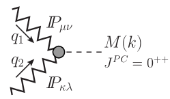
(a) (b)

Figure 22: A sketch of the pomeron-pomeron-scalar meson vertex for the tensorial (a) and vectorial (b) pomeron fusion.

reads

$$i\Gamma_{\mu\nu,\kappa\lambda}^{\prime(I\!\!PI\!\!P\to M)}\mid_{bare}=i\,g_{I\!\!PI\!\!PM}^{\prime}\,M_{0}\,\left(g_{\mu\kappa}g_{\nu\lambda}+g_{\mu\lambda}g_{\nu\kappa}-\frac{1}{2}g_{\mu\nu}g_{\kappa\lambda}\right)\,.$$ (47)

Here we have made the vertex traceless since the $I\!\!P_{\mu\nu}$ are supposed to have trace zero.

In Appendix C we use (47) to calculate the $T$-matrix element for the fictitious reaction (39) with a scalar meson. We show there that in the Wigner basis we get from (46) an amplitude containing values of $(l,S)$ = $(0,0)$, $(2,2)$, and $(4,4)$. But the higher terms are completely fixed by the lowest term $(l,S)=(0,0)$. This justifies to call the coupling (46) the one corresponding to $(l,S)=(0,0)$.

The coupling Lagrangian ${\cal L}_{I\!\!PI\!\!PM}^{\prime\prime}$ and vertex $\Gamma^{\prime\prime(I\!\!PI\!\!P\to M)}$ corresponding to $l=S=2$ read as follows:

$${\cal L}_{I\!\!PI\!\!PM}^{\prime\prime}(x)=\dfrac{1}{2M_{0}}\,g_{I\!\!PI\!\!PM}^{\prime\prime}\,\left[\partial^{\mu}I\!\!P^{\nu\rho}(x)-\partial^{\nu}I\!\!P^{\mu\rho}(x)\right]\,\left[\partial_{\mu}I\!\!P_{\nu\rho}(x)-\partial_{\nu}I\!\!P_{\mu\rho}(x)\right]\,\chi(x)\,,$$ (48)

$$i\Gamma_{\mu\nu,\kappa\lambda}^{\prime\prime(I\!\!PI\!\!P\to M)}(q_{1},q_{2})\mid_{bare}=\dfrac{i\,g_{I\!\!PI\!\!PM}^{\prime\prime}}{2M_{0}}$$

$$\times\left[q_{1\kappa}q_{2\mu}g_{\nu\lambda}+q_{1\kappa}q_{2\nu}g_{\mu\lambda}+q_{1\lambda}q_{2\mu}g_{\nu\kappa}+q_{1\lambda}q_{2\nu}g_{\mu\kappa}-2(q_{1}q_{2})(g_{\mu\kappa}g_{\nu\lambda}+g_{\nu\kappa}g_{\mu\lambda})\right]\,,$$ (49)

where $g_{I\!\!PI\!\!PM}^{\prime\prime}$ is the dimensionless coupling constant. The vertex (49) must be added coherently to the vertex (47).

In the production reaction (1) we cannot take the “bare” vertices ((47) and (49)) directly. We have to take into account that hadrons are extended objects, that is, we shall have to introduce form factors. The actual vertex which is assumed in this paper reads then as follows

$$i\Gamma_{\mu\nu,\kappa\lambda}^{(I\!\!PI\!\!P\to M)}(q_{1},q_{2})=\left(i\Gamma_{\mu\nu,\kappa\lambda}^{\prime(I\!\!PI\!\!P\to M)}\mid_{bare}+i\Gamma_{\mu\nu,\kappa\lambda}^{\prime\prime(I\!\!PI\!\!P\to M)}(q_{1},q_{2})\mid_{bare}\right)F_{I\!\!PI\!\!PM}(q_{1}^{2},q_{2}^{2})\,.$$ (50)

Unfortunately, the pomeron-pomeron-meson form factor is not well known as it is due to nonperturbative effects related to the internal structure of the respective meson. In practical calculations we take the factorized form with the following two approaches. Either we use

$$F^{M}_{I\!\!PI\!\!PM}(t_{1},t_{2})=F_{M}(t_{1})F_{M}(t_{2})\,,$$ (51)

with $F_{M}(t)$ the pion electromagnetic form factor in its simplest parametrization, valid for $t<0$,

$$F_{M}(t)=F_{\pi}(t)=\frac{1}{1-t/\Lambda_{0}^{2}}\,,$$ (52)

where $\Lambda_{0}^{2}=0.5$ GeV²; see e.g. (3.22) of DDLN . Alternatively, we use the exponential form given as

$$F^{E}_{I\!\!PI\!\!PM}(t_{1},t_{2})=\exp\left(\frac{t_{1}+t_{2}}{\Lambda_{E}^{2}}\right)\,,$$ (53)

where $\Lambda_{E}^{2}\approx 1$ GeV². This discussion of form factors applies also to the other pomeron-pomeron-meson vertices considered in this paper.

In the case of meson-exchange diagrams we use the monopole form factor which is normalized to unity at the on-shell point $t=m_{M}^{2}$

$$F(t)=\frac{\Lambda_{M}^{2}-m_{M}^{2}}{\Lambda_{M}^{2}-t}\,,$$ (54)

where $\Lambda_{M}>m_{M}$ and $t<0$. Alternatively, we use the exponential form

$$F(t)=\exp\left(\frac{t-m_{M}^{2}}{\Lambda_{E}^{2}}\right)\,.$$ (55)

The influence of the choice of the form-factor parameters is discussed in the results section.

Appendix B Vectorial pomeron

In this section we perform the same analysis for the vectorial pomeron ansatz as is done for the tensorial pomeron in Appendix A.

In the vectorial approach, see DDLN , DL , the pomeron is treated as a “$C=+1$ photon”. Its coupling to the proton reads

$$i\Gamma_{\mu}^{(I\!\!P_{V}pp)}(p^{\prime},p)=-i\,3\beta_{I\!\!PNN}\,F_{1}\bigl{(}(p^{\prime}-p)^{2}\bigr{)}\,M_{0}\,\gamma_{\mu}\,,$$ (56)

where $\beta_{I\!\!PNN}=1.87$ GeV^-1, $M_{0}\equiv 1$ GeV; compare to (30). The effective $I\!\!P_{V}$ propagator is given by

$$i\Delta_{\mu\nu}^{(I\!\!P_{V})}(s,t)=\frac{1}{M_{0}^{2}}\,g_{\mu\nu}\left(-is\alpha^{\prime}_{I\!\!P}\right)^{\alpha_{I\!\!P}(t)-1}\,,$$ (57)

with $\alpha_{I\!\!P}(t)$ and $\alpha^{\prime}_{I\!\!P}$ as in (33).

From (56) and (57) we get for proton-proton elastic scattering

$$\Braket{p(p_{1},\lambda_{1}),p(p_{2},\lambda_{2})}{{\cal T}}{p(p_{a},\lambda_{a}),p(p_{b},\lambda_{b})}\mid_{I\!\!P_{V}}\;\equiv$$

$${\cal M}^{2\to 2}_{\lambda_{a}\lambda_{b}\to\lambda_{1}\lambda_{2}}\mid_{I\!\!P_{V}}=(-i)\bar{u}(p_{1},\lambda_{1})i\Gamma_{\mu}^{(I\!\!P_{V}pp)}(p_{1},p_{a})u(p_{a},\lambda_{a})$$

$$\qquad\qquad\qquad\qquad\times i\Delta^{(I\!\!P_{V})\,\mu\nu}(s,t)$$

$$\qquad\qquad\qquad\qquad\times\bar{u}(p_{2},\lambda_{2})i\Gamma_{\nu}^{(I\!\!P_{V}pp)}(p_{2},p_{b})u(p_{b},\lambda_{b})$$

$$\qquad\qquad\qquad\xrightarrow{s\,\gg\,m_{p}^{2}}i\,2s\,\left[3\beta_{I\!\!PNN}\,F_{1}(t)\right]^{2}\,\left(-is\alpha^{\prime}_{I\!\!P}\right)^{\alpha_{I\!\!P}(t)-1}\,\delta_{\lambda_{1}\lambda_{a}}\,\delta_{\lambda_{2}\lambda_{b}}\,.$$ (58)

Comparing with (38) we see that for $s\gg m_{p}^{2}$, both, the tensorial and the vectorial pomeron give the same amplitude for $pp$ elastic scattering.

In the next step we consider the annihilation of two “vector-pomeron particles” into a meson $M$

$$I\!\!P_{V}(\vec{k},1,m_{1})+I\!\!P_{V}(-\vec{k},1,m_{2})\to M(J,J_{z})\,,$$

$$m_{1,2}\in\{-1,0,1\}\,,\quad J_{z}\in\{-J,\ldots,J\}\,;$$ (59)

compare to (39). Here, again, we use the Wigner basis. The same analysis as done after (39) for the tensorial pomeron can now be performed for the vectorial one. The result is given in Table 8 which is the analogue of Table 6 for the tensorial pomeron.

Table 8: The values of $l$, $S$, $J$, and $P$, of orbital angular momentum, total spin of the two “vector-pomeron particles”, total angular momentum, and parity of the state, respectively, possible in the vectorial pomeron annihilation reaction (59). We have $S\in\{0,1,2\}$, $P=(-1)^{l}$, $|l-S|\leqslant J\leqslant l+S$, and Bose symmetry requires $l-S$ to be even. The continuation of the table for $l>4$ is straightforward.

$l$	$S$	$J$	$P$
0	0	0	$+$
	2	2
1	1	0, 1, 2	$-$
2	0	2	$+$
	2	0,1,2,3,4
3	1	2,3,4	$-$
4	0	4	$+$
	2	2,3,4,5,6

As in Appendix A we illustrate the use of Table 8 by discussing the coupling of two vectorial pomerons to a $J^{PC}=0^{++}$ meson $M$. Let $\chi$ be the meson field, $I\!\!P_{V}^{\mu}$ the effective vector-pomeron field. The coupling corresponding to $(l,S)=(0,0)$ reads

$${\cal L^{\prime}}_{I\!\!P_{V}I\!\!P_{V}M}(x)=M_{0}\,g_{I\!\!P_{V}I\!\!P_{V}M}^{\prime}\,I\!\!P_{V\mu}(x)\,I\!\!P_{V}^{\mu}(x)\,\chi(x)\,$$ (60)

with $M_{0}\equiv 1$ GeV, and $g_{I\!\!P_{V}I\!\!P_{V}M}^{\prime}$ the dimensionless coupling constant. From (60) we get the “bare” vertex, see Fig. 22 (b),

$$i\Gamma_{\mu\nu}^{\prime(I\!\!P_{V}I\!\!P_{V}\to M)}\mid_{bare}=i\,g_{I\!\!P_{V}I\!\!P_{V}M}^{\prime}\,M_{0}\,2g_{\mu\nu}\,.$$ (61)

Using this vertex to calculate the amplitude for the fictitious reaction (59) we find, in the Wigner basis, contributions with $(l,S)=(0,0)$ and $(2,2)$ with the $(2,2)$ part completely fixed by the $(0,0)$ part; see Appendix C. Thus, we shall refer to the coupling (61) as the one corresponding to $(l,S)=(0,0)$.

For $l=S=2$ the coupling Lagrangian and vertex read as follows:

$${\cal L}_{I\!\!P_{V}I\!\!P_{V}M}^{\prime\prime}(x)=\dfrac{1}{2M_{0}}\,g_{I\!\!P_{V}I\!\!P_{V}M}^{\prime\prime}\,\left[\partial^{\mu}I\!\!P_{V}^{\nu}(x)-\partial^{\nu}I\!\!P_{V}^{\mu}(x)\right]\,\left[\partial_{\mu}I\!\!P_{V\nu}(x)-\partial_{\nu}I\!\!P_{V\mu}(x)\right]\,\chi(x)\,,$$ (62)

$$i\Gamma_{\mu\nu}^{\prime\prime(I\!\!P_{V}I\!\!P_{V}\to M)}(q_{1},q_{2})\mid_{bare}=\dfrac{2i\,g_{I\!\!P_{V}I\!\!P_{V}M}^{\prime\prime}}{M_{0}}\left[q_{2\mu}q_{1\nu}-(q_{1}q_{2})g_{\mu\nu}\right]\,,$$ (63)

where $g_{I\!\!P_{V}I\!\!P_{V}M}^{\prime\prime}$ is the dimensionless coupling constant.

The discussion of form factors for these vertices is identical to the one for the tensorial pomeron in Appendix A. Thus, for the full vertex for two vectorial pomerons giving a $0^{++}$ meson we add (61) and (63) and multiply the sum by a form factor

$$i\Gamma_{\mu\nu}^{(I\!\!P_{V}I\!\!P_{V}\to M)}(q_{1},q_{2})=\left(i\Gamma_{\mu\nu}^{\prime(I\!\!P_{V}I\!\!P_{V}\to M)}\mid_{bare}+i\Gamma_{\mu\nu}^{\prime\prime(I\!\!P_{V}I\!\!P_{V}\to M)}(q_{1},q_{2})\mid_{bare}\right)F_{I\!\!PI\!\!PM}(q_{1}^{2},q_{2}^{2}).$$ (64)

The coupling of two vectorial pomerons to a pseudoscalar mesons $\tilde{M}$ is given in Section II.2; cf. (14) and (15).

Appendix C Covariant $I\!\!PI\!\!PM$ couplings and the Wigner basis

In this appendix we discuss the relation of the covariant $I\!\!PI\!\!PM$ couplings to the classification of partial wave amplitudes in the Wigner basis as given in Table 6 for the tensorial and in Table 8 for the vectorial pomeron.

Let us consider as an example of the reaction (59) the annihilation of two fictitious “vectorial pomeron particles” of mass $m$ giving a $J^{PC}=0^{++}$ meson $M$:

$$I\!\!P_{V}(\vec{k},\vec{\varepsilon}_{1}^{\,W})+I\!\!P_{V}(-\vec{k},\vec{\varepsilon}_{2}^{\,W})\to M\,.$$ (65)

Here $\vec{\varepsilon}_{1,2}^{\,W}$ are the polarization vectors in the Wigner basis with

$$|\vec{\varepsilon}_{1}^{\,W}|=|\vec{\varepsilon}_{2}^{\,W}|=1\,.$$ (66)

To transform to the covariant polarization vectors $\varepsilon_{i}\,^{\mu}$ ($i=1,2$) we need the boost transformation $\Lambda_{\vec{k}}$:

$$(\Lambda_{\vec{k}}\,^{\mu}{}_{\;\;\nu})=\left(\begin{array}[]{cl}\dfrac{k^{0}}{m}&\;\,\dfrac{k^{j}}{m}\\ \\ \dfrac{k^{i}}{m}&\;\,\delta^{ij}+\hat{k}^{i}\hat{k}^{j}\Bigl{(}\dfrac{k^{0}}{m}-1\Bigr{)}\\ \end{array}\right)\,,$$ (70)

$$i,j\in\left\{1,2,3\right\},\quad\hat{k}=\vec{k}/|\vec{k}|\,.$$ (71)

We have

$$(\varepsilon_{1}\,^{\mu})=\Lambda_{\vec{k}}\left(\begin{array}[]{c}0\\ \vec{\varepsilon}_{1}^{\,W}\\ \end{array}\right)\,,$$ (74)

$$(\varepsilon_{2}\,^{\mu})=\Lambda_{-\vec{k}}\left(\begin{array}[]{c}0\\ \vec{\varepsilon}_{2}^{\,W}\\ \end{array}\right)\,.$$ (77)

From the vertex (61) we get the amplitude for reaction (65) as follows

$$\Braket{M}{{\cal T}}{I\!\!P_{V}(\vec{k},\vec{\varepsilon}_{1}^{\,W}),I\!\!P_{V}(-\vec{k},\vec{\varepsilon}_{2}^{\,W})}=\Gamma_{\mu\nu}^{\prime(I\!\!P_{V}I\!\!P_{V}\to M)}\varepsilon_{1}\,^{\mu}\varepsilon_{2}\,^{\nu}=-2\,M_{0}\,g_{I\!\!P_{V}I\!\!P_{V}M}^{\prime}$$

$$\times\Bigl{[}\Bigl{(}1+\frac{2}{3}\frac{\vec{k}^{2}}{m^{2}}\Bigr{)}\vec{\varepsilon}_{1}^{\,W}\cdot\vec{\varepsilon}_{2}^{\,W}+\frac{1}{m^{2}}\Bigl{(}k^{i}k^{j}-\frac{1}{3}\delta^{ij}\vec{k}^{2}\Bigr{)}\Bigl{(}\varepsilon_{1}^{W\,i}\varepsilon_{2}^{W\,j}+\varepsilon_{2}^{W\,i}\varepsilon_{1}^{W\,j}-\frac{2}{3}\delta^{ij}\vec{\varepsilon}_{1}^{\,W}\cdot\vec{\varepsilon}_{2}^{\,W}\Bigr{)}\Bigr{]}.\,\,\,\,\,\,\,\,$$ (78)

From the vertex (63) we get

$$\Braket{M}{{\cal T}}{I\!\!P_{V}(\vec{k},\vec{\varepsilon}_{1}^{\,W}),I\!\!P_{V}(-\vec{k},\vec{\varepsilon}_{2}^{\,W})}=\frac{2g_{I\!\!P_{V}I\!\!P_{V}M}^{\prime\prime}}{M_{0}}\Bigl{[}\Bigl{(}k_{2}\varepsilon_{1}\Bigr{)}\Bigl{(}k_{1}\varepsilon_{2}\Bigr{)}-\Bigl{(}k_{1}k_{2}\Bigr{)}\Bigl{(}\varepsilon_{1}\varepsilon_{2}\Bigr{)}\Bigr{]}=\frac{2g_{I\!\!P_{V}I\!\!P_{V}M}^{\prime\prime}}{M_{0}}$$

$$\times\Bigl{[}\Bigl{(}\frac{4}{3}\vec{k}^{2}+m^{2}\Bigr{)}\vec{\varepsilon}_{1}^{\,W}\cdot\vec{\varepsilon}_{2}^{\,W}-\Bigl{(}k^{i}k^{j}-\frac{1}{3}\delta^{ij}\vec{k}^{2}\Bigr{)}\Bigl{(}\varepsilon_{1}^{W\,i}\varepsilon_{2}^{W\,j}+\varepsilon_{2}^{W\,i}\varepsilon_{1}^{W\,j}-\frac{2}{3}\delta^{ij}\vec{\varepsilon}_{1}^{\,W}\cdot\vec{\varepsilon}_{2}^{\,W}\Bigr{)}\Bigr{]}.$$ (79)

Thus, in the Wigner basis we get from both vertices, (61) and (63), partial wave amplitudes with $(l,S)=(0,0)$ and $(2,2)$. Multiplying the vertices (61) and (63) with suitable form factors and forming linear combinations of them it would be possible to construct vertices giving only $(l,S)=(0,0)$ or $(2,2)$ in the Wigner basis. But this would be a very cumbersome procedure. Therefore, we shall in this paper stick to the simple vertices as given above and label (61) with $(l,S)=(0,0)$ and (63) with $(l,S)=(2,2)$ since (61) has no momenta and (63) two momenta. But we have keep in mind that the translation of the power of momenta in the covariant vertices to the angular momentum $l$ in the Wigner basis is not one to one.

For the tensorial pomeron the situation is similar. We discuss the reaction (39) for a scalar meson $M$

$$I\!\!P(\vec{k},\varepsilon_{1}^{W\,ij})+I\!\!P(-\vec{k},\varepsilon_{2}^{W\,hl})\to M\,,$$

$$i,j,h,l\in\left\{1,2,3\right\}\,.$$ (80)

Here $\varepsilon_{1,2}^{W\,ij}$ are the polarization tensors of the fictitious “tensor-pomeron particle” of mass $m$ in the Wigner basis. We have:

$$\varepsilon_{1}^{W\,ij}=\varepsilon_{1}^{W\,ji},\quad\varepsilon_{2}^{W\,ij}=\varepsilon_{2}^{W\,ji},$$

$$\varepsilon_{1}^{W\,ij}\delta_{ij}=\varepsilon_{2}^{W\,ij}\delta_{ij}=0\,,$$

$$(\varepsilon_{1}^{W\,ij})^{*}(\varepsilon_{1}^{W\,ji})=1,\quad(\varepsilon_{2}^{W\,ij})^{*}(\varepsilon_{2}^{W\,ji})=1\,.$$ (81)

The covariant polarization tensors are

$$\varepsilon_{1}\,^{\mu\nu}=\Lambda_{\vec{k}}\,^{\mu}{}_{\;\;i}\,\Lambda_{\vec{k}}\,^{\nu}{}_{\;\;j}\,\varepsilon_{1}^{W\,ij}\,,$$

$$\varepsilon_{2}\,^{\mu\nu}=\Lambda_{-\vec{k}}\,^{\mu}{}_{\;\;i}\,\Lambda_{-\vec{k}}\,^{\nu}{}_{\;\;j}\,\varepsilon_{2}^{W\,ij}\,.$$ (82)

With (82) we obtain the amplitude for (80) from the vertex (47) as follows:

$$\Braket{M}{{\cal T}}{I\!\!P(\vec{k},\varepsilon_{1}^{W\,ij}),I\!\!P(-\vec{k},\varepsilon_{2}^{W\,hl})}=2\,M_{0}\,g_{I\!\!PI\!\!PM}^{\prime}\,\varepsilon_{1}\,^{\mu\nu}\varepsilon_{2}\,{}_{\mu\nu}\,.$$ (83)

Inserting here the explicit expressions from (82) we see easily that the amplitude (83) has, in the Wigner basis, partial wave parts with $(l,S)=(0,0),(2,2)$, and $(4,4)$. Similarly, also the vertex (49) gives contributions with $(l,S)=(0,0),(2,2)$, and $(4,4)$. We label the vertex (47) with $(l,S)=(0,0)$ since it has no momenta, and (49) with $(l,S)=(2,2)$ since it is quadratic in the momenta.

The discussion of other pomeron-pomeron-meson couplings when going from the covariant forms to the partial wave amplitudes in the Wigner basis can be done in a completely analogous way.

Appendix D Kinematic relations and the high-energy small-angle limit

The following relations hold, cf. (2),

$$s_{13} = (p_{a}+q_{2})^{2}$$

$$= (s-2m_{p}^{2})\,\xi_{2}+m_{p}^{2}+t_{2}\,,$$

$$s_{23} = (p_{b}+q_{1})^{2}$$ (84)

$$= (s-2m_{p}^{2})\,\xi_{1}+m_{p}^{2}+t_{1}\,,$$

where $\xi_{1}=\dfrac{p_{b}\cdot q_{1}}{p_{b}\cdot p_{a}}$ and $\xi_{2}=\dfrac{p_{a}\cdot q_{2}}{p_{a}\cdot p_{b}}$ are the fractional energy losses of the protons with momenta $p_{a}$ and $p_{b}$, respectively. We consider now the reaction (1) in the overall c.m. system with the $z$ axis along $\vec{p}_{a}$. We have then

$$p_{a}=\left(\begin{array}[]{c}p_{a}^{0}\\ 0\\ 0\\ |\vec{p}_{a}|\\ \end{array}\right),\quad p_{b}=\left(\begin{array}[]{c}p_{b}^{0}\\ 0\\ 0\\ -|\vec{p}_{b}|\\ \end{array}\right),$$ (93)

$$p_{a}^{0}=p_{b}^{0}=\frac{\sqrt{s}}{2},\quad|\vec{p}_{a}|=|\vec{p}_{b}|=\frac{1}{2}\sqrt{s-4m_{p}^{2}}\,.$$ (94)

With $i=1,2$ we get

$$p_{i}=\left(\begin{array}[]{c}p_{i}^{0}\\ \vec{p}_{i\perp}\\ p_{iz}\\ \end{array}\right),\quad q_{i}=\left(\begin{array}[]{c}q_{i}^{0}\\ \vec{q}_{i\perp}\\ q_{iz}\\ \end{array}\right),$$ (101)

$$\vec{p}_{i\perp}=|\vec{p}_{i\perp}|\left(\begin{array}[]{c}\cos\phi_{i}\\ \sin\phi_{i}\\ \end{array}\right),\quad\vec{q}_{i\perp}=-\vec{p}_{i\perp}\,.$$ (104)

The azimuthal angle $\phi_{pp}$ between the two outgoing protons in (1) is given by

$$\phi_{pp}=\phi_{1}-\phi_{2}\,.$$ (105)

The “glueball variable” CK97 $dP_{\perp}=|d\vec{P}_{\perp}|$ is defined by the difference of the transverse momentum vectors

$$d\vec{P}_{\perp}=\vec{q}_{1\perp}-\vec{q}_{2\perp}=\vec{p}_{2\perp}-\vec{p}_{1\perp}\,.$$ (106)

Further relations are as follows (no summation over $i$ in (108) for $\xi_{i}t_{i}$)

$$m_{M}^{2}=k^{2}=2q_{1}q_{2}+t_{1}+t_{2}$$

$$\quad=\frac{(s-2m_{p}^{2})^{3}}{s(s-4m_{p}^{2})}\xi_{1}\xi_{2}+t_{1}+t_{2}-2\vec{q}_{1\perp}\cdot\vec{q}_{2\perp}+\frac{(s-2m_{p}^{2})}{s(s-4m_{p}^{2})}\left[t_{1}t_{2}-2m_{p}^{2}(t_{1}\xi_{2}+t_{2}\xi_{1})\right],$$ (107)

$$t_{i}=-\vec{q}_{i\perp}^{\,2}+\frac{1}{s(s-4m_{p}^{2})}\left[(s-2m_{p}^{2})^{2}(\xi_{i}t_{i}-\xi_{i}^{2}m_{p}^{2})-t_{i}^{2}m_{p}^{2}\right],$$ (108)

$$p_{i}^{0}=\frac{\sqrt{s}}{2}(1-\xi_{i})+\frac{1}{2\sqrt{s}}(2m_{p}^{2}\xi_{i}-t_{i})\,,$$ (109)

$$\varepsilon_{\mu_{1}\mu_{2}\rho\sigma}(p_{1}+p_{a})^{\mu_{1}}(p_{2}+p_{b})^{\mu_{2}}(q_{1}-q_{2})^{\rho}(q_{1}+q_{2})^{\sigma}=-8\sqrt{s}\,\vec{p}_{a}\cdot(\vec{p}_{1\perp}\times\vec{p}_{2\perp})$$

$$\qquad\qquad\qquad\qquad\qquad\qquad\qquad\qquad\qquad\quad\quad\;\;\,=8\sqrt{s}\,|\vec{p}_{a}||\vec{p}_{1\perp}||\vec{p}_{2\perp}|\sin\phi_{pp}\,.$$ (110)

In Figs. 10 and 20 we have shown distributions in rapidity, $\mathrm{y}_{M}$, and pseudorapidity, $\eta_{M}$, of the produced meson $M$ in the overall c.m. system. We discuss here their kinematic relation. We have with

$$k=\left(\begin{array}[]{c}k^{0}\\ \vec{k}_{\perp}\\ k_{z}\\ \end{array}\right)\,,$$ (114)

the four-momentum of meson $M$ ($k^{2}=m_{M}^{2}$),

$$\mathrm{y}_{M} = \frac{1}{2}\,\ln\frac{k^{0}+k_{z}}{k^{0}-k_{z}}=\ln\frac{\sqrt{k_{z}^{2}+\vec{k}^{2}_{\perp}+m_{M}^{2}}+k_{z}}{\sqrt{\vec{k}^{2}_{\perp}+m_{M}^{2}}}\,,$$ (115)

$$\eta_{M} = \frac{1}{2}\,\ln\frac{|\vec{k}|+k_{z}}{|\vec{k}|-k_{z}}=\ln\frac{\sqrt{k_{z}^{2}+\vec{k}^{2}_{\perp}}+k_{z}}{\sqrt{\vec{k}^{2}_{\perp}}}\,.$$ (116)

Consider now the distributions of meson $M$ in ($\mathrm{y}_{M},\vec{k}^{2}_{\perp}$) and ($\eta_{M},\vec{k}^{2}_{\perp}$). We have

$$f(\mathrm{y}_{M},\vec{k}^{2}_{\perp})d\mathrm{y}_{M}d(\vec{k}^{2}_{\perp})=\tilde{f}(\eta_{M},\vec{k}^{2}_{\perp})d\eta_{M}d(\vec{k}^{2}_{\perp})\,,$$ (117)

$$\tilde{f}(\eta_{M},\vec{k}^{2}_{\perp})=f(\mathrm{y}_{M},\vec{k}^{2}_{\perp})\frac{\partial\mathrm{y}_{M}/\partial k_{z}}{\partial\eta_{M}/\partial k_{z}}\mid_{\vec{k}^{2}_{\perp}\;\mathrm{fixed}}\,,$$ (118)

where

$$\frac{\partial\mathrm{y}_{M}/\partial k_{z}}{\partial\eta_{M}/\partial k_{z}}\mid_{\vec{k}^{2}_{\perp}\;\mathrm{fixed}}=\frac{\sqrt{k_{z}^{2}+\vec{k}^{2}_{\perp}}}{\sqrt{k_{z}^{2}+\vec{k}^{2}_{\perp}+m_{M}^{2}}}\equiv w(k_{z},\vec{k}^{2}_{\perp})\,.$$ (119)

Clearly, for large $|\mathrm{y}_{M}|$ and correspondingly large $|\eta_{M}|$ we have $|k_{z}|\gg m_{M}$ and the transformation factor $w(k_{z},\vec{k}^{2}_{\perp})\to 1$. On the other hand, for $|\mathrm{y}_{M}|\to 0$ corresponding to $|\eta_{M}|\to 0$ and $k_{z}\to 0$ we have $w(0,\vec{k}^{2}_{\perp})<1$. Thus, we conclude that, for fixed $\vec{k}^{2}_{\perp}\neq 0$ a $\mathrm{y}_{M}$ distribution which is roughly constant for $|\mathrm{y}_{M}|\to 0$ will give a dip in the $\eta_{M}$ distribution for $|\eta_{M}|\to 0$. A dip in the $\mathrm{y}_{M}$ distribution for $|\mathrm{y}_{M}|\to 0$ will be deepened in the $\eta_{M}$ distribution. To get the $\mathrm{y}_{M}$ and $\eta_{M}$ distributions of Figs. 10 and 20 we still have to integrate in (117) over $\vec{k}^{2}_{\perp}$. We note, however, that integration over $\vec{k}^{2}_{\perp}$ at fixed $\mathrm{y}_{M}$ is, in general, not the same as integration at fixed $\eta_{M}$. Nevertheless, if the unintegrated distributions of (117) in $(\mathrm{y}_{M},\vec{k}^{2}_{\perp})$, respectively $(\eta_{M},\vec{k}^{2}_{\perp})$, behave “reasonably” we should be able to replace in the above arguments fixed $\vec{k}^{2}_{\perp}$ by some mean value $\langle\vec{k}^{2}_{\perp}\rangle$. Then the above features will survive. That is, a $\mathrm{y}_{M}$ distribution being roughly constant for $|\mathrm{y}_{M}|\to 0$ will give a dip for $|\eta_{M}|\to 0$, as observed in Fig. 10. A dip in the $\mathrm{y}_{M}$ distribution for $|\mathrm{y}_{M}|\to 0$ will be deepened in the $\eta_{M}$ distribution, as observed in Fig. 20.

We consider now the high-energy small-angle limit where we require in reaction (1)

$$|t_{1}|,|t_{2}|\ll m_{p}^{2}\,,\quad m_{M}^{2}\ll s\,,\quad\xi_{1},\xi_{2}=\mathcal{O}(m_{M}/\sqrt{s})\,.$$ (120)

In this limit we have the simple relations

$$\xi_{1}\cong\frac{s_{23}}{s}\,,\quad\xi_{2}\cong\frac{s_{13}}{s}\,,\quad m_{M}^{2}\cong s\xi_{1}\xi_{2}=\frac{s_{13}s_{23}}{s}\,,\quad t_{1}\cong-\vec{q}_{1\perp}^{\,2}\,,\quad t_{2}\cong-\vec{q}_{2\perp}^{\,2}\,;$$ (121)

$$\bar{u}(p_{1},\lambda_{1})\gamma^{\mu}u(p_{a},\lambda_{a})\cong(p_{1}+p_{a})^{\mu}\delta_{\lambda_{1}\lambda_{a}}\,,$$

$$\bar{u}(p_{2},\lambda_{2})\gamma^{\mu}u(p_{b},\lambda_{b})\cong(p_{2}+p_{b})^{\mu}\delta_{\lambda_{2}\lambda_{b}}\,;$$ (122)

$$(p_{1}+p_{a},p_{2}+p_{b})\cong 2s\,;$$ (123)

$$(q_{1},p_{2}+p_{b})(q_{2},p_{1}+p_{a})-(q_{1},q_{2})(p_{1}+p_{a},p_{2}+p_{b})\cong 2s\,\vec{p}_{1\perp}\cdot\vec{p}_{2\perp}=2s\,|\vec{p}_{1\perp}||\vec{p}_{2\perp}|\cos\phi_{pp}\,.$$

(124)

We see from (120) and (121) that in this limit both subenergies squared become large

$$s_{13},s_{23}=\mathcal{O}(m_{M}\sqrt{s})\,.$$ (125)

References

- (1) A. Donnachie, H.G. Dosch, P.V. Landshoff and O. Nachtmann, Pomeron Physics and QCD, Cambridge University Press, Cambridge, U.K. 2002.
- (2) J.R. Forshaw and D.A. Ross, Quantum Chromodynamics and the Pomeron, Cambrigde University Press, Cambridge, U.K. 1997.
-
(3)
F.E. Close and G.A. Schuler, Phys. Lett. B464 (1999) 279;
F.E. Close and G.A. Schuler, Phys. Lett. B458 (1999) 127;
F.E. Close A. Kirk and G.A. Schuler, Phys. Lett. B477 (2000) 13. - (4) O. Nachtmann, a talk: A model for high-energy soft reactions, at ECT* workshop on exclusive and diffractive processes in high energy proton-proton and nucleus-nucleus collisions, Trento, February 27 - March 2, 2012.
- (5) C. Ewerz, M. Maniatis and O. Nachtmann, arXiv:1309.3478 [hep-ph].
- (6) R. Pasechnik, A. Szczurek and O. Teryaev, Phys. Rev.D83 (2011) 074017.
- (7) P. Lebiedowicz, R. Pasechnik and A. Szczurek, Phys. Lett. B701 (2011) 434.
- (8) R. Maciuła, R. Pasechnik and A. Szczurek, Phys. Rev. D83 (2011) 114034.
- (9) P. Lebiedowicz, R. Pasechnik and A. Szczurek, Nucl. Phys. B867 (2013) 61.
- (10) P. Lebiedowicz and A. Szczurek, Phys. Rev. D81 (2010) 036003.
-
(11)
L.A. Harland-Lang, V.A. Khoze, M.G. Ryskin and W.J. Stirling, Eur. Phys. J. C71 (2011) 1545;
L.A. Harland-Lang, V.A. Khoze, M.G. Ryskin and W.J. Stirling, Eur. Phys. J. C72 (2012) 2110. - (12) P. Lebiedowicz and A. Szczurek, Phys. Rev. D85 (2012) 014026.
- (13) T. Arens, O. Nachtmann, M. Diehl and P.V. Landshoff, Z. Phys. C74 (1997) 651.
- (14) A.B. Kaidalov, V.A. Khoze, A.D. Martin, and M.G. Ryskin, Eur. Phys. J. C31 (2003) 387.
- (15) V.A. Petrov, R.A. Ryutin, A.E. Sobol, and J.-P. Guillaud, JHEP 007 (2005) 0506.
- (16) J. Ellis and D. Kharzeev, Preprint CERN-TH/98-349, arXiv:9811222 [hep-ph].
- (17) N.I. Kochelev, arXiv:9902203 [hep-ph].
- (18) D. Kharzeev and E. Levin, Phys. Rev. D63 (2001) 073004.
- (19) E. Shuryak and I. Zahed, Phys. Rev. D68 (2003) 034001.
- (20) WA102 Collaboration (D. Barberis et al.), Phys. Lett. B397 (1997) 339.
- (21) WA102 Collaboration (D. Barberis et al.), Phys. Lett. B427 (1998) 398.
- (22) WA102 Collaboration (D. Barberis et al.), Phys. Lett. B462 (1999) 462.
- (23) WA102 Collaboration (D. Barberis et al.), Phys. Lett. B467 (1999) 165.
- (24) WA102 Collaboration (D. Barberis et al.), Phys. Lett. B474 (2000) 423.
- (25) A. Kirk, Phys. Lett. B489 (2000) 29.
- (26) S. Weinberg, The Quantum Theory of Fields, Vol. II, Cambridge University Press, Cambridge, U.K. 1996.
- (27) N.I. Kochelev, T. Morii and A.V. Vinnikov, Phys. Lett. B457 (1999) 202.
-
(28)
A. Donnachie and P.V. Landshoff, Nucl. Phys. B231 (1984) 189;
A. Donnachie and P.V. Landshoff, Nucl. Phys. B244 (1984) 322;
A. Donnachie and P.V. Landshoff, Nucl. Phys. B267 (1986) 690;
A. Donnachie and P.V. Landshoff, Phys. Lett. B191 (1987) 309;
A. Donnachie and P.V. Landshoff, Phys. Lett. B185 (1987) 403;
P.V. Landshoff and O. Nachtmann, Z. Phys. C35 (1987) 405;
A. Donnachie and P.V. Landshoff, Nucl. Phys. B303 (1988) 634. - (29) L.P. Kaptari and B. Kämpfer, Eur. Phys. J. A37 (2008) 69.
- (30) K. Nakayama, Y. Oh and H. Haberzettl, Jour. Korean Phys. Soc. 59 (2011) 224.
- (31) K. Nakayama and H. Haberzettl, Phys. Rev. C69 (2004) 065212.
- (32) K. Nakayama, J. Speth and T.-S. H. Lee, Phys. Rev. C65 (2002) 045210.
- (33) WA91 Collaboration (D. Barberis et al.), Phys. Lett. B388 (1996) 853.
- (34) F.E. Close and A. Kirk, Phys. Lett. B397 (1997) 333.
- (35) WA76 Collaboration (T.A. Armstrong et al.), Z. Phys. C51 (1991) 351.
- (36) A. Cisek, P. Lebiedowicz, W. Schäfer, and A. Szczurek, Phys. Rev. D83 (2011) 114004.
- (37) A. Szczurek and P. Lebiedowicz, Nucl. Phys. A826 (2009) 101.
- (38) C. Di Donato, G. Ricciardi and I. Bigi, Phys. Rev. D85 (2012) 013016.
- (39) P. Kroll and K. Passek-Kumericki, Phys. Rev. D67 (2003) 054017.
- (40) F.E. Close and A. Kirk, Phys. Lett. B489 (2000) 24.
- (41) N.I. Kochelev, T. Morii, B.L. Reznik and A.V. Vinnikov, Eur. Phys. J. A8 (2000) 405.
-
(42)
P. Lebiedowicz and A. Szczurek, Phys. Rev. D87 (2013) 074037;
P. Lebiedowicz and A. Szczurek, Phys. Rev. D87 (2013) 114013. - (43) Particle Data Group (J. Beringer et al.), Phys. Rev. D86 (2012) 010001.
- (44) P. Castoldi, R. Escribano and J. M. Frere, Phys. Lett. B425 (1998) 359.
- (45) A. Szczurek, R.S. Pasechnik and O.V. Teryaev, Phys. Rev. D75 (2007) 054021.
- (46) W. Kilian and O. Nachtmann, Eur. Phys. J. C5 (1998) 317.
-
(47)
F. Nerling, for the COMPASS Collaboration, EPJ Web Conf. 37 (2012) 01016;
A. Austregesilo and T. Schlüter, for the COMPASS Collaboration, PoS QNP2012 (2012) 098. - (48) J. Turnau, for the STAR Collaboration, EPJ Web Conf. 37 (2012) 06010.
-
(49)
M.G. Albrow, A. Świȩch and M. Żurek, EPJ Web Conf. 37 (2012) 06011;
M.G. Albrow et al., AIP Conf. Proc. 1523 (2012) 294. - (50) R. Schicker, for the ALICE Collaboration, arXiv:1205.2588 [hep-ex].
- (51) R. Staszewski, P. Lebiedowicz, M. Trzebiński, J. Chwastowski and A. Szczurek, Acta Phys. Polon. B42 (2011) 1861.
- (52) E.P. Wigner, Ann. Math. 40 (1939) 149.
- (53) O. Nachtmann, Elementary Particle Physics, Springer-Verlag, Berlin, Heidelberg 1990.