Freely-moving observer in (quasi) anti de Sitter space

Abstract

A quantum scalar field in anti de Sitter space is considered in two coordinate systems: static and FRW-like ones. It is shown that quantum vacua corresponding to each of these coordinatizations are not unitary equivalent. A choice of a physical ground state between these vacua is discussed under different setups.

I Introduction

Historically, Minkowski spacetime is a manifold wherein a quantization of a field was first performed. The Poincaré-invariant no-particle state is known as Minkowski vacuum that is associated with inertial observers. 40 years ago it was discovered that a quantum vacuum defined by a uniformly accelerated observer is not unitary equivalent to Minkowski one Fulling . Moreover, Minkowski vacuum for such an observer is seen as a thermal bath of particles defined with respect to the observer’s reference frame. This phenomenon is known as Davies-Unruh effect Davies ; Unruh ; Birrell&Davies ; Mukhanov&Winitzki ; Crispino&Higuchi&Matsas . Later it was also shown that the notion of a particle of a massive field in Milne spacetime is inequivalent to the Minkowski particle, where Milne vacuum has been defined as a no-particle state that becomes the conformal vacuum in the massless limit Sommerfield . If the conformal quantum field occupies Milne vacuum, then a radiation with a Planck spectrum and negative energy density is present in it Birrell&Davies .

Another example of a manifold where similar situation takes place is de Sitter space. De Sitter hyperboloid is a curved maximally symmetric spacetime with a negative, constant curvature $R=-12H_{\text{dS}}^{2}$. It can be covered entirely or partially by various coordinate systems Mukhanov ; Griffiths&Podolsky . Quantization of a field performed in different coordinatizations generally leads to a definition of different quantum vacua. In particular, a comoving observer in dS defines its own no-particle state $|0_{\text{S}}\rangle$ that is associated with the static coordinate frame, where the observer is at its origin. The Unruh-DeWitt detector moving along a time-like geodesic in the de Sitter hyperboloid will be excited like it is in the thermal bath with the Hawking-Gibbons temperature $T_{\text{HG}}=H_{\text{dS}}/2\pi$ Gibbons&Hawking . Thus, the vacuum state associated with the field quantized in static dS is not unitary equivalent to the closed one, i.e. $|0_{\text{S}}\rangle\nsim|0_{\text{CT}}\rangle$, where $|0_{\text{CT}}\rangle$ is the Chernikov-Tagirov ground state, as well as to the flat vacuum Birrell&Davies .

In the present paper we shall consider anti de Sitter hyperboloid that is also a curved maximally symmetric manifold, but with a positive, constant curvature. There are known variety of coordinate patches which parameterize the whole or some set of the AdS hyperboloid points Griffiths&Podolsky . We shall take into our consideration two of them, namely static (or global) and open (or FRW-like with the negative spatial curvature, see Griffiths&Podolsky ) coordinates. Static coordinates cover the entire AdS, whereas open coordinates embrace merely half of it. Therefore one may a priori await that quantization performed in each coordinate systems leads to inequivalent quantum vacua. Thus, the aim of our research is to uncover how open vacuum $|0_{\text{O}}\rangle$ is related with static one $|0_{\text{S}}\rangle$ (both defined below) as well as to figure out whether a freely-moving detector in AdS will be somehow excited.

In Section II, a real scalar field model is considered in four-dimensional AdS. For the sake of avoiding unnecessary complications, we assume that it is invariant under the conformal symmetry. The question of a physical vacuum state is examined by analysing cosmological consequences resulting from taking into account quantum corrections at one-loop approximation in semiclassical Einstein equation for each of them.

In Section III, a two-dimensional massive scalar field is studied. In this case, we shall further investigate the vacua under different setups as well as compare them with the Minkowski state.

We work throughout in units implying $\hbar=c=k_{\text{B}}=G=1$. The signature of the metric tensor is $(+,-,-,-)$ and $R_{\mu\nu}=\partial_{\lambda}\Gamma_{\mu\nu}^{\lambda}-\partial_{\nu}\Gamma_{\mu\lambda}^{\lambda}+\Gamma_{\rho\lambda}^{\lambda}\Gamma_{\mu\nu}^{\rho}-\Gamma_{\rho\mu}^{\lambda}\Gamma_{\lambda\nu}^{\rho}$.

II Conformal scalar field in AdS₄

Anti de Sitter spacetime can be represented as a four dimensional hyperboloid

$$x_{0}^{2}-x_{1}^{2}-x_{2}^{2}-x_{3}^{2}+x_{4}^{2} = H^{-2}$$ (1)

embedded in $\mathbf{R}^{5}$ with the line element $ds^{2}=dx_{0}^{2}-dx_{1}^{2}-dx_{2}^{2}-dx_{3}^{3}+dx_{4}^{2}$ Hawking&Ellis .

Anti de Sitter space is not globally hyperbolic. Its topology is given by $\mathbf{S}\times\mathbf{R}^{3}$, where the circle $\mathbf{S}$ corresponds to time coordinate. This means it contains closed time-like curves. A standard approach for avoiding casual paradoxes in AdS is to unwrap $\mathbf{S}$ and to consider its universal covering $\mathbf{R}$ Hawking&Ellis . In the following, we deal with universal covering space only. Besides, Cauchy surface is absent in it. The quantization procedure is performed by imposing certain boundary conditions at spatial time-like infinity which ensure, in particular, the energy conservation Avis&Isham&Storey ; Breitenlohner&Freedman .

As has been above mentioned, we shall deal with static and open coordinates (see App. A). Static coordinates cover the entire hyperboloid and, as a consequence, one needs to impose the boundary conditions on the field to have a well-defined quantum theory Avis&Isham&Storey ; Breitenlohner&Freedman . Open coordinates cover merely a part of the hyperboloid that is globally hyperbolic.

Static AdS₄

The mode expansions of the quantum scalar field conformally coupled with gravity in static coordinates read

$$\hat{\phi}(x) = \sum\limits_{nlm}\left\{\begin{array}[]{l}\hat{a}_{nlm}^{\phantom{}}u_{nlm}^{\phantom{\dagger}}(x)+\hat{a}_{nlm}^{\dagger}u_{nlm}^{*}(x)\,,\\[7.11317pt] \hat{b}_{nlm}^{\phantom{}}v_{nlm}^{\phantom{\dagger}}(x)+\hat{b}_{nlm}^{\dagger}v_{nlm}^{*}(x)\,,\end{array}\right.$$ (4)

where star denotes the complex conjugation. The positive-frequency modes $u_{nlm}(x)$ and $v_{nlm}(x)$ with respect to the time translation operator are

$$u_{nlm}(x) = A_{nl}\,e^{-i(2n+2+l)\eta}\,Y_{lm}(\theta,\varphi)(\sin\chi)^{l}\cos\chi\,C_{2n+1}^{l+1}(\cos\chi)\,,$$ (5a)

$$v_{nlm}(x) = B_{nl}\,e^{-i(2n+1+l)\eta}\,Y_{lm}(\theta,\varphi)(\sin\chi)^{l}\cos\chi\,C_{2n}^{l+1}(\cos\chi)\,,$$ (5b)

where $n,l\in\mathbb{N}_{0}$ and $m\in\{-l,...,+l\}$, $A_{nl}$ and $B_{nl}$ are normalization coefficients Avis&Isham&Storey ; Breitenlohner&Freedman . The static vacuum $|0_{\text{S}}\rangle=|0_{\text{S}_{1}}\rangle\otimes|0_{\text{S}_{2}}\rangle$ is annihilated by both $\hat{a}_{nlm}$ and $\hat{b}_{nlm}$: $\hat{a}_{nlm}|0_{\text{S}_{1}}\rangle=\hat{b}_{nlm}|0_{\text{S}_{2}}\rangle=0$. The Fock space of particle states is built by cyclic operations of the creation operators $\hat{a}_{nlm}^{\dagger}$ and $\hat{b}_{nlm}^{\dagger}$ on $|0_{\text{S}}\rangle$.

Open AdS₄

The mode expansion of the field in open coordinates is given by

$$\hat{\phi}(\bar{x}) = \sum\limits_{lm}\int\limits_{0}^{+\infty}d\omega\Big{(}\hat{c}_{\omega lm}^{\phantom{\dagger}}w_{\omega lm}^{\phantom{\dagger}}(\bar{x})+\hat{c}_{\omega lm}^{\dagger}w_{\omega lm}^{*}(\bar{x})\Big{)}\,,$$ (6)

where the mode functions $w_{\omega lm}(\bar{x})$ regular at $\bar{\chi}=0$ are

$$w_{\omega lm}(\bar{x}) = \frac{C_{\omega l}}{a(\bar{\eta})}\,e^{-i\omega\bar{\eta}}\,Y_{lm}(\bar{\theta},\bar{\phi})\left(\sinh\bar{\chi}\right)^{-\frac{1}{2}}P_{i\omega-1/2}^{-l-1/2}(\cosh\bar{\chi})\,,$$ (7)

where $C_{\omega l}$ is a real normalization coefficient Sasaki&Tanaka&Yamamoto . Open vacuum $|0_{\text{O}}\rangle$ is defined as being annihilated by $\hat{c}_{\omega lm}$. The Fock space is generated by acting by the creation operator $\hat{c}_{\omega lm}^{\dagger}$ on this vacuum.

In contrast to the static case, there is no time-like Killing vector in open AdS that can be used to define the Hamiltonian operator being the representation of the time translation on space of quantum states. However, the conformal time-like Killing vector $K=\partial_{\bar{\eta}}$ allows us to introduce

$$\hat{H} = \int d\Sigma_{\mu}\hat{T}^{\mu}_{\nu}K^{\nu}\;\;=\;\;\frac{1}{2}\sum\int d\omega\omega\Big{(}\hat{c}_{\omega lm}^{\dagger}\hat{c}_{\omega lm}^{\phantom{\dagger}}+\hat{c}_{\omega lm}^{\phantom{\dagger}}\hat{c}_{\omega lm}^{\dagger}\Big{)}\,,$$ (8)

where $T_{\mu\nu}$ is the energy-momentum tensor of the field. The operator $\hat{H}$ is conserved due to the conformal symmetry. It can be interpreted as a generator of the time translation acting on the rescaled field $\hat{\phi}_{\text{r}}(\bar{x})\equiv a(\bar{\eta})\hat{\phi}(\bar{x})$, i.e. $\mathcal{L}_{K}\hat{\phi}_{\text{r}}=i\big{[}\hat{H},\hat{\phi}_{\text{r}}\big{]}$, where $\mathcal{L}_{K}$ is the Lie derivative along $K$. Thus, the rescaled modes (7) are positive frequency modes with respect to $\partial_{\bar{\eta}}$ and $|0_{\text{O}}\rangle$ is called the conformal vacuum Birrell&Davies .

Although the conformal time $\bar{\eta}$ lies on the whole real line $\mathbf{R}$, the expansion (6) of the quantum field is performed in terms of the physical time $\bar{t}$ only for $(0,\pi/H)$ that corresponds to the upper wedge depicted in Fig. 1. However, the same expansion can be used for the lower wedge, wherein $\bar{t}\in(-\pi/H,0)$. Shortly, a difference between these wedges will be discussed. The modes in the rest of the wedges can be straightforwardly obtained from the upper and lower ones.

II.1 Bogolyubov transformation

A curve $\chi=0$ and $\Delta\theta=\Delta\phi=0$ is a geodesic in static AdS. An observer that moves along it will detect nothing, provided the quantum field is in $|0_{\text{S}_{a}}\rangle$, where $a\in\{1,2\}$. Indeed, the response function $\mathcal{F}(E)$ of the Unruh-DeWitt detector with respect to $|0_{\text{S}_{a}}\rangle$ is

$$\mathcal{F}(E) \propto \int\limits_{-\infty}^{+\infty}d\Delta\tau\,e^{-iE\Delta\tau}\,\left(\frac{1}{\sin^{2}\left(\frac{1}{2}H\Delta\tau-i\varepsilon\right)}-\frac{(-1)^{a}}{\cos^{2}\left(\frac{1}{2}H\Delta\tau-i\varepsilon\right)}\right)\,,\quad\varepsilon\rightarrow+0\,,$$ (9)

where $E$ is an eigenstate of detector’s Hamiltonian, $\tau$ the proper time along observer’s geodesic Birrell&Davies . Representing the integrand as a series (1.422.2 and 1.422.4 in Gradshteyn&Ryzhik ) and regarding it as a contour one over a closed contour in an infinite semicircle in a lower-half $\Delta\tau$ plane, one obtains $\mathcal{F}(E)=0$ that proves the statement.

A curve $\Delta\bar{\chi}=0$ and $\Delta\theta=\Delta\phi=0$ represents a comoving geodesic in open AdS. These geodesics belong to a time-like set of integral curves of the vector $\xi=\sin\eta\cos\chi\,\partial_{\eta}+\cos\eta\sin\chi\,\partial_{\chi}$. This vector field is time-like in open AdS, but is future-directed for $\eta\in(2\pi k,\pi+2\pi k)$ and past-directed for $\eta\in(-\pi+2\pi k,2\pi k)$, where $k\in\mathbb{N}$. Outside of open AdS the vector field $\xi$ is space-like and null on the horizons $\eta=\pm\chi+\pi k$. The vacuum state invariant under $\exp(-i\hat{H}\bar{\eta})$ is the conformal one, i.e. $|0_{\text{O}}\rangle$. Since for any comoving observer a relation between the conformal time $\bar{\eta}$ and the proper one $\tau$ does not depend on spatial coordinates, the Unruh-DeWitt detector will be similarly exited or unexcited for any of them.

At the points $\chi=\bar{\chi}=0$ and $\theta,\phi=\text{const}$, two vacua are defined. As has been shown above, the detector moving along this geodesic will remain unexcited if the field in $|0_{\text{S}_{a}}\rangle$. However, this detector may response if the field is in $|0_{\text{O}}\rangle$. In order to find how these vacua are related to each other, we perform the Bogolyubov transformation that represents the annihilation $\hat{c}_{\omega lm}^{\phantom{}}$ and creation $\hat{c}_{\omega lm}^{\dagger}$ operators defining conformal vacuum $|0_{\text{O}}\rangle$ as a linear combinations of analogous operators associated with $|0_{\text{S}_{a}}\rangle$. Note, there is no inverse Bogolyubov transformation, because open coordinates do not cover the entire hyperboloid.

This canonical, unitary map is completely determined by the Bogolyubov coefficients

$$\begin{array}[]{lcl}\alpha_{\omega lm,nl^{\prime}m^{\prime}}&=&\big{(}u_{nl^{\prime}m^{\prime}}(x),w_{\omega lm}(\bar{x})\big{)}\,,\\[7.11317pt] \beta_{\omega lm,nl^{\prime}m^{\prime}}&=&\big{(}u_{nl^{\prime}m^{\prime}}^{*}(x),w_{\omega lm}(\bar{x})\big{)}\,,\end{array}$$ (10)

where the round brackets denote the Klein-Gordon scalar product Birrell&Davies . We have used in (10) an expansion of the quantum field expressed through $u$-modes for the sake of concreteness. The same result can be shown is valid for the expansion through $v$-modes. Below we discuss the upper wedge. At the end of this subsection we shall point out which changes must be made to accommodate (10) with the lower wedge.

Calculation of the coefficients is considerably simplified if one takes a hypersurface of equal-time events $\Sigma$ specified by $\bar{\eta}=0$. Having chosen it, one obtains

$$\begin{array}[]{lcl}\alpha_{\omega lm,nl^{\prime}m^{\prime}}&=&N_{ln}(\omega)\,\delta_{ll^{\prime}}\,\delta_{mm^{\prime}}\,M_{n,l}^{+}(\omega)\,,\\[7.11317pt] \beta_{\omega lm,nl^{\prime}m^{\prime}}&=&N_{ln}(\omega)\,\delta_{ll^{\prime}}\,\delta_{mm^{\prime}}\,M_{n,l}^{-}(\omega)\,,\end{array}$$ (11)

where $N_{nl}(\omega)$ is written down in App. D and

$$M_{n,l}^{\pm}(\omega) \equiv \int\limits_{0}^{+\infty}d\bar{\chi}\,\left(\omega\pm\frac{2+l+2n}{\cosh\bar{\chi}}\right)\frac{(\sinh\bar{\chi})^{l+\frac{3}{2}}}{(\cosh\bar{\chi})^{l+2}}\,\big{(}\tanh\left(\bar{\chi}/2\right)\big{)}^{l+\frac{1}{2}}$$

$$\times {}_{2}F_{1}\left(-n,n+l+2;\frac{3}{2};\frac{1}{\cosh^{2}(\bar{\chi})}\right){}_{2}F_{1}\left(\frac{1}{2}-i\omega,\frac{1}{2}+i\omega;l+\frac{3}{2};-\sinh^{2}\left(\bar{\chi}/2\right)\right)\,,$$

where the Gegenbauer $C_{\nu}^{\mu}(z)$ and the associated Legendre $P_{\nu}^{\mu}(z)$ functions have been rewritten via the hypergeometric one ${}_{2}F_{1}(\alpha,\beta;\gamma;z)$ Gradshteyn&Ryzhik .

The integrals (II.1) for $l=0$ can be exactly evaluated and are

$$M_{n,0}^{\pm} = \mp\frac{\pi^{2}\exp\left(\pm\frac{\pi\omega}{2}\right)}{\sqrt{2}\sinh^{2}(\pi\omega)}\,\frac{{}_{2}F_{1}\left(-2-2n,i\omega;i\omega-1-2n;-1\right)}{\Gamma\left(2n+3\right)\Gamma\left(1-i\omega\right)\Gamma\left(i\omega-1-2n\right)}\,,$$ (13)

where $J_{n}^{\pm}(\omega)$ and $I_{n}^{\pm}(\omega)$ given in App. B have been used. Thus, we obtain

$$\alpha_{\omega 00,n00} = -e^{\pi\omega}\beta_{\omega 00,n00}\,.$$ (14)

For arbitrary $l\geq 0$, one can express $M_{n,l+1}^{\pm}$ through $M_{n,l}^{\pm}$ and $M_{n+1,l}^{\pm}$ as follows

$$M_{n,l+1}^{\pm} = \frac{2l+3}{4\big{(}\omega^{2}+(l+1)^{2}\big{)}}\Big{(}(3+2l+2n)M_{n,l}^{\pm}-(2n+3)M_{n+1,l}^{\pm}\Big{)}\,$$ (15)

(see App. C for details). Consequently, one has

$$\alpha_{\omega lm,n^{\prime}l^{\prime}m^{\prime}} = -e^{\pi\omega}\beta_{\omega lm,n^{\prime}l^{\prime}m^{\prime}}\,.$$ (16)

Repeating the same kind of calculations for the Bogolyubov coefficients in the lower wedge, one finds that they are equal to (11) multiplied by $(-1)^{n+1}$, where $n$ is odd for $u$-modes, and even for $v$-modes.

II.2 Relation between static $|0_{\text{S}}\rangle$ and open $|0_{\text{O}}\rangle$ vacua

Vacua $|0_{\text{S}_{a}}\rangle$ and $|0_{\text{O}}\rangle$ are not unitary equivalent. Despite of their orthogonality, no-particle state $|0_{\text{O}}\rangle$ can formally be represented as a state realized by infinite number of particles defined with respect to $|0_{\text{S}_{a}}\rangle$. In order to see this, one has to represent the annihilation operator $\hat{c}_{\omega lm}$ as follows

$$\hat{c}_{\omega lm}^{\phantom{}} = \cosh\theta_{\omega}\,\hat{d}_{\omega lm}^{\phantom{}}-\sinh\theta_{\omega}\,\hat{f}_{\omega lm}^{\dagger}\,,$$ (17)

where by definition

$$\hat{d}_{\omega lm}^{\phantom{}} \equiv \frac{1}{\cosh\theta_{\omega}}\,\sum\limits_{n^{\prime}l^{\prime}m^{\prime}}\alpha_{\omega lm,nl^{\prime}m^{\prime}}\hat{a}_{n^{\prime}l^{\prime}m^{\prime}}\,,\quad\hat{f}_{\omega lm}^{\phantom{}}\;\;\equiv\;\;\frac{-1}{\sinh\theta_{\omega}^{*}}\,\sum\limits_{n^{\prime}l^{\prime}m^{\prime}}\beta_{\omega lm,nl^{\prime}m^{\prime}}^{*}\hat{a}_{n^{\prime}l^{\prime}m^{\prime}}\,.$$ (18)

It is shown in App. D that if one takes $\tanh\theta_{\omega}=e^{-\pi\omega}$, then

$$\big{[}\hat{d}_{\omega lm}^{\phantom{}},\hat{d}_{\omega^{\prime}l^{\prime}m^{\prime}}^{\dagger}\big{]} = \big{[}\hat{f}_{\omega lm}^{\phantom{}},\hat{f}_{\omega^{\prime}l^{\prime}m^{\prime}}^{\dagger}\big{]}\;\;=\;\;\delta(\omega-\omega^{\prime})\,\delta_{ll^{\prime}}\,\delta_{mm^{\prime}}\,,$$ (19a)

$$\big{[}\hat{d}_{\omega lm}^{\phantom{}},\hat{f}_{\omega^{\prime}l^{\prime}m^{\prime}}^{\phantom{}}\big{]} = \big{[}\hat{d}_{\omega lm}^{\phantom{}},\hat{f}_{\omega^{\prime}l^{\prime}m^{\prime}}^{\dagger}\big{]}\;\;=\;\;0$$ (19b)

hold. Such a pair of operators can be used to obtain

$$|0_{\text{O}}\rangle = Z^{-1}\exp\left(\sum\int d\omega e^{-\pi\omega}\hat{d}_{\omega lm}^{\dagger}\hat{f}_{\omega lm}^{\dagger}\right)|0_{\text{S}_{1}}\rangle\,,\quad\ln(Z)\;=\;\frac{\pi}{24}\delta(0)\sum(2l+1)\,,$$ (20)

where summations are implied over the discrete indices Umezawa . Both operators $\hat{d}_{\omega lm}$ and $\hat{f}_{\omega lm}$ annihilate static vacuum $|0_{\text{S}_{1}}\rangle$. Since $\hat{d}_{\omega lm}|0_{\text{O}}\rangle=e^{-\pi\omega}\hat{f}_{\omega lm}^{\dagger}|0_{\text{O}}\rangle$ and $\hat{f}_{\omega lm}|0_{\text{O}}\rangle=e^{-\pi\omega}\hat{d}_{\omega lm}^{\dagger}|0_{\text{O}}\rangle$, one has

$$\langle 0_{\text{O}}|\hat{d}_{\omega lm}^{\dagger}\hat{d}_{\omega^{\prime}l^{\prime}m^{\prime}}^{\phantom{}}|0_{\text{O}}\rangle = \frac{1}{e^{2\pi\omega}-1}\,\delta(\omega-\omega^{\prime})\delta_{ll^{\prime}}\delta_{mm^{\prime}}$$ (21)

and the same for the $f$-operators. The equation (21) implies that the conformal vacuum $|0_{\text{O}}\rangle$ can be regarded as a thermal bath of particles created by applying $\hat{d}_{\omega lm}^{\dagger}$ on $|0_{\text{S}_{1}}\rangle$.

The operators (18) are not independent: $\hat{f}_{\omega lm}=i(-1)^{l}\,\hat{d}_{-\omega lm}$. There must be a unitary equivalent quantization of the field in static AdS, such that the rescaled field is expanded through modes which are eigenfunctions of the vector field $\xi$. The creation operator must be given then by $\hat{d}_{plm}^{\dagger}$, whereas $p\in\mathbf{R}$ and $\omega=|p|$. Except for the fact that vector $\xi$ is not one of the generators of the anti de Sitter group $\text{SO}(3,2)$, this resembles an equivalent quantization in Minkowski space, wherein the field can also be expanded through modes being eigenfunctions of the Lorentz operator Crispino&Higuchi&Matsas .

Thus, a freely-moving detector will be thermally excited, provided the quantum field is in the conformal vacuum. Expressing $\omega$ via the physical frequency, i.e. $\omega_{\text{ph}}=\omega/a(\bar{t})$, one obtains that the temperature ascribed to the thermal condensate is equal to $T_{\text{AdS}}=(2\pi a(\bar{t}))^{-1}$, where $a(\bar{t})=H^{-1}\cos(H\bar{t})$. At this point, we merely note that $T_{\text{AdS}}$ diverges when $\cos(H\bar{t})=0$. Below we shall discuss a physical consequence of this result.

II.3 Choice of physical vacuum

In order to address a question of physicality of the vacua, we shall compute the renormalized energy-momentum tensor of the field in each of them, because the quantum field under consideration reveals itself physically through gravity. For instance, the renormalized stress tensor for the conformal scalar field in static vacuum in dS diverges at the event horizon, while it is finite and proportional to the metric for closed as well as flat vacua Candelas&Dowker2902 . Thus, the physical vacuum occupied by the quantum field in de Sitter space corresponds to Chernikov-Tagirov state Sciama&Candelas&Deutsch .

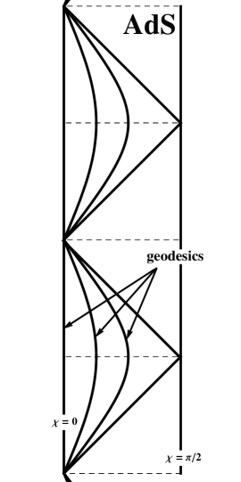
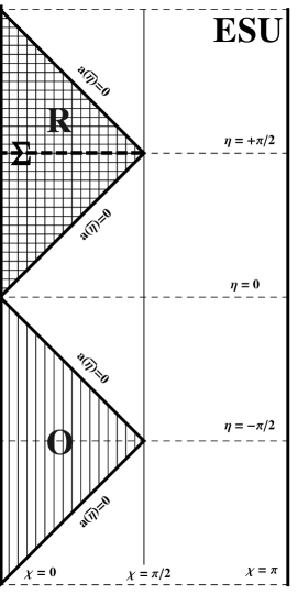
Figure 1: Left: conformal diagram of Anti de Sitter space. Right: conformal diagram of Einstein static universe (ESU) with embedded open AdS (O wedges filled by vertical lines) and Rindler (R wedge filled by horizontal lines) spaces in it.

The Euclidean section of entire AdS₄ is the hyperbolic space H⁴. The $\zeta$-function regularization method has been applied in H⁴ to derive the exact form of the one-loop effective action Camporesi&Higuchi . In this approach, the renormalized stress tensor corresponds to $|0_{\text{S}_{1}}\rangle$, as it follows from the comparison of two-point correlation functions calculated by $\zeta$-function method and directly summing the modes Burgess&Luetken . Thus, one has

$$\langle\hat{T}_{\nu}^{\mu}\rangle_{\text{S}_{1}} = \frac{H^{4}}{960\pi^{2}}\,\delta_{\nu}^{\mu}\,,$$ (22)

where $\langle...\rangle_{\text{S}_{1}}$ denotes the vacuum expectation value with respect to $|0_{\text{S}_{1}}\rangle$, i.e. $\langle 0_{\text{S}_{1}}|...|0_{\text{S}_{1}}\rangle$.

This result can be obtained in a different way. The Feynman two-point function $G_{\text{F}}^{1}(x,y)$ corresponding to $|0_{\text{S}_{1}}\rangle$ satisfies the scalar field equation with two $\delta$-sources which are located at $y$ and its antipodal point $y_{\text{A}}=-y$ Avis&Isham&Storey . The effective action is

$$W[\,g_{\mu\nu}] = -\frac{i}{2}\ln\det\big{(}-\hat{G}_{\text{F}}(1+\hat{\pi})\big{)}\,,$$ (23)

where $\langle x|\hat{G}_{\text{F}}|y\rangle=G_{\text{F}}(x,y)$ satisfies the field equation with the standard $\delta$-source and $\hat{\pi}$ is the inversion operator: $\hat{\pi}|x\rangle=|-x\rangle$ Birrell&Davies ; DeWitt . Since the determinant of a matrix product equals the product of their determinants, one can get rid of $\ln\det(1+\hat{\pi})$ by an infinite shift of the effective action $W[\,g_{\mu\nu}]$ that does not depend on the metric and, hence, has no physical consequences. Then, following the ordinary procedure, the trace anomaly can be derived that gives (22). Hence, one obtains

$$\langle\hat{T}_{\nu}^{\mu}\rangle_{\text{S}_{2}} = \frac{H^{4}}{960\pi^{2}}\,\delta_{\nu}^{\mu}\,.$$ (24)

This derivation may be supported by the following independent result derived by the point-splitting method: the renormalized stress tensor of a conformal scalar field that inhabits in half Einstein static universe (topologically $\mathbf{R}\times\mathbf{S}^{3}$) and satisfies Dirichlet or Neumann boundary conditions at the equator of the sphere $\mathbf{S}^{3}$ is exactly equal to the stress tensor of the field if it would be defined on entire $\mathbf{S}^{3}$ Kennedy&Unwin .

To compute $\langle\hat{T}_{\nu}^{\mu}\rangle_{\text{O}}$, one needs to take into account that wedges of open AdS can be conformally mapped into Rindler spacetime (see Fig. 1). Thus, one has

$$\langle\hat{T}_{\nu}^{\mu}\rangle_{\text{O}} = \frac{H^{4}}{960\pi^{2}}\,\delta_{\nu}^{\mu}-\frac{1}{480\pi^{2}a^{4}(\bar{\eta})}\left(\delta_{\nu}^{\mu}-\frac{4}{3}\,\delta_{i}^{\mu}\,\delta_{i\nu}\right)\,,$$ (25)

where summation with respect to $i$ running from 1 to 3 is implied Candelas&Dowker2902 .

The result (25) can be also derived by the point-splitting method supplemented by the symmetry properties of the problem. The anomalous trace specifies the renormalized stress tensor of a conformal scalar field in conformally flat space up to the local, conserved, traceless tensor (denoted as ${}^{(4)}H_{\mu\nu}$ in Birrell&Davies ). This non-geometric part of $\langle\hat{T}_{\nu}^{\mu}\rangle_{\text{O}}$ is unambiguously fixed, if the renormalized stress tensor of the field in open static universe $\langle\hat{T}_{\nu}^{\mu}\rangle_{\text{OSU}}$ is known. The point-splitting approach gives $\langle\hat{T}_{\nu}^{\mu}\rangle_{\text{OSU}}=0$ Bunch . Taking then into account the isometries of the metric and the continuity equation, i.e. $\nabla_{\mu}\langle\hat{T}_{\nu}^{\mu}\rangle_{\text{O}}=0$, one deduces (25).

The second term on the right-hand side of (25) represents a radiation with a negative energy density that vanishes in the classical limit: $\hbar\rightarrow 0$. It is worth noticing that the same situation occurs in Milne universe, wherein a comoving observer registers a thermal radiation with the negative energy density, provided the quantum field is in the conformal Milne vacuum Birrell&Davies .

The renormalized stress tensor with respect to static vacuum $\langle\hat{T}_{\nu}^{\mu}\rangle_{\text{S}_{a}}$ behaves itself equally well throughout the space, while $\langle\hat{T}_{\nu}^{\mu}\rangle_{\text{O}}$ diverges at the horizons, where $a(\bar{\eta})$ vanishes. It will be shown in the next subsection that AdS in open coordinates is unstable if the field occupies $|0_{\text{O}}\rangle$.

II.4 Backreaction

The Einstein equation with the quantum correction reads

$$R_{\mu\nu}-\frac{1}{2}\,g_{\mu\nu}R = \Lambda g_{\mu\nu}-\gamma_{2}\hbar\Big{(}RR_{\mu\nu}+g_{\mu\nu}\Box R-R_{;\mu\nu}-\frac{1}{4}\,g_{\mu\nu}R^{2}\Big{)}-\frac{\gamma_{3}\hbar}{a^{4}(\bar{\eta})}\left(g_{\mu\nu}-\frac{4}{3}\,g_{i\mu}\,\delta_{i\nu}\right)$$ (26)

$$-\gamma_{1}\hbar\left(\frac{2}{3}\,RR_{\mu\nu}-R_{\mu\lambda}R_{\nu}^{\lambda}-\frac{1}{4}\,g_{\mu\nu}R^{2}+\frac{1}{2}\,g_{\mu\nu}R_{\lambda\rho}R^{\lambda\rho}\right)+\text{O}(\hbar^{2})\,,$$

where $\langle\hat{T}_{\mu\nu}\rangle_{\text{O}}$ has been already substituted, $\gamma_{1}\equiv 1/360\pi$, $\gamma_{2}$ is a finite coefficient depending on the mass scale $\mu$, and $\gamma_{3}\equiv 1/60\pi$.

Using the order reduction method for throwing away spurious solutions Parker&Simon , one obtains the following first order nonlinear equation

$$3(a^{\prime})^{2}-3a^{2} = \Lambda a^{4}\left(1+\frac{\Lambda}{3}\,\gamma_{1}\hbar\right)-\gamma_{3}\hbar+\text{O}(\hbar^{2})\,.$$ (27)

where prime stands for the differentiation over the conformal time $\bar{\eta}$. It is solved up to the second order of $\hbar$ by

$$a(\bar{\eta}) = \frac{1}{\widetilde{H}\cosh(\bar{\eta})}+\frac{\gamma_{3}\hbar}{12}\sqrt{\frac{-\Lambda}{3}}\left(\cosh(\bar{\eta})+3\,\frac{\bar{\eta}\sinh(\bar{\eta})-\cosh(\bar{\eta})}{\cosh^{2}(\bar{\eta})}\right)+\text{O}(\hbar^{2})\,,$$ (28)

where $3\widetilde{H}^{2}=-\Lambda(1+\gamma_{1}\hbar\Lambda/3)$, an integration constant has been fixed by the condition: $a(0)=1/\widetilde{H}+\text{O}(\hbar)$, and a solution corresponding to the shift in time has been omitted.

From the equation (28) one immediately sees that there exists $\bar{\eta}_{0}>0$, such that for $|\bar{\eta}|>\bar{\eta}_{0}$ the correction of order $\hbar$ in $a(\bar{\eta})$ starts to dominate. It means that anti de Sitter space with the quantum field being in $|0_{\text{O}}\rangle$ is unstable, provided it has been somehow realized.

If the field is in $|0_{\text{S}}\rangle$, then the quantum corrections merely lead to a tiny decrease of the curvature.

III Massive scalar field in AdS₂

Two-dimensional anti de Sitter space can be obtained from (1) by setting $x_{2}=x_{3}=0$. The metric tensor in static or open coordinates are obtained by taking $\theta=0$ and $\phi=\text{const}$ in (41) or (44), where $\chi\in(-\frac{\pi}{2},+\frac{\pi}{2})$ and $\bar{\chi}\in\mathbf{R}$, respectively.

Static AdS₂

The massive quantum scalar field can be expanded as

$$\hat{\phi}(x) = \sum\limits_{n=0}^{+\infty}\left\{\begin{array}[]{l}u_{n}^{\phantom{\dagger}}(x)\hat{a}_{n}^{\phantom{}}+u_{n}^{*}(x)\hat{a}_{n}^{\dagger}\,,\\[7.11317pt] v_{n}^{\phantom{\dagger}}(x)\hat{b}_{n}^{\phantom{}}+v_{n}^{*}(x)\hat{b}_{n}^{\dagger}\,.\end{array}\right.$$ (31)

where the positive-frequency modes with respect to the translation operator along time coordinate are given by

$$u_{n}(x) = A_{n}\,e^{-i(2n+1+\lambda)\eta}\,(\cos\chi)^{\lambda}\,C_{2n+1}^{\lambda}(\sin\chi)\,,$$ (32a)

$$v_{n}(x) = B_{n}\,e^{-i(2n+\lambda)\eta}\,(\cos\chi)^{\lambda}\,C_{2n}^{\lambda}(\sin\chi)\,,$$ (32b)

$\lambda^{2}-\lambda=2\xi_{\text{R}}+(m/H)^{2}$ and $\lambda>1/2$, where $\xi_{\text{R}}$ is the coupling constant of the field with the scalar curvature, $A_{n}$ and $B_{n}$ are real normalization coefficients. The energy flux through the spatial boundary of anti de Sitter space vanishes for both sets of modes, thus the energy of the field is conserved. In addition, the scalar product is preserved as well Sakai&Tanii . The static vacuum is defined as a state being annihilated by both $\hat{a}_{n}$ and $\hat{b}_{n}$ for any $n\in\mathbb{N}_{0}$.

Open AdS₂

The metric tensor in open coordinates is homogeneous, therefore the field can be expanded through the eigenfunctions of the translation operator along the spatial coordinate

$$\hat{\phi}(\bar{x}) = \int\limits_{-\infty}^{+\infty}dp\Big{(}w_{p}(\bar{x})\,\hat{c}_{p}^{\phantom{}}+w_{p}^{*}(\bar{x})\,\hat{c}_{p}^{\dagger}\Big{)}\,,$$ (33)

where $w_{p}(\bar{x})=\varphi_{p}(\bar{\eta})\,e^{ip\bar{\chi}}$. The function $\varphi_{k}(\bar{\eta})$ satisfies

$$\Big{(}\partial_{\bar{\eta}}^{2}+p^{2}+a^{2}(\bar{\eta})\big{[}m^{2}+\xi_{\text{R}}R(\bar{\eta})\big{]}\Big{)}\varphi_{p}(\bar{\eta}) = 0\,,$$ (34)

where $R(\bar{\eta})$ is the Ricci scalar.

The general solution of (34) with $a(\bar{\eta})=(H\cosh\bar{\eta})^{-1}$ can be written in terms of Legendre Q-functions Gradshteyn&Ryzhik in the following form

$$\varphi_{p}(\bar{\eta}) = C_{p}(\cosh\bar{\eta})^{\frac{1}{2}}\Big{(}Q_{\nu}^{\mu}(i\sinh\bar{\eta})+\gamma_{p}Q_{-\nu-1}^{\mu}(i\sinh\bar{\eta})\Big{)}\,,$$ (35)

where $\nu=i\omega-\frac{1}{2}$, $\omega=|p|$, $\mu=\lambda-\frac{1}{2}$, $C_{p}$ and $\gamma_{p}$ are integration constants. The associated Legendre functions are defined in the complex plane except on $(-\infty,1)$. In particular, it implies the discontinuity Gradshteyn&Ryzhik : $Q_{\nu}^{\mu}(+i0)\neq Q_{\nu}^{\mu}(-i0)$. Therefore, we take the solution (35) for $\bar{\eta}>0$ and perform analytical continuation on negative time: $Q_{\nu}^{\mu}(i\sinh\bar{\eta})\rightarrow e^{i\pi\mu}(Q_{\nu}^{\mu}(i\sinh\bar{\eta})-i\pi P_{\nu}^{\mu}(i\sinh\bar{\eta}))$, where $\bar{\eta}<0$ on the right-hand side.

III.1 Bogolyubov transformation

The choice of $\gamma_{p}$ determines no-particle state in open coordinates. To compare them with static vacuum, one needs to compute the Bogolyubov coefficients. In order to simplify calculations, one may choose a surface $\bar{\eta}=+0$. The same result must be obtained in the case $\bar{\eta}=-0$ after performing the analytic continuation. In both cases we do get the same result

$$\frac{\beta_{pn}}{\alpha_{pn}} = \mp\frac{(1+\gamma_{p})e^{-2\pi i\lambda}}{\gamma_{p}e^{-\pi\omega}+e^{\pi\omega}}\,,$$ (36)

where the minus sign is taken for $u$-modes and the plus sign is for $v$-modes.

According to (36), the modes (35) with $\gamma_{p}=-1$ corresponds to static vacuum. Thus, a comoving observer in open AdS will see no particles along his movement in this case.

In the limits $\bar{\eta}\rightarrow\pm\infty$, the scale factor vanishes and $a^{\prime}/a\rightarrow\mp 1$. The zeroth-order approximation of the WKB-type solution Birrell&Davies gives

$$\varphi_{p}(\bar{\eta}) \sim e^{-i\omega\bar{\eta}}\,,\quad\bar{\eta}\;\;\rightarrow\;\;\pm\infty\,.$$ (37)

The next order gives a vanishing contribution at past and future time infinities. The exact solution will coincide with the approximate WKB solution in remote past if one chooses $\gamma_{p}=-e^{\pi\omega}\sin(\pi\lambda)\csc(\pi(\lambda+i\omega))$. Unless $\lambda$ is a positive integer, out-vacuum is filled by particles defined with respect to in-vacuum. However, such vacuum would be unphysical, because it implies a discontinuity in a density number of particles in the points between the wedges. For $\lambda\in\mathbb{N}$, in-vacuum and out-vacuum coincide and equal to the conformal one at the conformal time infinities. Plugging $\gamma_{p}=0$ into (36), one finds $|\beta_{pn}/\alpha_{pn}|=e^{-\pi\omega}$. Thus, if the field occupies this vacuum, then a freely-moving observer will register a thermal bath.

III.2 Relation between $|0_{\text{S}}\rangle$ and Minkowski vacuum $|0_{\text{M}}\rangle$

One can show that for open vacuum just defined the renormalized stress tensor $\langle T_{\nu}^{\mu}\rangle_{\text{O}}$ diverges at the horizons as it does in the four-dimensional case.

Assume $\lambda=1$, i.e. the conformal invariant case, and the scale factor behaves itself with the conformal time according to

$$a(\bar{\eta}) = a_{0}+\frac{1}{H\cosh\bar{\eta}}\,,\quad a_{0}=\text{const}>0\,.$$ (38)

The universe becomes Minkowski spacetime at past and future time infinities and anti de Sitter spacetime for $a_{0}H\cosh\bar{\eta}\ll 1$. At remote past it is natural to define Minkowski vacuum, such that $\phi_{p}(\bar{\eta})\sim e^{-i\omega\bar{\eta}}$, where $\omega=|p|$ as before. The AdS modes which correspond to the positive-frequency modes in Minkowski space at $\bar{\eta}\rightarrow\pm\infty$ are specified by setting $\gamma_{p}=0$ in (35). Thus, a geodesic observer that starts his journey from Minkowski spacetime will detect a thermal bath of particles at the AdS stage of the universe evolution. Note that the renormalized stress tensor vanishes at past and future infinities.

IV Concluding remarks

A quantization of the conformal scalar field in four-dimensional AdS in static and open coordinates leads to a definition of inequivalent quantum vacua. The former is associated with a freely-moving observer being located at the origin. The latter is a conformal vacuum associated with open coordinate system that resembles FRW-like universe with the negative spatial curvature and the scale factor periodically expanding from and contracting to the zero value: $a(\bar{t})=H^{-1}\cos(H\bar{t})$. Under the assumption that the quantum field occupies the conformal vacuum, $|0_{\text{O}}\rangle$, it has been shown that a geodesically moving observer will register a thermal bath of particles. The temperature of this thermal condensate redshifts as it does for the ordinary thermal radiation: $T_{\text{AdS}}=(2\pi a(\bar{t}))^{-1}$. This implies that at the moments of time $H\bar{t}=\frac{\pi}{2}+\pi k$, where $k\in\mathbb{N}$ , the anti de Sitter temperature diverges. Physically, this means that the conformal vacuum is cosmologically unstable at the quantum level, provided it has be somehow prepared. Thus, static vacuum $|0_{\text{S}}\rangle$ is a better candidate for the true vacuum in AdS and, as a result, a geodesic observer will not register particles during his movement.

However, one may imagine a universe that looks like open static universe (OSU) in remote past and future. In this case, the scale factor approaches a nonzero constant $a_{0}$ in the limits $\bar{\eta}\rightarrow\pm\infty$. Since OSU is static, it admits a global time-like Killing vector, such that a definition of a particle in OSU is as natural as in Minkowski spacetime Birrell&Davies . Thus, a geodesic observer will register a thermal radiation at the AdS stage of the universe evolution when $a_{0}H\cosh\bar{\eta}\ll 1$.

The non-conformal scalar field has been examined in two-dimensional AdS as well. We have found similar results, provided the field is in open vacuum that has been defined as being equal to the conformal one at remote past and future for $\lambda\in\mathbb{N}$. In the conformal case, we have considered a universe that is Minkowski space at the time infinities and has the AdS stage in between. A geodesic observer in such a universe will register a thermal radiation when the universe becomes quasi anti de Sitter spacetime.

Appendix A Coordinate parameterizations of AdS

Static or global coordinates

$$x_{0} = (H^{-2}+r^{2})^{\frac{1}{2}}\cos(Ht)\,,$$

$$x_{1} = r\cos\theta\,,$$

$$x_{2} = r\sin\theta\cos\varphi\,,$$ (39)

$$x_{3} = r\sin\theta\sin\varphi\,,$$

$$x_{4} = (H^{-2}+r^{2})^{\frac{1}{2}}\sin(Ht)\,,$$

where $t\in(-\infty,+\infty)$, $r\in[0,+\infty)$, $\theta\in[0,\pi]$ and $\varphi\in[0,2\pi)$. The line element in these coordinates is given by

$$ds^{2} = \big{(}1+H^{2}r^{2}\big{)}dt^{2}-\frac{dr^{2}}{1+H^{2}r^{2}}-r^{2}d\Omega^{2}\,.$$ (40)

Introducing new variables $Ht=\eta$ and $Hr=\tan\chi$, (40) becomes

$$ds^{2} = \frac{1}{H^{2}\cos^{2}\chi}\Big{(}d\eta^{2}-d\chi^{2}-\sin^{2}\chi\,d\Omega^{2}\Big{)}\,.$$ (41)

FRW-like or open coordinates

$$x_{0} = -H^{-1}\sin(H\bar{t})\,,$$

$$x_{1} = H^{-1}\cos(H\bar{t})\sinh\bar{r}\cos\bar{\theta}\,,$$

$$x_{2} = H^{-1}\cos(H\bar{t})\sinh\bar{r}\sin\bar{\theta}\cos\bar{\varphi}\,,$$ (42)

$$x_{3} = H^{-1}\cos(H\bar{t})\sinh\bar{r}\sin\bar{\theta}\sin\bar{\varphi}\,,$$

$$x_{4} = H^{-1}\cos(H\bar{t})\cosh\bar{r}\,,$$

where $\bar{t}\in(-\infty,+\infty)$, $\bar{r}\in[0,+\infty)$, $\bar{\theta}\in[0,\pi]$ and $\bar{\varphi}\in[0,2\pi)$, such those

$$ds^{2} = d\bar{t}^{2}-a^{2}(\bar{t})\Big{(}d\bar{r}^{2}+\sinh^{2}\bar{r}\,d\bar{\Omega}^{2}\Big{)}\,,\quad a(\bar{t})\;\;=\;\;H^{-1}\cos(H\bar{t})\,.$$ (43)

Introducing new variables $\sin(H\bar{t})=\pm\tanh(\bar{\eta})$, where the plus sign is taken for the upper wedge and the minus sign is for the lower wedge (see Fig. 1), and $\bar{r}=\bar{\chi}$, (43) takes the following conformal form

$$ds^{2} = a^{2}(\bar{\eta})\Big{(}d\bar{\eta}^{2}-d\bar{\chi}^{2}-\sinh^{2}(\bar{\chi})d\bar{\Omega}^{2}\Big{)}\,,\quad a(\bar{\eta})\;\;=\;\;\frac{1}{H\cosh(\bar{\eta})}\,.$$ (44)

Appendix B Evaluation of integrals

Let us consider the following regularised integral

$$J_{n}^{+}(\alpha) = \int\limits_{-\infty}^{+\infty}dx\,e^{i\alpha x-\varepsilon x^{2}}\left(\frac{e^{x}+i}{e^{x}-i}\right)^{n}\,,\;\;\text{where}\;\;\alpha>0\,,\;\;n\geq 1\;\;\text{and}\;\;\varepsilon\rightarrow+0\,.$$ (45)

The integrand has poles at imaginary values of $x$. One of them is at $x=\pi i/2$. The residue theorem applied for the contour $C=C_{1}\cup C_{2}\cup C_{3}\cup C_{4}$ plotted in Fig. 2 in the limit $R\rightarrow+\infty$ gives

$$J_{n}^{+}(\alpha) = \frac{\pi i\exp(\pi\alpha)}{\sinh(\pi\alpha)}\,\underset{\pi i/2}{\textrm{res}}\left(e^{i\alpha x}\left(\frac{e^{x}+i}{e^{x}-i}\right)^{n}\right)$$

$$= (-1)^{n+1}\frac{2\pi i\exp\left(\frac{\pi\alpha}{2}\right)}{\sinh\left(\pi\alpha\right)}\,\frac{\Gamma\left(n-i\alpha\right)}{\Gamma\big{(}n\big{)}\Gamma\left(1-i\alpha\right)}\;_{2}F_{1}\left(1-n,1+i\alpha,1-n+i\alpha;-1\right)\,.$$

where the regularization parameter has been suppressed.

Analogously, for the integral

$$J_{n}^{-}(\alpha) = \int\limits_{-\infty}^{+\infty}dx\,e^{i\alpha x-\varepsilon x^{2}}\left(\frac{e^{x}-i}{e^{x}+i}\right)^{n}\,,\;\;\text{where}\;\;\alpha>0\,,\;\;n\geq 1\;\;\text{and}\;\;\varepsilon\rightarrow+0\,$$ (47)

along the contour $\tilde{C}$ in the limit $R\rightarrow+\infty$ (see Fig. 2) we find

$$J_{n}^{-}(\alpha) = \frac{\pi i\exp(-\pi\alpha)}{\sinh(\pi\alpha)}\,\underset{-\pi i/2}{\textrm{res}}\left(e^{i\alpha x}\left(\frac{e^{x}-i}{e^{x}+i}\right)^{n}\right)$$

$$= (-1)^{n+1}\frac{2\pi i\exp\left(-\frac{\pi\alpha}{2}\right)}{\sinh\left(\pi\alpha\right)}\,\frac{\Gamma\left(n-i\alpha\right)}{\Gamma\big{(}n\big{)}\Gamma\left(1-i\alpha\right)}\;_{2}F_{1}\left(1-n,1+i\alpha,1-n+i\alpha;-1\right)\,.$$

Figure 2: Contours used in the residue theorem to evaluate integrals $J_{n}^{\pm}(\alpha)$ and $I_{n}^{\pm}(\alpha)$.

Repeating similar calculations, we further obtain for $n\geq 0$

$$I_{n}^{+}(\alpha) = \int\limits_{-\infty}^{+\infty}dx\,e^{(i\alpha+1)x}\frac{\big{(}e^{x}+i\big{)}^{1+2n}}{\big{(}e^{x}-i\big{)}^{3+2n}}$$ (49)

$$= +\frac{i\pi^{2}\exp\left(\frac{\pi\alpha}{2}\right)}{2\sinh^{2}(\pi\alpha)}\,\frac{{}_{2}F_{1}\left(-2-2n,i\alpha,-1-2n+i\alpha;-1\right)}{\Gamma\left(3+2n\right)\Gamma\left(-i\alpha\right)\Gamma\left(i\alpha-1-2n\right)}\,$$

and

$$I_{n}^{-}(\alpha) = \int\limits_{-\infty}^{+\infty}dx\,e^{(i\alpha+1)x}\frac{\big{(}e^{x}-i\big{)}^{1+2n}}{\big{(}e^{x}+i\big{)}^{3+2n}}$$ (50)

$$= -\frac{i\pi^{2}\exp\left(-\frac{\pi\alpha}{2}\right)}{2\sinh^{2}(\pi\alpha)}\,\frac{{}_{2}F_{1}\left(-2-2n,i\alpha,-1-2n+i\alpha;-1\right)}{\Gamma\left(3+2n\right)\Gamma\left(-i\alpha\right)\Gamma\left(i\alpha-1-2n\right)}\,.$$

Appendix C Particular properties of hypergeometric function ${}_{2}F_{1}\left(\alpha,\beta;\gamma;z\right)$ and derivation of $M_{n,l+1}^{\pm}$ as a sum of $M_{n,l}^{\pm}$ and $M_{n+1,l}^{\pm}$

To derive (15), one utilizes the following properties of the hypergeometric function Gradshteyn&Ryzhik :

$${}_{2}F_{1}\left(\alpha,\beta;\gamma+1;z\right) = \frac{\gamma}{(\gamma-\alpha)(\gamma-\beta)}$$

$$\times\;\left((1-z)\frac{d}{dz}\,{}_{2}F_{1}\left(\alpha,\beta;\gamma;z\right)+(\gamma-\alpha-\beta){}_{2}F_{1}\left(\alpha,\beta;\gamma;z\right)\right)\,.$$

$$\frac{d}{dz}\,{}_{2}F_{1}\left(\alpha,\beta;\gamma;z\right) = \frac{1}{(\alpha-\beta)z(1-z)^{2}}\,\Big{(}(\alpha-\gamma)(\beta-\gamma+\alpha z){}_{2}F_{1}\left(\alpha-1;\beta,\gamma;z\right)$$ (52)

$$-(\beta-\gamma)(\alpha-\gamma+\beta z){}_{2}F_{1}\left(\alpha,\beta-1;\gamma;z\right)\Big{)}\,.$$

$${}_{2}F_{1}\left(\alpha,\beta+1;\gamma;z\right) = \frac{1}{(\alpha-\beta-1)(1-z)}$$

$$\times\;\Big{(}(\alpha-\gamma){}_{2}F_{1}\left(\alpha-1,\beta+1;\gamma;z\right)-(\beta-\gamma+1){}_{2}F_{1}\left(\alpha,\beta;\gamma;z\right)\Big{)}\,.$$

The derivation of (15) consists in the three steps. First, having taken $l$ exchanged into $l+1$ in (II.1), one uses (C) to express ${}_{2}F_{1}(\frac{1}{2}-i\alpha,\frac{1}{2}+i\alpha;l+\frac{5}{2};z)$ through ${}_{2}F_{1}(\frac{1}{2}-i\alpha,\frac{1}{2}+i\alpha;l+\frac{3}{2};z)$ and its first derivative over $z$. Second, after integration by parts, one then employs (52) to rewrite $\frac{d}{dy}{}_{2}F_{1}(-n,n+l+3;\frac{3}{2};y)$ via ${}_{2}F_{1}(-1-n,n+l+3;\frac{3}{2};y)$ and ${}_{2}F_{1}(-n,n+l+2;\frac{3}{2};y)$. Third, the equality (C) is applied in order to rewrite ${}_{2}F_{1}(-n,n+l+3;\frac{3}{2};y)$ as a sum of ${}_{2}F_{1}(-1-n,n+l+3;\frac{3}{2};y)$ and ${}_{2}F_{1}(-n,n+l+2;\frac{3}{2};y)$. This sequence of computations leads to the formula (15).

Appendix D Commutation relations

The Bogolyubov coefficients satisfy normalization condition Birrell&Davies ; Mukhanov&Winitzki . Employing (16), one obtains

$$\sum\limits_{nlm}\alpha_{\omega^{\prime}l^{\prime}m^{\prime},nlm}\,\alpha_{\omega^{\prime\prime}l^{\prime\prime}m^{\prime\prime},nlm}^{*} = \frac{\exp\left(\pi\omega^{\prime}\right)}{2\sinh\left(\pi\omega^{\prime}\right)}\,\delta(\omega^{\prime}-\omega^{\prime\prime})\,\delta_{l^{\prime}l^{\prime\prime}}\,\delta_{m^{\prime}m^{\prime\prime}}\,.$$ (54)

Hence, considering a commutator of $\hat{d}_{\omega lm}$ and its hermitian conjugate, one derives (19a), provided $\tanh\theta_{\omega}=e^{-\pi\omega}$.

The first commutator in (19a) vanishes, because $\hat{a}_{\omega lm}^{\phantom{}}$ and $\hat{a}_{\omega lm}^{\dagger}$ commute. To show that the second commutator in (19a) vanishes as well, one has to note that it follows from (54)

$$\sum\limits_{n}N_{nl}(\omega^{\prime})N_{nl}(-\omega^{\prime\prime})M_{n,l}^{+}(\omega^{\prime})M_{n,l}^{-}(-\omega^{\prime\prime}) \propto \delta(\omega^{\prime}-\omega^{\prime\prime})\,$$ (55)

is valid, $(M_{n,l}^{+}(\omega))^{*}=-M_{n,l}^{-}(-\omega)$ and $N_{nl}^{*}(-\omega)=i^{2l+2}N_{nl}(\omega)$ have been used, where

$$N_{nl}(\omega) = \frac{(-1)^{5/4}2^{l+1}i^{l}\Gamma\left(n+l+2\right)\Gamma\left(1+l+i\omega\right)}{\sqrt{\pi}\Gamma\left(1+n\right)\Gamma\left(1+i\omega\right)\Gamma\left(l+3/2\right)}\left(\frac{\omega\Gamma\left(2+2n\right)}{\Gamma\left(3+2l+2n\right)}\right)^{\frac{1}{2}}.$$ (56)

Now from

$$\big{[}\hat{d}_{\omega^{\prime}l^{\prime}m^{\prime}}^{\phantom{}},\hat{f}_{-\omega^{\prime\prime}l^{\prime\prime}m^{\prime\prime}}^{\dagger}\big{]} \propto \sum\limits_{nlm}\alpha_{\omega^{\prime}l^{\prime}m^{\prime},nlm}\,\beta_{-\omega^{\prime\prime}l^{\prime\prime}m^{\prime\prime},nlm}$$ (57)

$$\propto \sum\limits_{n}N_{nl}(\omega^{\prime})N_{nl}(-\omega^{\prime\prime})M_{n,l}^{+}(\omega^{\prime})M_{n,l}^{-}(-\omega^{\prime\prime})\;\;\propto\;\;\delta(\omega^{\prime}-\omega^{\prime\prime})\,,$$

one finds $\big{[}\hat{d}_{\omega^{\prime}l^{\prime}m^{\prime}}^{\phantom{}},\hat{f}_{\omega^{\prime\prime}l^{\prime\prime}m^{\prime\prime}}^{\dagger}\big{]}\propto\delta(\omega^{\prime}+\omega^{\prime\prime})=0$.

References

- (1) S.A. Fulling, “Nonuniqueness of canonical field quantization in Riemannian spacetime,” Phys. Rev. D7, 2850 (1973).
- (2) P.C.W. Davies, “Scalar particle production in Schwarzschild and Rindler metrics,” J. Phys. A. Math. Gen. 8, 609 (1975).
- (3) W.G. Unruh, “Notes on black-hole evaporation,” Phys. Rev. D14, 870 (1976).
- (4) N.D. Birrell, P.C.W. Davies, Quantum fields in curved space (Cambridge University Press, 1982).
- (5) V.F. Mukhanov and S. Winitzki, Introduction to quantum effects in gravity (Cambridge University Press, 2007).
- (6) L.C.B. Crispino, A. Higuchi and G.E.A. Matsas, “The Unruh effect and its applications,” Rev. Mod. Phys. 80, 787 (2008).
- (7) C.M. Sommerfield, “Quantization on spacetime hyperboloids,” Ann. Phys. 84, 285 (1974).
- (8) V.F. Mukhanov, Physical foundations of cosmology (Cambridge University Press, 2005).
- (9) J.B. Griffiths and J. Podolský, Exact space-times in Einstein’s general relativity (Cambridge University Press, 2009).
- (10) G.W. Gibbons and S.W. Hawking, “Cosmological event horizon, thermodynamics, and particle creation,” Phys. Rev. D15, 2738 (1977).
- (11) S.W. Hawking and G.F.R. Ellis, The large scale structure of space-time (Cambridge University Press, 1973).
- (12) S.J. Avis, C.J. Isham and D. Storey, “Quantum field theory in anti-de Sitter space-time,” Phys. Rev. D18, 3565 (1978).
- (13) P. Breitenlohner and D.Z. Freedman, “Positive energy in anti-de Sitter backgrounds and gauged extended supergravity,” Ann. Phys. 144, 249 (1982); “Stability in gauged extended supergravity,” Ann. Phys. 144, 249 (1982).
- (14) M. Sasaki, T. Tanaka and K. Yamamoto, “Euclidean vacuum mode functions for a scalar field on open de Sitter space,” Phys. Rev. D51, 2979 (1995).
- (15) I.S. Gradshteyn and I.M. Ryzhik, Table of Integrals, series and products, (Seventh Edition, Elsevier Academic Press, 2007).
- (16) H. Umezawa, Advanced field theory. Micro, macro and thermal physics (AIP Press, 1993).
- (17) P. Candelas, J.S. Dowker, “Fields theories on conformally related space-times: some global considerations,” Phys. Rev. D19, 2902 (1979).
- (18) D.W. Sciama, P. Candelas and D. Deutsch, “Quantum field theory, horizons and thermodynamics,” Adv. in Phys. 30, 327 (1981).
- (19) R. Camporesi, “-function regularization of one-loop effective potentials in anti-de Sitter spacetime,” Phys. Rev. D43, 3958 (1991); R. Camporesi and A. Higuchi, “Stress-energy tensors in anti-de Sitter spacetime,” Phys. Rev. D45, 3591 (1992).
- (20) C.P. Burgess and C.A. Lütken, “Propagators and effective potentials in anti-de Sitter space,” Phys. Let. B152, 137 (1985).
- (21) B.S. DeWitt, “Quantum field theory in curved spacetime,” Phys. Rep. C19, 295 (1975).
- (22) G. Kennedy, S.D. Unwin, “Casimir cancellations in half an Einstein universe,” J. Phys. A: Math. Gen. 13, L253 (1980).
- (23) T.S. Bunch, “Stress tensor of massless conformal quantum field in hyperbolic universes,” Phys. Rev. D18, 1844 (1978).
- (24) L. Parker and J.Z. Simon, “Einstein equation with quantum corrections reduced to second order,” Phys. Rev. D47, 1339 (1993).
- (25) N. Sakai and Y. Tanii, “Supersymmetry in two-dimensional anti de Sitter space,” Nucl. Phys. B258, 661 (1985).