Multiple Hidden Markov Models
for Categorical Time Series

Abstract

We introduce multiple hidden Markov models (MHMMs) where an observed multivariate categorical time series depends on an unobservable multivariate Mar- kov chain. MHMMs provide an elegant framework for specifying various independence relationships between multiple discrete time processes. These independencies are interpreted as Markov properties of a mixed graph and a chain graph associated to the latent and observable components of the MHMM, respectively. These Markov properties are also translated into zero restrictions on the parameters of marginal models for the transition probabilities and the distributions of the observable variables given the latent states.

Keywords and Phrases: Granger noncausality; Conditional independence; Marginal models; Graphical models.

1 Introduction

In several applications involving time series, it is of interest to describe how the evolution of variables over time depends on latent characteristics or the focus may be on the dynamics of unobservable characteristics measured by variables observed at consecutive time occasions. These issues are addressed by hidden Markov models and a widespread application of them has occurred in several fields such as speech recognition, signal processing, digital communication, biology, reliability etc., standard references are MacDonald and Zucchini, 1997 and 2009, Cappé et al., 2005, among others.

Basically, an hidden Markov model assumes that an observable time series depends on an unobservable Markov chain in such a way that the joint process is also Markovian.

In this work, we focus on discrete hidden Markov models with a multivariate categorical observable process depending on a multivariate latent chain, so we observe more variables at each time and assume that their distribution can be affected by one or more latent variables. We will refer to these extensions of the traditional hidden Markov process as multiple hidden Markov models (MHMMs).

MHMMs can be well suited to applications where all the observable time series are affected by one common unobservable factor (general effect) and each observable variable is also governed by its specific latent variable. MHMMs may also handle time series data where an unobservable aspect influences the marginal dynamics of each observable variable while another latent factor influences the association among them. In the framework of MHMMs, different sets of observable categorical time series are allowed to depend on different sets of unobservable processes and the observable variables are not required to be independent given the latent states (local independence assumption), but the association between them is also modeled. Moreover, in MHMMs, the multivariate latent process can satisfy the hypotheses of Granger noncausality and contemporaneous independence described by Colombi and Giordano (2012) for multivariate Markov chains. Therefore, MHMMs widen the opportunities of applications of the classical hidden Markov models. This approach, for example, responds to the shortcomings highlighted in Zucchini and Guttorp, 1991, who proposed a model for describing the sequence of wet and dry days at 5 sites without taking into account the spatial dependence among sites situated in closed locations and without allowing for a multivariate state process with sites in different regions responding to different components of the latent process. Other examples illustrated in the literature can be enriched of more flexible and realistic hypotheses using MHMMs.

In MHMMs, the state space $\mathcal{E}$ is the cartesian product of the state spaces of the single latent variables. These models, without restrictions on the transition probabilities of the latent chain are useless as they are equivalent to the conventional hidden Markov model (HMM) with a number of states equal to the cardinality of $\mathcal{E}$. However, the conventional HMM has an extremely large number of parameters and cannot be easily used to discover interesting independence structures in the transition matrix of the latent chain and in the distributions of observable variables given the latent states, while MHMMs enable us to formulate meaningful constraints offering advantages of parsimony and interpretability.

In the sequel, to make easier the interpretability of the proposed models, we will associate graphical Markov models to MHMMs whose probabilities will be parameterized by marginal models. Thus, our contribution stays also in taking advantages of the use of graphical and marginal models into the framework of hidden Markov processes.

The paper is organized as follows. MHMMs are presented in Section 2. The transition probabilities of the latent model and the distributions of observable variables given the latent states are required to obey the Markov properties of a mixed and a chain graph, respectively, in Section 3. Finally, we will show in Section 4 that the independencies among the observable and latent variables of the MHMM can be easily verified by testing linear constraints on parameters of marginal parameterizations (Bergsma and Rudas, 2002) of the transition probabilities and the probabilities of the observations given the latent states.

2 Multiple hidden Markov models

Let $\mathbf{E}_{\mathcal{U}}$ be a $r$-variate process of categorical variables, $\mathbf{E}_{\mathcal{U}}=$ $\{E_{\mathcal{U}}(t):t\in\mathbb{{N}}\}=$ $\{E_{i}(t):t\in\mathbb{N},i\in\mathcal{U}\}$, $\mathcal{U}=\{1,...,r\}$, $\mathbb{N}=\{0,1,2,...,\}$ and let $\mathbf{F}_{\mathcal{V}}$ be a $s$-dimensional process of categorical variables $\mathbf{F}_{\mathcal{V}}=$ $\{F_{\mathcal{V}}(t):t\in\mathbb{{N}}\}=$ $\{F_{j}(t):t\in\mathbb{N},j\in\mathcal{V}\}$, $\mathcal{V}=\{1,...,s\}$. The random variables $E_{i}(t)$, $F_{j}(t)$ take values in finite sets ${\mathcal{E}}_{i}$ and ${\mathcal{F}}_{j}$ $i\in\mathcal{U}$, $j\in\mathcal{V}$. One realization of the process $\mathbf{F}_{\mathcal{V}}$ at a given time is denoted by $\emph{{f}}=(f_{1},f_{2},...,f_{s})\in\mathcal{F}=\times_{j\in\mathcal{V}}\mathcal{F}_{j}$, and the realization of $\mathbf{E}_{\mathcal{U}}$ is $\emph{{e}}=(e_{1},e_{2},...,e_{r})$ in $\mathcal{E}=\times_{i\in\mathcal{U}}\mathcal{E}_{i}$. For every subset $\mathcal{T}\subset\mathcal{U}$ and $\mathcal{R}\subset\mathcal{V}$, marginal processes are represented by $\mathbf{E}_{\mathcal{T}}=\{E_{i}(t):i\in\mathcal{T},t\in\mathbb{N}\}$ and $\mathbf{F}_{\mathcal{R}}=\{F_{j}(t):j\in\mathcal{R},t\in\mathbb{N}\}.$ Univariate marginal processes will be denoted by $\mathbf{E}_{i}$, $\mathbf{F}_{j}$, $i\in\mathcal{U},j\in\mathcal{V}$.

The following definition states when ($\mathbf{E}_{\mathcal{U}}$, $\mathbf{F}_{\mathcal{V}}$) is an MHMM.

Definition 1

The joint process ($\mathbf{E}_{\mathcal{U}}$, $\mathbf{F}_{\mathcal{V}}$) is an MHMM if

• $\mathbf{E}_{\mathcal{U}}$ is not observable

• ($\mathbf{E}_{\mathcal{U}}$, $\mathbf{F}_{\mathcal{V}}$) is a first order multivariate Markov chain

• $E_{\mathcal{U}}(t)\mathchoice{\mathrel{\hbox to0.0pt{$\displaystyle\perp$\hss}\mkern 2.0mu{\displaystyle\perp}}}{\mathrel{\hbox to0.0pt{$\textstyle\perp$\hss}\mkern 2.0mu{\textstyle\perp}}}{\mathrel{\hbox to0.0pt{$\scriptstyle\perp$\hss}\mkern 2.0mu{\scriptstyle\perp}}}{\mathrel{\hbox to0.0pt{$\scriptscriptstyle\perp$\hss}\mkern 2.0mu{\scriptscriptstyle\perp}}}F_{\mathcal{V}}(t-1)|E_{\mathcal{U}}(t-1)$

• $F_{\mathcal{V}}(t)\mathchoice{\mathrel{\hbox to0.0pt{$\displaystyle\perp$\hss}\mkern 2.0mu{\displaystyle\perp}}}{\mathrel{\hbox to0.0pt{$\textstyle\perp$\hss}\mkern 2.0mu{\textstyle\perp}}}{\mathrel{\hbox to0.0pt{$\scriptstyle\perp$\hss}\mkern 2.0mu{\scriptstyle\perp}}}{\mathrel{\hbox to0.0pt{$\scriptscriptstyle\perp$\hss}\mkern 2.0mu{\scriptscriptstyle\perp}}}E_{\mathcal{U}}(t-1),F_{\mathcal{V}}(t-1)|E_{\mathcal{U}}(t)$.

In particular, condition $c)$ implies that $\mathbf{E}_{\mathcal{U}}$ is a first order Markov chain (Colombi and Giordano, 2011).

The marginal process $(\mathbf{E_{\mathcal{U}}},\mathbf{F}_{\mathcal{R}})$, $\mathcal{R}\subset\mathcal{V}$, of an MHMM ($\mathbf{E}_{\mathcal{U}}$, $\mathbf{F}_{\mathcal{V}}$) is hidden Markov too, whereas in general $(\mathbf{E_{\mathcal{T}}},\mathbf{F}_{\mathcal{R}})$, $\mathcal{T}\subset\mathcal{U}$, is not a hidden Markov model.

The following theorem clarifies when the properties of an MHMM are preserved after marginalizing the latent and observable processes.

Theorem 1

Let $\mathbf{E}_{\mathcal{T}}$ and $\mathbf{F}_{\mathcal{R}}$, $\mathcal{T}\subset\mathcal{U}$ and $\mathcal{R}\subset\mathcal{V}$, be marginal processes of the latent and observable components of an MHMM $(\mathbf{E_{\mathcal{U}}},\mathbf{F}_{\mathcal{V}})$. The marginal process $(\mathbf{E_{\mathcal{T}}},\mathbf{F}_{\mathcal{R}})$ is still an MHMM if and only if the following conditions are satisfied for all $t\in\mathbb{N}\setminus\{0\}$

$$E_{\mathcal{T}}(t)\mathchoice{\mathrel{\hbox to0.0pt{$\displaystyle\perp$\hss}\mkern 2.0mu{\displaystyle\perp}}}{\mathrel{\hbox to0.0pt{$\textstyle\perp$\hss}\mkern 2.0mu{\textstyle\perp}}}{\mathrel{\hbox to0.0pt{$\scriptstyle\perp$\hss}\mkern 2.0mu{\scriptstyle\perp}}}{\mathrel{\hbox to0.0pt{$\scriptscriptstyle\perp$\hss}\mkern 2.0mu{\scriptscriptstyle\perp}}}{E}_{\mathcal{U}\setminus\mathcal{T}}(t-1)|{E}_{\mathcal{T}}(t-1)$$ (1)

$$F_{\mathcal{R}}(t)\mathchoice{\mathrel{\hbox to0.0pt{$\displaystyle\perp$\hss}\mkern 2.0mu{\displaystyle\perp}}}{\mathrel{\hbox to0.0pt{$\textstyle\perp$\hss}\mkern 2.0mu{\textstyle\perp}}}{\mathrel{\hbox to0.0pt{$\scriptstyle\perp$\hss}\mkern 2.0mu{\scriptstyle\perp}}}{\mathrel{\hbox to0.0pt{$\scriptscriptstyle\perp$\hss}\mkern 2.0mu{\scriptscriptstyle\perp}}}{E}_{\mathcal{U}\setminus\mathcal{T}}(t)|{E}_{\mathcal{T}}(t).$$ (2)

This theorem is a special case of the results presented in Colombi and Giordano (2011) where the statement (1) is proved to ensure that the marginal process $\mathbf{E}_{\mathcal{T}}$ of the latent component $\mathbf{E_{\mathcal{U}}}$ is still a Markov chain. Condition (2) states that observable variables ${F}_{\mathcal{R}}(t)$ at time $t$ depend only on the latent variables $E_{\mathcal{T}}(t)$.

2.1 Special cases of MHMMs: linked and coupled MHMMs

Here, we discuss some special cases of MHMMs which generalize the linked and coupled hidden Markov models proposed in the literature in the simple version with two observable variables and two latent processes (Koski, 2001, Brand et al., 1997).

In our generalized version of linked hidden Markov models, every set of a partition of the latent variables is affected only by its own past, while in the coupled hidden Markov models, these sets are independent conditionally on the past of every latent variable. In all the mentioned models, every set of the partition of the latent variables influences one and only one set of a partition of the manifest variables and the sets of the observable variables are independent given the latent states.

A formal definition is presented below.

Definition 2

(Linked and coupled MHMMs). The joint process ($\mathbf{E}_{\mathcal{U}}$, $\mathbf{F}_{\mathcal{V}}$) is a linked MHMM, with $l$ components if and only if there is a partition of the latent variables $\mbox{${\cal U}$}=\bigcup_{i=1}^{l}\mbox{${\cal T}$}_{i}$ and a partition of the observable variables $\mbox{${\cal V}$}=\bigcup_{i=1}^{l}\mbox{${\cal R}$}_{i}$ such that the following conditions are satisfied for all the unions of variables $\mathcal{U}_{s}=\bigcup_{i\in s}\mbox{${\cal T}$}_{i}$, $\mathcal{V}_{s}=\bigcup_{i\in s}\mbox{${\cal R}$}_{i}$, ${s}\subset\{1,2,...,l\}$

$$E_{\mathcal{U}_{s}}(t)\mathchoice{\mathrel{\hbox to0.0pt{$\displaystyle\perp$\hss}\mkern 2.0mu{\displaystyle\perp}}}{\mathrel{\hbox to0.0pt{$\textstyle\perp$\hss}\mkern 2.0mu{\textstyle\perp}}}{\mathrel{\hbox to0.0pt{$\scriptstyle\perp$\hss}\mkern 2.0mu{\scriptstyle\perp}}}{\mathrel{\hbox to0.0pt{$\scriptscriptstyle\perp$\hss}\mkern 2.0mu{\scriptscriptstyle\perp}}}{E}_{\mathcal{U}\setminus\mathcal{U}_{s}}(t-1)|{E}_{\mathcal{U}\mathfrak{}_{s}}(t-1)$$ (3)

$$F_{\mathcal{V}_{s}}(t)\mathchoice{\mathrel{\hbox to0.0pt{$\displaystyle\perp$\hss}\mkern 2.0mu{\displaystyle\perp}}}{\mathrel{\hbox to0.0pt{$\textstyle\perp$\hss}\mkern 2.0mu{\textstyle\perp}}}{\mathrel{\hbox to0.0pt{$\scriptstyle\perp$\hss}\mkern 2.0mu{\scriptstyle\perp}}}{\mathrel{\hbox to0.0pt{$\scriptscriptstyle\perp$\hss}\mkern 2.0mu{\scriptscriptstyle\perp}}}{E}_{\mathcal{U}\setminus\mathcal{U}_{s}}(t)|{E}_{\mathcal{U}_{s}}(t)$$ (4)

$$F_{\mathcal{R}_{1}}(t)\mathchoice{\mathrel{\hbox to0.0pt{$\displaystyle\perp$\hss}\mkern 2.0mu{\displaystyle\perp}}}{\mathrel{\hbox to0.0pt{$\textstyle\perp$\hss}\mkern 2.0mu{\textstyle\perp}}}{\mathrel{\hbox to0.0pt{$\scriptstyle\perp$\hss}\mkern 2.0mu{\scriptstyle\perp}}}{\mathrel{\hbox to0.0pt{$\scriptscriptstyle\perp$\hss}\mkern 2.0mu{\scriptscriptstyle\perp}}}F_{\mathcal{R}_{2}}(t)\mathchoice{\mathrel{\hbox to0.0pt{$\displaystyle\perp$\hss}\mkern 2.0mu{\displaystyle\perp}}}{\mathrel{\hbox to0.0pt{$\textstyle\perp$\hss}\mkern 2.0mu{\textstyle\perp}}}{\mathrel{\hbox to0.0pt{$\scriptstyle\perp$\hss}\mkern 2.0mu{\scriptstyle\perp}}}{\mathrel{\hbox to0.0pt{$\scriptscriptstyle\perp$\hss}\mkern 2.0mu{\scriptscriptstyle\perp}}}...\mathchoice{\mathrel{\hbox to0.0pt{$\displaystyle\perp$\hss}\mkern 2.0mu{\displaystyle\perp}}}{\mathrel{\hbox to0.0pt{$\textstyle\perp$\hss}\mkern 2.0mu{\textstyle\perp}}}{\mathrel{\hbox to0.0pt{$\scriptstyle\perp$\hss}\mkern 2.0mu{\scriptstyle\perp}}}{\mathrel{\hbox to0.0pt{$\scriptscriptstyle\perp$\hss}\mkern 2.0mu{\scriptscriptstyle\perp}}}F_{\mathcal{R}_{l}}(t)|{E}_{\mathcal{U}}(t).$$ (5)

If condition (3) is replaced by

$$E_{\mathcal{T}_{1}}(t)\mathchoice{\mathrel{\hbox to0.0pt{$\displaystyle\perp$\hss}\mkern 2.0mu{\displaystyle\perp}}}{\mathrel{\hbox to0.0pt{$\textstyle\perp$\hss}\mkern 2.0mu{\textstyle\perp}}}{\mathrel{\hbox to0.0pt{$\scriptstyle\perp$\hss}\mkern 2.0mu{\scriptstyle\perp}}}{\mathrel{\hbox to0.0pt{$\scriptscriptstyle\perp$\hss}\mkern 2.0mu{\scriptscriptstyle\perp}}}E_{\mathcal{T}_{2}}(t)\mathchoice{\mathrel{\hbox to0.0pt{$\displaystyle\perp$\hss}\mkern 2.0mu{\displaystyle\perp}}}{\mathrel{\hbox to0.0pt{$\textstyle\perp$\hss}\mkern 2.0mu{\textstyle\perp}}}{\mathrel{\hbox to0.0pt{$\scriptstyle\perp$\hss}\mkern 2.0mu{\scriptstyle\perp}}}{\mathrel{\hbox to0.0pt{$\scriptscriptstyle\perp$\hss}\mkern 2.0mu{\scriptscriptstyle\perp}}}...\mathchoice{\mathrel{\hbox to0.0pt{$\displaystyle\perp$\hss}\mkern 2.0mu{\displaystyle\perp}}}{\mathrel{\hbox to0.0pt{$\textstyle\perp$\hss}\mkern 2.0mu{\textstyle\perp}}}{\mathrel{\hbox to0.0pt{$\scriptstyle\perp$\hss}\mkern 2.0mu{\scriptstyle\perp}}}{\mathrel{\hbox to0.0pt{$\scriptscriptstyle\perp$\hss}\mkern 2.0mu{\scriptscriptstyle\perp}}}E_{\mathcal{T}_{l}}(t)|{E}_{\mathcal{U}}(t-1).$$ (6)

the process ($\mathbf{E}_{\mathcal{U}}$, $\mathbf{F}_{\mathcal{V}}$) satisfying (4), (5) and (6) is called coupled MHMM.

It is worthwhile to note that according to Theorem 1, the marginal processes ($\mathbf{E}_{\mathcal{U}_{s}}$, $\mathbf{F}_{\mathcal{V}_{s}})$, $s\subset\{1,2,...,l\}$, of a linked MHMM are still MHMMs, but this is not true for a coupled MHMM.

We stress that it is important to involve the unions of variables $\mathcal{U}_{s}=\bigcup_{i\in s}\mbox{${\cal T}$}_{i}$, $\mathcal{V}_{s}=\bigcup_{i\in s}\mbox{${\cal R}$}_{i}$ in the conditions (3) and (4). In fact, if they were replaced by the weaker version $E_{\mathcal{T}_{i}}(t)\mathchoice{\mathrel{\hbox to0.0pt{$\displaystyle\perp$\hss}\mkern 2.0mu{\displaystyle\perp}}}{\mathrel{\hbox to0.0pt{$\textstyle\perp$\hss}\mkern 2.0mu{\textstyle\perp}}}{\mathrel{\hbox to0.0pt{$\scriptstyle\perp$\hss}\mkern 2.0mu{\scriptstyle\perp}}}{\mathrel{\hbox to0.0pt{$\scriptscriptstyle\perp$\hss}\mkern 2.0mu{\scriptscriptstyle\perp}}}{E}_{\mathcal{U}\setminus\mathcal{T}_{i}}(t-1)|{E}_{\mathcal{T}\mathfrak{}_{i}}(t-1)$ and $F_{\mathcal{R}_{i}}(t)\mathchoice{\mathrel{\hbox to0.0pt{$\displaystyle\perp$\hss}\mkern 2.0mu{\displaystyle\perp}}}{\mathrel{\hbox to0.0pt{$\textstyle\perp$\hss}\mkern 2.0mu{\textstyle\perp}}}{\mathrel{\hbox to0.0pt{$\scriptstyle\perp$\hss}\mkern 2.0mu{\scriptstyle\perp}}}{\mathrel{\hbox to0.0pt{$\scriptscriptstyle\perp$\hss}\mkern 2.0mu{\scriptscriptstyle\perp}}}{E}_{\mathcal{U}\setminus\mathcal{T}_{i}}(t)|{E}_{\mathcal{T}_{i}}(t)$ with $i=1,2,...,l$, it could happen, for example, that $\mathbf{E}_{\mathcal{T}_{i}}$ and $\mathbf{E}_{\mathcal{T}_{j}}$ are marginally affected only by their own past, but $\mathbf{E}_{\mathcal{T}_{i}\cup\mathcal{T}_{j}}$ is influenced by the past of all the latent variables. Similarly, it could happen that $\mathbf{F}_{\mathcal{R}_{i}}$ and $\mathbf{F}_{\mathcal{R}_{j}}$ respond marginally only to $\mathbf{E}_{\mathcal{T}_{i}}$ and $\mathbf{E}_{\mathcal{T}_{j}}$, respectively, but their joint distribution depends on all the latent variables. Moreover in linked MHMM, it could be that the marginal processes $(\mathbf{E}_{\mathcal{T}_{i}},\mathbf{F}_{\mathcal{R}_{i}})$ and $(\mathbf{E}_{\mathcal{T}_{j}},\mathbf{F}_{\mathcal{R}_{j}})$ are hidden Markov, but $(\mathbf{E}_{\mathcal{T}_{i}\cup\mathcal{T}_{j}},\mathbf{F}_{\mathcal{R}_{i}\cup\mathcal{R}_{j}})$ is no longer an MHMM.

3 Graphical models for MHMMs

In this section, we address the use of graphical Markov models for MHMMs. Such models associate missing edges of a graph with some conditional independence restrictions imposed on the probabilities of the observable variables given the latent states and the transition probabilities of the latent process.

The terminology and the notation used throughout the paper follow Colombi and Giordano, 2012. We just briefly remind that $G=(V,E)$ is a graph with a finite set of nodes $V$ and a set of edges $E$; moreover, for every non-empty subset of nodes $\mathcal{S}$, $pa_{G}(\mathcal{S})$, $ch_{G}(\mathcal{S})$, $nb_{G}(\mathcal{S})$, and $sp_{G}(\mathcal{S})$ are the collection of parents, children, neighbours and spouses of nodes in the set $\mathcal{S}$. In particular, here the nodes can correspond to variables or to processes. Note that every node is neighbour and spouse of itself.

Finally, $\mathfrak{B}(G)$ indicates the family of the bi-connected sets in the graph.

3.1 MHMM Markov with respect to a mixed and a chain graph

We consider two types of graphs: a mixed graph for the latent component of the MHMM and a chain graph for the observable component. In particular, the transition probabilities of the multivariate latent Markov chain $\mathbf{E}_{\mathcal{U}}$ in the MHMM are required to obey a set of Markov properties encoded by a mixed graph $G$ whose basic features are discussed in Colombi and Giordano, 2012, for Markov chains, while the Markov properties satisfied by the distribution of the observable variables conditioned on the latent states are read off a chain graph $G^{*}$.

In a mixed graph $G$, a node $i$ corresponds to the marginal process $\mathbf{E}_{i}$, for every $i\in\mathcal{U}$, and independence restrictions are associated with missing directed and bi-directed edges, respectively. In particular, missing bi-directed edges lead to independencies of marginal processes at the same point in time; missing directed edges, instead, refer to independencies which involve marginal processes at two consecutive instants.

A chain graph $G^{*}$ with two chain components $\tau_{0}$ and $\tau_{1}$ serves the need to encode the independence relations among observable and latent variables of the MHMM at a given time point. The nodes of the chain graph $G^{*}$, belonging to $\tau_{0}$ correspond to the random variables $E_{i}(t^{*})$, $i\in\mathcal{U}$, and the nodes belonging to $\tau_{1}$, correspond to the random variables $F_{j}(t^{*})$, $j\in\mathcal{V}$, for any arbitrary $t^{*}\in\mathbb{N}$.

All the edges in the subgraph induced by a chain component are bi-directed and the graph induced by the chain component $\tau_{0}$ is bi-complete. Furthermore, the directed edges in graph $G^{*}$ point in the same direction from $\tau_{0}$ towards $\tau_{1}$.

The definition below specifies the properties for an MHMM being Markov with respect to a mixed and a chain graph.

Definition 3

(MHMM Markov wrt a mixed and a chain graph). The latent process $\mathbf{E}_{\mathcal{U}}$ of an MHMM ($\mathbf{E}_{\mathcal{U}}$,$\mathbf{F}_{\mathcal{V}}$) is Markov wrt a mixed graph $G$ if and only if its transition probabilities satisfy the following conditional independencies for all $t\in\mathbb{N}\setminus\{0\}$ associated to missing directed and bi-directed edges of $G$, respectively:

$$E_{\mathcal{T}}(t)\mathchoice{\mathrel{\hbox to0.0pt{$\displaystyle\perp$\hss}\mkern 2.0mu{\displaystyle\perp}}}{\mathrel{\hbox to0.0pt{$\textstyle\perp$\hss}\mkern 2.0mu{\textstyle\perp}}}{\mathrel{\hbox to0.0pt{$\scriptstyle\perp$\hss}\mkern 2.0mu{\scriptstyle\perp}}}{\mathrel{\hbox to0.0pt{$\scriptscriptstyle\perp$\hss}\mkern 2.0mu{\scriptscriptstyle\perp}}}E_{\mathcal{U}\backslash pa_{G}(\mathcal{T})}(t-1)|E_{pa_{G}(\mathcal{T})}(t-1)\hskip 28.45274pt\forall\mathcal{T}\subset\mathcal{U}$$ (7)

$$E_{\mathcal{T}}(t)\mathchoice{\mathrel{\hbox to0.0pt{$\displaystyle\perp$\hss}\mkern 2.0mu{\displaystyle\perp}}}{\mathrel{\hbox to0.0pt{$\textstyle\perp$\hss}\mkern 2.0mu{\textstyle\perp}}}{\mathrel{\hbox to0.0pt{$\scriptstyle\perp$\hss}\mkern 2.0mu{\scriptstyle\perp}}}{\mathrel{\hbox to0.0pt{$\scriptscriptstyle\perp$\hss}\mkern 2.0mu{\scriptscriptstyle\perp}}}E_{\mathcal{U}\backslash sp_{G}(\mathcal{T})}(t)|E_{\mathcal{U}}(t-1)\hskip 28.45274pt\forall\mathcal{T}\subset\mathcal{U}.$$ (8)

The observable process $\mathbf{F}_{\mathcal{V}}$ is Markov wrt a chain graph $G^{*}$ if and only if the distribution of the observable variables given the latent states satisfies the following conditional independencies for all $t\in\mathbb{N}\setminus\{0\}$ associated to missing bi-directed and directed edges of $G^{*}$, respectively:

$$F_{\mathcal{R}}(t)\mathchoice{\mathrel{\hbox to0.0pt{$\displaystyle\perp$\hss}\mkern 2.0mu{\displaystyle\perp}}}{\mathrel{\hbox to0.0pt{$\textstyle\perp$\hss}\mkern 2.0mu{\textstyle\perp}}}{\mathrel{\hbox to0.0pt{$\scriptstyle\perp$\hss}\mkern 2.0mu{\scriptstyle\perp}}}{\mathrel{\hbox to0.0pt{$\scriptscriptstyle\perp$\hss}\mkern 2.0mu{\scriptscriptstyle\perp}}}F_{\mathcal{V}\backslash sp_{G^{*}}(\mathcal{R})}(t)|E_{\mathcal{U}}(t)\hskip 28.45274pt\forall\mathcal{R}\subset\mathcal{V}$$ (9)

$$F_{\mathcal{R}}(t)\mathchoice{\mathrel{\hbox to0.0pt{$\displaystyle\perp$\hss}\mkern 2.0mu{\displaystyle\perp}}}{\mathrel{\hbox to0.0pt{$\textstyle\perp$\hss}\mkern 2.0mu{\textstyle\perp}}}{\mathrel{\hbox to0.0pt{$\scriptstyle\perp$\hss}\mkern 2.0mu{\scriptstyle\perp}}}{\mathrel{\hbox to0.0pt{$\scriptscriptstyle\perp$\hss}\mkern 2.0mu{\scriptscriptstyle\perp}}}E_{\mathcal{U}\backslash pa_{G^{*}}(\mathcal{R})}(t)|E_{pa_{G^{*}}(\mathcal{R})}(t)\hskip 28.45274pt\forall\mathcal{R}\subset\mathcal{V}.$$ (10)

Therefore, an MHMM ($\mathbf{E}_{\mathcal{U}}$,$\mathbf{F}_{\mathcal{V}}$) is said to be Markov wrt a mixed and a chain graph when the latent component is Markov wrt a mixed graph, and the observation component given the latent states is Markov wrt a chain graph.

In the context of first order multivariate Markov chains, condition (7) corresponds to a notion of Granger noncausality and, when $pa_{G}(\mathcal{T})=\mathcal{T}$, it ensures that the marginal process $\mathbf{E}_{\mathcal{T}}$ is a Markov chain (Colombi and Giordano, 2012, Florens et al., 1993). Henceforth, we will refer to (7) with the term Granger noncausality (G-noncausality) condition saying that the latent process ${\mathbf{E}}_{\mathcal{T}}$ is not G-caused by ${\mathbf{E}}_{\mathcal{U}\backslash pa_{G}(\mathcal{T})}$ with respect to $\mathbf{E}_{\mathcal{U}}$. Condition (8) states that the transition probabilities satisfy the bi-directed Markov property (Richardson, 2003) with respect to the graph obtained by removing the directed edges from the mixed graph. Here, we will refer to (8) with the term contemporaneous independence condition and say that the latent processes ${\mathbf{E}}_{\mathcal{T}}$ and ${\mathbf{E}}_{\mathcal{U}\backslash sp_{G}(\mathcal{T})}$ are contemporaneously independent.

On the other hand, conditions (9) and (10) encoded by the chain graph $G^{*}$ refer to the observable component of the MHMM and are equivalent to the type IV Markov properties $C2b$ and $C3b$ discussed by Drton, 2009. Note that conditions (9) are bi-directed Markov properties which describe a local independence assumption, the independencies (10) of a set of manifest variables from a set of latent variables, at time $t$, are conditioned on the remaining latent variables, but not to the remaining observable variables.

Missing edges in $G^{*}$ can be alternatively interpreted as the type I Markov properties $C2a$ and $C3a$ proposed by Drton, 2009. In such a case, bi-directed edges in $G^{*}$ are usually replaced by undirected edges and the Markov properties expressed by the following statements for all $t\in\mathbb{N}\setminus\{0\}$

$$F_{\mathcal{R}}(t)\mathchoice{\mathrel{\hbox to0.0pt{$\displaystyle\perp$\hss}\mkern 2.0mu{\displaystyle\perp}}}{\mathrel{\hbox to0.0pt{$\textstyle\perp$\hss}\mkern 2.0mu{\textstyle\perp}}}{\mathrel{\hbox to0.0pt{$\scriptstyle\perp$\hss}\mkern 2.0mu{\scriptstyle\perp}}}{\mathrel{\hbox to0.0pt{$\scriptscriptstyle\perp$\hss}\mkern 2.0mu{\scriptscriptstyle\perp}}}F_{\mathcal{V}\backslash nb_{G^{*}}(\mathcal{R})}(t)|E_{\mathcal{U}}(t),F_{nb_{G^{*}}(\mathcal{R})\backslash\mathcal{R}}(t)\hskip 28.45274pt\forall\mathcal{R}\subset\mathcal{V}$$

$$F_{\mathcal{R}}(t)\mathchoice{\mathrel{\hbox to0.0pt{$\displaystyle\perp$\hss}\mkern 2.0mu{\displaystyle\perp}}}{\mathrel{\hbox to0.0pt{$\textstyle\perp$\hss}\mkern 2.0mu{\textstyle\perp}}}{\mathrel{\hbox to0.0pt{$\scriptstyle\perp$\hss}\mkern 2.0mu{\scriptstyle\perp}}}{\mathrel{\hbox to0.0pt{$\scriptscriptstyle\perp$\hss}\mkern 2.0mu{\scriptscriptstyle\perp}}}E_{\mathcal{U}\backslash pa_{G^{*}}(\mathcal{R})}(t)|E_{pa_{G^{*}}(\mathcal{R})}(t),F_{nb_{G^{*}}(\mathcal{R})}(t)\hskip 28.45274pt\forall\mathcal{R}\subset\mathcal{V}.$$

Although this type I chain graph model is simpler since it corresponds to zero constraints on standard log-linear parameters of the observation probabilities, in our opinion the independence conditions it encodes are less meaningful than type IV Markov properties. In fact, when the independence of set of observable variables from some latent variables is of interest it seems inappropriate to condition also with respect to the remaining observable variables.

As a matter of convenience, the mentioned mixed graph and the two component chain graph can be superimposed as shown in Figure 1 to form a unique graph that we will refer to as mixed-chain graph for simplicity.

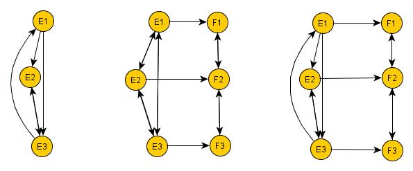
Figure 1: Mixed (left), chain graph (middle) and the mixed-chain graph (rigth) associated to an MHMM

In all the examples throughout the paper, we implicitly assume that each node of the mixed-chain graph, corresponding to a latent variable, is parent of itself, even if the edge $\mathbf{\circlearrowleft}$ is not reported.

Example 1

The mixed-chain graph on the right of Figure 2 encodes that the latent variables of the three dimensional MHMM are Granger caused reciprocally but are contemporaneously independent, i.e. $E_{1}(t)\mathchoice{\mathrel{\hbox to0.0pt{$\displaystyle\perp$\hss}\mkern 2.0mu{\displaystyle\perp}}}{\mathrel{\hbox to0.0pt{$\textstyle\perp$\hss}\mkern 2.0mu{\textstyle\perp}}}{\mathrel{\hbox to0.0pt{$\scriptstyle\perp$\hss}\mkern 2.0mu{\scriptstyle\perp}}}{\mathrel{\hbox to0.0pt{$\scriptscriptstyle\perp$\hss}\mkern 2.0mu{\scriptscriptstyle\perp}}}E_{2}(t)\mathchoice{\mathrel{\hbox to0.0pt{$\displaystyle\perp$\hss}\mkern 2.0mu{\displaystyle\perp}}}{\mathrel{\hbox to0.0pt{$\textstyle\perp$\hss}\mkern 2.0mu{\textstyle\perp}}}{\mathrel{\hbox to0.0pt{$\scriptstyle\perp$\hss}\mkern 2.0mu{\scriptstyle\perp}}}{\mathrel{\hbox to0.0pt{$\scriptscriptstyle\perp$\hss}\mkern 2.0mu{\scriptscriptstyle\perp}}}E_{3}(t)|E_{\{1,2,3\}}(t-1)$; moreover, every observable variable depends only on its own latent variable, i.e. $F_{1}(t)\mathchoice{\mathrel{\hbox to0.0pt{$\displaystyle\perp$\hss}\mkern 2.0mu{\displaystyle\perp}}}{\mathrel{\hbox to0.0pt{$\textstyle\perp$\hss}\mkern 2.0mu{\textstyle\perp}}}{\mathrel{\hbox to0.0pt{$\scriptstyle\perp$\hss}\mkern 2.0mu{\scriptstyle\perp}}}{\mathrel{\hbox to0.0pt{$\scriptscriptstyle\perp$\hss}\mkern 2.0mu{\scriptscriptstyle\perp}}}E_{\{2,3\}}(t)|E_{1}(t)$, $F_{2}(t)\mathchoice{\mathrel{\hbox to0.0pt{$\displaystyle\perp$\hss}\mkern 2.0mu{\displaystyle\perp}}}{\mathrel{\hbox to0.0pt{$\textstyle\perp$\hss}\mkern 2.0mu{\textstyle\perp}}}{\mathrel{\hbox to0.0pt{$\scriptstyle\perp$\hss}\mkern 2.0mu{\scriptstyle\perp}}}{\mathrel{\hbox to0.0pt{$\scriptscriptstyle\perp$\hss}\mkern 2.0mu{\scriptscriptstyle\perp}}}E_{\{1,3\}}(t)|E_{2}(t)$, $F_{3}(t)\mathchoice{\mathrel{\hbox to0.0pt{$\displaystyle\perp$\hss}\mkern 2.0mu{\displaystyle\perp}}}{\mathrel{\hbox to0.0pt{$\textstyle\perp$\hss}\mkern 2.0mu{\textstyle\perp}}}{\mathrel{\hbox to0.0pt{$\scriptstyle\perp$\hss}\mkern 2.0mu{\scriptstyle\perp}}}{\mathrel{\hbox to0.0pt{$\scriptscriptstyle\perp$\hss}\mkern 2.0mu{\scriptscriptstyle\perp}}}E_{\{1,2\}}(t)|E_{3}(t)$, $F_{\{1,2\}}(t)$ $\mathchoice{\mathrel{\hbox to0.0pt{$\displaystyle\perp$\hss}\mkern 2.0mu{\displaystyle\perp}}}{\mathrel{\hbox to0.0pt{$\textstyle\perp$\hss}\mkern 2.0mu{\textstyle\perp}}}{\mathrel{\hbox to0.0pt{$\scriptstyle\perp$\hss}\mkern 2.0mu{\scriptstyle\perp}}}{\mathrel{\hbox to0.0pt{$\scriptscriptstyle\perp$\hss}\mkern 2.0mu{\scriptscriptstyle\perp}}}E_{3}(t)|E_{\{1,2\}}(t)$, $F_{\{2,3\}}(t)\mathchoice{\mathrel{\hbox to0.0pt{$\displaystyle\perp$\hss}\mkern 2.0mu{\displaystyle\perp}}}{\mathrel{\hbox to0.0pt{$\textstyle\perp$\hss}\mkern 2.0mu{\textstyle\perp}}}{\mathrel{\hbox to0.0pt{$\scriptstyle\perp$\hss}\mkern 2.0mu{\scriptstyle\perp}}}{\mathrel{\hbox to0.0pt{$\scriptscriptstyle\perp$\hss}\mkern 2.0mu{\scriptscriptstyle\perp}}}E_{1}(t)|E_{\{2,3\}}(t)$, $F_{\{1,3\}}(t)\mathchoice{\mathrel{\hbox to0.0pt{$\displaystyle\perp$\hss}\mkern 2.0mu{\displaystyle\perp}}}{\mathrel{\hbox to0.0pt{$\textstyle\perp$\hss}\mkern 2.0mu{\textstyle\perp}}}{\mathrel{\hbox to0.0pt{$\scriptstyle\perp$\hss}\mkern 2.0mu{\scriptstyle\perp}}}{\mathrel{\hbox to0.0pt{$\scriptscriptstyle\perp$\hss}\mkern 2.0mu{\scriptscriptstyle\perp}}}E_{2}(t)|E_{\{1,3\}}(t)$; and, at every time point, the observable variables given the latent states are independent, i.e. $F_{1}(t)\mathchoice{\mathrel{\hbox to0.0pt{$\displaystyle\perp$\hss}\mkern 2.0mu{\displaystyle\perp}}}{\mathrel{\hbox to0.0pt{$\textstyle\perp$\hss}\mkern 2.0mu{\textstyle\perp}}}{\mathrel{\hbox to0.0pt{$\scriptstyle\perp$\hss}\mkern 2.0mu{\scriptstyle\perp}}}{\mathrel{\hbox to0.0pt{$\scriptscriptstyle\perp$\hss}\mkern 2.0mu{\scriptscriptstyle\perp}}}F_{2}(t)\mathchoice{\mathrel{\hbox to0.0pt{$\displaystyle\perp$\hss}\mkern 2.0mu{\displaystyle\perp}}}{\mathrel{\hbox to0.0pt{$\textstyle\perp$\hss}\mkern 2.0mu{\textstyle\perp}}}{\mathrel{\hbox to0.0pt{$\scriptstyle\perp$\hss}\mkern 2.0mu{\scriptstyle\perp}}}{\mathrel{\hbox to0.0pt{$\scriptscriptstyle\perp$\hss}\mkern 2.0mu{\scriptscriptstyle\perp}}}F_{3}(t)|E_{\{1,2,3\}}(t)$.

The mixed-chain graph on the left of Figure 2 is associated to a 3-variate MHMM where the latent variables are not contemporaneously independent, and each of them depends only on its own past, i.e. the encoded Granger noncausality conditions (7) are $E_{1}(t)\mathchoice{\mathrel{\hbox to0.0pt{$\displaystyle\perp$\hss}\mkern 2.0mu{\displaystyle\perp}}}{\mathrel{\hbox to0.0pt{$\textstyle\perp$\hss}\mkern 2.0mu{\textstyle\perp}}}{\mathrel{\hbox to0.0pt{$\scriptstyle\perp$\hss}\mkern 2.0mu{\scriptstyle\perp}}}{\mathrel{\hbox to0.0pt{$\scriptscriptstyle\perp$\hss}\mkern 2.0mu{\scriptscriptstyle\perp}}}E_{\{2,3\}}(t-1)|E_{1}(t-1)$, $E_{2}(t)\mathchoice{\mathrel{\hbox to0.0pt{$\displaystyle\perp$\hss}\mkern 2.0mu{\displaystyle\perp}}}{\mathrel{\hbox to0.0pt{$\textstyle\perp$\hss}\mkern 2.0mu{\textstyle\perp}}}{\mathrel{\hbox to0.0pt{$\scriptstyle\perp$\hss}\mkern 2.0mu{\scriptstyle\perp}}}{\mathrel{\hbox to0.0pt{$\scriptscriptstyle\perp$\hss}\mkern 2.0mu{\scriptscriptstyle\perp}}}E_{\{1,3\}}(t-1)|E_{2}(t-1)$, $E_{3}(t)\mathchoice{\mathrel{\hbox to0.0pt{$\displaystyle\perp$\hss}\mkern 2.0mu{\displaystyle\perp}}}{\mathrel{\hbox to0.0pt{$\textstyle\perp$\hss}\mkern 2.0mu{\textstyle\perp}}}{\mathrel{\hbox to0.0pt{$\scriptstyle\perp$\hss}\mkern 2.0mu{\scriptstyle\perp}}}{\mathrel{\hbox to0.0pt{$\scriptscriptstyle\perp$\hss}\mkern 2.0mu{\scriptscriptstyle\perp}}}E_{\{1,2\}}(t-1)|E_{3}(t-1)$, $E_{\{1,2\}}(t)\mathchoice{\mathrel{\hbox to0.0pt{$\displaystyle\perp$\hss}\mkern 2.0mu{\displaystyle\perp}}}{\mathrel{\hbox to0.0pt{$\textstyle\perp$\hss}\mkern 2.0mu{\textstyle\perp}}}{\mathrel{\hbox to0.0pt{$\scriptstyle\perp$\hss}\mkern 2.0mu{\scriptstyle\perp}}}{\mathrel{\hbox to0.0pt{$\scriptscriptstyle\perp$\hss}\mkern 2.0mu{\scriptscriptstyle\perp}}}E_{3}(t-1)|E_{\{1,2\}}(t-1)$, $E_{\{2,3\}}(t)\mathchoice{\mathrel{\hbox to0.0pt{$\displaystyle\perp$\hss}\mkern 2.0mu{\displaystyle\perp}}}{\mathrel{\hbox to0.0pt{$\textstyle\perp$\hss}\mkern 2.0mu{\textstyle\perp}}}{\mathrel{\hbox to0.0pt{$\scriptstyle\perp$\hss}\mkern 2.0mu{\scriptstyle\perp}}}{\mathrel{\hbox to0.0pt{$\scriptscriptstyle\perp$\hss}\mkern 2.0mu{\scriptscriptstyle\perp}}}E_{1}(t-1)|E_{\{2,3\}}(t-1)$, $E_{\{1,3\}}(t)\mathchoice{\mathrel{\hbox to0.0pt{$\displaystyle\perp$\hss}\mkern 2.0mu{\displaystyle\perp}}}{\mathrel{\hbox to0.0pt{$\textstyle\perp$\hss}\mkern 2.0mu{\textstyle\perp}}}{\mathrel{\hbox to0.0pt{$\scriptstyle\perp$\hss}\mkern 2.0mu{\scriptstyle\perp}}}{\mathrel{\hbox to0.0pt{$\scriptscriptstyle\perp$\hss}\mkern 2.0mu{\scriptscriptstyle\perp}}}E_{2}(t-1)|E_{\{1,3\}}(t-1)$; while the independence conditions (10) of manifest from latent variables are $F_{\{1,2\}}(t)\mathchoice{\mathrel{\hbox to0.0pt{$\displaystyle\perp$\hss}\mkern 2.0mu{\displaystyle\perp}}}{\mathrel{\hbox to0.0pt{$\textstyle\perp$\hss}\mkern 2.0mu{\textstyle\perp}}}{\mathrel{\hbox to0.0pt{$\scriptstyle\perp$\hss}\mkern 2.0mu{\scriptstyle\perp}}}{\mathrel{\hbox to0.0pt{$\scriptscriptstyle\perp$\hss}\mkern 2.0mu{\scriptscriptstyle\perp}}}E_{3}(t)|E_{\{1,2\}}(t)$ and $F_{3}(t)\mathchoice{\mathrel{\hbox to0.0pt{$\displaystyle\perp$\hss}\mkern 2.0mu{\displaystyle\perp}}}{\mathrel{\hbox to0.0pt{$\textstyle\perp$\hss}\mkern 2.0mu{\textstyle\perp}}}{\mathrel{\hbox to0.0pt{$\scriptstyle\perp$\hss}\mkern 2.0mu{\scriptstyle\perp}}}{\mathrel{\hbox to0.0pt{$\scriptscriptstyle\perp$\hss}\mkern 2.0mu{\scriptscriptstyle\perp}}}E_{\{1,2\}}(t)|E_{3}(t)$; the local independence (9) is $F_{1}(t)\mathchoice{\mathrel{\hbox to0.0pt{$\displaystyle\perp$\hss}\mkern 2.0mu{\displaystyle\perp}}}{\mathrel{\hbox to0.0pt{$\textstyle\perp$\hss}\mkern 2.0mu{\textstyle\perp}}}{\mathrel{\hbox to0.0pt{$\scriptstyle\perp$\hss}\mkern 2.0mu{\scriptstyle\perp}}}{\mathrel{\hbox to0.0pt{$\scriptscriptstyle\perp$\hss}\mkern 2.0mu{\scriptscriptstyle\perp}}}F_{\{2,3\}}(t)|E_{\{1,2,3\}}(t)$.

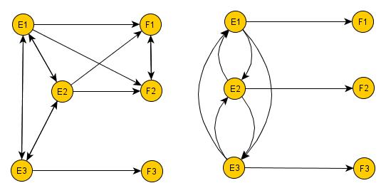
Figure 2: Mixed-chain graphs associated to MHMMs

Example 2

(MHMMs for marketing and financial data). The mixed-chain graph on the left in Figure 3 is associated to an MHMM encoding the dynamic relations of three observable time series which depend on two latent factors. The observable time series can represent, for example, the sales levels of three products that can be interpreted as indicators of the motivational latent states of the customers behaviors. The distributions of the motivational states may be of interest more than those of the product sales. The graph underlies that the first two products belong to the same category so their sales series ($F_{1},F_{2}$) depend on the latent variable $E_{1}$ $(i.e.\ F_{\{1,2\}}(t)\mathchoice{\mathrel{\hbox to0.0pt{$\displaystyle\perp$\hss}\mkern 2.0mu{\displaystyle\perp}}}{\mathrel{\hbox to0.0pt{$\textstyle\perp$\hss}\mkern 2.0mu{\textstyle\perp}}}{\mathrel{\hbox to0.0pt{$\scriptstyle\perp$\hss}\mkern 2.0mu{\scriptstyle\perp}}}{\mathrel{\hbox to0.0pt{$\scriptscriptstyle\perp$\hss}\mkern 2.0mu{\scriptscriptstyle\perp}}}E_{2}(t)|E_{1}(t))$, the sales of the third product respond to a different latent variable $E_{2}$ $(i.e.\ F_{3}(t)\mathchoice{\mathrel{\hbox to0.0pt{$\displaystyle\perp$\hss}\mkern 2.0mu{\displaystyle\perp}}}{\mathrel{\hbox to0.0pt{$\textstyle\perp$\hss}\mkern 2.0mu{\textstyle\perp}}}{\mathrel{\hbox to0.0pt{$\scriptstyle\perp$\hss}\mkern 2.0mu{\scriptstyle\perp}}}{\mathrel{\hbox to0.0pt{$\scriptscriptstyle\perp$\hss}\mkern 2.0mu{\scriptscriptstyle\perp}}}E_{1}(t)|E_{2}(t))$; the observable sales levels are independent given the latent states $(i.e.\ F_{1}(t)\mathchoice{\mathrel{\hbox to0.0pt{$\displaystyle\perp$\hss}\mkern 2.0mu{\displaystyle\perp}}}{\mathrel{\hbox to0.0pt{$\textstyle\perp$\hss}\mkern 2.0mu{\textstyle\perp}}}{\mathrel{\hbox to0.0pt{$\scriptstyle\perp$\hss}\mkern 2.0mu{\scriptstyle\perp}}}{\mathrel{\hbox to0.0pt{$\scriptscriptstyle\perp$\hss}\mkern 2.0mu{\scriptscriptstyle\perp}}}F_{2}(t)\mathchoice{\mathrel{\hbox to0.0pt{$\displaystyle\perp$\hss}\mkern 2.0mu{\displaystyle\perp}}}{\mathrel{\hbox to0.0pt{$\textstyle\perp$\hss}\mkern 2.0mu{\textstyle\perp}}}{\mathrel{\hbox to0.0pt{$\scriptstyle\perp$\hss}\mkern 2.0mu{\scriptstyle\perp}}}{\mathrel{\hbox to0.0pt{$\scriptscriptstyle\perp$\hss}\mkern 2.0mu{\scriptscriptstyle\perp}}}F_{3}(t)|E_{\{1,2\}}(t))$; the two motivational latent processes are G-caused reciprocally, so that the past motivational states influence the actual state of each latent variable, but they are contemporaneously independent $(i.e.\ E_{1}(t)\mathchoice{\mathrel{\hbox to0.0pt{$\displaystyle\perp$\hss}\mkern 2.0mu{\displaystyle\perp}}}{\mathrel{\hbox to0.0pt{$\textstyle\perp$\hss}\mkern 2.0mu{\textstyle\perp}}}{\mathrel{\hbox to0.0pt{$\scriptstyle\perp$\hss}\mkern 2.0mu{\scriptstyle\perp}}}{\mathrel{\hbox to0.0pt{$\scriptscriptstyle\perp$\hss}\mkern 2.0mu{\scriptscriptstyle\perp}}}E_{2}(t)|E_{\{1,2\}}(t-1))$.

The mixed-chain graph on the right in Figure 3 can describe a model for financial series where specific and generic latent effects exist. The series $F_{1},F_{2}$ can indicate the trading patterns of two financial traded shares in two different financial sectors. The presence or the absence of trading may depend on a specific latent aspect typical of each financial sector where the trading takes place (e.g. the turbulence of the sector), so each observable variable depends on one specific latent variable: $F_{1}$ on $E_{1}$, $F_{2}$ on $E_{2}$, but all the trading patterns may be influenced by one common unobservable variable ($E_{3}$) such as the Market turbulence with states that correspond to calm or turbulent phases of the Market $(i.e.\ F_{1}(t)\mathchoice{\mathrel{\hbox to0.0pt{$\displaystyle\perp$\hss}\mkern 2.0mu{\displaystyle\perp}}}{\mathrel{\hbox to0.0pt{$\textstyle\perp$\hss}\mkern 2.0mu{\textstyle\perp}}}{\mathrel{\hbox to0.0pt{$\scriptstyle\perp$\hss}\mkern 2.0mu{\scriptstyle\perp}}}{\mathrel{\hbox to0.0pt{$\scriptscriptstyle\perp$\hss}\mkern 2.0mu{\scriptscriptstyle\perp}}}E_{2}(t)|E_{\{1,3\}}(t),F_{2}(t)\mathchoice{\mathrel{\hbox to0.0pt{$\displaystyle\perp$\hss}\mkern 2.0mu{\displaystyle\perp}}}{\mathrel{\hbox to0.0pt{$\textstyle\perp$\hss}\mkern 2.0mu{\textstyle\perp}}}{\mathrel{\hbox to0.0pt{$\scriptstyle\perp$\hss}\mkern 2.0mu{\scriptstyle\perp}}}{\mathrel{\hbox to0.0pt{$\scriptscriptstyle\perp$\hss}\mkern 2.0mu{\scriptscriptstyle\perp}}}E_{1}(t)|E_{\{2,3\}}(t))$. There is local independence $F_{1}(t)\mathchoice{\mathrel{\hbox to0.0pt{$\displaystyle\perp$\hss}\mkern 2.0mu{\displaystyle\perp}}}{\mathrel{\hbox to0.0pt{$\textstyle\perp$\hss}\mkern 2.0mu{\textstyle\perp}}}{\mathrel{\hbox to0.0pt{$\scriptstyle\perp$\hss}\mkern 2.0mu{\scriptstyle\perp}}}{\mathrel{\hbox to0.0pt{$\scriptscriptstyle\perp$\hss}\mkern 2.0mu{\scriptscriptstyle\perp}}}F_{2}(t)|E_{\{1,2,3\}}(t)$. Moreover, the past Market turbulence can affect the current turbulence of each financial sector (G-causality) whereas a specific latent variable of a sector does not Granger cause the other specific latent variable and the turbolence of the Market, $(i.e.\ E_{3}(t)\mathchoice{\mathrel{\hbox to0.0pt{$\displaystyle\perp$\hss}\mkern 2.0mu{\displaystyle\perp}}}{\mathrel{\hbox to0.0pt{$\textstyle\perp$\hss}\mkern 2.0mu{\textstyle\perp}}}{\mathrel{\hbox to0.0pt{$\scriptstyle\perp$\hss}\mkern 2.0mu{\scriptstyle\perp}}}{\mathrel{\hbox to0.0pt{$\scriptscriptstyle\perp$\hss}\mkern 2.0mu{\scriptscriptstyle\perp}}}E_{\{1,2\}}(t-1)|E_{3}(t-1),E_{\{1,3\}}(t)\mathchoice{\mathrel{\hbox to0.0pt{$\displaystyle\perp$\hss}\mkern 2.0mu{\displaystyle\perp}}}{\mathrel{\hbox to0.0pt{$\textstyle\perp$\hss}\mkern 2.0mu{\textstyle\perp}}}{\mathrel{\hbox to0.0pt{$\scriptstyle\perp$\hss}\mkern 2.0mu{\scriptstyle\perp}}}{\mathrel{\hbox to0.0pt{$\scriptscriptstyle\perp$\hss}\mkern 2.0mu{\scriptscriptstyle\perp}}}E_{2}(t-1)|E_{\{1,3\}}(t-1),E_{\{2,3\}}(t)\mathchoice{\mathrel{\hbox to0.0pt{$\displaystyle\perp$\hss}\mkern 2.0mu{\displaystyle\perp}}}{\mathrel{\hbox to0.0pt{$\textstyle\perp$\hss}\mkern 2.0mu{\textstyle\perp}}}{\mathrel{\hbox to0.0pt{$\scriptstyle\perp$\hss}\mkern 2.0mu{\scriptstyle\perp}}}{\mathrel{\hbox to0.0pt{$\scriptscriptstyle\perp$\hss}\mkern 2.0mu{\scriptscriptstyle\perp}}}E_{1}(t-1)|E_{\{2,3\}}(t-1))$. Finally there is no contemporaneous relation among the three turbulences $(i.e.\ E_{1}(t)\mathchoice{\mathrel{\hbox to0.0pt{$\displaystyle\perp$\hss}\mkern 2.0mu{\displaystyle\perp}}}{\mathrel{\hbox to0.0pt{$\textstyle\perp$\hss}\mkern 2.0mu{\textstyle\perp}}}{\mathrel{\hbox to0.0pt{$\scriptstyle\perp$\hss}\mkern 2.0mu{\scriptstyle\perp}}}{\mathrel{\hbox to0.0pt{$\scriptscriptstyle\perp$\hss}\mkern 2.0mu{\scriptscriptstyle\perp}}}E_{2}(t)\mathchoice{\mathrel{\hbox to0.0pt{$\displaystyle\perp$\hss}\mkern 2.0mu{\displaystyle\perp}}}{\mathrel{\hbox to0.0pt{$\textstyle\perp$\hss}\mkern 2.0mu{\textstyle\perp}}}{\mathrel{\hbox to0.0pt{$\scriptstyle\perp$\hss}\mkern 2.0mu{\scriptstyle\perp}}}{\mathrel{\hbox to0.0pt{$\scriptscriptstyle\perp$\hss}\mkern 2.0mu{\scriptscriptstyle\perp}}}E_{3}(t)|E_{\{1,2,3\}}(t-1))$.

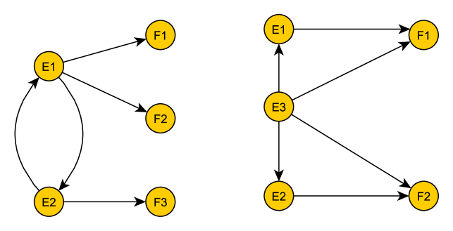
Figure 3: Mixed-chain graphs associated to MHMMs for marketing and financial data illustrated in Example 2

Two final remarks can be advisable. First, one immediate consequence of Theorem 1 and Definition 3 is the following result

Corollary 1

If the MHMM $(\mathbf{E_{\mathcal{U}}},\mathbf{F}_{\mathcal{V}})$ is Markov wrt a mixed graph $G$ and a chain graph $G^{*}$, such that $pa_{G}(\mathcal{T})=\mathcal{T}$ and $pa_{G^{*}}(\mathcal{R})=\mathcal{T}$, then the marginal process $(\mathbf{E_{\mathcal{T}}},\mathbf{F}_{\mathcal{R}})$, $\mathcal{T}\subset\mathcal{U}$, $\mathcal{R}\subset\mathcal{V}$, is an MHMM.

Proof. Conditions (7) and (10) for $(\mathbf{E_{\mathcal{U}}},\mathbf{F}_{\mathcal{V}})$ being Markov with respect to the graphs where $pa_{G}(\mathcal{T})=\mathcal{T}$ and $pa_{G^{*}}(\mathcal{R})=\mathcal{T}$ coincide with the conditions (1) and (2) ensuring that $(\mathbf{E_{\mathcal{T}}},\mathbf{F}_{\mathcal{R}})$,$\mathcal{T}\subset\mathcal{U}$, $\mathcal{R}\subset\mathcal{V}$, is still a hidden process.

Moreover, the restrictions which the observation and latent models obey in linked and coupled MHMMs (Definition 2) can be described by the Markov properties of mixed and chain graphs as specified in the corollary below.

Corollary 2

An MHMM $(\mathbf{E_{\mathcal{U}}},\mathbf{F}_{\mathcal{V}})$ which is Markov wrt a mixed graph $G$ and a chain graph $G^{*}$ is a linked MHMM with $l$ components if, for a partition of the latent variables $\mbox{${\cal U}$}=\bigcup_{i=1}^{l}\mbox{${\cal T}$}_{i}$ and a partition of of the observable variables $\mbox{${\cal V}$}=\bigcup_{i=1}^{l}\mbox{${\cal R}$}_{i}$, $i=1,...,l$, it holds that: $pa_{G}(\mathcal{T}_{i})=\mathcal{T}_{i}$, $pa_{G^{*}}(\mathcal{R}_{i})=\mathcal{T}_{i}$ and $sp_{G^{*}}(\mathcal{R}_{i})=\mathcal{R}_{i}.$ If the condition $pa_{G}(\mathcal{T}_{i})=\mathcal{T}_{i}$ is replaced by $sp_{G}(\mathcal{T}_{i})=\mathcal{T}_{i}$, the process $(\mathbf{E_{\mathcal{U}}},\mathbf{F}_{\mathcal{V}})$ Markov wrt such graphs is a coupled MHMM.

The proof is omitted as similar to that of Corollary 1.

For instance, in Figure 2, the mixed-chain graph on the left corresponds to a linked MHMM with two components and the mixed-chain graph on the right to a coupled MHMM with three components.

3.2 Equivalent mixed-chain graphs

Standard hidden Markov models, and more in general mixture models, suffer from the non-identifiability problem due to the invariance with respect to relabeling of hidden states. For this reason, MHMMs are identifiable only up to switching the latent categories and the labels of the latent variables. Due to the invariance with respect to switching labels of the latent variables, there are mixed-chain graphs equivalent in the sense that they correspond to the same MHMM. We now clarify this point thoroughly.

Two mixed-chain graphs, say $G_{1}$ and $G_{2}$, with the same sets of nodes, are equivalent if there is a bijection $\nu$ which maps the set of nodes corresponding to the latent variables onto itself assuring that: i) the nodes $E_{i}$ of $G_{1}$and $\nu(E_{i})$ of $G_{2}$ are associated to latent variables with the same number of states; ii) if $E_{i}$, $E_{j}$ are connected by an edge in $G_{1}$ then $\nu(E_{i})$ and $\nu(E_{j})$ are connected by the same type of edge in $G_{2}$; iii) if $E_{i}$, $E_{j}$ are not connected by any edges in $G_{1}$ then $\nu(E_{i})$ and $\nu(E_{j})$ are not connected in $G_{2}$; iv) if $E_{i}$ is a parent of $F_{j}$ in $G_{1}$ then $\nu(E_{i})$ is a parent of $F_{j}$ in $G_{2}$.

It is evident that two mixed-chain graphs, equivalent according to the previous conditions, encode conditional independencies that differ only for the labels assigned to the latent variables.

An example illustrates the mentioned concepts.

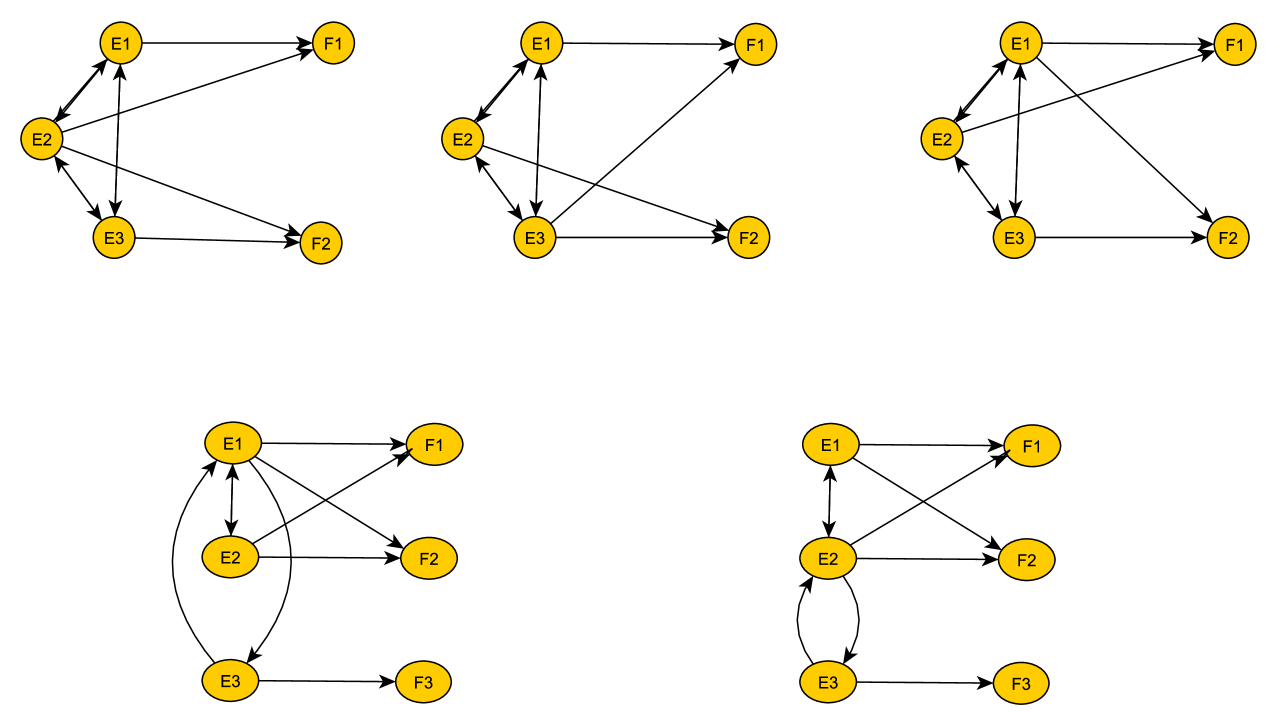
Figure 4: Equivalent mixed-chain graphs

Example 3

The first line of Figure 4 shows three equivalent mixed-chain graphs corresponding to an MHMM where a latent variable affects both the observable variables (generic latent effect) and each manifest variable is governed by its specific latent variable (specific latent effect). In the second line of Figure 4, the two equivalent mixed-chain graphs identify the MHMM where two latent variables affect only the first two observable variables and another latent variable is specific for the third observable variable. Moreover, the latent variable specific for $F_{3}$ is contemporaneously independent of the other two latent variables, and there is no Granger-causality between this variable and one of the remaining unobservable variables.

4 A parameterization for MHMMs

Till now we have described the hypotheses underlying MHMMs, now we need to illustrate how to test such hypotheses. In particular, all the conditional independencies so far illustrated are related to the natural parameters of the MHMMs: the probabilities of the observable variables given the latent states and the transition probabilities of the latent process.

The time-homogeneous joint transition probabilities are denoted by $\phi(\emph{{\text{e}}}|\emph{{\text{e}}}^{\prime})$ for every pair of states $\emph{{\text{e}}}^{\prime}\in\mathcal{E}$, $\emph{{\text{e}}}\in\mathcal{E}$. Moreover, $\phi_{\mathcal{T}}(\emph{{\text{e}}}_{\mathcal{T}}|\emph{{\text{e}}}^{\prime})$ is the marginal transition probability from state $\emph{{\text{e}}}^{\prime}\in\mathcal{E}$ to state $\emph{{\text{e}}}_{\mathcal{T}}$ with components $e_{i}:i\in\mathcal{T}\subset\mathcal{U}$. We assume that the initial distribution of $\mathbf{E}_{\mathcal{U}}$ is the invariant one and is unique. Finally, $\varphi(\emph{{f}}|\emph{{e}})$ indicates the state-dependent distribution that is the conditional probabilities of the observable variables given the latent state e and $\varphi_{\mathcal{R}}(\emph{{f}}_{\mathcal{R}}|\emph{{e}})$ represents the marginal probability of the observable variables in the set $\mathcal{R}$ given the latent state e.

In this section, we propose to parameterize both the state-dependent distributions and the transition probabilities of the latent process through marginal models and verify hypotheses which make these models more parsimonious by constraining marginal parameters. In the marginal models, the parameters are called marginal interactions. In particular, marginal interactions are log-linear parameters defined in different marginal distributions in Bergsma and Rudas (2002) models, while Bartolucci et al., 2007, use more general marginal interactions which are meaningful when the variables have an ordinal nature. Here, we adopt a Gloneck-McCullagh multivariate logistic model (Gloneck and McCullagh, 1995) whose interactions, involving the variables in the set $\mathcal{P}$, are log-linear parameters defined on the marginal distributions $\phi_{\mathcal{P}}(\textbf{\emph{e}}_{\mathcal{P}}|\textbf{\emph{e}}^{\prime})$, $\varphi_{\mathcal{P}}(\textbf{\emph{f}}_{\mathcal{P}}|\textbf{\emph{e}})$.

For every observable or latent categorical variable, the first category is called baseline. Any observation $\textbf{\emph{f}}=(f_{1},f_{2},...,f_{s})$ which includes categories at the baseline level for variables $j\notin\mathcal{J}$, $\mathcal{J}\subset\mathcal{V},$ is denoted by $(\emph{{\text{f}}}_{\mathcal{J}},\emph{{\text{f*}}}_{\mathcal{{V}}\setminus\mathcal{J}})$. A similar notation holds for the latent state $\textbf{\emph{e}}=(e_{1},e_{2},...,e_{r})$. For every non-empty subset $\mathcal{P}$ of the observable variables $\mathcal{V}$ and for every $\emph{{\text{f}}}_{\mathcal{P}}\in\times_{j\in\mathcal{P}}\mathcal{F}_{j}$, the baseline interactions $\eta^{\mathcal{P}}(\emph{{\text{f}}}_{\mathcal{P}}|\emph{{\text{e}}})$, $\mathcal{P}\in\mathcal{V}$, of the Gloneck-McCullagh marginal model for the observable variables are contrasts of logarithms of marginal state-dependent probabilities

$$\eta^{\mathcal{P}}(\emph{{\text{f}}}_{\mathcal{P}}|\emph{{\text{e}}})=\sum_{\mathcal{K}\subseteq\mathcal{P}}(-1)^{|\mathcal{P}\backslash\mathcal{K}|}\log\varphi_{\mathcal{P}}(\emph{{\text{f}}}_{\mathcal{K}},\emph{{\text{f*}}}_{\mathcal{P}\setminus\mathcal{K}}|\emph{{\text{e}}}).$$

In order to model the dependence of the distribution of the observable variables on the states e, we adopt the usual factorial expansion

$$\eta^{\mathcal{P}}(\emph{{\text{f}}}_{\mathcal{P}}|\emph{{\text{e}}})=\sum_{\mathcal{Q}\subseteq\mathcal{U}}\theta^{\mathcal{P},\mathcal{Q}}(\emph{{\text{f}}}_{\mathcal{P}}|\emph{{\text{e}}}_{\mathcal{Q}}).$$ (11)

Analogously, in the marginal model for the latent component of MHMMs, we define, for every $\mathcal{P}\subseteq\mathcal{U}$, the marginal parameters

$$\lambda^{\mathcal{P}}(\emph{{\text{e}}}_{\mathcal{P}}|\emph{{\text{e}}}^{\prime})=\sum_{\mathcal{K}\subseteq\mathcal{P}}(-1)^{|\mathcal{P}\backslash\mathcal{K}|}\log\phi_{\mathcal{P}}(\emph{{\text{e}}}_{\mathcal{P}}|\emph{{\text{e}}}^{\prime}).$$

and the factorial expansion

$$\lambda^{\mathcal{P}}(\emph{{\text{e}}}_{\mathcal{P}}|\emph{{\text{e}}}^{\prime})=\sum_{\mathcal{Q}\subseteq\mathcal{U}}\delta^{\mathcal{P},\mathcal{Q}}(\emph{{\text{e}}}_{\mathcal{P}}|\emph{{\text{e}}}^{\prime}_{\mathcal{Q}}).$$ (12)

4.1 Parametric constraints for conditional independencies

The properties of graphical models for MHMMs (Definition 3) correspond to zero restrictions on the parameters $\theta^{\mathcal{P},\mathcal{Q}}(\emph{{{f}}}_{\mathcal{P}}|\emph{{{e}}}_{\mathcal{Q}})$ and $\delta^{\mathcal{P},\mathcal{Q}}(\emph{{{e}}}_{\mathcal{P}}|\emph{{{e}}}^{\prime}_{\mathcal{Q}})$, introduced in (11) and (12), as illustrated in the next theorem.

Theorem 2

For a latent model with strictly positive time-homogeneous transition probabilities, the Granger noncausality condition (7) is equivalent to $\delta^{\mathcal{P},\mathcal{Q}}({\textbf{{e}}}_{\mathcal{P}}|{\textbf{{e}}}^{\prime}_{\mathcal{Q}})=\mathbf{0}$ for all $\mathcal{P}\subseteq\mathcal{T},\mathcal{Q}\not\subseteq pa_{G}(\mathcal{P})$, while the conditional contemporaneous independence (8) is equivalent to $\delta^{\mathcal{P},\mathcal{Q}}({\textbf{{e}}}_{\mathcal{P}}|{\textbf{{e}}}^{\prime}_{\mathcal{Q}})=\mathbf{0}$ for all $\mathcal{P}\not\in\mathfrak{B}(G)$, $\textbf{{e}}_{\mathcal{P}}\in\times_{i\in\mathcal{P}}\mathcal{E}_{i}$, $\textbf{{e}}^{\prime}_{\mathcal{Q}}\in\times_{i\in\mathcal{Q}}\mathcal{E}_{i}$.

Moreover, if the state-dependent probabilities are strictly positive, the independence (9) is equivalent to $\theta^{\mathcal{P},\mathcal{Q}}({\textbf{{f}}}_{\mathcal{P}}|{\textbf{{e}}}_{\mathcal{Q}})=\mathbf{0}$ for all $\mathcal{P}\not\in\mathfrak{B}(G^{*})$, while condition (10) corresponds to $\theta^{\mathcal{P},\mathcal{Q}}({\textbf{{f}}}_{\mathcal{P}}|{\textbf{{e}}}_{\mathcal{Q}})=\mathbf{0}$ for all $\mathcal{P}\subseteq\mathcal{R}$, $\mathcal{Q}\not\subseteq pa_{G^{*}}(\mathcal{P})$, $\textbf{{f}}_{\mathcal{P}}\in\times_{j\in\mathcal{P}}\mathcal{F}_{j}$, $\textbf{{e}}_{\mathcal{Q}}\in\times_{i\in\mathcal{Q}}\mathcal{E}_{i}$.

Proof. The equivalence between the zero restrictions on $\delta$ parameters and conditions (7) and (8) follows from Colombi and Giordano, 2012, the nullity of $\theta$ parameters under the conditions (9) and (10) from Marchetti and Lupparelli, 2011.

The theorem allows a simple implementation of standard methods to fit and test MHMMs under the restrictions (7, 8, 9, 10). The theorem enhances the use of the marginal parametrization since all the conditions (7, 8, 9, 10) are equivalent to linear constraints on the marginal parameters, the same restrictions under the log-linear parametrization would correspond to non linear constraints on the parameters.

Moreover, since Corollary 1 proves that conditions (1) and (2) are particular cases of the independencies (7) and (10), the constraints on marginal parameters described in Theorem 2 are useful also for testing if the properties of an MHMM are preserved after marginalizing the latent and observable processes.

An example clarifies which marginal parameters are restricted to zero in order to satisfy the conditional independencies that correspond to the Markov properties of the mixed-chain graph.

Example 4

The left mixed-chain graph of Figure 5 encodes the following Markov properties: $E_{1}(t)\mathchoice{\mathrel{\hbox to0.0pt{$\displaystyle\perp$\hss}\mkern 2.0mu{\displaystyle\perp}}}{\mathrel{\hbox to0.0pt{$\textstyle\perp$\hss}\mkern 2.0mu{\textstyle\perp}}}{\mathrel{\hbox to0.0pt{$\scriptstyle\perp$\hss}\mkern 2.0mu{\scriptstyle\perp}}}{\mathrel{\hbox to0.0pt{$\scriptscriptstyle\perp$\hss}\mkern 2.0mu{\scriptscriptstyle\perp}}}E_{2}(t-1)|E_{1}(t-1)$ so that $E_{1}$ is no Granger caused by $E_{2}$ and $F_{i}(t)\mathchoice{\mathrel{\hbox to0.0pt{$\displaystyle\perp$\hss}\mkern 2.0mu{\displaystyle\perp}}}{\mathrel{\hbox to0.0pt{$\textstyle\perp$\hss}\mkern 2.0mu{\textstyle\perp}}}{\mathrel{\hbox to0.0pt{$\scriptstyle\perp$\hss}\mkern 2.0mu{\scriptstyle\perp}}}{\mathrel{\hbox to0.0pt{$\scriptscriptstyle\perp$\hss}\mkern 2.0mu{\scriptscriptstyle\perp}}}E_{j}(t)|E_{i}(t)$ for $i,j=1,2,$ $i\neq j$ which reveals a specific effect of the first (second) latent variable on the first (second) observable variable. According to Theorem 1, these conditions ensure that the marginal process $(\mathbf{E}_{{1}}$, $\mathbf{F}_{{1}})$ of the MHMM is still hidden Markov, but $(\mathbf{E}_{{2}}$, $\mathbf{F}_{{2}})$ is not. Moreover, the local independence condition $F_{1}(t)\mathchoice{\mathrel{\hbox to0.0pt{$\displaystyle\perp$\hss}\mkern 2.0mu{\displaystyle\perp}}}{\mathrel{\hbox to0.0pt{$\textstyle\perp$\hss}\mkern 2.0mu{\textstyle\perp}}}{\mathrel{\hbox to0.0pt{$\scriptstyle\perp$\hss}\mkern 2.0mu{\scriptstyle\perp}}}{\mathrel{\hbox to0.0pt{$\scriptscriptstyle\perp$\hss}\mkern 2.0mu{\scriptscriptstyle\perp}}}F_{2}(t)|E_{\{1,2\}}(t)$ can be also read off the same graph. The mentioned conditional independencies are equivalent to the nullity of the following parameters: $\theta^{1,2}({{{f}}}_{1}|{{{e_{2}}}})$, $\theta^{1,12}({{{f}}}_{1}|{{{e_{1},e_{2}}}})$, $\theta^{2,1}({{{f}}}_{2}|{{{e_{1}}}})$, $\theta^{2,12}({{{f}}}_{2}|{{{e_{1},e_{2}}}})$, $\theta^{12}({{{f}}}_{1},{{{f}}}_{2})$ $\theta^{12,1}({{{f}}}_{1},{{{f}}}_{2}|{{{e_{1}}}})$, $\theta^{12,2}({{{f}}}_{1},{{{f}}}_{2}|{{{e_{2}}}})$, $\theta^{12,12}({{{f}}}_{1},{{{f}}}_{2}|{{{e_{1},e_{2}}}})$, $\delta^{1,2}({{{e}}}_{1}|{{{e^{\prime}_{2}}}})$, $\delta^{1,2}({{{e}}}_{1}|{{{e^{\prime}_{1},e^{\prime}_{2}}}})$.

In the right graph of Figure 5 there is contemporaneous independence between the two latent variables, i.e. $E_{1}(t)\mathchoice{\mathrel{\hbox to0.0pt{$\displaystyle\perp$\hss}\mkern 2.0mu{\displaystyle\perp}}}{\mathrel{\hbox to0.0pt{$\textstyle\perp$\hss}\mkern 2.0mu{\textstyle\perp}}}{\mathrel{\hbox to0.0pt{$\scriptstyle\perp$\hss}\mkern 2.0mu{\scriptstyle\perp}}}{\mathrel{\hbox to0.0pt{$\scriptscriptstyle\perp$\hss}\mkern 2.0mu{\scriptscriptstyle\perp}}}E_{2}(t)|E_{1}(t-1)$ that is equivalent to the zero restrictions on $\delta^{12}({{{e}}}_{1},{{{e}}}_{2})$, $\delta^{12,1}({{{e}}}_{1},{{{e}}}_{2}|{{{e^{\prime}_{1}}}})$, $\delta^{12,2}({{{e}}}_{1},{{{e}}}_{2}|{{{e^{\prime}_{2}}}})$, $\delta^{12,12}({{{e}}}_{1},{{{e}}}_{2}|{{{e^{\prime}_{1},e^{\prime}_{2}}}})$. As for the left graph, the parameters $\theta^{12}({{{f}}}_{1},{{{f}}}_{2})$, $\theta^{12,1}({{{f}}}_{1},{{{f}}}_{2}|{{{e_{1}}}})$, $\theta^{12,2}({{{f}}}_{1},{{{f}}}_{2}|{{{e_{2}}}})$, $\theta^{12,12}({{{f}}}_{1},{{{f}}}_{2}|{{{e_{1},e_{2}}}})$ are null according to the local independence condition.

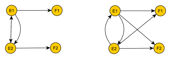
Figure 5: Mixed-chain graphs whose Markov properties correspond to the constraints on marginal parameters described in Example 4

4.2 Additivity hypotheses

In the framework of hidden Markov models with several latent and observable variables, other interesting hypotheses, that do not correspond to any conditional independence, can be easily formulated. These hypotheses reduce the number of parameters needed to parameterize the transition and observation probabilities. A useful restriction that considerably simplifies the observation model is the hypothesis of additivity of the effects of the latent variables on the marginal interactions of the observable variables. This marginal additive dependence allows the interactions to be expressed by the factorial expansion

$$\eta^{\mathcal{P}}(\emph{{\text{f}}}_{\mathcal{P}}|\emph{{\text{e}}})=\theta^{\mathcal{P}}(\emph{{\text{f}}}_{\mathcal{P}})+\sum_{k\in\mathcal{U}}\theta^{\mathcal{P},k}(\emph{{\text{f}}}_{\mathcal{P}}|\emph{{\text{e}}}_{k}).$$ (13)

Note that under this hypothesis, the parameters $\theta^{P,Q}(\emph{{\text{f}}}_{\mathcal{P}}|\emph{{\text{e}}}_{\mathcal{Q}})$ described in (11) are null if $|Q|>1.$ A similar additivity hypothesis can be used for the interactions of the latent model

$$\lambda^{\mathcal{P}}(\emph{{\text{e}}}_{\mathcal{P}}|\emph{{\text{e}}}^{\prime})=\delta^{\mathcal{P}}(\emph{{\text{e}}}_{\mathcal{P}})+\sum_{k\in\mathcal{U}}\delta^{\mathcal{P},k}(\emph{{\text{e}}}_{\mathcal{P}}|\emph{{\text{e}}}^{\prime}_{k}).$$ (14)

Another hypothesis is that of invariant association corresponding to the constraints $\eta^{\mathcal{P}}(\emph{{\text{f}}}_{\mathcal{P}}|\emph{{\text{e}}})=\theta^{\mathcal{P}}(\emph{{\text{f}}}_{\mathcal{P}})$, if $|P|>1$. According to this hypothesis the interactions between observable variables do not depend on the states of the latent variables.

Similarly, the constraints for the invariant association can be also imposed to the interactions of the latent model: $\lambda^{\mathcal{P}}(\emph{{\text{e}}}_{\mathcal{P}}|\emph{{\text{e}}}^{\prime})=\delta^{\mathcal{P}}(\emph{{\text{e}}}_{\mathcal{P}})$, if $|P|>1$.

5 Examples

In this section, we fit different MHMMs on two data sets. The EM algorithm used for estimating the models is described in Colombi and Giordano, 2011, and implemented in the R-package hmmm by Colombi et al., 2012.

The data set of a soft-drink company (Ching et al., 2002, available also in the R-package hmmm) consists of a one-year time series of daily sales of soft-drinks: lemon tea, orange juice and apple juice, all with categories: low, medium, high level. Changes in sale outcomes over time can depend on time-varying unobservable factors and we consider an MHMM with two dichotomous latent variables to model these data.

The marginal latent processes of the MHMM are denoted by $\mathbf{E}_{1},\mathbf{E}_{2}$, and the marginal observable components by $\mathbf{F}_{{T}},$ $\mathbf{F}_{{O}},\mathbf{F}_{{A}}$.

Table 1: Constrained latent and observation models for soft-drink data

latent model	obs. model	$LRT$	df	p-value	par	loglike	AIC
noGranger	saturated	4.0705	4	0.3965	112	-694.0009	1612.002
noGranger + ia	saturated	12.9629	7	0.0730	109	-698.4471	1614.894
saturated	ci	33.0017	20	0.0337	96	-708.4665	1608.933
noGranger	ci	33.2346	24	0.0992	92	-691.9656	1567.931
noGranger + ia	ci	33.5379	27	0.1798	89	-708.7346	1595.469
saturated	ci + ia	76.2292	80	0.5987	36	-730.0803	1532.161
noGranger	ci + ia	77.4619	84	0.6795	32	730.6966	1525.393
noGranger + ia	ci + ia	77.9029	87	0.7467	29	-730.9171	1519.834
saturated	ci + ind	89.6551	92	0.5497	24	-736.7932	1521.586
noGranger	ci + ind	92.6434	96	0.5780	20	-738.2874	1516.575
noGranger + ia	ci + ind	94.1538	99	0.6189	17	-739.0426	1512.085

Among others, we tested the hypotheses that the latent components $\mathbf{E}_{1}$ and $\mathbf{E}_{2}$ are marginally Markov chains and that the tea sales depend on $\mathbf{E}_{1}$ only, the orange and apple juices sales on $\mathbf{E}_{2}$ only. That is we test for condition (7) of double Granger noncausality (in short noGranger) for the latent variables: $E_{1}(t)\mathchoice{\mathrel{\hbox to0.0pt{$\displaystyle\perp$\hss}\mkern 2.0mu{\displaystyle\perp}}}{\mathrel{\hbox to0.0pt{$\textstyle\perp$\hss}\mkern 2.0mu{\textstyle\perp}}}{\mathrel{\hbox to0.0pt{$\scriptstyle\perp$\hss}\mkern 2.0mu{\scriptstyle\perp}}}{\mathrel{\hbox to0.0pt{$\scriptscriptstyle\perp$\hss}\mkern 2.0mu{\scriptscriptstyle\perp}}}{E}_{2}(t-1)|{E}_{1}(t-1)$ and $E_{2}(t)\mathchoice{\mathrel{\hbox to0.0pt{$\displaystyle\perp$\hss}\mkern 2.0mu{\displaystyle\perp}}}{\mathrel{\hbox to0.0pt{$\textstyle\perp$\hss}\mkern 2.0mu{\textstyle\perp}}}{\mathrel{\hbox to0.0pt{$\scriptstyle\perp$\hss}\mkern 2.0mu{\scriptstyle\perp}}}{\mathrel{\hbox to0.0pt{$\scriptscriptstyle\perp$\hss}\mkern 2.0mu{\scriptscriptstyle\perp}}}{E}_{1}(t-1)|{E}_{2}(t-1)$ which ensure that $\mathbf{E}_{1}$ and $\mathbf{E}_{2}$ are univariate Markov chains and the restriction (10) of conditional independencies for the observable variables given the latent chains: $F_{T}(t)\mathchoice{\mathrel{\hbox to0.0pt{$\displaystyle\perp$\hss}\mkern 2.0mu{\displaystyle\perp}}}{\mathrel{\hbox to0.0pt{$\textstyle\perp$\hss}\mkern 2.0mu{\textstyle\perp}}}{\mathrel{\hbox to0.0pt{$\scriptstyle\perp$\hss}\mkern 2.0mu{\scriptstyle\perp}}}{\mathrel{\hbox to0.0pt{$\scriptscriptstyle\perp$\hss}\mkern 2.0mu{\scriptscriptstyle\perp}}}{E}_{2}(t)|{E}_{1}(t)$ and $F_{\{O,A\}}(t)\mathchoice{\mathrel{\hbox to0.0pt{$\displaystyle\perp$\hss}\mkern 2.0mu{\displaystyle\perp}}}{\mathrel{\hbox to0.0pt{$\textstyle\perp$\hss}\mkern 2.0mu{\textstyle\perp}}}{\mathrel{\hbox to0.0pt{$\scriptstyle\perp$\hss}\mkern 2.0mu{\scriptstyle\perp}}}{\mathrel{\hbox to0.0pt{$\scriptscriptstyle\perp$\hss}\mkern 2.0mu{\scriptscriptstyle\perp}}}{E}_{1}(t)|{E}_{2}(t)$ that we will refer to as ci. These restrictions serve to assure that the marginal processes $(\mathbf{F}_{T},\mathbf{E}_{1})$ and $(\mathbf{F}_{O}\mathbf{F}_{A},\mathbf{E}_{2})$ are still hidden Markov models.

Additional hypotheses tested for the observable model are: the invariant association (ia) mentioned in Section 4.2 meaning that the interactions of second and higher order of the observable variables do not depend on the latent states, i.e. $\eta^{\mathcal{P}}(\emph{{\text{f}}}_{\mathcal{P}}|\emph{{\text{e}}})=\theta^{\mathcal{P}}(\emph{{\text{f}}}_{\mathcal{P}})$ for $|\mathcal{P}|>1$, and the local independence (9) (in short ind) of all the observable variables given the latent chain ${F}_{T}(t)\mathchoice{\mathrel{\hbox to0.0pt{$\displaystyle\perp$\hss}\mkern 2.0mu{\displaystyle\perp}}}{\mathrel{\hbox to0.0pt{$\textstyle\perp$\hss}\mkern 2.0mu{\textstyle\perp}}}{\mathrel{\hbox to0.0pt{$\scriptstyle\perp$\hss}\mkern 2.0mu{\scriptstyle\perp}}}{\mathrel{\hbox to0.0pt{$\scriptscriptstyle\perp$\hss}\mkern 2.0mu{\scriptscriptstyle\perp}}}F_{O}(t)\mathchoice{\mathrel{\hbox to0.0pt{$\displaystyle\perp$\hss}\mkern 2.0mu{\displaystyle\perp}}}{\mathrel{\hbox to0.0pt{$\textstyle\perp$\hss}\mkern 2.0mu{\textstyle\perp}}}{\mathrel{\hbox to0.0pt{$\scriptstyle\perp$\hss}\mkern 2.0mu{\scriptstyle\perp}}}{\mathrel{\hbox to0.0pt{$\scriptscriptstyle\perp$\hss}\mkern 2.0mu{\scriptscriptstyle\perp}}}F_{A}(t)|{E}_{\{1,2\}}(t)$, while for the latent model we consider the hypothesis that there is invariant association (ia) according to which the interactions of second order do not depend on the latent states at the past time occasions, i.e. $\lambda^{\mathcal{P}}(\emph{{\text{e}}}_{\mathcal{P}}|\emph{{\text{e}}}^{\prime})=\delta^{\mathcal{P}}(\emph{{\text{e}}}_{\mathcal{P}})$, for $|\mathcal{P}|>1$.

Table 1 reports the likelihood ratio tests (LRT), degrees of freedom (df) and p-values for models restricted under the mentioned hypotheses against the unrestricted model, the number of parameters (par), the values of the log-likelihood function (loglike) and the Akaike criterion (AIC).

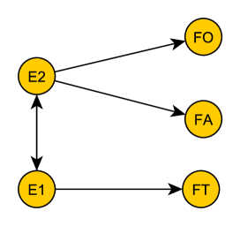
Figure 6: Mixed-chain graph for soft-drinks data

The MHMM with the lowest AIC value is also the most parsimonious model (last row in Table 1) which corresponds to the mixed-chain graph illustrated in Figure 6. It encodes the properties of double Granger noncausality and invariant association for the latent component of the MHMM, the local independence and the specific dependence of the observable variables on the latent chains for the observable component of the MHMM.

The second data set, available at $http://archive.ics.uci.edu/ml/$, reports daily measurements (from December 2006 to November 2010) of electric power consumption in one household. The energy (in watt-hour of active energy) from the sub-meter 1 corresponds to the kitchen, containing mainly a dishwasher, an oven and a microwave; the energy from the sub-meter 2 is used for the laundry room, containing a washing-machine, a tumble-drier, a refrigerator and a light; energy from sub-meter 3 corresponds to an electric water-heater and an air-conditioner. Here, the energy consumptions registered over 4 years by the sub-meters 1, 2, and 3, are categorized in low and high levels according to whether the real measurements are under or over an established threshold, and ${\bf F}_{1}$, ${\bf F}_{2}$ and ${\bf F}_{3}$ indicate the resulting categorical time series.

The categorized consumptions for kitchen, laundry and heater are the manifest variables used as indicators of the true need of energy for eating, cleaning and heating/cooling which is unobservable directly. The latent real request of energy, in fact, can be lower (higher) than the measured level due, for example, to waste (saving need). Therefore, we model the energy data through an MHMM involving three latent variables with two states and three observable binary variables.

Several hypotheses has been considered to describe the relations among the observable series and the latent factors, but in the sequel we will focus only on those models which better perform in terms of interpretability, parsimony and fitting.

Let us start by considering the saturated MHMM, i.e. without any restrictions, which attains $AIC=5493.015$, $loglike=-2634.507$, $par=112$.

Among the alternatives to the saturated model, a simple and intuitive linked MHMM considers that each of the three observable series of energy consumptions is an indicator of its specific latent variable and the observable variables are locally independent. Regarding the latent model, the three unobservable variables affect each others at the same time but each one depends only on the proper past (no Granger causality and no contemporaneous independence). This linked MHMM ($AIC=5621.251$, $loglike=-2778.626$, $par=32$) cannot be preferred to the saturated model. Also the coupled MHMM with every observable variable depending on its own latent variable and with contemporaneous independence and Granger causality among the three latent variables ($AIC=5615.272$, $loglike=-2777.636$, $par=30$) is outperformed by the saturated model.

Unfortunately, although combined with other different hypotheses on the latent component of the MHMM, the model restricted under the assumption of a specific effect of each latent variable on one and only one energy consumption series shows an unsatisfactory performance with an higher AIC value than that of the saturated model.

In the following models, the effects of two or more latent variables on the same observable variable will be considered additive as described in the expression (13).

An interesting model with a better fit assumes that: there is a specific effect of one latent variable on the energy consumptions for kitchen and laundry, another latent variable influences the energy consumptions for the heater, and there is a generic effect since a third latent variable affects all the manifest variables. This observation model is combined with the assumption that Granger causality and contemporaneous independence exist among all the latent variables. The model with these restrictions has $AIC=5470.029$, $loglike=-2702.014$, $par=33$. Its corresponding mixed-chain graph is reported in Figure 7 on the left.

The MHMM which seems the most suitable for representing the dynamics of the energy consumptions, among several models we fitted, assumes that: the first two latent variables are G-caused reciprocally, the third one depends only on its past, and there is contemporaneous independence among the three latent factors; moreover, there is local independence among the consumptions of the energy for eating, cleaning and air-conditioning which seem to depend on all the three latent variables ($AIC=5459.77$, $loglike=-2707.883$, $par=22$). Its mixed-chain graph is reported in Figure 7 on the right. This model is nested in an MHMM which shows a similar fit but admits that there is Granger causality among all the latent variables, the other hypotheses being equal ($AIC=5467.374$, $loglike=-2697.687$, $par=36$). When the two models are compared, the LRT ($LRT=20.4,df=14,p-value=0.118$) confirms that the most parsimonious model can be retained coherently with the AIC results.

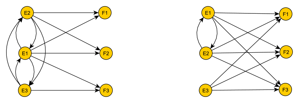
Figure 7: Mixed-chain graphs for energy data

References

- [1] Bartolucci, F., Colombi, R. and Forcina, A. (2007). An extended class of marginal link functions for modelling contingency tables by equality and inequality constraints. Statistica Sinica, 17, 691 – 711.
- [2] Bergsma, W. P. and Rudas, T. (2002). Marginal models for categorical data. The Annals of Statistics, 30, 140 – 159.
- [3] Brand, M., Oliver, N. and Pentland, A. (1997). Coupled hidden Markov models for complex action recognition. Proceedings of IEEE Computer Society Conference on Computer Vision and Pattern Recognition, 994 – 999.
- [4] Cappé, O., Moulines, E. and Rydén T. (2005). Inference in Hidden Markov Models. New York: Springer.
- [5] Ching, W.K., Fung, E.S. and Ng, M.K.(2002). A multivariate Markov chain for categorical data sequences and its applications in demand predictions. IMA J. Manag. Math., 13, 187 – 199.
- [6] Colombi, R. and Giordano, S. (2011). Testing lumpability for marginal discrete hidden Markov models. Advances in Statistical Analysis, 95, 293 – 311.
- [7] Colombi, R. and Giordano, S. (2012). Graphical models for multivariate Markov chains. Journal of Multivariate Analysis, 107, 90 – 103.
- [8] Colombi, R., Giordano, S. and Cazzaro, M. (2012). R-package hmmm: Hierarchical Multinomial Marginal Models. http://CRAN.R-project.org/package=hmmm.
- [9] Drton, M. (2009). Discrete chain graph models. Bernoulli, 15(3), 736 – 753.
- [10] Florens, J.P., Mouchart, M. and Rolin, J.M. (1993). Noncausality and marginalization of Markov processes. Econometric Theory, 9, 241 – 262.
- [11] Glonek, G.J.N. and McCullagh, P. (1995). Multivariate logistic models. Jornal of the Royal Statistical Society, Ser. B Stat. Methodol., 57, 533 – 546.
- [12] Koski, T. (2001). Hidden Markov Models for Bioinformatics. London: Kluwer Academic Publishers.
- [13] MacDonald, I.L. and Zucchini, W. (1997). Hidden Markov and Other Models for Discrete-valued Time Series. London: Chapman & Hall.
- [14] MacDonald, I.L. and Zucchini, W. (2009). Hidden Markov Models for Time Series, An introdution using R. London: Chapman & Hall.
- [15] Marchetti, G.M. and Lupparelli, M. (2011). Chain graph models of multivariate regression type for categorical data. Bernoulli, 17(3), 827 – 844.
- [16] Richardson, T. (2003). Markov properties for acyclic directed mixed graphs. Scandinavian Journal of Statistics, 30, 145 – 157.
- [17] Zucchini, W. and Guttorp, P. (1991). A hidden Markov model for space-time precipitation. Water Resourses Research, 27(8), 1917 – 1923.