Single-site-resolved measurement of the current statistics in optical lattices

Abstract

At present, great effort is spent on the experimental realization of gauge fields for quantum many-body systems in optical lattices. At the same time, the single-site-resolved detection of individual atoms has become a new powerful experimental tool. We discuss a protocol for the single-site resolved measurement of the current statistics of quantum many-body systems, which makes use of a bichromatic optical superlattice and single-site detection. We illustrate the protocol by a numerical study of the current statistics for interacting bosons in one and two dimensions and discuss the role of the on-site interactions for the current pattern and the ground-state symmetry for small two-dimensional lattices with artificial magnetic fields.

Introduction.—Improved and new detection techniques have contributed significantly to the rapid progress in the study of strongly correlated states of ultracold atoms in optical lattices in recent years. The combination of a time-of-flight expansion followed by absorption imaging gives access to the momentum distribution and has revealed the superfluid to Mott insulator transition (Greiner et al., 2002). Going further, one can study the noise correlations in these absorption images, e.g., exhibiting the quantum statistics of bosons (Fölling et al., 2005) and fermions (Rom et al., 2006). In addition, the excitation spectrum of interacting bosons has been measured using momentum-resolved Bragg spectroscopy (Ernst et al., 2010). However, the most significant step in recent times has arguably been the introduction of single-site detection (using fluorescence microscopy) in optical lattices (Bakr et al., 2009; Sherson et al., 2010). This new method has been used to observe the shell structure of a Mott insulator (Bakr et al., 2010; Sherson et al., 2010), the propagation of single bosons (Weitenberg et al., 2011), a spin impurity (Fukuhara et al., 2013), and the structure of density correlations (Endres et al., 2011). In the future, it may provide new insights into the buildup of entanglement in many-body systems and the influence of measurements on quantum many-body dynamics (Daley et al., 2012; Keßler et al., 2013, 2012).

Here, we discuss a scheme for the spatially resolved measurement of the current between nearest-neighbor lattice sites. It relies on combining a bichromatic superlattice and single-site detection. Such a tool is especially timely in the context of the recent effort towards realizing gauge fields in optical lattices (for recent reviews, see (Dalibard et al., 2011; Lewenstein et al., 2012; Goldman et al., 2013)), with first implementations reported in (Aidelsburger et al., 2011; Struck et al., 2012; Jiménez-García et al., 2012; Aidelsburger et al., 2013; Miyake et al., 2013). These systems can be used to realize states that support equilibrium currents. Various methods have by now been proposed to detect interesting aspects of such systems, e.g., quantum Hall edge states and Chern numbers in topological insulators, using time-of-flight expansion (Scarola and Das Sarma, 2007; Alba et al., 2011; Zhao et al., 2011; Polak and Zaleski, 2013; Wang et al., 2013), light scattering (Douglas and Burnett, 2011; Goldman et al., 2012), or the time evolution of the real space density after a quench in the potential (Killi and Paramekanti, 2012; Killi et al., 2012; Goldman et al., 2013). The protocol discussed below has similarities with the latter approach. However, in addition to probing the current pattern (Killi and Paramekanti, 2012), it reveals the full spatially resolved current statistics of the quantum-many body state, from which correlation functions can be extracted.

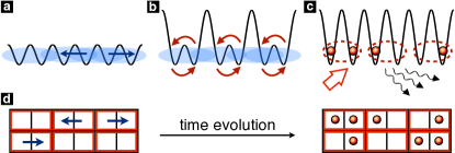
Fig. 1: (a)-(c) Protocol for measuring the current statistics of a quantum many-body state in an optical lattice. (b) An additional optical lattice with double wave length is suddenly ramped up [for a two-dimensional (2D) system, tunneling in the other direction is also turned off] and the on-site interaction between atoms is set close to zero. Afterwards, the atoms move within a double-well potential. (c) After some time, the motion is frozen out completely by also ramping up the barrier within each double well, and the atoms are detected by a single-site-resolved measurement. (d) An appropriate choice [see Eq. (3)] of the evolution time in the double-well potential (b) maps the current operator to the difference of the particle number at the right and left lattice site (shown for a 2D setup) and realizes a spatially resolved measurement of the current operator [Eq. (2)].

Model and current operator.—We consider a tight-binding Hamiltonian for ultracold atoms in an optical lattice,

$$\hat{\mathcal{H}}=-\sum_{<l,r>}\left\{J_{lr}\,\hat{c}_{l}^{\dagger}\hat{c}_{r}+J_{lr}^{*}\,\hat{c}_{r}^{\dagger}\hat{c}_{l}\right\}+\sum_{i}\epsilon_{i}\hat{n}_{i}+\hat{\mathcal{H}}_{int}.$$ (1)

Here, $\hat{c}_{l}^{(\dagger)}$ is a bosonic or fermionic annihilation (creation) operator, $J_{lr}$ is the possibly complex tunneling amplitude, and $<,>$ denotes pairs of nearest-neighbor lattice sites. The interaction part $\hat{\mathcal{H}}_{int}$ is a polynomial of local particle number operators, $\hat{n}_{i}=\hat{c}_{i}^{\dagger}\hat{c}_{i}$, and $\epsilon_{i}$ is the on-site energy at site $i$. The (mass) current operator for this system can be defined using the local continuity equation for the particle density. For a lattice system it reads $\frac{d}{dt}\hat{n}_{l}+\sum_{r\in\mathrm{NN}(l)}\,\hat{\jmath}_{l\rightarrow r}=0$, here $\hat{\jmath}_{l\rightarrow r}$ denotes the current from site $l$ to site $r$ and $\mathrm{{NN}}(l)$ denotes the set of nearest-neighbor lattice sites of $l.$ Using Heisenberg’s equation of motion gives $\frac{d}{dt}\hat{n}_{l}=i\sum_{r\in\mathrm{NN}(l)}\{J_{lr}\,\hat{c}_{l}^{\dagger}\hat{c}_{r}-J_{lr}^{*}\,\hat{c}_{r}^{\dagger}\hat{c}_{l}\}$, and accordingly the current operator between nearest-neighbor lattice sites $l$ and $r$ reads (for bosons and fermions)

$$\hat{\jmath}_{l\rightarrow r}=-i\left\{J_{lr}\,\hat{c}_{l}^{\dagger}\hat{c}_{r}-J_{lr}^{*}\,\hat{c}_{r}^{\dagger}\hat{c}_{l}\right\}.$$ (2)

Measurement protocol.—The protocol for measuring the eigenvalues of the current operator (2) is summarized in Fig. 1. The main idea is to use a bichromatic superlattice, which has already been realized experimentally (Sebby-Strabley et al., 2006; Trotzky et al., 2010), and to apply a beam-splitter operation to map the single-particle eigenstates of the current operator to the states localized at the left and right lattice site of each double well [Fig. 1(b)]. The measured value of the current operator is then essentially given by the difference of the particle numbers of both lattice sites. The particle number can be measured [Figs. 1(c) and 1(d)] in principle by the recently developed single-site imaging techniques (Bakr et al., 2009; Sherson et al., 2010), although at present these are still restricted to parity measurements (see the discussion on experimental details below).

Formally, the protocol relies on the time evolution of noninteracting atoms in a symmetric double-well potential, $\hat{\mathcal{H}}=-(J_{lr}\hat{c}_{l}^{\dagger}\hat{c}_{r}+J_{lr}^{*}\hat{c}_{r}^{\dagger}\hat{c}_{l}).$ The difference in the atom number at the two wells oscillates in time and can be expressed as

$$\hat{n}_{r}(t)-\hat{n}_{l}(t)=\cos(2Jt)[\hat{n}_{r}(0)-\hat{n}_{l}(0)]+\sin(2Jt)\frac{\hat{\jmath}_{l\rightarrow r}(0)}{J},$$ (3)

where $J=|J_{lr}|.$ Thus, the current can be obtained as the density difference, $\hat{\jmath}_{l\rightarrow r}(0)=(-1)^{m}J\left[\hat{n}_{r}(\tilde{t})-\hat{n}_{l}(\tilde{t})\right]$, for suitable chosen evolution times $J\tilde{t}=\pi(2m+1)/4$, $m\in\mathbb{{N}}_{0}$.

The previous expression for $\hat{\jmath}_{l\rightarrow r}(0)$ shows that the current operator has discrete eigenvalues, just like the particle number operator. This situation, surprising at first sight, can also be understood as follows: The eigenvalues of the current operator are given by the difference in the density of atoms going to the right and left times the velocity. This is seen by diagonalizing the current operator (2), which yields $\hat{\jmath}_{l\rightarrow r}=J(\hat{c}_{\rightarrow}^{\dagger}\hat{c}_{\rightarrow}-\hat{c}_{\leftarrow}^{\dagger}\hat{c}_{\leftarrow})$ with $\hat{c}_{\rightarrow}=(\hat{c}_{r}+iJ_{lr}^{*}\hat{c}_{l}/J)/\sqrt{2}$ and $\hat{c}_{\leftarrow}=(\hat{c}_{r}-iJ_{lr}^{*}\hat{c}_{l}/J)/\sqrt{2}$. The operators $\hat{c}_{\rightarrow}$ and $\hat{c}_{\leftarrow}$ have a simple meaning: They correspond to right- and left-going atoms (Foo, ). Since the total particle number in the double well, $\hat{n}_{l}+\hat{n}_{r}$, commutes with $\hat{\jmath}_{l\rightarrow r}$, we can assume a situation of fixed $n_{l}+n_{r}$. Then the spectrum of the current operator is $J\cdot\{-n,-n+2,\ldots,n\}$, with $n=n_{l}+n_{r}$ for bosons and $n=[n_{l}+n_{r}]\,\mbox{mod}\,2$ for fermions due to the Pauli principle.

Bosons in 1D.—We first consider the current statistics of the homogeneous one-dimensional (1D) Bose-Hubbard model,

$$\hat{\mathcal{H}}=-J\sum_{i}\left\{\hat{c}_{i+1}^{\dagger}\hat{c}_{i}+\hat{c}_{i}^{\dagger}\hat{c}_{i+1}\right\}+\frac{U}{2}\sum_{i}\hat{n}_{i}(\hat{n}_{i}-1),$$ (4)

with real tunneling amplitude $J$ and on-site interaction strength $U$. To keep the numerics manageable, we focus on the 1D case, even though we believe that the qualitative features of the local properties we are going to discuss should not be dependent on dimensionality in a significant way. The two phases of the Bose-Hubbard model exhibit a characteristic atom number statistics at a single site: a Poisson distribution for the superfluid state ($U/J\rightarrow 0$) and a fixed atom number in the Mott insulating regime ($U/J\rightarrow\infty$) for integer filling $\bar{n}$; see, e.g., Refs. (Jaksch et al., 1998; Bloch et al., 2008).

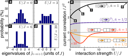
Fig. 2: Current statistics for the ground state of interacting bosons in a 1D lattice. The results are obtained by exact diagonalization of a lattice with 12 or 16 sites for filling $\bar{n}=1$ and $\bar{n}=1/2$, respectively, and periodic boundary conditions. (a)-(d) Distribution of the current eigenvalues for $\bar{n}=1$ and interaction strength $U/J=0,3,6,20$ [(a)-(d)] calculated from 25000 snapshots. The vanishing mean current $\langle\hat{\jmath}_{i\rightarrow i+1}\rangle$ is reflected by the $j\mapsto-j$ symmetry of the distributions. (e) Interaction dependence of the variance of the current, $\langle(\hat{\jmath}_{i\rightarrow i+1})^{2}\rangle$, and the current-current correlation $\langle\hat{\jmath}_{i\rightarrow i+1}\hat{\jmath}_{i+2\rightarrow i+3}\rangle$ for unit filling and half filling. The variance of the current increases monotonically with $U/J$ in both cases. Interestingly, extremal values of the current-current correlation show up at intermediate interaction strengths for $\bar{n}=1$.

The corresponding current statistics is presented in Figs. 2(a)-2(d) at filling $\bar{n}=1$. For $U=0$, the atoms are in a product state of coherent states at the individual sites. Thus, $n_{\rightarrow}$ and $n_{\leftarrow}$ are also Poisson distributed, with mean $\bar{n}$. The current (2), being the difference between two Poisson distributed variables, is then given by the so-called Skellam distribution, $P_{\bar{n}}(j=Jm)=e^{-2\bar{n}}\mathcal{I}_{|m|}(2\bar{n})$, where $\mathcal{I}$ denotes the modified Bessel function. When increasing $U/J$, the distribution becomes more and more concentrated at the eigenvalues $\pm 2J.$ This is a consequence of the Mott insulating state being a superposition of the eigenstates corresponding to $j=\pm 2J$, $\hat{c}_{i}^{\dagger}\hat{c}_{i+1}^{\dagger}\ket{\mbox{vac}}=\frac{1}{2}[(\hat{c}_{\rightarrow}^{\dagger})^{2}-(\hat{c}_{\leftarrow}^{\dagger})^{2}]\ket{\mbox{vac}}$. Note that, in general, the current eigenvalues are even multiples of $J$ for the Mott insulator at arbitrary integer filling.

Figure 2(e) shows the interaction dependence of current correlation functions, which might be detected using the scheme proposed here. The variance of the current increases monotonically with the on-site interaction strength, from $\langle\hat{\jmath}_{i\rightarrow i+1}^{2}\rangle_{SF}=2J^{2}\bar{n}$ for $U=0$ to $\langle\hat{\jmath}_{i\rightarrow i+1}^{2}\rangle_{MI}=2J^{2}\bar{n}(\bar{n}+1)$ at integer filling $\bar{n}$ deep in the Mott insulating regime. For $\bar{n}=1,$ the current correlation between neighboring pairs of lattice sites, $\langle\hat{\jmath}_{i\rightarrow i+1}\hat{\jmath}_{i+2\rightarrow i+3}\rangle$, becomes negative for intermediate $U/J$ with a minimum close to the superfluid-to-Mott-insulator transition, while it vanishes for $U\rightarrow 0$ and $U/J\rightarrow\infty$. In contrast, for a half-filled lattice, $\langle\hat{\jmath}_{i\rightarrow i+1}\hat{\jmath}_{i+2\rightarrow i+3}\rangle$ decreases asymptotically as one goes into the hardcore boson limit ($U/J\rightarrow\infty$).

We note that the correlations of the current into and through a lattice site might be accessed by an extended version of the measurement scheme using a triple well-superlattice structure; see Supplemental Material (Sup, ).

Bosons in a synthetic magnetic field.—We consider interacting bosons subject to a uniform synthetic magnetic field perpendicular to the 2D lattice. The corresponding Hamiltonian reads, in Landau gauge,

$$\hat{\mathcal{H}} = -J\sum_{x,y}\left\{\hat{c}_{x+1,y}^{\dagger}\hat{c}_{x,y}+\hat{c}_{x,y+1}^{\dagger}\hat{c}_{x,y}e^{i2\pi\alpha x}+\mbox{h.c.}\right\}$$ (5)

$$+\frac{U}{2}\sum_{x,y}\hat{n}_{x,y}(\hat{n}_{x,y}-1).$$

Here, $x,y$ are the integer $x$ and $y$ coordinates of the lattice sites, and the phase $2\pi\alpha$, which a boson picks up when circulating in an anticlockwise direction around a unit cell, encodes the effect of the magnetic field. For a charged particle, $\alpha$ would equal the number of flux quanta per unit cell. The single-particle spectrum of (5) is given by the famous fractal “Hofstadter butterfly” (Hofstadter, 1976).

Below we discuss relatively small 2D lattices, which might be realized first in experiments (with a suitable superlattice structure dividing the entire lattice into such small plaquettes as implemented for $2\times 2$ lattices in (Aidelsburger et al., 2011)). A similar system has been realized with Bose-Einstein condensates in rotating lattices (Tung et al., 2006; Williams et al., 2010), where the “Lorentz force” is replaced by the Coriolis force (Cooper, 2008). The creation and observation of topological states in this setup have been theoretically studied in (Barberán et al., 2006; Hafezi et al., 2007; Palmer et al., 2008; Umucalilar et al., 2008; Umucalilar and Mueller, 2010; Graß et al., 2012). Moreover, a transition between ground states of different rotational symmetry at discrete rotation frequencies was found (Bhat et al., 2006, 2006), which leads to a discontinuity in the edge current. Here, we study the effects of finite on-site interactions on such transitions (these previous works (Bhat et al., 2006, 2006) discussed only the limit of hardcore bosons).

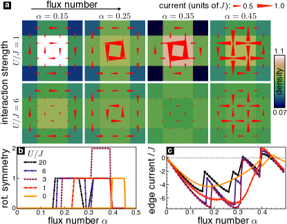
Fig. 3: Ground-state properties of nine interacting bosons in a $4\times 4$ lattice with artificial magnetic field (similar behavior is found for different fillings): (a) current and density pattern, (b) rotational symmetry, and (c) edge current. Increasing the flux number starting from $\alpha=0$, the current flows in clockwise directions and grows with $\alpha$. The current in the center is generally suppressed for larger $U/J$, and it reverses its direction above a certain critical value of $\alpha$ (which decreases with increasing $U/J$). This change appears together with (b) a transition in the rotational symmetry of the ground state and (c) a discontinuity in the edge current. Large interactions lead to additional configurations, as shown, e.g., in the panel for $U/J=6$ and $\alpha=0.35$.

The results obtained from exact diagonalization for a $4\times 4$ lattice are summarized in Fig. 3. Note that we restrict ourselves to the interval $\alpha\in[0,0.5]$, as the Hamiltonian is invariant under $\alpha\mapsto\alpha+1$, and $\alpha\mapsto-\alpha$ only changes the magnetic field direction. Figure 3(a) shows the current and density profile of the ground state for different interaction strengths and $\alpha$’s. The current patterns found for $U/J=1$ are similar to those of $U/J=0$ (not shown), whereas additional current configurations appear for large $U/J$. Note that the central current reverses sign beyond some critical flux number $\alpha$, and this value decreases for larger $U/J$.

The critical value of $\alpha$ can be identified via the change in the ground-state rotational symmetry or via the first discontinuity of the edge current. We define the edge current as the sum of all currents along the boundary, counted in an anticlockwise direction; see Fig. 3(c). The rotational symmetry is best discussed in the symmetric gauge; see (Sup, ). For a square lattice, the Hamiltonian (5) commutes with the rotation by $\pi/2$, $\mathcal{R}(\pi/2)$. Thus, a nondegenerate ground state is an eigenstate of $\mathcal{R}(\pi/2)$, with eigenvalue $e^{i\pi m/2}$, $m=0,1,2,3$. Additional transitions in the ground-state symmetry (discontinuities of the edge current) show up for intermediate $U/J$. The critical flux numbers for these transition points hardly change for $U/J\apprge 10$. The discussed current patterns and the edge current can be measured using the proposed protocol, which therefore provides a means of studying the flux and interaction dependence of such transitions.

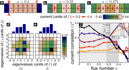
Fig. 4: Current statistics of the ground state of interacting bosons in a $8\times 2$ lattice at half filling, calculated from 25000 snapshots. (a)-(c) Density and current profile for interaction strength $U/J=8$ and different flux numbers $\alpha$. (d),(e) Joint eigenvalue distribution for different current operators and the parameters used in (a). Note that the currents at the links A,B, and C are defined in the positive $x$ direction. While $\hat{\jmath}_{B}$ and $\hat{\jmath}_{C}$ have the same eigenvalue distribution (see histograms), their joint distribution with $\hat{\jmath}_{A}$ is different: $\hat{\jmath}_{A}$ and $\hat{\jmath}_{C}$ are uncorrelated, but $\hat{\jmath}_{A}$ and $\hat{\jmath}_{B}$ are correlated. (f) Current correlation $\langle\hat{\jmath}_{A}\hat{\jmath}_{B}\rangle-\langle\hat{\jmath}_{A}\rangle\langle\hat{\jmath}_{B}\rangle$ for different interaction strengths ($U/J=0.5,2,4,8,25$, bright to dark). Surprisingly, large on-site interactions lead to a strong positive current correlation for flux numbers corresponding to the current pattern (a). The inset shows the $\alpha$ dependence of the mean current $\langle\hat{\jmath}_{B}\rangle$ for the same interaction strengths (note that $\langle\hat{\jmath}_{A}\rangle=-\langle\hat{\jmath}_{B}\rangle$).

We now turn to spatial current correlations. An illustrative example is displayed in Fig. 4, for a half-filled $8\times 2$ lattice. Such bosonic flux ladders exhibit a transition from a Meißner phase [Fig. 4(a)] to a vortex phase [Fig. 4(b)] when $\alpha$ is increased (Orignac and Giamarchi, 2001; Cha and Shin, 2011). For the situation shown in Fig. 4(a), we address the question of whether the currents at A, B, and C are correlated. This is done by constructing the joint probability distribution of the eigenvalues from an ensemble of snapshots, since the currents $\hat{\jmath}_{A},\,\hat{\jmath}_{B},$ and $\hat{\jmath}_{C}$ can be measured simultaneously. Figures 4(d) and 4(e) display two examples of these joint probability distributions. The measured values of $\hat{\jmath}_{A}$ and $\hat{\jmath}_{C}$ at the two far-removed links A and C are (to a very good approximation) independent of each other, i.e., the joint probability distribution is just a product of the eigenvalue distribution of $\hat{\jmath}_{A}$ and $\hat{\jmath}_{C}$ [cf. Fig. 4(e)]. In contrast, the current operators $\hat{\jmath}_{A}$ and $\hat{\jmath}_{B}$ for nearby sites are correlated as the joint probabilities $p(j_{A}=-J,j_{B}=-J)$ and $p(j_{A}=-J,j_{B}=0)$ are clearly different even though $p(j_{B}=-J)$ and $p(j_{B}=0)$ are almost equal; see Fig. 4(d). The dependence of the current correlation $\langle\hat{\jmath}_{A}\hat{\jmath}_{B}\rangle-\langle\hat{\jmath}_{A}\rangle\langle\hat{\jmath}_{B}\rangle$ on the flux number $\alpha$ is shown in Fig. 4(f). We find a positive correlation for $\alpha\apprle 0.3$ [parameter regime with the current pattern shown in Fig. 4(a)], which becomes stronger with increasing on-site interaction strength. In contrast, the average current [inset in Fig. 4(f)] hardly changes with the interaction strength for $U/J\gtrsim 2$. For larger flux values, the correlation falls off to values around zero.

Discussion of experimental details.—Let us consider the combination of the proposed measurement protocol with gauge fields created by laser-assisted tunneling (Jaksch and Zoller, 2003; Gerbier and Dalibard, 2010; Kolovsky, 2011) implemented in (Aidelsburger et al., 2011, 2013; Miyake et al., 2013). The required 2D lattice consists of alternating columns with different on-site energies (and may trap different internal states (Jaksch and Zoller, 2003; Gerbier and Dalibard, 2010)). Tunneling between different columns is only nonzero when it is driven by additional light fields (which also imprint the phase on the tunneling amplitude), while bare tunneling exists within each column. Thus, the bichromatic superlattice for the current measurement could be applied in the direction of the columns, while the tunneling between the columns is inhibited by switching off the driving laser fields.

All of the present experiments on single-site-resolved detection only resolve the parity of the atom number at any lattice site (Bakr et al., 2009; Sherson et al., 2010). For a single or two coupled 1D chains, considered in Figs. 2 and 4, one might let the atoms expand into another direction before the detection process (similar to (Weitenberg et al., 2011)) to avoid double or higher occupancies. However, for true 2D configurations, one is currently restricted to small filling factors, until the parity problem can be circumvented via alternative approaches. We have further investigated these limitations of the measurement protocol for the configuration shown in Fig. 4, by numerically simulating situations with parity detection only. We also included residual interactions, $U_{res}$, and timing errors during the evolution in the double-well potential. We find that the current pattern and the current correlation can still be observed in the presence of parity detection, even though the absolute value of the observed current decreases by up to 25%. The influence of the residual interaction is of the order of a few percent for $U_{res}/J\leq 1/4$. A timing error $J\tilde{t}=\pi/4+J\Delta t$ leads to a change in the current and current correlation of less than $0.02J$ and $0.01J^{2}$, respectively, for $J\Delta t\leq 0.05$.

Conclusions.—We have analyzed a protocol for the site-resolved measurement of the current operator in optical lattices. Using already available experimental techniques, it can be employed for interacting bosons at small filling factors. It can, in principle, be extended to fermions and possibly also to situations with different species. Measuring the statistics and spatial structure of currents seems a promising tool to study the physics of interacting ultracold atoms subject to gauge fields.

Acknowledgments.—We thank the DFG for support in the Emmy-Noether programme and the SFB/TR 12.

Note added.—The Meißner phase in a bosonic flux ladder [cf. Fig. 4(a)] was recently observed experimentally by measuring the average edge currents (Atala et al., 2014).

Supplemental Material for “Single-site-resolved measurement of the current statistics in optical lattices”

Stefan Keßler¹ and Florian Marquardt^1,2

¹Institute for Theoretical Physics, Universität Erlangen-Nürnberg, Staudtstraße 7, 91058 Erlangen, Germany
²Max Planck Institute for the Science of Light, Günther-Scharowsky-Straße 1/Bau 24, 91058 Erlangen, Germany

I Extended Measurement scheme

In the main text we describe a projective measurement of the current operator between two nearest-neighbor lattice sites. From the measurement outcomes one can calculate the expectation values of any sum of current operators of the form (2), as, for instance, the edge current. Here, we discuss an extended setup with the double-well potential replaced by a triple-well potential [cf. Fig. 1(b)]. This modification allows to measure the statistics of the (one-dimensional) current through a lattice site, $\hat{\jmath}_{i-1\rightarrow i}+\hat{\jmath}_{i\rightarrow i+1}$. The obtained statistics can be used (together with the one of the “usual” setup) to evaluate, e.g., the variance of the (one-dimensional) current into a lattice site, $\hat{\jmath}_{i-1\rightarrow i}-\hat{\jmath}_{i\rightarrow i+1}$. This variance cannot be conceived from the statistics of $\hat{\jmath}_{i\rightarrow i+1}$ alone as it involves the expectation value $\langle\hat{\jmath}_{i-1\rightarrow i}\hat{\jmath}_{i\rightarrow i+1}\rangle$.

We assume a laser configuration, which allows to create a triple-well superlattice structure in one spatial direction, such that the dynamics within each triple well is described by $\hat{\mathcal{H}}^{(3)}=-J\sum_{l=1}^{2}(\hat{c}_{l}^{\dagger}\hat{c}_{l+1}+\hat{c}_{l+1}^{\dagger}\hat{c}_{l})$. We restrict to the case of a real tunneling amplitude $J$ assuming the superlattice to be applied in the direction of the columns, where no phase is imprinted on the tunneling amplitude (see discussion of experimental details in the main text). Experimentally, the triple-well superlattice might be realized by the use of a bichromatic lattice with an additional laser beam with half the wavelength of the short lattice, as discussed in (Schlagheck et al., 2010). The diagonalization of the three-site Hamiltonian yields $\hat{\mathcal{H}}^{(3)}=-2J\sum_{n=1}^{3}\cos(\frac{\pi n}{4})\hat{d}_{n}^{\dagger}\hat{d}_{n}$ with $\hat{d}_{n}=\sum_{l=1}^{3}(U^{\dagger})_{nl}\hat{c}_{l}$ and $U_{ln}=\frac{1}{\sqrt{2}}\sin(\frac{\pi ln}{4})$. Making use of the expression for the time-dependent annihilation operator, $\hat{c}_{l}(t)=\sum_{n,s=1}^{3}U_{ln}\exp\{i2J\cos(\frac{n\pi}{4})t\}[U^{\dagger}]_{ns}\hat{c}_{s}(0)$, the current through lattice site 2, $\hat{\jmath}_{1\rightarrow 2}+\hat{\jmath}_{2\rightarrow 3}$, at time zero (ramp up of the triple-well potential) expressed in terms of the one-particle density matrix after an evolution time $t$ equals

$$\hat{\jmath}_{1\rightarrow 2}(0)+\hat{\jmath}_{2\rightarrow 3}(0)=J\sum_{l,n=1}^{3}\hat{c}_{l}^{\dagger}(t)A_{ln}\hat{c}_{n}(t),$$ (S.1)

with

$$A=\left[\begin{array}[]{ccc}-\sqrt{2}\sin(\sqrt{2}Jt)&-i\cos(\sqrt{2}Jt)&0\\ i\cos(\sqrt{2}Jt)&0&-i\cos(\sqrt{2}Jt)\\ 0&i\cos(\sqrt{2}Jt)&\sqrt{2}\sin(\sqrt{2}Jt)\end{array}\right].$$ (S.2)

At time points $J\tilde{t}=\pi(m+\frac{1}{2})/\sqrt{2}$, $m\in\mathbb{{N}}_{0}$, only the diagonal terms of the one-particle density matrix contribute and the current is given by

$$\hat{\jmath}_{1\rightarrow 2}(0)+\hat{\jmath}_{2\rightarrow 3}(0)=(-1)^{m}\sqrt{2}J[\hat{n}_{3}(\tilde{t})-\hat{n}_{1}(\tilde{t})].$$ (S.3)

The density difference on the right-hand side can be measured by a single-site-resolved measurement of the atom number. The meaning of Eq. (S.3) is rather simple: For the time span $J\tilde{t}=\pi/(2\sqrt{2})$ the single-particle eigenstates corresponding to the current eigenvalues $-\sqrt{2}J,$ 0, and $\sqrt{2}J$ are mapped on the states localized at the lattice sites 1,2, and 3, respectively. Note that a symmetric triple-well potential cannot be used for the direct detection of the current into lattice site 2, $\hat{\jmath}_{1\rightarrow 2}(0)-\hat{\jmath}_{2\rightarrow 3}(0)$, as this current operator and three-site Hamiltonian have the common eigenstate $\frac{1}{\sqrt{2}}(\hat{c}_{3}^{\dagger}-\hat{c}_{1}^{\dagger})\ket{\mbox{vac}}.$ Therefore, there is never a time for which this difference of current operators can be expressed as a combination of single-site densities.

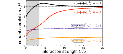
Fig. S1: Variance of the current through and into a lattice site $\langle(\hat{\jmath}_{i-1\rightarrow i}+\hat{\jmath}_{i\rightarrow i+1})^{2}\rangle$ and $\langle(\hat{\jmath}_{i-1\rightarrow i}-\hat{\jmath}_{i\rightarrow i+1})^{2}\rangle$, respectively, for the ground state of interacting bosons in a 1D lattice. The parameters are the same as in Fig. 2. For integer filling $\bar{n}$, the variances of both currents approach each other deep in the Mott insulating regime, whereas the fluctuation in the current into a lattice site is much larger than the fluctuation in the current through a lattice site for small on-site interaction strength $U.$

Figure S1 presents the variance of the current through and into a lattice site for the 1D Bose-Hubbard model, which is also considered in the main text. The mean value of both currents vanishes for the ground state since $\langle\hat{\jmath}_{i\rightarrow i+1}\rangle=0$; see also Figs. 2(a-d). Figure S1 shows a drastic interaction dependence for a lattice with integer filling $\bar{n}.$ For the superfluid state, the fluctuation of the current into a lattice site, and thus $\langle(\frac{d}{dt}\hat{n}_{i})^{2}\rangle$, is much stronger than the fluctuation of the current through a lattice site. In contrast, they are the same in the Mott insulating regime in the limit $U/J\rightarrow\infty$.

II Rotational symmetry

Here, we discuss the ground-state rotational symmetry for a many-body system described by Hamiltonian (5); see also (Bhat et al., 2006). We consider a square lattice of $N\times N$ lattice sites [for a rectangular lattice the following reasoning is essentially the same replacing $\hat{R}(\pi/2)$ by $\hat{R}(\pi)$, which results in two eigenvalues $m=0,1$]. An anticlockwise rotation of the coordinate system (passive rotation) by an angle $\pi/2$ maps the lattice sites onto themselves, $\hat{R}(\pi/2)\ket{x,y}=\ket{y,-x}$, with the $x$ and $y$ components $x,y\in\{-\frac{N-1}{2},-\frac{N-1}{2}+1,\ldots,\frac{N-1}{2}\}.$ Applying $\hat{R}(\pi/2)$ four times is equivalent to the identity transformation and thus the possible eigenvalues of $\hat{R}(\pi/2)$ are given by the fourth roots of one, $\lambda_{m}=\exp\{i2\pi m/4\}$ with $m=0,1,2,3.$

Let us now consider the Hamiltonian (5) for this square lattice. It reads in the symmetric gauge [in Eq. (5) we used the Landau gauge], which identifies the center-of-mass of the lattice as a special point:

$$\hat{\mathcal{H}} = -J\sum_{y;x\neq(N-1)/2}\left\{\hat{c}_{x+1,y}^{\dagger}\hat{c}_{x,y}e^{-i\pi\alpha y}+\mbox{h.c.}\right\}$$ (S.4)

$$-J\sum_{x;y\neq(N-1)/2}\left\{\hat{c}_{x,y+1}^{\dagger}\hat{c}_{x,y}e^{i\pi\alpha x}+\mbox{h.c.}\right\}$$

$$+\frac{U}{2}\sum_{x,y}\hat{n}_{x,y}(\hat{n}_{x,y}-1).$$

The transformation of the annihilation (creation) operator under the rotation, $\hat{R}(\pi/2)\hat{c}_{x,y}^{(\dagger)}\hat{R}(\pi/2)^{T}=\hat{c}_{-y,x}^{(\dagger)}$, makes it directly apparent that this Hamiltonian commutes with $\hat{R}(\pi/2)$, i.e., $\hat{\mathcal{H}}=\hat{R}(\pi/2)\hat{\mathcal{H}}\hat{R}(\pi/2)^{T}$. Thus, for an eigenstate $\ket{\Psi_{i}}$ of $\hat{\mathcal{H}}$, $\hat{R}(\pi/2)\ket{\Psi_{i}}$ is also an eigenstate of $\hat{\mathcal{H}}$ with the same eigenvalue $E_{i}$. If $E_{i}$ is nondegenerate, then $\ket{\Psi_{i}}$ is an eigenstate of $\hat{R}(\pi/2)$, too.

In the main text, we discuss the rotational symmetry and the edge current of the ground state of Hamiltonian (5) as function of the parameters $\alpha$ and $U/J$. A change in the rotational symmetry of a (nondegenerate) ground state happens by an exact level crossing of the two lowest eigenenergies (as these states correspond to two different irreducible representations of the rotation; see (Landau and Lifshitz, 1977)). This implies that the ground-state energy is nonanalytic at the crossing point and we also observe a discontinuity in the edge current.

III Timing error

Let us discuss on more general grounds the effect of an imprecisely chosen evolution time in the double-well potential [Fig. 1(b)] on the current measurement. We consider an evolution time $J\tilde{t}=\pi/4+J\Delta t$, where $J\Delta t$ is the (dimensionless) timing error. The actually measured density difference between the left and the right well is given by Eq. (3) in the main text. For a small timing error $J\Delta t\ll 1,$ it yields up to second order in $(J\Delta t)^{2}$:

$$\hat{n}_{r}(\tilde{t})-\hat{n}_{l}(\tilde{t}) = [1-2(J\Delta t)^{2}]\,\hat{\jmath}_{l\rightarrow r}(0)/J$$

$$-2(J\Delta t)[\hat{n}_{r}(0)-\hat{n}_{l}(0)]+\mathcal{O}([J\Delta t]^{3}).$$

The comparison with the ideal case, $\hat{n}_{r}(\tilde{t})-\hat{n}_{l}(\tilde{t})=\hat{\jmath}_{l\rightarrow r}(0)/J$, shows that there are two contributions that lead to an error in the current measurement: one proportional to the true value of the current and another proportional to the initial density difference between the two lattice sites. The first term is just a relative change of the current by $2(J\Delta t)^{2}$, which should be very small in an experimental realization of the measurement protocol. The second term seems to be more severe since it is linear in the timing error $J\Delta t$ and does not depend on the value of the current. However, for the evaluation of the average current this error is suppressed for a system with an approximately homogeneous density distribution or in case that the distribution of timing errors over different measurement runs is roughly symmetric with respect to $J\Delta t=0.$ Indeed, we have found only a small effect of the timing error on the current and the current correlations for the results shown in Fig. 4 (as reported in the main text), where the density distribution is roughly homogeneous.

References

- Greiner et al. (2002) M. Greiner, O. Mandel, T. Esslinger, T. W. Hänsch, and I. Bloch, Nature 415, 39 (2002).
- Fölling et al. (2005) S. Fölling, F. Gerbier, A. Widera, O. Mandel, T. Gericke, and I. Bloch, Nature 434, 481 (2005).
- Rom et al. (2006) T. Rom, T. Best, D. van Oosten, U. Schneider, S. Fölling, B. Paredes, and I. Bloch, Nature 444, 733 (2006).
- Ernst et al. (2010) P. T. Ernst, S. Götze, J. S. Krauser, K. Pyka, D.-S. Lühmann, D. Pfannkuche, and K. Sengstock, Nature Physics 6, 56 (2010).
- Bakr et al. (2009) W. S. Bakr, J. I. Gillen, A. Peng, S. Fölling, and M. Greiner, Nature 462, 74 (2009).
- Sherson et al. (2010) J. F. Sherson, C. Weitenberg, M. Endres, M. Cheneau, I. Bloch, and S. Kuhr, Nature 467, 68 (2010).
- Bakr et al. (2010) W. S. Bakr, A. Peng, M. E. Tai, R. Ma, J. Simon, J. I. Gillen, S. Fölling, L. Pollet, and M. Greiner, Science 329, 547 (2010).
- Weitenberg et al. (2011) C. Weitenberg, M. Endres, J. F. Sherson, M. Cheneau, P. Schauß, T. Fukuhara, I. Bloch, and S. Kuhr, Nature 471, 319 (2011).
- Fukuhara et al. (2013) T. Fukuhara, A. Kantian, M. Endres, M. Cheneau, P. Schauß, S. Hild, D. Bellem, U. Schollwöck, T. Giamarchi, C. Gross, I. Bloch, and S. Kuhr, Nature Physics 9, 235 (2013).
- Endres et al. (2011) M. Endres, M. Cheneau, T. Fukuhara, C. Weitenberg, P. Schauß, C. Gross, L. Mazza, M. Bañuls, L. Pollet, I. Bloch, and S. Kuhr, Science 334, 200 (2011).
- Daley et al. (2012) A. J. Daley, H. Pichler, J. Schachenmayer, and P. Zoller, Phys. Rev. Lett. 109, 020505 (2012).
- Keßler et al. (2013) S. Keßler, I. P. McCulloch, and F. Marquardt, New Journal of Physics 15, 053043 (2013).
- Keßler et al. (2012) S. Keßler, A. Holzner, I. P. McCulloch, J. von Delft, and F. Marquardt, Phys. Rev. A 85, 011605(R) (2012).
- Dalibard et al. (2011) J. Dalibard, F. Gerbier, G. Juzeliūnas, and P. Öhberg, Rev. Mod. Phys. 83, 1523 (2011).
- Lewenstein et al. (2012) M. Lewenstein, A. Sanpera, and V. Ahufinger, Ultracold Atoms in Optical Lattices: Simulating Quantum Many-body Systems, 1st ed. (Oxford University Press, Oxford, 2012) ISBN 9780199573127.
- Goldman et al. (2013) N. Goldman, G. Juzeliūnas, P. Öhberg, and I. B. Spielman, arXiv:1308.6533 .
- Aidelsburger et al. (2011) M. Aidelsburger, M. Atala, S. Nascimbène, S. Trotzky, Y.-A. Chen, and I. Bloch, Phys. Rev. Lett. 107, 255301 (2011).
- Struck et al. (2012) J. Struck, C. Ölschläger, M. Weinberg, P. Hauke, J. Simonet, A. Eckardt, M. Lewenstein, K. Sengstock, and P. Windpassinger, Phys. Rev. Lett. 108, 225304 (2012).
- Jiménez-García et al. (2012) K. Jiménez-García, L. J. LeBlanc, R. A. Williams, M. C. Beeler, A. R. Perry, and I. B. Spielman, Phys. Rev. Lett. 108, 225303 (2012).
- Aidelsburger et al. (2013) M. Aidelsburger, M. Atala, M. Lohse, J. T. Barreiro, B. Paredes, and I. Bloch, Phys. Rev. Lett. 111, 185301 (2013a).
- Miyake et al. (2013) H. Miyake, G. A. Siviloglou, C. J. Kennedy, W. C. Burton, and W. Ketterle, Phys. Rev. Lett. 111, 185302 (2013).
- Scarola and Das Sarma (2007) V. W. Scarola and S. Das Sarma, Phys. Rev. Lett. 98, 210403 (2007).
- Alba et al. (2011) E. Alba, X. Fernandez-Gonzalvo, J. Mur-Petit, J. K. Pachos, and J. J. Garcia-Ripoll, Phys. Rev. Lett. 107, 235301 (2011).
- Zhao et al. (2011) E. Zhao, N. Bray-Ali, C. J. Williams, I. B. Spielman, and I. I. Satija, Phys. Rev. A 84, 063629 (2011).
- Polak and Zaleski (2013) T. P. Polak and T. A. Zaleski, Phys. Rev. A 87, 033614 (2013).
- Wang et al. (2013) L. Wang, A. A. Soluyanov, and M. Troyer, Phys. Rev. Lett. 110, 166802 (2013).
- Douglas and Burnett (2011) J. S. Douglas and K. Burnett, Phys. Rev. A 84, 053608 (2011).
- Goldman et al. (2012) N. Goldman, J. Beugnon, and F. Gerbier, Phys. Rev. Lett. 108, 255303 (2012).
- Killi and Paramekanti (2012) M. Killi and A. Paramekanti, Phys. Rev. A 85, 061606(R) (2012).
- Killi et al. (2012) M. Killi, S. Trotzky, and A. Paramekanti, Phys. Rev. A 86, 063632 (2012).
- Goldman et al. (2013) N. Goldman, J. Dalibard, A. Dauphin, F. Gerbier, M. Lewenstein, P. Zoller, and I. B. Spielman, Proc. Natl. Acad. Sci. 110, 6736 (2013b).
- Sebby-Strabley et al. (2006) J. Sebby-Strabley, M. Anderlini, P. S. Jessen, and J. V. Porto, Phys. Rev. A 73, 033605 (2006).
- Trotzky et al. (2010) S. Trotzky, Y.-A. Chen, U. Schnorrberger, P. Cheinet, and I. Bloch, Phys. Rev. Lett. 105, 265303 (2010).
- (34) More precisely, if we were to consider an extended 1D tight-binding lattice with nearest-neighbor tunneling amplitude , these would be the states with maximal velocity , at the momenta .
- Jaksch et al. (1998) D. Jaksch, C. Bruder, J. I. Cirac, C. W. Gardiner, and P. Zoller, Phys. Rev. Lett. 81, 3108 (1998).
- Bloch et al. (2008) I. Bloch, J. Dalibard, and W. Zwerger, Rev. Mod. Phys. 80, 885 (2008).
- (37) See Supplemental Material for the discussion of an extended version of the measurement scheme, the rotational symmetry, and the effect of timing errors. .
- Hofstadter (1976) D. R. Hofstadter, Phys. Rev. B 14, 2239 (1976).
- Tung et al. (2006) S. Tung, V. Schweikhard, and E. A. Cornell, Phys. Rev. Lett. 97, 240402 (2006).
- Williams et al. (2010) R. Williams, S. Al-Assam, and C. Foot, Phys. Rev. Lett. 104, 050404 (2010).
- Cooper (2008) N. R. Cooper, Advances in Physics 57, 539 (2008).
- Barberán et al. (2006) N. Barberán, M. Lewenstein, K. Osterloh, and D. Dagnino, Phys. Rev. A 73, 063623 (2006).
- Hafezi et al. (2007) M. Hafezi, A. S. Sørensen, E. Demler, and M. D. Lukin, Phys. Rev. A 76, 023613 (2007).
- Palmer et al. (2008) R. N. Palmer, A. Klein, and D. Jaksch, Phys. Rev. A 78, 013609 (2008).
- Umucalilar et al. (2008) R. O. Umucalilar, H. Zhai, and M. O. Oktel, Phys. Rev. Lett. 100, 070402 (2008).
- Umucalilar and Mueller (2010) R. O. Umucalilar and E. J. Mueller, Phys. Rev. A 81, 053628 (2010).
- Graß et al. (2012) T. Graß, B. Juliá-Díaz, and M. Lewenstein, Phys. Rev. A 86, 053629 (2012).
- Bhat et al. (2006) R. Bhat, M. J. Holland, and L. D. Carr, Phys. Rev. Lett. 96, 060405 (2006a).
- Bhat et al. (2006) R. Bhat, B. M. Peden, B. T. Seaman, M. Krämer, L. D. Carr, and M. J. Holland, Phys. Rev. A 74, 063606 (2006b).
- Orignac and Giamarchi (2001) E. Orignac and T. Giamarchi, Phys. Rev. B 64, 144515 (2001).
- Cha and Shin (2011) M.-C. Cha and J.-G. Shin, Phys. Rev. A 83, 055602 (2011).
- Jaksch and Zoller (2003) D. Jaksch and P. Zoller, New Journal of Physics 5, 56 (2003).
- Gerbier and Dalibard (2010) F. Gerbier and J. Dalibard, New Journal of Physics 12, 033007 (2010).
- Kolovsky (2011) A. R. Kolovsky, Europhysics Letters 93, 20003 (2011).
- Aidelsburger et al. (2013) M. Aidelsburger, M. Atala, S. Nascimbène, S. Trotzky, Y.-A. Chen, and I. Bloch, Applied Physics B 113, 1 (2013b).
- Atala et al. (2014) M. Atala, M. Aidelsburger, M. Lohse, J. T. Barreiro, B. Paredes, and I. Bloch, arXiv:1402.0819 .
- Schlagheck et al. (2010) P. Schlagheck, F. Malet, J. C. Cremon, and S. M. Reimann, New Journal of Physics 12, 065020 (2010).
- Landau and Lifshitz (1977) L. D. Landau and S. M. Lifshitz, Quantum Mechanics: Non-Relativistic Theory, 3rd ed., Course of Theoretical Physics, Vol. 3 (Pergamon Press, 1977) pp. 302–305.