User-Relatedness and Community Structure in Social Interaction Networks

Abstract

With social media and the according social and ubiquitous applications finding their way into everyday life, there is a rapidly growing amount of user generated content yielding explicit and implicit network structures. We consider social activities and phenomena as proxies for user relatedness. Such activities are represented in so-called social interaction networks or evidence networks, with different degrees of explicitness. We focus on evidence networks containing relations on users, which are represented by connections between individual nodes. Explicit interaction networks are then created by specific user actions, for example, when building a friend network. On the other hand, more implicit networks capture user traces or ’evidences’ of user actions as observed in Web portals, blogs, resource sharing systems, and many other social services. These implicit networks can be applied for a broad range of analysis methods instead of using expensive gold-standard information.

In this paper, we analyze different properties of a set of networks in social media. We show that there are dependencies and correlations between the networks. These allow for drawing reciprocal conclusions concerning pairs of networks, based on the assessment of structural correlations and ranking interchangeability. Additionally, we show how these inter-network correlations can be used for assessing the results of structural analysis techniques, e.g., community mining methods.

1 Introduction

With the rise of social software, and the increasing availability of mobile internet connections, social applications are ubiquitously integrated into our daily life. By interacting with such social systems, the user is leaving traces within the different databases and log files, e. g., by copying a post in BibSonomy, updating the current status via Twitter or putting an image into her favorite list in Flickr.

Ultimately, each type of such traces gives rise to a corresponding network of user relatedness, where users are connected if they interacted either explicitly (e. g., by establishing a “friendship” link within in an online social network) or implicitly (e. g., by visiting a user’s profile page). We consider a link within such a network as evidence for user relatedness and call it accordingly evidence network HT2010 or social interaction network. This paper analyzes inter-network correlations between such user-generated networks and uses these correlations for inferring reciprocal conclusions.

Using information formalized in interaction networks has several advantages:

1. The networks capture explicit and implicit social interactions being collected for a broad range of user actions.

2. In every application where users may interact with each other, there are implicit evidence networks, even if no explicit user relationship is being implemented.

3. Implicit networks may also be captured anonymously on a client network’s proxy server.

4. Obtaining the data is rather inexpensive, e. g., when automatically being collected in running applications.

5. Typically, implicit networks are also significantly larger than explicit networks.

For the evidence networks, we assume that the set of observable social interactions is drawn from a certain “social population”. Thus, the interactions indicate connections in this distribution, and they manifest themselves with varying degrees in different (proxy) networks. By considering samples of such a “social population” we aim to collect evidences for the underlying user relatedness. We analyze data from the social bookmarking system BibSonomy Bibs:VLDB10 , as well as publicly available data from the microblogging service Twitter, and the resource sharing system Flickr. Our contribution can be summarized as follows:

• Considering the notion of evidence networks for inter-network analysis, we analyze them thoroughly with respect to their contained semantic properties and community structure.

• We show that there are structural inter-network correlations that allow reciprocal conclusions between the different networks.

• We apply standard community evaluation measures on a set of evidence networks. We show that there is a strong common community structure across different networks.

• We analyze the rankings between a large set of communities mined on the different networks, and show, that the induced rankings are reciprocally consistent.

• In summary, we show that the observed correlations and dependencies are strong enough for assessing structure-based analysis techniques, especially community mining methods, for obtaining a relative ranking of community allocations.

The application area of the presented approach is potentially rather broad and ranges from simple social applications to more advanced ubiquitous applications. Mobile phones, for example, are equipped with more and more sensors; interactions in mobile web applications then lead to implicit user relationships which naturally fit into the framework of evidence networks, for assessing online and offline data at the same time.

The remainder of the paper is structured as follows: Section 2 summarizes basics of graphs and networks, and introduces the notion of evidence networks. After that, Section 3 analyzes different networks from our three application systems BibSonomy, Twitter and Flickr. Section 4 performs a structure-based analysis for assessing user communities. Section 5 discusses related work. Finally, Section 6 concludes the paper with a summary and future work.

2 Evidence Networks in Social Media

This section starts with a brief summary of basic notions of graph and network theory. For more details, we refer to standard literature, e. g., Diestel2006 ; newman2003structure ; DBLP:conf/dagstuhl/Gaertler04 . Next, we present all considered data sources and the corresponding graph structures.

Graph & Network Basics

An undirected graph is an ordered pair $G=(V,E)$, consisting of a finite set $V$ of vertices or nodes, and a set $E$ of edges, which are two element subsets of $V$. In a directed graph, $E$ denotes a subset of $V\times V$. For simplicity, we write $(u,v)\in E$ in both cases for an edge belonging to $E$ and freely use the term network as a synonym for a graph. In a weighted graph, each edge $l\in E$ is given an edge weight $w(l)$ by some weighting function $w\colon E\rightarrow\mathbb{R}$. The degree of a node in a network is the number of connections it has to other nodes. The adjacency matrix of a set of nodes $S$ with $n=|S|$ contained in a (weighted) graph $G=(V,E)$ is a matrix $A\in\mathbb{R}^{n\times n}$ with $A_{ij}=1$ ($A_{ij}=w(i,j)$) iff $(i,j)\in E$ for any nodes $i,j$ in $S$ (assuming some bijective mapping from ${1,\ldots,n}$ to $S$). We identify a graph with its according adjacency matrix where appropriate. A path $v_{0}\rightarrow_{G}v_{n}$ of length $n$ in a graph $G$ is a sequence $v_{0},\ldots,v_{n}$ of nodes with $n\geq 1$ and $(v_{i},v_{i+1})\in E$ for $i=0,\ldots,n-1$. A shortest path between nodes $u$ and $v$ is a path $u\rightarrow_{G}v$ of minimal length. The transitive closure of a graph $G=(V,E)$ is given by $G^{*}=(V,E^{*})$ with $(u,v)\in E^{*}$ iff there exists a path $u\rightarrow_{G}v$. A strongly connected component (scc) of $G$ is a subset $U\subseteq V$, such that $u\rightarrow_{G^{*}}v$ exists for every $u,v\in U$. A (weakly) connected component (wcc) is defined accordingly, ignoring the direction of edges $(u,v)\in E$.

A binary relation on a set $V$ is a relation $R$ as a subset $R\subseteq V\times V$. A relation $R$ is naturally mapped to a directed graph $G_{R}\mathrel{\mathop{:}}=(V,R)$. We say that a relation $R$ among individuals $U$ is explicit, if $(u,v)\in R$ only holds, when at least one of $u,v$ explicitly established a connection to the other (e. g., user $u$ added user $v$ deliberately as a friend in an online social network). We call $R$ implicit, if $(u,v)\in R$ can be derived from a set of other relations, e.g., it holds as a side effect of the actions taken by $u$ and $v$ in a social application. Explicit relations are thus given by explicit links, e.g., existing links between users. Implicit relations can be derived or constructed by analyzing secondary data.

2.1 Evidence Networks in Twitter

As a first case study, we considered the microblogging service Twitter. Using Twitter, each user publishes short text messages (called “tweets”) which may contain freely chosen hashtags, i. e., distinguished words which are used for marking keywords or topics. Furthermore, users may “cite” each other by “retweeting”: A user $u$ retweets user $v$’s content, if $u$ publishes a text message containing “RT @$v$:” followed by (an excerpt of) $v$’s corresponding tweet. Users may also explicitly follow other user’s tweets by establishing a corresponding friendship-like link. For our analysis, we considered the following networks:

• The Follower graph is an explicit evidence network given by a directed graph containing an edge $(u,v)$ iff user $u$ follows the tweets of user $v$.

• The ReTweet graph is an implicit evidence network given by a directed graph; it contains an edge $(u,v)$ with weight $c\in\mathbbm{N}$ iff user $u$ “retweeted” exactly $c$ of user $v$’s tweets.

Data Source.

We extracted Twitter’s ReTweet-network from a publicly available Twitter data set yang2011patterns which is estimated to cover $20$-$30\%$ of all public tweets published on Twitter during June 1 2009 to December 31 2009. Additionally, we used the follower network as made available in kwak2010twitter which was crawled during the time period June 1 2009 until September 24 2009, containing more than 1.4 billion following relations. For our analysis we only considered users which were also present in the ReTweet-Network.

2.2 Evidence Networks in Flickr

Flickr focuses on organizing and sharing photographs collaboratively. Users mainly upload images and assign arbitrary tags but also interact, e. g., by establishing contacts or commenting images of other users. For our analysis we extracted the following networks:

• The Contact graph is an explicit evidence network given by a directed graph; it contains an edge $(u,v)$ iff user $u$ added user $v$ to its personal contact list.

• The Favorite graph is an implicit evidence network given by a directed graph containing an edge $(u,v)$ with weight $n\in\mathbbm{N}$ iff user $u$ added exactly $n$ of $v$’s images to its personal list of favorite images.

• The Comment graph is an implicit evidence network; the directed graph contains an edge $(u,v)$ with a weight $c\in\mathbbm{N}$ iff user $u$ posted exactly $c$ comments on $v$’s images.

Data Source.

The Flickr networks were extracted from an own breadth-first crawl conducted in April until June 2011. The search was regularly reseeded by randomly selecting a search term from a library catalogue search term data set which was then used for querying images using Flickr’s API. In parallel all incident comments, users, contacts and favorites were crawled. In total, the considered flickr data set consisted of $588,634$ photos for $69,104$ users who applied $564,251$ different tags in $5,911,127$ tag assignments.

Data sets obtained by breadth-first crawl techniques are known to be biased towards high degree nodes gjoka2011practical and likely underestimate link symmetry becchetti2006comparison . This work aims at comparing structural characteristics of different networks contained within a given social constellation (e. g., on the set of users in Flickr) rather than characterizing the networks. However, the different networks obtained from Flickr were crawled in parallel. Thus, induced biases should have a comparable impact on all considered networks.

2.3 Evidence Networks in BibSonomy

BibSonomy is a social bookmarking system where users manage their bookmarks and publication references via tag annotations (i. e., freely chosen keywords). Most bookmarking systems incorporate additional relations on users such as “my network” in del.icio.us and “friends” in BibSonomy . Each such network is connected with a certain functionality, e. g., for restricting access to certain resources or for allowing messages to be sent. Nevertheless, we expect that those networks also have a certain “social meaning”.

Explicit Evidence Networks

• The Friend graph is a directed graph containing an edge $(u,v)$ iff user $u$ has added user $v$ as a friend. In BibSonomy, the only purpose of the friend graph so far is to restrict access to selected posts so that only users classified as “friends” can observe them.

• The Group graph is an undirected graph containing an edge $\{u,v\}$ iff user $u$ and $v$ share a common group, e. g., defined by a certain research group or a special interest group.

Due to its limited size we excluded the network obtained from BibSonomy’s follower feature which enables users to monitor new posts of other users.

Beside those explicit relations among users, different relations are established implicitly by user interactions within the systems, e. g., when user $u$ looks at user $v$’s resources. Using the BibSonomy’s log files, a broad range of interaction networks were available.

Implicit Evidence Networks

• The Click graph is a directed graph containing an edge $(u,v)$ iff user $u$ has clicked on a link on the user page of user $v$.

• The Copy graph is a directed graph containing an edge $(u,v)$ iff user $u$ has copied a resource, i. e., a publication reference from user $v$.

• The Visit graph is a directed graph containing an edge $(u,v)$ iff user $u$ has navigated to the user page of user $v$.

Each implicit graph is given a weighting function counting certain events (e. g., the number of posts which user $u$ has copied from $v$ in case of the Copy graph).

Data Source.

Our primary resource is an anonymized dump of all public bookmark and publication posts until January 25, 2010. It consists of 175,521 tags, 5,579 users, 467,291 resources and 2,120,322 tag assignments. The dump also contains friendship relations modeled in BibSonomy among $700$ users. Furthermore, we utilized the “click log” of BibSonomy, consisting of entries which are generated whenever a logged-in user clicked on a link in BibSonomy. A log entry contains the URL of the currently visited page together with the corresponding link target, the date and the user name. For our experiments we considered all click log entries until January 25, 2010. Starting in October 9, 2008, this dataset consists of 1,788,867 click events in total. We finally considered the corresponding apache web server log files, containing around 16 GB compressed log entries.

3 Comparative Analysis of the Evidence Networks

In the following section, we outline general structural properties of the obtained networks and comparatively discuss major structural characteristics in order to show that there are structural interactions and correlations between the different evidence networks. In particular, we consider general structural properties, the degree distribution and the degree correlation. Furthermore, we analyze topological and semantical distances, the networks’ neighborhood, and the inter-network correlations. In the next section, we will see that these are strong enough to draw reciprocal conclusions between the different networks.

3.1 General Structural Properties

Table 1 summarizes major graph level statistics for the considered networks which range in size from hundreds of edges (e. g., BibSonomy’s Friend graph) to more than one hundred million edges (Flickr’s Contact graph). All networks obtained from BibSonomy are complete and therefore not biased by a previous crawling process. In exchange, effects induced by limited network sizes have to be considered.

Interestingly, only the Follower graph exhibits a giant strongly connected component (i. e., a large fraction of nodes within a single strongly connected component) as expected in online social networks mislove2007measurement . Figure 1 shows a more detailed analysis of the graph structure relative to the corresponding largest strongly connected component (SCC). According to the seminal work by Broder et al broder2000graph for web graphs, the node set of a graph can be partitioned into the set of nodes within the largest strongly connected component, the set of nodes reaching into the SCC (the IN set) and those reachable from the SCC (the OUT set). All remaining nodes are comprised in the MISC set. Additionally, all networks contain a giant weakly connected component WCC*, for which $|\text{WCC*}|\geq|\text{IN}|+|\text{SCC}|+|\text{OUT}|$.

There is no global common pattern concerning the distribution of the different node sets. Only the Click graph, the Copy graph and the ReTweet graph show a comparable structure. Notably, Flickr’s Comment graph is “inversely” structured to the FavoriteGraph and the Contact graph. Possible explanations concern the interaction patterns in the different networks, concerning the relation to resources and users. The Follower graph, for example, is densely connected which could be due to the implicitness of the interactions. In contrast, the Comment graph considers reactions to the posts of other users. Favorite and Contact graphs are established explicitly and show similar characteristics. This is also confirmed by the analysis in Section 3.6.

	$|V|$	$|E|$	density	#SCC	largest SCC	WCC*
Copy	$1,427$	$4,144$	$2\cdot 10^{-3}$	$1,108$	$309$	$1,339$
Click	$1,151$	$1,718$	$10^{-3}$	$963$	$150$	$1,022$
Visit	$3,381$	$8,214$	$10^{-3}$	$2,599$	$717$	$3,359$
Group	$550$	$6,693$	$2,2\cdot 10^{-3}$	$-$	$-$	$228$
Friend	$700$	$1,012$	$2\cdot 10^{-3}$	$515$	$17$	$238$
ReTweet	$826,104$	$2,286,416$	$3,4\cdot 10^{-6}$	$699,067$	$123,055$	$702,809$
Follower	$1,486,403$	$72,590,619$	$3,3\cdot 10^{-5}$	$198,883$	$1,284,201$	$1,485,356$
Comment	$525,902$	$3,817,626$	$1,4\cdot 10^{-5}$	$472,232$	$53,359$	$522,212$
Favorite	$1,381,812$	$20,206,779$	$1,1\cdot 10^{-5}$	$1,305,350$	$76,423$	$1,380,906$
Contact	$5,542,705$	$119,061,843$	$3,9\cdot 10^{-6}$	$4,820,219$	$722,327$	$5,542,703$

Table 1: High level statistics for all networks.

The structuring of a network relative to its SCC interplays with its link symmetry properties (i. e., the fraction of links which are symmetric) and the Krackhardt hierarchy Krackhardt:94 , which measures the fraction of connected pairs of nodes which are reachable only in one direction. Table 2 reveals a high fraction of symmetric links in the Follower graph and the Contact graph as typically observed in online social networks mislove2007measurement but only the Follower graph shows a low Krackhardt Hierarchy value (i. e., high fraction of connected pairs that are symmetric in the graph’s transitive closure). This deviating behavior can be explained by the different sizes of the SCCs.

Figure 1: Relative size of the largest strongly connected component (SCC) together with the size of its incoming and outgoing node sets.

Table 2 also shows the diameter, average path length and the transitivity (also called clustering coefficient) for all considered networks. Except for the Group graph, the Friend graph and the ReTweet graph, all networks exhibit a comparable magnitude of these indices. While the Group graph and the Friend graph are characterized by a large transitivity, the ReTweet graph shows an unexpected high diameter and average path length. Figure 2 breaks down the average to the distribution of path lengths. The Click graph and the Visit graph, for example, show a clear common distribution pattern as do the Copy graph, the Retweet graph, the Follower graph and the Favorite graph where both groups have a single cluster point around the graph’s average path length.

		diameter	APL	transitivity	symm. links	KH
BibSonomy	Copy	$15$	$4.3$	$0.10$	$0.09$	$0.80$
	Click	$15$	$4.8$	$0.02$	$0.12$	$0.88$
	Visit	$11$	$3.9$	$0.01$	$0.12$	$0.81$
	Group	$7$	$2.9$	$0.85$	$-$	$-$
	Friend	$10$	$3.4$	$0.28$	$0.12$	$0.81$
Twitter	ReTweet	$39$	$9.7$	$0.06$	$0.12$	$0.81^{*}$
	Follower	$13$	$3.3$	$0.01$	$0.55$	$0.12^{*}$
Flickr	Comment	$18$	$4.4$	$0.03$	$0.08$	$0.91^{*}$
	Favorite	$11$	$3.3$	$0.02$	$0.03$	$0.96^{*}$
	Contact	$8$	$2.9$	$0.05$	$0.46$	$0.87^{*}$

Table 2: Path statistics with average path length (APL) for all networks where the Krackhardt Hierarchy (KH) values marked with an asterisk are estimated by repeatedly averaging over random samples of pairs of vertices

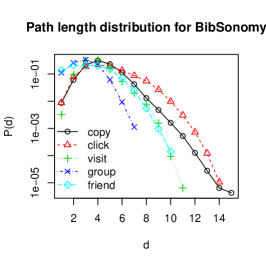
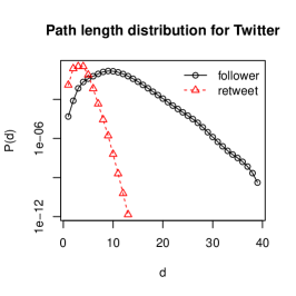
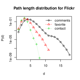
Figure 2: Distribution of the shortest path lengths in the evidence networks with logarithmically scaled counts on the $Y$-axis.

3.2 Degree Distribution

The number of adjacent nodes (degree) is one of the most important features of a node within a given network. Accordingly, the distribution of all node degrees is widely accepted as one of the key features for summarizing a given network’s connectivity kolaczyk2009statistical ; newman2003structure ; rapoport1957contribution . Figure 3 shows the cumulative degree distribution for all networks. With the exception of the Friend graph (most probably due to its limited size), all networks exhibit a long tailed degree distribution. Again, there are strong deviations among the different networks. Especially the favorite and contact networks obtained from Flickr clearly show a bias towards high degree nodes induced by the applied breadth-first crawling approach.

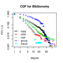
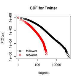
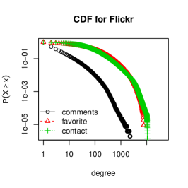
Figure 3: Logarithmically scaled cumulative degree distribution in the evidence networks.

3.3 Degree Correlation

The graph indices considered so far describe the overall structure of a network, but they do not provide insights into the individual connection structure of the network. A connection pattern which was observed in many social networks, called assortativity, homophily or mixing patterns, describes the phenomenon that similar nodes tend to connect with each other newman2003structure . This especially applies to the node degree where this property is also called degree correlation. In contrast, other types of networks, such as information networks, technical networks or biological networks, exhibit a opposite pattern, which is called disassortativity newman2003structure . Several approaches for analyzing the degree correlation in networks were proposed (see kolaczyk2009statistical for a discussion). We apply the approach proposed in pastor2001dynamical ; vazquez2002large which compactly visualizes the degree correlation by calculating the mean degree of all neighbors of a node as a function of the node degree. Formally, let $p(k^{\prime}|k)$ denote the conditional probability that a node of degree $k$ is adjacent to a node of degree $k^{\prime}$. If a network exhibits nontrivial correlations among the nodes’ degree, this conditional probability is not independent of $k$ which can be visualized by plotting the direct nearest neighbors average degree $\langle k_{nn}\rangle\mathrel{\mathop{:}}=\sum_{k^{\prime}}k^{\prime}p(k^{\prime}|k)$.

Figure 4 clearly shows a common pattern for both Twitter’s as well as Flickr’s explicit evidence networks. For lower node degrees, both networks exhibit disassortative characteristics whereas for higher degrees ($k\geq 100$) assortative mixing can be observed. Limited network sizes explain the noisy tail in all plots. In contrast, Twitter’s ReTweet graph and Flickr’s Comment graph show consistent strong assortativity. The Favorite graph shows a slight transition from disassortativity to assortativity but far less pronounced than in the explicit evidence networks. Please note that due to the sparsity of the corresponding plots induced by the limited size of all BibSonomy networks they were omitted for this analysis. In the shuffled networks, we shuffled the vertex to vertex assignments.

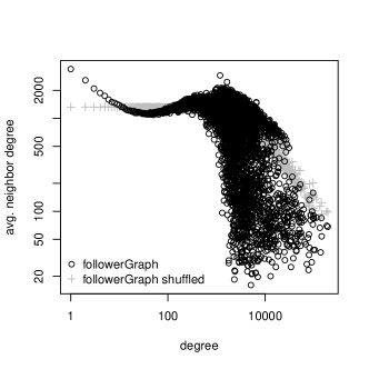
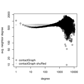
Figure 4: Nearest neighbors average degree $\langle k_{nn}\rangle$ for evidence networks in Twitter and Flickr together with $\langle k_{nn}\rangle$ averaged over five corresponding reshuffled networks.

3.4 Topological and Semantical Distance

The analysis of the last section has focused on several inherent statistical network properties of the evidence network under consideration. In this section, we will go one step further and take into account information which is not present in the networks themselves — namely background information about the semantic profile of each node. Despite the differences to a typical social network reported above, it is a natural hypothesis to assume that, e. g., two users which are close in the click network can be expected to share some common interest, which is reflected in a higher “semantic similarity” between these user nodes. In this way we establish a connection between structural properties of the respective networks and a semantic dimension of user relatedness. For measuring the “true” semantic similarity between two users we build on our prior work on semantic analysis of folksonomies markines2009evaluating , where we discovered that the similarity between tagclouds is a valid proxy for semantic relatedness. We compute this similarity in the vector space $\mathbb{R}^{T}$, in which each user is represented by the vector $v_{u}:=\bigl{(}w(u,t)\bigr{)}_{t\in T}\,$, where $w(u,t)$ is the number of times user $u$ has assigned tag $t$ to one of her resources (in case of BibSonomy and Flickr) or the number of times user $u$ has used hash tag $t$ in one of her tweets (in case of Twitter).

Each vector can be interpreted as a “semantic profile” of the respective user, represented by the distribution of her tag usage. In this vector space, we compute the cosine similarity between two vectors $\overset{\shortrightarrow}{v}_{u1}$ and $\overset{\shortrightarrow}{v}_{u2}$ according to

$$\cos\measuredangle(\overset{\shortrightarrow}{v}_{u1},\overset{\shortrightarrow}{v}_{u2})=\frac{\overset{\shortrightarrow}{v}_{u1}\cdot\overset{\shortrightarrow}{v}_{u2}}{||\overset{\shortrightarrow}{v}_{u1}||_{2}\cdot||\overset{\shortrightarrow}{v}_{u2}||_{2}}.$$

This measure is thus independent of the length of the vectors. Its value ranges from $-1$ (for vectors pointing into opposite directions) over 0 (for orthogonal vectors) to $1$ (for vectors pointing into the same direction). In our case, the similarity values lie between 0 and 1 because the vectors only contain positive numbers (refer to markines2009evaluating for details).

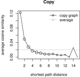
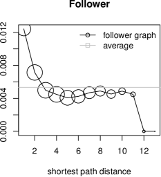
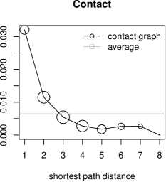
Figure 5: Average cosine similarity (y-axis) between tagclouds of users as a function of their distance in each of our networks, exemplarily for the BibSonomy Copy, the Twitter Follower and the Flickr Contact graphs. The other networks showed similar results.

As in schifanella2010folks , we plot the average semantic similarity between all pairs $(u,v)$ of users (as obtained by the cosine similarity in the tag vector space) against the shortest path between $u$ and $v$ in each of our networks – as shown in Figure 5. The size of each data point scales logarithmically with the corresponding number of shortest paths existing in the respective network. We additionally ruled out effects induced by shortest path length distribution of a network: We shuffled the feature to vertex assignment, effectively calculating the average pairwise similarity of vertex sets according to the network’s path length distribution. As expected, the shuffling process had eliminated the correlation observed before almost completely, affirming that the observed correlation of topological and semantical relatedness is not a statistical effect.

The first obvious observation is that the highest average semantic similarity is found for the smallest topological distance of one. With growing lengths of the shortest paths (x-axis), the average semantic similarity decreases quickly. In the Follower graph and all of Flickr’s networks, the similarity even drops below the global average similarity at a (topological) distance of three to four. Some networks show a peak for distant pairs (like the copy and contact graphs in Figure 5 but also the visit graph, friend graph, and comment graph). Previous work explains these peaks with the sparsity of the considered data HT2010 , specifically for the BibSonomy networks. While the larger networks do not exhibit those characteristics, e.g., the Comment graph has several thousand pairs of nodes at the corresponding distances, those peaks show only a marginal increase in the similarity and tend toward the average similarity in the whole network, as shown in the null-model plots. Furthermore, an observed bow shape in the pathlength distribution (cf. Figure 2) correlates with the corresponding similarity plot.

In summary, these results indicate a correlation of topological proximity and semantic similarity between the nodes in each of our observed networks. This confirms in a more formal way that shared interests between users are reflected in a higher degree of interaction between them — in an implicit or explicit manner.

3.5 Common Neighborhood

So far, we calculated several (descriptive) graph level statistics, and showed deviations among the global network structures. But also common patterns across the networks were revealed by analyzing the nearest neighbors average degree in the previous section. It is straightforward to consider the properties of similar nodes of different networks within a system. That is, given two evidence networks $G_{1}=(V_{1},E_{1})$ and $G_{2}=(V_{2},E_{2})$ with $V\mathrel{\mathop{:}}=V_{1}\cap V_{2}\neq\emptyset$, we compare, for each node $u\in V$ the local neighborhoods $N_{1}(u)\mathrel{\mathop{:}}=\{(u,v)\mid(u,v)\in E_{1}\}$ in $G_{1}$ and $N_{2}(u)\mathrel{\mathop{:}}=\{(u,v)\mid(u,v)\in E_{2}\}$ in $G_{2}$. We considered several similarity scores

$$J(N_{1}(u),N_{2}(u))\mathrel{\mathop{:}}={} \frac{N_{1}(u)\cap N_{2}(u)}{N_{1}(u)\cup N_{2}(u)}$$ Jaccard

$$P(N_{1}(u),N_{2}(u))\mathrel{\mathop{:}}={} \frac{N_{1}(u)\cap N_{2}(u)}{N_{1}(u)}$$ Precision

$$\cos(A_{1}[u,\,\begin{picture}(-1.0,1.0)(-1.0,-3.0)\circle*{3.0}\end{picture}\ \,],A_{2}[u,\,\begin{picture}(-1.0,1.0)(-1.0,-3.0)\circle*{3.0}\end{picture}\ \,])\mathrel{\mathop{:}}={} \frac{A_{1}[u,\,\begin{picture}(-1.0,1.0)(-1.0,-3.0)\circle*{3.0}\end{picture}\ \,]\cdot A_{2}[u,\,\begin{picture}(-1.0,1.0)(-1.0,-3.0)\circle*{3.0}\end{picture}\ \,]}{\|A_{1}\|\|A_{2}\|}$$ Cosine

where $A_{i}$ denotes the (weighted) adjacency matrix of ${G_{i}}_{|V}$, that is, $G_{i}$ reduced to the common vertex set $V$. For selected pairs of networks, Figure 6 shows the average precision score per node degree; the Jaccard index and cosine similarity yielded similar results. For contrasting the obtained result to patterns emerging from random graphs sharing the same degree distribution, each plot also shows the resulting precision score for the second network’s rewired null model, averaged over five independently generated null models.

For all considered pairs of networks, the precision profiles shows a clear deviation from the respective null models – in shape as well as in magnitude. Whereas the latter show an ascending tendency (less pronounced for the Follower-/ReTweet graph), the former show a descending (Favorites vs. Comments and Follower vs. ReTweet) or a descending to constant (Contacts versus Comments, Contacts vs. Favorites) tendency. The observed descending tendency for the Follower- and ReTweet graph means that increasing the number of social contacts does not increase the number of interactions accordingly. In contrast, a constant pattern as observed in the Contact- and Favorite graph shows, that people interact with around ten percent of their contacts, regardless of the number of their contacts.

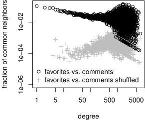
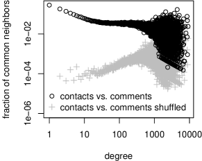
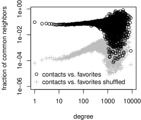
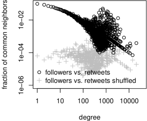
Figure 6: Precision profile for common neighborhood of different evidence networks within Twitter and Flickr.

3.6 Inter-Network Correlation Test

In the previous section, we compared pairs of networks based on local similarity per node degree. For a condensed comparison of network pairs, these similarity scores could simply be averaged. The quadradic assignment procedure (QAP) test is a standard approach for inter-network comparison common in literature; it is based on the correlation of the adjacency matrices of the considered graphs butts2008social ; BC:05 . QAP tests a given graph level statistic, for example, the graph covariance against a QAP null hypothesis.

For given graphs $G_{1}=(V_{1},E_{1})$ and $G_{2}=(V_{2},E_{2})$ with $V\mathrel{\mathop{:}}=V_{1}\cap V_{2}\neq\emptyset$ and (weighted) adjacency matrices $A_{i}$ corresponding to ${G_{i}}_{|V}$ ($G_{i}$ reduced to the common vertex set $V$, cf. Section 3.5, the graph covariance is given by

$$\mathop{cov}(G_{1},G_{2})\mathrel{\mathop{:}}=\frac{1}{n^{2}-1}\sum_{i=1}^{n}\sum_{j=1}^{n}(A_{1}[i,j]-\mu_{1})(A_{2}[i,j]-\mu_{2})\,,$$

where $\mu_{i}$ denotes $A_{i}$’s mean ($i=1,2$). Then, $\mathop{var}(G_{i})\mathrel{\mathop{:}}=\mathop{cov}(G_{i},G_{i})$ leads to the graph correlation

$$\rho(G_{1},G_{2})\mathrel{\mathop{:}}=\frac{\mathop{cov}(G_{1},G_{2})}{\sqrt{\mathop{var}(G_{1})\mathop{var}(G_{2})}}\,.$$

Table 3 shows the pairwise correlation scores for all considered networks, while Figure 7 relates this by comparison with a set of null-model experiments. All networks within BibSonomy show a quite similar level of correlation with a significant peak for the explicit Friend- and Group networks. Considering the results for the networks obtained from Flickr it is worth noting that, though low in magnitude, the Favorite graph shows a significant higher correlation with the Contact graph than the other pairs of networks do. A potential explanation considers the interaction between persons: On the one hand, people in the favorites list might be or become contacts – on the other hand the photos of contacts might be very interesting for the favorites list. But comparing the level of correlations for the different networks tells just one part of the story.

	Copy	Click	Visit	Group
Copy	$-$
Click	$0.254$	$-$
Visit	$0.214$	$0.332$	$-$
Group	$0.170$	$0.148$	$0.152$	$-$
Friend	$0.248$	$0.190$	$0.193$	$0.396$

	Comment	Favorite	Contact
Comment	$-$
Favorite	$0.006$	$-$
Contact	$0.005$	$0.074$	$-$

	ReTweet	Follower
ReTweet	$-$
Follower	$0.011$	$-$

Table 3: Pairwise graph correlation observed in BibSonomy, Flickr and Twitter.

The QAP test compares the observed graph correlation to the distribution of resulting correlation scores obtained on repeated random row/column permutations of $A_{2}$. The relative frequency of a permutation $\pi$ with a correlation $\rho^{\pi}\geq\rho_{o}$ is used for assessing the significance of an observed correlation score $\rho_{o}$. Intuitively, the test determines (asymptotically) the fraction of all graphs with the same structure as $G_{2|V}$ having at least the same level of correlation with $G_{1|V}$. Figure 7 shows the distribution of correlation scores obtained for the repeatedly permutated adjacency matrices, cf. butts2008social . For all pairs of networks, the correlation is significantly higher than one would expect by considering random graphs of the same structure (shown by the QAP test results with a zero score). These results clearly reject the null hypothesis that the degree of correlation can be explained just by $G_{2|V}$’s graph structure butts2008social . This shows the structural similarity and correlation between the different networks.

Figure 7: Distribution of the graph correlation statistic $\rho$ over 1000 permutations for selected pairs of networks.

4 Community Rating using Evidence Networks

Our comparative analysis in Section 3 suggests that the considered evidence networks exhibit deviating structural properties on a global network level but also show common local interaction patterns. In the following, we explore how evidence networks can be used to assess the quality of communities in social applications, where users collaboratively publish content. A key difficulty in assessing the quality of a given group of users is the lack of an established ground truth for measuring the level of coherency. If clusters of tags, for example, within a resource sharing system like BibSonomy are to be evaluated, external data sources such as Wikipedia or WordNet can be consulted newman2010automatic . For users there is typically no such semantic grounding. For the assessment of a community of users, gold-standard data can be applied, if available, or communities can be ranked by humans using introspection techniques for the respective user subgroups, e.g., AP:08 . Therefore, the approach presented in the following section presents a cost-effective way for assessing the ranking of community allocations using only evidence networks (secondary data) for rating the communities.

We begin with consolidating our notions and vocabulary with respect to user communities in social media. We then present our approach for rating the quality of a given community assignment and detail on the experimental setup. Finally, we present the results obtained from all considered evidence networks. The results indicate, that the inter-network correlations that we analyzed in the previous section are indeed strong enough to draw reciprocal conclusions between different evidence networks.

4.1 Community Basics

The concept of a community can be intuitively defined as a group $C$ of individuals out of a population $U$ such that members of $C$ are densely “related” to each other but sparsely “related” to individuals in $U\setminus C$. We denote a community allocation of a population $U$ as a set of communities $\mathcal{C}=\{C_{1},\ldots,C_{n}\}$ with $C_{i}\neq\emptyset$ and $\bigcup_{1\leq i\leq n}C_{i}\subseteq U$ for $1\leq i\leq n$.

In a graph $G=(V,E)$ is in this sense a vertex set $C\subseteq V$, where nodes in $C$ are densely connected but sparsely connected to nodes in $V\setminus C$. Though defined in terms of graph theory, the community concept remains vague, unless the notions of sparse and dense connectedness are specified further. Several approaches for formalizing communities in graphs exist and corresponding community structures were observed and analyzed in a variety of different networks newman2003structure ; Newman04communityStructure ; Leskovec2008 ; Leskovec2010 . For a given graph $G=(V,E)$ and a community $C\subseteq V$, we set $n\mathrel{\mathop{:}}=|V|$, $m\mathrel{\mathop{:}}=|E|$, $n_{C}\mathrel{\mathop{:}}=|C|$, $m_{C}\mathrel{\mathop{:}}=|\{(u,v)\mid u,v\in C\}|$, $\overline{m}_{C}\mathrel{\mathop{:}}=|\{(u,v)\mid u\in C,v\not\in C\}|$. For a node $u\in V$ its degree is denoted by $d(u)$. Finally, we write $G[V^{\prime}]$ for the induced subgraph of a subset $V^{\prime}\subseteq V$.

4.2 Community Quality Functions

Different quality functions $f\colon\mathcal{P}(V)\rightarrow\mathbb{R}$ for modeling the intuitive concept of a community exist (also called cluster indices). We refer to corresponding related work for more details, e. g., to Leskovec2008 and DBLP:conf/dagstuhl/Gaertler04 . This work focuses on the modularity Newman04communityStructure , the segregation index freeman1978segregation , and the conductance kannan2004clusterings .

Modularity is based on comparing the number of edges within a community with the expected number given a null-model (i. e., a randomized model). Thus, the modularity of a disjoint community clustering is defined to be the fraction of the edges that fall within the given clusters minus the expected fraction if edges were distributed at random. This can be formalized as follows: The modularity $\mathit{M}$ of a set of nodes and its assigned adjacency matrix $A\in\mathbbm{N}^{n\times n}$ is given by

$$\mathit{M}(A)=\frac{1}{2m}\sum_{i,j}\bigl{(}A_{i,j}-\frac{d(i)d(j)}{2m}\bigr{)}\delta(C_{i},C_{j})\,,$$

where $C_{i}$ is the cluster to which node $i$ belongs and $C_{j}$ is the cluster to which node $j$ belongs; $d(i)$ and $d(j)$ denote $i$ and $j$’s degrees respectively; $\delta(C_{i},C_{j})$ is the Kronecker delta symbol that equals $1$ iff $C_{i}=C_{j}$, and $0$ otherwise. For directed networks directedModularity with in- and out- degree $d(i)^{\text{in}}$ and $d(j)^{\text{out}}$ for $i$ and $j$ respectively the modularity becomes

$$\mathit{M}(A)=\frac{1}{m}\sum_{i,j}\bigl{(}A_{i,j}-\frac{d(i)^{\text{in}}d(j)^{\text{out}}}{m}\bigr{)}\delta(C_{i},C_{j})\,.$$

The modularity $\mathit{M}(A)$ obtains its maximum value $\mathit{M}(A)=1$ for a perfect partitioning, and its minimum value $\mathit{M}(A)=-1$ for the opposite.

While modularity considers the intra-cluster links compared to the corresponding null-model, the segregation index freeman1978segregation compares, for a given cluster $C$, the number of expected links accross the cluster boundary to the number of observed inter-cluster links, normalized by the expectation. By averaging the segregation over all clusters one obtains the segregation of a community allocation.

$$\mathit{S}(C)=\begin{cases}0&{}\text{if }E(\overline{m}_{C})\leq\overline{m}_{C}\\ \frac{E(\overline{m}_{C})-\overline{m}_{C}}{E(\overline{m}_{C})}&{}\text{otherwise}\end{cases}$$

The segregation index lies within the interval $[0,1]$ where higher values indicate more pronounced community structure, following the intuition that good communities are sparsely connected among each other.

Finally, the conductance captures the intuition of a “bottleneck”: If a cluster $C$ contains a non-trivial small cut (i. e., $C=C_{1}\mathaccent 0{\cdot}\cup C_{2}$ with a small value of $\overline{m}_{C}$), the cluster is probably too coarse. Otherwise, if a cluster is strongly connected to the remainder of the graph (relative to the clusters internal density), the cluster is probably too fine. The former case is assessed by a small intra-cluster conductance $\alpha(C)$ whereas the latter case corresponds to a small inter-cluster conductance $\beta(C)$. To avoid trivial cuts, both measures consider the cut size $\overline{m}_{C}$ relative to the density of the smaller subset. We define the conductance $\phi(C)$ of a community $C$ in $G=(V,E)$ and the conductance $\phi(G[V^{\prime}])$ of a subgraph $G[V^{\prime}]$ as follows:

$$\phi(C)\mathrel{\mathop{:}}= {}\begin{cases}1,&C\in\{\emptyset,V\}\\ 0,&C\not\in\{\emptyset,V\}\\ &\text{ and }\overline{m}_{C}=0\\ \frac{\overline{m}_{C}}{\min\left(\sum_{u\in C}\operatorname{d}(u),\sum_{v\in V\setminus C}\operatorname{d}(v)\right)}&\text{otherwise}\end{cases}$$

$$\phi(G[V^{\prime}])\mathrel{\mathop{:}}= {}\min_{C\subseteq V^{\prime}}\phi(C)$$

For a given clustering $C\mathrel{\mathop{:}}=\{C_{1},\ldots,C_{n}\}$, the intra-cluster conductance $\alpha(C)$ and the inter-cluster conductance $\beta(C)$ brandes2003experiments are defined accordingly.

$$\alpha(C)\mathrel{\mathop{:}}=\min_{i\in 1,\ldots,n}\phi(G[C_{i}])\quad\text{and}\quad\beta(C)\mathrel{\mathop{:}}=1-\max_{i\in 1,\ldots,n}\phi(C_{i})$$

Intra-cluster conductance was pioneered in kannan2004clusterings and found many applications in graph clustering brandes2003experiments ; spielman2004nearlylinear ; andersen2006local and community mining literature leskovec2008statistical ; Leskovec2010 . Calculating $\alpha(C)$ inherently comprises the NP-hard problem of minimizing the conductance for all cuts of a graph and thus in practice approximate algorithms must be applied. We applied the Metiskarypis1999fast graph clustering algorithm with Max-flow Quotient-cut Improvement (MQI) lang2004flowbased .

For comparing different community allocations, we consider the applied quality function as a ranking on the community allocations and apply the Kendall rank correlation coefficient kendall1938measure , which is commonly used in information retrieval for comparing different rankings. In the following we refer to it with “Kendall’s $\tau$” for short. The range is in $[-1,1]$: While $1$ indicates perfect (positive) correlation, a value of $-1$ indicates perfect negative correlation. A value of $0$ is expected for independent rankings. We discuss its application in more detail below.

4.3 Evaluation Paradigm

For the evaluation of user recommendations, Siersdorfer proposed to consult existing social structures siersdorfer2009social . We apply this paradigm to the evaluation of user communities and assess the quality of a given community allocation relative to the community structure within evidence networks. Specifically, we assume a set of users $U$ within a social application and an evidence network $G=(V,E)$ with $V\subseteq U$.

• We first mine for communities in an appropriate feature space, resulting in a community allocation

  $$\mathcal{C}=C_{1}\mathaccent 0{\cdot}\cup C_{2}\mathaccent 0{\cdot}\cup\ldots\mathaccent 0{\cdot}\cup C_{k}$$

  with $\bigcup_{C_{i}}^{i=1\ldots k}\subseteq U$.

• We then calculate some community quality function, such as modularity, within $G$ relative to $C_{1}\cap V,\ldots,C_{k}\cap V$, for an evidence network $G=(V,E)$.

Since we do not utilize a gold-standard network, the resulting score is not considered as an absolute value measuring the quality of the respective community directly. However, it induces a ranking on different community allocations on $U$ which can be used to select the top ranked allocations obtained from different clustering algorithms. In this way, it indirectly represents the quality of the respective community using the respective rankings.

Of course the question arises, whether different evidence networks and quality functions induce consistent rankings on the set of all possible community allocations. Ideally we would list all possible community allocations and calculate each quality function in every evidence network. This would result in corresponding rankings of the community allocations which then could be compared. In the best case, all rankings would coincide, whereas in the worst case all rankings would be statistically independent. Unfortunately it is not feasible to list all possible community allocations due to its combinatorial explosion. On the other hand, Monte Carlo methods would tend to compare rankings on “bad” community allocations, since the fraction of sensible allocations is very small and it is thus more likely to randomly choose an allocation which just does not make sense. We therefore chose a different practical approach. Using a broad class of different clustering methods with comprehensive parameter sets we produce as many community allocations as possible: We try to get a representative sample of all “reasonable” community allocations which is ranked accordingly for comparing the quality measures induced by the different evidence networks.

4.4 Experimentation

For mining communities, we represent every user $u$ by a vector $\overset{\shortrightarrow}{u}$ in a corresponding vector space. For the considered applications, the $i$’th component of user $\overset{\shortrightarrow}{u}$ respectively denotes, how often user $u$

• applied tag $i$ to resources (BibSonomy),

• used hash tag $i$ within tweets (Twitter) and

• applied hash tag $i$ to photographs (Flickr).

We used the freely available clustering tool Cluto. Cluto incorporates three different classes of clustering algorithms (agglomerative, partitional and graph based) which can be broadly parameterized with respect to similarity functions, normalization, number of clusters etc. We used a brute-force approach for the parametrization, resulting in 16,128 parameter combinations, out of which only a subset succeeded, due to resource limitations and due to incompatible parameter combinations. In total, we were able to collect 3,665 community allocations for BibSonomy, 993 for Twitter and 2,985 for the Flickr dataset. We calculated for each community allocation and each evidence network all of the community quality functions described in Section 4.2, namely intra-conductance, inter-conductance, modularity and segregation index. For comparison, we further constructed to each evidence network a corresponding null model by randomly rewiring pairs of edges maslov2002specificity . In these null model networks, clustering and community structure is destroyed while the degree distribution of the networks is fixed. Rankings induced by these networks are thus independent of the respective community structure. We averaged corresponding quality functions over five independently constructed null model graphs.

For summarizing the consistency between a pair of induced rankings, we calculate Kendall’s $\tau$ as described above. The drawback of such a global measure is that all positions are considered equally important. Yet, in our case we are mainly interested in the top ranked positions, since they are expected to be the “most reasonable” cluster assignments. For assessing the consistency between two rankings in more detail, we calculate the size of the overlap of the two rankings, considering only the top $k$ positions FKS:03 ; for example, we consider how many community allocations are placed in both rankings among the top $10$ positions. The absolute figures alone are hard to interpret, as we expect a certain overlap merely by statistical effects (consider, e. g., the case were $n=k$).

We therefore compare our results with the expected overlap assuming two randomly ordered rankings. Let $\pi_{1}$ and $\pi_{2}$ be two random permutations on {1, …, n}, and let $m$ denote the number of common community allocations among the top $k$ positions, i. e., $m\mathrel{\mathop{:}}=|\{C_{\pi_{1}(1)},\ldots,C_{\pi_{1}(k)}\}\cap\{C_{\pi_{2}(1)},\ldots,C_{\pi_{2}(k)}\}|$. This corresponds to a random sampling process without replacement. There are $\binom{k}{m}$ possible combinations of $m$ common elements among the top $k$ positions. The remaining $k-m$ top elements can be chosen out of $n-k$ community allocations which are not contained in $\{C_{\pi_{1}(1)},\ldots,C_{\pi_{1}(k)}\}$, that is $\binom{k}{m}\cdot\binom{n-k}{k-m}$ options exist. Normalizing by the number of possible rankings of length $k$ we obtain

$$P(m)=\frac{\binom{k}{m}\cdot\binom{n-k}{k-m}}{\binom{n}{k}}$$

which is a special case ($n_{1}=n_{2}=k$) of the hypergeometric distribution $h(m;n,n_{1},n_{2})$ with mean $n_{1}\frac{n_{2}}{n}$. The expected size of the overlap is therefore given by $\frac{k^{2}}{n}$.

For all considered systems and evidence networks, nearly all community allocations obtained a inter-conductance score of (almost) 0. This is due to the sparsity of evidence networks: As communities are mined independently of the evidence networks, most clusters contain more than one component when mapped into the evidence network which leads to a corresponding minimal conductance value of 0. We therefore exclude inter-conductance from presentation below.

4.4.1 BibSonomy

Using the BibSonomy tagging data we clustered the set of users in the feature space where each user is represented by a vector corresponding to the user’s tag cloud. This resulted in $3,665$ community allocations. We calculated for each community allocation intra-conductance, modularity and segregation index in every evidence network (Friend graph, Group graph, Copy graph, Click graph, Visit graph). We thus obtained 15 different rankings on all community allocations.

For intra-conductance, all networks but the Group graph induced trivial rankings as nearly all community assignments obtained a zero score. Therefore, we exclude the intra-conductance rankings in BibSonomy from further considerations. Figure 8 shows the distribution of obtained quality function scores, exemplarily using the Click graph. Modularity and segregation index both induce a large number of high quality communities in all networks. In the distributions in the Click graph example, the overall majority focuses on high quality communities indicating the existing community structure.

Figure 8: Distribution of the quality functions exemplarily shown for the BibSonomy Click graph.

Table 4 shows Kendall’s $\tau$ calculated on all pairs of all rankings induced by the different quality functions. The lower left triangle shows the correlation coefficient (Kendall’s Tau) for pairs were one network’s community structure was destroyed by randomly rewiring links (averaged over five repetitions). Considering modularity, the resulting correlation coefficients indicate significantly correlated rankings among all pairs of networks which is absent when one network is shuffled. This indicates that different networks assess community structure consistently (to a certain extent) in terms of modularity and that the ranking is in fact dependent on the community structure of the network. Correlation coefficients for rankings induced by segregation on the other hand do not indicate similar correlations and the obtained correlation coefficients for rewired networks do not support the required dependence on the network’s community structure.

Modularity:

	Click	Copy	Friend	Group	Visit
Click	-0.430	0.806	0.820	0.798	0.822
Copy	-0.453	-0.194	0.769	0.747	0.775
Friend	-0.429	-0.199	0.250	0.784	0.767
Group	-0.423	-0.206	0.242	0.450	0.741
Visit	-0.370	-0.175	0.222	0.413	-0.407

Segregation:

	Click	Copy	Friend	Group	Visit
Click	-0.013	0.011	0.036	0.069	0.016
Copy	0.020	-0.013	-0.080	0.048	-0.036
Friend	-0.019	-0.014	-0.075	0.030	0.067
Group	-0.074	-0.022	0.026	0.028	-0.011
Visit	-0.020	0.027	-0.095	0.010	0.021

Table 4: Kendall’s $\tau$ correlation coefficient for modularity and segregation based rankings relative to evidence networks in BibSonomy. For $i\leq j$ the lower triangle shaded in gray shows the correlation for rankings induced by network $j$ and network $i$’s null models.

Finally, Figure 9 details on the dependence of observed correlation on the relative position within the ranking, exemplarily for selected pairs of networks. Firstly, we note that for modularity induced rankings the overlap between the top $k$ positions is consistently very high and better than the expected overlap (cf. Section 4.4 above), as shown by the the bold lines above the main diagonal close to the “max overlap” line. If the induced rankings are meaningful with respect to their inherent community structure, the rankings should depend on the community structure and not on statistical properties of the network which merely result from the network’s degree distribution. For that, we calculated for each network the induced rankings on corresponding randomly rewired networks (in which the community structure is destroyed) maslov2002specificity . The respective overlap curve is given in Fig. 9 as the bold dashed line (“null model”). Furthermore, the correlation coefficients consistently indicate significant correlations with increasing magnitude for larger $k$.

Secondly, the overlap with rankings induced by rewired networks show varying behavior for the different networks. Comparing the rankings induced by the Click graph and the Visit graph, the null-model overlap consistently lies below the expected overlap for independent rankings whereas it coincides with the expected null-model overlap only in the beginning for both other pairs of networks.

Alltogether, the correlation coefficients indicate independence in rankings for all null-model rankings. These findings indicate a consistent relative ranking behavior in the BibSonomy networks, which is also confirmed by the null-model experiments.

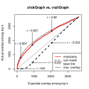
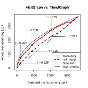
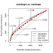
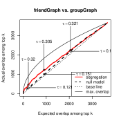
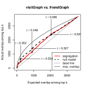
Figure 9: Comparison between two rankings by considering the size of the intersection between the corresponding top $k$ entry set. The plot shows, how much the actual overlap deviates from the expected overlap if the rankings were randomly ordered.

4.4.2 Twitter

Applying the same set of clustering algorithms as for BibSonomy resulted in $993$ clustering models for Twitter; as described above, the smaller number of community allocations – compared to the BibSonomy dataset – is explained by the fact that during application of the algorithms and parametrizations of the Cluto toolkit many algorithms did not terminate correctly due to resource limitations. Figure 10 shows the distribution of all applied quality functions in all considered networks. Again, modularity and segregation index both lead to a broad range of quality function scores. It is worth noting that the modularity distribution does not exhibit a sharply pronounced peak at level 0 as in the case of BibSonomy.

Figure 10: Distribution of the quality functions for the follower graph in Twitter.

Table 5 shows as in the case for BibSonomy Kendall’s $\tau$ rank correlation coefficient for all pairs of networks as well as corresponding null models. For rankings induced by intra-conductance and segregation index, Kendall’s $\tau$ suggests independence, whereas for rankings induced by modularity, significantly higher correlation is observed than in corresponding null model experiments. These observations are in line with those for BibSonomy.

Modularity:

	ReTweet	Follower
ReTweet	0.057	0.658
Follower	0.443	0.097

Intra-Conductance:

	ReTweet	Follower
ReTweet	-0.012	-0.027
Follower	0.024	-0.018

Segregation:

	ReTweet	Follower
ReTweet	-0.005	0.049
Follower	0.000	0.004

Table 5: Kendall’s $\tau$ correlation coefficient for modularity and segregation based rankings relative to evidence networks in Twitter. For $i\leq j$ the lower triangle shaded in gray shows the correlation for rankings induced by network $j$ and network $i$’s null models.

Figure 11 visualizes these results. Only the modularity induced rankings show a clear distinction between the rankings induced by the original graphs and the corresponding null models, indicating that the obtained rankings are indeed dependent on the network’s community structure.

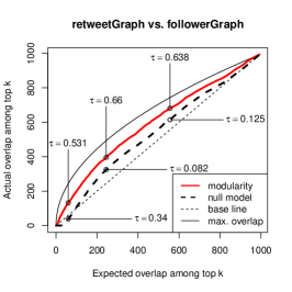
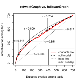
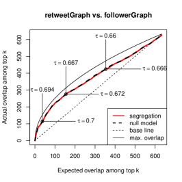
Figure 11: Comparison between rankings by considering the size of the intersection between the corresponding top $k$ entry set in Twitter: Modularity (left), intra-conductance (middle) and segregation index (right).

Fig. 11 plots the actual overlap between the top $k$ positions of the rankings induced by Twitter’s Follower graph and the ReTweet graph versus the size of the expected overlap if the rankings were independent (cf. Section 4.4 above). As for the BibSonomy networks, we also calculated for each network the induced rankings on corresponding randomly rewired networks (in which the community structure is destroyed) maslov2002specificity . The respective overlap curve is given in Fig. 11 as the bold dashed line (“null model”). Exemplary Fig. 11 additionally shows Kendall’s $\tau$ for the two sequences of common community allocations between the top $234$ elements (first quarter in the plots) of the rankings induced by twitter’s follower and retweet network (with a $p$ value $p<10^{-6}$) showing a very strong correspondence between the two rankings. Again, these results confirm the consistent relative ranking of the community allocations as we have observed for the BibSonomy networks above.

4.4.3 Flickr

For the Flickr dataset, the applied clustering algorithms resulted in $2,985$ community allocations. Figure 12 shows the distribution of quality function scores for all considered networks. Again, modularity and segregation index show a broad range of quality scores whereas (due to sparsity) intra-conductance only assessed low quality communities. Most notably, the distribution of modularity show a clear separation between lower and higher quality ranked community allocations in the Comment graph whereas the Favorites graph and the Contacts graph does not induce such a pronounced bimodal distribution. Rankings induced by the segregation index show a bimodal distribution for all considered networks.

Figure 12: Distribution of the quality functions in all networks in Flickr.

Table 6 shows the averages of Kendall’s $\tau$ over every network and all pairs of networks together with corresponding null model graphs for modularity and segregation index. Again only for modularity, the correlation coefficient suggests strong correlations among rankings obtained in different networks which is missing when community structure is destroyed in corresponding null models.

Modularity:

	Comment	Favorite	Contact
Comment	-0.029	0.789	0.811
Favorite	-0.151	-0.220	0.944
Contact	-0.152	-0.007	-0.016

Segregation:

	Comment	Favorite	Contact
Comment	0.027	0.034	0.034
Favorite	0.014	-0.004	0.028
Contact	0.016	-0.023	-0.013

Table 6: Kendall’s $\tau$ correlation coefficient for modularity and segregation based rankings relative to evidence networks in Flickr. The upper triangle shows the correlations between the different networks. For $i<j$ the shaded lower triangle shows the correlation for rankings induced by network $j$ and network $i$’s null models, i. e., comparing the shuffled networks.

These results are again visualized in Figure 13. Again, these results confirm the findings obtained by the BibSonomy and Twitter analysis.

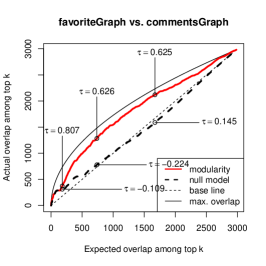
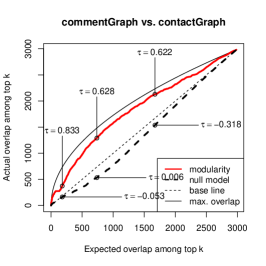
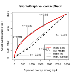
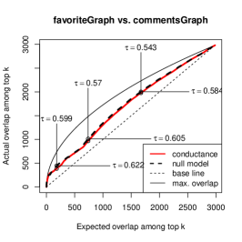
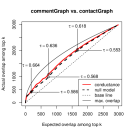
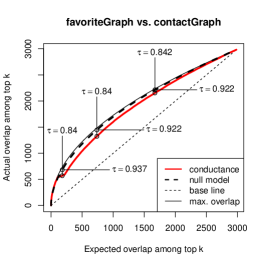
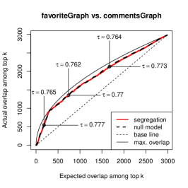
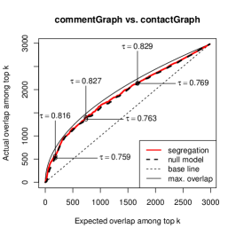
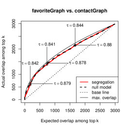
Figure 13: Comparison between two rankings by considering the size of the intersection between the corresponding top $k$ entry set in Flickr: Modularity (top), intra-conductance (middle) and segregation index (bottom).

4.5 Discussion

The applied paradigm of evaluating against existing social structures has the significant advantage, that the assessment of community allocations are relative to explicitly established social links (e. g., friendship links in BibSonomy); their intention is multifaceted as it is the case for the underlying social constellation. On the other hand, evidence networks as introduced in this work could directly be used for finding and evaluating communities. The main drawback would be, that evidence networks typically only cover a certain amount of the users (in case of the friendship network in BibSonomy only $12$%). Additionally, most community detection algorithms try to optimize a given objective function which assesses the quality of the community allocations and there is a risk that the method thus optimizes towards community allocations biased by the applied objective function (e. g., communities which contain half of the users in case of modularity Leskovec2010 ). Thus, the proposed method separates the objective function used for optimizing the community allocation from the quality function used for assessing it.

The experimental results presented in the previous section indicate that implicit evidence networks used for assessing the quality of a community structure are surprisingly consistent with the expected behavior as formalized by the existing explicit social structures, in particular concerning the Friend graph.

In our experiments, we observed a high correlation between the quality measures calculated on the implicit and explicit networks supporting this hypothesis. Furthermore, in our experiments, modularity provided always the best results in contrast to the conductance or the segregation index measures. Therefore, based on our findings, we would always recommend modularity as a quality measure for the ranking based assessment method.

5 Related Work

In the following, we discuss related approaches concerning the analysis of network structure, communities, and implicit link structures in different systems and networks.

Analyzing Web 2.0 data by applying complex network theory goes back to the analysis of (samples from) the web graph broder2000graph . Mislove et al. mislove2007measurement applied methods from social network analysis as well as complex network theory and analyzed large scale crawls from prominent social networking sites. Some properties common to all considered social networks are worked out and contrasted to properties of the web graph. Newman analyzed many real life networks, summing up characteristics of social networks newman2003social . The analysis of online social media, the interrelations of the involved actors, and the involved geospatial extents have attracted a lot of attention during the last decades, especially for the microblogging system Twitter. A thorough analysis of fundamental network properties and interaction patterns in Twitter can be found in kwak2010twitter .

Interdependencies of social links and geospatial proximity are investigated in scellato2011sociospatial ; mcgee2011geographic ; kaltenbrunner2012eyes , especially concerning the correlation of the probability of friendship links and the geographic distance of the corresponding users. Silva et al. SWZ:10 mine structural correlation patterns in network partitions, i. e., correlations between vertex attributes and dense components in undirected graphs. While their approach results in individual patterns, our analysis captures both patterns and the networks/graphs as a whole and provides comprehensive analysis on their combined structure.

Schifanella et al. schifanella2010folks investigated the relationship of topological closeness (in terms of the length of shortest paths) with respect to the semantic similarity between the users, while similarity measures in the context of semantic analysis of folksonomies are evaluated in markines2009evaluating . We adapt these approaches for our setting.

Leroy et al. LCB:10 discusses a feature-based approach using implicit information for inferring interaction networks in the context of link prediction. Eagle et al. EPL:09 describe an approach for reconstructing friendship relations from secondary (mobile phone) data. They show, that friendship links can be inferred with a high probability but do not present a comprehensive analysis of different evidence networks and their impact on the predictability. Barrat et al. barrat2010lss discuss the relation between online and offline networks. Similarly, Chin et al. DBLP:conf/socialcom/ChinWXZWZ11 consider ephemeral networks of encounters for inferring contact networks, however, no relations to other evidence networks are discussed.

Another aspect of our work is the analysis of implicit link structures which can be obtained in a running Web 2.0 system and how they relate to other existing link structures, i. e., evidence networks. Butts and Carley BC:05 describe simple algorithms for structural comparisons between different kinds of structured objects. Furthermore, Baeza-Yates et al. baeza2007extracting propose to present query-logs as an implicit folksonomy where queries can be seen as tags associated to documents clicked by people making those queries. The authors extracted semantic relations between queries from a query-click bipartite graph; nodes are queries and an edge between nodes exists when at least one equal URL has been clicked after submitting the query. Krause et al. krause2008logsonomy analyzed term-co-occurrence-networks in the logfiles of internet search systems.

Fortunato and Castellano Fortunato2007 discuss various aspects connected to the concept of community structure in graphs. Basic definitions as well as existing and new methods for community detection are presented. In Lancichinetti2009 , Lancichinetti and Fortunato present a thorough comparison of many different state of the art community detection algorithms for graphs. The performance of algorithms are compared relative to a class of adequately generated artificial benchmark graphs. Karamolegkos et al. Karamolegkos20091498 introduced metrics for assessing user relatedness and community structure by means of the normalized size of user profile overlaps. They evaluate their metrics in a live setting, focussing on the optimization of the given metrics. Using a metric which is purely based on the structure of graphs, Newman presents algorithms for finding communities and assessing community structure in graphs Newman:2004 . A thorough empirical analysis of the impact of different community mining algorithms and their corresponding objective function on the resulting community structures is presented in Leskovec2010 , which is based on the size resolved analysis of community structure in graphs as presented in Leskovec2008 . In the context of this paper, we do not focus on the identification of communities. In contrast, we propose a method for the relative ranking and assessment of communities based on our findings on structural inter-network correlations.

6 Conclusions

The contribution of this paper can be summarized as follows: We introduce evidence networks as a new tool for structural assessment in social applications and show that there are structural inter-network correlations that allow reciprocal conclusions between the different networks. Furthermore, our conducted experiments suggest that the different networks are not contradictory but complementary. The evidence networks are thoroughly analyzed with respect to the contained community structure (cf. Section 3). It is shown that there is a strong common community structure across different networks.

Furthermore, using standard community evaluation measures, we showed that there is a strong common community structure across different networks; the induced rankings are reciprocally consistent. Therefore, we proposed a method for the relative ranking of communities for their assessment. In general, the task of automatically finding and recognizing meaningful community allocations on a set $U$ of users is still an open problem. Due to the multifaceted characteristics of user relatedness it is impossible to define “the best” community allocation. Therefore, the assessment of the quality of a given community is thus always application dependent and relative to certain aspects of user relatedness, e. g., race of individuals in newman2003structure , shared topical interests in social bookmarking systems, or social traces manifested in the evidence networks.

Specifically, the presented analysis is thus not only relevant for the evaluation of community mining techniques, but also for implementing new community detection or user recommendation algorithms, among others. The context of the presented analysis is given by social media applications such as social networking, social bookmarking, and social resource sharing systems, considering the Twitter microblogging service, our own system BibSonomy Bibs:VLDB10 , and the Flickr resource sharing system as examples.

For future work, we aim to investigate, how the single evidence networks can be suitably combined into a weighted network. For this, we need to further analyze the individual structure of the networks, and the possible interactions. As another direction of research, we plan to incorporate evidence networks in the community detection process (e. g., in terms of constraints).

References

- (1) Andersen, R., Chung, F., Lang, K.: Local graph partitioning using pagerank vectors. In: Proceedings of the 47th Annual IEEE Symposium on Foundations of Computer Science, pp. 475–486. IEEE Computer Society, Washington, DC, USA (2006). DOI 10.1109/FOCS.2006.44
- (2) Atzmueller, M., Puppe, F.: A Case-Based Approach for Characterization and Analysis of Subgroup Patterns. Journal of Applied Intelligence 28(3), 210–221 (2008)
- (3) Baeza-Yates, R., Tiberi, A.: Extracting Semantic Relations from Query Logs. In: Proc. 13th ACM SIGKDD Conference, p. 85. ACM (2007)
- (4) Barrat, A., Cattuto, C., Szomszor, M., den Broeck, W.V., Alani, H.: Social Dynamics in Conferences: Analysis of Data from the Live Social Semantics Application. In: Proc. 9th International Semantic Web Conference (ISWC 2010) (2010)
- (5) Becchetti, L., Castillo, C., Donato, D., Fazzone, A., Rome, I.: A comparison of sampling techniques for web graph characterization. In: Proceedings of the Workshop on Link Analysis (LinkKDD’06), Philadelphia, PA (2006)
- (6) Benz, D., Hotho, A., Jäschke, R., Krause, B., Mitzlaff, F., Schmitz, C., Stumme, G.: The Social Bookmark and Publication Management System BibSonomy – A Platform for Evaluating and Demonstrating Web 2.0 Research. J. VLDB 19, 849–875 (2010)
- (7) Brandes, U., Gaertler, M., Wagner, D.: Experiments on graph clustering algorithms. In: Proc. ESA 2003, 11th Annual European Symposium, Budapest, Hungary, LNCS, vol. 2832, pp. 568–579 (2003)
- (8) Broder, A., Kumar, R., Maghoul, F., Raghavan, P., Rajagopalan, S., Stata, R., Tomkins, A., Wiener, J.: Graph Structure in the Web. Computer Networks 33(1-6), 309–320 (2000)
- (9) Butts, C.: Social network analysis: A methodological introduction. Asian Journal of Social Psychology 11(1), 13–41 (2008)
- (10) Butts, C., Carley, K.: Some Simple Algorithms for Structural Comparison. Computational & Mathematical Organization Theory 11, 291–305 (2005)
- (11) Butts, C.T., Carley, K.M.: Some simple algorithms for structural comparison. Comput. Math. Organ. Theory 11, 291–305 (2005). DOI 10.1007/s10588-005-5586-6
- (12) Chin, A., Wang, H., Xu, B., Zhang, K., Wang, H., Zhu, L.: Connecting People in the Workplace through Ephemeral Social Networks. In: Proc. PASSAT/SocialCom 2011: 2011 IEEE Third International Conference on Privacy, Security, Risk and Trust (PASSAT), and 2011 IEEE Third International Conference on Social Computing (SocialCom), pp. 527–530. IEEE (2011)
- (13) Diestel, R.: Graph Theory. Springer, Berlin (2006)
- (14) Eagle, N., Pentland, A., Lazer, D.: Inferring Friendship Network Structure by using Mobile Phone Data. Proceedings of the National Academy of Sciences 106(36), 15,274–15,278 (2009). DOI 10.1073/pnas.0900282106
- (15) Fagin, R., Kumar, R., Sivakumar, D.: Comparing Top k Lists. In: Proc. 14th Annual ACM-SIAM Symposium on Discrete Algorithms, SODA ’03, pp. 28–36. Society for Industrial and Applied Mathematics, Philadelphia, PA, USA (2003)
- (16) Fortunato, S., Castellano, C.: Community Structure in Graphs (2007). Arxiv:0712.2716 Chapter of Springer’s Encyclopedia of Complexity and System Science
- (17) Freeman, L.: Segregation In Social Networks. Sociological Methods & Research 6(4), 411 (1978)
- (18) Gaertler, M.: Clustering. In: U. Brandes, T. Erlebach (eds.) Network Analysis, LNCS, vol. 3418, pp. 178–215. Springer (2004)
- (19) Gjoka, M., Kurant, M., Butts, C.T., Markopoulou, A.: Practical Recommendations on Crawling Online Social Networks . IEEE J. Sel. Areas Commun. on Measurement of Internet Topologies (2011)
- (20) Kaltenbrunner, A., Scellato, S., Volkovich, Y., Laniado, D., Currie, D., Jutemar, E.J., Mascolo, C.: Far From the Eyes, Close on the Web: Impact of Geographic Distance on Online Social Interactions. In: Proc. ACM SIGCOMM Workshop on Online Social Networks (WOSN 2012). Helsinki, Finland (2012)
- (21) Kannan, R., Vempala, S., Vetta, A.: On clusterings: Good, bad and spectral. J. ACM 51(3), 497–515 (2004). DOI 10.1145/990308.990313
- (22) Karamolegkos, P.N., Patrikakis, C.Z., Doulamis, N.D., Vlacheas, P.T., Nikolakopoulos, I.G.: An Evaluation Study of Clustering Algorithms in the Scope of User Communities Assessment. Computers & Mathematics with Applications 58(8), 1498–1519 (2009)
- (23) Karypis, G., Kumar, V.: A fast and high quality multilevel scheme for partitioning irregular graphs. SIAM Journal on Scientific Computing 20(1), 359 (1999)
- (24) Kendall, M.G.: A New Measure of Rank Correlation. Biometrika 30(1/2), 81–93 (1938)
- (25) Kolaczyk, E.D.: Statistical Analysis of Network Data: Methods and Models, 1st edn. Springer, Heidelberg, Germany (2009)
- (26) Krackhardt, D.: Computational Organization Theory, chap. Graph Theoretical Dimensions of Informal Organizations, p. 89–111. Lawrence Erlbaum, NJ (1994)
- (27) Krause, B., Jäschke, R., Hotho, A., Stumme, G.: Logsonomy - Social Information Retrieval with Logdata. In: Proc. 19th Conf. on Hypertext and Hypermedia, pp. 157–166. ACM (2008)
- (28) Kwak, H., Lee, C., Park, H., Moon, S.: What is twitter, a social network or a news media? In: Proceedings of the 19th international conference on World wide web, pp. 591–600. ACM (2010)
- (29) Lancichinetti, A., Fortunato, S.: Community Detection Algorithms: A Comparative Analysis (2009). Arxiv:0908.1062
- (30) Lang, K., Rao, S.: A flow-based method for improving the expansion or conductance of graph cuts. Integer Programming and Combinatorial Optimization pp. 383–400 (2004)
- (31) Leicht, E.A., Newman, M.E.J.: Community Structure in Directed Networks. Phys. Rev. Lett. 100(11) (2008)
- (32) Leroy, V., Cambazoglu, B.B., Bonchi, F.: Cold Start Link Prediction. In: Proc. 16th ACM SIGKDD International Conference on Knowledge Discovery and Data Mining, KDD ’10, pp. 393–402. ACM, New York, NY, USA (2010)
- (33) Leskovec, J., Lang, K.J., Dasgupta, A., Mahoney, M.W.: Community Structure in Large Networks: Natural Cluster Sizes and the Absence of Large Well-Defined Clusters (2008). Arxiv:0810.1355
- (34) Leskovec, J., Lang, K.J., Dasgupta, A., Mahoney, M.W.: Statistical properties of community structure in large social and information networks. In: J. Huai, R. Chen, H.W. Hon, Y. Liu, W.Y. Ma, A. Tomkins, X. Zhang (eds.) WWW, pp. 695–704. ACM (2008). DOI 10.1145/1367497.1367591
- (35) Leskovec, J., Lang, K.J., Mahoney, M.W.: Empirical Comparison of Algorithms for Network Community Detection (2010). Arxiv:1004.3539
- (36) Markines, B., Cattuto, C., Menczer, F., Benz, D., Hotho, A., Stumme, G.: Evaluating similarity measures for emergent semantics of social tagging. In: 18th Int’l WWW Conference, pp. 641–641 (2009)
- (37) Maslov, S., Sneppen, K.: Specificity and stability in topology of protein networks. Science 296(5569), 910 (2002)
- (38) McGee, J., Caverlee, J.A., Cheng, Z.: A Geographic Study of Tie Strength in Social Media. In: Proc. 20th ACM International Conference on Information and Knowledge Management, CIKM ’11, pp. 2333–2336. ACM, New York, NY, USA (2011)
- (39) Mislove, A., Marcon, M., Gummadi, K., Druschel, P., Bhattacharjee, B.: Measurement and Analysis of Online Social Networks. In: 7th ACM SIGCOMM Conf. on Internet Measurement, p. 42. ACM (2007)
- (40) Mitzlaff, F., Benz, D., Stumme, G., Hotho, A.: Visit Me, Click Me, Be My Friend: An Analysis of Evidence Networks of User Relationships in Bibsonomy. In: Proceedings of the 21st ACM Conference on Hypertext and Hypermedia (2010)
- (41) Newman, D., Lau, J.H., Grieser, K., Baldwin, T.: Automatic evaluation of topic coherence. In: Human Language Technologies: The 2010 Annual Conference of the North American Chapter of the Association for Computational Linguistics, pp. 100–108. Association for Computational Linguistics, Los Angeles, California (2010)
- (42) Newman, M., Park, J.: Why Social Networks are different from Other Types of Networks. Physical Review E 68(3), 36,122 (2003)
- (43) Newman, M.E., Girvan, M.: Finding and Evaluating Community Structure in Networks. Phys Rev E Stat Nonlin Soft Matter Phys 69(2), 1–15 (2004)
- (44) Newman, M.E.J.: The structure and function of complex networks. SIAM Review 45(2), 167–256 (2003)
- (45) Newman, M.E.J.: Detecting Community Structure in Networks. Europ Physical J 38 (2004)
- (46) Pastor-Satorras, R., Vázquez, A., Vespignani, A.: Dynamical and correlation properties of the Internet. Physical Review Letters 87(25) (2001)
- (47) Rapoport, A.: Contribution to the theory of random and biased nets. Bulletin of Mathematical Biology 19, 257–277 (1957). DOI 10.1007/BF02478417
- (48) Scellato, S., Noulas, A., Lambiotte, R., Mascolo, C.: Socio-spatial properties of online location-based social networks. Proceedings of ICWSM 11, 329–336 (2011)
- (49) Schifanella, R., Barrat, A., Cattuto, C., Markines, B., Menczer, F.: Folks in Folksonomies: Social Link Prediction from Shared Metadata. In: Proc. 3rd ACM Int’l Conf. on Web search and data mining, pp. 271–280. ACM, New York, NY, USA (2010)
- (50) Siersdorfer, S., Sizov, S.: Social Recommender Systems for Web 2.0 Folksonomies. In: HT09: Proc. 20th ACM Conf. on Hypertext and Hypermedia, pp. 261–270. ACM, New York, NY, USA (2009)
- (51) Silva, A., Meira, W., Zaki, M.J.: Structural Correlation Pattern Mining for Large Graphs. In: Proceedings of the Eighth Workshop on Mining and Learning with Graphs, MLG ’10, pp. 119–126. ACM, New York, NY, USA (2010)
- (52) Spielman, D., Teng, S.: Nearly-linear time algorithms for graph partitioning, graph sparsification, and solving linear systems. In: Proceedings of the thirty-sixth annual ACM symposium on Theory of computing, pp. 81–90. ACM (2004)
- (53) Vázquez, A., Pastor-Satorras, R., Vespignani, A.: Large-scale Topological and Dynamical Properties of the Internet. Physical Review E 65(6) (2002)
- (54) Yang, J., Leskovec, J.: Patterns of temporal variation in online media. In: Proceedings of the fourth ACM international conference on Web search and data mining, pp. 177–186. ACM (2011)