Fundamental solutions of MHD Stokes flow

Abstract

A simple analytical solution is obtained for the MHD stokeslet in a homogeneous magnetic field. This solution represents the flow past a small particle and can also be interpreted as the flow sufficiently far away from a body of finite size. Fundamental solutions are found in terms of velocity, pressure and scalar potential distributions for the flows due to either a concentrated force or a current source. The former consists of two basic solutions for the force parallel and transverse to the magnetic field, respectively. All fundamental solutions have the characteristic length scale of the Hartmann boundary layer and two parabolic wakes developing along the magnetic field.

Applied Mathematics Research Centre, Coventry University, Coventry, CV1 5FB, UK

1 Introduction

The non-linear inertial effects in the flows of conducting liquids may become negligible not only at low velocities but also in strong enough magnetic fields [1]. Numerical computation of such flows is still complicated by the fine and intricate meshing required to resolve the thin boundary and free shear layers that develop in complex geometries. Owing to the linearity such flows can also be computed using the boundary integral equation (BIE) techniques, which requires only the surface but no volume meshing. This is approach is well developed for Stokes flows in classical hydrodynamics [2] but not so in magnetohydrodynamics [3, 4]. The problem is the so-called fundamental solution, which is essential for the BIE formulation and describes the flow due to a concentrated point-force. Such a fundamental solution, which plays the same role as the Coulomb’s law in the electrostatics and is known as a stokeslet in the hydrodynamics [5], is still missing in the MHD. The aim of the present study is to fill in this gap.

2 Formulation of problem

Consider an unbounded flow of a viscous electrically conducting liquid in a homogeneous magnetic field $\mbox{\boldmath${B}$}.$ The flow is due a body which may be either dragged through the liquid by a constant force ${F}$ or discharging a direct current $I,$ which then interacts with the externally applied magnetic field. The interaction of the current with its own magnetic field is supposed to be negligible. Sufficiently far away from the body, the flow is expected to be independent of the body size and shape, and determined only by the total force and the current. Thus, ${F}$ and $I$ are assumed to be concentrated at the body location $\mbox{\boldmath${x}$}_{0},$ and the Dirac delta function $\delta(\mbox{\boldmath${x}$}-\mbox{\boldmath${x}$}_{0})$ is used for their density distributions. The origin of the coordinate system is set at the body location so that $\mbox{\boldmath${x}$}_{0}=\mbox{\boldmath${0}$},$ and a simplified notation $\delta(\mbox{\boldmath${x}$})\equiv\delta$ introduced. Neglecting the non-linear inertial forces, which supposes either a creeping flow or a sufficiently strong magnetic field, the flow is governed by the linearised Navier–Stokes equation with the electromagnetic body term

$$\eta\mbox{\boldmath${\nabla}$}^{2}\mbox{\boldmath${v}$}-\mbox{\boldmath${\nabla}$}p+\mbox{\boldmath${j}$}\times\mbox{\boldmath${B}$}=-\mbox{\boldmath${F}$}\delta,$$ (1)

where the velocity ${v}$ is subject to the incompressibility constraint $\mbox{\boldmath${\nabla}$}\cdot\mbox{\boldmath${v}$}=0.$ The current obeys both the Ohm’s law for a moving medium $\mbox{\boldmath${j}$}=\sigma(-\mbox{\boldmath${\nabla}$}\phi+\mbox{\boldmath${v}$}\times\mbox{\boldmath${B}$})$ and the charge conservation $\mbox{\boldmath${\nabla}$}\cdot\mbox{\boldmath${j}$}=I\delta.$ The latter results in Poisson’s equation for the electric potential $\phi:$

$$\mbox{\boldmath${\nabla}$}^{2}\phi-\mbox{\boldmath${B}$}\cdot\mbox{\boldmath${\nabla}$}\times\mbox{\boldmath${v}$}=-I\delta.$$ (2)

The resulting flow represents a superposition of mechanically and electrically driven flows, which owing to the linearity of the problem are mutually independent and, thus, are considered separately. Subsequently, these two flow components are denoted by the indices $v$ and $\phi.$ Henceforth, we change to the dimensionless variables by using the Hartmann layer thickness $d=B^{-1}\sqrt{\eta/\sigma}$ as the length scale and $v_{0}=d^{2}F/\eta$ and $v_{0}=IB/\eta$ as characteristic velocities for the flows driven mechanically and electrically. Other quantities are scaled, respectively, by $p_{0}=v_{0}\eta/d,$ $j_{0}=v_{0}\eta/(d^{2}B),$ and $\phi_{0}=v_{0}dB,$ where $B=|\mbox{\boldmath${B}$}|$ and $F=|\mbox{\boldmath${F}$}|.$ The directions of the magnetic field and force are specified by the unit vectors $\mbox{\boldmath${\beta}$}=\mbox{\boldmath${B}$}/B$ and $\mbox{\boldmath${f}$}=\mbox{\boldmath${F}$}/F.$ Governing equations (1) and (2) can be written in dimensionless form as

$$\mbox{\boldmath${\nabla}$}^{2}\mbox{\boldmath${v}$}-\mbox{\boldmath${\nabla}$}p+\mbox{\boldmath${\beta}$}\times(\mbox{\boldmath${\nabla}$}\phi+\mbox{\boldmath${\beta}$}\times\mbox{\boldmath${v}$})=-\left[\begin{array}[]{l}\delta\\ 0\end{array}\right]\mbox{\boldmath${f}$};\qquad\mbox{\boldmath${\nabla}$}^{2}\phi-\mbox{\boldmath${\beta}$}\cdot\mbox{\boldmath${\nabla}$}\times\mbox{\boldmath${v}$}=-\left[\begin{array}[]{l}0\\ \delta\end{array}\right],$$ (3)

where the upper and lower cases on the r.h.s correspond to mechanically and electrically driven flows. Applying the operators

$$\mbox{\boldmath${\mathcal{L}}$}_{v}^{v}=\mbox{\boldmath${\nabla}$}\times\mbox{\boldmath${\nabla}$}\times,\quad\mathcal{L}_{p}^{v}=\left[\mbox{\boldmath${\nabla}$}^{2}\mbox{\boldmath${\nabla}$}-\mbox{\boldmath${\beta}$}\cdot\mbox{\boldmath${\nabla}$}\mbox{\boldmath${\beta}$}\right]\cdot,\quad\mathcal{L}_{\phi}^{v}=\mbox{\boldmath${\nabla}$}\cdot\mbox{\boldmath${\beta}$}\times$$ (4)

to the first equation (3) and taking into account the second equation (3), results in separate equations for each variable

$$\left[\mbox{\boldmath${\nabla}$}^{4}-(\mbox{\boldmath${\beta}$}\cdot\mbox{\boldmath${\nabla}$})^{2}\right]\{\mbox{\boldmath${v}$},p,\phi\}^{\{v,\phi\}}=\mbox{\boldmath${\mathcal{L}}$}^{\{v,\phi\}}\delta,$$ (5)

where the operator indices are expanded as follows

$$\mbox{\boldmath${\mathcal{L}}$}^{\{v,\phi\}}\equiv\left[\begin{array}[]{l}\mbox{\boldmath${\mathcal{L}}$}^{v}\mbox{\boldmath${f}$}\\ \mbox{\boldmath${\mathcal{L}}$}^{\phi}\mathcal{I}\end{array}\right]\equiv\left[\begin{array}[]{l}\{\mbox{\boldmath${\mathcal{L}}$}_{v}^{v},\mathcal{L}_{p}^{v},\mathcal{L}_{\varphi}^{v}\}\mbox{\boldmath${f}$}\\ \{\mbox{\boldmath${\mathcal{L}}$}_{v}^{\phi},\mathcal{L}_{p}^{\phi},\mathcal{L}_{\phi}^{\phi}\}\mathcal{I}\end{array}\right],$$ (6)

and the operators with the superscript $\varphi$ referring to the electrically driven flow are

$$\mbox{\boldmath${\mathcal{L}}$}_{v}^{\phi}=\mbox{\boldmath${\beta}$}\times\mbox{\boldmath${\nabla}$},\quad\mathcal{L}_{p}^{\phi}=0,\quad\mathcal{L}_{\phi}^{\phi}=\mathcal{I}-\mbox{\boldmath${\nabla}$}^{2}.$$ (7)

Since both the l.h.s and r.h.s operators in (5) are linear constant-coefficient operators and, thus, interchangeable with each other, the solution of (5) can written as

$$\{\mbox{\boldmath${v}$},p,\phi\}^{\{v,\phi\}}=\mbox{\boldmath${\mathcal{L}}$}^{\{v,\phi\}}G,$$ (8)

where $G$ is the fundamental solution satisfying

$$\left[\mbox{\boldmath${\nabla}$}^{4}-(\mbox{\boldmath${\beta}$}\cdot\mbox{\boldmath${\nabla}$})^{2}\right]G=\delta.$$ (9)

3 Fundamental solution

For the sake of simplicity we further assume the $z$-axis to be directed along the magnetic field so that $\mbox{\boldmath${\beta}$}=\mbox{\boldmath${e}$}_{z}$ and $(\mbox{\boldmath${\beta}$}\cdot\mbox{\boldmath${\nabla}$})^{2}\equiv\partial_{z}^{2}.$ Firstly, it is important to note that (9) can be factorised in two ways as

$$\left[\mbox{\boldmath${\nabla}$}^{2}\pm\partial_{z}\right]G\, = -G_{\pm},$$ (10)

$$\left[\mbox{\boldmath${\nabla}$}^{2}\mp\partial_{z}\right]G_{\pm}\!\!\! = -\delta.$$ (11)

Secondly, the substitution $G_{\pm}=\mathrm{e}^{(\pm z-R)/2}G_{0},$ where $R=|\mbox{\boldmath${x}$}|$ is the spherical radius, reduces (11) to $\mbox{\boldmath${\nabla}$}^{2}G_{0}=-\delta,$ whose fundamental solution is the well-known Coulomb potential

$$G_{0}(\mbox{\boldmath${x}$})=1/4\pi R.$$ (12)

Adding and subtracting (10) with different signs, results in

$$\mbox{\boldmath${\nabla}$}^{2}G =-\frac{1}{2}(G_{+}+G_{-})= -\cosh(z/2)\mathrm{e}^{-R/2}G_{0},$$ (13)

$$\partial_{z}G =-\frac{1}{2}(G_{+}-G_{-})= -\sinh(z/2)\mathrm{e}^{-R/2}G_{0}.$$ (14)

Equation (14) can be integrated as

$$G(\mbox{\boldmath${x}$})=\int\partial_{z}G\,\mathrm{d}z=-\frac{1}{8\pi}\left[E_{1}((R+z)/2)+E_{1}((R-z)/2)\right]+q(r),$$ (15)

where $E_{1}(x)=\int_{x}^{\infty}t^{-1}\mathrm{e}^{-t}\,\mathrm{d}t$ is the exponential integral and $q$ is a ‘constant’ of integration. The latter is a function of the cylindrical radius $r=\sqrt{R^{2}-z^{2}},$ and satisfies the homogeneous counterpart of (9). It is determined as $q(r)=-\ln r/4\pi$ by removing the logarithmic singularity $E_{1}(x)\sim-\ln x,$ which appears in (15) at the symmetry axis because $x=R-|z|\rightarrow 0$ when $r\rightarrow 0.$ The Laplacian and the $z$-component of the gradient of $G$, which are required in (8), are given by (13) and (14), respectively. The missing $r$-component of the gradient can be obtained by differentiating (15) and expressed in terms of the previous two quantities and (12) as

$$\partial_{r}G=-(R\mbox{\boldmath${\nabla}$}^{2}G+z\partial_{z}G)/r-1/4\pi r.$$ (16)

For the following, it is important to note that the first term on the r.h.s depends only on the cylindrical radius $r$ and decreases inversely with $r$, whereas the second term similar to (13) and (14) depends also on the axial coordinate $z$ and falls off exponentially at large $r.$

3.1 Mechanically driven flow

Axial force

Owing to the linearity of the problem, the mechanically induced flow can be represented as a superposition of particular solutions due to the force components parallel and perpendicular to the magnetic field. In the following, these solutions are referred to as axial and transverse ones. The former is obtained by taking $\mbox{\boldmath${f}$}=\mbox{\boldmath${e}$}_{z}$ in (5), which results in $\mbox{\boldmath${\mathcal{L}}$}_{\{v,p,\phi\}}^{v}\mbox{\boldmath${e}$}_{z}G=\{\mbox{\boldmath${V}$},P,\Phi\}_{z}^{v},$ where

$$\mbox{\boldmath${V}$}_{z}^{v}=\mbox{\boldmath${\nabla}$}\times(\mbox{\boldmath${e}$}_{\varphi}\Psi_{\varphi z}^{v});\qquad P_{z}^{v}=-(3zR^{-1}\mbox{\boldmath${\nabla}$}^{2}G+\partial_{z}G)/2;\qquad\Phi_{z}^{v}=0.$$ (17)

Axisymmetric poloidal velocity (17) is defined by the azimuthal component of the stream function $\Psi_{\varphi z}^{v}=-\partial_{r}G.$ The instantaneous streamlines of this flow, which are represented by the isolines of $r\Psi_{\varphi z}^{v},$ are shown in Fig. 1(a) together with the pressure distribution $P_{z}^{v}.$ Note that no electric potential is induced because the e.m.f generated by such an axisymmetric poloidal flow is purely azimuthal and, thus, solenoidal. As seen, the flow is confined in the regions where the argument of the exponential functions in (13,14) is not too small, i.e. $R\pm z\lesssim 1.$ For the large axial distances $|z|\gtrsim 1$, these regions correspond to two parabolic wakes $r^{2}\lesssim|z|,$ which extend along the magnetic field in both directions from the origin. In the mid-plane (|$z|\lesssim 1),$ the solution drops off exponentially over the cylindrical radius $r\sim 1,$ which is the dimensionless thickness of the Hartmann layer. Along the axis $(r=0)$, (17) yields

$$P_{z}^{v}=-(3\mbox{\boldmath${\nabla}$}^{2}G+\partial_{z}G)/2=(2+\mathrm{e}^{-|z|})/8\pi z,\quad V_{zz}^{v}=r^{-1}\partial_{r}(r\partial_{r}G)=(1+z-\mathrm{e}^{-|z|})/8\pi z|z|,$$ (18)

according to which both the pressure and the axial velocity drop off as $\sim z^{-1}.$ The incompressibility and the confinement of the flow within the parabolic wakes of the radius $r\sim|z|^{1/2}$ results in the radial velocity component decreasing as $V_{rz}^{v}\sim z^{-3/2}.$

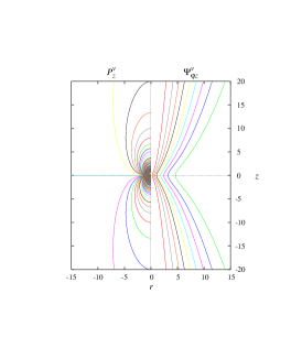
Figure 1: Axial solutions for the pressure $P_{z}^{v}$ and the stream function $\Psi_{z}^{v}$ shown at $r<0$ and $r>0,$ respectively (a). Pressure distribution $P_{x}^{v}$ and the transverse stream function $\Psi_{yx}^{v}$ in the $xz$-plane shown at $x<0$ and $x>0,$ respectively, (b), and axial stream function $\Psi_{yx}^{v}$ in the $xy$-plane $(y<0)$ and the electric potential $\Phi_{x}^{v}=-\Psi_{zx}^{v}$ $(y>0)$ in the $yz$-plane (c).

Transverse force

In this case solution is obtained by taking $\mbox{\boldmath${f}$}=\mbox{\boldmath${e}$}_{x},$ which results in $\mbox{\boldmath${\mathcal{L}}$}_{\{v,p,\phi\}}^{v}\mbox{\boldmath${e}$}_{x}G=\{\mbox{\boldmath${V}$},P,\Phi\}_{x}^{v},$ where

$$\mbox{\boldmath${V}$}_{x}^{v}=\mbox{\boldmath${\nabla}$}\times(\mbox{\boldmath${e}$}_{y}\Psi_{yx}^{v}+\mbox{\boldmath${e}$}_{z}\Psi_{zx}^{v}),\quad P_{x}^{v}=\mbox{\boldmath${e}$}_{x}\cdot\mbox{\boldmath${\nabla}$}\mbox{\boldmath${\nabla}$}^{2}G=-\frac{3x}{2R}\mbox{\boldmath${\nabla}$}^{2}G,\quad\Phi_{x}^{v}=-\Psi_{zx}^{v}=\frac{y}{r}\partial_{r}G.$$ (19)

In this case, the flow, which is three-dimensional and has all three velocity components, is described by two components of the stream function. Isolines of the transverse component $\Psi_{yx}^{v}=\partial_{z}G$ represent the streamlines of the solenoidal part of the flow in the planes parallel to both the magnetic field and the force, describes the circulation in the $xz$-plane with the streamlines shown in Fig. 1(b) at $x>0.$ The $z$-component of the stream function, which coincides with the induced electric potential in (19), describes circulation in the plane transverse to the magnetic field, i.e. the $xy$-plane in the case under consideration. Streamlines in this plane are shown in Fig. 1(c) $(y<0)$ together with the potential distribution in the $yz$-plane $(y>0).$ The pressure in (19), whose distribution in the $xz$-plane is plotted in Fig. 1(b) at $x<0,$ shows the characteristic two-wake structure. Comparing this pressure with (20) it is not hard to see that in the wakes with $r\sim z^{1/2}$ the pressure drops off as $\sim z^{-3/2}.$ The transverse velocity component along the axis is

$$V_{xx}^{v}=\partial_{x}\Psi_{zx}^{v}-\partial_{z}\Psi_{yx}^{v}=-\mbox{\boldmath${\nabla}$}^{2}G=(1+\mathrm{e}^{-|z|})/8\pi|z|,$$ (20)

which is in the same direction as the force. However, as seen in Fig. (1)(b) $(x>0)$, the circulation in the plane of the magnetic field and force is directed oppositely to the latter with the associated transverse velocity varying as

$$-\partial_{z}\Psi_{yx}^{v}=-\partial_{z}^{2}G=-(1-(1+|z|)\mathrm{e}^{-|z|})/8\pi z^{2},$$

which at large distances drops off as $\sim z^{-2}.$ This decrease is faster than $\sim z^{-1}$ for the total transverse velocity (20), which includes also the circulation transversely to the magnetic field in the plane $xy$-plane. Thus, the latter obviously dominates at large axial distances.

The solutions for $\Phi_{x}^{v}$ and $\Psi_{zx}^{v},$ which according to (19) differ from each other only by the sign, are substantially different from the solutions considered so far. The difference is due to the first term in (16), which as noted above falls off at large cylindrical radii algebraically as $\sim r^{-1}.$ In particular, for the mid-plane $z=0,$ the expressions in (19) reduce to

$$\Phi_{x}^{v}=-\Psi_{zx}^{v}=\sin\varphi(\mathrm{e}^{-r/2}-1)/4\pi r,$$

where $\sin\varphi=y/r.$ Thus, in contrast the other variables considered above, $\Phi_{x}^{v}$ and $\Psi_{zx}^{v}$ fall off outside the wakes as $\sim r^{-1}$ rather than exponentially, and thus, as seen in Fig. 1(c), they are not confined in the wakes.

References

• [1] Branover, G. G. and Tsinober, A. B.: Magnetohydrodynamics of incompressible media, Moscow: Nauka 1970 (in Russian).
• [2] Pozrikidis, C.: Boundary integral and singularity methods for linearized viscous flows, Cambridge: Cambridge University Press 1992.
• [3] Tsinober, A. B.: Axisymmetric magnetohydrodynamic Stokes flow in a half-space, Magnetohydrodynamics 4 (1973) 450–461.
• [4] Tsinober, A. B.: Green’s function for axisymmetric MHD Stokes flow in a half-space, Magnetohydrodynamics 4 (1973) 559–561.
• [5] Hasimoto, H. and Sano, O.: Stokeslets and eddies in creeping flow, Ann. Rev. Fluid Mech. 12 (1980) 335–63.