Revisiting Optimal Power Control: Its Dual Effect on SNR and Contention

Abstract

In this paper we study a transmission power-tune/control problem in the context of 802.11 Wireless Local Area Networks (WLANs) with multiple (and possibly densely deployed) access points (APs). Previous studies on power control tend to focus on one aspect of the control, either its effect on transmission capacity (PHY layer effect) assuming simultaneous transmissions, or its effect on contention order (MAC layer effect) by maximizing spatial reuse. We observe that power control has a dual effect: it affects both spatial reuse and capacity of active transmission; moreover, maximizing the two separately is not always aligned in maximizing system throughput and can even point in opposite directions. In this paper we introduce an optimization formulation that takes into account this dual effect, by measuring the impact of transmit power on system performance from both PHY and MAC layers. We show that such an optimization problem is intractable and develop an analytical framework to construct simple yet efficient solutions. Through numerical results, we observe clear benefits of this dual-effect model compared to solutions obtained that try to maximize spatial reuse and transmission capacity separately. This problem does not invoke cross-layer design, as the only degree of freedom in design resides with transmission power. It however highlights the complexity in tuning certain design parameters, as the change may manifest itself differently at different layers which may be at odds.

We further form a game theoretical framework and investigate above power-tune problem in a strategic network. We show that with decentralized and strategic users, the Nash Equilibrium (N.E.) of the corresponding game is in-efficient and thereafter we propose a punishment based mechanism to enforce users to adopt the social optimal strategy profile under both perfect and imperfect sensing environments.

I Introduction

Power-tune has emerged as an important issue in an IEEE 802.11 WLAN network of multiple interacting users (Access Points, or APs). Earlier classical results with focus on power-tune may be classified into the following two independent approaches.

The first relies on a PHY-layer framework in interference-bounded networks, i.e., the optimal power-tune problem is defined with respect to the Signal-Noise-Ratio (SNR) of each AP or the entire network. Within this framework, each AP’s transmission power has two contradicting roles: The first is that a higher transmission power will improve the noise resistance capability for its own communication and thus potentially the network capacity. The other role is the unavoidable interaction with other APs. A higher transmission power will contribute higher noise/interference to other APs using the same channel (we assume Orthogonal Frequency Division Multiplexing, OFDM, at PHY layer and thus we will not consider intra-channel interference). Many results have been established in this framework with different techniques focusing on either centralized or distributed solutions.

The second class of results stems from MAC layer techniques by trying to reduce the level of contention within a network, or improving spatial reuse order, as more generally referred to. Specifically, when users fall into each other’s audible range, transmission back-off under CSMA/CA is triggered to resolve contention and enable sharing. Therefore, decreasing users’ transmission range helps improve spatial reuse of a given channel. It follows that they are often modeled as congestion games or other similar graph problems (more in Section VII).

Even though conceptually both frameworks aim at optimizing system performance, e.g., overall throughput, the technical objectives and thus the net impact under the two are clearly not always aligned, and in fact can be quite different and even point in opposite directions. To illustrate, consider maximizing users’ achievable throughput or capacity without considering the induced spatial contention relationship; the resulting power-tune can create areas of very high contention order. Thus, even though a user’s (or the network’s) transmission capacity/rate maybe maximized on a per transmission basis, significant amount of air time may be spent in the back-off process instead of data transmission, leading to wasted spectrum resources. The opposite may also be true. If we simply control the contention topology of the network, the transmission power settings may be such that users do not have sufficient noise resistance capability and thus fall short of the theoretically achievable capacity. In this case, even though we may have successfully reduced the contention and saved a lot of air time, the quality of active transmissions (or on a per-transmission basis) may be low.

In short, reducing transmission power has a dual effect on the MAC and PHY layers: it can help increase spatial reuse order under CSMA/CA, but can at the same time decrease noise resistance capacity and therefore the transmission capacity. A desirable solution should thus take both effects into consideration in determining the optimal power control. This is strictly speaking not a cross-layer problem, as the only degree of freedom in design resides with transmission power, i.e., there is no joint design or feedback between different layers. This problem simply highlights the complexity in tuning certain design parameters, as the change may manifest itself differently at different layers which could be self-defeating as illustrated above.

In this study we approach this problem by introducing a performance measure (or utility function) based on the power-tune impact on both PHY and MAC layers simultaneously. An interesting technical aspect of this formulation is the combination of both continuous (SNR and PHY) and discrete (MAC or graph-based) elements in a single optimization problem. Not surprisingly, this leads to an intractable optimization problem, whose properties and structures we then investigate to help construct good and efficient solution techniques. Extensive simulation is conducted to verify the effectiveness and performance of our solution approach. An equally important aspect of our study, besides solving the above optimization problem, is to obtain insight into how the resulting power-tune differs from the two approaches outlined earlier, each focusing on the effect on a single layer, respectively.

Our formulation and solution are given within a centralized framework. A natural next step is to examine distributed implementations of the solution, and similar optimization problems when users are strategic. These remain interesting directions of future research, but are out of the scope of the present paper.

The remainder of the paper is organized as follows. Section II gives the system model and problem formulation, while Section III characterizes the optimal solution. Section VI provides extensive numerical results to evaluate our approach. Section VII presents a literature review most relevant to the present study and Section VIII concludes the paper.

II System model

II-A Preliminaries

Consider a WLAN network with $N$ APs denoted by the set $\Omega=\{1,2,...,N\}$. Each AP is associated with a number of stations with whom it communicates. Denote an AP’s transmission power space (i.e., the set of power levels it may employ) by $\mathcal{Q}_{i},i\in\Omega$. Different from many prior works, here we do not assume any finiteness of $\mathcal{Q}_{i}$; instead, we will show that the finiteness of the optimal power profile follows naturally from our formulation. We will assume $\mathcal{Q}_{i},i\in\Omega$ are all closed and use $\overline{\mathcal{P}}_{i}$ and $\underline{\mathcal{P}}_{i}$ to denote the maximum and minimum value in $\mathcal{Q}_{i}$, respectively. The transmission power profile of all users is denoted by $\mathcal{P}=[\mathcal{P}_{1},\mathcal{P}_{2},...,\mathcal{P}_{N}]$.

Each AP also has a certain attempt rate for channel access under IEEE 802.11, and these are denoted by the vector $\mathbf{p}:=[p_{1},p_{2},...,p_{N}]$, also referred to as the attempt rate profile. Channel gain (or path loss) from user $i$ to $j$ is denoted by $h_{ij}$. We will assume $h_{ij},i,j\in\Omega$ stay unchanged during a single transmission; alternatively, we may view $h_{ij}$ as the expectation of channel dynamics. $\mathcal{N}_{0}$ denotes the average noise level, and $\mathcal{P}^{i}_{cs}$ denotes the carrier sensing (CS) threshold of the $i-$th AP.

For the rest of the paper we will use the terms AP and user interchangeably.

II-B Contention domain

Due to the fact that many hardware/circuits put a requirement on CS signal’s strength, some CS signals cannot be correctly decoded and the corresponding back-off actions will not be triggered; only those with strength higher than the CS threshold can be correctly identified. We thus define two notions of a contention domain for user/AP $i$. The first one $\Delta^{r}_{i}$, the receive contention domain, is the set of users/APs whose CS signals can be correctly decoded by user $i$; while the other $\Delta^{t}_{i}$, the transmit contention domain, is the set of users who can decode user $i$’s CS signals correctly. Mathematically we have

$$\Delta^{r}_{i}=\{j:\mathcal{P}_{j}\cdot h_{ji}\geq\mathcal{P}^{i}_{cs},j\in\Omega\backslash\{i\}\}$$ (1)

$$\Delta^{t}_{i}=\{j:\mathcal{P}_{i}\cdot h_{ij}\geq\mathcal{P}^{j}_{cs},j\in\Omega\backslash\{i\}\}$$ (2)

By definition, contention domain is closely related to spatial reuse. With a larger contention domain, the degree of spatial reuse is potentially smaller around that user. Define $n_{i}(\mathbf{\mathcal{P}})$ to be the number of competing users of user $i$ under power profile $\mathbf{\mathcal{P}}$; i.e., $n_{i}(\mathbf{\mathcal{P}}):=|\Delta^{r}_{i}|$. This will also be referred to as the contention order for user $i$.

II-C Neighborhood reaching threshold

Consider AP $i$ and the maximum (resp. minimum) transmission power it can use without reaching (resp. so that it can still reach) another AP $k$, expressed as follows (assumed to exist):

$${\mathcal{P}}^{-}_{ik}: =\max\{\mathcal{P}_{i}:\mathcal{P}_{i}\cdot h_{ik}<\mathcal{P}^{k}_{cs},\mathcal{P}_{i}\in\mathcal{Q}_{i}\}$$ (3)

$${\mathcal{P}}^{+}_{ik}: =\min\{\mathcal{P}_{i}:\mathcal{P}_{i}\cdot h_{ik}\geq\mathcal{P}^{k}_{cs},\mathcal{P}_{i}\in\mathcal{Q}_{i}\}~{}.$$ (4)

To make it complete for $k=i$ we have

$${\mathcal{P}}^{-}_{ii}: =\underline{\mathcal{P}}_{i},{\mathcal{P}}^{+}_{ii}:=\overline{\mathcal{P}}_{i}$$ (5)

Denote the set of these neighbors reaching thresholds for AP $i$ as

$$\tilde{\mathcal{Q}}_{i}=\cup_{k\in\Omega}\{{\mathcal{P}}^{-}_{ik},{\mathcal{P}}^{+}_{ik}\}.$$ (6)

Denote the neighbor reaching profile space for the whole network as

$$\tilde{\mathcal{Q}}:=\tilde{\mathcal{Q}}_{1}\times\tilde{\mathcal{Q}}_{2}\times...\times\tilde{\mathcal{Q}}_{N}~{}.$$ (7)

Since we are considering a finite size network (i.e., the number of APs, $N$, is a finite positive integer), this profile space is finite, i.e., $|\tilde{\mathcal{Q}}_{i}|<\infty,\forall i\in\Omega$, and consequently $|\tilde{\mathcal{Q}}|<\infty$.

II-D A performance measure/utility function

From AP $i$’s point of view, its transmission power setting has the following implications:

• Higher transmission power will increase AP $i$’s received SNR ($\text{SNR}_{i}$) by its associated stations.

• Higher transmission power will cause higher interference to APs outside $\Delta^{r}_{i}\cup\Delta^{t}_{i}$.

• Higher transmission power will add $i$ to some other AP $j$’s contention domain.

As a result, AP $i$’s perceived performance, or utility $\mathcal{U}_{i}$, as a function of the transmission power profile ${\mathcal{P}}$ and attempt rate profile $\mathbf{p}$ across all APs, may be captured by the following expression:

$$\mathcal{U}_{i}(\mathbf{\mathcal{P}},\mathbf{p})=\mathcal{S}_{i}(\mathbf{\mathcal{P}},\mathbf{p})\cdot\mathcal{C}_{i}(\mathbf{\mathcal{P}},\mathbf{p}),~{}~{}~{}i\in\Omega,$$ (8)

where $\mathcal{S}_{i}$ is the “sharing” function representing AP $i$’s share of channel access under CSMA/CA-type of collision avoidance mechanism, and $\mathcal{C}_{i}$ is the “capacity” function representing the rate/quality of active transmissions under $\mathbf{\mathcal{P}}$ and $\mathbf{p}$.

Under 802.11, we can approximate $\mathcal{S}_{i}$ using the probability of successful channel reservation given by $\prod_{j\in\Delta^{r}_{i}}(1-p_{j})p_{i}$, where the dependence on the transmission power profile ${\mathcal{P}}$ is implicit through the contention domain $\Delta^{r}_{i}=\Delta^{r}_{i}({\mathcal{P}})$. Assuming a fair WLAN network with $0<p_{1}=p_{2}=...=p_{N}=p_{c}<1$, we then have the following form of the sharing function:

$$\mathcal{S}_{i}(\mathbf{\mathcal{P},\mathbf{p}})=\prod_{j\in\Delta^{r}_{i}}(1-p_{j})p_{i}=(1-p_{c})^{n_{i}(\mathcal{P})}p_{c},$$ (9)

which approximates the air time share of AP $i$ within its contention domain.

$\mathcal{C}_{i}$ is intended to capture the rate or capacity of active transmission attained by AP $i$. To make this concrete, we will focus on the downlink capacity from the AP to its associated stations. As the stations’ locations can change dynamically and are often unknown, we will not explicitly model this level of detail and simply assume that the stations are sufficiently close to their associated AP. Consequently, their capacity may be approximated using the transmit power by the AP (rather than the received power at a station) and the interference at the AP (rather than at a station), in the standard Shannon formula: (similar formulation can also be found in [8]):

$$\mathcal{C}_{i}(\mathbf{\mathcal{P}},\mathbf{p})=\log(1+\frac{\mathcal{P}_{i}}{\mathcal{N}_{0}+\sum_{j\in\bar{\Delta}^{r}_{i}\cap\bar{\Delta}^{t}_{i}}\mathcal{S}_{j}(\mathbf{\mathcal{P},\mathbf{p}})\cdot\mathcal{P}_{j}\cdot h_{ji}})~{},$$ (10)

where $\bar{\Delta}^{r}_{i}$ ($\bar{\Delta}^{t}_{i}$) denotes the complement of AP $i$’s contention domains, i.e., $\bar{\Delta}^{r}_{i}=\Omega_{-i}\backslash\Delta^{r}_{i}$, reflecting the fact that the interference comes primarily from APs outside the contention domain as a result of the back-off mechanism of IEEE 802.11 collision avoidance.

III The optimal power-tune problem and its characterization

In this section, we formally define our optimization problem and do so in comparison with its single-layer counterparts, i.e., that aim at only the PHY or MAC layer effect, respectively. We then characterize its features using a two-user example.

III-A Considering only PHY layer effects

When we limit our attention to PHY layer effects of power control, typically no contention is considered and parallel transmissions are implicitly assumed. Therefore each single user’s transmissions will contribute to other users noise/interference. Problems along this line have been well investigated in the literature, see e.g., [8, 2]. Specifically these assumptions result in the following optimization problem

$$\begin{array}[]{ccll}\textbf{(PPHY)}&\max&\sum_{i\in\Omega}\log(1+\frac{\mathcal{P}_{i}}{\mathcal{N}_{0}+\sum_{j\neq i}\mathcal{P}_{j}\cdot h_{ji}})\\ &\text{s.t.}&\mathcal{P}_{j}\in\mathcal{Q}_{i},\forall i\in\Omega.\end{array}$$

This rate maximization problem is in general hard to solve. Previous work has focused on different approximation techniques, see e.g., [8]. In order to obtain comparable results in order to compare this with our optimization formulation, in our numerical experiments (Section VI) we shall use the following simple approximation

$$\log(1+\frac{\mathcal{P}_{i}}{\mathcal{N}_{0}+\sum_{j\neq i}\mathcal{P}_{j}\cdot h_{ji}})\approx\log(\frac{\mathcal{P}_{i}}{\mathcal{N}_{0}})-\frac{\sum_{j\neq i}\mathcal{P}_{j}\cdot h_{ji}}{\mathcal{N}_{0}}$$ (11)

Since both terms $\log(\frac{\mathcal{P}_{i}}{\mathcal{N}_{0}})$ and $-\frac{\sum_{j\neq i}\mathcal{P}_{j}\cdot h_{ji}}{\mathcal{N}_{0}}$ are concave, we now have an approximate/relaxed optimization problem which is convex:

$$\begin{array}[]{ccll}\textbf{(R-PPHY)}&\max&\sum_{i\in\Omega}\{\log(\frac{\mathcal{P}_{i}}{\mathcal{N}_{0}})-\frac{\sum_{j\neq i}\mathcal{P}_{j}\cdot h_{ji}}{\mathcal{N}_{0}}\}\\ &\text{s.t.}&\mathcal{P}_{j}\in\mathcal{Q}_{i},\forall i\in\Omega.\end{array}$$

This problem can be efficiently solved using classical convex optimization techniques (assuming all $\mathcal{Q}_{i}$ are convex or piece-wise convex). These are used in our numerical results provided later, and the algorithmic details are omitted for brevity.

III-B Considering only MAC layer effects

We next limit our attention to MAC layer effects of power control, in which case the objective is typically to minimize the sum of contention orders over all users, given as follows:

$$\min\sum_{i\in\Omega}n_{i}(\mathcal{P})~{},$$ (12)

see, e.g., a similar objective used in [10]. However, without any constraint on $\mathcal{P}$, the above minimization could lead to somewhat pathologic solutions, i.e., with very low power, we can obtain $\sum_{i\in\Omega}n_{i}(\mathcal{P})\approx 0$ thereby achieving the minimum value. However, with very low transmission powers and relatively constant background noise, each AP’s SNR is significantly impacted leading to poor transmission performance. Consequently, in order to make this model comparable with others considered in our numerical experiments, we will instead consider a similar optimization problem with an SNR constraint. Specifically, we will try to minimize the total contention order within the network, subject to a minimum requirement on each AP’s SNR, as shown below:

$$\begin{array}[]{ccll}\textbf{(PMAC)}&\min&\sum_{i\in\Omega}n_{i}(\mathcal{P})\\ &\text{s.t.}&\frac{\mathcal{P}_{i}}{\mathcal{N}_{0}+\sum_{j\in\bar{\Delta}^{r}_{i}\cap\bar{\Delta}^{t}_{i}}S_{j}(\mathbf{\mathcal{P},\mathbf{p}})\cdot\mathcal{P}_{j}\cdot h_{ji}}\geq\text{SNR}_{0},\\ &&\forall i\in\Omega.\end{array}$$

Here we use $\text{SNR}_{0}$ to denote some baseline SNR that needs to be met at each AP’s transmission.

The above problem has a mixture of a combinatorial term and continuous term in the following sense: while the SNR is continuous w.r.t. setting transmission power $\mathcal{P}_{i}$, the contention domains $\Delta_{i}$s are discrete. Thus the problem is hard to solve in general. We thus consider a relaxation of the above problem. Since we have

$$\mathcal{P}_{j}\cdot h_{ji}<\mathcal{P}^{i}_{cs},\forall j\in\bar{\Delta}^{r}_{i}\cap\bar{\Delta}^{t}_{i}~{},$$ (13)

the inequality below holds immediately

$$\sum_{j\in\bar{\Delta}^{r}_{i}\cap\bar{\Delta}^{t}_{i}}S_{j}(\mathbf{\mathcal{P},\mathbf{p}})\cdot\mathcal{P}_{j}\cdot h_{ji}<\sum_{j\in\bar{\Delta}^{r}_{i}\cap\bar{\Delta}^{t}_{i}}S_{j}(\mathbf{\mathcal{P},\mathbf{p}})\cdot\mathcal{P}^{i}_{cs}$$ (14)

Moreover, we have

$$\frac{\mathcal{P}_{i}}{\mathcal{N}_{0}+\sum_{j\in\bar{\Delta}^{r}_{i}\cap\bar{\Delta}^{t}_{i}}\mathcal{P}_{j}\cdot h_{ji}}>\frac{\mathcal{P}_{i}}{\mathcal{N}_{0}+\sum_{j\in\bar{\Delta}^{r}_{i}\cap\bar{\Delta}^{t}_{i}}S_{j}(\mathbf{\mathcal{P},\mathbf{p}})\cdot\mathcal{P}^{i}_{cs}}.$$ (15)

Thus, we have the following relaxed problem that are solvable:

$$\begin{array}[]{ccll}\textbf{(R-PMAC)}&\min&\sum_{i\in\Omega}n_{i}(\mathcal{P})\\ &\text{s.t.}&\frac{\mathcal{P}_{i}}{\mathcal{N}_{0}+\sum_{j\in\bar{\Delta}^{r}_{i}\cap\bar{\Delta}^{t}_{i}}S_{j}(\mathbf{\mathcal{P},\mathbf{p}})\cdot\mathcal{P}^{i}_{cs}}\geq\text{SNR}_{0},\forall i\in\Omega.\end{array}$$

Theorem III.1

In solving R-PMAC there is no loss of optimality to limit our attention to the space $\tilde{\mathcal{Q}}$, i.e., if an optimal solution exists, we can always find an optimal solution within the space $\tilde{\mathcal{Q}}$.

Proof 1

Suppose there is an optimal power profile with some element, say $\mathcal{P}^{*}_{j}\notin\tilde{\mathcal{Q}}_{j}$. Then consider relaxing/increasing $\mathcal{P}^{*}_{j}$ to the nearest ${\mathcal{P}}^{-}_{jk},\forall k\in\Omega$. Note that such a change would not modify the contention topology and thus all $n_{i}$ values remain the same, without violating the corresponding SNR constraint. Thus we have found an optimal solution within $\tilde{\mathcal{Q}}$.

Remark III.2

This theorem allows us to focus on a finite set of solutions instead of all possible solutions.

III-C Considering dual effects

We now formalize the optimal power-tune problem outlined earlier that takes into account both the PHY and MAC layer effects. Specifically, we will seek centralized solutions to the following social welfare maximization problem:

$$\begin{array}[]{ccll}\textbf{(P)}&\max&\mathcal{U}=\sum_{i\in\Omega}\mathcal{U}_{i}(\mathbf{\mathcal{P}},\mathbf{p})\\ &\text{s.t.}&\mathcal{P}_{i}\in\mathcal{Q}_{i},i\in\Omega.\end{array}$$

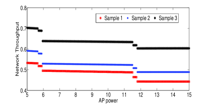
As the power profile space $\mathcal{Q}:=\mathcal{Q}_{1}\times\mathcal{Q}_{2}\times...\times\mathcal{Q}_{N}$ is potentially infinite, and $\mathcal{U}$ is in general a non-convex and non-differentiable function w.r.t. $\mathcal{P}$, the optimization problem is NP-hard. To illustrate, Fig. 1 shows three examples of the sum utility as a function of the power $\mathcal{P}_{i}$ of AP $i$, under different parameter settings. As can be seen, there lack properties commonly used to derive efficient solution techniques (e.g., differentiability, convexity). There are, however, some interesting features such as the prominent step shape shown in the result. This observation motivated key results in the subsequent subsections.

Figure 1: Examples of $\mathcal{U}$ w.r.t. a specific $\mathcal{P}_{i}$

III-D An illustrative example: two-user case with centralized solution

Consider the special case with $N=2$ and $p_{c}=\frac{1}{2}$, i.e., a system of two users attempting to access the channel each with probability 1/2. To gain some insight into the solution to the corresponding optimization problem (P), we discuss the following four cases.

CASE 1. $\mathcal{P}_{1}\leq\mathcal{P}^{-}_{12},\mathcal{P}_{2}\leq\mathcal{P}^{-}_{21}$

In this case neither user is in the other’s CS range and thus the objective function becomes

$$\log(1+\frac{\mathcal{P}_{1}}{\mathcal{N}_{0}+\frac{1}{4}\cdot\mathcal{P}_{2}\cdot h_{21}})+\log(1+\frac{\mathcal{P}_{2}}{\mathcal{N}_{0}+\frac{1}{4}\cdot\mathcal{P}_{1}\cdot h_{12}})$$ (16)

We first fix $\mathcal{P}_{2}$ and analyze the above function w.r.t. $\mathcal{P}_{1}$. Basic algebraic calculation shows that the above objective function is equivalent to (noting $h_{12}=h_{21}$ and denote $h:=\frac{1}{4}\cdot h_{12}=\frac{1}{4}\cdot h_{21}$)

$$\log\left\{1+\frac{1}{\mathcal{N}_{0}+\mathcal{P}_{2}\cdot h}(\mathcal{P}_{1}+\mathcal{P}_{2}/h+\frac{\mathcal{N}_{0}+\mathcal{P}_{2}\cdot h-\mathcal{P}_{2}\cdot\mathcal{N}_{0}/h}{\mathcal{N}_{0}+\mathcal{P}_{1}\cdot h})\right\}$$

Due to the monotonicity of the $\log$ function, the optimization problem is equivalent to maximizing

$$\mathcal{P}_{1}+\mathcal{P}_{2}/h+\frac{\mathcal{N}_{0}+\mathcal{P}_{2}\cdot h-\mathcal{P}_{2}\cdot\mathcal{N}_{0}/h}{\mathcal{N}_{0}+\mathcal{P}_{1}\cdot h}~{}.$$ (17)

If $\mathcal{N}_{0}+\mathcal{P}_{2}\cdot h-\mathcal{P}_{2}\cdot\mathcal{N}_{0}/h<0$, then Eqn. (17) is strictly increasing w.r.t. $\mathcal{P}_{1}$ and thus $\mathcal{P}^{*}_{1}=\mathcal{P}^{-}_{12}$. If $\mathcal{N}_{0}+\mathcal{P}_{2}\cdot h-\mathcal{P}_{2}\cdot\mathcal{N}_{0}/h\geq 0$, then Eqn. (17) is convex and the maximizer is an end point, i.e., $\mathcal{P}^{*}_{1}\in\{\underline{\mathcal{P}}_{1},\mathcal{P}^{-}_{12}\}$. By symmetry we have similar results for user 2.

CASE 2. $\mathcal{P}_{1}\geq\mathcal{P}^{+}_{12},\mathcal{P}_{2}\leq\mathcal{P}^{-}_{21}$

In this case user 1 is in user 2’s receive contention domain, but not the other way round. It follows that the objective function in this case reduces to the following:

$$\log(1+\frac{\mathcal{P}_{1}}{\mathcal{N}_{0}})+\frac{1}{2}\log(1+\frac{\mathcal{P}_{2}}{\mathcal{N}_{0}})$$ (18)

Obviously this function is increasing w.r.t. $\mathcal{P}_{1}$ and $\mathcal{P}_{2}$ and therefore we have $\mathcal{P}^{*}_{1}=\overline{\mathcal{P}}_{1},\mathcal{P}^{*}_{2}=\mathcal{P}^{-}_{21}$.

CASE 3. $\mathcal{P}_{1}\leq\mathcal{P}^{-}_{12},\mathcal{P}_{2}\geq\mathcal{P}^{+}_{21}$

This is essentially the same as CASE 2 and thus omitted.

CASE 4. $\mathcal{P}_{1}\geq\mathcal{P}^{+}_{12},\mathcal{P}_{2}\geq\mathcal{P}^{+}_{21}$

In this case both users are in each other’s contention domain, and the resulting objective function is

$$\frac{1}{2}\log(1+\frac{\mathcal{P}_{1}}{\mathcal{N}_{0}})+\frac{1}{2}\log(1+\frac{\mathcal{P}_{2}}{\mathcal{N}_{0}}).$$ (19)

It is then straightforward to show that $\mathcal{P}^{*}_{1}=\overline{\mathcal{P}}_{1}$ and $\mathcal{P}^{*}_{2}=\overline{\mathcal{P}}_{2}$.

The above example aims at conveying the intuition that the optimal power levels are likely to be at the neighborhood reaching thresholds or the maximum power limit. The next section shows that we can indeed restrict our attention to a finite set of these thresholds in search of an optimal solution.

IV Solution Approach : A centralized View

IV-A A Lower bound problem

Recall that for $j\in\bar{\Delta}^{r}_{i}$, we have $\mathcal{P}_{j}\cdot h_{ji}<\mathcal{P}^{i}_{cs}$, i.e., the received signal strength is below the CS threshold. Thus

$$\log(1 +\frac{\mathcal{P}_{i}}{\mathcal{N}_{0}+\sum_{j\in\bar{\Delta}^{r}_{i}\cap\bar{\Delta}^{t}_{i}}S_{j}(\mathbf{\mathcal{P},\mathbf{p}})\cdot\mathcal{P}_{j}\cdot h_{ji}})$$

$$>\log(1+\frac{\mathcal{P}_{i}}{\mathcal{N}_{0}+\sum_{j\in\bar{\Delta}^{r}_{i}\cap\bar{\Delta}^{t}_{i}}S_{j}(\mathbf{\mathcal{P},\mathbf{p}})\cdot\mathcal{P}^{i}_{cs}})~{}.$$ (20)

We use this relationship to form the following lower bound problem.

$$\begin{array}[]{ccll}\textbf{(PL)}&\max&\mathcal{U}_{L}=\sum_{i\in\Omega}(1-p_{c})^{n_{i}(\mathcal{P})}p_{c}\cdot\\ &{}{}\hfil&~{}~{}\log(1+\frac{\mathcal{P}_{i}}{\mathcal{N}_{0}+\sum_{j\in\bar{\Delta}^{r}_{i}\cap\bar{\Delta}^{t}_{i}}S_{j}(\mathbf{\mathcal{P},\mathbf{p}})\cdot\mathcal{P}^{i}_{cs}})\\ &\text{s.t.}&\mathcal{P}_{i}\in\mathcal{Q}_{i},\forall i\in\Omega.\end{array}$$

Lemma IV.1

For an optimal solution $\mathcal{P}^{*}$ to (PL), we have $\mathcal{P}^{*}\in\tilde{\mathcal{Q}}$. That is, there is no loss of optimality is restricting the solution space to $\tilde{\mathcal{Q}}$ in searching for an optimal solution.

Proof 2

For AP $i$, suppose there exists a $\mathcal{P}^{*}_{i}\not\in\tilde{{\mathcal{Q}}}_{i}$. This means one of the following must be true: (1) $\mathcal{P}^{+}_{ik}<\mathcal{P}^{*}_{i}<\mathcal{P}^{-}_{ij}$ for some $(k,j)$, (2) $\mathcal{P}^{*}_{i}<\mathcal{P}^{-}_{ij}$ for all $j$, and (3) $\mathcal{P}^{+}_{ik}<\mathcal{P}^{*}_{i}$ for all $k$. For the fist two cases, if we increase $\mathcal{P}_{i}$ from $\mathcal{P}^{*}_{i}$ to $\mathcal{P}^{-}_{ij}$, the resulting contention topology remain unchanged, i.e., the terms $\mathcal{S}_{j},n_{j}(\mathcal{P}),\forall j\in\Omega$ stay unchanged, but $\mathcal{P}_{i}$ is now bigger and $\mathcal{U}_{L}$ is strictly increasing in $\mathcal{P}_{i}$. This contradicts the optimality of $\mathbf{\mathcal{P}^{*}}$, so the first two cases cannot be true. If it’s the third case and $\mathcal{P}^{+}_{ik}<\mathcal{P}^{*}_{i}$ for all $k$, then increasing $\mathcal{P}_{i}$ from $\mathcal{P}^{*}_{i}$ to $\overline{\mathcal{P}}_{i}$ results in the same argument as above, so (3) also cannot be true, completing the proof.

Remark IV.2

When $\mathcal{P}^{i}_{cs}$ is small or when the network is dense and large (i.e., with a large $N$), the lower bound problem will provide a good approximation for the original problem.

IV-B An Upper bound problem

We similarly form an upper bound to the original objective function:

$$\log(1 +\frac{\mathcal{P}_{i}}{\mathcal{N}_{0}+\sum_{j\in\bar{\Delta}^{r}_{i}\cap\bar{\Delta}^{t}_{i}}S_{j}(\mathbf{\mathcal{P},\mathbf{p}})\cdot\mathcal{P}_{j}\cdot h_{ji}})$$

$$\leq\frac{\mathcal{P}_{i}}{\mathcal{N}_{0}+\sum_{j\in\bar{\Delta}^{r}_{i}\cap\bar{\Delta}^{t}_{i}}S_{j}(\mathbf{\mathcal{P},\mathbf{p}})\cdot\mathcal{P}_{j}\cdot h_{ji}}\cdot\log 2,$$ (21)

and we have the following upper bound problem

$$\begin{array}[]{ccll}\textbf{(PU)}&\max&\mathcal{U}_{U}=\sum_{i\in\Omega}(1-p_{c})^{n_{i}(\mathcal{P})}p_{c}\\ &&\cdot\frac{\mathcal{P}_{i}}{\mathcal{N}_{0}+\sum_{j\in\bar{\Delta}^{r}_{i}\cap\bar{\Delta}^{t}_{i}}S_{j}(\mathbf{\mathcal{P},\mathbf{p}})\cdot\mathcal{P}_{j}\cdot h_{ji}}\\ &\text{s.t.}&\mathcal{P}_{i}\in\mathcal{Q}_{i},\forall i\in\Omega.\end{array}$$

Lemma IV.3

$\mathcal{U}_{U}$ is piece-wise convex w.r.t. each $\mathcal{P}_{i},i\in\Omega$.

Proof 3

Consider $\mathcal{P}_{i}$ and fix the transmission power of all other APs. Suppose $\mathcal{P}_{i}\in[\mathcal{P}^{+}_{ik},\mathcal{P}^{-}_{ij}]$ for some $k,j$. Within this range, the contention topology remains the same, i.e., $(1-p_{c})^{n_{i}(\mathcal{P})}p_{c}$ is a constant for any value $\mathcal{P}_{i}$ takes within this interval. Next consider the second term in $\mathcal{U}_{U}$. $\mathcal{P}_{i}$ appears in this term in two forms: one as $\frac{\mathcal{P}_{i}}{\mathcal{N}_{0}+\sum_{l\in\bar{\Delta}^{r}_{i}\cap\bar{\Delta}^{t}_{i}}S_{l}(\mathbf{\mathcal{P},\mathbf{p}})\cdot\mathcal{P}_{l}\cdot h_{li}}$ which is convex w.r.t. $\mathcal{P}_{i}$, and the other as $\frac{\mathcal{P}_{l}}{\mathcal{N}_{0}+\sum_{m\in\bar{\Delta}^{r}_{l}\cap\bar{\Delta}^{t}_{l}}S_{m}(\mathbf{\mathcal{P},\mathbf{p}})\cdot\mathcal{P}_{m}\cdot h_{ml}}$ for some $l$ such that $i\in\bar{\Delta}^{r}_{l}\cap\bar{\Delta}^{t}_{l}$, in the form of $S_{i}(\mathbf{\mathcal{P},\mathbf{p}})\cdot\mathcal{P}_{i}\cdot h_{il}$; these terms are also convex w.r.t. $\mathcal{P}_{i}$. As the sum of convex functions is convex, we have established the convexity of $\mathcal{U}_{U}$.

When $\mathcal{P}^{+}_{ik}<\mathcal{P}_{i}$ for all $k$, $\mathcal{U}_{U}$ is convex w.r.t. $\mathcal{P}_{i}$ over the interval $[\max\mathcal{P}^{+}_{ik},\overline{\mathcal{P}}_{i}]$ using the same argument as above. Similarly, when $\mathcal{P}_{i}<P^{-}_{ik},\forall k\neq i$ $\mathcal{U}_{U}$ is convex w.r.t. $\mathcal{P}_{i}$ over the interval $[\underline{\mathcal{P}}_{i},\min\mathcal{P}^{-}_{ik}]$.

Lemma IV.4

Suppose $\mathcal{P}^{*}_{U}$ is the optimal solution to (PU), we have $\mathcal{P}^{*}_{U}\in\tilde{\mathcal{Q}}$.

Proof 4

The result readily follows from Lemma IV.3 and the fact that optimal solution over a closed interval for a convex function is an end point.

Remark IV.5

Since the linear approximation would perform better when $\frac{\mathcal{P}_{i}}{\mathcal{N}_{0}+\sum_{j\in\bar{\Delta}^{r}_{i}\cap\bar{\Delta}^{t}_{i}}S_{j}(\mathbf{\mathcal{P},\mathbf{p}})\cdot\mathcal{P}_{j}\cdot h_{ji}}$ is small, we know when the network size is large (i.e., $N$ is large) and dense, the upper bound problem will provide a good approximation for the original problem.

Remark IV.6

By finding the optimal solution for problems (PL) and (PU), we have the bounds for the optimal solutions.

$$\mathcal{U}_{L}(\mathcal{P}^{*}_{L})\leq\mathcal{U}(\mathcal{P}^{*})\leq\mathcal{U}_{U}(\mathcal{P}^{*}_{U})$$ (22)

Meanwhile we can use $\mathcal{P}^{*}_{L}$ and $\mathcal{P}^{*}_{U}$ as approximate strategies for our original problem (P) with

$$U(\mathcal{P}^{*}_{L})\geq\mathcal{U}_{L}(\mathcal{P}^{*}_{L}),~{}U(\mathcal{P}^{*}_{U})\leq\mathcal{U}_{U}(\mathcal{P}^{*}_{U})$$ (23)

In next section we will focus on solving (PL) and (PU) instead of (P).

IV-C Greedy search

In solving (PL) and (PU) instead of the original (P), the problem reduces to searching over a finite strategy space which can be done within a finite number of steps dependent on the size of the network. For the lower bound problem (PL), the strategy space is on the order of $\mathcal{O}(N^{N})$, while for the upper bound problem (PU) the order is $\mathcal{O}((2N-1)^{N})$. However with a large scale WLAN network (referring to the number of APs in the network), these could still be excessively large even though finite. This is the classical rollout problem in combinatorial optimization. Below we present a heuristic greedy approach, which is shown later through numerical experiment to provide a near-optimal solution efficiently. The basic idea of a greedy search method is to maximize the system’s total throughput w.r.t. a single variable at each stage of the computation while keeping the others fixed. The details of this approach is shown in Algorithm 1, where the notation $\mathcal{P}_{-m}$ denotes the power profile for all but AP $m$, and the objective function ${\mathcal{U}}()$ denote either $\mathcal{U}_{U}$ or $\mathcal{U}_{L}$ depending on which problem ((PU) vs. (PL)) we are trying to solve.

 

  Set $\mathcal{P}_{i}(0)=\overline{\mathcal{P}}_{i},\forall i\in\Omega$.

  $\text{temp}=\mathcal{U}(\mathcal{P}(0))$, $\epsilon=\text{temp}$, $n=0$.

while $\epsilon>0$ do

  $n:=n+1$;

  $m:=n\mod N$;

  $\mathcal{P}_{m}(n)=\operatorname{argmax}_{\mathcal{P}^{m}\in\tilde{\mathcal{Q}}_{m}}\mathcal{U}(\mathcal{P}^{m},\mathcal{P}_{-m}(n-1))$;

  for $j=1:N$ do

           if $j\neq m$

              $\mathcal{P}_{j}(n)=\mathcal{P}_{j}(n-1)$;

  end for

        $\epsilon=|\mathcal{U}(\mathcal{P}(n))-\text{temp}|$;

        $\text{temp}=\mathcal{U}(\mathcal{P}(n))$;

      

end while

 

Algorithm 1 Pseudocode for Greedy Search

Lemma IV.7

The above greedy search terminates within a finite number of steps and reaches a local optimal solution to (PL) and (PU).

IV-D Optimal search

In this part, we present a randomized search algorithm that guarantees convergence to the optimal solution for (PL) and (PU). The algorithm works in rounds starting from AP $1$ and computes the power for one AP in each round. Denote the state of the system at round $n$ as $\mathcal{G}(n)$ and $\mathcal{G}(n):=[\mathcal{P}_{1}(n),\mathcal{P}_{2}(n),...,\mathcal{P}_{N}(n)]$. Suppose at round $n$ AP $i$’s (i.e., $i=n\mod N$) power is being computed. Then AP $i$’s next power level is updated using the following transition probability:

$$\mathbb{P}(\mathcal{G}(n+1)=(\mathcal{P}^{i},\mathcal{G}_{-i}(n))|\mathcal{G}(n))$$

$$=\frac{e^{\mathcal{U}(\mathcal{P}^{i},\mathcal{G}_{-i}(n))/\tau(n)}}{e^{\mathcal{U}(\mathcal{P}^{i},\mathcal{G}_{-i}(n))/\tau(n)}+e^{\mathcal{U}(\mathcal{G}(n))/\tau(n)}}\cdot\frac{1}{\mathcal{L}_{i}},$$

$$~{}\forall\mathcal{P}^{i}\in\tilde{\mathcal{Q}}_{i},\mathcal{P}^{i}\neq\mathcal{P}_{i}(n).$$ (24)

with the probability of not changing the power level given as

$$~{}~{}~{}~{}~{}~{}\mathbb{P}(\mathcal{G}(n+1)=\mathcal{G}(n)|\mathcal{G}(n))$$

$$=\sum_{\mathcal{P}^{i}\in\tilde{\mathcal{Q}}_{i},\mathcal{P}^{i}\neq\mathcal{P}_{i}(n)}\frac{e^{\mathcal{U}(\mathcal{G}(n))/\tau(n)}}{e^{\mathcal{U}(\mathcal{P}^{i},\mathcal{G}_{-i}(n))/\tau(n)}+e^{\mathcal{U}(\mathcal{G}(n))/\tau(n)}}\cdot\frac{1}{\mathcal{L}_{i}}~{}.$$ (25)

Here $\tau(n):=\frac{1}{n}$ is a positive smoothing factor and $\mathcal{L}_{i}$ is a normalization factor for user $i$. This search algorithm will be referred to as P_RAND. As before, the function ${\mathcal{U}}()$ in the above equation is the objective in problem (PL) (resp. (PU)) if the algorithm is used to search for an optimal solution to problem (PL) (resp. (PU)).

 

  Set $\mathcal{P}_{i}(0)=\overline{\mathcal{P}}_{i},\forall i\in\Omega$.

  $\text{temp}=\mathcal{U}(\mathcal{P}(0))$, $\epsilon=\text{temp}$, $n=0$.

  $\text{thrs}=10^{-4}$. (some small positive value)

while $\epsilon>\text{thrs}$ do

  $n:=n+1$ ;

  $m:=n\mod N$;

  Set $\mathcal{P}_{m}(n)=\mathcal{P}^{m}$ with probability $\frac{e^{\mathcal{U}(\mathcal{P}^{m},\mathcal{G}_{-m}(n))/\tau(n)}}{e^{\mathcal{U}(\mathcal{P}^{m},\mathcal{G}_{-m}(n))/\tau(n)}+e^{\mathcal{U}(\mathcal{G}(n))/\tau(n)}}\cdot\frac{1}{\mathcal{L}_{m}},\forall\mathcal{P}^{m}\in\tilde{\mathcal{Q}}_{m},\mathcal{P}^{m}\neq\mathcal{P}_{m}(n)$.

  While $\mathcal{P}_{m}(n)$ stays unchanged with probability $\sum_{\mathcal{P}^{m}\in\tilde{\mathcal{Q}}_{i},\mathcal{P}^{m}\neq\mathcal{P}_{m}(n)}\frac{e^{\mathcal{U}(\mathcal{G}(n))/\tau(n)}}{e^{\mathcal{U}(\mathcal{P}^{m},\mathcal{G}_{-i}(n))/\tau(n)}+e^{\mathcal{U}(\mathcal{G}(n))/\tau(n)}}\cdot\frac{1}{\mathcal{L}_{m}}$.

  for $j=1:N$ do

           if $j\neq m$

              $\mathcal{P}_{j}(n)=\mathcal{P}_{j}(n-1)$;

  end for

        $\epsilon=|\mathcal{U}(\mathcal{P}(n))-\text{temp}|$;

        $\text{temp}=\mathcal{U}(\mathcal{P}(n))$;

      

end while

 

Algorithm 2 Pseudocode for Randomized Search

Theorem IV.8

P_RAND converges to the optimal solution to the two approximate problems (PL) and (PU).

Proof 5

Due to the finiteness of the strategy spaces of all APs, we can form an $N$-dimensional positive recurrent Markov chain, with state at time $n$ given by $\mathcal{G}(n)$; there exists a stationary distribution of this Markov chain.

We next show that the following probability distribution $\pi$ over the state space $\tilde{\mathcal{Q}}$ is the stationary distribution of this Markov Chain.

$$\pi(\mathcal{G})=T\cdot e^{\mathcal{U}(\mathcal{G})/\tau(n)},\forall\mathcal{G}\in\tilde{\mathcal{Q}}~{},$$ (26)

where $T$ is the normalization constant. As $\sum_{\mathcal{G}\in\tilde{\mathcal{Q}}}\pi(\mathcal{G})=1$ the above is equivalent to $T=\sum_{\mathcal{G}\in\tilde{\mathcal{Q}}}e^{\mathcal{U}(\mathcal{G})/\tau(n)}~{},$ and thus

$$\pi(\mathcal{G})=\frac{e^{\mathcal{U}(\mathcal{G})/\tau(n)}}{\sum_{\mathcal{G}\in\tilde{\mathcal{Q}}}e^{\mathcal{U}(\mathcal{G})/\tau(n)}},\forall\mathcal{G}\in\tilde{\mathcal{Q}}~{},$$ (27)

To prove this, consider the detailed balance equations. Specifically consider two states $\mathcal{G}_{1}$ and $\mathcal{G}_{2}$. Note that only when $\mathcal{G}_{1}$ and $\mathcal{G}_{2}$ differ in one element is the transition probability is positive; otherwise the transition probability is zero. We would like to show the following

$$\pi(\mathcal{G}_{1})\cdot\mathbb{P}(\mathcal{G}_{2}|\mathcal{G}_{1})=\pi(\mathcal{G}_{2})\cdot\mathbb{P}(\mathcal{G}_{1}|\mathcal{G}_{2}),\forall\mathcal{G}_{1},\mathcal{G}_{2}.$$ (28)

When there is only one element difference between the two states we know

$$\mathbb{P}(\mathcal{G}_{2}|\mathcal{G}_{1})=\mathcal{L}\cdot\frac{e^{\mathcal{U}(\mathcal{G}_{2}/\tau(n))}}{e^{\mathcal{U}(\mathcal{G}_{2}/\tau(n))}+e^{\mathcal{U}(\mathcal{G}_{1}/\tau(n))}}$$ (29)

$$\mathbb{P}(\mathcal{G}_{1}|\mathcal{G}_{2})=\mathcal{L}\cdot\frac{e^{\mathcal{U}(\mathcal{G}_{1}/\tau(n))}}{e^{\mathcal{U}(\mathcal{G}_{1}/\tau(n))}+e^{\mathcal{U}(\mathcal{G}_{2}/\tau(n))}}$$ (30)

with $\mathcal{L}$ being some constant. Therefore (28) holds readily. It follows from standard result that $\pi$ is indeed the stationary distribution.

Denote $\mathcal{G}^{*}=\{\mathcal{P}^{*}\}$ as the set of global maximizers; i.e., the set of power profiles that maximizes our objectives in (PL) and (PU) respectively. Suppose there is a state $\mathcal{G}^{{}^{\prime}}\notin\mathcal{G}^{*}$. We have

$$\pi(\mathcal{G}^{{}^{\prime}})= \frac{e^{\mathcal{U}(\mathcal{G}^{{}^{\prime}})/\tau(n)}}{\sum_{\mathcal{G}\in\tilde{\mathcal{Q}}}e^{\mathcal{U}(\mathcal{G})/\tau(n)}}=\frac{1}{\sum_{\mathcal{G}\in\tilde{\mathcal{Q}}}e^{(\mathcal{U}(\mathcal{G})-\mathcal{U}(\mathcal{G}^{{}^{\prime}}))/\tau(n)}}$$ (31)

For $\mathcal{G}\in\mathcal{G}^{*}$ we have $\mathcal{U}(\mathcal{G})-\mathcal{U}(\mathcal{G}^{{}^{\prime}})>0$ and

$$\lim_{n\rightarrow\infty}(\mathcal{U}(\mathcal{G})-\mathcal{U}(\mathcal{G}^{{}^{\prime}}))/\tau(n)\rightarrow\infty$$ (32)

and hence we have $\lim_{n\rightarrow\infty}\pi(\mathcal{G}^{{}^{\prime}})=0$ ; furthermore by [1] we establish the following

$$\lim_{n\rightarrow\infty}\pi(\mathcal{G}\in\mathcal{G}^{*})=1$$ (33)

i.e., the Markovian chain converges to the maximization states with probability 1.

V Solution Approach : A decentralized View

V-A A game theoretic view

Starting from this section we analyze a strategic network for our problem. We first form a game theoretical model. Instead of group of users sharing a common goal, we assume the network users being strategic, i.e. with each one being rational. Define $\Delta\mathcal{Q}:=\Delta\mathcal{Q}_{1}\times\Delta\mathcal{Q}_{2}\times...\Delta\mathcal{Q}_{N}$. Here $\Delta\mathcal{Q}_{i}$ is the probability measure over action space $Q_{i}$. Then $(\Omega,\Delta\mathcal{Q}_{i},\mathcal{U}_{i})$ defines our game. We call this game (G1). We investigate the Nash Equilibrium (N.E.) of above game. To be specific, we show there is one unique N.E. exists for above game.

Proposition V.1

The only N.E. for (G1) is $\mathbf{\overline{\mathcal{P}}}=[\overline{\mathcal{P}}_{1},\overline{\mathcal{P}}_{2},...,\overline{\mathcal{P}}_{N}]$.

Proof 6

First we show $\mathbf{\overline{\mathcal{P}}}$ is a N.E.. Without of losing generality, consider AP $i$. As $\mathcal{S}_{i}(\mathbf{\mathcal{P}},\mathbf{p})$ is independent with $\mathcal{P}_{i}$ and $\mathcal{C}_{i}$ is a strictly increasing function w.r.t. $\mathcal{P}_{i}$, by unilaterally deviating from $\overline{\mathcal{P}}_{i}$ to some lower power profile $\mathcal{P}^{{}^{\prime}}_{i}$, $\mathcal{U}_{i}$ will decrease. Therefore we proved $\mathbf{\overline{\mathcal{P}}}$ is a N.E.. From above arguments we also established the uniqueness immediately.

V-B Mechanism design with perfect monitoring

Starting from this part we solve our problem with mechanism design’s approach. First of all since we are more interested in a dense network with well interacted APs we make the following assumption: for each user $i$, there is at least one $j$ such that

$$\overline{\mathcal{P}}_{j}\cdot h_{ji}\geq\mathcal{P}^{i}_{cs}$$ (34)

i.e., for any AP it can be reached by at least one another AP within its carrier sensing range. Consider the case where there is such AP that nobody can reach him and let’s call it a stand-alone AP. This AP can be thought of disconnected from the network and it cannot be controlled by the other APs’ behaviors; or in a homogeneous network, this stand-alone AP will not contribute to other people’s utility in a significant way and thus we could screen this case out and focus on the rest well connected APs.

We first start with the mechanism design problem with perfect monitoring; here by perfect monitoring we mean each user can monitor other users’ transmission power in a perfect way without noise. As we discussed in last section, the socially optimal power allocation strategy profile may not be a NE of the multiuser system. Meanwhile, it is easy to check each user’s utility function is a strictly increasing function w.r.t. the attempt rate $p$. Therefore in a decentralized system, each user has two incentives to deviate from our socially optimal strategy profile:

• Deviate from pre-specified transmission power to get a higher SNR.

• Deviate from $p_{c}$ to get more air time.

In this section we consider the optimization problem from a long run perspective for each user, i.e., we consider the following programming problem

$$\begin{array}[]{ccll}(P^{*}_{i})&\max&\sum_{t=0}^{\infty}\delta^{t}\cdot\mathcal{U}_{i}(\mathbf{\mathcal{P}}(t),\mathbf{p}(t))\\ &\text{s.t.}&\mathcal{P}_{i}(t)\in\mathcal{Q}_{i},\forall i\in\Omega,t=0,1,2,...\end{array}$$

Here $\delta$ is the discount factor satisfying $0<\delta<1$ and it models users or system’s patience. Denote the social optimal power setting as $\mathbf{(\mathcal{P}^{*},p)}$. We define the following states of APs:

• $S_{0}$: The initial state; at $S_{0}$ the group of APs follow the strategy profile $\mathbf{(\mathcal{P}^{*},p)}$.

• $S_{i}(t),t=1,2,...,L,i\in\Omega$: Punishment phases for user $i$. At state $S_{i}(t)$ APs follow the specified strategy profile $\mathbf{(\overline{\mathcal{P}}},(\tilde{p}_{i},[\tilde{p}_{ji}]_{j\neq i}))$. Here $L$ is some finite positive integer which is the length of punishment phases.

Consider the following mechanism.

• APs start at state $S_{0}$. If all APs follow the strategy profile $\mathbf{(\mathcal{P}^{*},p)}$ specified for $S_{0}$, at next time APs will keep playing the strategy profile.

• If there is one AP, for example $i$ deviated from $\mathbf{(\mathcal{P}^{*},p)}$ at time $t$, starting from time $t+1$, system goes into state $S_{i}(1)$ and play strategy profile $\mathbf{(\overline{\mathcal{P}}},(\tilde{p}_{i},[\tilde{p}_{ji}]_{j\neq i})$.

• At state $S_{i}(t),t=1,2,...,L-1$, if all APs follow the specified strategy, system goes to state $S_{i}(t+1)$ at next time point; at $S_{i}(L)$, if all APs follow the specified strategy, system goes to state $S_{0}$.

• At state $S_{i}(t),t=1,2,...,L$, if AP $i$ deviates from the specified strategy profile, system goes to state $S_{i}(1)$ at next time. If AP $j\neq i$ deviates, system goes to $S_{j}(1)$.

We refer this mechanism as (MPM). Now we present some requirements on choosing over $([\tilde{p}_{i}]_{i\in\Omega},[\tilde{p}_{j,k}]_{j\neq k})$.

• $[\tilde{p}_{ji}]_{j\neq i}$ should be large enough to deter user $i$. Notice that with large enough $[\tilde{p}_{ji}]_{j\neq i}$ (with each elements close enough to 1) we have

  $$\mathcal{S}_{i}(\overline{\mathcal{P}},\tilde{p}_{i},[\tilde{p}_{ji}]_{j\neq i})\rightarrow 0,\mathcal{U}_{i}(\overline{\mathcal{P}},\tilde{p}_{i},[\tilde{p}_{ji}]_{j\neq i})\rightarrow 0$$ (35)

  This essentially follows the intuition that when some user else becomes excessively aggressive, AP $i$ will lose most of its airtime (throttled by other users) and thus results a significant decrease of its achievable throughput. Therefore with appropriately chosen parameter set $\tilde{\mathbf{p}}$ we can get

  $$\mathcal{U}_{i}\mathbf{(\overline{\mathcal{P}}},\tilde{p}_{i},[\tilde{p}_{ji}]_{j\neq i})<\mathcal{U}_{i}\mathbf{(\mathcal{P}^{*},p)}$$ (36)

• A second restriction over selecting $([\tilde{p}_{i}]_{i\in\Omega},[\tilde{p}_{j,k}]_{j\neq k})$ is that each AP $i$ would like to stay at other users’ punishment phase instead of its own, i.e.,

  $$\mathcal{U}_{i}\mathbf{(\overline{\mathcal{P}}},\tilde{p}_{j},[\tilde{p}_{kj}]_{k\neq j})\geq\mathcal{U}_{i}\mathbf{(\overline{\mathcal{P}}},\tilde{p}_{i},[\tilde{p}_{ki}]_{k\neq i})$$ (37)

  Through simple algebra we can show the existence of such strategy profiles w.r.t. APs’ attempt rate. The details are thus omitted here.

• A third restriction on selecting $([\tilde{p}_{i}]_{i\in\Omega},[\tilde{p}_{j,k}]_{j\neq k})$ we put is as following.

  $$\mathcal{U}_{i}(\overline{\mathcal{P}}, p_{i}=1,[\tilde{p}_{ji}]_{j\neq i})-\mathcal{U}_{i}(\overline{\mathcal{P}},\tilde{p}_{i},[\tilde{p}_{ji}]_{j\neq i})$$

  $$<\mathcal{U}_{i}(\overline{\mathcal{P}},\mathbf{p})-\mathcal{U}_{i}(\overline{\mathcal{P}},\tilde{p}_{i},[\tilde{p}_{ji}]_{j\neq i})$$ (38)

  i.e., $[\tilde{p}_{i}]_{i}$ is large enough. We will discuss the intuition later.

Remark V.2

It can be shown a trivial combination for such $([\tilde{p}_{i}]_{i\in\Omega},[\tilde{p}_{j,k}]_{j\neq k})$ is setting each element to be 1, i.e., $([\tilde{p}_{i}]_{i\in\Omega},[\tilde{p}_{j,k}]_{j\neq k})=\mathbf{1}$. Here $\mathbf{1}$ is the all-one vector with corresponding length. However we do not want these punishments to be too harsh and these three requirements help establish our mechanism while keep the punishments as light as possible.

Now we show with appropriately chosen parameter, (MPM) enforces the strategy profile $\boldsymbol{(\mathcal{P}^{*},p)}$ for all APs.

Theorem V.3

$\boldsymbol{(\mathcal{P}^{*},p)}$ is enforceable under mechanism (MPM) with large enough $\delta$ and appropriately chosen $L$.

Proof 7

To prove the enforceability of $\boldsymbol{(\mathcal{P}^{*},p)}$ we need to check no AP would like to go for a one step deviation at any state of (MPM) (according to the one step deviation principle ).

First check state $S_{0}$. Consider an arbitrary AP $i$. Denote the utility from following the social optimal strategy profile for AP $i$ as $\mathcal{U}^{*}_{i}$. Then by following the specified strategy at $S_{0}$, the long run accumulated utility for AP $i$ is given by

$$\mathcal{U}_{i}(S_{0}) =\delta^{0}\cdot\mathcal{U}^{*}_{i}+...+\delta^{t}\cdot\mathcal{U}^{*}_{i}+...=\frac{1}{1-\delta}\mathcal{U}^{*}_{i}$$ (39)

Next check the utility for AP $i$ by deviating to another profile $(\mathcal{P}^{{}^{\prime}}_{i},p^{{}^{\prime}}_{i})$. Remember due to the finiteness of $\mathcal{Q}_{i}$ and $p$ ($0<p<1$), we have some finite positive number $M_{i}$ such that

$$\mathcal{U}_{i}((\mathcal{P}^{{}^{\prime}}_{i},p^{{}^{\prime}}_{i}),\mathbf{(\mathcal{P},p)}_{-i})\leq M_{i}$$ (40)

Also denote the utility of AP $i$ of adopting $\mathbf{(\overline{\mathcal{P}}},\tilde{p}_{i},[\tilde{p}_{ji}]_{j\neq i})$ at punishment phase $S_{i}(t)$ as $\mathcal{U}^{p}_{i}$. Then by deviation we know the aggregated utility for AP $i$ is

$$\mathcal{U}^{d}_{i}(S_{0})\leq M_{i}+\delta\cdot\mathcal{U}^{p}_{i}+\delta^{2}\cdot\mathcal{U}^{p}_{i}+...$$

$$+\delta^{L}\cdot\mathcal{U}^{p}_{i}+\delta^{L+1}\cdot\mathcal{U}^{*}_{i}+...$$ (41)

Then we have

$$\mathcal{U}_{i}(S_{0})-\mathcal{U}^{d}_{i}(S_{0})\geq(\mathcal{U}^{*}_{i}-M_{i})+(\mathcal{U}^{*}_{i}-\mathcal{U}^{p}_{i})\cdot\frac{\delta-\delta^{L+1}}{1-\delta}$$ (42)

As $\mathcal{U}^{*}_{i}-M_{i}\leq 0,\mathcal{U}^{*}_{i}-\mathcal{U}^{p}_{i}>0$, with a large enough $\delta$ and $L$ we could have

$$\frac{\delta-\delta^{L+1}}{1-\delta}\rightarrow L,~{}(\mathcal{U}^{*}_{i}-\mathcal{U}^{p}_{i})\cdot L \geq M_{i}-\mathcal{U}^{*}_{i}$$ (43)

Denote a pair of suitable $(\delta,L)$ as $(\delta^{1},L^{1})$ and we proved with $(\delta^{1},L^{1})$ there will be no profitable one step deviation for any AP at state $S_{0}$.

Next we analyze the punishment phases. Consider $S_{i}(t)$. First notice that obviously all APs at any punishment phase with any stage $S_{j}(t),\forall j\in\Omega,t=1,2,...,L$ there is no incentive to deviate their power strategy. This follows from the observation each AP $i$’s utility $\mathcal{U}_{i}$ is strictly increasing w.r.t. $\mathcal{P}_{i}$. Thus no user would deviate from their maximum transmission power as used in the specified strategy profile at $S_{j}(t)$. Therefore we only need to consider APs deviating with attempt rate $\mathbf{p}$.

First consider AP $i$. Denote $\mathcal{U}_{i}(S_{i})$ as the utility AP $i$ can get by following $S_{i}$. By increasing its attempt rate, AP $i$ will increase its utility. But again due to the finiteness of $p_{i}$ we have a upper bound for this one step increase and we denote it as $M^{{}^{\prime}}_{i}$. Then suppose at stage $t$, AP $i$’s utility by following specified strategy is given by

$$\mathcal{U}_{i}(S_{i}(t))= \mathcal{U}_{i}(S_{i})+\delta\cdot\mathcal{U}_{i}(S_{i})+...$$

$$+\delta^{L-t-1}\mathcal{U}_{i}(S_{i})+\delta^{L-t}\mathcal{U}_{i}(S_{0})+...$$ (44)

and by deviating we have

$$\mathcal{U}^{d}_{i}(S_{i}(t))\leq M^{{}^{\prime}}_{i}+\delta\cdot\mathcal{U}_{i}(S_{i})+...$$

$$+\delta^{L}\mathcal{U}_{i}(S_{i})+\delta^{L+1}\mathcal{U}_{i}(S_{0})+...$$ (45)

Then take the difference we have

$$\mathcal{U}_{i}(S_{i}(t))-\mathcal{U}^{d}_{i}(S_{i}(t))$$

$$\geq\mathcal{U}_{i}(S_{i})-M^{{}^{\prime}}_{i}+\delta\cdot(\mathcal{U}_{i}(\mathcal{P})-\mathcal{U}_{i}(S_{i}))$$ (46)

As $0<M^{{}^{\prime}}_{i}-U_{i}(S_{i})<\mathcal{U}_{i}(\mathcal{P})-\mathcal{U}_{i}(S_{i})$ and with a large enough $\delta$ we have $\mathcal{U}_{i}(S_{i})-M^{{}^{\prime}}_{i}+\delta\cdot(\mathcal{U}_{i}(\mathcal{P})-\mathcal{U}_{i}(S_{i}))>0$.

The last step is to check whether AP $j\neq i$ would deviate at state $S_{i}(t)$ or not. As we already put constraints on $([\tilde{p}_{i}]_{i\in\Omega},[\tilde{p}_{j,k}]_{j\neq k})$ such that each player would rather stay at other AP’s punishment phase instead of their own, hereby AP $j$ would not deviate.

V-C Mechanism design with imperfect monitoring

In this subsection we analyze the problem that each user has imperfect monitoring over other users’ transmission power at each decision period. In practice, the monitoring over other APs’ deviation cannot be done in real time dues to multiple sources of noises, e.g., thermal noise. Therefore without a central monitor, each user needs to precisely detect a deviation by its own observations.

To be specific we consider the following noise model : Instead of being $\mathcal{P}_{j}\cdot h_{ji}$, the received power at user $i$ (transmitted from user $j$) is given by

$$\mathcal{P}_{j}\cdot h_{ji}+\mathcal{N}_{i}$$ (47)

here $\mathcal{N}_{i}$ is a noise source at user $i$’s receiver side which follows a Gaussian distribution, $\mathcal{N}_{i}\sim\mathcal{N}(0,\sigma_{i})$. Moreover we assume any pair $(\mathcal{N}_{i},\mathcal{N}_{j}),i,j\in\Omega$ are correlated with correlation matrix $\Sigma_{ij}$:

$$\Sigma_{ij}=\left[\begin{array}[]{ccc}\sigma_{ii}&\sigma_{ij}\\ \sigma_{ji}&\sigma_{jj}\end{array}\right].$$

For each user we propose the following mechanism. Each user takes a threshold $\epsilon_{i}$ for detection. If $|\mathcal{P}_{ji}-\mathcal{P}_{j}\cdot h_{ji}|\leq\epsilon_{i}$, user $i$ will hold the punishment while taking the user $j$ being non-deviating. On the other hand if $|\mathcal{P}_{ji}-\mathcal{P}_{j}\cdot h_{ji}|>\epsilon_{i}$, user $i$ will initialize the punishment phase for user $j$. Therefore we have

$$\mathbb{P}^{n}_{ij}=\mathbb{P}(|\mathcal{P}_{ji}-\mathcal{P}_{j}\cdot h_{ji}|\leq\epsilon_{i})=2\Phi_{i}(\epsilon_{i})-1$$ (48)

$$\mathbb{P}^{p}_{ij}=1-\mathbb{P}(|\mathcal{P}_{ji}-\mathcal{P}_{j}\cdot h_{ji}|\leq\epsilon_{i})=2-2\Phi_{i}(\epsilon_{i})$$ (49)

Here $\mathbb{P}^{n}_{ij}$ is the probability of detecting no deviation while $\mathbb{P}^{p}_{ij}$ is the probability of positive detection. We name this mechanism (MIM); and similarly with (MPM) we have enforceability as following.

Theorem V.4

$\boldsymbol{(\mathcal{P}^{*},p)}$ is enforceable under mechanism (MIM) with large enough $\delta$, appropriately chosen $L$ and positive correlated noise sources.

Proof 8

To see this threshold based detection strategy is enforceable, we need to show:

• User $i$ would like to adopt the threshold based detection strategy.

• User will not take advantage of this threshold based strategy of other users.

For I, we can design a similar punishment phases and punishment strategies to deter users from deviating from the pre-specified strategy.

Lemma V.5

Users will not deviate from the pre-specified threshold strategy.

Proof 9

Denote the event user $i$ detects a deviation as $E_{i}$ and the event for no detection triggered as $\bar{E}_{i}$. We make the following assumptions over $\Sigma_{ij}$ so that

$$\mathbb{P}(E_{i}|E_{j})>\mathbb{P}(\bar{E}_{i}|E_{j}),\mathbb{P}(E_{j}|E_{i})>\mathbb{P}(\bar{E}_{j}|E_{i})$$ (50)

Or equivalently $\mathbb{P}(E_{i}|E_{j})>\frac{1}{2},\forall i,j\in\Omega$; and we call the noise sources are positively correlated with each other. We show an example as following to demonstrate what kinds of noise resources have positive correlation.

Example 1

. Bi-variate Gaussian Distribution

Consider

$$\Sigma_{ij}=\left[\begin{array}[]{ccc}1&\rho_{ij}\\ \rho_{ij}&1\end{array}\right].$$

The sufficient condition for a positive correlation is given as (algebraic details omitted for concise presentation)

$$\Phi(\frac{\epsilon_{i}-\sqrt{\rho_{ij}}\epsilon_{j}}{\sqrt{1-\rho^{2}_{ij}}})+\Phi(\frac{\epsilon_{i}+\sqrt{\rho_{ij}}\epsilon_{j}}{\sqrt{1-\rho^{2}_{ij}}})>1+\frac{1}{2}$$ (51)

Following which a more loose condition comes as

$$\Phi(\epsilon\cdot\frac{1-\sqrt{\rho_{ij}}}{\sqrt{1-\rho_{ij}^{2}}})>\frac{3}{4}$$ (52)

Therefore following right after Equation (52) a simple and sufficient condition for the positive correlation is

$$\epsilon_{i}=\epsilon_{j},\rho_{ij}\rightarrow 1$$ (53)

and $\epsilon_{i},i\in\Omega$ are properly chosen. The results show that in a network with homogeneous noise sources we need the correlation factor to be high enough. This follows the intuition of designing deviation-proof mechanisms for private imperfect monitoring problems: only when the correlation of private observations are highly positive correlated.

Therefore when a user deviates, the probability of being detected by other users becomes higher than sticking with prescribed strategy. As long as we have a harsh and long enough punishment phase for each users, nobody will deviate. The design details follow similar path with (MIM) as in the perfect monitoring section and thus omitted.

Now we consider II and particularly we would like to see nobody could be able to take use of the “cushion” tolerance of other users by the threshold policy.

Lemma V.6

No user will deviate to take use of the threshold detection strategy of other users.

Proof 10

Without losing generality, consider user $i$. Suppose user $i$ increase $\mathcal{P}^{*}_{i}$ to $\mathcal{P}^{*}_{i}+\tau$. Denote the benefits of the deviation for user $i$ as $\Delta~{}\mathcal{U}_{i}(\tau)$. Firstly with the change, at user $j\neq i$’s side, the probability of punishment initialized becomes

$$\mathbb{P}^{p,\tau}_{ji} =1-\mathbb{P}(-\epsilon_{j}\leq\mathcal{N}_{j}+\tau\cdot h_{ij}\leq\epsilon_{j})$$

$$=2-(\Phi_{j}(\epsilon_{j}+\tau\cdot h_{ij})+\Phi_{j}(\epsilon_{j}-\tau\cdot h_{ij}))$$ (54)

By basic algebra we can show (details omitted)

$$2-(\Phi_{j}(\epsilon_{j}+\tau\cdot h_{ij}) +\Phi_{j}(\epsilon_{j}-\tau\cdot h_{ij}))$$

$$>2-2\cdot\Phi_{j}(\epsilon_{j})$$ (55)

i.e., $\mathbb{P}^{p,\tau}_{ji}>\mathbb{P}^{p}_{ji}$; and furthermore we have $\frac{\partial(\mathbb{P}^{p,\tau}_{ji}-\mathbb{P}^{p}_{ji})}{\partial\epsilon_{j}}<0$. The intuition here is when $\epsilon_{j}$ is smaller, user $i$ would be detected with transmit power change $\tau$ more easily. Therefore by designing appropriate detection thresholds $\epsilon_{j},j\in\Omega$ and punishment phases with large enough $\delta$ and $L$ we have the following

$$(\mathbb{P}^{p,\tau}-\mathbb{P}^{p})\{ \underbrace{(\mathcal{U}^{*}_{i}-\mathcal{U}^{p}_{i})+\delta(\mathcal{U}^{*}_{i}-\mathcal{U}^{p}_{i})+...+\delta^{L-1}(\mathcal{U}^{*}_{i}-\mathcal{U}^{p}_{i})}_{L}\}$$

$$>\Delta~{}\mathcal{U}_{i}(\epsilon)$$ (56)

Therefore each user would be deterred from deviating under this threshold enabled detection mechanism.

Theorem V.7

The (MIM) help increases system performance compared with (MPM) under a imperfect monitoring system.

Proof 11

We sketch the basic idea here. Obviously by introducing in the $\epsilon$ tolerance threshold we decreased the false alarm probability. As the network performance degradation caused by punishment is more severe than the degradation by the other users’ slight deviation (light deviation under tolerance) or by the noise, we know the (MIM) helps improve system performance.

VI Numerical Experiments

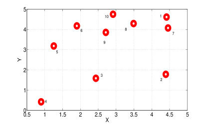
In this section, we provide simulation results to show system performance under the greedy and randomized search algorithms (denoted as “Greedy” and “P_RAND” in the figures, respectively). We further compare them with the maximum transmission power strategy (“Max”), PPHY and PMAC respectively. The WLAN network’s topology used in the experiment is randomly generated, with 10 APs placed according to a uniform distribution in a square area; this topology is shown in Fig.2.

Figure 2: Topology of the AP Network

VI-A Optimization with dual effects

We begin by comparing the computed power levels and the resulting system-wide throughput under the greedy and randomized search algorithms and the fixed, maximum power scheme.

Figure 3: Output power levels under Greedy Search & P_RAND.

Figure 4: Comparison of system-wide throughput.

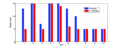
For the first set of results, we fix $p_{c}=0.6$ and a maximum transmission power level of 15 for all APs. The resulting optimal power profile is depicted in Fig.3. Here to get the “optimal solution” we utilize P_RAND to solve (PL) and (PU) separately and then choose the one that gives us a better total throughput. We see that in this case APs $(8,9,10)$’s power levels are far short of the maximum level. This reflects the need to avoid excessive interference with each other as they are clustered in a relatively crowded neighborhood. APs $(2,4)$ are sitting relatively “alone” and thus they could transmit at a higher power. Similar observations can be made at each AP.

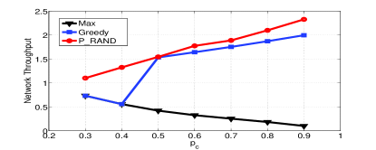
Next, the system performance is shown in Fig. 4 as a function of the attempt rate $p_{c}$. It is interesting to note the opposite trends exhibited by using optimal power tuning vs. always using maximum power levels as the attempt rate increases. As the network gets busier (more congested with higher attempt rate), the maximum power levels exacerbates the problem and the system throughput degrades even though the APs are trying harder. On the other hand, using optimal power-tune, as the network becomes more congested, the APs react by decreasing their transmission powers appropriately so that the system throughput actually improves. By either the greedy search or the randomized search algorithm, our optimal power-tune problem helps achieve a significant throughput performance improvement compared to the static maximum transmission power scheme.

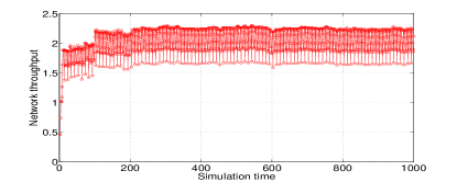
We end this part with a look into the convergence performance of P_RAND, shown in Fig.5. It is seen that our randomized search algorithm converges quickly to the end solution; under the same simulation setting, the greedy policy converges to a solution of system throughput at around 1.6.

Figure 5: Convergence of P_RAND

VI-B Compare with PPHY

We next compare our optimization model with dual effect to the model given by PPHY, which tries to maximize the total rate at the physical layer without considering contention. The achievable throughput at each AP node (under attempt rate $p_{c}=0.6$ ) is shown in Fig. 6 while the transmission power returned by PPHY vs. that by P_RAND is shown in Fig. 7.

Figure 6: AP’s individual throughput

Figure 7: power-tune results

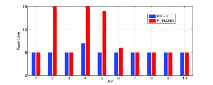
We see a clear difference in how power levels are tuned and the resulting throughput across different AP nodes. The reason is that under PPHY each AP treats all other APs as noise resources. However, due to CSMA/CA, no parallel transmission would be allowed for APs within the carrier sensing range and thus the first-order noises (those from the closest neighbors) could be removed. Therefore APs could increase their power to some extent without contributing too much to their neighbors’ noise level. This is why we observe a few APs with much higher power under P_RAND than under PPHY. By contrast, with only PHY layer optimization APs cannot take full advantages of the noise-free property of CSMA, and therefore act conservatively.

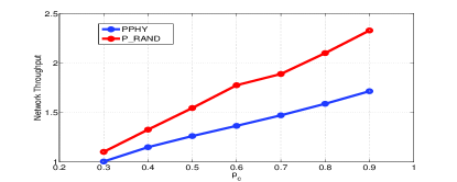
To make our comparison complete we present the total system throughput performance in Fig. 8. We see PPHY is clearly out-performed by our optimization model especially under higher attempt rate.

Figure 8: Comparison of network’s total throughput

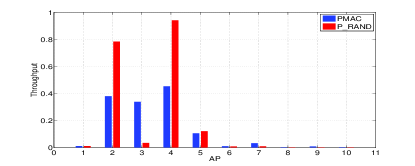
VI-C Compare with PMAC

We perform a similar comparison with PMAC. We start with a comparison of overall contention order under different SNR constraints in Fig.9 (under attempt rate $p_{c}=0.6$, same for Fig.10). With a higher base SNR, the required transmission power is potentially higher under PMAC, and thus the total contention order increases. The contention order under P_RAND on the other hand stays constant.

Figure 9: Contention order comparison

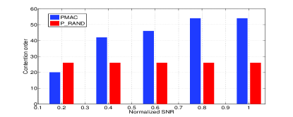
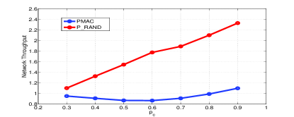
We see that in order to reduce the contention order the APs again act rather conservatively in reducing their power levels. This leads to a drop in noise resistance and the overall network throughput, as shown in Fig.10 and Fig. 11, respectively.

Figure 10: APs’ individual throughput

Figure 11: Comparison of network’s total throughput

VII Related works

There have been many classical PHY layer power-tune studies using Shannon’s capacity formula. For example, Kim et al. investigated a transmit power and carrier sensing threshold tuning problem for improving spatial reuse in [3]. Chiang et al. looked into the transmit power control problem through management of interference, energy and connectivity in [2]. In [5], Phan et al. investigate distributed power control problem on physical layer; a distributed algorithm is given and critical performance criteria, such as convergence are analyzed. In [11], Tan et al. analyze several multi-user spectrum management problems with focus on power control.

More recently, power control problems have been analyzed under game theoretical framework. Sharma et al. proposed a game theoretical approach for decentralized power allocation in [6]. In [9], a congestion game model is proposed to analyze power control problem as a form of resource allocation. Equilibrium strategies have been given under certain assumptions. In [12], a power control problem is modeled as repeated games with strategic users and intervention theory is proposed to induce target strategy from users. Imperfect monitoring repeated game model is analyzed in [13] with the assumption of a Local Spectrum Server (LSS). In [10], Wan et al. consider a power control problem w.r.t. reducing contention order on the link layer while keeping the physical layer interference under certain levels.

In terms of computation, for standard integer optimization (or combinatorial optimization) problems researchers typically seek relaxation to convert the problem into a continuous problem in the hope it can be solved by standard LP or convex algorithms; in [14, 4, 7], efficient search algorithms have been proposed to tackle finite space optimization problems.

VIII Conclusion

With the proliferation of densely-deployed WLANs, power tuning becomes a critical problem as it has major impacts on SNR as well as contention levels in these networks. Prior works mostly focused on one of these two issues in pursuit of either higher throughput or lower contention level, but not both.

In this paper, we have investigated the network throughput optimization problem by optimizing both spatial reuse (MAC) and SNR (PHY) performance at the same time. We have presented the complexity of solving the joint optimization problem and derived approximations to make it tractable. Then, by analyzing the problem structure, we have proposed efficient and near-optimal solutions. In order to demonstrate the effectiveness of our approach, we compared our results with several models optimizing on only either PHY or MAC layer. A clear advantage has been demonstrated for the cross-layer approach.

In the second part, we first show that the N.E. for the decentralized WLAN appears to be inefficient; then we show specific punishment mechanism can be designed to enforce the social near-optimal solution with our system under both perfect and imperfect monitoring environment.

References

- [1] Shoshana Anily and Awi Federgruen. Ergodicity in parametric nonstationary markov chains: An application to simulated annealing methods. Operations Research, 35(6):pp. 867–874, 1987.
- [2] Mung Chiang, Prashanth Hande, Tian Lan, and Chee Wei Tan. Power control in wireless cellular networks. Found. Trends Netw., 2(4):381–533, April 2008.
- [3] Tae-Suk Kim, Hyuk Lim, and Jennifer C. Hou. Improving spatial reuse through tuning transmit power, carrier sense threshold, and data rate in multihop wireless networks. In Proceedings of the 12th annual international conference on Mobile computing and networking, MobiCom ’06, pages 366–377, New York, NY, USA, 2006. ACM.
- [4] S. Kirkpatrick, C. D. Gelatt, and M. P. Vecchi. Optimization by simulated annealing. Science, 220:671–680, 1983.
- [5] Khoa T. Phan, Long Bao Le, Sergiy A. Vorobyov, and Tho Le-Ngoc. Centralized and distributed power allocation in multi-user wireless relay networks. In Proceedings of the 2009 IEEE international conference on Communications, ICC’09, pages 4396–4400, Piscataway, NJ, USA, 2009. IEEE Press.
- [6] Shrutivandana Sharma and Demosthenis Teneketzis. A game-theoretic approach to decentralized optimal power allocation for cellular networks. In Proceedings of the 3rd International Conference on Performance Evaluation Methodologies and Tools, ValueTools ’08, pages 1:1–1:10, ICST, Brussels, Belgium, Belgium, 2008. ICST (Institute for Computer Sciences, Social-Informatics and Telecommunications Engineering).
- [7] Yang Song, Chi Zhang, and Yuguang Fang. Throughput maximization in multi-channel wireless mesh access networks. 2012 20th IEEE International Conference on Network Protocols (ICNP), 0:11–20, 2007.
- [8] Chee Wei Tan, Daniel P. Palomar, and Mung Chiang. Solving nonconvex power control problems in wireless networks: low sir regime and distributed algorithms. In GLOBECOM, page 6, 2005.
- [9] Cem Tekin, Mingyan Liu, Richard Southwell, Jianwei Huang, and Sahand Haji Ali Ahmad. Atomic congestion games on graphs and their applications in networking. IEEE/ACM Trans. Netw., 20(5):1541–1552, 2012.
- [10] Peng-Jun Wan, Dechang Chen, Guojun Dai, Zhu Wang, and F. Frances Yao. Maximizing capacity with power control under physical interference model in duplex mode. In INFOCOM, pages 415–423, 2012.
- [11] Chee wei Tan, S. Friedland, and S.H. Low. Spectrum management in multiuser cognitive wireless networks: Optimality and algorithm. Selected Areas in Communications, IEEE Journal on, 29(2):421–430, 2011.
- [12] Yuanzhang Xiao, Jaeok Park, and Mihaela van der Schaar. Repeated games with intervention: Theory and applications in communications. CoRR, abs/1111.2456, 2011.
- [13] Yuanzhang Xiao and Mihaela van der Schaar. Dynamic spectrum sharing among repeatedly interacting selfish users with imperfect monitoring. CoRR, abs/1201.3328, 2012.
- [14] H. Peyton Young. Individual Strategy and Social Structure. Princeton University Press, 1998.