Abstract

The expansion rate of the Universe changes with time, initially slowing (decelerating) when the universe was matter dominated, because of the mutual gravitational attraction of all the matter in it, and more recently speeding up (accelerating). A number of cosmological observations now strongly support the idea that the Universe is spatially flat (provided the dark energy density is at least approximately time independent) and is currently undergoing an accelerated cosmological expansion. A majority of cosmologists consider “dark energy” to be the cause of this observed accelerated cosmological expansion.

The “standard” model of cosmology is the spatially-flat $\Lambda$CDM model. Although most predictions of the $\Lambda$CDM model are reasonably consistent with measurements, the $\Lambda$CDM model has some curious features. To overcome these difficulties, different Dark Energy models have been proposed. Two of these models, the XCDM parametrization and the slow rolling scalar field model $\phi$CDM, along with “standard” $\Lambda$CDM, with the generalization of XCDM and $\phi$CDM in non-flat spatial geometries are considered here and observational data are used to constrain their parameter sets.

In this thesis, we start with a overview of the general theory of relativity, Friedmann’s equations, and distance measures in cosmology. In the following chapters we explain how we can constrain the three above mentioned cosmological models using three data sets: measurements of the Hubble parameter $H(z)$, Supernova (SN) apparent magnitudes, and the baryonic acoustic oscillations (BAO) peak length scale, as functions of redshift $z$. We then discuss constraints on the deceleration-acceleration transition redshift $z_{\rm da}$ using unbinned and binned $H(z)$ data. Finally, we incorporate the spatial curvature in the XCDM and $\phi$CDM model and determine observational constraints on the parameters of these expanded models.

Abstract

The expansion rate of the Universe changes with time, initially slowing (decelerating) when the universe was matter dominated, because of the mutual gravitational attraction of all the matter in it, and more recently speeding up (accelerating). A number of cosmological observations now strongly support the idea that the Universe is spatially flat (provided the dark energy density is at least approximately time independent) and is currently undergoing an accelerated cosmological expansion. A majority of cosmologists consider “dark energy” to be the cause of this observed accelerated cosmological expansion.

The “standard” model of cosmology is the spatially-flat $\Lambda$CDM model. Although most predictions of the $\Lambda$CDM model are reasonably consistent with measurements, the $\Lambda$CDM model has some curious features. To overcome these difficulties, different Dark Energy models have been proposed. Two of these models, the XCDM parametrization and the slow rolling scalar field model $\phi$CDM, along with “standard” $\Lambda$CDM, with the generalization of XCDM and $\phi$CDM in non-flat spatial geometries are considered here and observational data are used to constrain their parameter sets.

In this thesis, we start with a overview of the general theory of relativity, Friedmann’s equations, and distance measures in cosmology. In the following chapters we explain how we can constrain the three above mentioned cosmological models using three data sets: measurements of the Hubble parameter $H(z)$, Supernova (SN) apparent magnitudes, and the baryonic acoustic oscillations (BAO) peak length scale, as functions of redshift $z$. We then discuss constraints on the deceleration-acceleration transition redshift $z_{\rm da}$ using unbinned and binned $H(z)$ data. Finally, we incorporate the spatial curvature in the XCDM and $\phi$CDM model and determine observational constraints on the parameters of these expanded models.

Acknowledgments

Finishing a PhD in physics is truly a marathon event, and it would have not been possible for me to finish this long and tedious journey without the help of countless people that were around me in last four years. Some of them were not with me physically during this PhD, but they are in my heart all the time. I must first express my gratitude towards my advisor Bharat Vishnu Ratra. He is an outstanding mentor and teacher. His leadership, support, guidance, attention to detail, hard work, patience and kindness have set an example I hope to match some day. Thank you for your help and guidance. I would like to thank Larry Weaver from whom I have learned a lot. He taught me more than I could read in any book on physics. He is always in his office and very welcoming. I would like to thank my roommate, my colleague and co-author of a couple of my papers, Data Mania, who helped me a lot in understanding cosmology. He is the best roommate one can have. Thanks Data. I also want to say thanks to my fellow graduate students Shawn Westmoreland and Mikhail Makouski for having very helpful discussions with me during my research. I want to thank my sister Saima Farooq and my friend Arjun Nepal and his family for being an excellent support to me during my stay here in Manhattan. Thanks to Foram Madiyar and Misty Long for being good friends to me. I want to thank all of my students whom make me think about physics problems more deeply, and their questions deepen my understanding of physics. I am extremely fortunate to have an enthusiastic and talented proofreaders in the form of Shawn Westmoreland, Max Goering, Sara Crandall and Levi Delissa. I want to say special thanks to them for spending lot of time in pointing out lots of inevitable mistakes and typos and places where my presentation didn’t sparkle quite as much as I thought it did. Their sharp eyes and hard work did much to make this thesis better. Any remaining errors or omissions are obviously the sole responsibility of mine. Special thanks to Sara Crandall co-author of one of my paper. I enjoyed working with her alot. Thanks to Daniel Nelson, my undergraduate student for letting me use his computer for some of the calculations during my work at Kansas State University. I want to give a very special thanks, though this word “thanks” is not enough for my best friend May Ebbeni, for teaching me most of physics and being one of the best friends one can ever have. You helped make 4 years of my life in graduate school more fun and interesting. Thanks alot May. Finally, and most importantly, this work would not have been possible without the endless support and encouragement from my parents. I dedicate this thesis to them. I will always remember the wonderful time that I spend here with my friends, graduate student and teachers in Physics department of Kansas State Univerity.

This work was supported in part by DOE grant DEFG03-99EP41093 and NSF grant AST-1109275.

Dedication

To my parents Farooq Ahmad Uppal and Abida Bano who trust in me in all respect more than I do myself.

Chapter 0 Introduction

Cosmology is the study of the Universe, or cosmos, regarded as a whole. Physical cosmology is the scholarly and scientific study of the origin, evolution, structure, dynamics, and ultimate fate of the Universe, as well as the natural laws that keep it in order. The study of cosmology is fueled by the curiosity of wanting to know more about the Universe in which we are living and wanting to find answers to some fundamental questions like Where do we come from? What are we? Where are we going? Does the Universe have a beginning? Will the Universe have an end? Is the Universe infinite? How did we get here? Are we special? Cosmology grapples with these questions by describing the past, explaining the present, and predicting the future of the Universe. In this chapter, we will summarize the basics and fundamentals of Einstein general theory of relativity and Friedmann’s equations undoubtedly the most important equation in cosmology. After that we will solve Friedmann’s equation in different cases.

1 Basics and Fundamentals

The structure of any theory in science is based on some fundamental axioms, often summarized generally by a genius, based on a lot of observations. These are the axioms on which the theory depends, which are sometimes incompletely experimentally tested, but, if one does not believe in these axioms then one does not believe in the theory. The theory, which is generally a mathematical formula, will make some predictions that one has to develop experimental set-up to check. If the theory make predictions that are consistent with the experimental results within the uncertainty of the experimental error, this means that the theory can be trusted, until we have some experiment which gives a contradictory result. In this case it is said that the theory needs modifications. After finding a number of experimental results consistent with the predictions of the theory, the theory is accepted by the scientific community and one can make deductions from it. On the other hand, if the theory gives results that disagree with experiments, then the theory is wrong, independent of who developed the theory, how beautiful the theory is, and how smart the person who developed it is.

Standard, cosmology is based on a fundamental axiom, the cosmological principle. This principle states that Universe is homogeneous and isotropic in space on a sufficiently large scale (roughly $100$ Mpc or more). This simply means that there is no special location for any observer, in any part of cosmos, and the large-scale picture of the Universe will look the same from any point is space.

Going back to history, Newtonian mechanics is an approximation which works quite well for most of our “earthly” needs, at least when the velocity $v\ll c$ where $c$ is the speed of light. A more general theory was developed by Albert Einstein. The basic differences and analogies between Newtonian and Einsteinian physics are presented in Table (1).

Newtonian Mechanics.	Einsteinian Mechanics.
Absolute time and absolute space.	Dynamical spacetime, one entity.
Galilean invariance of space (simultaneity).	Lorentz invariance of spacetime (time dilation, length contraction, no simultaneity).
Existence of preferred inertial frames (at rest or moving with constant velocity w.r.t. absolute space).	No preferred frames (physics is the same everywhere).
Infinite speed of light $c$ (instantaneous action at a distance).	Finite and fixed speed of light $c$ (nothing physical can propagate faster than c).
There is no upper limit on the speed with which mass can travel.	There is a upper limit of speed with which mass can travel, $c$.
Gravity is a force.	Gravity is a distortion of the fabric of spacetime.
Newton’s Second Law:	Geodesic equation:
$\frac{d^{2}x^{i}}{dt^{2}}=-\delta^{ij}\frac{\partial\Phi}{\partial x^{j}}$.	$\frac{d^{2}x^{\nu}}{d\lambda^{2}}=-\Gamma^{\nu}_{\gamma\delta}\frac{dx^{\gamma}}{d\lambda}\frac{dx^{\delta}}{d\lambda}$.
Poisson equation:	Einstein’s field equation:
${\nabla}^{2}\Phi(x)=4\pi G\rho_{m}$	$G_{\mu\nu}=8\pi GT_{\mu\nu}$
Mass produces a field $\Phi$ causing a force on the other mass $m$ given by:	Spacetime is curved and mass particles move along curved geodesics defined by metric:
$\vec{F}=-\vec{\nabla}\Phi$.	$ds^{2}=g_{\mu\nu}(x)dx^{\mu}dx^{\nu}$.
Absolute space acts on matter but is not acted upon (Newton’s interpretation of the bucket experimenta ).b	Spacetime acts on matter and is acted upon by matter (Einstein’s field equation).

Differences and analogies between Newtonian and Einsteinian mechanics.

• Interested readers can read more about it in the Principia ¹¹⁴ or on Wikipedia.

• Special thanks to Shawn Westmoreland.

Newtonian mechanics quickly runs into phenomenon that it cannot explain:

• Why do all observers measure the same speed of light $c$ (in a vacuum), as demonstrated by the Michelson-Morley experiment?

• Why don’t Maxwell’s equations respect Galilean invariance?

• Why do all bodies experience the same gravitational acceleration regardless of their mass? Why are the inertial and gravitational mass the same (as measured experimentally)?

• Why does the perihelion of the orbit of Mercury not behave as required by Newton’s equations?

To answer some of these questions, Einstein proposed his theory of Special Relativity in 1905, in which he introduced some revolutionary concepts:

• “Abolished” absolute time — introduced 4-dimensional spacetime as an inseparable entity.

• However, the 4-dimensional spacetime considered in special relativity is still flat Minkowski spacetime.

• Finite and fixed speed of light $c$, independent of the observer.

• Established the equivalence between energy and mass.

• Prohibition on any particle with non-zero rest mass to move with speed $v\geq c$.

Einstein’s theory of General Relativity, which he proposed in 1915, continued the revolution by adding the following ideas to the intellectual data base of humanity:

• Equivalence principle: Established the equivalence between inertial and gravitational mass.

• Cosmological principle: Our position is “as mundane as it can be” (on large spatial scales, the Universe is homogeneous and isotropic).

• Relativity: The laws of physics are the same everywhere.

• New definition of gravity: Gravity is not a force but the distortion of the structure of spacetime as caused by the presence of matter and energy. The paths followed by matter and energy in spacetime are governed by the structure of spacetime. This great feedback loop is described by Einstein’s field equation. In the beautiful words of John Wheeler “Mass-energy tells space-time how to curve, Curved space-time tells mass-energy how to move.” So the 4-dimensional spacetime considered in general relativity is no longer flat (no longer Minkowskian).

After establishing general relativity as the way to describe the Universe and learning its mathematical formalism, we will finally embark on a journey of expressing, mathematically, the world around us on larger scales, and physically interpreting the implications of this and relating this to the observations. Many of the phenomena for which we now have overwhelming evidence, for — the big bang, the expanding and accelerated Universe, the cosmic microwave background (CMB) radiation, black holes, among others — were first predicted from Einstein’s field equation. Therefore, it is the mathematics that hold the keys to unlocking the mysteries of the Universe. So let us begin by reviewing the required mathematical ideas.

2 Mathematical Background

1 Notation

In this section we will develop some basic mathematical notations needed for general relativity.

4-vectors:   $(t,x,y,z)\equiv(x^{0},x^{1},x^{2},x^{3})=x^{\mu}$.

Conventions for indices:

• Roman letters $(i,j,k,l,m,n)$ run from 1 to 3;

• Greek letters $(\alpha,~{}\beta,~{}\gamma,~{}\delta,~{}\mu,~{}\nu,~{}\eta,~{}\xi)$ run from 0 to 3.

Einstein summation: (summation over repeated indices): $\mu^{\prime\alpha}=\sum\limits_{\beta=0}^{3}{\frac{\partial x^{\prime\alpha}}{\partial x^{\beta}}\mu^{\beta}\equiv\frac{\partial x^{\prime\alpha}}{\partial x^{\beta}}\mu^{\beta}}$. Under change of coordinates $x^{\beta}\rightarrow x^{\prime\beta}.$

Contravariant vector: (index is a superscript) transforms as $A^{\prime\alpha}=\frac{\partial x^{\prime\alpha}}{\partial x^{\beta}}A^{\beta}$

Covariant vector: (index is a subscript) transforms as $A^{\prime}_{\alpha}=\frac{\partial x^{\beta}}{\partial x^{\prime\alpha}}A_{\beta}$

Tensors: These are objects with multiple indices.

$$\rm First~{}~{}rank~{}~{}tensor~{}~{}(one~{}~{}index):\left\{\begin{array}[]{lr}\vspace{6pt}\rm{contravariant}:\textit{A}^{\prime\alpha}=\frac{\partial x^{\prime\alpha}}{\partial x^{\beta}}\textit{A}^{\beta}.\\ \vspace{6pt}\rm{covariant}:\textit{A}^{\prime}_{\alpha}=\frac{\partial x^{\beta}}{\partial x^{\prime\alpha}}\textit{A}_{\beta}.\\ \end{array}\right.$$ (1)

$$\rm Second~{}~{}rank~{}~{}Tensor~{}~{}(two~{}~{}indices):\left\{\begin{array}[]{lr}\vspace{6pt}\par\rm{contravariant}:\textit{A}^{\prime\alpha\beta}=\frac{\partial x^{\prime\alpha}}{\partial x^{\xi}}\frac{\partial x^{\prime\beta}}{\partial x^{\nu}}\textit{A}^{\xi\nu}.\\ \vspace{6pt}\par\rm{covariant}:\textit{A}^{\prime}_{\alpha\beta}=\frac{\partial x^{\alpha}}{\partial x^{\prime\xi}}\frac{\partial x^{\beta}}{\partial x^{\prime\nu}}\textit{A}_{\xi\nu}.\\ \vspace{6pt}\par\rm{mixed}:\textit{A}^{\prime\alpha}_{\beta}=\frac{\partial x^{\prime\alpha}}{\partial x^{\xi}}\frac{\partial x^{\nu}}{\partial x^{\prime\beta}}\textit{A}_{\nu}^{\xi}.\\ \end{array}\right.$$ (2)

$$\rm N^{th}~{}~{}rank~{}~{}Tensor~{}~{}(\textit{N}~{}~{}indices):\left\{\begin{array}[]{lr}\vspace{6pt}\par\rm{mixed}:\textit{A}^{\prime\alpha_{1}...\alpha_{s}}_{\alpha_{s+1}...\alpha_{N}}=\frac{\partial x^{\prime\alpha_{1}}}{\partial x^{\beta_{1}}}...\frac{\partial x^{\prime\alpha_{s}}}{\partial x^{\beta_{s}}}\frac{\partial x^{\alpha_{s+1}}}{\partial x^{\prime\beta_{s+1}}}...\frac{\partial x^{\alpha_{N}}}{\partial x^{\prime\beta_{N}}}\textit{A}_{\beta_{s+1}...\beta_{N}}^{\beta_{1}...\beta_{s}}.\\ \end{array}\right.$$ (3)

Tensor Operations:

• Addition: $A^{\alpha\beta}_{\mu\nu}+B^{\alpha\beta}_{\mu\nu}=C^{\alpha\beta}_{\mu\nu}$

• Subtraction: $A^{\alpha\beta}_{\mu\nu}-B^{\alpha\beta}_{\mu\nu}=D^{\alpha\beta}_{\mu\nu}$

• Tensor Product: $A^{\alpha\beta}_{\mu\nu}~{}B^{\gamma\delta}_{\eta\xi}=F^{\alpha\beta\gamma\delta}_{\mu\nu\eta\xi}$

• Contraction: $A^{\alpha\psi}_{\psi\gamma}=H^{\alpha}_{\gamma}$        (summed over $\psi$)

• Inner Product: $A^{\alpha\beta}_{\mu\nu}~{}B^{\nu\gamma}_{\delta\eta}=P^{\alpha\beta\nu\gamma}_{\mu\nu\delta\eta}=K^{\alpha\beta\gamma}_{\mu\delta\eta}$

Why Tensors are Important:

When the equations of motion are written in tensor form, they are invariant under some appropriately-defined transformations. For example:

• Newtonian Mechanics: 3 - vectors $(x,y,z)=(x^{1},x^{2},x^{3})$ are invariant under Galilean transformations.

• Special Relativity: 4 - vectors $(t,x,y,z)=(x^{0},x^{1},x^{2},x^{3})$ are invariant under Lorentz transformations.

• General Relativity: 4 - vectors $(t,x,y,z)=(x^{0},x^{1},x^{2},x^{3})$ are invariant under general coordinate transformations.

Scalar: They are invariant, which means they are the same in all coordinate systems.

2 Metric Tensor

Flat Euclidean space

Our everyday experience has taught us to think in terms of a flat space metric (Euclidean), where parallel lines never cross and the sum of the interior angles of a triangle is $180^{0}$. In this case, the invariant line element of space in Cartesian coordinates $(x,y,z)=(x^{1},x^{2},x^{3})$ is:

$$ds^{2}=(dx^{1})^{2}+(dx^{2})^{2}+(dx^{3})^{2},$$ (4)

and space is flat. An equivalent way of writing the above metric is:

$$ds^{2}=\delta_{ij}dx^{i}dx^{j},$$ (5)

where $\delta_{\alpha\beta}$ is the Kronecker delta function defined as:

$$\delta_{\alpha\beta}=\left\{\begin{array}[]{cc}1&\mathrm{for}\ \alpha=\beta,\\ 0&\mathrm{for}\ \alpha\neq\beta.\\ \end{array}\right.$$ (6)

Therefore, the Euclidean space metric tensor for Cartesian coordinates is:

$$\delta_{ij}=\left({\begin{array}[]{ccc}1&0&0\\ 0&1&0\\ 0&0&1\\ \end{array}}\right).$$ (7)

An invariant line element in an arbitrary coordinate system in flat space, can be written in terms of Cartesian coordinates (via change of variables):

$$ds^{2}=\delta_{ij}dx^{i}dx^{j}=\delta_{ij}\left(\frac{\partial x^{i}}{\partial x^{\prime k}}dx^{\prime k}\right)\left(\frac{\partial x^{j}}{\partial x^{\prime l}}dx^{\prime l}\right)=\delta_{ij}\frac{\partial x^{i}}{\partial x^{\prime k}}\frac{\partial x^{j}}{\partial x^{\prime l}}dx^{\prime k}dx^{\prime l}\equiv p_{kl}dx^{\prime k}dx^{\prime l}.$$ (8)

where $p_{kl}$ is the metric of the new coordinate system.

Since the line element is invariant under the interchange of $dx^{\prime}$ and $dx$, we may, without loss of generality, take the metric tensor to be symmetric in general relativity. Furthermore, isotropy and homogeneity (as in the flat Euclidean space) implies that the metric tensor in such a space will necessarily be diagonal.

Consider an example of spherical coordinates $(r,\theta,\phi)$, Fig. (1), where we are at the center of the spherical coordinate system. As we look out into the “cosmos,” the flat space part of the metric (line element) is given by the following line element:⁷³

$$ds^{2}=dr^{2}+r^{2}\left(d\theta^{2}+\mathrm{sin^{2}}\theta d\phi^{2}\right),$$ (9)

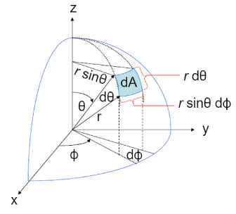
Figure 1: Spherical coordinate system. Figure shows $r=$ constant surface, hence, $dr=0$ on the surface.

where $\theta$ is now measured from the north pole and is $\pi$ at the south pole. It is useful to abbreviate the term between parenthesis as:

$$d\Omega^{2}=d\theta^{2}+\mathrm{sin^{2}}\theta d\phi^{2},$$ (10)

because it is a measure of angle on the sky of the observer. Since the Universe is isotropic, the angle between two galaxies as we see it is, in fact, the true angle from our vantage point. The expansion of the Universe (which we will discuss later) does not change this angle [we will explain this in Sec. (4)]. Therefore we need only $d\Omega$. So, for flat space, the line element is:

$$ds^{2}=dr^{2}+r^{2}d\Omega^{2}.$$ (11)

Flat Minkowski Spacetime

We can now generalize the interval to 4-dimensional flat spacetime $(x^{0},x^{1},x^{2},x^{3})$:

$$ds^{2}=-(dx^{0})^{2}+(dx^{1})^{2}+(dx^{2})^{2}+(dx^{3})^{2},$$ (12)

which can be written in compact notation as:

$$ds^{2}=\eta_{\alpha\beta}dx^{\alpha}dx^{\beta},$$ (13)

where $\eta_{\alpha\beta}$ is the Minkowski (flat) spacetime metric tensor:

$$\eta_{\alpha\beta}=\left({\begin{array}[]{cccc}-1&0&0&0\\ 0&1&0&0\\ 0&0&1&0\\ 0&0&0&1\\ \end{array}}\right).$$ (14)

Again, isotropy and homogeneity of spacetime leads to a diagonal metric tensor.

Curved Three-Dimensional Space

For a general (possibly curved) covariant spacetime metric tensor $g_{\alpha\beta}$, the invariant line element is given by

$$ds^{2}=g_{\alpha\beta}dx^{\alpha}dx^{\beta}.$$ (15)

The contravariant spacetime metric tensor $g^{\alpha\beta}$ is the inverse of the covariant tensor $g_{\alpha\beta}$:

$$g^{\alpha\beta}g_{\beta\gamma}=\delta^{\alpha}_{\gamma}.$$ (16)

This implies that whenever the metric tensor is diagonal:

$$g^{\alpha\beta}=(g_{\alpha\beta})^{-1}.$$ (17)

One can take inner products of tensors with the metric tensor, thus lowering or raising indices:

$$A_{\alpha\beta}=g_{\alpha\mu}A^{\mu}_{\beta},\hskip 19.91692ptA^{\alpha\beta}=g^{\alpha\mu}A_{\mu}^{\beta}.$$ (18)

For the spatial part of $g_{\alpha\beta}$, as proven by Robertson and Walker, the only alternative line elements, beside Eq. (11), that obey both isotropy and homogeneity is:

$$ds^{2}=dr^{2}+S_{k}(r)^{2}d\Omega^{2},$$ (19)

where the function $S_{k}(r)$ is a function of space curvature given by:

$$S_{k}(r)=\left\{\begin{array}[]{cc}\frac{1}{\sqrt{k}}\ \mathrm{sin}\big{(}\sqrt{k}\ r\big{)}&\ \ \ \ \mathrm{for}\ k>0\\ r&\ \ \ \ \mathrm{for}\ k=0\\ \frac{1}{\sqrt{-k}}\ \mathrm{sinh}\big{(}\sqrt{-k}\ r\big{)}&\ \ \ \ \mathrm{for}\ k<0\\ \end{array},\right.$$ (20)

where the central $k=0$ case is given in Eq. (11). This means that the circumference of a sphere around us with radius $r$, for $k\neq 0$, is no longer equal to $C=2\pi r$, but is smaller for $k>0$ and larger for $k<0$. Also, the surface area of that sphere is no longer $S=4\pi r^{2}$, but is smaller for $k>0$ and larger for $k<0$. For small $r$ (to be precise, for $r\ll|{k}|^{−1/2}$ ) the deviation from $C=2\pi r$ and $S=4\pi r^{2}$ is small, but as $r$ approaches $|{k}|^{−1/2}$ the deviation can become very large. This can be checked by writing the Taylor’s series expansion of Eq. (20). This is very similar to the 2-dimensional example of the Earth’s surface.

If we stand on the North Pole, and use $r$ as the distance from us along the sphere (i.e. the longitudinal distance) from the north pole and $d\phi$ as the 2-dimensional version of $d\Omega$, then the circumference of a circle at $r=10000$ km (i.e. a circle that is the equator in this case) is “just” 40000 km instead of $2\pi\times 10000=62831$ km, i.e. a factor of 0.63 smaller than it would be on a flat surface.

The constant $k$ is the curvature constant. We can also define a “radius of curvature”, as:

$$R_{\mathrm{curvature}}=|k|^{-1/2},$$ (21)

which, for our 2-dimensional example of the Earth’s surface, is the radius of the Earth. In our 3-dimensional Universe it is the radius of a 3-dimensional “surface” of a 4-dimensional “sphere” in 4-dimensional space.

Note that the expression given in Eq. (19) is not the only possible way of writing the metric in curved space. For instance, if we switch to a very commonly used parametrization in which we change the radial coordinate from $r$ to $x\equiv S_{k}(r)$, then from Eq. (20):

$$r=\left\{\begin{array}[]{cc}\vspace{0.2cm}\frac{1}{\sqrt{k}}\ \mathrm{sin^{-1}}\left(\sqrt{k}\ x\right)&\ \ \ \ \mathrm{for}\ k>0\\ \vspace{0.2cm}x&\ \ \ \ \mathrm{for}\ k=0\\ \vspace{0.2cm}\frac{1}{\sqrt{-k}}\ \mathrm{sinh^{-1}}\Big{(}\sqrt{-k}\ x\Big{)}&\ \ \ \ \mathrm{for}\ k<0\\ \end{array},\right.$$ (22)

which implies that:

$$dr=\left\{\begin{array}[]{cc}\vspace{0.2cm}\frac{1}{\sqrt{k}}\left(\frac{\sqrt{k}}{\sqrt{1-\left(\sqrt{k}x\right)^{2}}}dx\right)&\ \ \ \ \mathrm{for}\ k>0\\ \vspace{0.2cm}dx&\ \ \ \ \mathrm{for}\ k=0\\ \vspace{0.2cm}\frac{1}{\sqrt{-k}}\left(\frac{\sqrt{-k}}{\sqrt{1+\left(\sqrt{-k}x\right)^{2}}}dx\right)&\ \ \ \ \mathrm{for}\ k<0\\ \end{array}.\right.$$ (23)

By squaring both sides of Eq. (23) we get:

$$dr^{2}=\left\{\begin{array}[]{cc}\vspace{0.2cm}\frac{1}{1-kx^{2}}dx^{2}&\ \ \ \ \mathrm{for}\ k>0\\ \vspace{0.2cm}dx^{2}&\ \ \ \ \mathrm{for}\ k=0\\ \vspace{0.2cm}\frac{1}{1-kx^{2}}dx^{2}&\ \ \ \ \mathrm{for}\ k<0\\ \end{array}.\right.$$ (24)

Then, the metric for homogeneous, isotropic, 3-dimensional space can be written as

$$ds^{2}=\frac{dx^{2}}{1-kx^{2}}+x^{2}d\Omega^{2},$$ (25)

which we can rewrite, by changing the name of the variable from $x$ to $r$, as

$$ds^{2} = \frac{dr^{2}}{1-kr^{2}}+r^{2}d\Omega^{2},$$ (26)

$$\Rightarrow ds^{2} = \frac{dr^{2}}{1-kr^{2}}+r^{2}\left(d\theta^{2}+\mathrm{sin^{2}}\theta d\phi^{2}\right).$$ (27)

Note that this metric is different only in the way we choose our coordinate $r$; it is not different in any physical way from Eq. (19).

Expanding flat spacetime.

The metric tensor for a flat, homogeneous, and isotropic spacetime, which is expanding or contracting spatially with scale factor $a(t)$, is obtained from the Minkowski metric by scaling the spatial coordinates by $a^{2}(t)$:

$$g_{\alpha\beta}=\left({\begin{array}[]{cccc}-1&0&0&0\\ 0&a^{2}(t)&0&0\\ 0&0&a^{2}(t)&0\\ 0&0&0&a^{2}(t)\\ \end{array}}\right).$$ (28)

Then the metric takes the form:

$$ds^{2}=-dt^{2}+a^{2}(t)\left[dr^{2}+r^{2}d\Omega^{2}\right].$$ (29)

In Cartesian coordinates:

$$ds^{2}=-dt^{2}+a^{2}(t)d{x}^{2},$$ (30)

where $dx$ is known as the coordinate or comoving infinitesimal distance while $adx$ is the physical or proper infinitesimal distance.

Expanding curved spacetime (Friedmann-Lemaître-Robertson-Walker metric tensor).

In cosmology, a common zeroth order approximation is to slice spacetime into spacelike slices which are exactly homogeneous and isotropic. This means that there exists a coordinate system in which the constant $t$ hypersurfaces are homogeneous and isotropic. The proper time $t$, which labels the hypersurfaces, is called the cosmic time.

There is evidence that the Universe is indeed statistically homogeneous (all places look the same) and isotropic (all directions look the same) on scales larger than few 100 Mpc, as we noted at the beginning of the chapter. This does not prove that the Universe is well described by a model which is exactly homogeneous and isotropic, but it does motivate us to use it as a first approximation. We shall see that this approximation, is in fact, quite good, and at early times it is excellent, as the Universe was then more homogeneous and isotropic.

Since the spacetime is spatially homogeneous and isotropic, its curvature is the same at all points in space, but can vary in time. It can be shown that the spacetime metric of curved expanding space can be written (by a suitable choice of the coordinates) in the form:^{98, 182, 89, 115}

$$ds^{2}=-dt^{2}+a^{2}(t)\left[\frac{dr^{2}}{1-kr^{2}}+r^{2}d\theta^{2}+r^{2}\mathrm{sin^{2}}\theta d\phi^{2}\right].$$ (31)

An alternative form, in Cartesian as opposed to spherical coordinates, is

$$ds^{2}=-dt^{2}+a^{2}(t)\frac{1}{(1+\frac{k}{4}r^{2})^{2}}\delta_{ij}dx^{i}dx^{j}.$$ (32)

In either form, this is called the Robertson-Walker (RW) metric, sometimes the Friedmann-Robertson-Walker (FRW) metric or the Friedmann-Lemaître-Robertson-Walker (FLRW) metric. It was first derived by Friedmann in 1922 and then more generally by Robertson in late 1920s and early 1930’s and Walker in 1935. Note that both form of the metric has the same amount of symmetry as the spacetime itself: the metrics are isotropic, and homogeneous. The full symmetry of the spacetime is usually not apparent in the metric itself, even though all physical quantities calculated from the metric display the symmetry. The time coordinate $t$ is the cosmic time. Here $k$ is a constant, related to curvature of space (not spacetime) and $a(t)$ is a function of time which governs how the Universe expands (or contracts). In Eq. (31), the coordinates $r$, $\theta$, and $\phi$ are known as comoving coordinates. A freely moving particle is at rest in these coordinates. Equation (31) is a purely kinematic statement. In this problem, the dynamics are associated with the scale factor $a(t)$. The Einstein equations allow us to determine the scale factor $a(t)$ provided the matter content of the Universe is specified.

3 Covariant Derivative

Consider a vector $\vec{A}$ given in terms of its components along the basis vectors $\hat{e}_{\alpha}$ as:

$$\vec{A}=A^{\alpha}\hat{e}_{\alpha}.$$ (33)

Differentiating the vector $\vec{A}$ using the standard Leibniz rule for the differentiation of the product of functions $(fg)^{\prime}=f^{\prime}g+fg^{\prime}$, we get:

$$\frac{\partial\vec{A}}{\partial x^{\alpha}}=\frac{\partial}{\partial x^{\alpha}}\Big{(}A^{\beta}\hat{e}_{\beta}\Big{)}=\frac{\partial A^{\beta}}{\partial x^{\alpha}}\hat{e}_{\beta}+A^{\beta}\frac{\partial\hat{e}_{\beta}}{\partial x^{\alpha}}.$$ (34)

In flat Cartesian coordinates the basis vectors are constant, so the last term in the Eq. (34) vanishes. However, this is not the case in general curved spaces. In general, the derivative in the last term will not vanish, and it will itself be given in terms of the original basis vectors:

$$\frac{\partial\hat{e}_{\beta}}{\partial x^{\alpha}}\equiv\Gamma^{\nu}_{\alpha\beta}\hat{e}_{\nu},$$ (35)

where $\Gamma^{\nu}_{\alpha\beta}$ is called Christoffel symbol. It is given in terms of the metric tensor $g_{\mu\nu}$ as (see MWT ¹¹¹):

$$\Gamma^{\nu}_{\alpha\beta}\equiv\frac{1}{2}g^{\nu\gamma}\Big{(}g_{\alpha\gamma,\beta}+g_{\gamma\beta,\alpha}-g_{\alpha\beta,\gamma}\Big{)}.$$ (36)

Here it is important to note that Christoffel symbols are not tensors.

Taking the curvature of the ambient manifold into account when taking derivatives of a scalar field $\phi$, a vector $A^{\alpha}$, or a co-vector $A_{\alpha}$ will yield covariant derivatives:

$$\partial_{;\mu}\phi\equiv\partial_{,\mu}\phi,\hskip 25.60747ptA_{\alpha;\beta}\equiv A_{\alpha,\beta}-\Gamma^{\nu}_{\alpha\beta}A_{\nu},\hskip 25.60747ptA^{\alpha}_{;\beta}\equiv A^{\alpha}_{,\beta}+\Gamma^{\nu}_{\alpha\beta}A^{\nu},$$ (37)

where we have used the short hand notation $\partial_{,\mu}\phi\equiv\frac{\partial\phi}{\partial x^{\mu}}$, $A_{\alpha,\beta}\equiv\frac{\partial A_{\alpha}}{\partial x^{\beta}}$ and $A^{\alpha}_{,\beta}\equiv\frac{\partial A^{\alpha}}{\partial x^{\beta}}$. Other covariant derivatives of second rank contravariant and covariant tensor are defined as

$$\nabla_{\rho}A^{\mu\nu}\equiv A^{\mu\nu}_{;\rho}\equiv A^{\mu\nu}_{,\rho}+\Gamma^{\mu}_{\rho\alpha}A^{\alpha\nu}+\Gamma^{\nu}_{\rho\beta}A^{\mu\beta},$$ (38)

$$\nabla_{\rho}A_{\mu\nu}\equiv A_{\mu\nu;\rho}\equiv A_{\mu\nu,\rho}-\Gamma^{\alpha}_{\rho\mu}A_{\alpha\nu}-\Gamma^{\beta}_{\rho\nu}A_{\mu\beta},$$ (39)

respectively. The covariant derivative of mixed tensor is defined as

$$\nabla_{\rho}A^{\mu}_{\nu}\equiv A^{\mu}_{\nu;\rho}\equiv A^{\mu}_{\nu,\rho}+\Gamma^{\mu}_{\rho\alpha}A^{\alpha}_{\nu}-\Gamma^{\beta}_{\rho\nu}A^{\mu}_{\beta},$$ (40)

where $A^{\mu\nu}_{,\rho}=\frac{\partial A^{\mu\nu}}{\partial x^{\rho}}$, $A_{\mu\nu,\rho}=\frac{\partial A_{\mu\nu}}{\partial x^{\rho}}$, and $A^{\mu}_{\nu,\rho}=\frac{\partial A^{\mu}_{\nu}}{\partial x^{\rho}}$.

For vector $A^{\alpha}$, and co-vector $A_{\alpha}$, defined along a curve $x^{\beta}=x^{\beta}(s)$, the covariant derivative along this curve are

$$\frac{DA^{\alpha}}{Ds}\equiv\frac{dA^{\alpha}}{ds}+\Gamma^{\alpha}_{\beta\gamma}\frac{dx^{\gamma}}{ds}A^{\beta},\hskip 19.91692pt\frac{DA_{\alpha}}{Ds}\equiv\frac{dA_{\alpha}}{ds}-\Gamma^{\beta}_{\alpha\gamma}\frac{dx^{\gamma}}{ds}A_{\beta},$$ (41)

The covariant derivative in a curved spacetime is the analog to the ordinary derivative in Cartesian coordinates in flat spacetime.

Principle of General Covariance

This principle states that all tensor equations valid in Special Relativity will also be valid in General Relativity if:

• The Minkowski metric $\eta_{\alpha\beta}$ is replaced by a general curved metric $g_{\alpha\beta}$.

  $$ds^{2}=\eta_{\alpha\beta}dx^{\alpha}dx^{\beta} \Rightarrow ds^{2}=g_{\alpha\beta}dx^{\alpha}dx^{\beta}$$ (42)

  $$\eta_{\alpha\beta}u^{\alpha}u^{\beta}=-1 \Rightarrow g_{\alpha\beta}u^{\alpha}u^{\beta}=-1,$$ (43)

• All the partial derivatives are replaced by covariant derivatives; in simple language the commas in the equations will be replaced by semicolon (, $\rightarrow$ ;). E.g.,

  $$T^{\alpha\beta}_{,\beta}=0 \Rightarrow T^{\alpha\beta}_{;\beta}=0.$$ (44)

4 Geodesic Equation

The fundamental axiom on which Newtonian mechanics is based is Newton’s second Law, which states that when a net force $\vec{F}$ acts on a body of mass $m$ it produces acceleration $\vec{a}$ in the direction of the net force such that

$$m\frac{d^{2}\vec{x}}{dt^{2}}=\vec{F}=-\vec{\nabla}\Phi\hskip 8.53581pt\Rightarrow\hskip 8.53581pt\frac{d^{2}\vec{x}}{dt^{2}}=-\frac{1}{m}\vec{\nabla}\Phi,$$ (45)

where $\Phi$ is the scalar potential field, $d/dt$ is the time derivative and $\vec{\nabla}\Phi$ is the gradient of the scalar potential. In the absence of forces acting on a body, Newton’s second Law reduces to Newton’s first Law (which means the first Law is the special case of second Law),

$$\frac{d^{2}\vec{x}}{dt^{2}}=-\frac{1}{m}\vec{\nabla}\Phi=0.$$ (46)

In flat Euclidean space and flat Minkowski spacetime, this also leads to straight lines.

It is a fundamental assumption of general relativity that, in curved spacetime, free particles (i.e., particles feeling no non-gravitational effects) follow paths that extremize their proper interval $ds$. Such paths are called geodesics. Therefore, generalizing Newton’s Laws of motion of a particle in the absence of forces, Eq. (46), to a general curved spacetime metric, leads to the geodesic equation.

Derivation of geodesic equation.

We derive the geodesic equation using the variational principle (Lagrange’s equation).

Suppose the points $x^{i}$ lie on a curve parametrized by the parameter $\psi$, i.e.,

$$x^{\alpha}\equiv x^{\alpha}(\psi),\hskip 28.45274ptdx^{\alpha}=\frac{dx^{\alpha}}{d\psi}d\psi,$$ (47)

and the distance between two points A and B is denoted by $S_{AB}$ and is given by

$$S_{AB}=\int\limits_{A}^{B}ds=\int\limits_{A}^{B}\frac{ds}{d\psi}d\psi={{\int}}\limits_{A}^{B}\sqrt{g_{\alpha\beta}\frac{dx^{\alpha}}{d\psi}\frac{dx^{\beta}}{d\psi}}d\psi.$$ (48)

The shortest path between the points A and B is called the geodesic, and it is found by extremizing (minimizing) the path $S_{AB}$. This is done using the standard tools of variational calculus and leads to the Lagrange equations; we review this technique next.

Consider a functional $G(x)$ of the form:

$$G(x)\equiv{{\int}}\limits^{B}_{A}L\left(\lambda,x,\frac{dx}{d\lambda}\right)d\lambda.$$ (49)

Note that here our curve is parametrized by $\lambda$. Let $x=\rm X(\lambda)$ be the curve extremizing $G(x)$ (this is what we are looking for). Then a nearby curve passing through A and B can be parametrized as $x=\rm X(\lambda)+\varepsilon\eta(\lambda)$, such that $\eta(A)=\eta(B)=0$. To extremize Eq. (49), we have to require $\frac{dG}{d\varepsilon}\Big{|}_{\varepsilon=0}=0$. This means

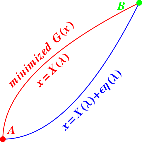
Figure 2: Variational Principle.

$$\frac{dG}{d\varepsilon}\bigg{|}_{\varepsilon=0} = \int\limits^{A}_{B}\left[\ \ \frac{\partial L}{\partial x}\frac{dx}{d\varepsilon}+\frac{\partial L}{\partial\dot{x}}\frac{d\dot{x}}{d\varepsilon}+\cancelto{0}{\frac{\partial L}{\partial\lambda}\frac{d\lambda}{d\varepsilon}}\ \ \ \ \right]d\lambda=0,\hskip 14.22636pt\left(\because\ \frac{d\lambda}{d\varepsilon}=0\right)$$ (50)

$$= \int\limits^{B}_{A}\left(\frac{\partial L}{\partial x}\eta+\frac{\partial L}{\partial\dot{x}}\dot{\eta}\right)d\lambda,\hskip 96.73936pt\left(\text{where }\dot{x}\equiv\frac{dx}{d\lambda},\ \dot{\eta}\equiv\frac{d\eta}{d\lambda}\right)$$

$$= \int\limits^{B}_{A}\frac{\partial L}{\partial x}\eta~{}d\lambda+\int\limits^{B}_{A}\frac{\partial L}{\partial\dot{x}}\dot{\eta}~{}d\lambda,$$

$$= \int\limits^{B}_{A}\frac{\partial L}{\partial x}\eta~{}d\lambda+\frac{\partial L}{\partial\dot{x}}\eta\bigg{|}_{A}^{B}-\int\limits_{A}^{B}\eta\frac{d}{d\lambda}\frac{\partial L}{\partial\dot{x}}~{}d\lambda,\hskip 17.07164pt\left(\text{here we integrated by parts}\right)$$

$$= \int\limits^{B}_{A}\frac{\partial L}{\partial x}\eta~{}d\lambda+\frac{\partial L}{\partial\dot{x}}\Bigg{|}^{B}_{A}\left[\eta(B)-\eta(A)\right]-\int\limits_{A}^{B}\eta\frac{d}{d\lambda}\frac{\partial L}{\partial\dot{x}}~{}d\lambda,$$

$$= \int\limits_{A}^{B}\eta\left[\frac{\partial L}{\partial x}-\frac{d}{d\lambda}\frac{\partial L}{\partial\dot{x}}\right]d\lambda=0.\hskip 28.45274pt\left(\text{remember}\ \eta(A)=\eta(B)=0\right).$$

But the function $\eta$ is arbitrary, so in order to have $\frac{dG}{d\varepsilon}\big{|}_{\varepsilon=0}=0$, the square brackets in the integrand must vanish, and so we arrive at Lagrange’s equation

$$\frac{\partial L}{\partial x}-\frac{d}{d\lambda}\frac{\partial L}{\partial\dot{x}}=0.$$ (51)

This can be extended to any number of phase-space coordinates as follows

$$\frac{\partial L}{\partial x^{\alpha}}-\frac{d}{d\lambda}\frac{\partial L}{\partial\dot{x}^{\alpha}}=0.$$ (52)

Euler-Lagrange equation in Scaler field theory¹⁰⁶

In the case of field theory in curved spacetime, the action $S(\Omega)$ for a scaler filed $\phi$ in an arbitrary region $\Omega$ of four-dimensional spacetime is given by:

$$S(\Omega)=\int\limits_{\Omega}\sqrt{-g}\ \mathcal{L}(\phi,\partial_{\alpha}\phi)\mathrm{d^{4}}x,$$ (53)

where the Lagrangian density $\mathcal{L}(\phi,\partial_{\alpha}\phi)$ depends on the scalar field, and the first derivatives of the scalar field with respect to the coordinates only. This is not the most general case possible, but it covers all the theories in this work. Here $g$ is the determinant of the metric $g_{\alpha\beta}$ and $\mathrm{d^{4}}x$ stands for the four-dimensional volume element $\mathrm{d}x^{0}\mathrm{d^{3}}\bf{x}$.

Now we postulate that the equations of motion (i.e., the field equations), are obtained from the variational principle.¹⁰⁶ For any region $\Omega$, we consider variations of the fields

$$\phi(x)\rightarrow\phi(x)+\delta\phi(x),$$ (54)

which vanish on the surface $\Gamma(\Omega)$ bounding the region $\Omega$:

$$\delta\phi(x)=0\hskip 14.22636pt\mathrm{on}\ \ \ \Gamma(\Omega).$$ (55)

Let’s take the variation $\delta S(\Omega)$. We get

$$\delta S(\Omega)=\int\limits_{\Omega}\left(\frac{\partial\left(\sqrt{-g}\mathcal{L}\right)}{\partial\phi}\delta\phi+\frac{\partial\left(\sqrt{-g}\mathcal{L}\right)}{\partial(\partial_{\alpha}\phi)}\delta(\partial_{\alpha}\phi)\right)\mathrm{d^{4}}x,$$ (56)

but

$$\frac{\partial\left(\sqrt{-g}\mathcal{L}\right)}{\partial\left(\partial_{\alpha}\phi\right)}\ \delta\left(\partial_{\alpha}\phi\right)=\frac{\partial}{\partial x^{\alpha}}\left[\frac{\partial\left(\sqrt{-g}\mathcal{L}\right)}{\partial\left(\partial_{\alpha}\phi\right)}\delta\phi\right]-\frac{\partial}{\partial x^{\alpha}}\left[\frac{\partial\left(\sqrt{-g}\mathcal{L}\right)}{\partial\left(\partial_{\alpha}\phi\right)}\right]\delta\phi,$$ (57)

and using Eq. (57) in Eq. (56), we find:

$$\delta S(\Omega)=\int\limits_{\Omega}\left(\frac{\partial\left(\sqrt{-g}\mathcal{L}\right)}{\partial\phi}-\frac{\partial}{\partial x^{\alpha}}\left[\frac{\partial\left(\sqrt{-g}\mathcal{L}\right)}{\partial\left(\partial_{\alpha}\phi\right)}\right]\right)\delta\phi\ \mathrm{d}^{4}x+\int\limits_{\Omega}\frac{\partial}{\partial x^{\alpha}}\left[\frac{\partial\left(\sqrt{-g}\mathcal{L}\right)}{\partial(\partial_{\alpha}\phi)}\delta\phi\right]\mathrm{d}^{4}x.\hskip 14.22636pt$$ (58)

The last term in Eq. (58) can be converted to a surface integral over the surface $\Gamma(\Omega)$ using Gauss’s divergence theorem in four dimensions. Since $\delta\phi=0$ on $\Gamma(\Omega)$, this surface integral vanishes. If $\delta S(\Omega)$ is to vanish for arbitrary regions $\Omega$ and arbitrary variations $\delta\phi$, Eq. (58) leads to the Euler-Lagrange equation

$$\frac{\partial\left(\sqrt{-g}\mathcal{L}\right)}{\partial\phi}-\frac{\partial}{\partial x^{\alpha}}\left(\frac{\partial\left(\sqrt{-g}\mathcal{L}\right)}{\partial(\partial_{\alpha}\phi)}\right)=0.$$ (59)

This is the equation of motion of the field. We will use this equation in Chapter (2), when we derive the equation of motion of a scalar field $\phi$, see Eq. (102).

Geodesic equation, continued

After this interesting derivation, we now focus again on the geodesic equation. We can now apply the Lagrange equation to the Lagrangian given in Eq. (48). Using $L=\sqrt{g_{\gamma\delta}\dot{x}^{\gamma}\dot{x}^{\delta}}$, is more traditional, but it leads us into mathematical ambiguity. Since squaring and scaling the Lagrangian will not effect the equation of motion, we will use:

$$L=\frac{1}{2}g_{\gamma\delta}\dot{x}^{\gamma}\dot{x}^{\delta},$$ (60)

because it is easy to derive equation of motion from here. After substituting Eq. (60) into Eq. (52) we have:

$$\frac{d}{dx^{\alpha}}\left[\frac{1}{2}\ g_{\gamma\delta}\dot{x}^{\gamma}\dot{x}^{\delta}\right]-\frac{d}{d\lambda}\left[\frac{\partial}{\partial\dot{x}^{\alpha}}\left(\frac{1}{2}\ g_{\gamma\delta}\dot{x}^{\gamma}\dot{x}^{\delta}\right)\right] = 0,$$

$$\Rightarrow\frac{1}{2}\ \frac{d}{dx^{\alpha}}\left(g_{\gamma\delta}\right)\dot{x}^{\gamma}\dot{x}^{\delta}-\frac{d}{d\lambda}\left[\frac{1}{2}g_{\gamma\delta}\left(\dot{x}^{\gamma}\delta^{\delta}_{\alpha}+\dot{x}^{\delta}\delta^{\gamma}_{\alpha}\right)\right] = 0,$$

$$\Rightarrow\frac{1}{2}\ g_{\gamma\delta,\alpha}\dot{x}^{\gamma}\dot{x}^{\delta}-\frac{d}{d\lambda}\left[\frac{1}{2}\ \left(g_{\gamma\alpha}\dot{x}^{\gamma}+g_{\alpha\delta}\dot{x}^{\alpha}\right)\right] = 0,$$

$$\Rightarrow\frac{1}{2}\ g_{\gamma\delta,\alpha}\dot{x}^{\gamma}\dot{x}^{\delta}-\frac{d}{d\lambda}\left[\frac{1}{\cancel{2}}\ \left(\cancel{2}g_{\gamma\alpha}\dot{x}^{\gamma}\right)\right] = 0,$$ (61)

where we have used the fact that $\gamma$, and $\alpha$ are dummy indices and $g_{\gamma\delta,\alpha}\equiv\frac{\partial g_{\gamma\delta}}{\partial x^{\alpha}}$. Then we will get

$$\frac{1}{2}g_{\gamma\delta,\alpha}\dot{x}^{\gamma}\dot{x}^{\delta}-\frac{d}{d\lambda}\left(g_{\gamma\alpha}\dot{x}^{\gamma}\right) = 0,$$

$$\Rightarrow\ \ \ \frac{1}{2}g_{\gamma\delta,\alpha}\dot{x}^{\gamma}\dot{x}^{\delta}-\dot{x}^{\gamma}\frac{d}{d\lambda}(g_{\gamma\alpha})-g_{\gamma\alpha}\ddot{x}^{\gamma} = 0,$$ (62)

From the chain rule

$$\frac{d}{d\lambda}g_{\gamma\alpha}=\frac{\partial g_{\gamma\alpha}}{\partial x^{\delta}}\cdot\frac{dx^{\delta}}{d\lambda}=\frac{\partial g_{\gamma\alpha}}{\partial x^{\delta}}\dot{x}^{\delta}=g_{\gamma\alpha,\delta}\dot{x}^{\delta},\hskip 28.45274pt\left(\text{Here $\dot{\kappa}\equiv\frac{d\kappa}{d\lambda}$}\right)$$ (63)

So we find,

$$\frac{1}{2}g_{\gamma\delta,\alpha}\dot{x}^{\gamma}\dot{x}^{\delta}-g_{\gamma\alpha,\delta}\dot{x}^{\delta}\dot{x}^{\gamma}-g_{\gamma\alpha}\ddot{x}^{\gamma} = 0,$$

$$\Rightarrow\left(\frac{1}{2}g_{\gamma\delta,\alpha}-g_{\gamma\alpha,\delta}\right)\dot{x}^{\gamma}\dot{x}^{\delta}-g_{\gamma\alpha}\ddot{x}^{\gamma} = 0.$$ (64)

To simplify we multiply Eq. (64) by $g^{\nu\alpha}$ and get

$$g^{\nu\alpha}\left(\frac{1}{2}g_{\gamma\delta,\alpha}-g_{\gamma\alpha,\delta}\right)\dot{x}^{\gamma}\dot{x}^{\delta}-\ddot{x}^{\nu}=0.$$ (65)

Writing this equation like Newton’s second Law, it takes the form

$$\ddot{x}^{\nu} = -g^{\nu\alpha}\left(g_{\gamma\alpha,\delta}-\frac{1}{2}g_{\gamma\delta,\alpha}\right)\dot{x}^{\gamma}\dot{x}^{\delta},$$ (66)

$$= -\frac{1}{2}g^{\nu\alpha}\left(2g_{\gamma\alpha,\delta}-g_{\gamma\delta,\alpha}\right)\dot{x}^{\gamma}\dot{x}^{\delta},$$

or using the symmetry of the metric $g_{\mu\nu}$, we can write Eq. (66) in terms of the Christoffel symbol $\Gamma^{\nu}_{\gamma\delta}$ which is defined in Eq. (36):

$$\ddot{x}^{\nu}=-\Gamma^{\nu}_{\gamma\delta}\dot{x}^{\gamma}\dot{x}^{\delta}.$$ (67)

More commonly it is written as:

$$\frac{d^{2}x^{\nu}}{d\lambda^{2}}+\Gamma^{\nu}_{\gamma\delta}\frac{dx^{\gamma}}{d\lambda}\frac{dx^{\delta}}{d\lambda}=0.$$ (68)

Note that here we have used $g_{\gamma\alpha,\delta}\dot{x}^{\gamma}\dot{x}^{\delta}=g_{\alpha\delta,\gamma}\dot{x}^{\gamma}\dot{x}^{\delta}$ [see Eq. (66) and Eq. (36)]. In Euclidean space and Minkowski spacetime, $g_{\alpha\beta}$ is diagonal and constant, so its derivatives, and consequently the Christoffel symbol, vanish, thus leaving us with the equation of motion for a straight line, as it must. Another advantage for using the Lagrangian in the form given in Eq. (60) is that solving the Lagrange equation in (52) in each coordinate yields the differential equation of the same form as the geodesic equation in (68). The Christoffel symbols can then simply be read off.

Simple examples:

First: Geodesics on the surface of a sphere

In spherical polar coordinates the vector line element is

$$d\vec{r}=dr~{}\hat{a}_{r}+r~{}d\theta~{}\hat{a}_{\theta}+r~{}\mathrm{sin}(\theta)~{}d\phi~{}\hat{a}_{\phi}.$$ (69)

Without loss of generality, we may take the sphere to be of unit radius. The length of a path from A to B between two fixed points $\theta_{1}$ and $\theta_{2}$ is given by:

$$s = \int\limits_{\theta_{1}}^{\theta_{2}}ds,$$ (70)

$$= \int\limits_{\theta_{1}}^{\theta_{2}}\sqrt{d\theta^{2}+\mathrm{sin^{2}}\theta~{}d\phi^{2}}\ d\theta,\hskip 28.45274pt(\mathrm{since~{}~{}~{}}dr=0)$$

$$= \int\limits_{\theta_{1}}^{\theta_{2}}\sqrt{1+\mathrm{sin^{2}}\theta~{}\left(\frac{d\phi}{d\theta}\right)^{2}}\ d\theta,$$

$$= \int\limits_{\theta_{1}}^{\theta_{2}}\sqrt{1+\mathrm{sin^{2}}\theta~{}\phi^{\prime 2}}\ d\theta,\hskip 28.45274pt\left(\mathrm{where}~{}~{}\phi^{\prime}\equiv\frac{d\phi}{d\theta}\right).$$

Therefore, one can use $L(\theta,\phi,\phi^{\prime})=(1+\mathrm{sin^{2}}\theta~{}\phi^{\prime 2})^{1/2}$ to compute the trajectories between $\theta_{1}$ and $\theta_{2}$ which have the shortest distance. Such trajectories are called geodesics and will play a significant role in the following discussion of general relativity. In this case, the Euler-Lagrange equation (52) takes the form:

$$\frac{dL}{d\phi}-\frac{d}{d\theta}\left(\frac{\partial L}{\partial\phi^{\prime}}\right)=0.$$

Since $L$ does not depend upon $\phi$, hence Euler-Lagrange equation becomes

$$\frac{d}{d\theta}\left(\frac{\partial}{\partial\phi^{\prime}}\sqrt{1+\mathrm{sin^{2}}\theta~{}\phi^{\prime 2}}\right)=0,$$ (71)

so that

$$\frac{\mathrm{sin^{2}}\theta~{}\phi^{\prime}}{\sqrt{1+\mathrm{sin^{2}}\theta~{}\phi^{\prime 2}}}=c.$$ (72)

Rewriting, we have,

$$\phi^{\prime}=\frac{c}{\mathrm{sin}\theta~{}\sqrt{\mathrm{sin^{2}}\theta-c^{2}}},$$ (73)

and integrating with respect to $\theta$ gives

$$\phi=\int\frac{c}{\mathrm{sin}\theta~{}\sqrt{\mathrm{sin^{2}}\theta-c^{2}}}d\theta.$$ (74)

To do the integral, use the substitution $u=\mathrm{cot}\theta$, so $du=-\mathrm{cosec^{2}}\theta d\theta\Rightarrow d\theta=-\mathrm{sin^{2}}\theta du\Rightarrow d\theta=-\frac{du}{1+u^{2}}$, where $\mathrm{sin}\theta=\frac{1}{\sqrt{1+u^{2}}}$, which gives

$$\phi = {{{\int}}}\frac{c}{\frac{1}{\sqrt{1+u^{2}}}\left(\frac{1}{1+u^{2}}-c^{2}\right)^{1/2}}\left(\frac{-du}{\left(\sqrt{1+u^{2}}\right)^{2}}\right),$$ (75)

$$= {\int}\frac{-c}{\sqrt{1-c^{2}(1+u^{2})}}du,$$

$$= -{\int}\frac{1}{\sqrt{a^{2}-u^{2}}}du,\hskip 28.45274pt\left(\mathrm{where,}~{}ac=\sqrt{1-c^{2}}\right)$$

$$= \mathrm{cos^{-1}}\left(\frac{u}{a}\right)+\phi_{0},$$

where $\phi_{0}$ is the constant of integration. Hence, the geodesic path is given by:

$$\mathrm{cot}\theta=a\mathrm{cos}(\phi-\phi_{0}),$$ (76)

and the arbitrary constants $a$ and $\phi_{0}$ must be found using the end-points. This is a great circle path.

Second: The brachistochrone (shortest time) problem

Two fixed points, $P$ and $Q$, are connected by a smooth wire lying in the vertical plane that contains $P$ and $Q$, see Fig. (3). A particle is released from rest at $P$ and slides, under uniform gravity, along the wire to $Q$. Let’s calculate the shape the wire should be so that the transfer of the particle is completed in the shortest time.

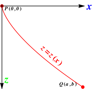
Figure 3: Brachistochrone problem, curve of fastest descent. It is the curve between the two points $P(0,0)$ and $Q(a,b)$ that is covered in the least time by a point particle that starts at $P(0,0)$ with zero kinetic energy and is constrained to move along the curve “Brachistochrone” to $Q(a,b)$, under the action of only constant gravity and assuming no friction.

Let’s start by setting up the co-ordinate system. Suppose that the wire lies in the $(x,z)$-plane with $Pz$ pointing vertically downwards, $P$ at the origin, and $Q$ at the point $(a,b)$. Let the shape of the wire be given by the curve $z=z(x)$. Then, since the particle is released from rest when $z=0$, energy conservation implies that the speed of the particle when its downward displacement is $z$ is given as $v(z)=\sqrt{2gz}$. Then:

$$v(z)=\sqrt{2gz},$$ (77)

$$\Rightarrow v^{2}(z)=2gz,\hskip 125.19212pt\left(\mathrm{squaring\ both\ sides}\right)$$

$$\Rightarrow v_{x}^{2}+v_{z}^{2}=2gz,$$

$$\Rightarrow \left(\frac{dx}{dt}\right)^{2}+\left(\frac{dz}{dt}\right)^{2}=2gz,$$

$$\Rightarrow \left(\frac{dx}{dt}\right)^{2}\left[1+\frac{dz}{dx}\right]^{2}=2gz,$$

$$\Rightarrow (2g)^{-1/2}\frac{\left[1+\dot{z}^{2}\right]}{z^{1/2}}dx=dt\hskip 42.67912pt\left(\mathrm{defining}\ \dot{z}=\frac{dz}{dx}\right).$$

The time, $T$, taken for the particle to complete the transfer is therefore

$$T\left(z(x)\right)=(2g)^{-1/2}\int\limits_{0}^{a}\frac{(1+\dot{z}^{2})^{1/2}}{z^{1/2}}dx.$$ (78)

The problem is to find the function $z(x)$, satisfying the end conditions $z(0)=0$, $z(a)=b$, and that minimizes $T$ [see Fig. (3)]. If $x=x^{*}$ minimizes $T$ , then it must make $T$ stationary and so be an extremized $T$. Since $x$ is not explicitly present in this functional, we can use the integrated form of Eq. (52), $\dot{z}\frac{\partial L}{\partial\dot{z}}-L=0$. Substituting $L(x,z,\dot{z})=\left(1+\dot{z}^{2}\right)^{1/2}/z^{1/2}$ and simplifying we obtain:

$$z\left(1+\dot{z}^{2}\right)=2C,$$ (79)

where $C$ is a positive constant (the constant of integration is called $2C$ for convenience in latter calculations). This equation can be rearranged as

$$\dot{z}=\pm\left(\frac{2C-z}{z}\right)^{1/2},$$ (80)

a pair of first order separable ODEs. Integration gives:

$$x=\pm\int\left(\frac{z}{2C-z}\right)^{1/2}dz.$$ (81)

To perform the integral, we use the substitution $z=C(1-\mathrm{cos}\ \psi)$, in which case

$$x = \pm\int\left(\frac{1-\mathrm{cos}\ \psi}{1+\mathrm{cos}\ \psi}\right)^{1/2}\mathrm{sin}\ \psi\ d\psi$$ (82)

$$= \pm C(\psi-\mathrm{sin}\ \psi)+D,$$

where $D$ is a constant of integration. Hence the parametric form of $z(x)$ that minimize $T(z)$ is

$$x=\pm C(\psi-\mathrm{sin}\ \psi)+D,\hskip 28.45274ptz=C(1-\mathrm{cos}\ \psi).$$ (83)

Here, $C$ and $D$ are two constants that can be fixed by fixing the two points $P$ and $Q$.

5 Relating the Geodesic Equation with Newtonian Gravity

To see that the geodesic equation (68) describes the motion of a particle in a more general theory of gravity than Newton’s gravity, we recover Newton’s second Law of motion as an approximation of Eq. (68). In order to do this, we make following three approximations.

First

The first approximation is the slow motion, non-relativistic ($v\ll c$) one. In this case $\frac{dx^{i}}{d\lambda}\ll\frac{dx^{0}}{d\lambda}$, $\left(\mathrm{or}\ \frac{dx^{i}}{d\lambda}\ll 1\right)$, and the geodesic equation Eq. (68) will take the form (keeping only $\gamma=\delta=0$ terms):

$$\centering\frac{d^{2}x^{\nu}}{d\lambda^{2}}+\Gamma^{\nu}_{00}\frac{dx^{0}}{d\lambda}\frac{dx^{0}}{d\lambda}\@add@centering = 0,$$

$$\Rightarrow\ \ \ \frac{d^{2}x^{\nu}}{d\lambda^{2}}+\Gamma^{\nu}_{00}\left(\frac{dx^{0}}{d\lambda}\right)^{2} = 0.$$ (84)

Second

The second approximation for the metric tensor of spacetime is the weak field approximation (nearly flat spacetime). In this case, we write

$$g_{\mu\nu}(x)=\eta_{\mu\nu}+h_{\mu\nu}(x),$$ (85)

where $\eta_{\mu\nu}$ is the Minkowski (flat) spacetime metric tensor, and $h_{\mu\nu}(x)$ is a small perturbation $\left(|h_{\mu\nu}(x)|\ll 1\right)$ that depends only on position.

Since the components of the correction tensor $h_{\mu\nu}$ are small, we can use $\eta_{\mu\nu}$, and its inverse to raise and lower indices without including any $h_{\mu\nu}$ term. We will need $g^{\mu\nu}(x)\approx\eta^{\mu\sigma}-h^{\mu\sigma}$, justified as follows,

$$g_{\mu\nu}g^{\mu\sigma} = g_{\mu\nu}\left(\eta^{\mu\sigma}-h^{\mu\sigma}\right),$$ (86)

$$= \left(\eta_{\mu\nu}+h_{\mu\nu}\right)\left(\eta^{\mu\sigma}-h^{\mu\sigma}\right),$$

$$= \eta_{\mu\nu}\eta^{\mu\sigma}-\eta_{\mu\nu}h^{\mu\sigma}+h_{\mu\nu}\eta^{\mu\sigma}-\underbrace{h_{\mu\nu}h^{\mu\sigma}}_{O[h^{2}]\rightarrow\mathrm{Neglect}},$$

$$\approxeq \delta_{\nu}^{\sigma}-\eta_{\mu\nu}h^{\mu\sigma}+h_{\mu\nu}\eta^{\mu\sigma}.$$

Let’s consider the last term of Eq. (86):

$$h_{\mu\nu}\eta^{\mu\sigma} = \left(\eta_{\nu\rho}h_{\mu}^{\rho}\right)\left(\eta^{\sigma\lambda}\eta_{\lambda}^{\mu}\right),$$ (87)

$$= \eta_{\nu\rho}\eta^{\sigma\lambda}h_{\mu}^{\rho}\eta_{\lambda}^{\mu},$$

$$= \eta_{\nu\rho}\eta^{\sigma\lambda}\left(\eta_{\alpha\mu}h^{\alpha\rho}\right)\left(\eta^{\alpha\mu}\eta_{\alpha\lambda}\right),$$

$$= \eta_{\nu\rho}\eta^{\sigma\lambda}\underbrace{\left(\eta_{\alpha\mu}\eta^{\alpha\mu}\right)}_{=1}\left(h^{\alpha\rho}\eta_{\alpha\lambda}\right),$$

$$= \eta_{\nu\rho}\underbrace{\left(\eta^{\sigma\alpha}\eta_{\alpha\lambda}\right)}_{=\delta_{\alpha}^{\sigma}}h^{\alpha\rho},$$

$$= \eta_{\nu\rho}\delta_{\alpha}^{\sigma}h^{\alpha\rho},$$

$$= \eta_{\nu\rho}h^{\sigma\rho},$$

$$= \eta_{\nu\mu}h^{\mu\sigma}.$$

Hence, from Eq. (86) and Eq. (87) we can see $g_{\mu\nu}\left(\eta^{\mu\sigma}-h^{\mu\sigma}\right)=\delta_{\nu}^{\sigma}$:

$$\Rightarrow g^{\mu\nu}(x)=\eta^{\mu\nu}-h^{\mu\nu}(x).$$ (88)

Third

The third approximation is the time independence of the perturbation. We will consider $h_{\mu\nu}(x)$ to be the time independent, i.e.

$$\partial_{0}{h_{\mu\nu}(x)}=\frac{\partial h_{\mu\nu}(x)}{\partial x^{0}}=\frac{\partial h_{\mu\nu}(x)}{\partial t}=0.$$ (89)

We now compute the Christoffel symbol in Eq. (84) under the second and third approximation and the definition in Eq. (36) we have:

$$\Gamma^{\nu}_{00} \equiv \frac{1}{2}g^{\nu\gamma}\Big{(}g_{0\gamma,0}+g_{\gamma 0,0}-g_{00,\gamma}\Big{)}.$$ (90)

Because of the stationary field approximation $\left(g_{\alpha\beta,0}=0\right)$, this becomes

$$\Gamma^{\nu}_{00} = -\frac{1}{2}g^{\nu\alpha}g_{00,\alpha}=-\frac{1}{2}g^{\nu i}g_{00,i}.$$ (91)

From Eq. (85)

$$g_{\alpha\beta,i}(x)=\eta_{\alpha\beta,i}+h_{\alpha\beta,i}(x)=h_{\alpha\beta,i}(x).\hskip 14.22636pt\left(\mathrm{since}\ \eta_{\alpha\beta,i}=0\right)$$ (92)

Eqs. (88), (90), and (92), lead to:

$$\Gamma^{\nu}_{00} = -\frac{1}{2}g^{\nu i}h_{00,i}$$ (93)

$$= -\frac{1}{2}\left(\eta^{\nu i}-h^{\nu i}\right)h_{00,i}$$

$$= -\frac{1}{2}\eta^{\nu i}h_{00,i}+\underbrace{\frac{1}{2}h^{\nu i}h_{00,i}}_{O^{2}(h)\rightarrow\mathrm{Neglect~{}it}}.$$

Since $\Gamma_{00}^{0}=0$, Eqs. (84) and (93), gives the geodesic equation as

$$\frac{d^{2}x^{j}}{d\lambda^{2}} = \frac{1}{2}\eta^{ji}h_{00,i}\left(\frac{dx^{0}}{d\lambda}\right)^{2}.$$ (94)

Now

$$\frac{dx^{j}}{d\lambda} = \frac{dx^{j}}{dt}\frac{dt}{d\lambda},$$

$$\frac{d^{2}x^{j}}{d\lambda^{2}} = \frac{d}{d\lambda}\left(\frac{dx^{j}}{dt}\frac{dt}{d\lambda}\right)=\frac{d}{dt}\left(\frac{dx^{j}}{dt}\frac{dt}{d\lambda}\right)\frac{dt}{d\lambda}=\frac{d^{2}x^{j}}{dt^{2}}\left(\frac{dt}{d\lambda}\right)^{2}.$$ (95)

So the geodesic equation becomes

$$\frac{d^{2}x^{j}}{dt^{2}}=\frac{1}{2}\eta^{ji}h_{00,i}.$$ (96)

Recalling that $x^{j}=(x,y,z)$, and expressing it in vector format, we arrive at

$$\frac{d^{2}\vec{x}}{dt^{2}} = \frac{1}{2}\vec{\nabla}h_{00}(\vec{x})=\vec{\nabla}\left(\frac{h_{00}(\vec{x})}{2}\right).$$ (97)

When we compare this to Newton’s second Law

$$\frac{d^{2}\vec{x}}{dt^{2}} = -\vec{\nabla}\Phi,$$ (98)

we see that

$$h_{00} = -2\Phi.$$ (99)

Hence $g_{00}=\eta_{00}+h_{00}=-1-2\Phi$. In a spherically symmetric situation $\Phi=-\frac{GM}{r}$, so

$$g_{00} = -\left(1-\frac{2GM}{r}\right),$$ (100)

where $G$ is the Newtonian gravitational constant. Thus, if mass $M$ is small or we are far away from mass $M$ then $g_{00}\approx-1$ like in Minkowski spacetime, and hence time and proper time are indistinguishable in the Newtonian limit. Equation (100) quantifies how mass curves spacetime in the Newtonian approximation. Hence the geodesic equation is the general relativity equivalent of Newton’s Laws. This describes how a particle moves in a curved spacetime, like Newton’s second Law describes how a particle moves under the action of a force.

3 Einstein’s Field Equation

Einstein’s field equation, the general relativity generalization of Poisson’s equation for gravity, is a set of 10 equations that governs gravity. In Albert Einstein’s general theory of relativity, which describes the fundamental interaction of gravitation as a result of spacetime being curved by matter and energy.¹²⁰ First published by Einstein in 1915 as a tensor equation, the Einstein field equation equates local spacetime curvature (expressed by the Einstein tensor $G_{\mu\nu}$) to the local energy and momentum within that spacetime (expressed by the stress-energy tensor $T_{\mu\nu}$).

Similar to the way that electromagnetic fields are determined from the source charges and currents through Maxwell’s equations, Einstein’s field equations are used to determine the spacetime geometry resulting from the presence of mass-energy and linear momentum (sources), that is, they determine the metric tensor of spacetime for a given arrangement of stress-energy in the spacetime. The relation between the metric tensor and the Einstein tensor allows the Einstein field equation to be written as a set of non-linear partial differential equations. The solutions of the Einstein field equation are the components of the metric tensor. The inertial trajectories (geodesics) of particles and radiation in the resulting geometries are then calculated using the geodesic equation.⁸⁰

1 Riemann Tensor, Ricci Tensor, Ricci Scalar, Einstein Tensor

Riemann (curvature) tensor

The Riemann curvature tensor, or Riemann-Christoffel tensor, is the most common tensor used to describe the curvature of Riemannian manifolds. It associates a tensor to each point of a Riemannian manifold (i.e., it is a tensor field) that measures the extent to which the metric tensor is not locally isometric to a Euclidean flat space and so specifies the geometrical properties of spacetime. More precisely, the Riemann tensor governs the evolution of a vector on a displacement parallel propagated along a geodesic.¹⁰² It is defined in terms of Christoffel symbols as

$$R^{\alpha}_{\beta\gamma\delta}\equiv\Gamma^{\alpha}_{\beta\delta,\gamma}-\Gamma^{\alpha}_{\beta\gamma,\delta}+\Gamma^{\nu}_{\beta\delta}\Gamma^{\alpha}_{\nu\gamma}-\Gamma^{\nu}_{\beta\gamma}\Gamma^{\alpha}_{\nu\delta},$$ (101)

where $\Gamma^{\alpha}_{\beta\delta,\gamma}\equiv\frac{\partial\Gamma^{\alpha}_{\beta\delta}}{\partial x^{\gamma}}$. The spacetime is considered flat if the Riemann tensor vanishes everywhere. The Riemann tensor can also be written directly in terms of the spacetime metric

$$R_{\alpha\beta\gamma\delta}\equiv\frac{1}{2}\left(g_{\beta\gamma,\alpha\delta}+g_{\alpha\delta,\beta\gamma}-g_{\beta\delta,\alpha\gamma}-g_{\alpha\gamma,\beta\delta}\right)+g_{\mu\nu}\Gamma^{\nu}_{\alpha\gamma}\Gamma^{\mu}_{\beta\delta}-g_{\mu\nu}\Gamma^{\nu}_{\alpha\delta}\Gamma^{\mu}_{\beta\gamma}.$$ (102)

The Riemann tensor has the following symmetries.

Skew symmetry

$$R_{\alpha\beta\gamma\delta}=-R_{\beta\alpha\gamma\delta}=-R_{\alpha\beta\delta\gamma}.$$ (103)

Interchange symmetry:

$$R_{\alpha\beta\gamma\delta}=R_{\gamma\delta\alpha\beta},$$ (104)

First Bianchi identity

$$R_{\alpha\beta\gamma\delta}+R_{\alpha\gamma\delta\beta}+R_{\alpha\delta\beta\gamma}=0,$$ (105)

which is often written as:

$$R_{\alpha[\beta\gamma\delta]}=0.$$ (106)

Because of the symmetries above, the Riemann tensor in 4-dimensional spacetime has only 20 independent components out of $4^{4}=256$. The general rule for computing the number of independent components in an $N$-dimensional spacetime is $N^{2}\left(N^{2}-1\right)/12$.³⁶

Second Bianchi identity

$$R_{\alpha\beta\gamma\delta;\nu}+R_{\alpha\beta\nu\gamma;\delta}+R_{\alpha\beta\delta\nu;\gamma}=0,$$ (107)

which can be written as

$$R_{\alpha\beta[\gamma\delta;\nu]}=0,$$ (108)

Raising two indices we have,

$$R^{\alpha\beta}_{[\gamma\delta;\nu]}=0.$$ (109)

Setting $\gamma=\alpha$ and $\delta=\beta$, we get

$$R^{\alpha\beta}_{[\alpha\beta;\nu]} = 0,$$

$$\Rightarrow\ \ R^{\alpha\beta}_{\alpha\beta;\nu}+R^{\alpha\beta}_{\beta\nu;\alpha}+R^{\alpha\beta}_{\nu\alpha;\beta} = 0,$$

$$\Rightarrow\ \ R^{\alpha\beta}_{\alpha\beta;\nu}-R^{\alpha\beta}_{\nu\beta;\alpha}+R^{\alpha\beta}_{\alpha\nu;\beta} = 0,$$

$$\Rightarrow\ \ \mathcal{R}_{;\nu}-R^{\alpha}_{\nu;\alpha}+R^{\beta}_{\nu;\beta} = 0,$$

$$\Rightarrow\ \ 2R^{\alpha}_{\nu;\alpha} = \mathcal{R}_{;\nu},$$ (110)

which after raising the index is,

$$R^{\alpha\beta}_{;\alpha}=\frac{1}{2}g^{\alpha\beta}\mathcal{R}_{;\alpha}.$$ (111)

Here $\mathcal{R}$ is Ricci scalar, discuss below. We will use Eq. (111) in Sec. (6).

Ricci tensor

The Ricci tensor, or the Ricci curvature tensor, governs the evolution of a small volume parallel propagated along a geodesic.¹⁰² It is obtained from the Riemann tensor by contracting over two of the indices,

$$R_{\alpha\beta}\equiv R^{\gamma}_{\alpha\gamma\beta}.$$ (112)

It is symmetric, which means that it has at most 10 independent components out of $4\times 4=16$. For the case of vacuum we will see later, the field equation is $R_{\mu\nu}=0$.

Ricci scalar

The Ricci scalar $\mathcal{R}$ is obtained by contracting the Ricci tensor over the remaining two indices and is denoted by :

$$\mathcal{R}\equiv g^{\alpha\beta}R_{\alpha\beta}=R^{\alpha}_{\alpha}.$$ (113)

Einstein tensor

The Einstein tensor is defined in terms of the Ricci tensor and Ricci scalar as

$$G_{\alpha\beta}\equiv R_{\alpha\beta}-\frac{1}{2}g_{\alpha\beta}\mathcal{R}.$$ (114)

One can use Eq. (111) to derive a very important property of the Einstein tensor, $G_{\alpha\beta;\alpha}=0$.

2 Energy-Momentum Tensor

In the Newtonian approximation, the gravitational field is directly proportional to mass. In general relativity, mass is just one of several sources of spacetime curvature. The energy-momentum (stress-energy) tensor, denoted by $T^{\mu\nu}$, includes all possible forms of sources (energy) that can curve spacetime, and it describes the density and flow of the 4-momentum $(-E,p_{\mathrm{x}},p_{\mathrm{y}},p_{\mathrm{z}},)$.¹¹¹ In simple terms, the stress-energy tensor quantifies all the stuff that causes spacetime to curve, and thus to the gravitational field. More rigorously, the components $T^{\mu\nu}$ of the stress-energy tensor is the flux of the $\mu$ component of the four momentum crossing the surface of constant $x^{\nu}$. A surface of constant $x^{\nu}$ is simply a 3-plane perpendicular to the $x^{\nu}$-axis. Hence, the stress-energy tensor is the flux of a 4-momentum across a surface of a constant coordinate. In other words, the stress-energy tensor describes the density of energy and momentum and the flux of energy and momentum in a region. Since, under the mass-energy equivalence principle, we can convert mass units to energy units and vice-versa, then the stress-energy tensor can describe all the mass and energy in a given region of spacetime. In simple layman’s language, the stress-energy tensor represents everything that gravitates.

The stress-energy tensor, being a tensor of rank two in four-dimensional spacetime, has sixteen components that can be written as a 4$\times$4 matrix, and has the following structure in an orthonormal basis

$$T^{\mu\nu}=\left({\begin{array}[]{cccc}{\color[rgb]{0,0,1}T^{00}}&{\color[rgb]{1,0,0}T^{01}}&{\color[rgb]{1,0,0}T^{02}}&{\color[rgb]{1,0,0}T^{03}}\\ {\color[rgb]{1,0,1}T^{10}}&{\color[rgb]{0,1,0}T^{11}}&{\color[rgb]{0,1,1}T^{12}}&{\color[rgb]{0,1,1}T^{13}}\\ {\color[rgb]{1,0,1}T^{20}}&{\color[rgb]{0,1,1}T^{21}}&{\color[rgb]{0,1,0}T^{22}}&{\color[rgb]{0,1,1}T^{23}}\\ {\color[rgb]{1,0,1}T^{30}}&{\color[rgb]{0,1,1}T^{31}}&{\color[rgb]{0,1,1}T^{32}}&{\color[rgb]{0,1,0}T^{33}}\\ \end{array}}\right).$$ (115)

• Here $T^{00}=T^{tt}$, represents the energy flow $p^{0}$, crossing a hypersurface of constant time $(x^{0}=t)$. A hypersurface of constant time is the volume. Hence, $T^{00}$ is the energy density.

• $T^{0i}$ represents the flow (flux) of energy in the $x^{i}$ direction.

• $T^{i0}$ represents the $i-$component of the momentum density.

• $T^{ij}$ ($i\neq j$) represents the flow of the $i-$component of momentum in the $j-$direction (shear stress, i.e., stress applied tangential to the region).

• $T^{ii}$ represents the components of normal stress, or stress applied perpendicular to the region (normal stress is another term for pressure).

Note that the components $T^{00}$, $T^{10}$, $T^{20}$ and $T^{30}$ are interpreted as densities. A density is what you get when you measure the flux of 4-momentum across a 3-surface of constant time, which means the instantaneous value of 4-momentum flux is density.

To develop more insight of the energy-momentum tensor, let’s consider the example of a cylinder with a piston that is fixed and cannot move, hence the volume of the cylinder is fixed. Initially we consider that the pressure of the air inside and outside is the same, which means that no net force acts on the walls of the cylinder. If we now heat the cylinder, the temperature of the air inside will increase according to the ideal gas law. The mass of the cylinder will remain the same, but the energy content inside the box has increased due to the extra kinetic energy given to the molecules of the air inside the cylinder during the process of heating. This will increase the time-time component of the stress-energy tensor $T^{00}$ and consequently increase the spacetime curvature around the cylinder. It is against our intuition that just by increasing the pressure inside the cylinder it will make it heavier and cause spacetime to curve more around the cylinder. This is because, in daily life, the contribution of increased pressure and kinetic energy on the gravitational effect of the cylinder is negligible, as compared to the mass contribution, and our intuition is developed on the basis of daily life experience. Hence, it is our intuition that needs to be blamed, and we should consider it wrong. On larger scales, such as the sun, pressure and temperature contribute significantly to the gravitational field.

We can see that the stress-energy tensor neatly quantifies all static and dynamic properties of a region of spacetime, from mass to momentum to temperature to pressure to shear stress. This is the only mathematical quantity that we want to know about a particular region of space to find its gravitational effects.

A very good proof that stress-energy tensor is symmetric $\left(T^{\mu\nu}=T^{\nu\mu}\right)$, is given in Gravitation¹¹¹ on page 141. Hence, it has only 10 independent components. The conservation equation (which incorporates both energy and momentum conservation in a general metric)

$$T^{\mu\nu}_{;\nu}=0.$$ (116)

In the limit of flat spacetime (Minkowski metric), the covariant derivative reduced to an ordinary derivative and we will get:

$$\frac{\partial T^{\mu\nu}}{\partial x^{\nu}}=0.$$ (117)

For $\mu=0=t$, one finds the continuity equation for energy conservation as:

$$\frac{\partial T^{tt}}{\partial t}+\frac{\partial T^{it}}{\partial x^{i}}=\frac{\partial\varepsilon}{\partial t}+\vec{\nabla}\cdot\vec{J}=0,$$ (118)

where $\varepsilon=T^{tt}$ and $J^{i}=T^{it}$ are the energy and momentum densities respectively.

We now consider three types of energy-momentum tensors frequently used in GR: classical vacuum, dust and perfect fluid.

Vacuum: This is the simplest possible stress-energy tensor in which all the values are zero:

$$T^{\mu\nu}=0.$$ (119)

This tensor represents a region of space in which there is no matter, energy, or fields. This is not just at a given instant, but over the entire period of time in which we’re interested in. Nothing exists in this region, and nothing happens in this region.

So one might assume that in a region where the stress-energy tensor is zero, the gravitational field must also necessarily be zero. There’s nothing there to gravitate, so it follows naturally that there can be no gravitation. In fact, it’s not that simple. For details see van Nieuwenhove.¹⁷⁶

Dust: Imagine a time-dependent distribution of identical, massive, non-interacting, electrically neutral particles. In general relativity, such a distribution is called a dust. Let’s break down what this means.

• Time-dependent: The distribution of particles in dust is not a constant; that is to say, the particles may be in motion. The overall configuration you see when you look at the dust depends on the time at which you look at it, so the dust is said to be time-dependent.

• Identical: The particles that make up dust are all exactly the same; they don’t differ from each other in any way.

• Massive: Each particle in dust has some rest mass. Because the particles are all identical, their rest masses must also be identical. We’ll call the rest mass of an individual particle $m_{0}$.

• Non-interacting: The particles don’t interact with each other in any way; they don’t collide, and they don’t attract or repel each other. This is, of course, an idealization; since the particles have mass $m_{0}$, they must at least interact with each other gravitationally, if not in other ways. However, we’re constructing our model in such a way that gravitational effects between the individual particles are so small they can be neglected. Either the individual particles are very tiny, the average distance between them is very large, or may be both.

• Electrically neutral: In addition to the obvious electrostatic effect of two charged particles either attracting or repelling each other, violating our “non-interacting” assumption, allowing the particles to be both charged and in motion would introduce electrodynamic effects that would have to be included in the stress-energy tensor. We prefer to ignore these effects for the sake of simplicity, so by definition, the particles in dust are all electrically neutral.

To fully describe the dust we need to write its energy-momentum tensor, which is given by

$$T^{\mu\nu}=\rho u^{\mu}u^{\nu}.$$ (120)

For a comoving observer, the 4-velocity is given by $\vec{u}=(1,0,0,0)$, so the stress-energy tensor reduces to

$$T^{\mu\nu}=\left({\begin{array}[]{cccc}\rho&0&0&0\\ 0&0&0&0\\ 0&0&0&0\\ 0&0&0&0\\ \end{array}}\right).$$ (121)

Dust is an approximation to the content of the Universe at later times, when radiation is negligible.

Perfect fluid: It is a fluid that has no heat conduction or viscosity. It is fully parametrized by its mass density $\rho$ and the pressure $P$ . The stress-energy tensor is given by

$$T^{\mu\nu}=\left(\rho+P\right)u^{\mu}u^{\nu}+Pg^{\mu\nu}.$$ (122)

For a comoving observer, the 4-velocity is $\vec{u}=(1,0,0,0)$, so the stress-energy tensor reduces to

$$T^{\mu\nu}=\left({\begin{array}[]{cccc}\rho&0&0&0\\ 0&P&0&0\\ 0&0&P&0\\ 0&0&0&P\\ \end{array}}\right).$$ (123)

In the limit as $P\rightarrow 0$, the perfect fluid approximation reduces to that of dust. A perfect fluid can be used an approximation to the components of the Universe at earlier times, when radiation dominates.

3 Conservation Laws and Energy Evolution

Stress-Energy conservation, Eq. (116), can be used to determine how components of the energy-momentum tensor evolve with time. Considering the special case of perfect fluid, and using Eq. (123) and Eq. (14), the mixed energy-momentum tensor is

$$T^{\mu}_{\nu}=\left({\begin{array}[]{cccc}-\rho&0&0&0\\ 0&P&0&0\\ 0&0&P&0\\ 0&0&0&P\\ \end{array}}\right),$$ (128)

and the four conservation equations using Eq. (40) are

$$T^{\mu}_{\nu;\mu}\equiv\frac{\partial T^{\mu}_{\nu}}{\partial x^{\mu}}+\Gamma^{\mu}_{\alpha\mu}T^{\alpha}_{\nu}-\Gamma^{\alpha}_{\nu\mu}T^{\mu}_{\alpha}=0.$$ (129)

Consider the $\nu=0$ equations

$$\frac{\partial T^{\mu}_{0}}{\partial x^{\mu}}+\Gamma^{\mu}_{\alpha\mu}T^{\alpha}_{0}-\Gamma^{\alpha}_{0\mu}T^{\mu}_{\alpha}=0.$$ (130)

As a consequence of the isotropy, assumed as the fundamental principle of cosmology, all non-diagonal terms of $T^{\mu\nu}$ vanish (i.e., $T^{\mu\nu}=0$ if $\mu\neq\nu$), hence $T^{i}_{0}=0$. This means that $\mu=0$ in the first term of Eq. (130) and $\alpha=0$ in the second term, and Eq. (130) becomes

$$\frac{\partial T^{0}_{0}}{\partial x^{0}}+\Gamma^{\mu}_{0\mu}T^{0}_{0}-\Gamma^{\alpha}_{0\mu}T^{\mu}_{\alpha}=0.$$ (131)

From Eq. (128), $T^{0}_{0}=-\rho$, so we have

$$\frac{\partial\rho}{\partial t}+\Gamma^{\mu}_{0\mu}\left(\rho+T^{\mu}_{\alpha}\right) = 0.$$ (132)

Now, we need to calculate the Christoffel symbol $\Gamma^{\mu}_{0\mu}$. For simplicity we consider expanding flat space-time with the flat Friedman-Lemaître-Robertson-Walker metric tensor given by Eq. (28): The Christoffel symbols are given by Eq. (36). To start, let’s put $\beta=0$ in Eq. (39) to get $\Gamma^{\alpha}_{0\mu}$:

$$\Gamma^{\alpha}_{0\mu}=\frac{1}{2}g^{\alpha\gamma}\Big{(}g_{\gamma 0,\mu}+g_{\mu\gamma,0}-g_{0\mu,\gamma}\Big{)}.$$ (133)

But $g_{\gamma 0}$ and $g_{0\mu}$ are constants and hence $g_{\gamma 0,\mu}=g_{0\mu,\gamma}=0$

$$\Gamma^{\alpha}_{0\mu}=\frac{1}{2}g^{\alpha\gamma}g_{\mu\gamma,0}.$$ (134)

Let’s figure out its components:

• when $\alpha=\mu=0$:

  $$\Gamma^{0}_{00}=\frac{1}{2}g^{0\gamma}g_{0\gamma,0}=0.\hskip 19.91692pt\left(\because\ g_{0\gamma,0}=0\right)$$ (135)

• when $\alpha=\mu=i$, where $i\in\left\{1,2,3\right\}$:

  $$\Gamma^{i}_{0i} = \frac{1}{2}g^{i\gamma}g_{i\gamma,0},$$ (136)

  $$= \frac{1}{2}\left(g^{i1}g_{i1,0}+g^{i2}g_{i2,0}+g^{i3}g_{i3,0}\right),$$

  $$= \frac{1}{2}\left(g^{i1}+g^{i2}+g^{i3}\right)\left(g_{i1,0}\right),\hskip 19.91692pt\left(\because\ g_{\mu\nu}\ \mathrm{is\ diagonal}\right)$$

  $$= \frac{1}{2}\left(\frac{1}{a^{2}}+\frac{1}{a^{2}}+\frac{1}{a^{2}}\right)(2a\dot{a}),$$

  $$= 3\frac{\dot{a}}{a}.$$

• when $\alpha=i$, $\mu=j$ and  $i\neq j$:

  $$\Gamma^{j}_{0i}=\frac{1}{2}g^{j\gamma}g_{i\gamma,0}=0.$$ (137)

Hence, we can conclude:

$$\Gamma^{\mu}_{0\mu}=\Gamma^{i}_{0i}=3\frac{\dot{a}}{a}.$$ (138)

So the conservation laws in an expanding Universe, Eq. (132), takes the form

$$\hskip 14.22636pt-\frac{\partial\rho}{\partial t}-3\frac{\dot{a}}{a}\rho-\frac{\dot{a}}{a}T^{i}_{i}=0,$$

$$\hskip 14.22636pt\frac{\partial\rho}{\partial t}+3\frac{\dot{a}}{a}\rho+\frac{\dot{a}}{a}\left(3P\right)=0,$$

$$\hskip 14.22636pt\frac{\partial\rho}{\partial t}=-3\frac{\dot{a}}{a}\left(\rho+P\right).$$ (139)

Here $a(t)$ is the cosmological scale factor and an over-dot denotes a derivative with respect to cosmological time.

For a perfect fluid the equation-of-state, which is the relationship between pressure $P$ and the density $\rho$ of the fluid is:

$$P=\rho\ \omega.$$ (140)

Using the equation of state, Eq. (139) takes the form:

$$\frac{\partial\rho}{\partial t} = -3\ \rho\left(\frac{\dot{a}}{a}\right)\left(1+\omega\right).$$ (141)

This is separable first order ordinary differential equation with the solution

$$\rho(t)=\rho_{0}\left(\frac{a_{0}}{a}\right)^{3(1+\omega)}.$$ (142)

Here $\rho_{0}$ is the density of matter at scale factor $a_{0}$, which we take to be the value today. We can assume $a_{0}=1$ without loss of generality.

Equation (142) describes the evolution of a particular kind of species whose time-dependent energy density is $\rho$, with equation-of-state parameter $\omega$. Now let’s consider different kinds of energy densities and their evolution according to Eq. (142):

• For cold matter (dust), we have zero pressure, $P_{m}=0$, so $\omega_{m}=0$ and

  $$\rho_{m}(t)\propto\frac{1}{a^{3}}.$$ (143)

  This should come as no surprise, because the total amount of matter is conserved, and the volume of the Universe goes as $V\propto a^{3}$, hence, $\rho\propto\frac{1}{V}\propto a^{-3}$.

• For radiation $P_{r}=\frac{1}{3}\rho_{r}$, so $\omega_{r}=\frac{P_{r}}{\rho_{r}}=\frac{1}{3}$. This means that:

  $$\rho_{r}(t)\propto\frac{1}{a^{4}}.$$ (144)

  This too should not surprise us — since radiation density is directly proportional to the energy per particle and inversely proportional to the total volume, i.e., $\rho_{r}\propto\frac{\hbar\nu}{V}\propto\frac{\hbar}{\lambda V}\propto a^{-4}$, because $\lambda\propto a$. The last part states that the energy per particle decreases as the Universe expands.

• For the case of curvature where $\omega_{k}=-\frac{1}{3}$, using Eq. (142) we find

  $$\rho_{k}(t)\propto\frac{1}{a^{2}},$$ (145)

  where $\rho_{k}$ is the time-dependent energy density corresponding to the space curvature of the Universe.

Now, we are ready to postulate Einstein’s field equation.

4 Einstein’s Field Equation

Just as Maxwell’s equations govern the electric and magnetic field response to electric charges and current (sources), Einstein’s field equations describe how the metric is governed by energy and momentum (sources).

The general relativity must describe both parts of the dynamical picture. ³⁶

• How gravity affects the motion of particles (i.e., how force is applied on the particle, when it is placed in the gravitational field).

• How the gravitational field is generated by a source of mass energy.

The first part is described by the geodesic equation, derived in Sec. (4):

$$\frac{d^{2}x^{\nu}}{d\lambda^{2}}+\Gamma^{\nu}_{\gamma\delta}\frac{dx^{\gamma}}{d\lambda}\frac{dx^{\delta}}{d\lambda}=0,$$ (146)

which is analogous to Newton’s second law of motion $\vec{F}=m\vec{a}$.

The second part requires finding the analog of the Poisson equation

$$\nabla^{2}\Phi(\vec{x})=4\pi G\rho(\vec{x}),$$ (147)

which specifies how matter (or energy in general relativity) curves spacetime. Here $\nabla^{2}=\delta^{ij}\partial_{i}\partial_{j}$ is the Laplacian in space and $\rho$ is the mass density [the explicit form of $\phi=-GM/r$ is the solution of Eq. (147) for the case of a spherically symmetric mass distribution].

In classical Newtonian gravity, gravitational effects are produced by the mass at rest. In modified Newtonian gravity, which we can call special relativity, we learned that rest mass is also a form of energy; thus special relativity put mass and energy on equal footing. Extending this idea, one should expect that in general relativity, all sources of both energy and momentum contribute in generating spacetime curvature. On the left hand side of Eq. (147) we have a second order differential operator acting on the gravitational potential and on the right hand side we have the measure of mass density. The relativistic generalization of the Poisson equation should be the relationship between tensors. The tensor generalization of mass density can be $T^{\mu\nu}$. This means that we consider the stress-energy tensor $T^{\mu\nu}$ as the source of spacetime curvature (with an unknown scaling factor), in the same sense that the mass density $\rho$ is the source for the potential $\Phi$ in Newtonian gravity. Hence, the right hand side of the general relativity analog of the Poisson equation should be $\kappa T^{\mu\nu}$ (where $\kappa$ is an unknown constant to be determined latter.)

As far as the left hand side of general relativity analog of the Poisson equation, we have seen earlier in Eq. (100), the spacetime metric in the Newtonian limit is modified by a term that is proportional to $\Phi$. Extending this idea, the general relativity counterpart of $\nabla^{2}\Phi(\vec{x})$ would contain terms having the second derivative of the metric tensor. Something along the lines of:

$$\Big{[}\nabla^{2}\ g\Big{]}_{\mu\nu}=\kappa T^{\mu\nu}.$$ (148)

But of course we want it to be completely tensorial and the left-hand side of Eq. (148) is not a tensor. It is just simplistic notation that indicates we need something on the left hand side that should have the second derivative of the metric.

The Riemann tensor $R_{\alpha\beta\gamma\delta}$, and consequently its contractions, the Ricci tensor $R_{\alpha\beta}=R^{\gamma}_{\alpha\gamma\beta}$, and the Ricci scalar $\mathcal{R}=R^{\alpha}_{\alpha}$, contain the second derivative of the metric and therefore is a candidate for the left hand side of Einstein’s field equations.

Following this line of thought, Einstein originally suggested that the field equations might be

$$R_{\mu\nu}=\kappa T_{\mu\nu},$$ (149)

but one can see directly that this can not be correct. While the conservation of energy and momentum require $T^{\mu\nu}_{;\mu}=0$, the same in general is not true for the Ricci tensor $R^{\mu\nu}_{;\mu}\neq 0$. However Einstein’s tensor, $G_{\mu\nu}=R_{\mu\nu}-\frac{1}{2}g_{\mu\nu}\mathcal{R}$, which is a combination of the Ricci tensor and scalar, satisfies the divergence-less condition $\nabla^{\mu}G_{\mu\nu}=0$, see Eq. (111). Therefore, Einstein’s field equation becomes

$$G_{\mu\nu}\equiv R_{\mu\nu}-\frac{1}{2}g_{\mu\nu}\mathcal{R}=\kappa T_{\mu\nu}.$$ (150)

This equation satisfies all of the obvious requirements: the right-hand side of is a covariant expression of the energy and momentum density in the form of a symmetric and conserved tensor, while the left-hand side is also a symmetric and conserved tensor constructed from the first and second derivatives of the metric tensor and the metric tensor itself. The only issue that remains is to fix the constant $\kappa$. By matching Einstein’s equation in the Newtonian limit to the Poisson equation, the constant $\kappa$ was found to $8\pi G$, where $G$ is the Newtonian gravitational constant. Then Eq. (150) takes the form

$$G_{\mu\nu}\equiv R_{\mu\nu}-\frac{1}{2}g_{\mu\nu}\mathcal{R}=8\pi GT_{\mu\nu}.$$ (151)

Summarizing, Einstein’s equations for the gravitational field came from requiring that the equations of motion were generally covariant under coordinate transformations and reduced to the Newtonian form in weak stationary gravitational fields. The field equation relates the Ricci tensor, that is made up of second derivatives of the metric tensor, to the Ricci scalar formed by contracting the Ricci tensor, and to the energy-momentum content of the Universe. Remember, this is not the proof of the field equations.

4 Hubble’s Law and Redshift of Distant Galaxies

In 1912 Slipher discovred most nearby galaxies were moving away and measured their velocities $v$, but he did not know they were galaxies. Hubble⁸² showed they were galaxies in 1925-26 and measured distance $r$ and showed in 1929

$$v\propto r,$$ (152)

This phenomenon was observed as a redshift of a galaxy’s spectrum. This redshift appeared to have a larger value for fainter, presumably farther away, galaxies. Hence, the farther a galaxy, the faster it is receding from Earth. Consider two galaxies separated by the distance $r$, then the relative velocity $v\propto r$, this is called Hubble’s law and mathematically given as

$$\vec{v}=H_{0}\vec{r},$$ (153)

where, $H_{0}$ is Hubble constant that relates the distance of the galaxy (for the earth based observers this is conveniently taken to be the distance from our galaxy) to its recession velocity. The Hubble constant $H_{0}$ is one of the most important numbers in cosmology, because it may be used to estimate the size of the observable Universe and its age. It indicates the rate at which the Universe is expanding. Since more generally a related law holds at all times, $\vec{v}(t)=H(t)\vec{r}(t)$ where Eq. (153) $H(t)$ is the Hubble parameter whose current value is the Hubble constant $H(t_{0})=H_{0}$.

The units of the Hubble constant (or parameter) are kilometers per second per megaparsec. In other words, for each megaparsec of distance, the velocity of a distant object appears to increase by some value. For example, if the Hubble constant was determined to be 65 kms^-1 Mpc^-1, a galaxy at 10 Mpc would have a redshift corresponding to a radial recession velocity of 650 kms^-1.

The reasonable current summary value of Hubble constant is $H\pm\sigma_{H_{0}}=68\pm 2.8$ kms^-1 Mpc^-1. ^{43, 40}

The discovery of Hubble’s Law marked the commencement of the era of quantitative cosmology in which theories of the Universe could be subject to observational test. Since the days of Hubble, advances in technology have enabled astronomers to measure the light from increasingly deeper space and more ancient time, and our ideas of the entire history of the expanding universe have been gradually converging into a unified picture called the Big Bang—model.

At first glance, it looks like Hubble’s law is a violation of cosmological principle, because all galaxies are moving away from us, which might seen to put us in a special location in the Universe. In fact, what we see here in our Galaxy exactly what you would be expected in a Universe which is undergoing homogeneous and isotropic expansion. We see distant galaxies moving away from us; but observers in any other galaxy would also see distant galaxies moving away from them.

Let’s define some terminologies:

Physical or proper distance: The actual distance between the two points in space is called the physical distance. It is denoted by $\vec{r}(t)$.

Comoving or coordinate distance: This is just the label of the point in space and it is independent of time. It is denoted by $\vec{x}$

The physical and comoving distance: are related through

$$\vec{r}(t)=a(t)\ \vec{x},$$ (154)

where $a(t)$ is called the scale factor, a time dependent scalar that describes the the expansion (or contraction) of the Universe. Scale factor $a(t)$ is a dimensionless function of time that carries important information about the cosmological expansion of Universe. The current value of the scale factor is denoted by $a(t_{0})=a_{0}$ and its value is often set to 1. The evolution of the scale factor is governed by general relativity. Differentiating Eq. (154) with respect to the time we get

$$\vec{v}(t)=\dot{a}(t)\ \vec{x},$$ (155)

$$\Rightarrow\frac{\dot{a}(t)}{a(t)}a(t)\ \vec{x}=\frac{\dot{a}(t)}{a(t)}\vec{r}(t),$$ (156)

and comparing to Eq. (153) we can write the Hubble parameter $H$ in terms of the scale factor $a(t)$, rewriting Eq. (154) as:

$$H=\frac{\dot{a}(t)}{a(t)},$$ (157)

where the over-dot represents a time derivative. Current evidence suggests that the expansion rate of the Universe is accelerating, which means that the second derivative of the scale factor $\ddot{a}(t)$ is positive, or equivalently that the first derivative $\dot{a}(t)$ is increasing over time.

When the galaxies move relative to us, we observe the change in the wavelength of the light emitted by those galaxies. To describe this it is convenient to define a redshift denoted by $z$. The redshift is a dimensionless quantity defined as the change in the wavelength of the light divided by the rest wavelength of the light:

$$z=\frac{\lambda_{o}-\lambda_{e}}{\lambda_{e}},$$ (158)

where $\lambda_{e}$ is wavelength of the emitted wave, and $\lambda_{o}$ is the wavelength of observed wave.

Redshift $z$ is an observable which can be related with the mathematical construct $a(t)$ through:

$$1+z=\frac{a(t_{0})}{a(t)}=\frac{1}{a(t)},$$ (159)

Here we have used the usual convention that $a(t_{0})=a_{0}=1$.

Thus, if we observe a galaxy with a redshift $z=2$, we are observing it as it was when the Universe had a scale factor $a(t_{e})=1/3$, where $t_{e}$ is the cosmological time when photon was emitted from the galaxy. This means that we are observing it at the time the Universe was $1/3$ of its present size. The redshift we observe for a distant object depends only on the relative scale factors at the time of emission and the time of observation. It does not depend on how the transition between $a(t_{e})$ and $a(t_{0})$ was made. It does not matter if the expansion was gradual or abrupt; it does not matter if the transition was monotonic or oscillatory. All that matters is the scale factors at the time of emission and the time of observation.

5 Metric of the Universe

The assumption of homogeneity of the standard model requires the Universe to have the same curvature everywhere (just like the 2-dimensional surface of a sphere has the same curvature everywhere.) Thus, we must investigate $3$-dimensional curved spaces that are homogeneous. Let us first consider this question in two dimensions, where visualization is easier, and then generalize to three spatial dimensions.

1 Homogeneous, 2-Dimensional Spaces

In two dimensions there are three independent possibilities for homogeneous, isotropic spaces:

• Flat Euclidean space.

• A sphere of constant (positive) curvature.

• An hyperboloid of constant (negative) curvature.

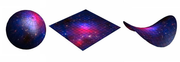
Figure 4: 2-dimensional examples of positive, zero and negative curvature universes (from left to right respectively). The zero and negative ones show only a finite part of the space, which extend to infinity in all directions.

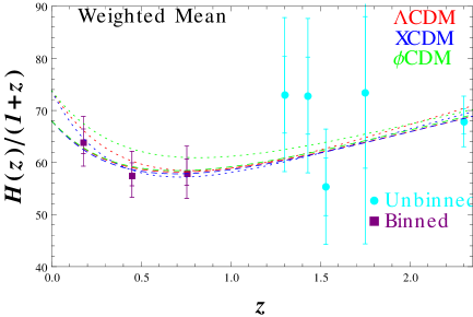
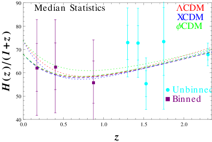
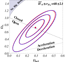
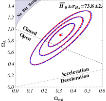
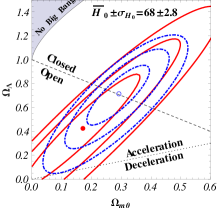
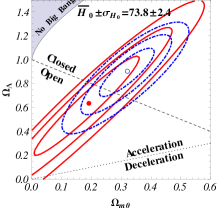
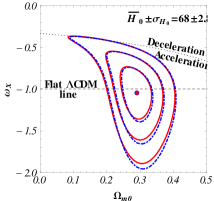
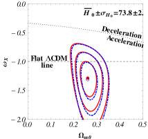
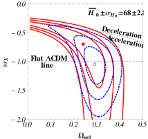
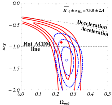
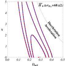
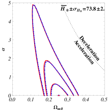
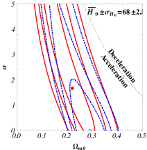
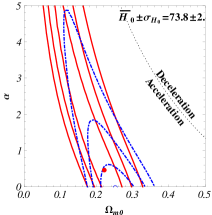
Figure 4: Top left (right) panel shows the $H(z)/(1+z)$ data, binned with 7 or 9 measurements per bin, as well as 5 higher $z$ measurements, and the Farooq & Ratra⁶² best-fit model predictions, dashed (dotted) for lower (higher) $H_{0}$ prior. The 2nd through 4th rows show the $H(z)$ constraints for $\Lambda$CDM, XCDM, and $\phi$CDM. Red (blue dot-dashed) contours are 1$\sigma$, 2$\sigma$, and 3$\sigma$ confidence interval results from 7 or 9 measurements per bin (unbinned Farooq & Ratra,⁶² Table 1) data. In these three rows, the first two plots include red weighted-mean constraints while the second two include red median statistics ones. The filled red (empty blue) circle is the corresponding best-fit point. Dashed diagonal lines show spatially-flat models, and dotted lines indicate zero-acceleration models. For quantitative details see Table (4).

These three possibilities are illustrated in Fig. (4). Constant negative curvature surfaces cannot be embedded in 3-D Euclidean space. The saddle-like open surface only approximates constant negative curvature near its center. In each case the corresponding space has neither a special point nor a special direction. Thus, these are 2-dimensional spaces with underlying metrics consistent with the cosmological principle.

Let us examine the 2-sphere as a representative example: We can think of 2-spheres in terms of a 2-dimensional surface embedded in a 3-dimensional space. The center of the sphere is not the part of the space: it is inside the surface. Since a metric defines intrinsic properties of a space that should be independent of any additional embedding dimensions, thus technically it should be possible to express the metric of the 2-sphere in terms of only two coordinates. Now in terms of coordinates $\vec{x}=(x_{1},x_{2},x_{3})$ in the embedding 3-dimensional flat euclidean space, the surface of sphere of radius $D$ is the collection of points that satisfies

$$(x^{1})^{2}+(x^{2})^{2}+(x^{3})^{2}=D^{2},$$ (160)

so differentiating and simplifying we get

$$\Rightarrow(dx^{3})^{2}=\frac{(x^{1}dx^{1}+x^{2}dx^{2})^{2}}{D^{2}-(x^{1})^{2}-(x^{2})^{2}}.$$ (161)

The line elements for the distance between two points $(\vec{x},\vec{x}+d\vec{x})$ on the 2-sphere is

$$dl^{2} = (dx^{1})^{2}+(dx^{2})^{2}+(dx^{3})^{2}.$$ (162)

Using this relation and Eq. (161) we may rewrite this as

$$dl^{2} = (dx^{1})^{2}+(dx^{2})^{2}+\frac{(x^{1}dx^{1}+x^{2}dx^{2})^{2}}{D^{2}-(x^{1})^{2}-(x^{2})^{2}}.$$ (163)

This line element describes distances on the 2-dimensional surface of the sphere and depends on only two coordinates ($D$ is a constant). Distances are specified entirely by coordinates intrinsic to the 2D surface, independent of third embedding dimension. Let us now generalize this discussion to the 3-dimensional homogeneous space.

2 Homogeneous, 3-Dimensional Spaces

Consider a 3-dimensional sphere embedded in a 4-dimensional Euclidean hyperspace

$$\left(x^{1}\right)^{2}+\left(x^{2}\right)^{2}+\left(x^{3}\right)^{2}+\left(x^{4}\right)^{2}=R^{2},$$ (164)

where $R$ is the radius of the 3-dimensional sphere. The distance between two neighboring points in the 4-dimensional space is given by

$$\left(dx^{1}\right)^{2}+\left(dx^{2}\right)^{2}+\left(dx^{3}\right)^{2}+\left(dx^{4}\right)^{2}=dl^{2}.$$ (165)

Differentiating Eq. (164) and solving for $dx^{4}$ , we obtain

$$x^{4}dx^{4} = =-x^{1}dx^{1}-x^{2}dx^{2}-x^{3}dx^{3},$$

$$dx^{4} = -\frac{x^{i}dx^{i}}{\sqrt{R^{2}-x^{i}x^{i}}}.\hskip 28.45274pt\left(\mathrm{recall}\ i\in\left\{1,2,3\right\}\right)$$ (166)

Then Eq. (165) can be rewritten as

$$dl^{2}=\left(dx^{1}\right)^{2}+\left(dx^{2}\right)^{2}+\left(dx^{3}\right)^{2}+\frac{\left(x^{i}dx^{i}\right)^{2}}{R^{2}-x^{i}x^{i}}.$$ (167)

In spherical coordinates

$$x^{1} = r\ \mathrm{sin}\theta\ \mathrm{cos}\phi,$$

$$x^{2} = r\ \mathrm{sin}\theta\ \mathrm{sin}\phi,$$ (168)

$$x^{3} = r\ \mathrm{cos}\theta.$$

Using Eq. (2), and very simple algebra and differential calculus, we find

$$x^{i}x^{i} = \left(dx^{1}\right)^{2}+\left(dx^{2}\right)^{2}+\left(dx^{3}\right)^{2}=r^{2},$$

$$x^{i}dx^{i} = rdr,$$ (169)

$$dx^{i}dx^{i} = dr^{2}+r^{2}d\theta^{2}+\left(r\ \mathrm{sin}\theta\right)^{2}d\phi^{2}.$$

Substituting Eqs. (2) in Eq. (167), we can express the differential length element $dl^{2}$ in terms of polar coordinates and $R$ as

$$dl^{2} = \frac{dr^{2}}{1-\left(\frac{r}{R}\right)^{2}}+r^{2}d\theta^{2}+\left(r\ \mathrm{sin}\theta\right)^{2}d\phi^{2}.$$ (170)

The 3-sphere (with $R^{2}>0$) has the following important properties:

1. It corresponds to a homogeneous, isotropic space that is closed and bounded.

2. It has great circles as geodesics.

3. It is a space of constant positive curvature.

4. An ant dropped onto the surface of an otherwise featureless 3-sphere would find that:

   1. No point or direction appears any different from any other.

   2. The shortest distance between any two points corresponds to a segment of a great circle.

   3. A sufficiently long journey in a fixed direction would return one to the starting point.

   4. The total area of the sphere was finite.

We can also have a negatively curved 3-dimensional space (a “saddle”) where in the above we have to replace $R^{2}$ with $-R^{2}$. Then

$$\left(x^{1}\right)^{2}+\left(x^{2}\right)^{2}+\left(x^{3}\right)^{2}+\left(x^{4}\right)^{2}=-R^{2},$$

$$\Rightarrow\ \ \ dl^{2}=\frac{dr^{2}}{1+\left(\frac{r}{R}\right)^{2}}+r^{2}d\theta^{2}+\left(r\ \mathrm{sin}\theta\right)^{2}d\phi^{2}.$$ (171)

This negatively curved 3-dimensional space have the following important properties:

1. It is a homogeneous and isotropic, space that is unbounded and infinite.

2. It has hyperbolas as geodesics.

3. It is a space of constant negative curvature.

4. An ant dropped onto the this surface would find that:

   1. No point or direction appears any different from any other.

   2. The shortest distance between any two points corresponds to a segment of a hyperbola.

   3. The ant would never return to the starting point by continuing an infinite distance in a fixed direction.

   4. The ant would find that the volume of the space is infinite.

Finally the 3-dimensional flat Euclidean case is the $R\rightarrow\infty$ limit of either of the above space. It has

$$dl^{2}=dr^{2}+r^{2}d\Omega^{2}=dr^{2}+r^{2}d\theta^{2}+r^{2}\mathrm{sin^{2}}\theta d\phi^{2}.$$ (172)

This space has the following properties:

1. It is homogeneous and isotropic.

2. It is of infinite extent, with straight lines as geodesics.

3. Obviously, this space corresponds to the limit of zero spatial curvature.

4. The volume of this space is infinite, and a straight path in one direction will never return to the starting point.

In summary, $dl^{2}$ is given by

$$dl^{2} = \frac{dr^{2}}{1-k\ r^{2}}+r^{2}d\theta^{2}+\left(r\ \mathrm{sin}\theta\right)^{2}d\phi^{2},$$ (173)

where $k=1/R^{2}$ can be positive, zero, negative and the corresponding spacetime interval is

$$ds^{2} = -dt^{2}+\frac{dr^{2}}{1-k\ r^{2}}+r^{2}d\theta^{2}+\left(r\ \mathrm{sin}\theta\right)^{2}d\phi^{2}.$$ (174)

Where $k$ negative, zero, and positive correspond to an infinitely open or negatively curved Universe, an infinitely flat Universe and a finite closed Universe respectively.

The metric in Eq. (174) is the metric of stationary curved spacetime. As a special case we can put $k=0$, and we will recover the Minkowski flat spacetime metric, which applies only within the context of special relativity, so called, because it deals with the special case in which spacetime is not curved by the presence of mass and energy. Without any gravitational effects, Minkowski spacetime is flat and static. Using Eq. (10), we can write the above metric as:

$$ds^{2} = -dt^{2}+\frac{dr^{2}}{1-k\ r^{2}}+r^{2}d\Omega^{2}.$$ (175)

When gravity is added, however, the permissible spacetimes are more interesting. With the assumption of homogeneity of space, the spatial components of the metric tensor can still be time dependent. The generic line element which meets these conditions is:

$$ds^{2} = -dt^{2}+a^{2}(t)\left[\frac{dr^{2}}{1-k\ r^{2}}+r^{2}d\Omega^{2}\right].$$ (176)

The term in square bracket in above equation is the spatial part of the metric that does not depend on time; all the time dependence is in the function $a^{2}(t)$, where $a(t)$ is the scale factor. Note that the substitutions

$$k\rightarrow\frac{k}{|k|},$$

$$r\rightarrow\sqrt{|k|}r,$$ (177)

$$a\rightarrow\frac{a}{\sqrt{|k|}},$$

leaves Eq. (176) invariant. Therefore, the only relevant parameter is $k/|k|$, which can have only three discrete values: $-1,\ 0,\ \mathrm{and}\ 1$, corresponding to the hyperbolic, flat, and spherical Universe respectively. Also $t$ is the comoving cosmic time and $d\Omega^{2}$ is the line element of the unit 2-sphere. Here it is important to note that locally we actually see around us the distribution of matter in the form of stars, galaxies, galaxy clusters and so on. The local spacetime structure around such objects is certainly different from what is given by the above line element. This above line element is meant to describe the spacetime of cosmology on much large scale, scale of about 100 Mpc and larger, where the cosmological principle is valid.

The above Friedmann-Lemaître-Robertson-Walker (FLRW) spacetime line element may be expressed in an alternative form by introducing the 4-dimensional generalization of polar angles

$$w = R\ \mathrm{cos}\chi,$$ (178)

$$x = R\ \mathrm{sin}\chi\mathrm{sin}\theta\mathrm{cos}\phi,$$ (179)

$$y = R\ \mathrm{sin}\chi\mathrm{sin}\theta\mathrm{sin}\phi,$$ (180)

$$z = R\ \mathrm{sin}\chi\mathrm{cos}\theta,$$ (181)

with the ranges $0\leq\phi\leq 2\pi$, $0\leq\theta\leq\pi$, and $0\leq\chi\leq\pi$ for the case of spherical geometry and with the substitution $w=iw$, $\chi=i\chi$, and $R=iR$ for hyperbolic geometry.

The Friedmann-Lemaître-Robertson-Walker (FLRW) spacetime line element may be written as:

$$ds^{2}=-dt^{2}+a^{2}(t)\left\{\begin{array}[]{lc}d\chi^{2}+\mathrm{sin^{2}}\chi\left(d\theta^{2}+\mathrm{sin^{2}}\theta d\phi^{2}\right)&\ \ \ \ \mathrm{(closed)}\\ d\chi^{2}+\chi^{2}\left(d\theta^{2}+\mathrm{sin^{2}}\theta d\phi^{2}\right)&\ \ \ \ \mathrm{(flat)}\\ d\chi^{2}+\mathrm{sinh^{2}}\chi\left(d\theta^{2}+\mathrm{sin^{2}}\theta d\phi^{2}\right)&\ \ \ \ \mathrm{(open)}\\ \end{array},\right.$$ (185)

which is related to

$$ds^{2} = -dt^{2}+a^{2}(t)\left[\frac{dr^{2}}{1-k\ r^{2}}+r^{2}d\theta^{2}+r^{2}\mathrm{sin^{2}}\theta d\phi^{2}\right].,$$ (186)

by the change of variables:

$$r=\left\{\begin{array}[]{lc}\mathrm{sin}\chi&\ \ \ \ \mathrm{(closed)}\\ \chi&\ \ \ \ \mathrm{(flat)}\\ \mathrm{sinh^{2}}\chi&\ \ \ \ \mathrm{(open)}\\ \end{array}.\right.$$ (190)

Here it is important to take note of the following points:

1. The derivation of the FLRW metric was purely geometrical, subject to the constraints of homogeneity.

2. No dynamical considerations enter explicitly into its formulation.

3. Of course, dynamics are implicit, to the extent that the overall dynamical structure of the Universe must be consistent with the cosmological principle that was used to construct the metric.

The Friedmann-Lemaître-Robertson-Walker (FLRW) the line element may be expressed in matrix form as

$$ds^{2} = g_{\mu\nu}dx^{\mu}dx^{\nu},$$ (200)

$$= \left(\begin{array}[]{cccc}dt&dr&d\theta&d\phi\\ \end{array}\right)\left(\begin{array}[]{cccc}-1&0&0&0\\ 0&\frac{a^{2}(t)}{1-kr^{2}}&0&0\\ 0&0&a^{2}(t)r^{2}&0\\ 0&0&0&r^{2}\mathrm{sin^{2}}\theta\\ \end{array}\right)\left(\begin{array}[]{c}dt\\ dr\\ d\theta\\ d\phi\\ \end{array}\right)$$

Thus, the FLRW metric is diagonal, with non zero covariant elements

$$g_{00}=-1,\hskip 14.22636ptg_{11}=\frac{a^{2}}{1-kr^{2}},\hskip 14.22636ptg_{22}=a^{2}r^{2},\hskip 14.22636ptg_{33}=a^{2}r^{2}\mathrm{sin^{2}}\theta,$$ (201)

and the corresponding contravariant components are

$$g^{00}=-1,\hskip 14.22636ptg^{11}=\frac{1-kr^{2}}{a^{2}},\hskip 14.22636ptg^{22}=\frac{1}{a^{2}r^{2}},\hskip 14.22636ptg^{33}=\frac{1}{a^{2}r^{2}\mathrm{sin^{2}}\theta}.$$ (202)

6 Derivation of Friedmann’s Equations from General Relativity

Though we can derive Friedmann’s equations of motion which are the backbone of cosmology almost entirely by using Newtonian Mechanics (interested readers can see, Liddle,⁹⁷ Ryden,¹⁴⁷ or Raine and Thomas.¹³⁷), here we derive them from Einstein’s general relativity field equations.

Considering the most general Friedmann-Lemaitre-Robertson-Walker (FLWR) metric given in Eq. (176), the only non-zero elements and first derivative of the metric are

$$g_{00} = -1,\hskip 56.9055ptg^{00}=-1,$$

$$g_{11} = \frac{a^{2}}{1-kr^{2}},\hskip 31.29802ptg^{11}=\frac{1-kr^{2}}{a^{2}},$$

$$g_{22} = a^{2}r^{2},\hskip 51.21495ptg^{22}=\frac{1}{a^{2}r^{2}},$$

$$g_{33} = a^{2}r^{2}\mathrm{sin^{2}}\theta,\hskip 25.60747ptg^{33}=\frac{1}{a^{2}r^{2}\mathrm{sin^{2}}\theta},$$

$$g_{11,0} = \frac{2a\dot{a}}{1-kr^{2}},$$

$$g_{11,1} = \frac{2kra^{2}}{(1-kr^{2})^{2}},$$

$$g_{22,0} = 2a\dot{a}\ r^{2},$$

$$g_{22,1} = 2a^{2}r,$$

$$g_{33,0} = 2a\dot{a}r^{2}\ \mathrm{sin^{2}}\theta,$$

$$g_{33,1} = 2a^{2}r\ \mathrm{sin^{2}}\theta,$$

$$g_{33,2} = 2a^{2}r^{2}\mathrm{sin}\theta\ \mathrm{cos}\theta.$$ (203)

We now compute the Christoffel symbols

$$\Gamma^{\gamma}_{\alpha\beta}=\frac{1}{2}g^{\gamma\delta}\Big{(}g_{\delta\alpha,\beta}+g_{\beta\delta,\alpha}-g_{\alpha\beta,\delta}\Big{)}.$$ (204)

Let’s compute term by term:

• Time-Time Terms

  We put $\gamma=0$, hence also have to set $\delta=0$, to ensure $g^{\gamma\delta}$ is non-zero,

  $$\Gamma^{0}_{\alpha\beta}=\frac{1}{2}g^{00}\Big{(}g_{0\alpha,\beta}+g_{\beta 0,\alpha}-g_{\alpha\beta,0}\Big{)}=-\frac{1}{2}g^{00}g_{\alpha\beta,0}=\frac{1}{2}g_{\alpha\beta,0}.$$ (205)

  Here we use Eqs. (203) and the fact that $g_{0\alpha,\beta}=g_{\beta 0,\alpha}=0$. From this we have

  $$\Gamma^{0}_{00} = \Gamma^{0}_{\alpha 0}=\Gamma^{0}_{0\beta}=0,$$ (206)

  $$\Gamma^{0}_{ij} = \frac{1}{2}g_{ij,0}.\hskip 42.67912pt\left(\mathrm{where~{}~{}}i,j\ \in\left\{1,2,3\right\}\right)$$ (207)

  $$\Rightarrow\Gamma^{0}_{12}=\Gamma^{0}_{13}=\Gamma^{0}_{21}=\Gamma^{0}_{23}=\Gamma^{0}_{31}=\Gamma^{0}_{32}=0,$$ (208)

  and the $i=j$ terms are

  $$\Gamma^{0}_{11} = \frac{1}{2}\left(\frac{2a\dot{a}}{1-kr^{2}}\right)=\frac{a\dot{a}}{1-kr^{2}},$$ (209)

  $$\Gamma^{0}_{22} = \frac{1}{2}\left(2a\dot{a}r^{2}\right)=a\dot{a}r^{2},$$ (210)

  $$\Gamma^{0}_{33} = \frac{1}{2}\left(2a\dot{a}r^{2}\mathrm{sin^{2}}\theta\right)=a\dot{a}r^{2}\mathrm{sin^{2}}\theta.$$ (211)

• Space-Time Terms

  Let $\alpha=0$ and $\gamma=i$ in Eq. (204), we will get

  $$\Gamma^{i}_{0\beta}=\frac{1}{2}g^{ij}\big{(}g_{j0,\beta}+g_{\beta j,0}-g_{0\beta,j}\Big{)}.$$ (212)

  The first and third term in the parentheses are zero (because our metric is diagonal), the second term is also zero unless $\beta=j$, in which case:

  $$\Gamma^{i}_{0\beta} = \frac{1}{2}g^{ij}g_{ij,0}\delta^{i}_{\beta},$$ (213)

  $$= \frac{1}{2}g^{ij}\left(\frac{2a\dot{a}}{a^{2}}g_{ij}\right)\delta^{i}_{\beta},\hskip 28.45274pt\left(\because\ g_{ij,0}=\frac{2a\dot{a}}{a^{2}}g_{ij},\ \ \mathrm{from\ Eq.\ (\ref{eq:metricandderivatives})}\right)$$

  $$= \frac{\dot{a}}{a}g^{ij}g_{ij}\delta^{i}_{\beta},$$

  $$= \frac{\dot{a}}{a}\delta^{i}_{\beta}.$$

• Space-Space Terms

  We need to use $\alpha=j,\ \beta=k,\mathrm{and}\ \gamma=i$ in Eq. (204),

  $$\Gamma^{i}_{jk}=\frac{1}{2}g^{il}\Big{(}g_{lj,i}+g_{kl,j}-g_{jk,l}\Big{)},$$ (214)

  then the required Christoffel symbols will be:

  $$\Gamma^{1}_{11} = \frac{1}{2}g^{11}\big{(}g_{11,1}+\cancel{g_{11,1}}-\cancel{g_{11,1}}\big{)}=\frac{1}{2}g^{11}g_{11,1}=\frac{kr}{1-kr^{2}},$$

  $$\Gamma^{1}_{22} = \frac{1}{2}g^{11}\big{(}g_{12,2}+g_{21,2}-g_{22,1}\big{)}=-r(1-kr^{2}),$$

  $$\Gamma^{1}_{33} = \frac{1}{2}g^{11}\big{(}g_{13,3}+g_{31,3}-g_{33,1}\big{)}=-r(1-kr^{2})\mathrm{sin^{2}}\theta,$$

  $$\Gamma^{2}_{33} = \frac{1}{2}g^{22}\big{(}g_{23,3}+g_{32,3}-g_{33,2}\big{)}=-\mathrm{sin}\theta\mathrm{cos}\theta,$$

  $$\Gamma^{2}_{12} = \Gamma^{2}_{21}=\frac{1}{2}g^{22}\big{(}g_{22,1}+g_{12,2}-g_{21,2}\big{)}=\frac{1}{r},$$

  $$\Gamma^{3}_{13} = \Gamma^{3}_{11}=\frac{1}{2}g^{33}\big{(}g_{33,1}+g_{13,3}-g_{31,3}\big{)}=\frac{1}{r},$$

  $$\Gamma^{3}_{23} = \Gamma^{3}_{22}=\frac{1}{2}g^{33}\big{(}g_{33,2}+g_{23,3}-g_{32,3}\big{)}=\mathrm{cot}\theta.$$ (215)

  All other terms are zero.

Now we can compute the Ricci tensor, using Eq. (101),

$$R^{\gamma}_{\alpha\gamma\beta}=R_{\alpha\beta}=\Gamma^{\gamma}_{\alpha\beta,\gamma}-\Gamma^{\gamma}_{\gamma\alpha,\beta}+\Gamma^{\gamma}_{\gamma\lambda}\Gamma^{\lambda}_{\beta\alpha}-\Gamma^{\gamma}_{\beta\lambda}\Gamma^{\lambda}_{\gamma\alpha}.$$ (216)

The $R_{00}$ component is

$$R_{00}=\Gamma^{\gamma}_{00,\gamma}-\Gamma^{\gamma}_{\gamma 0,0}+\Gamma^{\gamma}_{\gamma\lambda}\Gamma^{\lambda}_{00}-\Gamma^{\gamma}_{0\lambda}\Gamma^{\lambda}_{\gamma 0}.$$ (217)

It is very easy to see that the first and the third term are zero because $\Gamma^{\gamma}_{00}=0$ from Eq. (215). Hence we have

$$R_{00}=-\Gamma^{\gamma}_{\gamma 0,0}-\Gamma^{\gamma}_{0\lambda}\Gamma^{\lambda}_{\gamma 0}.$$ (218)

The first term is

$$\Gamma^{\gamma}_{\gamma 0,0} = \frac{d}{dx^{0}}\left[\Gamma^{\gamma}_{\gamma 0}\right],$$ (219)

$$= \frac{d}{dx^{0}}\left(\frac{\dot{a}}{a}\delta^{\gamma}_{\gamma}\right),\hskip 28.45274pt\Big{(}\mathrm{using\ Eq.\ (\ref{eq:FtGRgamma})}\Big{)}$$

$$= \frac{d}{dx^{0}}\left(3\frac{\dot{a}}{a}\right),$$

$$= 3\left(\frac{a\ddot{a}-\dot{a}^{2}}{a^{2}}\right).$$

Now, the second term on the right hand side of Eq. (218) is zero if $\gamma=0$ so

$$\Gamma^{\gamma}_{0\lambda}\Gamma^{\lambda}_{\gamma 0} = \Gamma^{i}_{0j}\Gamma^{j}_{i0}$$ (220)

$$= \left(\frac{\dot{a}}{a}\right)\delta^{i}_{j}\left(\frac{\dot{a}}{a}\right)\delta^{j}_{i},\hskip 28.45274pt\Big{(}\mathrm{using\ Eq.\ (\ref{eq:FtGRgamma})}\Big{)}$$

$$= \left(\frac{\dot{a}}{a}\right)^{2}\underbrace{\delta^{i}_{j}\ \delta^{j}_{i}}_{=3},$$

$$= 3\left(\frac{\dot{a}}{a}\right)^{2}.$$

Now Eq. (218) with Eq. (219) and Eq. (220) results

$$R_{00} = -3\left(\frac{a\ddot{a}-\dot{a}^{2}}{a^{2}}\right)-3\left(\frac{\dot{a}}{a}\right)^{2}=-3\frac{\ddot{a}}{a}.$$ (221)

Hence we can raise an index to get

$$R^{0}_{0}=g^{00}R_{00}=-R_{00}=3\ \frac{\ddot{a}}{a}.$$ (222)

Along the same lines, straightforward, yet tedious, computation yields the other non-zero components of the Ricci tensor,

$$R_{11} = \frac{a\ddot{a}+2\dot{a}^{2}+2k}{1-kr^{2}},$$

$$R_{22} = r^{2}\left(a\ddot{a}+2\dot{a}^{2}+2k\right),$$

$$R_{22} = r^{2}\left(a\ddot{a}+2\dot{a}^{2}+2k\right)\mathrm{sin^{2}}\theta.$$ (223)

These can be written in a compact form after raising the index,

$$R^{0}_{i} = 0,$$

$$R^{i}_{j} = \frac{1}{a^{2}}\left(a\ddot{a}+2\dot{a}^{2}+2k\right)\delta^{i}_{j}.$$ (224)

The Universe is not empty, so we are interested in non-vacuum solutions to Einstein’s equations. We will choose to model the matter and energy in the Universe by perfect fluids. We discussed perfect fluids earlier. They are defined as fluids which are isotropic in their rest frame. The energy-momentum tensor for a perfect fluid can be written as

$$T_{\alpha\beta}=\left(\rho+P\right)u_{\alpha}u_{\beta}+Pg_{\alpha\beta}.$$ (225)

Raising the index of the stress-energy tensor we have

$$T^{\alpha}_{\beta} = \left(\rho+P\right)u^{\alpha}u_{\beta}+P\delta^{\alpha}_{\beta}.$$ (226)

Here $\rho$ and $P$ are the energy density and pressure as measured in the rest frame, and $u^{\nu}$ is the 4-velocity of the fluid. A fluid that is isotropic in some frame must lead to a metric isotropic in that frame. That is, the fluid must be at rest in comoving coordinates. The final 4-velocity is then

$$u^{\nu}=(1,0,0,0),$$ (227)

and lowering the index gives

$$u_{\nu}=(-1,0,0,0).$$ (228)

Now, we shall have need for the contraction over indices $\alpha$ and $\beta$ of Eq. (226),

$$T\equiv T^{\alpha}_{\alpha}=-\left(\rho+P\right)+4P=3P-\rho.$$ (229)

Raising an index of Einstein’s field equations gives

$$R^{\alpha}_{\beta}-\frac{1}{2}\delta^{\alpha}_{\beta}\mathcal{R} = 8\pi GT^{\alpha}_{\beta}.$$ (230)

Contracting over indices $\alpha$ and $\beta$ of Eq. (230) we have

$$-\mathcal{R}=8\pi GT,\hskip 28.45274pt\Big{(}\mathrm{where}\ T\equiv T^{\alpha}_{\alpha},\ \delta^{\alpha}_{\alpha}=4,\ \mathrm{and}\ R^{\alpha}_{\alpha}=\mathcal{R}.\Big{)}$$ (231)

Hence Einstein’s field equation can also be written as

$$R^{\alpha}_{\beta}=8\pi G\left(T^{\alpha}_{\beta}-\frac{1}{2}\delta^{\alpha}_{\beta}T\right).$$ (232)

Using Eq. (226) and Eq. (229) in Eq. (232), we will find

$$R^{\alpha}_{\beta} = 8\pi G\left[\left(\rho+P\right)u^{\alpha}u_{\beta}+P\delta^{\alpha}_{\beta}-\frac{1}{2}\delta^{\alpha}_{\beta}\left(3P-\rho\right)\right],$$ (233)

$$= 8\pi G\left[\left(\rho+P\right)u^{\alpha}u_{\beta}+\frac{1}{2}\delta^{\alpha}_{\beta}\left(\rho-P\right)\right].$$

The $R^{0}_{0}$ component of Eq. (233) is

$$R^{0}_{0} = 8\pi G\left[-\left(\rho+P\right)+\frac{1}{2}\left(\rho-P\right)\right]$$ (234)

$$= 8\pi G\left[-\frac{1}{2}\left(\rho+3P\right)\right]=-4\pi G\left(\rho+3P\right).$$

Comparing this with Eq. (222), leads to standard acceleration equation as:

$$\frac{\ddot{a}}{a}=-\frac{4\pi G}{3}\left(\rho+3P\right).$$ (235)

Similarly, comparing the $R^{i}_{i}$ component of Eq. (233) with Eq. (224), leads to the other standard Friedman equation as follows

$$\frac{1}{a^{2}}\left(a\ddot{a}+2\dot{a}^{2}+2k\right) = 8\pi G\left[0+\frac{1}{2}\left(\rho-P\right)\right],$$

$$\Rightarrow\left(\frac{\ddot{a}}{a}\right)+2\left(\frac{\dot{a}}{a}\right)^{2}+2\frac{k}{a^{2}} = 4\pi G(\rho-P),$$

$$\Rightarrow\left(\frac{\dot{a}}{a}\right)^{2} = \frac{8\pi G}{3}\rho-\frac{k}{a^{2}}.$$ (236)

Here we have used Eq. (235) in the last step. By combining this with the conservation of energy equation, that we already derived in Sec. (3), and the equation of state, we obtain a closed system of Friedmann equations.

7 Solutions of Friedmann’s Equations

Given the closed set of cosmological equations of motion, which gives the relationship between the scale factor $a(t)$, the energy density $\rho(t)$ ($c=1$, mass and energy have the same units), and pressure $P$, for open, flat and closed Universe models (as denoted by three discrete values of $k=-1,\ 0,$ and, $1$ respectively), we can solve these equations in various cases and obtain the form of the scale factor $a(t)$ as a function of time. Let’s start with the definition of the deceleration parameter.

1 Deceleration Parameter

From the definition of Hubble parameter $H$ in Eq. (157) we have

$$\dot{H} = \frac{a\ddot{a}-\dot{a}^{2}}{a^{2}}=-H^{2}+\frac{\ddot{a}}{a}=-H^{2}\left(1-\frac{\ddot{a}}{H^{2}a}\right)\equiv-H^{2}(1+q),$$ (237)

where the dimensionless deceleration parameter $q$ is defined as

$$q\equiv-\frac{\ddot{a}}{H^{2}a}.$$ (238)

The present value of all time-dependent quantities are denoted by a subscript of $0$ for example, the present value of the deceleration parameter is denoted by $q_{0}$ and is

$$q_{0}=-\frac{1}{H_{0}^{2}}\left(\frac{\ddot{a}}{a}\right)_{0}.$$ (239)

Note the choice of sign in defining $q_{0}$. Since $H_{0}^{2}$ and $a$ are strictly positive numbers, $q_{0}<0$ for $\ddot{a}>0$ and vice-versa, which means a negative value of $q_{0}$ represents an accelerating cosmological expansion.

2 Curvature-Dominated Universe ($k\neq 0$, $q_{0}=0$, $\rho_{i}=0$)

The simplest (but not interesting) Universe is one that is completely empty, no matter, no energy, no radiation, etc. For such Universe, the Friedmann equation takes the form

$$\dot{a}^{2}=-k.$$ (240)

This equation has two solutions. The first is $\dot{a}=0$ and $k=0$ has the solutions $a=$ constant which is the spatially-flat static Minkowski spacetime. The second one is governed by

$$\dot{a}=\pm\sqrt{-k},$$ (241)

which is physically consistent only when $k=-1$ (since $\dot{a}$ cannot be complex). A Universe that is positively curved and empty is not allowed by Friedmann’s equations. In the negative curvature case, solving the differential equation Eq. (241), gives:

$$a(t)\propto t.$$ (242)

This is negative space-curvature Milne spacetime. In the language of Newtonian mechanics, in the absence of any gravitational force (as in this case) the relative velocity of any two points in space is constant, which leads to the scale factor $a(t)$ being a linear function of time in an empty Universe. From the second Friedmann equation, we get

$$\hskip 56.9055pt\frac{\ddot{a}}{a}=0.\hskip 28.45274pt(\mathrm{since}\ \rho=p=\Lambda=0)$$ (243)

This means that an empty Universe, which has to be negatively curved, should expand with zero acceleration. Also from Eq. (238) we see:

$$-H^{2}q=0,$$ (244)

since $H\neq 0$ this implies that $q=0$.

Note that in an empty Universe since $H=\dot{a}/a=t^{-1}$, $t_{0}$, the age of the Universe is equal to the Hubble time,

$$t_{0}=H_{0}^{-1},$$ (245)

because there is nothing to speed up or slow down expansion.

3 Spatially-Flat Single-Component Universe (${k=0,\ q_{0}=(1+3\omega)/2}$)

In a spatially-flat Universe, $k=0$, the Friedmann equation is

$$\left(\frac{\dot{a}}{a}\right)^{2}=\frac{8\pi G}{3}\rho,$$ (246)

where $\rho$ is the time dependent energy density of the single type of matter present in Universe. From the energy evolution equation [see Eq. (142) with the general assumption of $a_{0}=1$];

$$\rho(t)=\rho_{0}a^{-3(1+\omega)},$$ (247)

where $a(t)$ is the scale factor, and we have assumed an ideal fluid of time independent equation of state parameter $\omega$. Hence, Eq. (246) takes the form

$$\left(\frac{\dot{a}}{a}\right)^{2}=\frac{8\pi G}{3}\rho_{0}a^{-3(1+\omega)}.$$ (248)

To find how the scale factor $a(t)$ evolves in this kind of Universe, we have to solve the above differential equation. In order to do that, let’s guess a power law solution $a\propto t^{p}$, then the left and right hand side of Eq. (248) evolve with time as

$$\hskip 85.35826pt\left(\frac{\dot{a}}{a}\right)^{2}\propto t^{-2},\hskip 14.22636pt\frac{8\pi G}{3}\rho_{0}a^{-3(1+\omega)}\propto t^{-3p(1+\omega)}.$$ (249)

Matching the powers of $t$ we get

$$p = \frac{2}{3(1+\omega)},$$ (250)

with the restriction of $\omega\neq-1$. Hence:

$$a(t)\propto t^{2/3(1+\omega)}.$$ (251)

If $\omega\neq-1/3$, $\ddot{a}\neq 0$ and this particular Universe is undergoing accelerated or decelerated expansion. From the second Friedmann’s equation

$$\frac{\ddot{a}}{a}=-\frac{4\pi G}{3}\rho\left(1+3\omega\right).$$ (252)

In terms of deceleration parameter, $\ddot{a}/a=-qH^{2}$, this equation gives

$$\rho = \frac{3H^{2}}{4\pi G(1+3\omega)}q,$$ (253)

which when substituted in the first Friedmann equation $H^{2}=8\pi G\rho/3$, gives

$$H^{2}\left(1-\frac{2}{1+3\omega}q\right) = 0.$$ (254)

Since $H\neq 0$,

$$q=\frac{1}{2}\left(1+3\omega\right).$$ (255)

Hence $q$ of the spatially-flat Universe is $\left(1+3\omega\right)/2$.

We now define the critical density of the Universe, which is the density of the matter when $q=1/2$ (spatially-flat case) with $\omega=0$ or pressure less matter. From Eq. (253),

$$\rho_{cr}=\frac{3H^{2}}{8\pi G}.$$ (257)

This is the density needed to yield a spatially-flat Universe. Numerically this is

$$\rho_{cr}=1.88\times 10^{-29}\ h^{2}\mathrm{g~{}cm^{-3}},$$ (258)

The deceleration parameter $q$ relates the density of the Universe $\rho$ to the critical density $\rho_{cr}$ through

$$q=\frac{\rho}{2\rho_{cr}}\left(1+3\omega\right).$$ (259)

From Eq. (251) $H={2}/({3(1+\omega)t})$, so the age of the Universe, $t_{0}$, in terms of the Hubble constant, is

$$t_{0}=\frac{2}{3(1+\omega)}H^{-1}_{0}.$$ (260)

If $\omega<-1/3$ then the age of the single-component-dominated spatially-flat Universe is larger than the Hubble time $1/H_{0}$, and if $\omega>-1/3$ the age is less than the Hubble time.

Now let’s consider two special cases of the spatially-flat Universe.

• Non-Relativistic-Matter-Dominated Universe ($\boldsymbol{k=0,\ P=0}$)

  Non-Relativistic matter (dust) does not exert pressure, hence $P=0$ and also $\omega=0$. From Eqs. (142) and (251) we get

  $$\rho_{m}(t)=\rho_{m0}a^{-3}(t),$$ (261)

  and integrating Friedmann differential equation we find

  $$a(t)=(6\pi G\rho_{m0}a^{3}_{0})^{1/3}t^{2/3},$$ (262)

  where constant of integration has been chosen so that, $a(t=0)=0$. This Universe is called Einstein-de Sitter spacetime or model.

  Since $\rho_{m}a^{3}=$ constant we can put $\rho_{m}a^{3}=\rho_{m0}a^{3}_{0}$ in Eq. (262) to obtain

  $$\rho_{m}(t)=\frac{1}{6\pi Gt^{2}},$$ (263)

  for the density as a function of time. The age of the Universe can be computed from Eq. (260) as

  $$t_{0}=\frac{2}{3H_{0}}.$$ (264)

  Also, the deceleration parameter for Einstein-de Sitter Universe is

  $$q=\frac{1}{2}.$$ (265)

• Relativistic-Matter-Dominated Universe ($k=0$, $P=\rho/3$)

  Radiation is often modeled by the perfect fluid approximation with $P=\rho/3$ or $\omega=1/3$. Using this value of $\omega$ in Eqs. (142) and (251), we will

  $$\rho_{r}(t)=\rho_{r0}a^{-4}(t),$$ (266)

  and integrating the Friedmann equation we find

  $$a(t)=\left(\frac{32\pi G}{3}\rho_{r0}a^{4}_{0}\right)^{1/4}t^{1/2},$$ (267)

  where the constant of integration has been chosen so that, $a(t=0)=0$.

  Since $\rho_{r}a^{4}=$constant we can put $\rho_{r}a^{4}=\rho_{r0}a^{4}_{0}$ in Eq. (267) to obtain

  $$\rho_{r}(t)=\frac{3}{32\pi Gt^{2}},$$ (268)

  for the density as a function of time. The age of the Universe can be computed from Eq. (260) as

  $$t_{0}=\frac{1}{2H_{0}}.$$ (269)

  Also, the deceleration parameter for the spatially-flat relativistic-matter-dominated Universe is

  $$q=1.$$ (270)

4 Multi-Component Universes

Now let’s consider different cases when the Universe is dominated by two energy density sources at a time. Our basic equations are Friedmann’s equations, so we start with the general form of Friedmann’s equations,

$$\left(\frac{\dot{a}}{a}\right)^{2}=\frac{8\pi G}{3}\sum_{i}\rho_{i}-\frac{k}{a^{2}},$$ (271)

$$\frac{\ddot{a}}{a}=-\frac{4\pi G}{3}\sum_{i}\left(\rho_{i}+3P_{i}\right).$$ (272)

Here $\rho_{i}$ is the time-dependent matter (energy) density contribution of the $i^{th}$ component, and $P_{i}$ is the corresponding pressure exerted by that particular component. The equations of state are:

$$P_{i}=P_{i}(\rho_{i})=\omega_{i}\rho_{i},$$ (273)

where $\omega_{i}$ is dimensionless equation-of-state-parameter of the $i^{th}$ component of matter.

We know our Universe contains matter for which $\rho_{m}\propto a^{-3}$, and radiation for which $\rho_{r}\propto a^{-4}$. Current evidence supports the presence of a cosmological constant with mass density $\rho_{\Lambda}=\rho_{\Lambda 0}=\$constant. It is certainly possible that the Universe contains other components as well, but we will consider only the above-mentioned one. The relative density parameter for the $i^{th}$ component of the Universe is:

$$\Omega_{i}\equiv\frac{\rho_{i}}{\rho_{cr}},\hskip 28.45274pt\rho_{cr}\equiv\frac{3H^{2}}{8\pi G}.$$ (274)

The present values of the density parameter of $i^{th}$ component of Universe is:

$$\Omega_{i0}\equiv\frac{\rho_{i0}}{\rho_{cr}},\ \ \ \ ~{}~{}~{}~{}~{}~{}\mathrm{so}\ \ \ \ ~{}~{}~{}~{}~{}~{}~{}\sum_{i}\Omega_{i0}=1.$$ (275)

Now to be more specific let’s say that $\Omega_{m0}$, $\Omega_{r0}$, $\Omega_{k0}$, and $\Omega_{\Lambda 0}$ are non-relativistic, relativistic, curvature, and cosmological constant density parameters at present time, respectively, then

$$\Omega_{m0}+\Omega_{r0}+\Omega_{k0}+\Omega_{\Lambda 0}=1,$$ (276)

where

$$\Omega_{m0}=\frac{8\pi G}{3H_{0}^{2}}\rho_{m0},\ \ \Omega_{r0}=\frac{8\pi G}{3H_{0}^{2}}\rho_{r0},\ \ \Omega_{k0}=\frac{-k}{(H_{0}a_{0})^{2}},\ \ \Omega_{\Lambda 0}=\frac{\Lambda}{3H_{0}^{2}}.$$ (277)

Hence, the Friedmann’s equation takes the form:

$$\left(\frac{\dot{a}}{a}\right)^{2} = H^{2}_{0}\left[\Omega_{r0}a^{-4}+\Omega_{m0}a^{-3}+\Omega_{\Lambda 0}+\Omega_{k0}a^{-2}\right],$$ (278)

$$= H^{2}_{0}\left[\Omega_{r0}a^{-4}+\Omega_{m0}a^{-3}+\Omega_{\Lambda 0}+(1-\Omega_{0})a^{-2}\right].$$

Here

$$\Omega_{0}=\Omega_{r0}+\Omega_{m0}+\Omega_{\Lambda 0},$$ (279)

will determine the value of this source curvature. If $\Omega_{0}<1$ then $k=-1$, if $\Omega_{0}=1$ then $k=0$, and if $\Omega_{0}>1$ then $k=+1$. Recent analyses of the observable data indicates that the space-curvature term $\frac{1-\Omega_{0}}{a^{2}}$ is probably small but not necessarily zero but very small.^{90, 59}

Let’s consider the two special cases, the non-flat Universe dominated by non relativistic matter, and the non-flat Universe dominated by relativistic matter and compute the scale factor $a(t)$. We will see that, it is not possible to get the scale factor $a(t)$ as an explicit function of time $t$, and, we will instead derive parametric solutions.

• Curvature and Non-Relativistic-Matter-Dominated Universe (${k\neq 0}$, ${P=0}$, ${q_{0}\neq 1/2}$)

  In this case (when $\Omega_{r0}=0$ and $\Omega_{\Lambda 0}=0\ \mathrm{so}\ \Omega_{m0}=\Omega_{0}$) the Friedmann equation. (278) takes the form:

  $$\left(\frac{\dot{a}}{a}\right)^{2}=H^{2}_{0}\left[\frac{\Omega_{0}}{a^{3}}+\frac{1-\Omega_{0}}{a^{2}}\right],$$ (280)

  $$\Rightarrow\frac{da}{dt} = H_{0}\left[\frac{\Omega_{0}}{a}+(1-\Omega_{0})\right]^{1/2},$$

  $$\Rightarrow H_{0}t = \int\limits_{0}^{a}\frac{da^{\prime}}{\left[\frac{\Omega_{0}}{a^{\prime}}+(1-\Omega_{0})\right]^{1/2}}.$$ (281)

  There are two cases:

  Case 1. Open Universe (${\Omega_{0}<1}$) with ${k=-1}$, ${q_{0}<1/2}$

  With the substitution,

  $$a^{\prime}(\eta)=\frac{\Omega_{0}}{2\left(1-\Omega_{0}\right)}\left(\mathrm{cosh}\eta-1\right),\ \ \ \ \ \ \ \mathrm{d}a^{\prime}(\eta)=\frac{\Omega_{0}}{2\left(1-\Omega_{0}\right)}\mathrm{sinh}\eta\ \mathrm{d}\eta,$$ (282)

  the indefinite integral in Eq. (281)becomes

  $$H_{0}t = \frac{\Omega_{0}}{2\left(1-\Omega_{0}\right)^{3/2}}\int\frac{\mathrm{sinh}\eta}{\left[\frac{2}{\mathrm{cosh}\eta-1}+1\right]^{1/2}}\ \mathrm{d}\eta,$$ (283)

  $$= \frac{\Omega_{0}}{2\left(1-\Omega_{0}\right)^{3/2}}\int\frac{\displaystyle\sqrt{\mathrm{cosh}\eta-1}\ \mathrm{sinh}\eta}{\displaystyle\sqrt{\mathrm{cosh}\eta+1}}\ \mathrm{d}\eta,$$

  $$= \frac{\Omega_{0}}{2\left(1-\Omega_{0}\right)^{3/2}}\int\left(\mathrm{cosh}\eta-1\right)\ \mathrm{d}\eta,\hskip 19.91692pt\left(\because\mathrm{sinh}\eta=\displaystyle\sqrt{\left(\mathrm{cosh}\eta-1\right)\left(\mathrm{cosh}\eta+1\right)}\right)$$

  $$= \frac{\Omega_{0}}{2\left(1-\Omega_{0}\right)^{3/2}}\left(\mathrm{sinh}\eta-\eta\right)+c_{1}.$$

  Here $c_{1}$ is constant of integration. Using the initial condition $a(t=0)=0$ leads $c_{1}=0$. Hence, the parametric dependence of the scale factor $a(t)$ on time in this Universe is

  $$a(\eta) = \frac{\Omega_{0}}{2\left(1-\Omega_{0}\right)}\left(\mathrm{cosh}\eta-1\right),$$ (284)

  $$t(\eta) = \frac{\Omega_{0}}{2H_{0}\left(1-\Omega_{0}\right)^{3/2}}\left(\mathrm{sinh}\eta-\eta\right).$$ (285)

  In terms of the deceleration parameter $q_{0}$, using Eq. (259) (which can be read as $q_{0}=\Omega_{0}/2$), these lead to:

  $$a(\eta) = \frac{q_{0}}{\left(1-2q_{0}\right)}\left(\mathrm{cosh}\eta-1\right),$$ (286)

  $$t(\eta) = \frac{q_{0}}{H_{0}\left(1-2q_{0}\right)^{3/2}}\left(\mathrm{sinh}\eta-\eta\right).$$ (287)

  Case 2. Closed Universe (${\Omega_{0}>1}$) with ${k=1}$, ${q_{0}>1/2}$

  With the substitution,

  $$a^{\prime}(\theta)=\frac{\Omega_{0}}{2\left(\Omega_{0}-1\right)}\left(1-\mathrm{cos}\theta\right),\ \ \ \ \ \ \ \mathrm{d}a^{\prime}(\theta)=\frac{\Omega_{0}}{2\left(\Omega_{0}-1\right)}\mathrm{sin}\theta\ \mathrm{d}\theta$$ (288)

  the indefinite integral in Eq. (281) becomes

  $$H_{0}t = \frac{\Omega_{0}}{2\left(\Omega_{0}-1\right)^{3/2}}\int\frac{\mathrm{sin}\theta}{\left[\frac{2}{1-\mathrm{cos}\theta}-1\right]^{1/2}}\ \mathrm{d}\theta,$$ (289)

  $$= \frac{\Omega_{0}}{2\left(\Omega_{0}-1\right)^{3/2}}\int\frac{\displaystyle\sqrt{1-\mathrm{cos}\theta}\ \mathrm{sin}\theta}{\displaystyle\sqrt{1+\mathrm{cos}\theta}}\ \mathrm{d}\theta,$$

  $$= \frac{\Omega_{0}}{2\left(\Omega_{0}-1\right)^{3/2}}\int\left(1-\mathrm{cos}\theta\right)\ \mathrm{d}\theta,\hskip 19.91692pt\left(\because\mathrm{sin}\theta=\displaystyle\sqrt{\left(1-\mathrm{cos}\theta\right)\left(1+\mathrm{cos}\theta\right)}\right)$$

  $$= \frac{\Omega_{0}}{2\left(\Omega_{0}-1\right)^{3/2}}\left(\theta-\mathrm{sin}\theta\right)+c_{2}.$$

  Here $c_{2}$ is constant of integration. Using the initial condition $a(t=0)=0$ leads $c_{2}=0$. Hence, the parametric dependence of the scale factor $a(t)$ on time in this Universe is

  $$a(\theta) = \frac{\Omega_{0}}{2\left(\Omega_{0}-1\right)}\left(1-\mathrm{cos}\theta\right),$$ (290)

  $$t(\theta) = \frac{\Omega_{0}}{2H_{0}\left(\Omega_{0}-1\right)^{3/2}}\left(\theta-\mathrm{sin}\theta\right).$$ (291)

  In terms of the deceleration parameter $q_{0}$, we have

  $$a(\theta) = \frac{q_{0}}{\left(2q_{0}-1\right)}\left(1-\mathrm{cos}\theta\right),$$ (292)

  $$t(\theta) = \frac{q_{0}}{H_{0}\left(2q_{0}-1\right)^{3/2}}\left(\theta-\mathrm{sin}\theta\right).$$ (293)

• Curvature and Relativistic-Matter-Dominated Universe (${k\neq 0}$, ${P=\rho/3}$, ${q_{0}\neq 1}$)

  In this case (when $\Omega_{m0}=0$ and $\Omega_{\Lambda 0}=0\ \mathrm{so}\ \Omega_{r0}=\Omega_{0}$) the Friedmann Eq. (271) takes the form:

  $$\left(\frac{\dot{a}}{a}\right)^{2}=H^{2}_{0}\left[\frac{\Omega_{0}}{a^{4}}+\frac{1-\Omega_{0}}{a^{2}}\right],$$ (294)

  $$\Rightarrow\frac{da}{dt} = H_{0}\left[\frac{\Omega_{0}}{a^{2}}+(1-\Omega_{0})\right]^{1/2},$$

  $$\Rightarrow H_{0}t = \int\limits_{0}^{a}\frac{da^{\prime}}{\left[\frac{\Omega_{0}}{a^{\prime 2}}+(1-\Omega_{0})\right]^{1/2}}.$$ (295)

  There are two cases:

  Case 1. Open Universe ($\Omega_{0}<1$) with ${k=-1}$, ${q_{0}<1}$

  With the substitution,

  $$a^{\prime}(\eta)=\sqrt{\frac{\Omega_{0}}{1-\Omega_{0}}}\ \mathrm{sinh}\eta,\ \ \ \ \ \ \ \ \mathrm{d}a^{\prime}(\eta)=\sqrt{\frac{\Omega_{0}}{1-\Omega_{0}}}\ \mathrm{cosh}\eta\ \mathrm{d}\eta,$$ (296)

  the indefinite integral in Eq. (295) becomes

  $$H_{0}t = \frac{\sqrt{\Omega}_{0}}{1-\Omega_{0}}\int\frac{\mathrm{cosh}\eta}{\left[\frac{1}{\mathrm{sinh^{2}}\eta}+1\right]^{1/2}}\ \mathrm{d}\eta,$$

  $$= \frac{\sqrt{\Omega}_{0}}{1-\Omega_{0}}\mathrm{cosh}\eta+c_{3},$$ (297)

  where $c_{3}$ is constant of integration. Using the initial condition $a(t=0)=0$ leads $c_{3}=-\frac{\sqrt{\Omega_{0}}}{1-\Omega_{0}}$. Hence, the parametric dependence of the scale factor $a(t)$ on time in this Universe is

  $$a(\eta) = \sqrt{\frac{\Omega_{0}}{1-\Omega_{0}}}\ \mathrm{sinh}\eta$$ (298)

  $$t(\eta) = \frac{\sqrt{\Omega_{0}}}{H_{0}\left(1-\Omega_{0}\right)}\left(\mathrm{cosh}\eta-1\right).$$ (299)

  In terms of the deceleration parameter $q_{0}$, using Eq. (259) (which can be read as $q_{0}=\Omega_{r0}=\Omega_{0}$), these lead to

  $$a(\eta) = \sqrt{\frac{q_{0}}{1-q_{0}}}\left(\mathrm{sinh}\eta\right),$$ (300)

  $$t(\eta) = \frac{\sqrt{q_{0}}}{H_{0}\left(1-q_{0}\right)}\left(\mathrm{cosh}\eta-1\right).$$ (301)

  
  

  Case 2: Closed Universe (${\Omega_{0}>1}$) with ${k=1}$, ${q_{0}>1}$ :-

  With the substitution,

  $$a^{\prime}(\theta)=\sqrt{\frac{\Omega_{0}}{\Omega_{0}-1}}\ \mathrm{sin}\theta,\ \ \ \ \ \ \ \mathrm{d}a^{\prime}(\theta)=\sqrt{\frac{\Omega_{0}}{\Omega_{0}-1}}\ \mathrm{cos}\theta\ \mathrm{d}\theta.$$ (302)

  the indefinite integral in Eq. (281) becomes

  $$H_{0}t = \frac{\sqrt{\Omega}_{0}}{\Omega_{0}-1}\int\frac{\mathrm{cos}\theta}{\left[\frac{1}{\mathrm{sin^{2}}\theta}+1\right]^{1/2}}\ \mathrm{d}\theta,$$

  (303)

  $$= -\frac{\sqrt{\Omega}_{0}}{\left(\Omega_{0}-1\right)}\mathrm{cos}\theta+c_{4},$$ (304)

  where $c_{4}$ is constant of integration. Using the initial condition $a(t=0)=0$ leads to $c_{4}=\frac{\sqrt{\Omega_{0}}}{\Omega_{0}-1}$. Hence, the parametric dependence of the scale factor $a(t)$ on time in this Universe is

  $$a(\theta) = \sqrt{\frac{\Omega_{0}}{\Omega_{0}-1}}\ \mathrm{sin}\theta,$$ (305)

  $$t(\theta) = \frac{\sqrt{\Omega}_{0}}{H_{0}\left(\Omega_{0}-1\right)}\left(1-\mathrm{cos}\theta\right).$$ (306)

  In terms of the deceleration parameter $q_{0}$, we have

  $$a(\theta) = \sqrt{\frac{q_{0}}{q_{0}-1}}\ \mathrm{sin}\theta,$$ (307)

  $$t(\theta) = \frac{\sqrt{q_{0}}}{H_{0}\left(q_{0}-1\right)}\left(1-\mathrm{cos}\theta\right).$$ (308)

A summary of the scale factor $a(t)$ for the various models is given in the Table (4), and the plots in Fig. (5)—(9) illustrate the evolution of the scale factor as a function of time for the different cases.

Universe	Properties
Curvature-dominated	$k\neq 0$, (only negative curvature possible),   $\rho_{i}=0$ $\forall\ i$,
Universe	$q_{0}=0$,  $a(t)\propto t$,   $t_{0}=H^{-1}_{0}$,   $\ddot{a}(t)=0$ $\forall\ t$.
Spatially-flat Universe with single component(equation-of-state-parameter $\omega$)	$k=0$, $\rho\neq 0$,  $q_{0}=\frac{1}{2}$,  $a(t)\propto t^{2/3(1+\omega)}$,  $t_{0}=\frac{2}{3(1+\omega)}H^{-1}_{0}$, $\ddot{a}(t)<0$ (we are ignoring dark energy), $q_{0}=\frac{1}{2}(1+3\omega)$
a) Non-relativistic-matter dominated	$P=0$,   $\omega=0$,   $a(t)\propto t^{2/3}$,   $t_{0}=\frac{2}{3}H^{-1}_{0}$, $q_{0}=\frac{1}{2}$
b) Relativistic-matter-dominated	$P=\frac{1}{3}\rho$,   $\omega=\frac{1}{3}$,   $a(t)\propto t^{1/2}$,   $t_{0}=\frac{1}{2}H^{-1}_{0}$, $q_{0}=\frac{1}{2}$
Two-component Universesa
a) Open $+$ non-relativistic-matter-dominated	$k=-1$,   $P=0$,   $\Omega_{0}<1$,   $q_{0}<\frac{1}{2}$.
	$a(\eta)=\frac{\Omega_{0}}{2(1-\Omega_{0})}\left(\mathrm{cosh}\eta-1\right)$,
	$t(\eta)=\frac{\Omega_{0}}{2H_{0}(1-\Omega_{0})^{3/2}}\left(\mathrm{sinh}\eta-\eta\right)$.
b) Closed $+$ non-Relativistic-matter-dominated	$k=1$,   $P=0$,   $\Omega_{0}>1$,   $q_{0}>\frac{1}{2}$.
	$a(\theta)=\frac{\Omega_{0}}{2(\Omega_{0}-1)}\left(1-\mathrm{cos}\theta\right)$,
	$t(\theta)=\frac{\Omega_{0}}{2H_{0}(\Omega_{0}-1)^{3/2}}\left(\theta-\mathrm{sin}\theta\right)$.
c) Open $+$ relativistic-matter-dominated	$k=-1$,   $P=\frac{1}{3}\rho$,   $\Omega_{0}<1$,   $q_{0}<1$.
	$a(\eta)=\sqrt{\frac{\Omega_{0}}{1-\Omega_{0}}}\ \mathrm{sinh}\eta$,
	$t(\eta)=\frac{\sqrt{\Omega_{0}}}{H_{0}(1-\Omega_{0})}\left(\mathrm{cosh}\eta-1\right)$.
d) Closed $+$ relativistic-matter-dominated	$k=1$,   $P=\frac{1}{3}\rho$,   $\Omega_{0}>1$,   $q_{0}>1$.
	$a(\theta)=\sqrt{\frac{\Omega_{0}}{\Omega_{0}-1}}\ \mathrm{sin}\theta$,
	$t(\theta)=\frac{\sqrt{\Omega_{0}}}{H_{0}(\Omega_{0}-1)}\left(1-\mathrm{cos}\theta\right)$.

Solutions of Friedmann’s equations in various cases (with out dark energy).

• Special thanks to Sara Crandall and Max Goering, for checking these results.

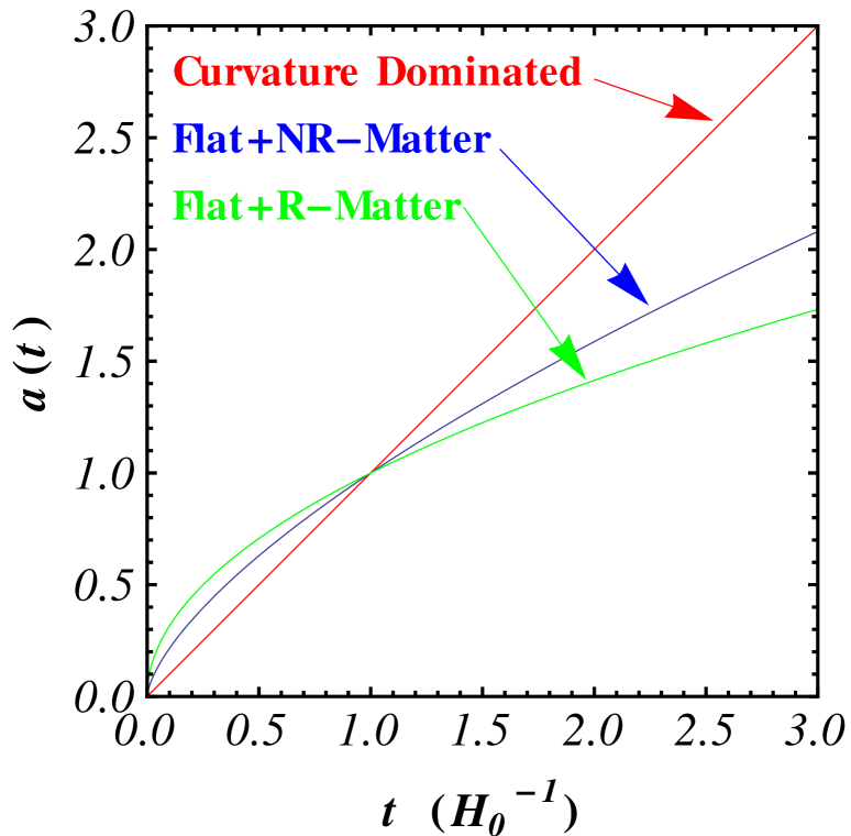
Figure 5: This figure shows the evolution of scale factor $a(t)$ as a function of cosmic time (in units of Hubble time) of single component Universes. The red line is for the Universe that is only curvature dominated (remember that according to Friedmann’s equation, a Universe with curvature only should be open, so $k=-1$) and scale factor behaves like $a(t)\propto t$. The scale factor as a function of time for the non-relativistic (NR) matter dominated Universe is shown as the blue curve. Mathematically $a(t)\propto t^{2/3}$. The relativistic (R) matter dominated Universe will expand as $a(t)\propto t^{1/2}$ and is shown as the green curve. All three Universes expand forever with no finite maximum value of scale factor.

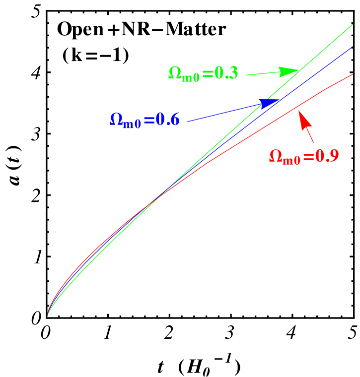
Figure 6: This figure shows the evolution of scale factor $a(t)$ as a function of cosmic time (in units of Hubble time) of open, non-relativistic (NR) matter dominated Universes, for three different values of $\Omega_{m0}$. It is clear from the plot that a larger value of $\Omega_{m0}$ decreases the rate of expansion of the Universe, but if $\Omega_{m0}<1$ the Universes is not only open, but will expand forever. All three Universes in this case will expand forever with no finite maximum values of scale factor. $\Omega_{m0}=0.3$ is the most realistic model of our Universe among the three models presented in this figure.

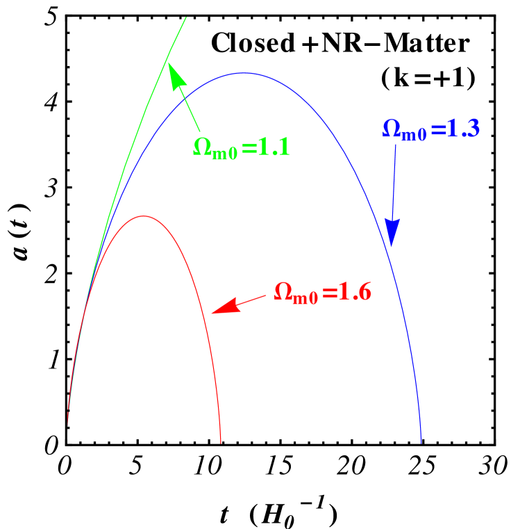
Figure 7: This figure shows the evolution of scale factor $a(t)$ as a function of cosmic time (in units of Hubble time) of closed, non-relativistic (NR) matter dominated Universes, for three different values of $\Omega_{m0}$. It is clear from the plots that a larger value of $\Omega_{m0}$ decreases the rate of expansion of the Universe. These Universes reach to a maximum scale factor of $a=a_{\mathrm{max}}=\frac{\Omega_{m0}}{2\left(\Omega_{m0}-1\right)}$ and then collapse to a big crunch. The larger the matter density, the faster the Universe will collapse (no surprise since collapse is due to the gravitational attraction between the matter in the Universe). All three Universes will eventually recollapse. The green curve that corresponds to the Universe having $\Omega_{m0}=1.1$, appears to indicate that it will continue expanding forever but if we increase the $t$ range of the plot, it too will come back to a big crunch, like the red and blue curves, but after a longer time.

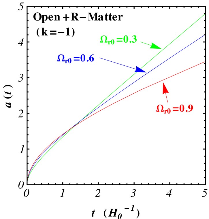
Figure 8: This figure shows the evolution of scale factor $a(t)$ as a function of cosmic time (in units of Hubble time) of open, relativistic (R) matter dominated Universes, for three different values of $\Omega_{r0}$. It is clear that a larger value of $\Omega_{r0}$ decreases the rate of expansion of the Universe, more than for the non-relativistic matter dominated case [see Fig. (6)], but if $\Omega_{r0}<1$ the Universe is not only open, but will expand forever. All three Universe in this case will expand forever with no finite value of scale factor.

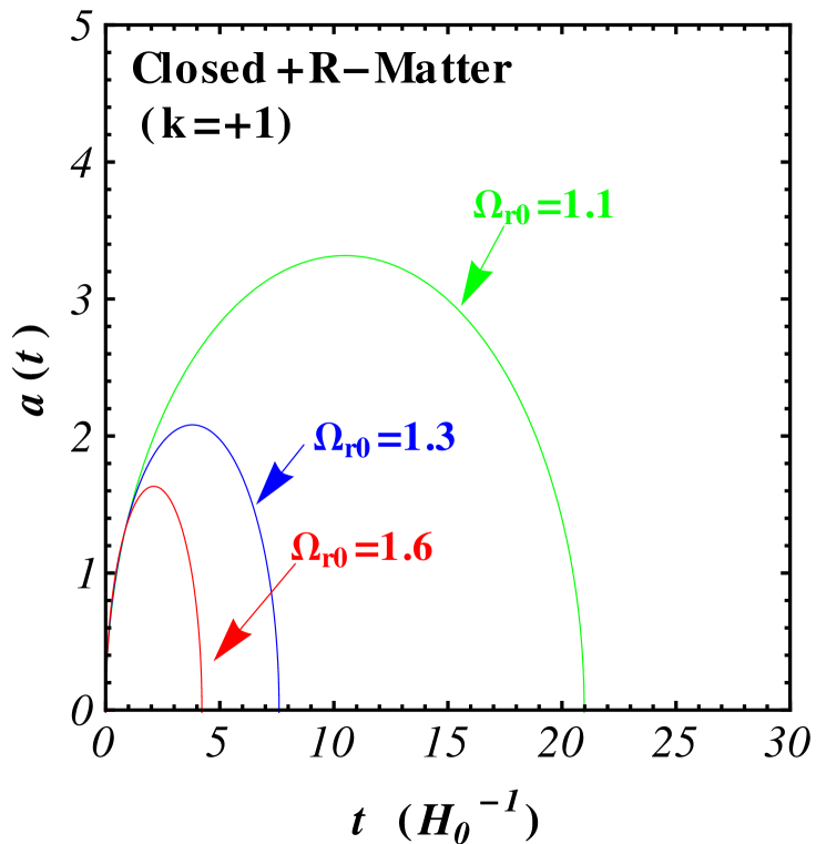
Figure 9: This figure shows the evolution of scale factor $a(t)$ as a function of cosmic time (in units of Hubble time) of closed, relativistic (R) matter dominated Universes, for three different values of $\Omega_{r0}$. It is clear that a larger value of $\Omega_{r0}$ decreases the rate of expansion of the Universe. These Universes reach maximum scale factor of $a=a_{\mathrm{max}}=\sqrt{\frac{\Omega_{r0}}{\Omega_{r0}-1}}$ and then collapse to a big crunch. The larger the radiation density faster the Universe will collapse. All three Universes will eventually recollapse.

Chapter 1 Distance Measures in Cosmology

In order to discuss and derive observational constraints on dark energy, it is important to introduce distance measures that are directly related to observations in the FLRW spacetime of Eq. (31).

In cosmology there are different ways to specify the distances between two points in space, is because different techniques can be used to define and measure the distance between two points! In addition in the expanding Universe the physical distance between co-moving objects changes and Earth-based observers look back in time as they look deep into space. We will define several different kinds of distances here. The commonality between all these different distances is that they are the measure of the separation between events on the radial null trajectories i.e., the trajectories of photons which terminate at the observer. In fact, a large part of the evidence for the existence of dark energy comes from the measurements of cosmological distances. Let’s start with the 4-dimensional

$$ds^{2} = g_{\mu\nu}dx^{\mu}dx^{\nu},$$ (1)

$$= -\mathrm{d}t^{2}+a^{2}(t)\mathrm{d}\sigma^{2},$$

$$= -\mathrm{d}t^{2}+a^{2}(t)\left[\mathrm{d}r^{2}+r^{2}\mathrm{d}\Omega^{2}\right],$$

$$= -\mathrm{d}t^{2}+a^{2}(t)\left[\mathrm{d}r^{2}+r^{2}\mathrm{d}\theta^{2}+r^{2}\mathrm{sin^{2}}\theta\mathrm{d}\phi^{2}\right],$$

where d$\sigma$ is the comoving spatial line element.

1 Comoving or Coordinate Distance

Let’s first discuss the comoving or coordinate distance which we denote by d_co. The co-moving distance d_co between two neighboring objects in the cosmos is the distance between them that remain constant with epoch if the two objects are moving only with the Hubble flow. This is the intuitive way of defining distance, but it is not directly measurable. In simple language, it is the distance between the two objects measured by a ruler at the time they were simultaneously observed (called proper or physical distance), divided by the ratio of the scale factor of the Universe then to now. So it is proper distance multiplied by $a_{0}/a=(1+z)$. The total line-of-sight comoving distance along a null geodesic can be found by setting $\mathrm{d}\Omega=0$, and $\mathrm{d}s=0$ in Eq. (1), then

$$\mathrm{d}_{co}(z)=R\ \chi=\int\limits^{t_{0}}_{t_{e}}\frac{\mathrm{d}t^{\prime}}{a(t^{\prime})}=\int\limits^{a_{0}}_{a_{e}}\frac{\mathrm{d}a}{a\dot{a}}=\frac{1}{a_{0}H_{0}}\int\limits^{z}_{0}\frac{\mathrm{d}z^{\prime}}{E(z^{\prime})},$$ (2)

where $t_{e}$ and $a_{e}$ is the cosmological time and scale factor at the time of emission of the photon from the source, similarly $t_{0}$ and $a_{0}$ are the values of cosmological time and scale factor at the time of observation and $z_{e}$ is the redshift of the source at the time of emission of the photon. According to convention $a_{0}=1$. $E(z)\equiv H(z)/H_{0}$ is the dimensionless Hubble parameter and $R\chi$, shown in the Fig. (1), is a comoving distance. $dt^{\prime}$ is the physical distance (remember $c$=1) traveled by photon in time $dt^{\prime}$, but dividing the physical distance by the scale factor $a(t^{\prime})$ we get the comoving distance, therefore $R\chi$ can be interpreted as the total, integrated comoving distance between the emitter and the observer. If the space is flat, this comoving distance is just the difference in the radial coordinates.

Figure 1: Two-dimensional FLRW geometry. This figure is taken from the Master’s thesis of Data Mania.¹⁰⁸

Although it is integrated over time for any two distinct galaxies moving with the Hubble flow, its value remains constant with time. It is just like the labels on a stretchable ruler: while the distance between two marks increases when the ruler is stretched,the labels remain the same.

The function $\int\limits^{z_{e}}_{0}\frac{\mathrm{d}z}{E(z)}$, can be expanded around $z_{e}=0$,

$$\int\limits^{z_{e}}_{0}\frac{\mathrm{d}z}{E(z)}\ \approx\ z_{e}-\frac{E^{\prime}(0)}{2}z_{e}^{2}+\frac{1}{6}\left[2E^{\prime 2}(0)+E^{\prime\prime}(0)\right]z_{e}^{3}+O(z_{e}^{4})+\cdots,$$ (4)

where a prime represents a derivative with respect to $z$.

For redshift $z$ much smaller than unity the comoving distance is approximately given from Eq. (2),

$$\mathrm{d}_{co}(z_{e})\approx\frac{1}{a_{0}H_{0}}z_{e},\hskip 56.9055pt(\mathrm{for}\ z_{e}\ll 1)$$ (5)

Since $z\approx v$, for a very small $z$, where $v$ is the speed of the source, we find

$$\mathrm{d}_{co}\approx\frac{1}{a_{0}H_{0}}v,$$ (6)

which is the Hubble law.

1 Some Insight: Start with 2-Dimensional Expansion

Let’s think about the homogeneous, isotropic expansion of a Universe with two spatial dimension (e.g., a 2-sphere embedded in three dimensional Euclidean space). We place dots (galaxies) on a balloon and allow it to expand see Fig. (2).

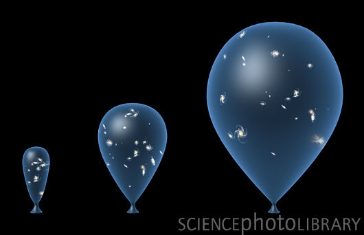
Figure 2: Hubble expansion in two spatial dimensions.

1. The spherical coordinates $(\theta,\phi)$ remain the same but the distance between points on the balloon changes in proportional to the scale factor $a(t)$. For concreteness think of the surface of earth, defined by latitudes and longitudes. Expand the size of globe (of course in imagination) by a factor of 2. The actual distance between two cities also increases by a factor of 2, but the $(\theta,\phi)$ coordinates of the two cities will remain unchanged.

2. An observer attached to a comoving coordinate (comoving or fundamental observer) sees all other points receding from him/her and sees a homogeneous, isotropic Universe.

3. An observer not comoving does not see an isotropic Universe.

4. The receding points maintain their comoving coordinates.

Some misconceptions

Although the balloon analogy is useful, one must guard against misconceptions that it can generate.

1. The surface that is expanding is two dimensional; the “center” of the balloon is in the third dimension and is not part of the surface, which has no center.

2. The balloon is expanded by the pressure difference between the inside and the outside, but the Universe is not being expanded by pressure.

3. Pressure couples to gravity in the Einstein equation, so the addition of (positive) pressure to the Universe would slow, not increase, the expansion rate see Eq. (235).

4. If the dots on the balloon represent galaxies, they too will expand. But real galaxies do not expand due to general Hubble expansion because they are gravitationally bound objects. We can make a better analogy by gluing solid objects (like 10 cent coins) to the surface of the balloon to represent galaxies, so that they do not expand when the balloon expands.

2 3-Dimensional Expansion

Now we can extend our understanding to 3-dimensional space expansion.

1. The coordinates $(r,\theta,\phi)$ of Friedmann-Lemaître-Robertson-Walker metric are comoving coordinates.

2. As the Universe expands (to the degree that peculiar motion relative to the Hubble flow can be ignored) comoving observer keeps the same coordinates $(r,\theta,\phi)$, and only the FLRW scale factor $a(t)$ changes with time.

3. Galaxies recede from us, but, if we are comoving observers, the receding galaxies maintain their comoving coordinates and the recession is described entirely by the time dependence of the scale factor $a(t)$.

4. Peculiar velocities will change the comoving coordinates, but these effects are small on large scales where the cosmological principle and therefore the FLRW metric is valid.

In some sense the comoving distance is the fundamental distance measure in cosmology, all others are expressed in terms of it.

2 Physical Distance

It is the actual proper distance, denoted by $r_{p}$, between the two objects in the cosmos that can be measured by a physical ruler. It is related to the co-moving distance d${}_{co}(z)$ through

$$r_{p}(z)=a(t)\mathrm{d}_{co}(z),$$ (7)

where $a(t)$ is the scale factor of the Universe. At the present epoch

$$r_{p}(z=0)=a(t_{0})\mathrm{d}_{co}(z).$$ (8)

Since $z\approx v$ for small values of $z$ and using Eq. (6), we have

$$r_{p}(z)\approx\frac{1}{H_{0}}v,\hskip 56.9055pt\mathrm{or}\ v\approx H_{0}r.$$ (9)

which means that Hubble’s law is satisfied. $v\propto z$ is only valid at small $z$. It is just a consequence of uniform expansion Hubble’s law that $v=H_{0}r$ is exactly always valid.

3 Transverse Comoving Distance

The comoving distance between two events at the same redshift or distance, but separated on the sky by some small angle $\phi$ is $r\phi$ where the transverse coordinate or comoving distance is denoted by $r$. In Fig. (1) it is $r=R\mathrm{sin}\chi$, so considering Eq. (2) we have

$$r(z)=\left\{\begin{array}[]{lc}\frac{1}{\sqrt{k}}\mathrm{sin}\left(\frac{\sqrt{k}}{a_{0}H_{0}}\int\limits^{z}_{0}\frac{dz^{\prime}}{E(z^{\prime})}\right)&\ \ \ \ \mathrm{for}\ k>0\\ \frac{1}{a_{0}H_{0}}\int\limits^{z}_{0}\frac{dz^{\prime}}{E(z^{\prime})}&\ \ \ \ \mathrm{for}\ k=0\\ \frac{1}{\sqrt{-k}}\mathrm{sinh}\left(\frac{\sqrt{-k}}{a_{0}H_{0}}\int\limits^{z}_{0}\frac{dz^{\prime}}{E(z^{\prime})}\right)&\ \ \ \ \mathrm{for}\ k<0\\ \end{array},\right.$$ (10)

where the trigonometric functions account for the curvature of space. Space curvature is not coordinate independent; a change of coordinates can make space flat. The only coordinate independent curvature is spacetime curvature, which is related to the local mass-energy density or really the stress-energy tensor.⁸¹ In terms of the curvature density parameter $\Omega_{k0}$, the coordinate distance can be written as

$$r(z)=\left\{\begin{array}[]{lc}\frac{1}{a_{0}H_{0}\sqrt{\Omega_{k0}}}\mathrm{sinh}\left(\sqrt{\Omega_{k0}}\int\limits^{z}_{0}\frac{dz^{\prime}}{E(z^{\prime})}\right)&\ \ \ \ \mathrm{for}\ \Omega_{k0}>0\\ \frac{1}{a_{0}H_{0}}\int\limits^{z}_{0}\frac{dz^{\prime}}{E(z^{\prime})}&\ \ \ \ \mathrm{for}\ \Omega_{k0}=0\\ \frac{1}{a_{0}H_{0}\sqrt{-\Omega_{k0}}}\mathrm{sin}\left(\sqrt{-\Omega_{k0}}\int\limits^{z}_{0}\frac{dz^{\prime}}{E(z^{\prime})}\right)&\ \ \ \ \mathrm{for}\ \Omega_{k0}<0\\ \end{array}.\right.$$ (11)

For $\Omega_{\Lambda}=0$, there is an analytical expression for the coordinate distance:^{120, 182}

$$r(z)=\frac{2\left[2-\Omega_{m0}(1-z)-(2-\Omega_{m0})\sqrt{1+\Omega_{m0}z}\ \right]}{a_{0}H_{0}\Omega^{2}_{m0}(1+z)}.$$ (12)

We stress here that coordinate distance $\boldsymbol{r}$ is not the proper distance — it is the proper distance divided by the ratio of the scale factor.

4 Dimensionless Coordinate Distance

It is useful to define the dimensionless coordinate distance denoted by $y(z)\equiv a_{0}H_{0}d_{m}(z)$,

$$y(z)=\left\{\begin{array}[]{lc}\frac{a_{0}H_{0}}{\sqrt{k}}\mathrm{sin}\left(\frac{\sqrt{k}}{a_{0}H_{0}}\int\limits^{z}_{0}\frac{dz^{\prime}}{E(z^{\prime})}\right)&\ \ \ \ \mathrm{for}\ k>0\\ \int\limits^{z}_{0}\frac{dz^{\prime}}{E(z^{\prime})}&\ \ \ \ \mathrm{for}\ k=0\\ \frac{a_{0}H_{0}}{\sqrt{-k}}\mathrm{sinh}\left(\frac{\sqrt{-k}}{a_{0}H_{0}}\int\limits^{z}_{0}\frac{dz^{\prime}}{E(z^{\prime})}\right)&\ \ \ \ \mathrm{for}\ k<0\\ \end{array}.\right.$$ (13)

In terms of the curvature density parameter $\Omega_{k0}$, it is given by

$$y(z)=\left\{\begin{array}[]{lc}\frac{1}{\sqrt{\Omega_{k0}}}\mathrm{sinh}\left(\sqrt{\Omega_{k0}}\int\limits^{z}_{0}\frac{dz^{\prime}}{E(z^{\prime})}\right)&\ \ \ \ \mathrm{for}\ \Omega_{k0}>0\\ \int\limits^{z}_{0}\frac{dz^{\prime}}{E(z^{\prime})}&\ \ \ \ \mathrm{for}\ \Omega_{k0}=0\\ \frac{1}{\sqrt{-\Omega_{k0}}}\mathrm{sin}\left(\sqrt{-\Omega_{k0}}\int\limits^{z}_{0}\frac{dz^{\prime}}{E(z^{\prime})}\right)&\ \ \ \ \mathrm{for}\ \Omega_{k0}<0\\ \end{array}.\right.$$ (14)

5 Angular Diameter Distance

The angular diameter distance, $d_{A}$, is the ratio of an object’s physical transverse size, denoted by $l_{\perp}$, to its angular size (in radians). See Fig. (1). Mathematically,

$$d_{A}(z)=\frac{l_{\perp}}{\phi}=\frac{ar(z)\phi}{\phi}=ar(z)=\frac{a_{0}r(z)}{1+z}.$$ (15)

In terms of dimensionless coordinate distance it is given as,

$$d_{A}(z)=\frac{y(z)}{H_{0}(1+z)}.$$ (16)

This distance is often used when discussing CMB anisotropies observations.

6 Luminosity Distance

The luminosity distance denoted by $d_{L}$ is defined by the relations between the bolometric (i.e. integrated over all frequencies) flux $\mathcal{F}$ and the bolometric absolute luminosity $L$ (defined as the total power radiated in watts). It is a measure of how far an object of known luminosity $L$ is that produces the luminosity flux of $\mathcal{F}$, assuming the inverse-square law,

$$\mathcal{F} = \frac{L}{4\pi d^{2}_{L}}\ ,$$ (17)

$$\Rightarrow\hskip 14.22636ptd_{L} = \sqrt{\frac{L}{4\pi\mathcal{F}}}\ .$$ (18)

Note that the observed luminosity (that we will denote as $L_{0}$), which is luminosity detected at d${}_{co}=0$ ($z=0$), is different from the absolute luminosity $L$ of the source (emitted at a comoving distance d_co with redshift $z$). Thus $d_{L}$ can be found from measurements of $\mathcal{F}$, provided $L$ is known; the trouble is that generally, it is not. However, there are certain classes of objects for which we do know $L$, to some accuracy, and all higher levels of the cosmic distance ladder are based on these “standard candles”.

The flux $\mathcal{F}$ is defined by $\mathcal{F}=L_{0}/S$, where $S$ is the surface area over which that flux is spread and it is equal to $S=4\pi(a_{0}r)^{2}$ (area of the sphere at $z=0$). Then from Eq. (18):

$$\mathcal{F}=\frac{L}{4\pi d^{2}_{L}}=\frac{L_{0}}{4\pi(a_{0}r)^{2}},$$ (19)

$$\Rightarrow\hskip 14.22636ptd^{2}_{L}=(a_{0}r)^{2}\frac{L}{L_{0}}.$$ (20)

Now, we need to find the ratio $\frac{L}{L_{0}}$ in terms of known quantities.

If energy $\Delta E_{e}$ is emitted in time interval $\Delta t_{e}$ from a distinct object (with redshift $z$), then the absolute luminosity is

$$L=\frac{\Delta E_{e}}{\Delta t_{e}}.$$ (21)

The flux of this energy observed at $z=0$, denoted by $L_{0}$, is

$$L_{0}=\frac{\Delta E_{0}}{\Delta t_{0}},$$ (22)

where $\Delta E_{0}$ is the energy of light detected during time interval $\Delta t_{0}$. From Planck’s theory, the energy of the photon is inversely proportional to it’s wavelength $\lambda$ $\left(E={hc}/{\lambda}\right)$, hence,

$$\frac{\Delta E_{e}}{\Delta E_{0}}=\frac{\lambda_{0}}{\lambda_{e}}=1+z,$$ (23)

where $\lambda_{e}$ and $\lambda_{0}$ are the wavelengths of the light at the point of emission (at redshift $z$) and detection (at $z=0$) respectively, and we have used Eq. (159) in the second step, Also, since $c=\frac{\lambda}{\Delta t}$,

$$\frac{\lambda_{e}}{\Delta t_{e}}=\frac{\lambda_{0}}{\Delta t_{0}},$$ (24)

$$\Rightarrow\hskip 14.22636pt\frac{\lambda_{0}}{\lambda_{e}}=\frac{\Delta t_{0}}{\Delta t_{e}}=1+z,$$ (25)

and so,

$$\frac{L_{e}}{L_{0}} = \frac{\Delta E_{e}}{\Delta t_{e}}\cdot\frac{\Delta t_{0}}{\Delta E_{0}}=\frac{\Delta E_{e}}{\Delta E_{0}}\cdot\frac{\Delta t_{0}}{\Delta t_{e}},$$ (26)

$$= (1+z)\cdot(1+z).\hskip 56.9055pt(\mathrm{using}\ \mathrm{Eq.}\ (\ref{eq:ldq7})-(\ref{eq:ldq8}))$$

Hence, from Eq. (20),

$$d^{2}_{L} = (a_{0}r)^{2}(1+z)^{2}.$$ (27)

Taking the square root on both sides we will get:

$$d_{L} = (a_{0}r)(1+z).$$ (28)

In terms of the dimensionless coordinate distance, the luminosity distance is,

$$d_{L} = \frac{1}{H_{0}}y(z)(1+z),$$ (29)

so the luminosity distance can be expressed using Eq. (14) in terms of curvature density parameter as

$$d_{L}(z)=\left\{\begin{array}[]{lc}\frac{(1+z)}{H_{0}\sqrt{\Omega_{k0}}}\mathrm{sinh}\left(\sqrt{\Omega_{k0}}\int\limits^{z}_{0}\frac{dz^{\prime}}{E(z^{\prime})}\right)&\ \ \ \ \mathrm{for}\ \Omega_{k0}>0\\ \frac{1+z}{H_{0}}\int\limits^{z}_{0}\frac{dz^{\prime}}{E(z^{\prime})}&\ \ \ \ \mathrm{for}\ \Omega_{k0}=0\\ \frac{(1+z)}{H_{0}\sqrt{-\Omega_{k0}}}\mathrm{sin}\left(\sqrt{-\Omega_{k0}}\int\limits^{z}_{0}\frac{dz^{\prime}}{E(z^{\prime})}\right)&\ \ \ \ \mathrm{for}\ \Omega_{k0}<0\\ \end{array}\right.$$ (30)

and using Eq. (13)in terms of curvature parameter as,

$$d_{L}(z)=\left\{\begin{array}[]{lc}\frac{a_{0}(1+z)}{\sqrt{k}}\mathrm{sin}\left(\frac{\sqrt{k}}{a_{0}H_{0}}\int\limits^{z}_{0}\frac{dz^{\prime}}{E(z^{\prime})}\right)&\ \ \ \ \mathrm{for}\ \ k>0\\ \frac{1+z}{H_{0}}\int\limits^{z}_{0}\frac{dz^{\prime}}{E(z^{\prime})}&\ \ \ \ \mathrm{for}\ \ k=0\\ \frac{a_{0}(1+z)}{\sqrt{-k}}\mathrm{sinh}\left(\frac{\sqrt{-k}}{a_{0}H_{0}}\int\limits^{z}_{0}\frac{dz^{\prime}}{E(z^{\prime})}\right)&\ \ \ \ \mathrm{for}\ \ k<0\\ \end{array}\right.$$ (31)

Now let’s compute the approximate expression for the luminosity distance when $z\ll 1$, that we will use in Chapter (2) where we will calculate the general expression of luminosity distance as a function of $z\ll 1$ in non-flat Universe having dark energy. In order to do this we read the Maclaurin series expansion of the integral $\int\limits^{z}_{0}\frac{dz^{\prime}}{E(z^{\prime})}$,

$$\int\limits^{z}_{0}\frac{dz^{\prime}}{E(z^{\prime})}\ \ =\ z-\frac{E^{\prime}(0)}{2}z^{2}+\frac{1}{6}\left[2E^{\prime}(0)^{2}-E^{\prime\prime}(0)\right]z^{3}+O(z^{4}).$$ (32)

Now using the expansion of sinh($x$)$=x+\frac{x^{3}}{6}+O(x^{5})$, we get from Eq. (30),

$$d_{L}(z)\ = \ \frac{(1+z)}{H_{0}\sqrt{\Omega_{k0}}}\ \mathrm{sinh}\left[\sqrt{\Omega_{k0}}\left(z-\frac{E^{\prime}(0)}{2}z^{2}+\frac{1}{6}\left[2E^{\prime}(0)^{2}-E^{\prime\prime}(0)\right]z^{3}+O(z^{4})\right)\right],$$ (33)

$$= \ \frac{(1+z)}{H_{0}\sqrt{\Omega_{k0}}}\ \left[\sqrt{\Omega_{k0}}\left(z-\frac{E^{\prime}(0)}{2}z^{2}+\frac{1}{6}\left[2E^{\prime}(0)^{2}-E^{\prime\prime}(0)\right]z^{3}\right)\vphantom{\frac{(\Omega_{k0})^{3/2}z^{3}}{6}}\right.$$

$$\hskip 62.59596pt+\ \left.\frac{(\Omega_{k0})^{3/2}z^{3}}{6}+\dots\right],$$

$$\approx \frac{(1+z)}{H_{0}\cancel{\sqrt{\Omega_{k0}}}}\ \ \cancel{\sqrt{\Omega_{k0}}}\left[z-\frac{E^{\prime}(0)}{2}z^{2}+\frac{1}{6}\left[2E^{\prime}(0)^{2}-E^{\prime\prime}(0)+\Omega_{k0}\right]z^{3}\right],$$

$$\approx \frac{1}{H_{0}}\left[z+z^{2}-\frac{E^{\prime}(0)}{2}z^{2}-\frac{E^{\prime}(0)}{2}z^{3}+\frac{1}{6}\left(2E^{\prime}(0)^{2}-E^{\prime\prime}(0)+\Omega_{k0}\right)z^{3}\right].$$

$$= \frac{1}{H_{0}}\left[z+\left(1-\frac{E^{\prime}(0)}{2}\right)z^{2}+\frac{1}{6}\left(2E^{\prime}(0)^{2}-3E^{\prime}(0)-E^{\prime\prime}(0)+\Omega_{k0}\right)z^{3}\right].$$

Reintroducing the speed of light is $c$, the approximate luminosity distance for $z\ll 1$ is,

$$d_{L}(z) \approx \frac{c}{H_{0}}\left[z+\left(1-\frac{E^{\prime}(0)}{2}\right)z^{2}+\frac{1}{6}\left(2E^{\prime}(0)^{2}-3E^{\prime}(0)-E^{\prime\prime}(0)+\Omega_{k0}\right)z^{3}\right].$$ (34)

We can relate the angular diameter distance $d_{A}$ and the luminosity distance using Eq. (16), and (29),

$$d_{A}(z) = \frac{y(z)}{H_{0}(1+z)}=\frac{d_{L}(z)}{(1+z)^{2}}.$$ (35)

7 Distance Modulus

The apparent magnitude, $m$, of an astronomical object is defined by the ratio of the apparent flux of the object to some reference flux,

$$m=-2.5\ \mathrm{log_{10}}\left(\frac{\mathcal{F}}{\mathcal{F}_{\mathrm{ref}}}\right).$$ (36)

The absolute magnitude, $M$, is defined as the apparent magnitude the object would have if it were 10 pc away. The difference between them is known as distance modulus and can be expressed as:

$$\mu\equiv m-M = -2.5\ \mathrm{log_{10}}\left(\frac{\mathcal{F}}{\mathcal{F}_{\mathrm{ref}}}\right)-(-2.5)\ \mathrm{log_{10}}\left(\frac{\mathcal{F}_{\mathrm{10\ pc}}}{\mathcal{F}_{\mathrm{ref}}}\right),$$ (37)

$$= -2.5\ \mathrm{log_{10}}\left(\frac{\mathcal{F}}{\mathcal{F}_{\mathrm{10\ pc}}}\right),$$

$$= -2.5\ \mathrm{log_{10}}\left(\frac{L}{4\pi d_{L}^{2}}\cdot\frac{4\pi(10\ \mathrm{pc})^{2}}{L}\right),$$

$$= -2.5\ \mathrm{log_{10}}\left(\frac{10\ \mathrm{pc}}{d_{L}}\right)^{2},$$

$$= 5\ \mathrm{log_{10}}\left(\frac{d_{L}}{\mathrm{10\ pc}}\right).$$

Let’s write this distance modulus in terms of dimensionless coordinate distance $y(z)$, as a function of the dimensionless Hubble parameter, using Eq. (29),

$$\mu=5\ \mathrm{log_{10}}\left(\frac{d_{L}}{\mathrm{10\ pc}}\right)=5\ \mathrm{log_{10}}\left[\frac{c}{H_{0}}y(z)(1+z)\frac{1}{\mathrm{10\ pc}}\right].$$ (39)

Now, with the value of $c=3\times 10^{5}$ km s^-1, and $H_{0}=h$($100$ km s^-1 Mpc^-1), we get

$$\mu(z,h) = 5\ \mathrm{log_{10}}\left[\frac{3\times 10^{5}\ \mathrm{km\ s^{-1}}}{\frac{100h\ \mathrm{km\ s^{-1}}}{10^{6}\ \mathrm{pc}}}y(z)(1+z)\frac{1}{10\ \mathrm{pc}}\right],$$ (40)

$$= 5\ \mathrm{log_{10}}\left[\frac{3\times 10^{8}}{h}y(z)(1+z)\right],$$

$$= 5\ \mathrm{log_{10}}\Big{[}3000y(z)(1+z)\Big{]}+25-5\ \mathrm{log_{10}}(h).$$

This is the equation we will use in the supernova (SN) analyses in Chapter (4).

Chapter 2 Dark Energy and Dark Energy Models

In this chapter we will discuss two commonly used dark energy models, and one dark energy parametrization, but prior to that we discuss the observational evidence for most mysterious type od substance i.e., dark energy.

1 Observational Evidence for Dark Energy

From the last two decades, evidence for the most striking results in modern cosmology has been steadily growing, namely the existence of a cosmological constant or dark energy, which is believed to be the cause of the current accelerated expansion of the Universe as first observed by Perlmutter et al.,¹²⁷ and Riess et al.¹⁴⁴ Although it may not have come as such a surprise to a few theorists, who were at that time considering the interplay between a number of different types of observations,^{91, 121, 119, 139} for the majority it came as something of a bombshell. The Universe is not only expanding, it is expanding with acceleration. The results first published by Perlmutter et al.,¹²⁷ and Riess et al.¹⁴⁴ where the one that caused a major change in the way we have started thinking about the universe.

There is a key problem that we have to explain, and it is fair to say it has yet to be understood. The value of the energy density stored in the cosmological constant or dark energy today (the assumed cause of accelerated expansion), has to be of order of the critical density, namely $\rho_{\Lambda}\sim 10^{-3}\,{\rm eV}^{4}$. It is unfortunate that no reasonable explanation exists as to why a true cosmological constant should be at this scale. There are reasons to think it should naturally be much larger. Typically, since it is conventionally associated with the energy of the vacuum in quantum field theory, we expect it to have a magnitude of order the typical energy scale of early Universe phase transitions. Even the QCD scale, it would imply a much larger value, $\rho_{\Lambda}\sim 10^{-3}\,{\rm GeV}^{4}$. The question then remains, why does $\Lambda$ have the value that it has today?

In order to explain the current accelerated expansion of the universe, we require an exotic substance dubbed “dark energy” with an equation-of-state parameter satisfying $\omega<-1/3$, as mentioned in Eq. (251). Newtonian gravity cannot account for the accelerated expansion, it allows only decelerated cosmological expansion. Let’s consider a homogeneous sphere with radius $a$ and energy density $\rho$. The Newton’s equation of motion for a point particle with mass $m$ on this sphere is

$$F = -\frac{GMm}{a^{2}},$$

$$m\ddot{a} = -\frac{Gm}{a^{2}}\left(\frac{4\pi a^{3}\rho}{3}\right)\ ,\hskip 28.45274pt\left(\mathrm{Here},\ M=\rho V=\frac{4\pi a^{3}\rho}{3}\right)$$

$$\Rightarrow\ \ \ \frac{\ddot{a}}{a} = -\frac{4\pi G}{3}\rho\,.$$ (1)

The difference compared to the Einstein’s equation (236) is the absence of the pressure term, $P$. This appears in Einstein’s equation because of relativistic effects. The condition $\omega<-1/3$ means that we essentially require a large negative pressure in order to give rise to an accelerated expansion.

Now let’s consider mathematically how to accommodate energy with $\omega<-1/3$ in Friedmann’s equations. From Eq. (139), the energy density $\rho$ is constant with respect to cosmological time $t$ for a fluid which has $\omega=-1$. In this case, in a spatially-flat model, the Hubble rate, $\dot{a}/a$ in Eq. (236) also is constant. This leads to the exponential evolution of the scale factor with respect to time,

$$a(t)\propto e^{Ht}.$$ (2)

This is the de Sitter spacetime or Universe. As we will see in a later section, this exponential expansion also arises in the Einstein equations in the case of the cosmological constant $\Lambda$ dominant Universe.

We now discuss some of the observational facts in the support of the existence of dark energy. These include:

• The age of the Universe compared to that of the oldest star in combination with estimate of $H_{0}$.

• Supernovae apparent magnitude observations (SNeIa).

• Cosmic microwave background (CMB) anisotropy observations in combination with the estimation of $\Omega_{m0}$, the non relativistic matter density parameter.

• Baryonic acoustic oscillation (BAO) peak length scale measurements.

• Hubble parameter measurements.

• Large-scale-structure (LSS) observations.

Even in the last two decades of the $20^{th}$ century, there were some observations that the age of a cold dark matter (CDM) dominated Universe with $\Omega_{m0}=1$ was smaller than the age of the oldest stars in globular clusters in our Milky Way galaxy. Adding dark energy and so reducing the amount of CDM, can address this apparent inconsistency by increasing the age of the Universe. The stronger evidence supporting accelerated cosmological expansion (and consequently the presence of dark energy along with that of CDM) came from measurements of the luminosity distance of type Ia Supernovae (SNeIa). CMB observations also favor the presence of the dark energy, yet the constraints obtained from CMB alone on dark energy are very weak. The BAO measurements are another independent source of support for the idea of the dark energy, as are $H(z)$ measurements. The last idea that we will discuss is that that power spectrum density irregularities is also consistent with the existence of dark energy. We now discuss some of these observations in a little more detail.

1 Age of the Universe

By looking at Table. (4) in which the age of the Universe $t_{0}$ is given in terms of the inverse of the Hubble constant $H^{-1}_{0}$ for single-component Universes, it is easy to see that dimensionally $H_{0}^{-1}$ sets the scale for $t_{0}$ and we expect this to be the case in multiple components Universes, like ours, also. In this Section we try to make a more precise guess (estimate of $H_{0}$ by incorporating factors that we have previously ignored) and then will compare this to $t_{0}$ the age of the oldest known stars. We now consider dark energy, thus with the time dependent dark energy density $\rho_{DE}(t)$ and using Eq. (141) write

$$\dot{\rho}_{DE}(t)=3\left(\frac{\dot{a}}{a}\right)\Big{(}\rho_{DE}(t)+P_{DE}(t)\Big{)}.$$ (3)

We assume a dark energy equation-of-state-parameter $\omega_{DE}$ which is time dependent so,

$$P_{DE}(t)=\omega_{DE}(t)\ \rho_{DE}(t).$$ (4)

Equation (3) then takes the form

$$\frac{\dot{\rho}_{DE}(t)}{\rho_{DE}(t)}=3\left(\frac{\dot{a}}{a}\right)\Big{(}1+\omega_{DE}(t)\Big{)}.$$ (5)

or,

$$\frac{d\rho_{DE}}{\rho_{DE}}=3\left(1+\omega_{DE}\right)\frac{da}{a}.$$ (6)

Integrating from some time in the past to the present when $a_{0}=1$,

$${\int}\frac{d\rho_{DE}}{\rho_{DE}}=\int\limits^{1}_{a}3\left(1+\omega_{DE}\right)\frac{da^{\prime}}{a^{\prime}}+\mathrm{ln}\rho_{DE,0}\ ,$$ (7)

where ln$\rho_{DE,0}$ is the constant of integration. Substituting:

$$a^{\prime}=\frac{1}{1+z},\hskip 28.45274pt\ \ \ \ \ \hskip 28.45274ptda^{\prime}=-\frac{1}{(1+z)^{2}}dz,$$ (8)

$$\Rightarrow\ \ \ {\int}\frac{d\rho_{DE}}{\rho_{DE}} = \int\limits^{0}_{z}-3\frac{\left(1+\omega_{DE}(z^{\prime})\right)}{1+z^{\prime}}dz^{\prime}+\mathrm{ln}\rho_{DE,0}\ ,$$ (9)

$$\Rightarrow\ \ \ \mathrm{ln}\rho_{DE} = \int\limits^{z}_{0}\frac{3\left(1+\omega_{DE}(z^{\prime})\right)}{1+z^{\prime}}dz^{\prime}+\mathrm{ln}\rho_{DE,0},$$ (10)

Thus we will get redshift $z$ dependent dark energy density

$$\rho_{DE}(z)=\rho_{DE,0}\ \mathrm{exp}\left[\int\limits^{z}_{0}\frac{3\left(1+\omega_{DE}(z^{\prime})\right)}{1+z^{\prime}}dz^{\prime}\right].$$ (11)

Which can also be written by introducing a average $\langle\omega_{DE}\rangle$ as:

$$\rho_{DE}(z)=\rho_{DE,0}(1+z)^{3(1+\langle\omega_{DE}\rangle)}.$$ (12)

Where $\langle\omega_{DE}\rangle$ is defined as:

$$\langle\omega_{DE}\rangle=\frac{1}{\mathrm{ln}(1+z)}\int\limits^{z}_{0}\frac{\omega_{DE}(z^{\prime})}{1+z^{\prime}}dz^{\prime}.$$ (13)

If we will take into account other components like radiation, non-relativistic matter, and space curvature, then Eq. (271) is of the from:

$$H^{2}=\frac{8\pi G}{3}\left(\rho_{r}+\rho_{m}+\rho_{DE}\right)-\frac{k}{a^{2}}.$$ (14)

Present epoch density parameters, defined in Eq. (277), obey

$$\Omega_{m0}+\Omega_{r0}+\Omega_{k0}+\Omega_{DE,0}=1,$$ (15)

so we can rewrite Eq. (14) in the form, $H^{2}(z)=H_{0}^{2}E^{2}(z)$, Where $E(z)\equiv H(z)/H_{0}$ is

$$E^{2}(z) = \left[\Omega_{r0}(1+z)^{4}+\Omega_{m0}(1+z)^{3}\hskip 85.35826pt\vphantom{\left\{\int\limits^{z}_{0}\frac{3(1+\omega_{DE})}{1+z^{\prime}}\mathrm{d}z^{\prime}\right\}}\right.$$ (16)

$$\left.+\ \Omega_{DE,0}\ \mathrm{exp}\left\{3\int\limits^{z}_{0}\frac{(1+\omega_{DE}(z^{\prime}))}{1+z^{\prime}}\mathrm{d}z^{\prime}\right\}+\Omega_{k0}(1+z)^{2}\right].$$

Since $H={\dot{a}}/{a}$, $a={1}/({1+z})$ $\Rightarrow$ $H=-\dot{z}/{(1+z)}$, the age of the Universe can be expressed as

$$t_{0}=\frac{1}{H_{0}}\int\limits^{\infty}_{0}\frac{dz}{E(z)(1+z)}.$$ (17)

This integral is dominated by the terms at low redshift. Since $\Omega_{r0}$ is of the order of $10^{-4}$, for detail see,^{147, 137, 98, 182, 89, 115} radiation will play an important role only at high redshifts $z\gtrsim 1000$. Hence for the sake of simplicity we ignore radiation when evaluating Eq. (17) then Eq. (15) reduced to $\Omega_{m0}+\Omega_{DE,0}+\Omega_{K0}=1$.

Let’s consider the special case of time independent $\omega_{DE}=-1$ (Einstein’s cosmological constant). Then the age of the Universe is

$$t_{0}=\frac{1}{H_{0}}{{\int}}\limits_{0}^{\infty}\frac{dz}{(1+z)\Big{[}\Omega_{m0}(1+z)^{3}+\Omega_{DE,0}+\Omega_{K0}(1+z)^{2}\Big{]}^{1/2}}.$$ (18)

Further simplifying $t_{0}$ the flat case (with $\Omega_{K0}=0$, and so $\Omega_{DE,0}=1-\Omega_{m0}$), and substituting

$$(1+z)^{3}=\frac{1-\Omega_{m0}}{\Omega_{m0}}\ \mathrm{sinh^{2}}\beta,\hskip 28.45274pt\mathrm{d}z=\frac{2}{3}\left(\frac{1-\Omega_{m0}}{\Omega_{m0}}\right)^{1/3}\mathrm{sinh^{-1/3}}\beta\ \mathrm{cosh}\beta\ \mathrm{d}\beta,$$ (19)

Then the integral Eq. (18) becomes,

$$t_{0}=\frac{2}{3H_{0}\sqrt{1-\Omega_{m0}}}\int\limits_{\mathrm{sinh^{-1}}\left[\sqrt{\frac{\Omega_{m0}}{1-\Omega_{m0}}}\ \right]}^{\infty}\mathrm{cosech}\beta\ \mathrm{d}\beta,$$ (20)

which can be easily integrated, and in terms of $\Omega_{m0}$ gives,

$$t_{0}=\frac{1}{3H_{0}\sqrt{1-\Omega_{m0}}}\mathrm{ln}\Bigg{(}\frac{1+\sqrt{1-\Omega_{m0}}}{1-\sqrt{1-\Omega_{m0}}}\Bigg{)}.$$ (21)

In the limit $\Omega_{DE,0}\rightarrow 0$, we have our old result for Einstein-de Sitter model derived in Eq. (264):

$$t_{0}=\frac{2}{3H_{0}}.$$ (22)

Using the then-favored dimensionless Hubble parameter value $h=0.72\pm 0.08$ (today $h=0.68\pm 0.028$ is probably a batter estimate see ^{83, 41}) the age of the Universe in the absence of the cosmological constant is in the range $8.2\ \mathrm{Gyr}\ \leqslant t_{0}\leqslant 10.2\ \mathrm{Gyr}$ ($9.2\ \mathrm{Gyr}\leqslant t_{0}\leqslant 10.2\ \mathrm{Gyr}$). So this is the theoretical value we have. On the other hand, Carretta et al. ³⁵ estimated the age of a globular cluster in the Milky Way galaxy to be $12.9\pm 2.9$ Gyr. Jimenez et al. ⁸⁷ calculated the value of $13.5\pm 2$ Gyr, whereas Hansen et al.⁷⁹ constrained the age of the globular cluster Messier 4 (M$4$) to be $12.7\pm 0.7$ Gyr by using the method of the white dwarf cooling sequence. Overall, observations of the ages of the globular clusters are larger than about 11 Gyr. Consequently, this leads to some doubt about the numerical age of the Universe results obtained in the Einstein-de Sitter model from Eq. (22).

One of the ways to address this problem is to take a cosmological constant (or dark energy with an equation-of-state-parameter $\omega_{DE}\approx-1$) into account. From Eq. (21) it is clear that $t_{0}$ increases with the decrease of $\Omega_{m0}$. The limit $\Omega_{m0}\rightarrow 0$ results in $t_{0}\rightarrow\infty$.

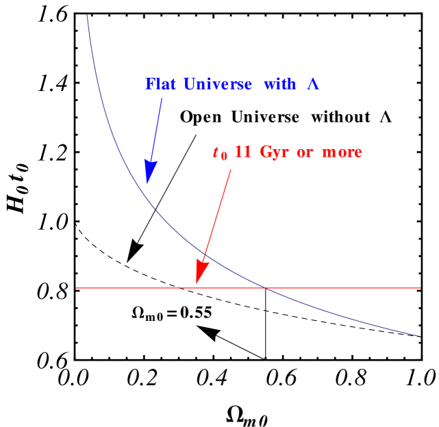
Figure 1: The cosmic age $t_{0}$ in terms of $H^{-1}_{0}$ verses $\Omega_{m0}$. The thin-solid blue curve describes a flat Universe in the presence of the cosmological constant $\Lambda$ with the constraints $\Omega_{m0}+\Omega_{DE,0}=1$. The dashed black curve corresponds to an open Universe without the cosmological constant $\Lambda$. The red horizontal line is a minimum age of the Universe allowed to form the oldest globular cluster ($>$11 Gyr), here we suppose $H_{0}=72\pm 8$ km s^-1 Mpc^-1. Here the intersection of the blue line and red line is at $\Omega_{m0}=0.55$, which gives the constraint that $\Omega_{m0}<0.55$ if the age of the spatially-flat with dark energy Universe has to be more than the age of the oldest globular clusters.

Figure (1) shows the cosmic age predicted by Eq. (21) as a function of $\Omega_{m0}$. It shows that if the $t_{0}$ must be greter than 11 Gyr then $\Omega_{m0}<0.55$. The WMAP 5-year estimates on the cosmic age (assuming the $\Lambda$CDM model) is $t_{0}=13.73\pm 0.12$ Gyr.⁹⁰ Under this bound we find that the density parameter of non-relativistic matter is constrained to be $0.245<\Omega_{m0}<0.261$ for $h=0.72$. When $h=0.68$ then $0.27<\Omega_{m0}<0.29$.⁶¹

We only considered the flat case and we showed that the way to increase the cosmic age of Universe is by incorporating dark energy (the cosmological constant), but what if we will consider an open Universe, i.e. let $\Omega_{K0}>0$? To address this issue we have to integrate Eq. (18) without incorporating dark energy, with positive curvature density ($\Omega_{K0}>0$). Hence, $\Omega_{m0}+\Omega_{K0}=1$. substituting

$$1+z=\frac{1-\Omega_{m0}}{\Omega_{m0}}\ \mathrm{sinh^{2}}\beta,\hskip 28.45274pt\mathrm{d}z=2\left(\frac{1-\Omega_{m0}}{\Omega_{m0}}\right)\mathrm{sinh}\beta\ \mathrm{cosh}\beta\ \mathrm{d}\beta,$$ (23)

in Eq. (18)the equation becomes

$$t_{0}=\frac{2\ \Omega_{m0}}{H_{0}\left(1-\Omega_{m0}\right)^{3/2}}\int\limits_{\mathrm{sinh^{-1}}\left[\sqrt{\frac{\Omega_{m0}}{1-\Omega_{m0}}}\ \right]}^{\infty}\mathrm{cosech^{3}}\beta\ \mathrm{d}\beta,$$ (24)

which is easily integrated and in terms of $\Omega_{m0}$, we get

$$t_{0}=\frac{1}{H_{0}(1-\Omega_{m0})}\left[1+\frac{\Omega_{m0}}{2\sqrt{1-\Omega_{m0}}}\mathrm{ln}\Bigg{(}\frac{1-\sqrt{1-\Omega_{m0}}}{1-\sqrt{1+\Omega_{m0}}}\Bigg{)}\right].$$ (25)

The dashed black lines in Fig. (1) show the age of the open Universe without incorporating dark energy. In the limit $\Omega_{m0}\rightarrow 1$, we recover the value in Eq. (22) in the flat Universe. On the other hand, in the limit $\Omega_{m0}\rightarrow 0$, we have $t_{0}\rightarrow H_{0}^{-1}$. So we can conclude that the cosmic age of the open Universe does not become as large as in the case of flat Universe with dark energy (cosmological constant). Since the curvature $|\Omega_{K0}|$ has been constrained to be much smaller then unity from WMAP measurements,⁹⁰ it is almost impossible to satisfy the condition $t_{0}>11$ Gyr for $h=0.72\pm 0.08$ in the open Universe without dark energy.

The above discussion shows that the existence of dark energy can resolve the cosmic age problem.

2 Supernovae Apparent Magnitude Observations (SNeIa)

Persuasive evidence for the current cosmic acceleration, and hence for dark energy, came from observations of the distance modulus of distant supernova of type Ia (SNIa). Two independent groups working on observations of supernovae [Riess et al. named the High-Redshift Supernovae Search Team (HSST)¹⁴⁴ and Perlmutter et al. named the Supernovae Cosmology Project (SCP)¹²⁷] reported late time cosmic acceleration. By 1998 Riess et al. has studied 16 high-redshift SNIa along with the 34 nearby supernovae, while by 1999 the SCP group had studied 42 SNIa in the redshift range $0.18\leq z\leq 0.83$.

The supernova explosion, in which large amounts of energy are released as electromagnetic radiation to interstellar space, can be triggered in two ways. In both ways, it is gravity that gives a SN its energy.

1. By the abrupt reignition of nuclear fusion in a compact star. The compact star may accumulate sufficient material from it’s surroundings, either by a merger or through accretion, to raise its core temperature and ignite nuclear fusion, completely disrupting the star.

2. By the collapse of the core of the massive star. Mass flows into the core of the star by the continued formation of iron from nuclear fusion. Once the core has gained so much mass that it cannot withstand its own weight (gravity), the core implodes. This implosion can some time be halted by neutron degeneracy pressure (neutrons form by the fusion of electrons and protons), depending upon the mass of the star core. If the mass of the star core is higher then the Chandrasekhar limit ($1.38M_{\odot}$),³⁹ then even neutrons fail to stop the implosion. When collapse is abruptly stopped by a neutron flux, matter bounces off the hard iron core, thus turning the implosion into an explosion. This produces shock waves that move up as an expanding shell of gas and dust called a supernova remnant.

Classification of supernovae

Supernovae can be classified according to their light curves and the absorption line of different chemical elements that appear in their spectra.

The first element considered for classification of SNe is obviously the first element in the periodic table, and the most common element in the Universe i.e. hydrogen. If a supernova spectrum contains lines of hydrogen (Balmer series in the visual part of the electromagnetic spectrum) it is classified as a Type II supernova, otherwise it is a Type I supernovae. In each of these two types one can have further subdivisions according to the presence of lines from other elements or the shape of the light curve. If the spectrum of Type I supernovae, contain a singly ionized silicon line at 615 nm, it is called Type Ia, generally abbreviated as SNeIa. It is the most common type of supernova in the cosmos. If in the spectrum of a Type I supernova there is a strong non-ionized helium (He) line at 587.6 nm present, it is called Type Ib SN, and in the case when He lines are not present then that type of supernova is classified as Type Ic. Similarly Type II supernovae are also subdivided on the basis of their light curves (for detail see^{33, 65}).

A Type Ia supernova occur when the mass of the white dwarf in a binary system exceeds the Chandrasekhar limit ($1.38M_{\odot}$)³⁹ by absorption of gas from other stars and its surroundings. Due to the fact the absolute luminosity of a Type Ia SN at peak brightness can be determined from how fast the explosion dims, Type Ia SN are standardizeable candles and the distance of a SNIa can be determined by measuring its observed (apparent) luminosity. Thus SNIa are very bright ‘standard candles’, which makes then very useful candidates for measuring the geometry of the Universe.

It is conventional to use apparent magnitude $m$ from Eq. (37) as a measure of the brightness of stars observed from earth. To understand this quantity more deeply, let’s consider two stars $A$ and $B$ whose apparent fluxes are $\mathcal{F}_{A}$ and $\mathcal{F}_{B}$ with corresponding apparent magnitudes $m_{A}$ and $m_{B}$ given as

$$m_{A}=-2.5\ \mathrm{log_{10}}\left(\frac{\mathcal{F}_{A}}{\mathcal{F}_{\mathrm{ref}}}\right),\hskip 28.45274ptm_{B}=-2.5\ \mathrm{log_{10}}\left(\frac{\mathcal{F}_{B}}{\mathcal{F}_{\mathrm{ref}}}\right).$$ (26)

By subtracting we get

$$m_{A}-m_{B}=-2.5\ \mathrm{log_{10}}\left(\frac{\mathcal{F}_{A}}{\mathcal{F}_{B}}\right).$$ (27)

This equation means that if $m_{A}=1$ and $m_{B}=3.5$, then star $A$ is 10 times brighter than the star $B$. As discussed in Sec. (7) the Absolute Magnitude $M$ of an object in terms of an apparent magnitude $m$ and luminosity distance $d_{L}$ is

$$\mu=m-M=5\ \mathrm{log_{10}}\left(\frac{d_{L}}{10\mathrm{pc}}\right),$$ (28)

where $\mu$ is the distance modulus. In words, the absolute magnitude corresponds to the apparent magnitude the object would have if it were located at the luminosity distance $d_{L}=10\ \mathrm{pc}$ from the observer.

If the distance is expressed in Mega-parsecs the relation is

$$m-M=5\ \mathrm{log_{10}}d_{L}+25.$$ (29)

It has been observed experimentally that the absolute magnitude of SNIa is around $M=-19$ at the peak of the brightness.

If we consider two SNeIa, $A$ and $B$, whose apparent magnitudes are $m_{A}$ and $m_{B}$ with the respective luminosity distances $d_{L_{A}}$ and $d_{L_{B}}$, then by using Eqs. (27) and (18), we can relate apparent magnitude with the luminosity distance as follows through

$$m_{A}-m_{B}=5\ \mathrm{log_{10}}\left(\frac{d_{L_{A}}}{d_{L_{B}}}\right).$$ (30)

The luminosity distance $d_{L}(z)$ can be obtained from Eq. (29) by observing the apparent magnitude $m$, because the peak absolute magnitude $M$ is same for any standardized SNIa under the assumption of standard candles.

The redshift $z$ of the corresponding SNIa can be found by measuring the wavelength, $\lambda$, of the light, using Eqs. (158) and (159). The observations of many SNIa provides the dependence of distance modulus $\mu$ or luminosity distance $d_{L}$ on redshift $z$. Comparing the observational data with the theoretical distance, Eq. (30), it is possible to infer the expansion history of Universe.

Let’s consider the special case in which the Universe is dominated by non-relativistic matter and dark energy with equation of state parameter $\omega_{DE}(z)$. In this case, Eq. (16) will take the form

$$H(z)=H_{0}\left[\Omega_{m0}(1+z)^{3}+\ \Omega_{DE,0}\ \mathrm{exp}\left\{\int\limits^{z}_{0}\frac{3\big{[}1+\omega_{DE}(z^{\prime})\big{]}}{1+z^{\prime}}\mathrm{d}z^{\prime}\right\}\hskip 28.45274pt\right.$$

$$\left.\vphantom{\left\{\int\limits^{z}_{0}\frac{3(1+\omega_{DE})}{1+z^{\prime}}\mathrm{d}z^{\prime}\right\}}+\left(1-\Omega_{DE}-\Omega_{m0}\right)(1+z)^{2}\right]^{1/2},$$ (31)

and the luminosity distance for $z\ll 1$ using the approximation (34) is given by

$$d_{L}(z)=\frac{1}{H_{0}}\left[z+\frac{1}{4}\left(1-3\omega_{DE}\Omega_{DE,0}+\Omega_{k0}\right)z^{2}+O(z^{3})\right].$$ (32)

When we consider a flat Universe without dark energy ($\Omega_{DE,0}=0$), then the luminosity distance for $z\ll 1$ is

$$d_{L}(z)=\frac{1}{H_{0}}\left[z+\frac{1}{4}z^{2}+O(z^{3})\right].$$ (33)

Figure (2) shows the plot of luminosity distance $H_{0}d_{L}$ vs redshift $z$ for different Universes.

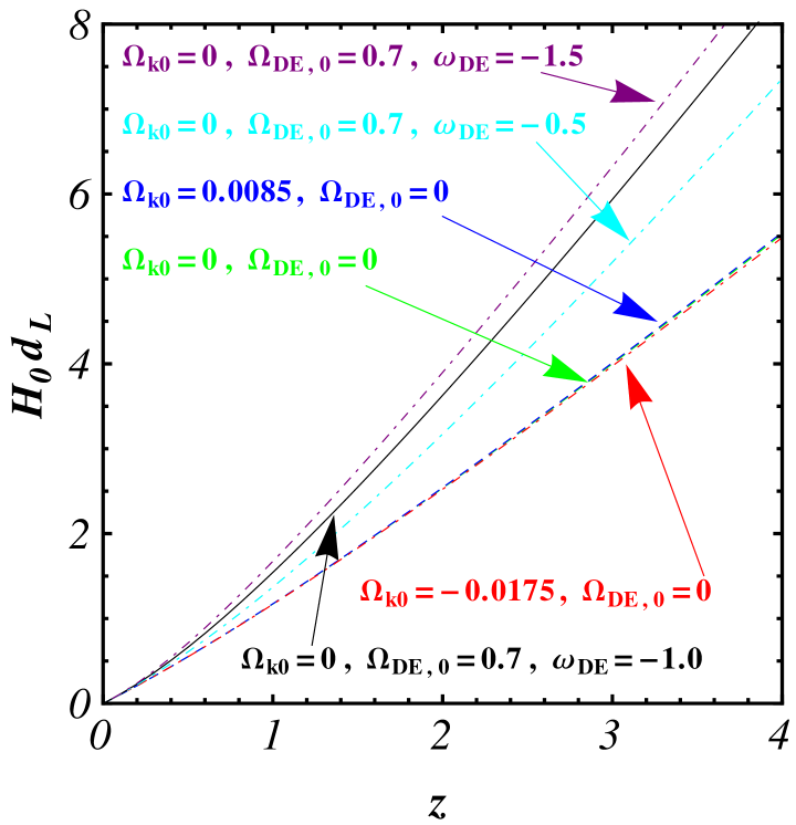
Figure 2: The luminosity distance $d_{L}$ versus the redshift $z$ for six cases: (a) A flat Universe without dark energy (green dashed line, not very clearly visible since it lies between the blue dashed and red dot-dashed lines), (b) An open Universe ($\Omega_{k0}=0.0085$) without dark energy (blue dashed line), (c) A closed Universe ($\Omega_{k0}=-0.0175$) without dark energy (red dot-dashed line), (d) A flat Universe with cosmological constant with $\Omega_{DE,0}=0.7$ and $\omega_{DE}=-1$ (black solid line), (e) A flat Universe with dark energy whose equation of state parameter $\omega_{DE}=-0.5$ and density $\Omega_{DE}=0.7$ (cyan dot-dashed line), (f) A flat Universe with dark energy whose equation of state parameter $\omega_{DE}=-1.5$ and density $\Omega_{DE}=0.7$ (cyan dot-dashed line). The presence of dark energy leads to a larger luminosity distance relative to the case without it. In the open Universe the luminosity distance also gets larger than that in the flat Universe. Also, dark energy with smaller $\omega_{DE}$ and larger $\Omega_{DE}$ leads to a larger luminosity distance.

This plot shows that incorporating dark energy (black solid line) leads to a larger luminosity distance relative to the case when dark energy is neglected (red, green and blue plots). Also, it is clear from Fig. (2) that for smaller $\omega_{DE}$ and for larger $\Omega_{DE}$ the luminosity distance becomes larger significant. Here a point to note is that an open Universe $\Omega_{k0}>0$ ($k<0$) has a larger luminosity distance than a flat Einstein-de Sitter Universe. But since the curvature of the Universe is constrained very close to flat⁹⁰ ($-0.0175<\Omega_{k0}<0.0085$) from WMAP 5 year data, it is very difficult to increase the luminosity distance in an open Universe without dark energy as compared to a flat Universe with dark energy.

We now consider some examples of the observational apparent luminosity verses redshift for high redshift Type Ia supernovae ($0.2<z<0.8$),^{144, 127} , to illustrate how luminosity distance is determined.

In Table (1) we consider the apparent magnitude data in low redshift range. For low $z$ the luminosity distance is $d_{L}\approx{z}/{H_{0}}$ from Eq. (34). Considering a Hubble constant, $H_{0}=70$ km s^-1 Mpc^-1 leads to the absolute magnitude of both SNeIa being approximately $-19$ as discussed above.

[b]

Table 1: Illustrate SNeIa Apparent Magnitude Data at Low $z$

Name of SN	Redshift	Apparent	Luminosity	Absolute
		Magnitude	Distancea	Magnitudeb
	$z$	$m$	$H_{0}d_{L}$	$M$
1990O	0.03	16.26	0.03	-19.28
1992bg	0.036	16.66	0.036	-19.29

• Here redshift $z\ll 1$ so $d_{L}H_{0}=z$ (considering $c=1$).

• Absolute magnitude is computed from Eq. (37) in the small $z$ approximation thus $M=m-5\ \mathrm{log_{10}}\left(\frac{z}{10\ \mathrm{pc}\ H_{0}}\right)$. Here we assume $H_{0}=70$ km s^-1 Mpc^-1.

Let’s consider 2 high redshift SNeIa data points from Perlmutter et al.¹²⁷ shown in the Table (2).

[b]

Table 2: Illustrate SNeIa Apparent Magnitude Data at High $z$¹²⁷

Name of SN	Redshift	Apparent	Luminosity
		Magnitude	Distancea
	$z$	$m$	$H_{0}d_{L}$
1997R	0.657	23.83	0.920
1995ck	0.656	23.57	0.817

• To calculate the luminosity distance, we assumed an absolute magnitude $M=-19.15$. Note that in this case the small redshift approximation is not valid hence we use Eq. (29) for the computation of the luminosity distance.

Here, luminosity distance is calculated by assuming absolute magnitude $M=-19.15$. Also for large redshift we cannot use approximate luminosity distance ${z}/{H_{0}}$, instead we use the more general equation (29).

Let’s consider a flat Universe ($\Omega_{k0}=0$) with dark energy whose equation of state parameter is $\omega_{DE}\approx-1$ (i.e. a cosmological constant). Then from Eq. (278):

$$E(z)=\sqrt{\Omega_{m0}(1+z)^{3}+\Omega_{DE,0}}.$$ (34)

In this case the luminosity distance is given by

$$d_{L}(z)=\frac{(1+z)}{H_{0}}{{{\int}}}\limits^{z}_{0}\frac{dz^{\prime}}{\Big{[}\Omega_{m0}(1+z^{\prime})^{3}+\Omega_{DE,0}\Big{]}^{1/2}},$$ (35)

which needs to be evaluated numerically. In order to satisfy observational data $H_{0}d_{L}(z=0.657)=0.920$ for $1997$R we require that $\Omega_{DE,0}=0.7$. Similarly we get $\Omega_{DE,0}=0.38$ from the $1995$ck data. Both indicate the requirement of dark energy to make an agreement between the theoretical predictions and the observations.

Of course, two data points are not enough to conclude that of dark energy is required and that the current cosmological expansion is accelerating. Using 570 SNeIa data points,¹⁶⁸ Farooq and Ratra,⁶⁰ put constraints on $\omega_{DE}$ (considering a time-independent equation of state parameter) which came out to be $-0.97<\omega_{DE}<-1.03$ ($1\sigma$ interval) and the $1\sigma$ constraints on non-relativistic matter density was found to be $0.24<\Omega_{m0}<0.34$.

All this discussion leads to the conclusion that dark energy can provide a good fit to the observational data.

3 Baryonic Acoustic Oscillation (BAO) Measurements

Before the recombination epoch, baryons are tightly coupled to photons so sound waves oscillations will be imprinted in the baryon perturbations as well in CMB temperature anisotropies. Eisenstein $et\ al.$ ⁵⁷ were the first, in 2005, to report on baryon acoustic oscillation peak in the large-scale correlation function measured from a spectroscopic sample of 46,748 luminous red galaxies observed by the Sloan Digital Sky Survey (SDSS). The detection of BAOs provides another independent technique for probing dark energy.

The sound horizon at which baryons were released from the Compton drag of photons determines the location of the baryon acoustic oscillation peak length scale. This epoch, called the drag epoch, occurs at the redshift $z_{d}$ and the length scale is

$$r_{s}(z_{d})=\int\limits^{\eta_{\mathrm{drag}}}_{0}c_{s}(\eta)\ \mathrm{d}\eta,$$ (36)

where $c_{s}$ is the speed of sound and $\eta$ is conformal time. We emphasize that the drag epoch is not the same that as recombination epoch at which the photons were release from the electrons.

Using the fitting formula of $z_{d}$ by Eisenstein and Hu,⁵⁶ $z_{d}$ and $r_{s}(z_{d})$ are constrained (from WMAP 5 year data⁹⁰) to be $z_{d}\approx 1020.5\pm 1.6$ and $r_{s}(z_{d})=153.3\pm 2.0$ Mpc.

The observed angular and redshift distributions of galaxies can be characterized by a power spectrum $P(k_{\bot},k_{\|})$ in redshift $z$ space. Here $k_{\bot}$ and $k_{\|}$ are the wave numbers parallel and perpendicular to the line of sight respectively. In principle, we can measure the following two ratios^{3, 160}

$$\theta_{s}(z)=\frac{r_{s}(z_{d})}{(1+z)d_{A}(z)},\hskip 28.45274pt\delta z_{s}(z)=\frac{r_{s}(z_{d})H(z)}{c},$$ (37)

where $c$ is the speed of light reintroduced for clarity. Here $\theta_{s}(z)$ characterizes the angle distribution orthogonal to the line of sight, while $\delta z_{s}$ corresponds to the oscillation along the line of sight.

Most current BAO observations cannot measure both $\theta_{s}(z)$ and $\delta z_{s}(z)$ independently, but form a spherically averaged spectrum, it is possible to determine a combined distance scale ratio given as⁵⁷

$$\left[\theta_{s}^{2}(z)\delta z_{s}(z)\right]^{1/3}=\frac{r_{s}(z_{d})}{\Big{[}(1+z)^{2}d_{A}^{2}(z)c/H(z)\Big{]}^{1/3}},$$ (38)

or an effective distance ratio

$$D_{V}(z)=\left[(1+z)^{2}d_{A}^{2}(z)\frac{c}{H(z)}\right]^{1/3}.$$ (39)

In 2005, Eisenstein et al.⁵⁷ obtained $D_{V}(z)=1370\pm 64$ Mpc at $z=0.68$.

In 2007, Percival et al.,¹²⁴ measured the effective distance ratio defined by

$$r_{\mathrm{BAO}}(z)=\frac{r_{s}(z_{d})}{D_{V}(z)},$$ (40)

at two different redshifts, $r_{\mathrm{BAO}}(z=0.2)=0.1980\pm 0.0058$ and $r_{\mathrm{BAO}}(z=0.35)=0.1094\pm 0.0033$. This is based on data from the 2-degree Field (2-dF) Galaxy redshift survey.

Figure 3: $1\sigma$, $2\sigma$, and $3\sigma$ constraint contours leaving $\omega_{DE}$ as free parameter. The dashed horizontal lines at $\omega_{DE}=-1$ correspond to spatially-flat $\Lambda$CDM models and the curved dotted lines demarcate zero-acceleration models. The constraints contours are obtained using the 6 BAO data given in Table (1) the plot is taken from Farooq et al.⁶⁰ The method to obtain these contours is explained in Chapter (4). The solid dot is best fit point located at $(\Omega_{m0},\omega_{X})=(0.27,-1.21)$. The corresponding $\chi^{2}_{\mathrm{min}}=5.5$.

In 2010, Percival et al.¹²³ used SDSS data to determine $r_{\mathrm{BAO}}(z=0.2)=0.1905\pm 0.0061$ and $r_{\mathrm{BAO}}(z=0.35)=0.1097\pm 0.0036$. In 2011, using 6dF Galaxy Survey (6dFGS) measurements, Beutler et al.¹⁵ found $r_{\mathrm{BAO}}(z=0.106)=0.3360\pm 0.015$.

Then in 2011, Black et al.¹⁹ considered the acoustic parameter introduced by Eisenstein et al.,⁵⁷

$$A(z)\equiv\frac{100D_{V}(z)\sqrt{\Omega_{m}h^{2}}}{cz},$$ (41)

and based on the data from WiggleZ Dark Energy Survey found $A(z)$ at three different redshifts [given in the Table (3) of Blake ¹⁹]: $A(z=0.44)=0.474\pm 0.034$, $A(z=0.6)=0.442\pm 0.020$, and $A(z=0.44)=0.424\pm 0.021$. These are summarized in Table (1).

Using the data from Percival et al.¹²³, Blake et al.¹⁹, and Beutler et al.¹⁵, Farooq et al.⁶⁰ found the constraints on the $\omega_{DE}$ shown in the Fig. (3). Figure (3) shows the constraints obtained using BAO observational data for the general but time independent equation of state parameters $\omega_{DE}$ for dark energy, also provides evidence for a current epoch cosmological expansion that is accelerating, and thus support for the existence of dark energy.

2 Spatially-Flat $\Lambda$CDM Model (Standard Cosmological Model)

Most currently available cosmological data are largely consistent with a spatially-flat, cosmological constant ($\Lambda$) dominated model with $\Omega_{\Lambda}\approx 0.7$ and with the rest of the energy being non-relativistic (baryonic and cold dark) matter $\Omega_{m0}\approx 0.3$, where baryonic matter makes up only 5% of the Universe ($\Omega_{b}\approx 0.05$). The cosmological constant can be considered to be an ideal fluid with equation-of-state parameter $\omega_{\Lambda}=-1$, hence from Eq. (139) its energy density does not change with time ($\rho_{\Lambda}=\rho_{\Lambda 0}\ \ \forall$ t). This spatially-flat $\Lambda$CDM model¹¹⁹ is often referred to as the “standard model”. In this model the Hubble parameter, from the Friedmann equation (278), obeys

$$H(z,H_{0},\textbf{p}) = H_{0}\left[\Omega_{m0}(1+z)^{3}+(1-\Omega_{m0})\right]^{1/2}.$$ (42)

Here we have neglected the radiation term and set $1-\Omega_{0}=0$ for this spatially-flat case so $\Omega_{\Lambda}=1-\Omega_{m0}$. This is one parameter model, with $\textbf{p}=\Omega_{m0}$ being the parameter characterize the model, and $H_{0}$ is the current value of Hubble parameter.

Although the spatially-flat $\Lambda$CDM model is a reasonable fit to most observations, the data is not yet precise enough to rule out other models of dark energy.

3 $\Lambda$CDM with Non-Zero Curvature

This is a generalization of the standard model of cosmology within the frame work of general relatively. Here we also consider spatial curvature $k$ with present value density parameter denoted by $\Omega_{k0}$, as defined in Eq. (277). In this case the Friedmann equation (278) for the evolution of the Hubble parameter is

$$H(z)=H_{0}\left[\Omega_{m0}(1+z)^{3}+\Omega_{\Lambda}+(1-\Omega_{m0}-\Omega_{\Lambda})(1+z)^{2}\right]^{1/2},$$ (43)

where, since $\Omega_{m0}+\Omega_{k0}+\Omega_{\Lambda}=1$, we have replaced $\Omega_{k0}$ by $1-\Omega_{m0}-\Omega_{\Lambda}$ and this is with parameters $\textbf{p}=(\Omega_{m0},\Omega_{\Lambda})$.

1 No Big Bang Region in the ${\Lambda}$CDM Model

Returning to the general case of models with a combination of energy in the vacuum $(\Lambda)$ and normal components, we have to distinguish three cases. For models that start from a big bang (in which case radiation dominates at early times), the Universe will either recollapse or expand forever. The latter outcome becomes more likely for low densities of matter and radiation and high vacuum density. It is however also possible to have models in which there is no big bang: the Universe was collapsing in the distant past, but was slowed by the repulsion of a positive $\Lambda$ term and underwent a “bounce” to reach its present state of expansion.

We can compute an analytical formula $\Omega_{\Lambda}(\Omega_{m0})$ which separates models with a big bang from those without a big bang. It is given as follows:

$$\Omega_{\Lambda}(\Omega_{m0})\geq\left\{\begin{array}[]{lc}4\ \Omega_{m0}\ \mathrm{cosh^{3}}\left[\frac{1}{3}\mathrm{cosh^{-1}\left(\frac{1-\Omega_{m0}}{\Omega_{m0}}\right)}\right],&0\leq\Omega_{m0}\leq\frac{1}{2}\\ &\\ 4\ \Omega_{m0}\ \mathrm{cos^{3}}\left[\frac{1}{3}\mathrm{cos^{-1}\left(\frac{1-\Omega_{m0}}{\Omega_{m0}}\right)}\right],&\frac{1}{2}\leq\Omega_{m0}\\ \end{array}.\right.\vspace{1cm}$$ (44)

The derivation follows

The Friedman equations, which are derived from Einstein’s theory of general relativity in Chapter (), are

$$\left(\frac{\dot{a}}{a}\right)^{2}=\frac{8\pi G}{3}\rho+\frac{\Lambda}{3}-\frac{k}{a^{2}},$$ (45)

$$\frac{\ddot{a}}{a}=-\frac{4\pi G}{3}\left(\rho+3p\right)+\frac{\Lambda}{3}.$$ (46)

Equation (45) can be rewritten as:

$$\frac{k}{a^{2}} = H^{2}(t)\left[\Omega_{m}(t)-1\right]+\frac{\Lambda}{3}=H^{2}(t)\left[\Omega_{m}(t)-1+\frac{\Lambda}{3H^{2}(t)}\right].$$ (47)

At the present time $a=a_{0}=1$ and $H=H_{0}$, hence the above equation takes the form:

$$k=H_{0}^{2}\left[\Omega_{m0}-1+\frac{\Lambda}{3H_{0}^{2}}\right].$$ (48)

A Universe with a large value of $\Omega_{\Lambda}\equiv{\Lambda}/{3H^{2}_{0}}$ (say $\Omega_{\Lambda_{c}}$), loses the big bang in the beginning and we instead obtain an Eddington-Lemaître (EL) model, asymptotic to Einstein’s static model in the infinite past.⁶³ For $\Omega_{\Lambda}\geq\Omega_{\Lambda_{c}}$, we obtain models that collapse from infinity, reach a minimum value $a(t)$ and then expand again. These Universes are sometimes called “catenary Universes”. Here it is important to note that the catenary Universes, like the re-collapsing models with large negative $\Lambda$, are time symmetric about their extrema in $a$, where $\dot{a}(t)=0$. This is expected, because the Friedman Eq. (45) is manifestly time symmetric: if $a(t)$ is a solution, $a(-t)$ is also.

It is of interest to obtain an analytical expression for the critical value $\Omega_{\Lambda}$ at which the Universe no longer starts from a big bang. To do this we note that the critical (EL) model is asymptotic to a static Einstein model in the infinite past, so that in that state it must satisfy $\dot{a}=\ddot{a}=p=0$, then $\Omega_{\Lambda}=\Omega_{\Lambda_{c}}$, $\Lambda=\Lambda_{c}$ and $a=a_{c}$ with these conditions, using Eqs. (45) and (46), we can require:

$$\left(\frac{\dot{a}}{a}\right)^{2}_{c}+2\left(\frac{\ddot{a}}{a}\right)_{c} = 0,$$ (49)

$$\Rightarrow\cancel{\frac{8\pi G}{3}\rho_{c}}+\frac{\Lambda_{c}}{3}-\frac{k}{a^{2}_{c}}-\cancel{\frac{8\pi G}{3}\rho_{c}}+\frac{2\Lambda_{c}}{3}=0,$$ (50)

this can be simplified as:

$$\Lambda_{c}=\frac{k}{a^{2}_{c}}.$$ (51)

From Eq. (46) at these conditions leads to:

$$\Lambda_{c} = 4\pi G\rho_{c}(t)=\frac{3}{2}\left(\frac{8\pi G}{3}\rho_{0}\right)\frac{1}{a^{3}_{c}}.$$ (52)

Defining,

$$\mathcal{C}\equiv\frac{8\pi G}{3}\rho_{0}=H^{2}_{0}\Omega_{m0},$$ (53)

we can write Eq. (52) as

$$\Lambda_{c}=\frac{3}{2}\ \mathcal{C}a^{-3}_{c}.$$ (54)

Comparing Eqs. (51) and (54) we have

$$\Lambda_{c}=k\ a^{-2}_{c}=\frac{3}{2}\ \mathcal{C}a^{-3}_{c}.$$ (55)

Solving Eq. (55) for $a_{c}$ we find

$$a_{c}=\frac{3\mathcal{C}}{2k}.$$ (56)

Plugging the value of $a_{c}$ back in Eq. (54) and simplifying,

$$\Lambda_{c}=\frac{4}{9}\mathcal{C}^{-2}k^{3},$$ (57)

using the definition of $\mathcal{C}$ from Eq. (53) leads to

$$\Lambda_{c}=\frac{4}{9}\left(\Omega_{m0}H^{2}_{0}\right)^{-2}k^{3},$$ (58)

and dividing both sides by $\left(\Omega_{m0}H^{2}_{0}\right)$ gives

$$\frac{\Lambda_{c}}{\left(\Omega_{m0}H^{2}_{0}\right)}=\frac{4}{9}\left(\frac{k}{\Omega_{m0}H^{2}_{0}}\right)^{3},$$ (59)

Plugging the value of $k$ from Eq. (48) in to Eq. (59) results in:

$$\frac{\Lambda_{c}}{\left(\Omega_{m0}H^{2}_{0}\right)}=\frac{4}{9}\left[\frac{\cancel{H_{0}^{2}}\left(\Omega_{m0}-1+\frac{\Lambda}{3H_{0}^{2}}\right)}{\Omega_{m0}\cancel{H^{2}_{0}}}\right]^{3}.$$ (60)

and simplifying this leads to

$$\left(\frac{\Lambda_{c}}{12\Omega_{m0}H^{2}_{0}}\right)^{1/3}=\frac{1}{3}\left[\frac{\Omega_{m0}-1}{\Omega_{m0}}+4\ \frac{\Lambda_{c}}{12\Omega_{m0}H^{2}_{0}}\right].$$ (61)

Defining

$$x\equiv\left(\frac{\Lambda_{c}}{12\Omega_{m0}H^{2}_{0}}\right)^{1/3},$$ (62)

the above equation takes the from:

$$x^{3}-\frac{3}{4}x+\frac{1}{4}\left(\frac{\Omega_{m0}-1}{\Omega_{m0}}\right)=0.$$ (63)

This is a standard cubic equation whose, solutions are discussed in Appendix (11). Using Eqs. (10) and (14) the value of $x$ is

$$x=\left\{\begin{array}[]{lc}\mathrm{cosh}\left[\frac{1}{3}\mathrm{cosh^{-1}\left(\frac{1-\Omega_{m0}}{\Omega_{m0}}\right)}\right],&0\leq\Omega_{m0}\leq\frac{1}{2}\\ &\\ \mathrm{cos}\left[\frac{1}{3}\mathrm{cos^{-1}\left(\frac{1-\Omega_{m0}}{\Omega_{m0}}\right)}\right],&\frac{1}{2}\leq\Omega_{m0}\\ \end{array}.\right.$$ (64)

We can write these no big bang conditions in terms of $\Omega_{\Lambda_{c}}$, using Eq. (62), as

$$\Omega_{\Lambda}(\Omega_{m0})\geq\Omega_{\Lambda_{c}}=\left\{\begin{array}[]{lc}4\ \Omega_{m0}\ \mathrm{cosh^{3}}\left[\frac{1}{3}\mathrm{cosh^{-1}\left(\frac{1-\Omega_{m0}}{\Omega_{m0}}\right)}\right],&0\leq\Omega_{m0}\leq\frac{1}{2}\\ &\\ 4\ \Omega_{m0}\ \mathrm{cos^{3}}\left[\frac{1}{3}\mathrm{cos^{-1}\left(\frac{1-\Omega_{m0}}{\Omega_{m0}}\right)}\right],&\frac{1}{2}\leq\Omega_{m0}\\ \end{array}.\right.$$ (65)

These are plotted (in red and blue) in Fig. (4)

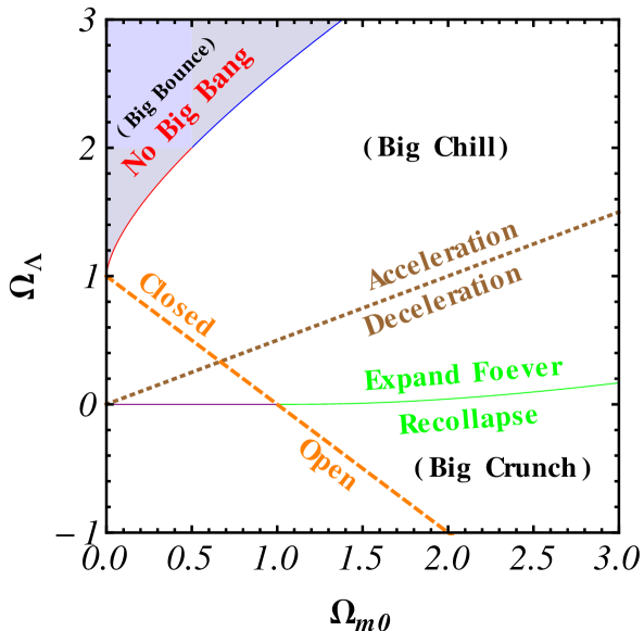
Figure 4: Different regions of $\Omega_{m0}-\Omega_{\Lambda}$ plane of the two-parameter $\Lambda$CDM model represent different evolutionary cosmological histories. The brown dotted line [which is the plot of Eq. (84)] separates accelerating and decelerating Universes. The Orange dashed line [which is the plot of Eq. (81)] demarcates closed and open Universes. The gray portion of the parameter plane above the red and the blue curves at the left top [the curves are the plot of Eq. (65)] represent Universes with no big bang back in time. These Universes are called “Big Bounce” Universes because they started contracting from a non zero size, reached a minimum size, and then start expanding. The purple line and the green curve [which are the plot of Eq. (80)] distinguish between the Universes that will expand forever those that will recollapse. Universes that will recollapse lie below the purple-green curve “Big Crunch”, while Universe above the purple-green-line are in the “Big Chill”, in the region labeled.

2 Condition for Recollapse in the ${\Lambda}$CDM Model

As $a\rightarrow 0$, in the past space curvature and vacuum energy is negligible and the $\Lambda$CDM model will behave as an Einstein-de Sitter model until the radiation become important. As $a\rightarrow\infty$, in the future space curvature and the matter energy becomes negligible and the $\Lambda$CDM model will asymptote to the de Sitter model, unless the scale factor never reaches $\infty$ because the $\Lambda$CDM model Universes re-collapses at a finite time. Two possibilities for the evolution of $\Lambda$CDM model are:

• $\Omega_{\Lambda}<0$: always decelerates and recollapses [as explained in Section (1)] as vacuum energy is always going to dominate.

• $\Omega_{\Lambda}\geq 0$: recollapse is possible if $\Omega_{m0}$ is large enough to halt the expansion before $\Omega_{\Lambda}$ dominates.

To determine the dividing line between perpetual expansion and eventual recollapse, note that collapse requires that the Hubble parameter to pass through $0$ as it changes from positive to negative, so at turn around

$$H^{2}(t_{t})=0=\frac{8\pi G}{3}\ \left[\rho_{m0}\ a^{-3}_{t}+\rho_{\Lambda,0}+\rho_{k0}\ a^{-2}_{t}\right],$$ (66)

where $t_{t}$ and $a_{t}$ is the time and the scalar factor at turn around. Dividing by $H^{2}_{0}$ and using $\Omega_{k0}=1-\Omega_{m0}-\Omega_{\Lambda}$, and rearranging, we obtain

$$\Omega_{\Lambda}\ a^{3}_{t}+\left(1-\Omega_{m0}-\Omega_{\Lambda}\right)\ a^{2}_{t}+\Omega_{m0}=0.$$ (67)

But what we really care about is not really $a_{t}$, but the range of $\Omega_{m0}$ and $\Omega_{\Lambda}$ for which there is at least one real solution of Eq. (67).

Let’s find the condition for Eq. (67) to have one positive real solution. Equation (67) can be written as

$$a^{3}_{t}+\frac{1-\Omega_{m0}-\Omega_{\Lambda}}{\Omega_{\Lambda}}\ a^{2}_{t}+\frac{\Omega_{m0}}{\Omega_{\Lambda}}=0.$$ (68)

Comparing this with Eq. (5), which is standard from of cubic equation, we define the parameters

$$x=a_{t},\hskip 28.45274ptP=\frac{1-\Omega_{m0}-\Omega_{\Lambda}}{\Omega_{\Lambda}},\hskip 28.45274ptQ=\frac{\Omega_{m0}}{\Omega_{\Lambda}}.$$ (69)

Consider the cubic polynomial

$$y(x)=x^{3}+Px+Q.$$ (70)

If $Q<0$, this means that the plot of $y(x)$ will have the negative $y$-intercept and since the co-efficient of $x^{3}$ is positive the corresponding cubic equation $y(x)=0$ will have at least one positive root.

If $Q>0$ (then we need $P<0$ so that the curve will have negative slope when it intersects the $y$-axis; this means $\Omega_{m0}\geq 1$) then the cubic equation will have at least one negative real solution (from the same argument as above). In this case to make sure that the cubic equation will have at least are positive solution as well, we have to find an $x_{0}>0$ such that $\frac{dy}{dx}\big{|}_{x_{0}}=0$ and $y(x_{0})=0$. Thus:

$$\frac{dy}{dx} = 3x^{2}+P=0.$$

$$\Rightarrow x_{0} = +\sqrt{\frac{-P}{3}},\hskip 28.45274pt\left(\mathrm{we\ will\ consider\ only\ positive\ root}\right)$$ (71)

and $y(x_{0})=0$ leads to:

$$\Rightarrow\left(-\frac{P}{3}\right)^{3/2}+P\left(-\frac{P}{3}\right)^{1/2}+Q=0,$$ (72)

$$\Rightarrow-4P^{3}=27Q^{2}.$$ (73)

Substituting the values of $P$ and $Q$ from Eq. (69) we find:

$$\left(1-\Omega_{m0}-\Omega_{\Lambda}\right)^{3}=-\frac{27}{4}\Omega_{m0}^{2}\Omega_{\Lambda}.$$ (74)

Under the given condition $\Omega_{m0}\geq 1$, we can write:

$$\left(\frac{1-\Omega_{m0}-\Omega_{\Lambda}}{3\Omega_{m0}}\right)^{3}=-\frac{\Omega_{\Lambda}}{4\Omega_{m0}}.$$ (75)

$$\Rightarrow\frac{1-\Omega_{m0}}{3\Omega_{m0}}-\frac{4}{3}\left(\frac{\Omega_{\Lambda}}{4\Omega_{m0}}\right)=-\left(\frac{\Omega_{\Lambda}}{4\Omega_{m0}}\right)^{1/3}.$$ (76)

Defining

$$x\equiv\frac{4}{3}\left(\frac{\Omega_{\Lambda}}{4\Omega_{m0}}\right)^{1/3},$$ (77)

we can rewrite Eq. (76) as

$$x^{3}-\frac{3}{4}x-\frac{1}{4}\left(\frac{1-\Omega_{m0}}{\Omega_{m0}}\right)=0.$$ (78)

Using the solution of standard cubic equation from Appendix (11), the solution of this equation is

$$x=\mathrm{cos}\left[\frac{1}{3}\mathrm{cos^{-1}}\left(\frac{1-\Omega_{m0}}{\Omega_{m0}}\right)+\frac{4\pi}{3}\right],$$ (79)

and in terms of the parameters of the $\Lambda$CDM model we have

$$\Omega_{\Lambda}=4\ \Omega_{m0}\ \mathrm{cos^{3}}\left[\frac{1}{3}\mathrm{cos^{-1}}\left(\frac{1-\Omega_{m0}}{\Omega_{m0}}\right)+\frac{4\pi}{3}\right].$$ (80)

The plot of this equation is shown (green curve) in Fig. (4)

3 Flat ${\Lambda}$CDM and the Zero Acceleration Line for General ${\Lambda}$CDM

Since $\Omega_{k0}=1-\Omega_{m0}-\Omega_{\Lambda}$, for the flat case when $\Omega_{k0}=0$ we have

$$\Omega_{\Lambda}=1-\Omega_{m0}.$$ (81)

The plot of this equation is shown (orange dashed line) in Fig. (4).

To derive zero acceleration line, consider the acceleration equation with only non-relativistic matter and a cosmological constant

$$\frac{\ddot{a}}{a}=-\frac{4\pi G}{3}\Big{[}\rho_{m}\left(1+3\omega_{m}\right)+\rho_{\Lambda}\left(1+3\omega_{\Lambda}\right)\Big{]}.$$ (82)

But as discussed before $\omega_{m}=0$, and $\omega_{\Lambda}=-1$, hence:

$$\frac{\ddot{a}}{a}=-\frac{4\pi G}{3}\left[\rho_{m}-2\rho_{\Lambda}\right]=-2H_{0}^{2}\left[\frac{\Omega_{m0}}{a^{3}}-2\Omega_{\Lambda}\right].$$ (83)

For the zero acceleration today we set $\ddot{a}=0$, and $a=a_{0}=1$, which gives

$$\hskip 56.9055pt\Omega_{\Lambda}=\frac{1}{2}\Omega_{m0}.\hskip 56.9055pt\left[\mathrm{since}\ H_{0}\neq 0\right]$$ (84)

The plot of this equation is shown (brown dotted line) in Fig. (4)

4 Potential Problems with $\Lambda$CDM

The $\Lambda$CDM cosmological model is a well defined, simple, classically consistent, and predictive model which is largely consistent with most of the current cosmological observations. Despite of these successes there are some theoretical and observational reasons to go beyond the standard cosmological model.

1 Theoretical Puzzles

Cosmological Constant Puzzle

The cosmological constant is difficult to motivate from fundamental physics. Since the cosmological constant is equivalent to a constant energy density, it likely receives contributions from many sources. A problematic source is zero point vacuum energy. For example, the standard quantum mechanical harmonic oscillator (or any other bound system) has a energy proportional to the frequency, given by $\hbar\omega/2$ even in the absence of excitations. The zero point energy of some field of mass $m$ with momentum $k$ and frequency $\omega$ is given by $E=\hbar\omega/2=\hbar\sqrt{k^{2}+m^{2}}/2$. Summing over the zero point energies of this field up to the cut off scale $k_{\mathrm{max}}$ we obtain for the vacuum energy density

$$\rho_{\mathrm{vac}}={{\int}}\limits^{k_{\mathrm{max}}}_{0}\frac{\hbar}{2}\sqrt{k^{2}+m^{2}}\frac{d^{3}k}{(2\pi)^{3}}.$$ (85)

Since the integral is dominated by short wavelength modes with $k\gg m$, we find

$$\rho_{\mathrm{vac}}\approx{{\int}}\limits^{k_{\mathrm{max}}}_{0}\frac{\hbar}{2}k\frac{4\pi k^{2}dk}{(2\pi)^{3}}=\frac{k_{\mathrm{max}}^{4}}{16\pi^{2}}.$$ (86)

Quantum field theory is expected to break down at the Planck scale of around $10^{19}$ GeV. If we use this as the cutoff limit in Eq. (86), we get a huge number $\rho_{\mathrm{vac}}\approx 10^{74}\ \mathrm{GeV^{4}}$ that exceeds the observed dark energy density ($\rho_{DE,0}\approx 10^{-44}\ \mathrm{GeV^{4}}$)¹⁸³ by 120 orders of magnitude.¹⁷³

In a super-symmetric model every boson has a fermion of equal mass as a super-symmetric partner and the vacuum energies of these partners cancel. Super-symmetry (SUSY), if existent, is believed to be broken at an energy of roughly 1 TeV or so. If we cut off the upper integration limit in Eq. (86) at the energy of SUSY breaking we will still get a difference of around 46 orders of magnitude. This discrepancy between the small measured value of the cosmological constant and the much larger theoretically “expected” values of vacuum energy is known as the “smallness” problem.¹⁸³

One potential explanation of the smallness problem is based on anthropic arguments. In string theory, multiple vacuum states with all possible values of vacuum energy are possible. Different causally disconnected patches of the Universe spontaneously choose vacuum states that are independent of each other. If the Universe is infinite there will always be parts of it that have a given value, no matter how unlikely, of the vacuum energy and we just happen to live in one of those regions with a very small value of vacuum energy density.^{166, 22}

Coincidence Puzzle

Another interesting fact that is difficult to explain in the $\Lambda$CDM model is that current energy density of non-relativistic matter $\rho_{m0}$ and that of the cosmological constant $\rho_{\Lambda}$ have a comparable magnitudes, but their relative scaling $\rho_{\Lambda}/\rho_{m}\propto a^{3}$, implies that $\Lambda$ was completely negligible in the cosmological past and will absolutely dominate in the future. Summarizing, the radiation energy density redshift as $a^{-4}$ hence the Universe was dominated by radiation at very early times, the Universe then became dominated by non-relativistic (baryonic and cold dark) matter (since $\rho_{m}\propto a^{-3}$), and very recently⁶² the Universe became $\Lambda$ dominated. In the future dark energy will be the only component driving cosmic expansion. If we consider cosmological constant to be set as an initial condition in the very early Universe (when the non-relativistic energy density was very high as compared to the current value of non-relativistic energy density), it seems very unlikely that $\Lambda$ should have a value comparable to that of matter at the present cosmological epoch, when galaxies and other large scale structures have formed. If the cosmological constant was a couple of orders of magnitude higher than what is now observed, the Universe would be empty of large-scale-structure. But if it were just a couple of orders of magnitude smaller $\Lambda$ would be hardly detectable.

The lack of an explanation for why dark energy has the same order as non-relativistic matter density at the present epoch is known as the coincidence problem. One potential resolution of this is again the anthropic principle.¹⁶⁶

2 Potential Observational Problems¹²⁵

There are a number of observations that are not consistent with the standard $\Lambda$CDM model of cosmology. It is not yet clear if all of these measurements are definitive. More observational work is needed to settle the issue, some are given here:

Large-Scale Velocity Flows

$\Lambda$CDM predicts a significantly smaller amplitude and scale of velocity flows than what some observations seems to indicate.

Brightness of Type Ia Supernovae (SNIa)

$\Lambda$CDM predicts fainter SNIa at high redshift then some that are observed.

Emptiness of Voids

$\Lambda$CDM predicts more dwarf or irregular galaxies in the voids than are observed.

Profiles of Cluster Haloes

$\Lambda$CDM predicts shallow, low concentration and less dense profiles, in contrast to the observations which indicate denser high concentration cluster haloes.

Profiles of Galaxy Haloes

$\Lambda$CDM predicts galaxy halo mass profiles with more dense cores and low outer density while lensing and dynamical observations indicate a central core of constant density and a flattish high dark-mass density outer profile.

Sizable Population of Disk Galaxies

$\Lambda$CDM predicts a smaller fraction of disk galaxies than is observed due to recent mergers that are expected to disrupt cold rotationally-supported disks.

It is interesting the most of the above-mentioned problems are apparently related to the dark matter. On the scale of clusters dark energy would play a significant role in the stability of some of these systems especially if the dark energy was coupled to dark matter through a new, non-gravitational force.

At the moment these discrepancies between observations and theoretical predictions do not carry great weight in the overall picture. The ΛCDM model is in general a good statistical fit to the combined data. These inconsistencies might go away, or could become more pressing, when new high-quality data become available.¹⁴⁹

5 XCDM Parameterization

The cosmological constant time-independent dark energy can be thought as a spatially homogeneous fluid with equation-of-state parameter $\omega_{\Lambda}=p_{\Lambda}/\rho_{\Lambda}=-1$, where $\rho_{\Lambda}$ and $p_{\Lambda}$ are the fluid energy density and pressure respectively. There is not yet strong observational evidence for the time-independence of dark energy. Hence, we can model dark energy as a spatially-homogeneous $X-$fluid with equation-of-state parameter $\omega_{X}=p_{X}/\rho_{X}<-1/3$, an arbitrary constant, where $\rho_{X}$ and $p_{X}$ are the energy density and pressure of the $X-$fluid respectively. When $\omega_{X}=-1$ the XCDM parametrization reduces to $\Lambda$CDM. In the more general, $\omega_{X}<-1/3$ case, the Hubble parameter evolves according to

$$H(z)=H_{0}\left[\Omega_{m0}(1+z)^{3}+\Omega_{X0}(1+z)^{3(1+\omega_{X})}+\Omega_{k0}(1+z)^{2}\right]^{1/2}.$$ (87)

Since $\Omega_{m0}+\Omega_{k0}+\Omega_{X0}=1$, hence we can write Eq. (87) explicitly in terms of the three free parameters as

$$H(z,H_{0},\textbf{p})=H_{0}\left[\Omega_{m0}(1+z)^{3}+(1-\Omega_{m0}-\Omega_{k0})(1+z)^{3(1+\omega_{X})}+\Omega_{k0}(1+z)^{2}\right]^{1/2}.$$ (88)

Here $\textbf{p}=(\Omega_{m0},\omega_{X},\Omega_{k0})$ are the parameters of this model. In the special case when we consider $\Omega_{k0}=0$ (flat space) then in this spatially-flat XCDM model $H(z)$ evolves as

$$H(z,H_{0},\textbf{p})=H_{0}\left[\Omega_{m0}(1+z)^{3}+(1-\Omega_{m0}-\Omega_{k0})(1+z)^{3(1+\omega_{X})}\right]^{1/2}.$$ (89)

In this case the flat XCDM model parameters are $\textbf{p}=(\Omega_{m0},\omega_{X})$.

1 No Big Bang Surface in the Parameter Space of the Non-Flat XCDM Parametrization

In the XCDM model, the Friedmann and acceleration equations are

$$\left(\frac{\dot{a}}{a}\right)^{2}=\frac{8\pi G}{3}\Big{[}\rho_{m0}a^{-3}+\rho_{X0}a^{-3(1+\omega_{X})}\Big{]}-\frac{k}{a^{2}},$$ (90)

$$\left(\frac{\ddot{a}}{a}\right)=-\frac{4\pi G}{3}\Big{[}\rho_{m0}a^{-3}+\rho_{X0}a^{-3(1+\omega_{X})}\left(1+3\omega_{X}\right)\Big{]}.$$ (91)

By applying the condition of no big bang as we did in Section (1), i.e., setting $\dot{a}=\ddot{a}=0$, to define $a=a_{c}$ we get,

$$\left(\frac{\dot{a}}{a}\right)^{2}\Bigg{|}_{c}+2\left(\frac{\ddot{a}}{a}\right)\Bigg{|}_{c}=-\frac{k}{a_{c}^{2}}-\frac{8\pi G}{3}\Big{[}3~{}\omega_{X}\rho_{X0}a^{-3(1+\omega_{X})}_{c}\Big{]}=0.$$ (92)

Solving for $a_{c}$ we find

$$a_{c}=\left[-\frac{8\pi G\omega_{X}\rho_{X0}}{k}\right]^{1/(1+3\omega_{X})}.$$ (93)

Using $\ddot{a}=0$ and $a=a_{c}$ in Eq. (91) leads to

$$\rho_{m0}=-\rho_{X0}\left(1+3\omega_{X}\right)a^{-3\omega_{X}}_{c}.$$ (94)

Since $\Omega_{m0}=\frac{8\pi G\rho_{m0}}{3H^{2}_{0}}$, $\Omega_{X0}=\frac{8\pi G\rho_{X0}}{3H^{2}_{0}}$, and $\Omega_{k0}=-\frac{k}{H^{2}_{0}}$, we can write this as

$$\Omega_{m0}=\Omega_{X0}\left(1+3\omega_{X}\right)\left[\frac{\Omega_{X0}}{\Omega_{m0}}\omega_{X}\right]^{-\frac{3\omega_{X}}{1+3\omega_{X}}},$$ (95)

and since $\Omega_{X0}=1-\Omega_{m0}-\Omega_{k0}$, the implicit condition for no big bang in the XCDM parametrization is

$$\Omega_{m0}+\left(1-\Omega_{m0}-\Omega_{k0}\right)\left(1+3\omega_{X}\right)\left[\frac{\left(1-\Omega_{m0}-\Omega_{k0}\right)}{\Omega_{m0}}\omega_{X}\right]^{-\frac{3\omega_{X}}{1+3\omega_{X}}}\leq 0.$$ (96)

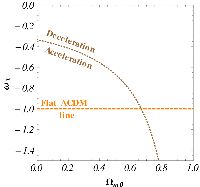
Figure 5: Different regions of $\Omega_{m0}-\omega_{X}$ plane represent different cosmological behavior in spatially-flat XCDM parametrization. The brown dotted line [which is the plot of Eq. (99)] separates accelerating from decelerating Universes, the orange dashed line [which is the plot of $\omega_{X}=-1$] shows the flat $\Lambda$CDM model.

2 Zero Acceleration Condition in the XCDM Parametrization

In the XCDM parametrization, the acceleration equation (91) in terms of density parameters, is

$$\frac{\ddot{a}}{a}=-\frac{1}{2}H_{0}^{2}\left[\frac{\Omega_{m0}}{a^{3}}+\frac{\Omega_{X0}}{a^{3(1+\omega_{X})}}\left(1+3\omega_{X}\right)\right].$$ (97)

For zero cosmological acceleration at the present time we set $a=a_{0}=1$, $\ddot{a}=0$ at present time we set $a=a_{0}=1$ in Eq. (97), and get

$$\Omega_{m0}+\Omega_{X0}\left(1+3\omega_{X}\right)=0.$$ (98)

Using $\Omega_{X0}=\left(1-\Omega_{m0}\right)$, in spatially-flat XCDM parametrization we can write the above equation as

$$\omega_{X}=\frac{1}{3\left(\Omega_{m0}-1\right)}.$$ (99)

6 Scalar Field Dark Energy Models

The cosmological constant is equivalent a fluid with constant equation-of-state parameter $\omega_{\Lambda}=-1$. In the XCDM parametrization the time-independent equation-of-state parameter $\omega_{X}=p_{X}/\rho_{X}$ can take any value ($<-1/3$ to make sure that the cosmic expansion accelerate which is now observationally established to high confidence). Observations which constrain the value of $\omega$ today to be close to that of a cosmological constant, actually tell us little about the time evolution of equation-of-state parameter of dark energy at early times. At very early times, it is widely thought that a scalar field drive inflation. Scalar fields naturally arise in particle physics and string theory and these might be candidates for dark energy. A wide variety of scalar-field dark energy models have been proposed (for a summery see Samushia¹⁴⁹).

The kind of scalar field dark energy model we will discuss is also known as Quintessence. It is described by a scalar field $\phi$ minimally coupled to gravity (but with particular potentials that leads to late time inflation-like accelerating cosmological expansion). The action of quintessence is

$$S=\int\sqrt{-g}\left[\frac{m^{2}_{p}}{16\pi}\left(\frac{1}{2}g^{\mu\nu}\partial_{\mu}\phi\partial_{\nu}\phi-V(\phi)-\mathcal{R}\right)+\mathcal{L}_{m}\right]d^{4}x,$$ (100)

where $m_{p}=1/\sqrt{G}$ is the Plank mass with $G$ being Newton’s gravitational constant, $\phi$ is a classical scalar field whose stress-energy tensor act like time-variable $\Lambda$, with potential energy density $V(\phi)$, $\mathcal{R}$ is the Ricci scalar curvature, and $\mathcal{L}_{m}$ is Lagrangian density for ordinary matter and radiation. The action Eq. (100) can be arrived at by writing down the Einstein-Hilbert action with the term $2\Lambda$ replaced by the Lagrangian density for scalar field $\phi$. In this sense one has a modification of General Relativity in which cosmological ‘constant’ can vary.

The Lagrangian density for the $\phi$ field is given as:

$$\mathcal{L}_{\phi}=\frac{m^{2}_{p}}{16\pi}\left[\frac{1}{2}g^{\mu\nu}\partial_{\mu}\phi\partial_{\nu}\phi-V(\phi)\right].$$ (101)

In a FLRW spacetime, the variation of this action with respect to $\phi$ gives equation of motion of $\phi$ field

$$\ddot{\phi}+3\left(\frac{\dot{a}}{a}\right)\dot{\phi}+\frac{dV}{d\phi}=0.$$ (102)

The energy-momentum tensor of the $\phi$ field is determined by varying $\mathcal{L}_{\phi}$ from Eq. (100)

$$T_{\mu\nu}=-2\frac{\delta\mathcal{L}_{\phi}}{\delta g^{\mu\nu}}+\mathcal{L}_{\phi}g_{\mu\nu},$$ (103)

and as derived in Appendix (10),

$$T_{\mu\nu}=\frac{m^{2}_{p}}{16\pi}\left[\partial_{\mu}\phi\partial_{\nu}\phi-g_{\mu\nu}\left(\frac{1}{2}g^{\alpha\beta}\partial_{\alpha}\phi\partial_{\beta}\phi+V(\phi)\right)\right].$$ (104)

The scalar field energy density

$$\rho_{\phi}=\frac{m^{2}_{p}}{16\pi}\left[\frac{1}{2}\dot{\phi}^{2}+V(\phi)\right],$$ (105)

and scalar field pressure

$$p_{\phi}=\frac{m^{2}_{p}}{16\pi}\left[\frac{1}{2}\dot{\phi}^{2}-V(\phi)\right].$$ (106)

Then the equation-of-state parameter for $\phi$ field is

$$\omega_{\phi}=\frac{p_{\phi}}{\rho_{\phi}}=\frac{\frac{1}{2}\dot{\phi}^{2}-V(\phi)}{\frac{1}{2}\dot{\phi}^{2}+V(\phi)},$$ (107)

Using Eq. (235) and (246), and the above expressions for the scalar field energy density and pressure, we get the Friedmann equation

$$H^{2} = \frac{1}{6}\left[\frac{1}{2}\dot{\phi}^{2}+V(\phi)\right],$$ (108)

$$\frac{\ddot{a}}{a} = -\frac{1}{6}\left[\dot{\phi}^{2}+V(\phi)\right].$$ (109)

1 Ratra-Peebles Scalar Field Model

In 1988 Ratra and Peebles proposed a scalar field model¹²¹ known as $\phi$CDM and in order to alleviate two problems of the standard $\Lambda$CDM model of cosmology. These are the coincidence and energy scale problems (discussed in Sec. (4). The energy problem is that the very small spatial curvature of the Universe at the present epoch in some models of inflation⁷⁷ requires a cosmological constant of very small energy scale $E_{\Lambda}$^{121, 184}

$$E_{\Lambda}=\left[\frac{3(1-\Omega)H^{2}_{0}\hbar^{3}c^{5}}{8\pi G}\right]^{1/4},$$ (110)

where $\Omega=8\pi G\rho_{m}/(3H^{2}_{0})$, $\hbar$ is Planck’s constant, $H_{0}$ is the present value of Hubble parameter, $c$ is the speed of light and $G$ is the universal gravitational constant. Using the values of the parameters obtained by Planck Collaboration¹²⁸ ($\Omega=0.315$, and $H_{0}=67.3$ km s^-1 Mpc^-1), we get $E_{\Lambda}=2.2$ meV, a very low energy scale that is difficult to understand theoretically.

In order to alleviate these problems Peebles and Ratra¹²¹ postulated a model with scalar field potential energy density of the form $V(\phi)=\frac{1}{2}\kappa m^{2}_{p}\phi^{-\alpha}$, where $\alpha$ is a non-negative constant and $\kappa$ depends on $\alpha$ through

$$\kappa=\frac{8}{3}\left(\frac{\alpha+4}{\alpha+2}\right)\left[\frac{2}{3}\alpha(\alpha+2)\right]^{-\alpha/2},$$ (111)

Then Eq. (102) gives the equation of motion of the $\phi$ field as

$$\ddot{\phi}+3\left(\frac{\dot{a}}{a}\right)\dot{\phi}-\frac{1}{2}\kappa m^{2}_{p}\phi^{-(\alpha+1)}=0,$$ (112)

and the corresponding energy density, pressure, and the equation-of-state parameter for the $\phi$ field are, from Eq. (105)—(107)

$$\rho_{\phi}=\frac{m^{2}_{p}}{32\pi}\left[\dot{\phi}^{2}+\kappa m^{2}_{p}\phi^{-\alpha}\right],$$ (113)

$$p_{\phi}=\frac{m^{2}_{p}}{32\pi}\left[\dot{\phi}^{2}-\kappa m^{2}_{p}\phi^{-\alpha}\right],$$ (114)

$$\omega_{\phi}=\frac{\dot{\phi}^{2}-\kappa m^{2}_{p}\phi^{-\alpha}}{\dot{\phi}^{2}+\kappa m^{2}_{p}\phi^{-\alpha}}.$$ (115)

In the $\phi$CDM model the Hubble parameter evolves according to

$$H(z,H_{0},\textbf{p})=H_{0}\left[\Omega_{m0}(1+z)^{3}+\Omega_{\phi}(z,\alpha)+\Omega_{k0}(1+z)^{2}\right]^{1/2},$$ (116)

where

$$\Omega_{\phi}=\frac{1}{12H^{2}_{0}}\left[\dot{\phi}^{2}+\kappa m^{2}_{p}\phi^{-\alpha}\right]$$ (117)

here $\textbf{p}=(\Omega_{m0},\alpha,\Omega_{k0})$ are the parameters of this model. In the special case when we consider $\Omega_{k0}=0$ (spatially flat) then $H(z)$ in the spatially-flat $\phi$CDM model obey

$$H(z,H_{0},\textbf{p})=H_{0}\left[\Omega_{m0}(1+z)^{3}+\Omega_{\phi}(z,\alpha)\right]^{1/2},$$ (118)

In this case the parameters of the flat $\phi$CDM model are $\textbf{p}=(\Omega_{m0},\alpha)$.

Equations (112), (116), and (117) form the coupled system of partial differential equations that can be solved using the initial conditions described in Peebles and Ratra,¹²¹ that for $a\ll a_{0}$, $\rho_{\phi}\ll\rho_{m}$ (this is non-relativistic matter dominated epoch), then with Einstein-de Sitter solution

$$a(t\ll t_{0})\propto t^{2/3},\hskip 28.45274pt\mathrm{and}\hskip 28.45274pt\phi(t\ll t_{0})\propto t^{2/(2+\alpha)}.$$ (119)

so the initial value of $\phi-$field is taken to be the solution of Eq. (112),

$$\phi(t\ll t_{0})=\left[\frac{2}{3}\alpha(\alpha+2)\right]^{1/2}\left(\frac{a}{a_{1}}\right)^{3/(\alpha+2)},$$ (120)

where $a=a_{1}$ is the epoch at which $\rho_{\phi}\approx\rho_{m}$. Using these initial conditions one can solve the coupled differential equations numerically to get $H(z)$ in Eq. (118) for this model.

2 Zero Acceleration Condition in the ${\phi}$CDM model

For $\phi$CDM model, the acceleration equation is given as:

$$\frac{\ddot{a}}{a}=-\frac{1}{2}H_{0}^{2}\left[\frac{\Omega_{m0}}{a^{3}}+\Omega_{\phi}\left(1+3\omega_{\phi}\right)\right].$$ (121)

For zero acceleration at present time require $\dot{a}=0$ at $a=a_{0}=1$, and so

$$\Omega_{m0}+\Omega_{\phi,0}\left(1+3\omega_{\phi}\right)=0.$$ (122)

Using $\Omega_{\phi,0}=\left(1-\Omega_{m0}\right)$ we can write this as:

$$\omega_{\phi}=\frac{1}{3\left(\Omega_{m0}-1\right)}.$$ (123)

Solving Eqs. (112), (114) numerically using the initial condition of Eq. (120) we can find the set of parameter values that leads to zero cosmic acceleration in this model.

3 Generalized Relation for ${\kappa({\alpha})}$ for $a(t)\propto t^{n}$ Initial Condition:

The two constants $\alpha$ and $\kappa$ in the potential function $V(\phi)$ are not independent. They depends on each other and their relationship is dependent on the initial conditions considered.

Let’s write all the equations needed to derive the required relation. We first write the equation of motion of scalar field from Eq. (112)

$$\ddot{\phi}+3\left(\frac{\dot{a}}{a}\right)\dot{\phi}-\frac{1}{2}\kappa\alpha m^{2}_{p}\phi^{-(\alpha+1)}=0.$$ (124)

Friedmann’s equation in flat case $(k=0)$ including $\phi$ field energy density $\rho_{\phi}$ from Eq. (236) as

$$\left(\frac{\dot{a}}{a}\right)^{2}=\frac{8\pi}{3m^{2}_{p}}(\rho_{m}+\rho_{\phi}),$$ (125)

and finally equation of scalar field energy density in terms of $\phi$ field and its derivatives, from Eq. (113):

$$\rho_{\phi}=\frac{m^{2}_{p}}{32\pi}\left[\dot{\phi}^{2}+\kappa m^{2}_{p}\phi^{-\alpha}\right],$$ (126)

There are a coupled differential equations, to find the solution of this system we need to have initial conditions. If we will consider that in very early times $(a\ll a_{0})$, the Universe was dominated by a single component (other than scalar field $\phi$), then we can assume the exponential solutions for $a(t)$ as well as for $\phi(t)$. Let say, the the scale factor $a(t)$ and scalar field $\phi$ is of the form

$$a(t)=a_{1}t^{n},\hskip 56.9055pt\phi(t)=At^{p},$$ (127)

then first derivatives of $a(t)$ and $\phi(t)$ with respect to time will be

$$\dot{a}=a_{1}nt^{n-1},\hskip 56.9055pt\dot{\phi}=Apt^{p-1},$$ (128)

$$\Rightarrow\frac{\dot{a}}{a}=nt^{-1},\hskip 56.9055pt\ddot{\phi}=Ap(p-1)t^{p-2}.$$ (129)

Now plugging back Eqs. (127)—(129) in Eq. (124) we get

$$\Big{[}Ap(p-1)+3nAp\Big{]}t^{p-2}-\left[\frac{1}{2}\kappa\alpha m^{2}_{p}A^{-(\alpha+1)}\right]t^{-p(\alpha+1)}=0.$$ (130)

Comparing the powers of $t$ from both sides of Eq. (130), we can get the value of $p$ as:

$$p-2 = -p(\alpha+1),$$

$$\Rightarrow p = \frac{2}{2+\alpha}.$$ (131)

Now, let’s calculate the coefficient. For that using Eqs. (130) and (131) we get

$$\left[Ap(p-1)+3nAp-\frac{1}{2}\kappa\alpha m^{2}_{p}A^{-(\alpha+1)}\right]t^{-(\alpha+1)}=0,$$ (132)

since, $t$ is never zero hence the coefficient should be equal to zero

$$Ap(p-1)+3nAp-\frac{1}{2}\kappa\alpha m^{2}_{p}A^{-(\alpha+1)}=0,$$ (133)

solving for $A$ in-terms of $\kappa$, $\alpha$, $n$, and $p$ we get:

$$A^{\alpha+2}=\frac{\kappa\alpha m^{2}_{p}/2}{p(p-1)+3np}.$$ (134)

Using Eq. (131), we can eliminate $p$ from Eq. (134)

$$A^{\alpha+2}=\frac{(\alpha+2)^{2}}{2\big{[}6n+3n\alpha-\alpha\big{]}}\ \frac{1}{2}\ \kappa\alpha m^{2}_{p}.$$ (135)

Here $A$ is $\kappa$ dependent which is still unknown ($\alpha$ is model parameter), so till now we have two unknowns $\kappa$, and $A$, hence we need another equation. Let’s use Eqs. (127)—(129) in Eq. (126) we will get

$$\rho_{\phi} = \frac{m^{2}_{p}}{32\pi}\left[\left(Apt^{p-1}\right)^{2}+\kappa m^{2}_{p}\left(At^{p}\right)^{-\alpha}\right],$$ (136)

$$= \frac{m^{2}_{p}}{32\pi}A^{2}\left[p^{2}+\kappa m^{2}_{p}A^{-(\alpha+2)}\right]t^{\beta}.$$

Here we have defined $\beta$ as

$$\beta\equiv-\alpha p=2p-2=-\frac{2\alpha}{\alpha+2}.$$ (137)

Using Eq. (131) in Eq. (136) gives us $\alpha$ and $A$ (which contains $\kappa$) dependent coefficient of scalar field density as:

$$\rho_{\phi} = \frac{m^{2}_{p}}{32\pi}A^{2}\left[\frac{4}{(\alpha+2)^{2}}+\frac{4\big{[}6n+3n\alpha-\alpha\big{]}}{\alpha(\alpha+2)^{2}}\right]t^{\beta},$$ (138)

$$= \frac{m^{2}_{p}}{8\pi}\ \frac{A^{2}}{\alpha(\alpha+2)}\ 3n\ t^{\beta}.$$

Now lets put Eqs. (127)—(129) in Eq. (125) we will get

$$\Big{(}\frac{n}{t}\Big{)}^{2}=\frac{8\pi}{3m^{2}_{p}}\ \rho,$$ (139)

here $\rho$ is the density of that single component that we want to assume was dominated in the very early times in the Universe. Also if we suppose that the density of that particular type of matter is $\rho_{1}$ at $a=a_{1}$, and its equation-of-state parameter $\omega$ then takes the form

$$\rho(a)=\rho_{1}\left(\frac{a_{1}}{a}\right)^{3(1+\omega)},$$ (140)

but $3(1+\omega)=2/n$. Hence from Eq. (139)

$$\frac{1}{t^{2}}=\frac{8\pi}{3n^{2}m^{2}_{p}}\ \rho_{1}\ \left(\frac{a_{1}}{a}\right)^{2/n}.$$ (141)

Plugging Eq. (141) in Eq. (138)

$$\rho_{\phi} = \frac{m^{2}_{p}}{8\pi}\ \frac{A^{2}}{\alpha(\alpha+2)}\ 3n\ \left(\frac{1}{t^{2}}\right)^{-\beta/2},$$ (142)

$$= \frac{m^{2}_{p}}{8\pi}\ \frac{A^{2}}{\alpha(\alpha+2)}\ 3n\ \left[\frac{8\pi}{3n^{2}m^{2}_{p}}\ \rho_{1}\ \left(\frac{a_{1}}{a}\right)^{2/n}\right]^{-\beta/2},$$

but $\beta/2=\alpha/(\alpha+2)$thud, from Eq. (137)

$$\rho_{\phi} = \frac{m^{2}_{p}}{8\pi}\ \frac{A^{2}}{\alpha(\alpha+2)}\ 3n\ \left[\frac{8\pi}{3n^{2}m^{2}_{p}}\ \rho_{1}\ \left(\frac{a_{1}}{a}\right)^{2/n}\right]^{\alpha/(\alpha+2)}.$$ (143)

Put $a=a_{1}\Rightarrow\rho_{\phi}=\rho_{1}$, the above equation looks like

$$\rho_{1} = \frac{m^{2}_{p}}{8\pi}\ \frac{A^{2}}{\alpha(\alpha+2)}\ 3n\ \left[\frac{8\pi}{3n^{2}m^{2}_{p}}\right]^{\alpha/(\alpha+2)}\rho_{1}^{\alpha/(\alpha+2)}.$$ (144)

$$\Rightarrow\rho_{1}^{2/(2+\alpha)} = \frac{m^{2}_{p}}{8\pi}\ \frac{A^{2}}{\alpha(\alpha+2)}\ 3n\ \left[\frac{8\pi}{3n^{2}m^{2}_{p}}\right]^{\alpha/(\alpha+2)}.$$ (145)

Calculating $A^{2}$ from Eq. (145)

$$A^{2}=\frac{8\pi}{m^{2}_{p}}\left[\frac{3n^{2}m^{2}_{p}}{8\pi}\right]^{\alpha/(\alpha+2)}\frac{\alpha(\alpha+2)}{3n}\rho_{1}^{2/(2+\alpha)}.$$ (146)

From Eq. (135) we can write:

$$A^{2}=\left[\frac{(\alpha+2)^{2}}{2\big{[}6n+3n\alpha-\alpha\big{]}}\ \frac{1}{2}\ \kappa\alpha m^{2}_{p}\right]^{2/(2+\alpha)}.$$ (147)

Comparing Eq. (146) with Eq. (147) we will get:

$$\left[\frac{(\alpha+2)^{2}}{2\big{[}6n+3n\alpha-\alpha\big{]}}\ \frac{1}{2}\ \kappa\alpha m^{2}_{p}\right]^{2/(2+\alpha)} = \frac{8\pi}{m^{2}_{p}}\left[\frac{3n^{2}m^{2}_{p}}{8\pi}\right]^{\alpha/(\alpha+2)}\frac{\alpha(\alpha+2)}{3n}\rho_{1}^{2/(2+\alpha)},$$

$$\Rightarrow\hskip 28.45274pt\frac{(\alpha+2)^{2}}{2\big{[}6n+3n\alpha-\alpha\big{]}}\ \frac{1}{2}\ \kappa\alpha m^{2}_{p} = \left(\frac{8\pi}{m^{2}_{p}}\right)^{(\alpha+2)/2}\left[\frac{3n^{2}m^{2}_{p}}{8\pi}\right]^{\alpha/2}\left(\frac{\alpha(\alpha+2)}{3n}\right)^{(\alpha+2)/2}\rho_{1},$$

$$\Rightarrow\hskip 28.45274pt\frac{(\alpha+2)^{2}}{2\big{[}6n+3n\alpha-\alpha\big{]}}\ \frac{1}{2}\ \kappa\alpha m^{2}_{p} = \left[\frac{\cancel{8\pi}}{\cancel{m^{2}_{p}}}\frac{\cancel{3}n^{\cancel{2}}\cancel{m^{2}_{p}}}{\cancel{8\pi}}\frac{\alpha(\alpha+2)}{\cancel{3}\cancel{n}}\right]^{\alpha/2}\frac{8\pi}{m^{2}_{p}}\frac{\alpha(\alpha+2)}{3n}\rho_{1},$$

$$\Rightarrow\hskip 28.45274pt\frac{(\alpha+2)^{\cancel{2}}\cancel{\alpha}m^{2}_{p}}{4\big{[}6n+3n\alpha-\alpha\big{]}}\ \kappa = \big{[}n\alpha(\alpha+2)\big{]}^{\alpha/2}\frac{8\pi}{m^{2}_{p}}\frac{\cancel{\alpha}\cancel{(\alpha+2)}}{3n}\rho_{1}.$$ (148)

Solving this for $\kappa$ will results in

$$\kappa=\frac{32\pi}{3nm^{4}_{p}}\left(\frac{6n+3n\alpha-\alpha}{\alpha+2}\right)\big{[}n\alpha(\alpha+2)\big{]}^{\alpha/2}\rho_{1}.$$ (149)

which is the relation between $\alpha$, $\kappa$, and $\rho_{1}$. Now, lets calculate the initial value of the scalar filed in terms of $\alpha$. Hence, using Eq. (149) in Eq. (135) we will get

$$A^{\alpha+2} = \frac{(\alpha+2)^{\cancel{2}}}{2\big{[}\cancel{6n+3n\alpha-\alpha}\big{]}}\left[\frac{32\pi}{3nm^{4}_{p}}\left(\frac{\cancel{6n+3n\alpha-\alpha}}{\cancel{\alpha+2}}\right)\big{[}n\alpha(\alpha+2)\big{]}^{\alpha/2}\rho_{1}\right],$$ (150)

$$= \frac{8\pi\alpha(\alpha+2)}{3nm^{2}_{p}}\rho_{1}\big{[}n\alpha(\alpha+2)\big{]}^{\alpha/2}$$

Using Eq. (127), we can write

$$\phi^{\alpha+2}=A^{\alpha+2}t^{2},\hskip 56.9055pt\left(\mathrm{Since}\ p=\frac{2}{\alpha+2}\right)$$ (151)

Using Eq. (150) and Eq. (141) in Eq. (151)

$$\phi^{\alpha+2}=\frac{\cancel{8\pi}\alpha(\alpha+2)}{\cancel{3}\cancel{n}\cancel{m^{2}_{p}}}\cancel{\rho_{1}}\big{[}n\alpha(\alpha+2)\big{]}^{\alpha/2}\frac{\cancel{3}n^{\cancel{2}}\cancel{m^{2}_{p}}}{\cancel{8\pi}\cancel{\rho_{1}}}\left(\frac{a}{a_{1}}\right)^{2/n},$$ (152)

which after simplification leads to the final result of:

$$\phi=\big{[}n\alpha(\alpha+2)\big{]}^{1/2}\left(\frac{a}{a_{1}}\right)^{2/n(\alpha+2)},$$ (153)

which is the initial value of the scalar field we have to take as a function of model parameter depending on type of the matter (considered) which dominates the early Universe. Putting Eq. (153) in Eq. (124) leads to the general $\alpha$ $\kappa$ relation as

$$\kappa=\frac{4n}{m^{2}_{p}}\left[\frac{6n+3n\alpha-\alpha}{\alpha+2}\right]\big{[}n\alpha(\alpha+2)\big{]}^{\alpha/2}.$$ (154)

Chapter 3 Data Analysis Techniques

Generally we are interested in observables $X_{i,obs}$ measured at redshift $z_{i}$ (or in redshift bins of width $\Delta z_{i}$). $X_{i,obs}$ could be, e.g., the Hubble parameter, the luminosity distance, the angular diameter distance, or any other observable quantity. Let’s consider theoretical model predicted $X_{th}(z,\textbf{p},H_{0})$ which gives the values of the same quantity at the redshift $z_{i}$, which we will denote $X_{i,th}$. Here p are the parameters of the model considered. The parameters for the models we studied are listed in Table (3)

Cosmological Model	Parameters
Non-flat $\Lambda$CDM	$\Omega_{m0}$, $\Omega_{\Lambda}$
Flat XCDM	$\Omega_{m0}$, $\omega_{X}$
Flat $\phi$CDM	$\Omega_{m0}$, $\alpha$
Non-flat XCDM	$\Omega_{m0}$, $\omega_{X}$, $\Omega_{k0}$
Non-flat $\phi$CDM	$\Omega_{m0}$, $\alpha$, $\Omega_{k0}$

Dark energy models and their parameters.

For given values of model parameters p we can compute the corresponding theoretical value of observable $X_{i,th}(\textbf{p})$. We will find the best-fit parameters $\mathbf{p_{0}}$ for which the theoretical model predictions $X_{th}$ best match the observations $X_{i,obs}$ according to some measure. We will also construct the confidence level intervals that are likely to cover the true value of parameters with a specified probability.

We will compare confidence contours of different models and also see if the data favors one model over the other, as well as quantify the degree of discrepancy between the models and observed data.

1 ${\chi^{2}}$ and Likelihood Function

Consider $N$ independent measurements $X_{i,obs}$ at known redshifts $z_{i}$ with known standard deviations $\sigma_{i}$. The theoretical model considered is $X_{th}(\textbf{p})$. Then $\chi^{2}(\textbf{p})$ as a function of model parameters is defined as:

$$\chi^{2}(\textbf{p})=\sum\limits_{i=1}^{N}\frac{\big{[}X_{th}(z_{i},\textbf{p})-X_{i,obs}\big{]}^{2}}{\sigma_{i}^{2}}.$$ (1)

$\chi^{2}(\textbf{p})$ quantifies the discrepancy between theoretical predictions and observations at a particular value of the parameters p.

Small values of $\chi^{2}$ indicates a good fit, similarly a large value of $\chi^{2}$ corresponds to a large difference between the theoretical prediction and the observed data. The set of parameters $\mathbf{p_{0}}$ that minimizes $\chi^{2}$ are called best-fit parameters, and $\chi^{2}$ defines the least square estimator for the general case even when the observed data is not Gaussian distributed as long as the measurements are independent. If they are not independent but rather have a covariance matrix $V_{ij}=\mathrm{cov}[X_{i},X_{j}]$, then the $\chi^{2}(\mathbf{p})$ is

$$\chi^{2}(\textbf{p})=\big{[}\boldsymbol{X_{th}(\mathbf{p})}-\boldsymbol{X_{i,obs}}\big{]}^{T}\ V^{-1}\ \big{[}\boldsymbol{X_{th}(\mathbf{p})}-\boldsymbol{X_{i,obs}}\big{]},$$ (2)

where $\boldsymbol{X_{i,obs}}$ is the vector of measurements, $\boldsymbol{X_{th}(\mathbf{p})}$ is the corresponding vector of the predicted values from theory [understood as column vector in Eq. (2)], and the superscript $T$ denotes the transposed (i.e., row) vector.

We can define the corresponding likelihood function $\mathcal{L}(\mathbf{p})$ as

$$\mathcal{L}(\mathbf{p})=\mathrm{exp}\left[-\frac{1}{2}\chi^{2}(\mathbf{p})\right]=\mathrm{exp}\left[-\frac{1}{2}\big{[}\boldsymbol{X_{th}(\mathbf{p})}-\boldsymbol{X_{i,obs}}\big{]}^{T}\ V^{-1}\ \big{[}\boldsymbol{X_{th}(\mathbf{p})}-\boldsymbol{X_{i,obs}}\big{]}\right].$$ (3)

The likelihood function maximize at the same set of parameters $\mathbf{p_{0}}$ at which $\chi^{2}(\mathbf{p})$ minimizes. If the measurements are independent and Gaussian distributed with mean $X_{i,obs}$ and variance $\sigma_{i}$, then the best-fit values of parameters are an unbiased estimator of their true values. Values of the parameters that result in a higher value of the likelihood function are more likely to be true parameters.

If the models considered have two parameters [e.g., flat XCDM, or for $\phi$CDM, see Table (3)] then we define $1\sigma$, $2\sigma$, and $3\sigma$ confidence intervals as two-dimensional parameter sets bounded by $\chi^{2}(\mathbf{p})=\chi^{2}(\mathbf{p_{0}})+2.3$, $\chi^{2}(\mathbf{p})=\chi^{2}(\mathbf{p_{0}})+6.17$, and $\chi^{2}(\mathbf{p})=\chi^{2}(\mathbf{p_{0}})+11.8$ respectively.

2 Nuisance Parameter

It is very common that the theoretical models $X_{th}$ depend not only on the parameter of interest $\mathbf{p}$, but also on a nuisance parameter $\mathbf{\nu}$, whose value is known with limited accuracy. An example of a nuisance parameter in dark energy models is the Hubble constant $H_{0}$. It is often possible to assume some estimated prior distribution for $\mathbf{\nu}$, $\pi(\mathbf{\nu})$. Often a Gaussian probability density function with a mean value of $\mathbf{\nu_{0}}$ and variance $\sigma_{\mathbf{\nu}}$ provides a reasonable model. Then, we can build posterior likelihood function that will depend only on $\mathbf{p}$,

$$\mathcal{L}(\mathbf{p})=\int\mathcal{L}(\mathbf{p},\mathbf{\nu})\pi(\mathbf{\nu})d\mathbf{\nu}.$$ (4)

Considering $\pi(\mathbf{\nu})$ to be a Gaussian, we have

$$\mathcal{L}(\mathbf{p})=\frac{1}{\sqrt{2\pi\sigma_{\mathbf{\nu}}^{2}}}{{\int}}\mathcal{L}(\mathbf{p},\mathbf{\nu})\mathrm{exp}\left[-\frac{(\mathbf{\nu}-\mathbf{\nu_{0}})^{2}}{2\sigma_{\mathbf{\nu}}^{2}}\right]d\mathbf{\nu}.$$ (5)

where

$$\mathcal{L}(\mathbf{p},\mathbf{\nu})=\mathrm{exp}\left[-\frac{1}{2}\chi^{2}(\mathbf{p,\mathbf{\nu}})\right],$$ (6)

is a prior likelihood. By maximizing $\mathcal{L}(\mathbf{p})$, or equivalently minimizing $\tilde{\chi}^{2}(\mathbf{p})\equiv-2\mathrm{ln}\mathcal{L}(\mathbf{p})$, we can estimate the best-fit point and calculate $1\sigma$, $2\sigma$, and $3\sigma$ contours as describe above, using $\tilde{\chi}^{2}(\mathbf{p})$ this time.

The two frequently used priors on the Hubble constant are 68 $\pm$ 2.8 km s^-1 Mpc^-1 and 73.8 $\pm$ 2.4 km s^-1 Mpc^-1. The first is from a median statistics analysis updated from Gott et al.,⁸³ of 553 measurements of $H_{0}$ ⁴³; this estimate has been remarkably stable for over a decade now. ⁸³, ⁴⁰ The second value is the most precise recent one, based on HST measurements of Riess et al.¹⁴⁵ Other recent measurements are not inconsistent with at least one of the two values we use as a prior see, e.g., Freedman et al.,⁶⁷ Tammann & Reindl,¹⁶⁹ and Sorce et al.¹⁶³

3 Constraints on Individual Cosmological Parameters

One-dimensional confidence limits and best-fit values can be computed for individual cosmological parameters, say $p_{1}$ and $p_{2}$ of two parameter models. We take the two-dimensional likelihood function $\mathcal{L}(\mathbf{p})\equiv\mathcal{L}(p_{1},p_{2})$ from Eq. (5) and integrate it with respect to the other parameter with a (in this work) flat prior

$$\mathcal{L}(p_{1})=\int\mathcal{L}(\mathbf{p})dp_{2}=\int\limits_{\mathrm{all\ }p_{2}}\mathcal{L}(p_{1},p_{2})dp_{2},$$ (7)

$$\mathcal{L}(p_{2})=\int\mathcal{L}(\mathbf{p})dp_{1}=\int\limits_{\mathrm{all\ }p_{1}}\mathcal{L}(p_{1},p_{2})dp_{1}.$$ (8)

For each parameter we find the best-fit value that maximizes the corresponding one-dimensional likelihood function. We also find $1\sigma$ and $2\sigma$ confidence intervals $\left[\ p_{1_{L}},p_{1_{H}}\right]$ and $\left[\ p_{2_{L}},p_{2_{H}}\right]$ such that

$$r_{1}=\frac{\int\limits^{p_{1_{H}}}_{p_{1_{L}}}\mathcal{L}(p_{1})dp_{1}}{\int\limits_{\mathrm{all\ space}}\mathcal{L}(p_{1})dp_{1}},$$ (9)

$$r_{2}=\frac{\int\limits^{p_{2_{H}}}_{p_{2_{L}}}\mathcal{L}(p_{2})dp_{2}}{\int\limits_{\mathrm{all\ space}}\mathcal{L}(p_{2})dp_{2}},$$ (10)

where $r_{1}$, and $r_{2}$ equal to $0.6827$ and $0.9545$, respectively.

Chapter 4 Hubble Parameter Measurements Constraints

This chapter is based on Farooq et al.⁶⁰, and Farooq & Ratra⁶¹

1 Dark Energy Models

As discussed in Chapter (2), in $\Lambda$CDM model Hubble’s parameter evlove as:

$$H^{2}(z;H_{0},\textbf{p})=H_{0}^{2}\left[\Omega_{m0}(1+z)^{3}+\Omega_{\Lambda}+(1-\Omega_{m0}-\Omega_{\Lambda})(1+z)^{2}\right],$$ (1)

where $H_{0}$ is the value of the Hubble parameter at present, $\Omega_{m0}$, and $\Omega_{\Lambda}$ are the non-relativistic matter and dark energy density parameters, and $\mathbf{p}=(\Omega_{m0},\Omega_{\Lambda})$ are the parameters of this model.

For flat XCDM parameterization:

$$H^{2}(z;H_{0},\textbf{p})=H_{0}^{2}\left[\Omega_{m0}(1+z)^{3}+(1-\Omega_{m0})(1+z)^{3(1+\omega_{\rm X})}\right],$$ (2)

where $\mathbf{p}=(\Omega_{m0},\omega_{X})$ are the parameters of this model.

In the spatially flat $\phi$CDM model, the Hubble parameter is:

$$H^{2}(z;H_{0},\textbf{p})=H_{0}^{2}\left[\Omega_{m0}(1+z)^{3}+\Omega_{\phi}(z,\alpha)\right],$$ (3)

with scalar field energy density given by:

$$\rho_{\phi}=\frac{m_{p}^{2}}{16\pi}\left(\frac{1}{2}\dot{\phi}^{2}+\kappa m_{p}^{2}\phi^{-\alpha}\right).$$ (4)

In this case $\mathbf{p}=(\Omega_{m0},\alpha)$ are the parameters of this model.

2 Constraints from the $H(z)$ Data

We use 21 independent $H(z)$ data points from Simon et al.¹⁶¹, Gaztan̂aga et al.⁷⁰, Stern et al.¹⁶⁵, and Moresco et al.¹¹²., listed in Table (1), to constrain cosmological model parameters. The observational data consist of measurements of the Hubble parameter $H_{\rm obs}(z_{i})$ at redshifts $z_{i}$, with the corresponding one standard deviation uncertainties $\sigma_{i}$.

To constrain cosmological parameters p of the models of interest we compute the $\chi_{H}^{2}$ function defined as:

$$\chi_{H}^{2}(H_{0},\textbf{p})=\sum_{i=1}^{21}\frac{[H_{\rm th}(z_{i};H_{0},\textbf{p})-H_{\rm obs}(z_{i})]^{2}}{\sigma^{2}_{i}}.$$ (5)

where $H_{\rm th}(z_{i};H_{0},\textbf{p})$ is the model-predicted value of the Hubble parameter at the redshift $z_{i}$. As defined in Eq. (2), $H_{\rm th}(z_{i};H_{0},\textbf{p})\equiv H_{0}E(z;\textbf{p})$, so from Eq. (5) we can write:

$$\chi_{H}^{2}(H_{0},\textbf{p})=H_{0}^{2}\sum_{i=1}^{21}\frac{E^{2}(z_{i};\textbf{p})}{\sigma^{2}_{i}}-2H_{0}\sum_{i=1}^{21}\frac{H_{\rm obs}(z_{i})E(z_{i};\textbf{p})}{\sigma^{2}_{i}}+\sum_{i=1}^{21}\frac{H^{2}_{\rm obs}(z_{i})}{\sigma^{2}_{i}}.$$ (6)

$\chi_{H}^{2}$ depends on the model parameters p as well as on the nuisance parameter $H_{0}$, whose value is not known exactly. We assume that the distribution of $H_{0}$ is a Gaussian with one standard deviation width $\sigma_{H_{0}}$ and mean $\bar{H_{0}}$. We can then build the posterior likelihood function $\mathcal{L}_{H}(\textbf{p})$ that depends only on the p by integrating the product of exp$(-\chi_{H}^{2}/2)$ and the $H_{0}$ prior likelihood function exp$[-(H_{0}-\bar{H}_{0})^{2}/(2\sigma^{2}_{H_{0}})]$ see e.g., Ganaga et al.: ⁶⁸

$$\mathcal{L}_{H}(\textbf{p})=\frac{1}{\sqrt{2\pi\sigma^{2}_{H_{0}}}}\int\limits_{0}^{\infty}e^{-\chi_{H}^{2}(H_{0},\textbf{p})/2}e^{-(H_{0}-\bar{H}_{0})^{2}/(2\sigma^{2}_{H_{0}})}dH_{0}.$$ (7)

Defining:

$$\alpha=\frac{1}{\sigma_{H_{0}}^{2}}+\sum_{i=1}^{21}\frac{E^{2}(z_{i};\textbf{p})}{\sigma^{2}_{i}},~{}\beta=\frac{\bar{H}_{0}}{\sigma_{H_{0}}^{2}}+\sum_{i=1}^{21}\frac{H_{\rm obs}(z_{i})E(z_{i};\textbf{p})}{\sigma^{2}_{i}},~{}\gamma=\frac{\bar{H}_{0}^{2}}{\sigma_{H_{0}}^{2}}+\sum_{i=1}^{21}\frac{H^{2}_{\rm obs}(z_{i})}{\sigma^{2}_{i}},$$ (8)

the integral can be expressed in terms of $\alpha$, $\beta$, and $\gamma$ as:

$$\mathcal{L}_{H}(\textbf{p})=\frac{1}{\sqrt{2\pi\sigma^{2}_{H_{0}}}}\int\limits_{0}^{\infty}e^{-\frac{1}{2}\left(\alpha H^{2}_{0}-2\beta H_{0}+\gamma\right)}dH_{0}.$$ (9)

Completing the square in the exponent we get:

$$\mathcal{L}_{H}(\textbf{p}) = \frac{1}{\sqrt{2\pi\sigma^{2}_{H_{0}}}}e^{-\frac{1}{2}\gamma}\int\limits_{0}^{\infty}e^{-\frac{1}{2}\alpha\left(H^{2}_{0}-2\frac{\beta}{\alpha}H_{0}+\frac{\beta^{2}}{\alpha}-\frac{\beta^{2}}{\alpha}\right)}dH_{0}.$$ (10)

$$= \frac{1}{\sqrt{2\pi\sigma^{2}_{H_{0}}}}\mathrm{exp}\left[-\frac{1}{2}\left(\gamma-\frac{\beta^{2}}{\alpha}\right)\right]\int\limits_{0}^{\infty}e^{-\frac{1}{2}\alpha\big{[}H_{0}-\frac{\beta}{\alpha}\big{]}^{2}}dH_{0}.$$

Substituting the following in the above integral:

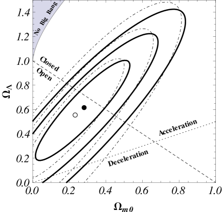
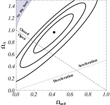
Figure 1: Solid lines shows 1$\sigma$, 2$\sigma$, and 3$\sigma$ constraint contours for the $\Lambda$CDM model from the $H(z)$ data. The left panel is for the $H_{0}=68\pm 2.8$ km s^-1 Mpc^-1 prior and the right panel is for the $H_{0}=73.8\pm 2.4$ km s^-1 Mpc^-1 one. Thin dot-dashed lines in the left panel are 1$\sigma$, 2$\sigma$, and 3$\sigma$ contours reproduced from, Yun & Ratra⁴⁴ where the prior is $H_{0}=68\pm 3.5$ km s^-1 Mpc^-1; the empty circle is the corresponding best-fit point. The dashed diagonal lines correspond to spatially-flat models, the dotted lines demarcate zero-acceleration models, and the shaded area in the upper left-hand corners are the region for which there is no big bang. The filled black circles correspond to best-fit points. For quantitative details see Table (1).

Figure 2: Solid lines shows 1$\sigma$, 2$\sigma$, and 3$\sigma$ constraint contours for the XCDM parametrization from the $H(z)$ data. The left panel is for the $H_{0}=68\pm 2.8$ km s^-1 Mpc^-1 prior and the right panel is for the $H_{0}=73.8\pm 2.4$ km s^-1 Mpc^-1 one. Thin dot-dashed lines in the left panel are 1$\sigma$, 2$\sigma$, and 3$\sigma$ contours reproduced from Yun & Ratra⁴⁴, where the prior is $H_{0}=68\pm 3.5$ km s^-1 Mpc^-1; the empty circle is the corresponding best-fit point. The dashed horizontal lines at $\omega_{\rm X}=-1$ correspond to spatially-flat $\Lambda$CDM models and the curved dotted lines demarcate zero-acceleration models. The filled black circles correspond to best-fit points. For quantitative details see Table (1).

Figure 3: Solid lines shows 1$\sigma$, 2$\sigma$, and 3$\sigma$ constraint contours for the $\phi$CDM model from the $H(z)$ data. The left panel is for the $H_{0}=68\pm 2.8$ km s^-1 Mpc^-1 prior and the right panel is for the $H_{0}=73.8\pm 2.4$ km s^-1 Mpc^-1 one. Thin dot-dashed lines in the left panel are 1$\sigma$, 2$\sigma$, and 3$\sigma$ contours reproduced from Yun & Ratra⁴⁴, where the prior is $H_{0}=68\pm 3.5$ km s^-1 Mpc^-1; the empty circle is the corresponding best-fit point. The horizontal axes at $\alpha=0$ correspond to spatially-flat $\Lambda$CDM models and the curved dotted lines demarcate zero-acceleration models. The filled black circles correspond to best-fit points. For quantitative details see Table (1).

$$t=\sqrt{\frac{1}{2}\alpha}\left[H_{0}-\frac{\beta}{\alpha}\right],\hskip 28.45274pt \Rightarrow \hskip 28.45274ptdH_{0}=\sqrt{\frac{2}{\alpha}}dt,$$

$$\mathrm{When,}\hskip 56.9055ptH_{0}=0\hskip 14.22636pt \Rightarrow \hskip 14.22636ptt=-\frac{\beta}{\sqrt{2\alpha}},$$ (11)

$$\mathrm{When,}\hskip 48.36958ptH_{0}\rightarrow\infty\hskip 14.22636pt \Rightarrow \hskip 14.22636ptt\rightarrow\infty.$$

Thus we can write the posterior likelihood function $\mathcal{L}_{H}(\textbf{p})$ as:

$$\mathcal{L}_{H}(\textbf{p}) = \frac{1}{\sqrt{\cancel{2}\pi\sigma^{2}_{H_{0}}}}\mathrm{exp}\left[-\frac{1}{2}\left(\gamma-\frac{\beta^{2}}{\alpha}\right)\right]\int\limits^{\infty}_{-\beta/\sqrt{2\alpha}}e^{-t^{2}}\left(\frac{\sqrt{\cancel{2}}}{\alpha}\right)dt,$$ (12)

$$= \frac{1}{\sqrt{\alpha\pi\sigma^{2}_{H_{0}}}}\mathrm{exp}\left[-\frac{1}{2}\left(\gamma-\frac{\beta^{2}}{\alpha}\right)\right]\left[\int\limits^{\beta/\sqrt{2\alpha}}_{0}e^{-t^{2}}dt+\int\limits^{\infty}_{0}e^{-t^{2}}dt\right].$$

Using the definition of error function, and the very commonly known result, that the second integral in square brackets of above equation is $\sqrt{\pi}/2$, we get:

$$\mathcal{L}_{H}(\textbf{p})=\frac{1}{2\sqrt{\alpha~{}\sigma_{H_{0}}^{2}}}\exp\left[-\frac{1}{2}\left({\gamma}-\frac{\beta^{2}}{\alpha}\right)\right]\left[1+\mathrm{erf}\left({\frac{\beta}{\sqrt{2\alpha}}}\right)\right].$$ (13)

We maximize the likelihood $\mathcal{L}_{H}(\textbf{p})$, or equivalently minimize $\chi_{H}^{2}(\textbf{p})=-2\mathrm{ln}\mathcal{L}_{H}(\textbf{p})$, with respect to the parameters p to find the best-fit parameter values $\mathbf{p_{0}}$. In the models we consider $\chi_{H}^{2}$ depends on two parameters. We define 1$\sigma$, 2$\sigma$, and 3$\sigma$ confidence intervals as two-dimensional parameter sets bounded by $\chi_{H}^{2}(\textbf{p})=\chi_{H}^{2}(\mathbf{p_{0}})+2.3,~{}\chi_{H}^{2}(\textbf{p})=\chi_{H}^{2}(\mathbf{p_{0}})+6.17$, and $\chi_{H}^{2}(\textbf{p})=\chi_{H}^{2}(\mathbf{p_{0}})+11.8$, respectively.

Even though the precision of measurements of the Hubble constant have greatly improved over the last decade, the concomitant improvement in the precision of other cosmological measurements means that in some cases the Hubble constant uncertainty still significantly affects cosmological parameter estimation. For a recent example see Calabrese et al.²⁶ The values of $\bar{H_{0}}\pm\sigma_{H_{0}}$ that we use in this paper are 68 $\pm$ 2.8 km s^-1 Mpc^-1 and 73.8 $\pm$ 2.4 km s^-1 Mpc^-1. The first is from a median statistics analysis Gott et al.⁸³ of 553 measurements of $H_{0}$ Chen et al.;⁴³ this estimate has been remarkably stable for over a decade now ⁸³, ⁴⁰. The second value is the most precise recent one, based on HST measurements Riess et al.¹⁴⁵. Other recent measurements are not inconsistent with at least one of the two values we use as a prior see, e.g., Freedman et al.,⁶⁷ Sorce et al.,¹⁶³ and Tammann et al.¹⁶⁹

Model and prior	$H(z)$		SNeIa		BAO
	$\chi^{2}_{\rm min}$	B.F.P	$\chi^{2}_{\rm min}$	B.F.P	$\chi^{2}_{\rm min}$	B.F.P
$\Lambda$CDM	$14.6$	$\Omega_{m0}=0.28$	545	$\Omega_{m0}=0.29$	5.5	$\Omega_{m0}=0.27$
$h=0.68\pm 0.028$		$\Omega_{\Lambda}=0.62$
$\Lambda$CDM	$14.6$	$\Omega_{m0}=0.42$		$\Omega_{\Lambda}$=0.69		$\Omega_{\Lambda}$=0.87
$h=0.738\pm 0.024$		$\Omega_{\Lambda}=0.97$
XCDM	$14.6$	$\Omega_{m0}=0.31$	545	$\Omega_{m0}=0.29$	$5.5$	$\Omega_{m0}=0.27$
$h=0.68\pm 0.028$		$\omega_{X}=-0.94$
XCDM	$14.6$	$\Omega_{m0}=0.30$		$\omega_{X}=-0.99$		$\omega_{X}=-1.21$
$h=0.738\pm 0.024$		$\omega_{X}=-1.3$
$\phi$CDM	$14.6$	$\Omega_{m0}=0.30$	545	$\Omega_{m0}=0.27$	5.9	$\Omega_{m0}=0.30$
$h=0.68\pm 0.028$		$\alpha=0.25$
$\phi$CDM	$15.6$	$\Omega_{m0}=0.27$		$\alpha=0.20$		$\alpha=0.00$
$h=0.738\pm 0.024$		$\alpha=0.00$

Table 1: The minimum value of $\chi^{2}$ and the corresponding best-fit points (B.F.P) that maximize the likelihood for the three individual data sets. The SNIa values are for the case including systematic errors. Ignoring SNIa systematic errors, for the $\Lambda$CDM model $\chi_{SN}^{2}(\mathbf{p_{0}})=562$, at $(\Omega_{m0},\Omega_{\Lambda})=(0.28,0.73)$; for the XCDM case $\chi_{SN}^{2}(\mathbf{p_{0}})=562$ at $(\Omega_{m0},\omega_{\rm X})=(0.28,-1.01)$; and for the $\phi$CDM model $\chi_{SN}^{2}(\mathbf{p_{0}})=562$, at $(\Omega_{m0},\alpha)=(0.27,0.05)$.

Figures (1)—(3) show the constraints from the $H(z)$ data for the three dark energy models we consider, and for the two different $H_{0}$ priors. Table (1) lists the best fit parameter values. Comparing these plots with Figs. 1—3 of Yun & Ratra,⁴⁴ whose 1$\sigma$, 2$\sigma$ and 3$\sigma$ constraint contours are reproduced here as dot-dashed lines in the left panels of Figs (1)—(3), we see that the contours derived from the new data are more constraining, by about a standard deviation, because of the 8 new, more precise, data points used here taken from Moresco et al.¹¹² On comparing the left and right panels in these three figures, we see that the constraint contours are quite sensitive to the value of $H_{0}$ used, as well as to the uncertainty associated with the Hubble constant measurement.

3 Constraints from the SNIa Data

While the $H(z)$ data provide tight constraints on a linear combination of cosmological parameters, the very elongated constraint contours of Figs. (1)—(3) imply that these data alone cannot significantly discriminate between cosmological models. To tighten the constraints we must add other data to the mix.

The second set of data that we use are the Type Ia supernova data from the Suzuki et al.¹⁶⁸ Union2.1 compilation of 580 SNIa distance modulus $\mu_{\rm obs}(z_{i})$ measurements at measured redshifts $z_{i}$ (covering the redshift range of 0.015 to 1.414) with associated one standard deviation uncertainties $\sigma_{i}$. The predicted distance modulus from Eq. (40) is:

$$\mu_{\rm th}(z_{i};H_{0},\textbf{p})=\underbrace{5~{}\mathrm{log}_{10}\left(3000~{}y(z)(1+z)\right)+25}_{=\mu_{0}}~{}-\ 5~{}\mathrm{log}_{10}(h),$$ (14)

where $H_{0}=100h$ km s^-1 Mpc^-1 and $y(z)$ is the dimensionless coordinate distance given in Eq. (13) as:

$$y(z)=\left\{\begin{array}[]{lc}\frac{a_{0}H_{0}}{\sqrt{k}}\mathrm{sin}\left(\frac{\sqrt{k}}{a_{0}H_{0}}\int\limits^{z}_{0}\frac{dz^{\prime}}{E(z^{\prime})}\right)&\ \ \ \ \mathrm{for}\ k>0\\ \int\limits^{z}_{0}\frac{dz^{\prime}}{E(z^{\prime})}&\ \ \ \ \mathrm{for}\ k=0\\ \frac{a_{0}H_{0}}{\sqrt{-k}}\mathrm{sinh}\left(\frac{\sqrt{-k}}{a_{0}H_{0}}\int\limits^{z}_{0}\frac{dz^{\prime}}{E(z^{\prime})}\right)&\ \ \ \ \mathrm{for}\ k<0\\ \end{array}.\right.$$ (15)

As the SNIa distance modulus measurements $\mu_{\rm obs}$ are correlated, $\chi^{2}$ is defined as:

$$\chi_{SN}^{2}(h,\textbf{p})=\Delta\boldsymbol{\mu}^{T}~{}{\mathcal{C}}^{-1}~{}\Delta\boldsymbol{\mu}.$$ (16)

Here $\Delta\boldsymbol{\mu}$ is a vector of differences $\Delta{\mu_{i}}=\mu_{\rm th}(z_{i};H_{0},\textbf{p})-\mu_{\rm obs}(z_{i})$, and $\mathcal{C}^{-1}$ is the inverse of the 580 by 580 Union 2.1 compilation covariance matrix. In index notation:

$$\chi^{2}_{SN}(h,\textbf{p})=\sum_{\alpha,\beta}\left[\mu_{0}-5\mathrm{log}_{10}h-\mu_{\rm obs}\right]_{\alpha}(\mathcal{C}^{-1})_{\alpha\beta}\left[\mu_{0}-5\mathrm{log}_{10}h-\mu_{\rm obs}\right]_{\beta}.$$ (17)

Let’s simplify this:

$$\chi^{2}_{SN}(h,\textbf{p}) = \sum\limits_{\alpha\beta}\left[\mu_{0}-\mu_{\mathrm{obs}}\right]_{\alpha}(\mathcal{C}^{-1})_{\alpha\beta}\left[\mu_{0}-\mu_{\mathrm{obs}}\right]_{\beta}-\big{(}5\mathrm{log}_{10}h\big{)}\left[\sum\limits_{\alpha\beta}\left[\mu_{0}-\mu_{\mathrm{obs}}\right]_{\alpha}(\mathcal{C}^{-1})_{\alpha\beta}\right]$$ (18)

$$-\big{(}5\mathrm{log}_{10}h\big{)}\left[(\mathcal{C}^{-1})_{\alpha\beta}\sum\limits_{\alpha\beta}\left[\mu_{0}-\mu_{\mathrm{obs}}\right]_{\beta}\right]+\big{(}5\mathrm{log}_{10}h\big{)}^{2}\sum\limits_{\alpha\beta}(\mathcal{C}^{-1})_{\alpha\beta},$$

since the the covariance matrix is symmetric hence the second and the third terms in above equation will just add, an we will get:

$$\chi^{2}_{SN}(h,\textbf{p}) = \sum\limits_{\alpha\beta}\left[\mu_{0}-\mu_{\mathrm{obs}}\right]_{\alpha}(\mathcal{C}^{-1})_{\alpha\beta}\left[\mu_{0}-\mu_{\mathrm{obs}}\right]_{\beta}-\big{(}10\mathrm{log}_{10}h\big{)}\left[(\mathcal{C}^{-1})_{\alpha\beta}\sum\limits_{\alpha\beta}\left[\mu_{0}-\mu_{\mathrm{obs}}\right]_{\beta}\right]$$ (19)

$$+\big{(}5\mathrm{log}_{10}h\big{)}^{2}\sum\limits_{\alpha\beta}(\mathcal{C}^{-1})_{\alpha\beta},$$

Defining:

$$\begin{array}[]{lr}A(\textbf{p})=\sum\limits_{\alpha,\beta}(\mu_{0}-\mu_{\rm obs})_{\alpha}\ (\mathcal{C}^{-1})_{\alpha\beta}\ (\mu_{0}-\mu_{\rm obs})_{\beta}\\ B(\textbf{p})=\sum\limits_{\alpha}(\mu_{0}-\mu_{\rm obs})_{\alpha}\sum\limits_{\beta}(\mathcal{C}^{-1})_{\alpha\beta}\\ C=\sum\limits_{\alpha,\beta}(\mathcal{C}^{-1})_{\alpha\beta}.\end{array}$$ (20)

then Eq. (19) takes the form:

$$\chi^{2}_{SN}(h,\textbf{p})=A(\textbf{p})-10B(\textbf{p})\mathrm{log}_{10}(h)+25C[\mathrm{log}_{10}(h)]^{2}$$ (21)

The corresponding likelihood function, when considering a flat $H_{0}$ prior, is:

$$\mathcal{L}_{SN}(\textbf{p}) = \int\limits_{0}^{\infty}{e^{-\chi^{2}_{SN}(h,\textbf{p})/2}dh},$$ (22)

$$= \mathrm{exp}\left[-\frac{1}{2}A(\textbf{p})\right]{{\int}}\limits^{\infty}_{0}\mathrm{exp}\left[-\frac{25C}{2}(\mathrm{log}_{10}h)^{2}+5B(\textbf{p})(\mathrm{log}_{10}h)\right]dh,$$

completing the square in the exponent results in:

$$\mathcal{L}_{SN}(\textbf{p}) = \mathrm{exp}\left[-\frac{1}{2}\left(A(\textbf{p})-\frac{B^{2}(\textbf{p})}{C}\right)\right]{{\int}}\limits^{\infty}_{0}\mathrm{exp}\left[-\frac{25C}{2}\left(\mathrm{log}_{10}h-\frac{B(\textbf{p})}{5C}\right)^{2}\right]dh.$$ (23)

Using the property of logarithm that $\mathrm{log_{10}}x=\frac{\mathrm{ln}x}{\mathrm{ln}10}$, we get:

$$\mathcal{L}_{SN}(\textbf{p}) = \mathrm{exp}\left[-\frac{1}{2}\left(A(\textbf{p})-\frac{B^{2}(\textbf{p})}{C}\right)\right]{{\int}}\limits^{\infty}_{0}\mathrm{exp}\left[-\frac{25C}{2}\left(\frac{\mathrm{ln}h}{\mathrm{ln}10}-\frac{B(\textbf{p})}{5C}\right)^{2}\right]dh,$$ (24)

simplifying we get:

$$\mathcal{L}_{SN}(\textbf{p}) = \mathrm{exp}\left[-\frac{1}{2}\left(A(\textbf{p})-\frac{B^{2}(\textbf{p})}{C}\right)\right]{{\int}}\limits^{\infty}_{0}\mathrm{exp}\left[-\frac{25C}{2\left(\mathrm{ln}10\right)^{2}}\left(\mathrm{ln}h-\frac{B(\textbf{p})(\mathrm{ln}10)}{5C}\right)^{2}\right]dh,$$ (25)

Defining:

$$\delta=\frac{25C}{2\mathrm{(ln10)^{2}}}~{},~{}~{}~{}\varepsilon=\frac{B(\textbf{p})\mathrm{ln10}}{5C},$$

$$\mathcal{L}_{SN}(\textbf{p}) = \mathrm{exp}\left[-\frac{1}{2}\left(A(\textbf{p})-\frac{B^{2}(\textbf{p})}{C}\right)\right]{{\int}}\limits^{\infty}_{0}\mathrm{exp}\Big{[}-\delta\big{(}\mathrm{ln}h-\varepsilon\big{)}^{2}\Big{]}dh.$$ (26)

Substituting:

$$\mathrm{ln}h-\varepsilon=y,\hskip 14.22636pt\Rightarrow\hskip 14.22636pth=e^{y+\varepsilon},$$ (27)

$$\Rightarrow\hskip 28.45274pt\frac{dh}{h}=dy,\hskip 14.22636pt\Rightarrow\hskip 14.22636ptdh=e^{y+\varepsilon}dy.$$ (28)

Using Eqs. (27) and (28), it is easy to see that:

$$\mathrm{When:} \hskip 14.22636pth\rightarrow 0,\hskip 28.45274pty\rightarrow-\infty,$$ (29)

$$\mathrm{When:} \hskip 14.22636pth\rightarrow\infty,\hskip 28.45274pty\rightarrow+\infty.$$ (30)

Thus the likelihood function takes the form:

$$\mathcal{L}_{SN}(\textbf{p}) = \mathrm{exp}\left[-\frac{1}{2}\left(A(\textbf{p})-\frac{B^{2}(\textbf{p})}{C}\right)\right]\int\limits^{\infty}_{-\infty}e^{-\delta y^{2}}e^{y+\varepsilon}dy,$$ (31)

$$= \mathrm{exp}\left[-\frac{1}{2}\left(A(\textbf{p})-\frac{B^{2}(\textbf{p})}{C}-2\varepsilon\right)\right]\int\limits^{\infty}_{-\infty}e^{-\delta\left(y^{2}-\frac{1}{\delta}y\right)}dy.$$

Completing the square in the exponent we will get:

$$\mathcal{L}_{SN}(\textbf{p}) = \mathrm{exp}\left[-\frac{1}{2}\left(A(\textbf{p})-\frac{B^{2}(\textbf{p})}{C}-2\varepsilon\right)\right]\int\limits^{\infty}_{-\infty}e^{-\delta\left(y^{2}-2\frac{1}{2\delta}y+\frac{1}{4\delta^{2}}-\frac{1}{4\delta^{2}}\right)}dy,$$ (32)

$$= \mathrm{exp}\left[-\frac{1}{2}\left(A(\textbf{p})-\frac{B^{2}(\textbf{p})}{C}-2\varepsilon-\frac{1}{2\delta}\right)\right]\int\limits^{\infty}_{-\infty}e^{-\delta\left(y-\frac{1}{2\delta}\right)^{2}}dy.$$

This is very standard integral called Gaussian integral.

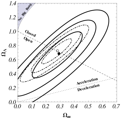
Figure 4: Thick solid (dot-dashed) lines are 1$\sigma$, 2$\sigma$, and 3$\sigma$ constraint contours from SNIa data with (without) systematic errors. Filled (open) circles demarcate likelihood maxima for the case of data with (without) systematic errors. The top left plot is for the $\Lambda$CDM model, the top right plot is for the XCDM parametrization, and the bottom one is for the $\phi$CDM model. For quantitative details see Table (1).

The above integral will come out to be:

$$\int\limits_{-\infty}^{\infty}e^{-\delta\left(y-\frac{1}{2\delta}\right)^{2}}dy=\sqrt{\frac{\pi}{\delta}}.$$ (34)

Hence, the likelihood function will become:

$$\mathcal{L}_{SN}(\textbf{p})=\sqrt{\frac{\pi}{\delta}}{\rm exp}\left[-\frac{1}{2}\left(A(\textbf{p})-\frac{B^{2}(\textbf{p})}{C}-2\varepsilon-\frac{1}{2\delta}\right)\right].$$ (35)

The $h$-independent:

$$\chi^{2}_{SN}(\textbf{p})=-2~{}\mathrm{ln}\mathcal{L}_{SN}(\textbf{p})=A(\textbf{p})-\frac{B^{2}(\textbf{p})}{C}-\frac{2\mathrm{ln}(10)}{5C}B(\textbf{p})-Q,$$ (36)

where $Q$ is a constant that does not depend on the model parameters p:

$$Q=\frac{2(\mathrm{ln}10)^{4}}{625~{}C^{2}}+2~{}\mathrm{ln}\left(\frac{2\pi(\mathrm{ln}10)^{2}}{25~{}C}\right),$$

and so can be ignored. We minimize $\chi_{SN}^{2}(\textbf{p})$ with respect to the model parameters p to find the best-fit parameter values $\mathbf{p_{0}}$ and constraint contours.

Figure (4) shows constraints from the SNIa data on the three dark energy models we consider here. For the $\Lambda$CDM model and the XCDM parametrization the constraints shown in Fig. (4) are in very good agreement with those in Figs. 5 and 6 of Suzuki et al.¹⁶⁸ The $\phi$CDM model SNIa data constraints shown in Fig. (4) have not previously been computed. Comparing the SNIa constraints of Fig. (4) to those which follow from the $H(z)$ data, Figs. (1)—(3), it is clear that SNIa data provide tighter constraints on the $\Lambda$CDM model. For the XCDM case both SNIa data and $H(z)$ data provide approximately similar constraints, while the SNIa constraints are somewhat more restrictive than the $H(z)$ ones for the $\phi$CDM model. However, in general, the SNIa constraints are not very significantly more restrictive than the $H(z)$ constraints, which is a remarkable result. It is also reassuring that both data favor approximately similar regions of parameters space, for all three models we consider. However, given that the degeneracy in parameter space is similar for the $H(z)$ and SNIa data, a joint analysis of just these two data sets is unlikely to greatly improve the constraints.

4 Constraints from the BAO Data

In an attempt to further tighten the cosmological parameter constraints, we now include BAO data in the analysis. To constrain cosmological parameters using BAO data we follow the procedure of Blake et al.¹⁹ To derive the BAO constraints we make use of the distance parameter $D_{V}(z)$, a combination of the angular diameter distance and the Hubble parameter, given by:

$$D_{V}(z)=\left[(1+z)^{2}d_{A}(z)^{2}\frac{c~{}z}{H(z)}\right]^{1/3}.$$ (37)

Here $d_{A}(z)$ is the angular diameter distance from Eq. (16):

$$d_{A}(z)=\frac{y(z)}{H_{0}(1+z)},$$ (38)

where $y(z)$ is the dimensionless coordinate distance given in Eq. (15).

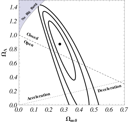
Figure 5: 1$\sigma$, 2$\sigma$, and 3$\sigma$ constraint contours from the BAO data. Filled circles denote likelihood maxima. The top left plot is for the $\Lambda$CDM model, the top right one is for the XCDM parametrization, and the bottom plot is for the $\phi$CDM model. For quantitative details see Table (1).

We use measurements of the acoustic parameter $A(z)$ from Blake et al,¹⁹ where the theoretically-predicted $A_{\rm th}(z)$ is given in Eq. (5) of Eisenstein et al.:⁵⁷

$$A_{\rm th}(z)=\frac{100~{}D_{V}(z)~{}\sqrt{\Omega_{m}h^{2}}}{z}.$$ (39)

Using Eqs. (37)—(39) we have:

$$A_{\rm th}(z)=\sqrt{\Omega_{m}}\left[\frac{y^{2}(z)}{z^{2}E(z)}\right]^{1/3},$$ (40)

which is $h$ independent and where $E(z)$ is defined in Chapter (1).

Using the WiggleZ $A_{\rm obs}(z)$ data from Table (3) of Blake et al,¹⁹ we compute:

$$\chi_{A_{z}}^{2}(\textbf{p})=\Delta{\textbf{A}}^{T}({\rm C}_{A_{z}})^{-1}\Delta{\textbf{A}}.$$ (41)

Here $\Delta{\textbf{A}}$ is a vector consisting of differences $\Delta{A_{i}}=A_{\rm th}(z_{i};\textbf{p})-A_{\rm obs}(z_{i})$ and $({\rm C}_{Az})^{-1}$ is the inverse of the 3 by 3 covariance matrix given in Table (3) of Blake et al.¹⁹

We also use the 6dFGS and SDSS data, three measurements from Beutler et al,¹⁵ Percival et al,¹²³, listed in Blake et al.¹⁹ In this case the distilled parameter:

$$d_{\rm th}(z)=\frac{r_{s}(z_{d})}{D_{V}(z)},$$ (42)

where $r_{s}(z_{d})$ is the sound horizon at the drag epoch, is given in Eq. (6) of Eisenstein et al.⁵⁶ The correlation coefficients for this case are also given in Table (3) of Blake et al.¹⁹ Using the covariance matrix we define:

$$\chi_{d_{z}}^{2}(h,\textbf{p})=\Delta{\textbf{d}}^{T}({\rm C}_{d_{z}})^{-1}\Delta{\textbf{d}}$$ (43)

where $\Delta{\textbf{d}}$ is a vector consisting of differences $\Delta{d_{i}}=d_{\rm th}(z_{i};h,\textbf{p})-d_{\rm obs}(z_{i})$ and ${\rm C}_{d_{z}}$ is the the covariance matrix Blake et al..¹⁹ We then marginalize over a flat prior for $H_{0}$ to get:

$$\chi_{d_{z}}^{2}(\textbf{p})=-2~{}\mathrm{ln}\left[\int^{\infty}_{0}{e^{-\chi_{d_{z}}^{2}(h,\textbf{p})/2}dh}\right].$$ (44)

Since $\chi_{A_{z}}^{2}(\textbf{p})$ and $\chi_{d_{z}}^{2}(\textbf{p})$ correspond to independent data, the combined BAO data:

$$\chi_{BAO}^{2}(\textbf{p})=\chi_{A_{z}}^{2}(\textbf{p})+\chi_{d_{z}}^{2}(\textbf{p}).$$ (45)

We can maximize the likelihood by minimizing $\chi_{BAO}^{2}(\textbf{p})$ with respect to the model parameters p to get best-fit parameter values $\mathbf{p_{0}}$ and constraint contours. Figure (5) show the constraints from the BAO data on the three dark energy models we consider here. The XCDM parametrization constraints shown in this figure are in good agreement with those shown in Fig. 13 of Blake et al.¹⁹ The constraints shown in the other two panels of Fig. (5) have not previously been computed. Comparing to the $H(z)$ and SNIa constraint contours of Figs. (1)—(4), we see that the BAO contours are also very elongated, although largely orthogonal to the $H(z)$ and SNIa ones. Consequently, a joint analysis of these data will result in significantly tighter constraints than those derived using any one of these data sets.

5 Joint Constraints

To constrain cosmological parameters from a joint analysis of the $H(z)$, SNIa, and BAO data we compute:

$$\chi^{2}(\textbf{p})=\chi_{H}^{2}(\textbf{p})+\chi_{SN}^{2}(\textbf{p})+\chi_{BAO}^{2}(\textbf{p})$$ (46)

for each of the three cosmological models considered here. We minimize $\chi^{2}(\textbf{p})$ with respect to model parameters p to get best-fit parameter values $\mathbf{p_{0}}$ and constraint contours.

Figure 6: Thick solid (dot-dashed) lines are 1$\sigma$, 2$\sigma$, and 3$\sigma$ constraint contours for the $\Lambda$CDM model from a joint analysis of the BAO and SNIa (with systematic errors) data, with (without) the $H(z)$ data. The full (empty) circle marks the best-fit point determined from the joint analysis with (without) the $H(z)$ data. The dotted sloping line corresponds to spatially-flat $\Lambda$CDM models. In the left panel we use the $H_{0}$ = 68 $\pm$ 2.8 km s^-1 Mpc^-1 prior while the right panel is for the $H_{0}$ = 73.8 $\pm$ 2.4 km s^-1 Mpc^-1 case. For quantitative details see Table (2).

Figure 7: Thick solid (dot-dashed) lines are 1$\sigma$, 2$\sigma$, and 3$\sigma$ constraint contours for the XCDM parametrization from a joint analysis of the BAO and SNIa (with systematic errors) data, with (without) the $H(z)$ data. The full (empty) circle marks the best-fit point determined from the joint analysis with (without) the $H(z)$ data. The dotted horizontal line at $\omega_{\rm X}=-1$ corresponds to spatially-flat $\Lambda$CDM models. In the left panel we use the $H_{0}$ = 68 $\pm$ 2.8 km s^-1 Mpc^-1 prior while the right panel is for the $H_{0}$ = 73.8 $\pm$ 2.4 km s^-1 Mpc^-1 case. For quantitative details see Table (2).

Figure 8: Thick solid (dot-dashed) lines are 1$\sigma$, 2$\sigma$, and 3$\sigma$ constraint contours for the $\phi$CDM model from a joint analysis of the BAO and SNIa (with systematic errors) data, with (without) the $H(z)$ data. The full (empty) circle marks the best-fit point determined from the joint analysis with (without) the $H(z)$ data (in the left panel the full and empty circles overlap). The $\alpha=0$ horizontal axes correspond to spatially-flat $\Lambda$CDM models. In the left panel we use the $H_{0}$ = 68 $\pm$ 2.8 km s^-1 Mpc^-1 prior while the right panel is for the $H_{0}$ = 73.8 $\pm$ 2.4 km s^-1 Mpc^-1 case. For quantitative details see Table (2).

Model and prior	$H(z)$+BAO		$H(z)$+SNIa+BAO		SNIa+BAO
	$\chi^{2}_{\rm min}$	B.F.P	$\chi^{2}_{\rm min}$	B.F.P	$\chi^{2}_{\rm min}$	B.F.P
$\Lambda$CDM	$20.7$	$\Omega_{m0}=0.31$	566	$\Omega_{m0}=0.30$	$551$	$\Omega_{m0}=0.30$
$h=0.68\pm 0.028$		$\Omega_{\Lambda}=0.68$		$\Omega_{\Lambda}=0.70$
$\Lambda$CDM	$21.0$	$\Omega_{m0}=0.29$	567	$\Omega_{m0}=0.30$		$\Omega_{\Lambda}=0.73$
$h=0.738\pm 0.024$		$\Omega_{\Lambda}=0.79$		$\Omega_{\Lambda}=0.76$
XCDM	$20.7$	$\Omega_{m0}=0.31$	566	$\Omega_{m0}=0.31$	$551$	$\Omega_{m0}=0.30$
$h=0.68\pm 0.028$		$\omega_{X}=-0.99$		$\omega_{X}=-1.02$
XCDM	$20.8$	$\Omega_{m0}=0.28$	567	$\Omega_{m0}=0.30$		$\omega_{X}=-1.03$
$h=0.738\pm 0.024$		$\omega_{X}=-1.19$		$\omega_{X}=-1.08$
$\phi$CDM	$20.7$	$\Omega_{m0}=0.31$	566	$\Omega_{m0}=0.30$	551	$\Omega_{m0}=0.30$
$h=0.68\pm 0.028$		$\alpha=0.05$		$\alpha=0.00$
$\phi$CDM	$22.0$	$\Omega_{m0}=0.29$	567	$\Omega_{m0}=0.29$		$\alpha=0.00$
$h=0.738\pm 0.024$		$\alpha=0.00$		$\alpha=0.00$

Table 2: The minimum value of $\chi^{2}$ and the corresponding best fit points (B.F.P) which maximize the likelihood, for different combinations of data. The SNIa data values are for the case including systematic errors.

Figure 9: Thick solid (dot-dashed) lines are 1$\sigma$, 2$\sigma$, and 3$\sigma$ constraint contours for the $\Lambda$CDM model from a joint analysis of the BAO and $H(z)$ data, with (without) the SNIa data. The full (empty) circle marks the best-fit point determined from the joint analysis with (without) the SNIa data. The dotted sloping line corresponds to spatially-flat $\Lambda$CDM models. In the left panel we use the $H_{0}$ = 68 $\pm$ 2.8 km s^-1 Mpc^-1 prior while the right panel is for the $H_{0}$ = 73.8 $\pm$ 2.4 km s^-1 Mpc^-1 case. For quantitative details see Table (2).

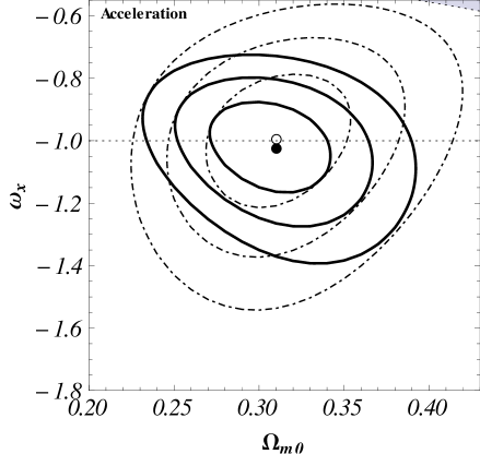
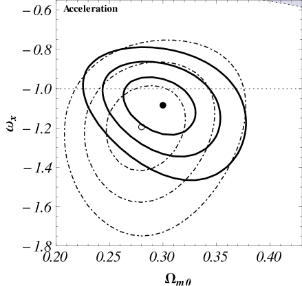
Figure 10: Thick solid (dot-dashed) lines are 1$\sigma$, 2$\sigma$, and 3$\sigma$ constraint contours for the XCDM parametrization from a joint analysis of the BAO and $H(z)$ data, with (without) the SNIa data. The full (empty) circle marks the best-fit point determined from the joint analysis with (without) the SNIa data. The dotted horizontal line at $\omega_{\rm X}=-1$ corresponds to spatially-flat $\Lambda$CDM models. In the left panel we use the $H_{0}$ = 68 $\pm$ 2.8 km s^-1 Mpc^-1 prior while the right panel is for the $H_{0}$ = 73.8 $\pm$ 2.4 km s^-1 Mpc^-1 case. The shaded area in the upper right corners are the region of decelerating expansion. For quantitative details see Table (2).

Figure 11: Thick solid (dot-dashed) lines are 1, 2, and 3 $\sigma$ constraint contours for the $\phi$CDM model from a joint analysis of the $H(z)$ and BAO data, with (without) the SNIa data. The full (empty) circle marks the best-fit point determined from the joint analysis with (without) the SNIa data. The $\alpha=0$ horizontal axes correspond to spatially-flat $\Lambda$CDM models. In the left panel we use the $H_{0}$ = 68 $\pm$ 2.8 km s^-1 Mpc^-1 prior while the right panel is for the $H_{0}$ = 73.8 $\pm$ 2.4 km s^-1 Mpc^-1 case. For quantitative details see Table (2).

Figures (6)—(8) show constraints on the cosmological parameters for the $\Lambda$CDM and $\phi$CDM models and the XCDM parametrization, from a joint analysis of the BAO and SNIa data, as well as from a joint analysis of the BAO, SNIa and $H(z)$ data. Table 3 lists information about best-fit parameter values. Including the $H(z)$ data in the analysis tightens the constraints by more than one standard deviation, in parts of the parameter spaces.

Model and prior	SNIa+BAO	$H(z)$+BAO	$H(z)$+SNIa+BAO
$\Lambda$CDM	0.25 $<$ $\Omega_{m0}$ $<$ 0.36	0.25 $<$ $\Omega_{m0}$ $<$ 0.36	0.26 $<$ $\Omega_{m0}$ $<$ 0.36
$h=0.68\pm 0.028$	0.53 $<$ $\Omega_{\Lambda}$ $<$ 0.89	0.45 $<$ $\Omega_{\Lambda}$ $<$ 0.85	0.55 $<$ $\Omega_{\Lambda}$ $<$ 0.83
$\Lambda$CDM	0.25 $<$ $\Omega_{m0}$ $<$ 0.36	0.23 $<$ $\Omega_{m0}$ $<$ 0.38	0.25 $<$ $\Omega_{m0}$ $<$ 0.35
$h=0.738\pm 0.024$	0.53 $<$ $\Omega_{\Lambda}$ $<$ 0.89	0.60 $<$ $\Omega_{\Lambda}$ $<$ 0.92	0.62 $<$ $\Omega_{\Lambda}$ $<$ 0.88
XCDM	0.30 $<$ $\Omega_{m0}$ $<$ 0.38	0.26 $<$ $\Omega_{m0}$ $<$ 0.37	0.29 $<$ $\Omega_{m0}$ $<$ 0.37
$h=0.68\pm 0.028$	$-1.18<\omega_{\rm X}<-0.78$	$-1.32<\omega_{\rm X}<-0.73$	$-1.14<\omega_{\rm X}<-0.78$
XCDM	0.30 $<$ $\Omega_{m0}$ $<$ 0.38	0.24 $<$ $\Omega_{m0}$ $<$ 0.35	0.27 $<$ $\Omega_{m0}$ $<$ 0.35
$h=0.738\pm 0.024$	$-1.18<\omega_{\rm X}<-0.78$	$-1.42<\omega_{\rm X}<-0.88$	$-1.22<\omega_{\rm X}<-0.86$
$\phi$CDM	0.25 $<$ $\Omega_{m0}$ $<$ 0.35	0.25 $<$ $\Omega_{m0}$ $<$ 0.36	0.26 $<$ $\Omega_{m0}$ $<$ 0.35
$h=0.68\pm 0.028$	0 $<$ $\alpha$ $<$ 0.54	0 $<$ $\alpha$ $<$ 1.01	0 $<$ $\alpha$ $<$ 0.54
$\phi$CDM	0.25 $<$ $\Omega_{m0}$ $<$ 0.35	0.23 $<$ $\Omega_{m0}$ $<$ 0.35	0.25 $<$ $\Omega_{m0}$ $<$ 0.33
$h=0.738\pm 0.024$	0 $<$ $\alpha$ $<$ 0.54	0 $<$ $\alpha$ $<$ 0.57	0 $<$ $\alpha$ $<$ 0.35

Table 3: Two standard deviation bounds on cosmological parameters using SNIa+BAO, $H(z)$+BAO and SNIa+BAO+$H(z)$ data, for three different models with two different $H_{0}$ priors.

Adding the $H(z)$ data for the $\bar{H_{0}}\pm\sigma_{H_{0}}=68\pm 2.8$ km s^-1 Mpc^-1 prior case improved the constraints most significantly in the $\Lambda$CDM case (by more than 1$\sigma$ on $\Omega_{\Lambda}$ in parts of parameter space), Fig. (6), and least significantly for the $\phi$CDM model, Fig. (8). For the case of the $\bar{H_{0}}\pm\sigma_{H_{0}}=73.8\pm 2.4$ km s^-1 Mpc^-1 prior, adding $H(z)$ again tightens up the constraints the most for the $\Lambda$CDM model (by more than 1$\sigma$ on $\Omega_{\Lambda}$), Fig. (6), and least so for the XCDM parametrization, Fig. (7).

Figures (9)—(11) show the constraints on the cosmological parameters of the three models, from a joint analysis of the BAO and $H(z)$ data, as well as from a joint analysis of the three data sets. Table (2) lists the best-fit parameter values. Comparing these figures to Figs. (6)—(8) allows for a comparison between the discriminating power of the SNIa and $H(z)$ data.

Figure (9) shows that adding SNIa data to the $H(z)$ and BAO data combination for the $\bar{H_{0}}\pm\sigma_{H_{0}}=68\pm 2.8$ km s^-1 Mpc^-1 prior case tightens up the constraints by more than 1$\sigma$ on $\Omega_{\Lambda}$ from below, while addition of SNIa data for the $\bar{H_{0}}\pm\sigma_{H_{0}}=73.8\pm 2.4$ km s^-1 Mpc^-1 prior case tightens up the constraints by more than 1$\sigma$ on $\Omega_{\Lambda}$ from above. Addition of SNIa data to the $H(z)$ and BAO combination doesn’t much improve the constraints on $\Omega_{m0}$ for either prior.

Figures (9)—(11) show that adding SNIa data to the $H(z)$ and BAO combination results in the most prominent effect for the XCDM case, Fig. (10). Here for the $\bar{H_{0}}\pm\sigma_{H_{0}}=68\pm 2.8$ km s^-1 Mpc^-1 prior it tightens up the constraints by more than 1$\sigma$ on $\omega_{X}$ from above and below while for the $\bar{H_{0}}\pm\sigma_{H_{0}}=73.8\pm 2.4$ km s^-1 Mpc^-1 prior it tightens up the constraints by more than 2 $\sigma$ on $\omega_{X}$ from below. Addition of SNIa data to the $H(z)$ and BAO combination doesn’t much improve the constraints on $\Omega_{m0}$ for either prior in this case.

In the $\phi$CDM case, Fig. (11), adding SNIa data to $H(z)$ and BAO combination affects the constraint on $\alpha$ the most for the $\bar{H_{0}}\pm\sigma_{H_{0}}=68\pm 2.8$ km s^-1 Mpc^-1 prior case. The effect on $\Omega_{m0}$ is little stronger than what happens in the $\Lambda$CDM and XCDM cases but still less than 1$\sigma$.

Table (3) lists the two standard deviation bounds on the individual cosmological parameters, determined from their one-dimensional posterior probability distributions functions (which are derived by marginalizing the two-dimensional likelihood over the other cosmological parameter) for different combinations of data set.

The constraints on the cosmological parameters that we derive from only the BAO and SNIa data are restrictive, but less so than those shown in Fig. 4 of Yun & Ratra.⁴⁴ This is because the new Suzuki et al.¹⁶⁸ SNIa compilation data we use here is based on a more careful accounting of the systematic errors, which have increased. Consequently, including the $H(z)$ data, in addition to the BAO and SNIa data, in the analysis, more significantly tightens the constraints: compare Figs. (6)—(8) here to Figs. 4—6 of Yun & Ratra.⁴⁴ We emphasize, however, that this effect is prominent only in some parts of the parameter spaces.

6 Conclusion

In summary, the results of a joint analysis of the $H(z)$, BAO, and SNIa data are very consistent with the predictions of a spatially-flat cosmological model with energy budget dominated by a time-independent cosmological constant, the standard $\Lambda$CDM model. However, the data are not yet good enough to strongly rule out slowly-evolving dark energy density. More, and better quality, data are needed to discriminate between constant and slowly-evolving dark energy density.

It is probably quite significant that current $H(z)$ data constraints are almost as restrictive as those from SNIa data. The acquisition of $H(z)$ data has been an interesting backwater of cosmology for the last few years. We hope that our results will help promote more interest in this exciting area. Since the $H(z)$ technique has not been as much studied as, say, the SNIa apparent magnitude technique, a little more effort in the $H(z)$ area is likely to lead to very useful results.

7 Addition of ${z=2.3}$ Data Point

At the same time when we were doing the above analysis Nicolâs Busca and his team²⁴ did the measurements of Hubble parameter $z$ at the high redshift $(z=2.3)$ using the Lyman $\alpha$ forest baryon acoustic oscillations measurements. Here we want to briefly describe the Lyman $\alpha$ forest which is becoming a very useful source of information in physical cosmology.

The Lyman series is the series of energies required to excite an electron in the (neutral) hydrogen atom from its lowest energy state (n=1) to any higher energy state. The case of particular interest for cosmology is where a hydrogen atom with its electron in the lowest energy configuration n=1, gets hit by a photon (electromagnetic wave coming probably from a quasar behind the gas cloud) and is excited to the next lowest energy level n=2. The energy levels are given by $E_{\mathrm{n}}=-13.6\mathrm{eV}/{\mathrm{n}}^{2}$ using Bohr’s theory of atomic model, see Fig. (12), and the energy difference between the lowest $(n=1)$ and second lowest $(n=2$) levels corresponds to a photon with wavelength 1216 $\AA$ $\approx$ 122 nm. The reverse process i.e., emission of the photon and hence energy, after the electron jumps from $n=2$ to $n=1$ can and does occur as well.

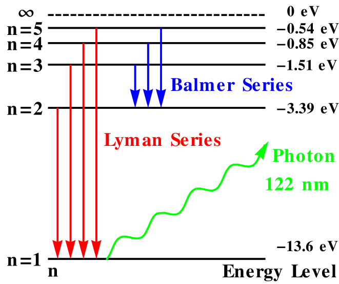
Figure 12: Energy levels of neutral hydrogen atom. The transition to $n=1$ shell from any other shell is called the Lyman series while the transition from any higher then $n=2$ shell to $n=2$ shell is called the Balmer series that lies in visible (blue) range. When an electron jumps from any excited shell of the hydrogen atom to the ground level $(n=1)$ it emits a photon. If the transition is from $n=2$ to $n=1$ then the wavelength of the photon is calculated to be 122 nm from Bohr’s theory.

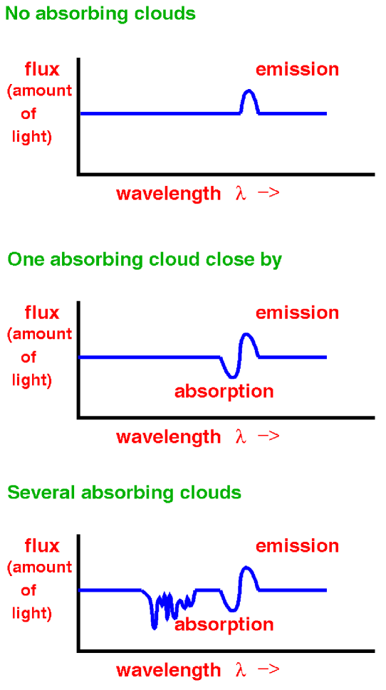
Figure 13: Top picture shows a cartoon of how a quasar spectrum (the flux of light as a function of wavelength) might look if there were no intervening neutral hydrogen between the quasars and us. The middle picture shows the flux for one nearby region, while the bottom picture shows the case for several intervening regions.

The absorption or emission of photons with the correct wavelength can tell us something about the presence of hydrogen and free electrons in space. That is, if you shine a light with wavelength 122 nm at a bunch of neutral hydrogen atoms, in their ground state, the atoms will absorb the light, using it to boost the electron to a higher energy state. If there are a lot of neutral hydrogen atoms in their ground state n=1, they will absorb more and more of the light (photons of this particular wavelength). So if you look at the light you receive and view the intensity as a function of wavelength, you will see a dip in the intensity at 122 nm. This dip in the intensity is dependent on the amount of neutral hydrogen present in its ground state. The amount of light absorbed, the optical depth is proportional to the probability that the hydrogen will absorb the photon (cross-section) times the number of hydrogen atoms along its path.

Since the Universe has many high energy photons and hydrogen atoms, both the absorption and emission of photons occurs frequently. In Lyman $\alpha$ systems, the hydrogen is found in regions in space, and the source for the photons are quasars (also called QSOs), very high energy light sources, shining at us from behind these regions.

Because the Universe is expanding, one can learn more than just the number of neutral hydrogen atoms between us and the quasar. As these photons travel to us, the Universe expands, stretching out all the light waves. This increases the wavelength $\lambda$ and lowers the energies of the photons.

Neutral hydrogen atoms in their lowest state will interact with whatever light has been red-shifted to a wavelength of 122 nm when it reaches them. The rest of the light will keep traveling to us.

The quasar shines with a certain spectrum or distribution of energies, with a certain amount of power in each wavelength. In Fig. (13) the top picture shows a cartoon of how a quasar spectrum (the flux of light as a function of wavelength) would look if there were no intervening neutral hydrogen between the quasar and us. In reality, gas around the quasar both emits and absorbs photons. With the presence of neutral hydrogen, including that near the quasar, the emitted flux is depleted for certain wavelengths, indicating the absorption by this intervening neutral hydrogen. As the 122 nm wavelength is preferably absorbed, we know that at the location the photon is absorbed, its wavelength is probably 122 nm. Its wavelength was stretched by the expansion of the Universe from what it was initially at the quasar, and, if it had continued to travel to us, it would have been stretched some more from the 122 nm wavelength it had at the absorber. Thus we see the dip in flux at the wavelength corresponding to that which the 122 nm (when it was absorbed) photon would have had if it had reached us. As we can calculate how the Universe is expanding, we can tell where the photons were absorbed in relation to us. Thus one can use the absorption map to plot the positions of region of intervening hydrogen between us and the quasar. The middle picture in Fig. (13) shows the flux for one nearby region while the bottom picture shows the case for several intervening regions. It is common to see absorption systems spread out into a ‘forest’ of lines because each line is red-shifted by a different amount in proportion to the absorbing cloud’s distance from us.

Hence, Busca et al.²⁴ reported the value of Hubble parameter $H$ at high redshift $z=2.3$ using the combined constraints from WMAP, CMB anisotropy, and baryon acoustic oscillations peak in the Ly$\alpha$ forest, when the Universe was matter dominated, as $H(z=2.3)=224\pm 8$ kms^-1 Mpc^-1. The analysis was based on 48,600 quasars which are at $1.96\leq z\leq 3.38$.

We decided to use this data point which has only 4% error to get improved constraints on the dark energy model parameters. With the addition this high redshift $H(z)$ data point our whole $H(z)$ data look like Table (2).

8 Improved Constraints

To constrain cosmological parameters p of the models of interest we follow the procedure of discussed above in this chapter Farooq et al.⁶⁰

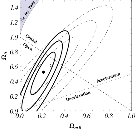
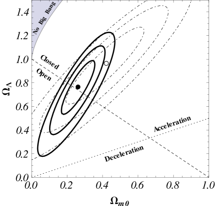
Figure 14: Thick solid (thin dot-dashed) lines correspond to 1$\sigma$, 2$\sigma$, and 3$\sigma$ constraint contours from the new (old, Farooq et al.⁶⁰) $H(z)$ data for the $\Lambda$CDM model. The filled (empty) circle is the best fit point from the new (old) $H(z)$ data. The left panel is for the $H_{0}=68\pm 2.8$ km s^-1 Mpc^-1 prior and the right panel is for the $H_{0}=73.8\pm 2.4$ km s^-1 Mpc^-1 one. The dashed diagonal lines correspond to spatially-flat models, the dotted lines demarcate zero-acceleration models, and the shaded area in the upper left-hand corners are the region for which there is no big bang. The filled circles correspond to best-fit pair $(\Omega_{m0},\Omega_{\Lambda})=(0.21,0.53)$ with $\chi^{2}_{\rm min}=15.1$ (left panel) and best-fit pair $(\Omega_{m0},\Omega_{\Lambda})=(0.26,0.77)$ with $\chi^{2}_{\rm min}=16.1$ (right panel). The empty circles correspond to best-fit pair $(\Omega_{m0},\Omega_{\Lambda})=(0.28,0.62)$ with $\chi^{2}_{\rm min}=14.6$ (left panel) and best-fit pair $(\Omega_{m0},\Omega_{\Lambda})=(0.42,0.97)$ with $\chi^{2}_{\rm min}=14.6$ (right panel).

Figure 15: Thick solid (thin dot-dashed) lines correspond to 1$\sigma$, 2$\sigma$, and 3$\sigma$ constraint contours from the new (old, Farooq et al.⁶⁰) $H(z)$ data for the XCDM model. The filled (empty) circle is the best fit point from the new (old) $H(z)$ data. The left panel is for the $H_{0}=68\pm 2.8$ km s^-1 Mpc^-1 prior and the right panel is for the $H_{0}=73.8\pm 2.4$ km s^-1 Mpc^-1 one. The dashed horizontal lines at $\omega_{\rm X}=-1$ correspond to spatially-flat $\Lambda$CDM models and the curved dotted lines demarcate zero-acceleration models. The filled circles correspond to best-fit pair $(\Omega_{m0},\omega_{\rm X})=(0.27,-0.82)$ with $\chi^{2}_{\rm min}=15.2$ (left panel) and best-fit pair $(\Omega_{m0},\omega_{\rm X})=(0.36,-1.1)$ with $\chi^{2}_{\rm min}=15.9$ (right panel). The empty circles correspond to best-fit pair $(\Omega_{m0},\omega_{\rm X})=(0.31,-0.94)$ with $\chi^{2}_{\rm min}=14.6$ (left panel) and best-fit pair $(\Omega_{m0},\omega_{\rm X})=(0.30,-1.30)$ with $\chi^{2}_{\rm min}=14.6$ (right panel).

Figure 16: Thick solid (thin dot-dashed) lines correspond to 1$\sigma$, 2$\sigma$, and 3$\sigma$ constraint contours from the new (old, Farooq et al.⁶⁰) $H(z)$ data for the $\phi$CDM model. The filled (empty) circle is the best fit point from the new (old) $H(z)$ data. The left panel is for the $H_{0}=68\pm 2.8$ km s^-1 Mpc^-1 prior and the right panel is for the $H_{0}=73.8\pm 2.4$ km s^-1 Mpc^-1 one. The horizontal axes at $\alpha=0$ correspond to spatially-flat $\Lambda$CDM models and the curved dotted lines demarcate zero-acceleration models. The filled circles correspond to best-fit pair $(\Omega_{m0},\alpha)=(0.36,0.70)$ with $\chi^{2}_{\rm min}=15.2$ (left panel) and best-fit pair $(\Omega_{m0},\alpha)=(0.25,0)$ with $\chi^{2}_{\rm min}=16.1$ (right panel). The empty circles correspond to best-fit pair $(\Omega_{m0},\alpha)=(0.30,0.25)$ with $\chi^{2}_{\rm min}=14.6$ (left panel) and best-fit pair $(\Omega_{m0},\alpha)=(0.27,0)$ with $\chi^{2}_{\rm min}=15.6$ (right panel).

We again marginalize over the nuisance parameter $H_{0}$ using two different Gaussian priors with $\bar{H_{0}}\pm\sigma_{H_{0}}$= 68 $\pm$ 2.8 km s^-1 Mpc^-1 and with $\bar{H_{0}}\pm\sigma_{H_{0}}$= 73.8 $\pm$ 2.4 km s^-1 Mpc^-1. As discussed there, the Hubble constant measurement uncertainty can significantly affect cosmological parameter estimation for a recent example see, e.g., Calabrese et al.²⁶ The lower of the two values we use is from a median statistics analysis Gott et al.⁸³ of 553 measurements of $H_{0}$ Chen et al.⁴³; this estimate has been stable for over a decade now ⁸³, ⁴⁰. The other value is a recent, HST based one Riess et al.¹⁴⁵ Other recent estimates are compatible with at least one of the two values we use. See for example, Freedman et al.,⁶⁷ Sorce et al.,¹⁶³ and Tammann et al.¹⁶⁹

We maximize the likelihood $\mathcal{L}_{H}(\textbf{p})$ with respect to the parameters p to find the best-fit parameter values $\mathbf{p_{0}}$. In the models we consider $\chi_{H}^{2}=-2{\rm ln}\mathcal{L}_{H}(\textbf{p})$ depends on two parameters. We define 1$\sigma$, 2$\sigma$, and 3$\sigma$ confidence intervals as two-dimensional parameter sets bounded by $\chi_{H}^{2}(\textbf{p})=\chi_{H}^{2}(\mathbf{p_{0}})+2.3,~{}\chi_{H}^{2}(\textbf{p})=\chi_{H}^{2}(\mathbf{p_{0}})+6.17$, and $\chi_{H}^{2}(\textbf{p})=\chi_{H}^{2}(\mathbf{p_{0}})+11.8$, respectively.

Figures (14)—(16) show the constraints from the $H(z)$ data derived here, as well as those derived by Farooq et al., ⁶⁰ for the three dark energy models, and for the two different $H_{0}$ priors. Clearly, the $H(z=2.3)$ measurement of Busca et al. ²⁴ significantly tightens the constrains. Given that the nonrelativistic matter density is larger relative to the dark energy density at $z=2.3$, it is perhaps not unexpected that the Busca et al.²⁴ measurement tightens the constraints on $\Omega_{m0}$ much more significantly than it does for the constraints on the other parameter which more strongly affects the evolution of the dark energy density, see Figs. (15) and (16).

Figure 17: Thick solid (thin dot-dashed) lines are 1$\sigma$, 2$\sigma$, and 3$\sigma$ constraint contours for the $\Lambda$CDM model from a joint analysis of the BAO and SNIa (with systematic errors) data, with (without) the $H(z)$ data. The full (empty) circle marks the best-fit point determined from the joint analysis with (without) the $H(z)$ data. The dotted sloping line corresponds to spatially-flat $\Lambda$CDM models. In the left panel we use the $H_{0}$ = 68 $\pm$ 2.8 km s^-1 Mpc^-1 prior. Here the empty circle [no $H(z)$ data] corresponds to best-fit pair $(\Omega_{m0},\Omega_{\Lambda})=(0.30,0.73)$ with $\chi^{2}_{\rm min}=551$ while the full circle [with $H(z)$ data] indicates best-fit pair $(\Omega_{m0},\Omega_{\Lambda})=(0.29,0.72)$ with $\chi^{2}_{\rm min}=567$. In the right panel we use the $H_{0}$ = 73.8 $\pm$ 2.4 km s^-1 Mpc^-1 prior. Here the empty circle [no $H(z)$ data] corresponds to best-fit pair $(\Omega_{m0},\Omega_{\Lambda})=(0.30,0.73)$ with $\chi^{2}_{\rm min}=551$ while the full circle [with $H(z)$ data] demarcates best-fit pair $(\Omega_{m0},\Omega_{\Lambda})=(0.28,0.78)$ with $\chi^{2}_{\rm min}=568$.

Figure 18: Thick solid (thin dot-dashed) lines are 1$\sigma$, 2$\sigma$, and 3$\sigma$ constraint contours for the XCDM parametrization from a joint analysis of the BAO and SNIa (with systematic errors) data, with (without) the $H(z)$ data. The full (empty) circle marks the best-fit point determined from the joint analysis with (without) the $H(z)$ data. The dotted horizontal line at $\omega_{\rm X}=-1$ corresponds to spatially-flat $\Lambda$CDM models. In the left panel we use the $H_{0}$ = 68 $\pm$ 2.8 km s^-1 Mpc^-1 prior. Here the empty circle [no $H(z)$ data] corresponds to best-fit pair $(\Omega_{m0},\omega_{\rm X})=(0.30,-1.03)$ with $\chi^{2}_{\rm min}=551$, while the full circle [with $H(z)$ data] demarcates best-fit pair $(\Omega_{m0},\omega_{\rm X})=(0.29,-0.99)$ with $\chi^{2}_{\rm min}=568$. In the right panel we use the $H_{0}$ = 73.8 $\pm$ 2.4 km s^-1 Mpc^-1 prior. Here the empty circle [no $H(z)$ data] corresponds to best-fit pair $(\Omega_{m0},\omega_{\rm X})=(0.30,-1.03)$ with $\chi^{2}_{\rm min}=551$ while the full circle [with $H(z)$ data] indicates best-fit pair $(\Omega_{m0},\omega_{\rm X})=(0.28,-1.05)$ with $\chi^{2}_{\rm min}=569$.

Figure 19: Thick solid (thin dot-dashed) lines are 1$\sigma$, 2$\sigma$, and 3$\sigma$ constraint contours for the $\phi$CDM model from a joint analysis of the BAO and SNIa (with systematic errors) data, with (without) the $H(z)$ data. The full (empty) circle marks the best-fit point determined from the joint analysis with (without) the $H(z)$ data. The $\alpha=0$ horizontal axes correspond to spatially-flat $\Lambda$CDM models. In the left panel we use the $H_{0}$ = 68 $\pm$ 2.8 km s^-1 Mpc^-1 prior. Here the empty circle corresponds to best-fit pair $(\Omega_{m0},\alpha)=(0.30,0)$ with $\chi^{2}_{\rm min}=551$ while the full circle indicates best-fit pair $(\Omega_{m0},\alpha)=(0.29,0)$ with $\chi^{2}_{\rm min}=567$. In the right panel we use the $H_{0}$ = 73.8 $\pm$ 2.4 km s^-1 Mpc^-1 prior. Here the empty circle corresponds to best-fit pair $(\Omega_{m0},\alpha)=(0.30,0)$ with $\chi^{2}_{\rm min}=551$ while the full circle demarcates best-fit pair $(\Omega_{m0},\alpha)=(0.27,0)$ with $\chi^{2}_{\rm min}=569$.

Comparing the $H(z)$ constraints derived here, and shown in Figs. (14)—(16) here, to the SNIa constraints shown in Fig. (4), we see that the new $H(z)$ data constraints are significantly more restrictive than those that follow on using the SNIa data. This is a remarkable result. Qualitatively, because of the dependence on the $H_{0}$ prior and on the model used in the analysis, Figs. (14)—(16) show that the $H(z)$ data alone require accelerated cosmological expansion at approximately the two standard deviation confidence level.

While the $H(z)$ data provide tight constraints on a linear combination of cosmological parameters, the banana-like constraint contours of Figs. (14)—(16) imply that these data alone cannot significantly discriminate between cosmological models. To tighten the constraints we must add other data to the mix. Following Farooq et al. ⁶⁰, we derive constraints on cosmological parameters of the three models from a joint analysis of the $H(z)$ data with the 6 BAO peak length scale measurements of Percival et al.¹²³, Beutler et al. ¹⁵, and Blake et al.¹⁹, and the Union2.1 compilation of 580 SNIa apparent magnitude measurements (covering a redshift range $0.015<z<1.4$) from Suzuki et al.¹⁶⁸.

Figure 20: Measurements and predictions for $H(z)/(1+z)$ as a function of $z$. Dashed (dotted) lines show the predictions for the best-fit $\Lambda$CDM model from the combined BAO, SNIa, and $H(z)$ data analyses, with cosmological parameter values $(\Omega_{m0},\Omega_{\Lambda},h)=(0.29,0.72,0.68)[(0.28,0.78,0.738)]$.

Figures (17)—(19) show the constraints on cosmological parameters for the $\Lambda$CDM and $\phi$CDM models and the XCDM parametrization, from a joint analysis of the BAO and SNIa data, as well as from a joint analysis of the BAO, SNIa, and $H(z)$ data. Including the $H(z)$ data in the analysis tightens the constraints, somewhat significantly (sometimes by more than two standard deviations), in parts of the parameter spaces. Figure (20) shows the $H(z)$ data and the two best-fit $\Lambda$CDM models. The $H(z)$ data do support the idea of a deceleration to acceleration transition somewhere in the range $0.5<z<1$.

Model and prior	BAO+SNIa	BAO+SNIa+$H(z)$
$\Lambda$CDM, $h=0.68\pm 0.028$	0.25 $<$ $\Omega_{m0}$ $<$ 0.36	0.26 $<$ $\Omega_{m0}$ $<$ 0.33
	0.53 $<$ $\Omega_{\Lambda}$ $<$ 0.89	0.60 $<$ $\Omega_{\Lambda}$ $<$ 0.84
$\Lambda$CDM, $h=0.738\pm 0.024$	0.25 $<$ $\Omega_{m0}$ $<$ 0.36	0.25 $<$ $\Omega_{m0}$ $<$ 0.32
	0.53 $<$ $\Omega_{\Lambda}$ $<$ 0.89	0.66 $<$ $\Omega_{\Lambda}$ $<$ 0.89
XCDM, $h=0.68\pm 0.028$	0.30 $<$ $\Omega_{m0}$ $<$ 0.38	0.27 $<$ $\Omega_{m0}$ $<$ 0.32
	$-1.18<\omega_{\rm X}<-0.78$	$-1.03<\omega_{\rm X}<-0.77$
XCDM, $h=0.738\pm 0.024$	0.30 $<$ $\Omega_{m0}$ $<$ 0.38	0.25 $<$ $\Omega_{m0}$ $<$ 0.30
	$-1.18<\omega_{\rm X}<-0.78$	$-1.15<\omega_{\rm X}<-0.90$
$\phi$CDM, $h=0.68\pm 0.028$	0.25 $<$ $\Omega_{m0}$ $<$ 0.35	0.25 $<$ $\Omega_{m0}$ $<$ 0.32
	0 $<$ $\alpha$ $<$ 0.54	0 $<$ $\alpha$ $<$ 0.56
$\phi$CDM, $h=0.738\pm 0.024$	0.25 $<$ $\Omega_{m0}$ $<$ 0.35	0.25 $<$ $\Omega_{m0}$ $<$ 0.30
	0 $<$ $\alpha$ $<$ 0.54	0 $<$ $\alpha$ $<$ 0.21

Table 4: Two standard deviation bounds on cosmological parameters using BAO+SNIa and BAO+SNIa+$H(z)$ data, for three models and two $H_{0}$ priors.

Table (4) lists the two standard deviation bounds on the individual cosmological parameters, determined from their one-dimensional posterior probability distributions functions (which are derived by marginalizing the two-dimensional likelihood over the other cosmological parameter).

Adding the Busca et al.²⁴ $z=2.3$ measurement of the Hubble parameter, from BAO in the Ly$\alpha$ forest, to the 21 $H(z)$ data points tabulated in Farooq et al.⁶⁰, results in an $H(z)$ data set that provides quite restrictive constraints on cosmological parameters. These constraints are tighter than those that follow from the SNIa data of Suzuki et al.¹⁶⁸, which carefully accounts for all known systematic uncertainties. The $H(z)$ field is much less mature than the SNIa one, and there might be some as yet undetected $H(z)$ systematic errors that could broaden the $H(z)$ error bars, as has happened in the SNIa case. However, we emphasize that the observers have done a careful analysis and the error bars we have used in our analysis have been carefully estimated. In addition to providing more restrictive constraints, the $H(z)$ data alone requires accelerated cosmological expansion at the current epoch at approximately 2 $\sigma$ confidence level, depending on model and $H_{0}$ prior used in the analysis.

In summary, the results of the joint analysis of the $H(z)$, BAO, and SNIa data are quite consistent with the predictions of the standard spatially-flat $\Lambda$CDM cosmological model, with current energy budget dominated by a time-independent cosmological constant. However, currently-available data cannot rule out slowly-evolving dark energy density. We anticipate that, soon to be available, better quality data will more clearly discriminate between constant and slowly-evolving dark energy density.

Chapter 5 Constraints on Transition Red-Shift from $\boldsymbol{H(z)}$ Data

This chapter is based on Farooq & Ratra⁶²

In order to put tighter constraints on the cosmological parameters of one time independent and two time-evolving dark energy models, and on the deceleration-acceleration transition redshift we compile a list of 28 independent measurements of the Hubble parameter between redshifts $0.07\leq z\leq 2.3$, listed in Table (3). These $H(z)$ measurements by themselves require a currently accelerating cosmological expansion at about, or better than, 3 $\sigma$ confidence, as will be explained latter.

1 Introduction

In the standard picture of cosmology, dark energy powers the current accelerating cosmological expansion, but it played a less significant role in the past when nonrelativistic (cold dark and baryonic) matter dominated and powered the then decelerating cosmological expansion. It is of some interest to determine the redshift of the deceleration-acceleration transition predicted to exist in dark energy cosmological models. There have been a number of attempts to do so, see, e.g., Lu et al.¹⁰⁴, Giostri et al.⁷¹, Lima et al.,¹⁰⁰ and references therein. However, until very recently, this has not been possible because there has not been much high-quality data at high enough redshift (i.e., for $z$ above the transition redshift in standard dark energy cosmological models).

The recent Busca et al.²⁴ detection of the baryon acoustic oscillation (BAO) peak at $z=2.3$ in the Ly$\alpha$ forest has dramatically changed the situation by allowing for a high precision measurement of the Hubble parameter $H(z)$ at $z=2.3$, well in the matter dominated epoch of the standard dark energy cosmological model. Busca et al.²⁴ use this and 10 other $H(z)$ measurements, largely based on BAO-like data, and the Riess et al.¹⁴⁵ HST determination of the Hubble constant, in the context of the standard $\Lambda$CDM cosmological model, to estimate a deceleration-acceleration transition redshift of $z_{\rm da}=0.82\pm 0.08$.

We extend the analysis of Busca et al.²⁴ by first compiling a list of 28 independent $H(z)$ measurements see Table (3). We then use these 28 measurements to constrain cosmological parameters in 3 different dark energy models and establish that the models are a good fit to the data and that the data provide tight constraints on the model parameters. Finally, we use the models to estimate the redshift of the deceleration-acceleration transition. Busca et al.²⁴ have one measurement (of 11) above their estimated $z_{\rm da}=0.82$, while we have 9 of 28 above this (and 10 of 28 above our estimated redshift $z_{\rm da}=0.74$). Granted, the Busca et al.²⁴ $z$ = 2.3 measurement carries great weight because of the small, 3.6%, uncertainty, but 9 of our 10 high redshift measurements, from Simon et al.,¹⁶¹ Stern et al.,¹⁶⁵ and Moresco et al.,¹¹² include 3 11%, 13%, and 14% measurements from Moresco et al.¹¹² and 3 10% measurements from Simon et al.,¹⁶¹ all 6 of which carry significant weight.

We only include independent measurements of $H(z)$, listing only the most recent result from analyses of a given data set. The values in Table (3) have been determined using a number of different techniques; for details see the papers listed in the table caption. Table (3) is the largest set of independent $H(z)$ measurements considered to date.

We first use these data to derive constraints on cosmological parameters of the 3 models described in Chapter (2). The constraints derived here are compatible with cosmological parameter constraints determined by other techniques. These constraints are more restrictive than those derived by Farooq & Ratra ⁶¹ using the previous largest set of $H(z)$ measurements, as well as those derived from the recent SNIa data compilation of Suzuki et al.¹⁶⁸. The $H(z)$ data considered here require accelerated cosmological expansion at the current epoch at about or more than 3 $\sigma$ confidence.

2 Constraints on Parameters and Transition Redshift

Following Farooq et al.,⁶⁰ we use the 28 independent $H(z)$ data points listed in Table (3) to constrain cosmological model parameters. The observational data consist of measurements of the Hubble parameter $H_{\rm obs}(z_{i})$ at redshifts $z_{i}$, with the corresponding one standard deviation uncertainties $\sigma_{i}$. To constrain cosmological parameters p of the models of interest we build the posterior likelihood function $\mathcal{L}_{H}(\textbf{p})$ that depends only on the p by integrating the product of exp$(-\chi_{H}^{2}/2)$ and the $H_{0}$ prior likelihood function exp$[-(H_{0}-\bar{H}_{0})^{2}/(2\sigma^{2}_{H_{0}})]$, as in Eq. 18 of Farooq et al.⁶⁰ We marginalize over the nuisance parameter $H_{0}$ using two different Gaussian priors with $\bar{H_{0}}\pm\sigma_{H_{0}}$= 68 $\pm$ 2.8 km s^-1 Mpc^{-1 40}, ⁴³ and with $\bar{H_{0}}\pm\sigma_{H_{0}}$ = 73.8 $\pm$ 2.4 km s^-1 Mpc^-1 Riess et al.¹⁴⁵ As discussed there, the Hubble constant measurement uncertainty can significantly affect cosmological parameter estimation for a recent example see, e.g., Calabrese et al.²⁶ We determine the parameter values that maximize the likelihood function and find 1$\sigma$, 2$\sigma$, and 3$\sigma$ constraint contours by integrating the likelihood function, starting from the maximum and including 68.27 %, 95.45 %, and 99.73 % of the probability.

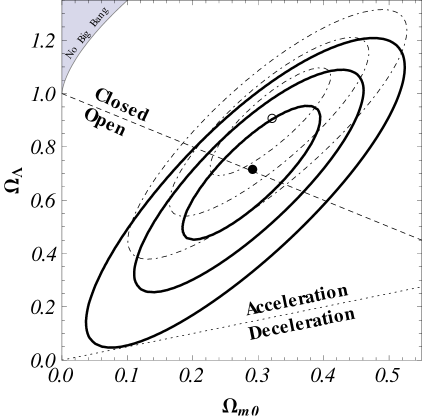
Figure 1: Solid [dot-dashed] lines show 1$\sigma$, 2$\sigma$, and 3$\sigma$ constraint contours for the $\Lambda$CDM model from the $H(z)$ data given in Table (3) for the prior $\bar{H}_{0}\pm\sigma_{H_{0}}=68\pm 2.8$ km s^-1 Mpc^-1 [$\bar{H}_{0}\pm\sigma_{H_{0}}=73.8\pm 2.4$ km s^-1 Mpc^-1]. The filled [empty] circle best-fit point is at $(\Omega_{m0},\Omega_{\Lambda})=(0.29,0.72)$ [$(0.32,0.91)$] with $\chi^{2}_{\rm min}=18.24$ [$19.30$]. The dashed diagonal line corresponds to spatially-flat models, the dotted line demarcates zero-acceleration models, and the area in the upper left-hand corner is the region for which there is no big bang. The 2 $\sigma$ intervals from the one-dimensional marginalized probability distributions are $0.15\leqslant\Omega_{m0}\leqslant 0.42$, $0.35\leqslant\Omega_{\Lambda}\leqslant 1.02$ [$0.20\leqslant\Omega_{m0}\leqslant 0.44$, $0.62\leqslant\Omega_{\Lambda}\leqslant 1.14$].

Figure 2: Solid [dot-dashed] lines show 1$\sigma$, 2$\sigma$, and 3$\sigma$ constraint contours for the XCDM parametrization from the $H(z)$ data given in Table (3) for the prior $\bar{H}_{0}\pm\sigma_{H_{0}}=68\pm 2.8$ km s^-1 Mpc^-1 [$\bar{H}_{0}\pm\sigma_{H_{0}}=73.8\pm 2.4$ km s^-1 Mpc^-1]. The filled [empty] circle is the best-fit point at $(\Omega_{m0},\omega_{X})=(0.29,-1.04)$ [$(0.26,-1.30)$] with $\chi^{2}_{\rm min}=18.18$ [$18.15$]. The dashed horizontal line at $\omega_{\rm X}=-1$ corresponds to spatially-flat $\Lambda$CDM models and the curved dotted line demarcates zero-acceleration models. The 2 $\sigma$ intervals from the one-dimensional marginalized probability distributions are $0.23\leqslant\Omega_{m0}\leqslant 0.35$, $-1.51\leqslant\omega_{X}\leqslant-0.64$ [$0.22\leqslant\Omega_{m0}\leqslant 0.31$, $-1.78\leqslant\omega_{X}\leqslant-0.92$].

Figure 3: Solid [dot-dashed] lines show 1$\sigma$, 2$\sigma$, and 3$\sigma$ constraint contours for the $\phi$CDM model from the $H(z)$ data given in Table (3) for the prior $\bar{H}_{0}\pm\sigma_{H_{0}}=68\pm 2.8$ km s^-1 Mpc^-1 [$\bar{H}_{0}\pm\sigma_{H_{0}}=73.8\pm 2.4$ km s^-1 Mpc^-1]. The filled [empty] circle best-fit point is at $(\Omega_{m0},\alpha)=(0.29,0)$ [$(0.25,0)$] with $\chi^{2}_{\rm min}=18.24$ [$20.64$]. The horizontal axis at $\alpha=0$ corresponds to spatially-flat $\Lambda$CDM models and the curved dotted line demarcates zero-acceleration models. The 2 $\sigma$ intervals from the one-dimensional marginalized probability distributions are $0.17\leqslant\Omega_{m0}\leqslant 0.34$, $\alpha\leqslant 2.2$ [$0.16\leqslant\Omega_{m0}\leqslant 0.34$, $\alpha\leqslant 0.7$].

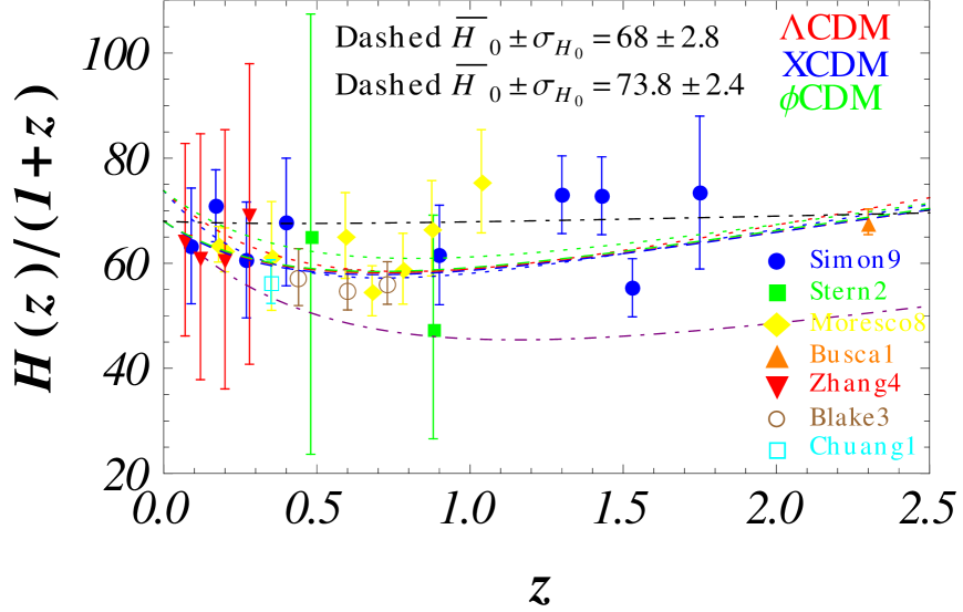
Figure 4: $H(z)/(1+z)$ data (28 points) and model predictions (lines for 6 best-fit models) as a function of redshift. The dashed [dotted] lines are for the prior $\bar{H}_{0}\pm\sigma_{H_{0}}=68\pm 2.8$ km s^-1 Mpc^-1 [$\bar{H}_{0}\pm\sigma_{H_{0}}=73.8\pm 2.4$ km s^-1 Mpc^-1], with red, blue, and green lines corresponding to the $\Lambda$CDM, XCDM, and $\phi$CDM cases. The black (purple) dot-dashed lines correspond to two models that are 3 $\sigma$ away from best-fit $\Lambda$CDM ($\phi$CDM) and have parameters $\Omega_{m}=0.04$, $\Omega_{\Lambda}=0.06$ ($\Omega_{m}=0.2$, $\alpha=0$), both for the lower value of $\bar{H}_{0}$.

Figures (1)—(3) show the constraints from the $H(z)$ data for the three dark energy models we consider, and for the two different $H_{0}$ priors. In all 6 cases the $H(z)$ data of Table 3 require accelerated cosmological expansion at the current epoch, at, or better than, 3 $\sigma$ confidence. The previous largest $H(z)$ data set used, that in Chapter (4), required this accelerated expansion at, or better than, 2 $\sigma$ confidence. Comparing Figs. (1)—(3) here to Figs. (14)—(16), we see that in the XCDM and $\phi$CDM cases the $H(z)$ data we use in this paper significantly tightens up the constraints on $w_{\rm X}$ and $\alpha$, but does not much affect the $\Omega_{m0}$ constraints. However, in the $\Lambda$CDM case the $H(z)$ data used here tightens up constraints on both $\Omega_{\Lambda}$ and $\Omega_{m0}$. We found that as we increase the value of the nuisance parameter $H_{0}$ the best-fit point for $\Lambda$CDM moves from the spatially-flat case to the closed case, and for XCDM the best-fit point moves almost orthogonally to the flat $\Lambda$CDM line, towards more negative values of $\omega_{X}$.

As indicated by the $\chi^{2}_{\rm min}$ values listed in the captions of Figs. (1)—(3), all 6 best-fit models are very consistent with the $H(z)$ data listed in Table (3). It is straightforward to compute the cosmological deceleration-acceleration transition redshift in these cases. Those are given in Table (1)

The mean and standard deviation gives $z_{\rm da}=0.74\pm 0.05$, which is in good agreement with the recent Busca et al.²⁴ determination of $z_{\rm da}=0.82\pm 0.08$ based on less data, possibly not all independent. Figure (4) shows $H(z)/(1+z)$ data from Table (3) and the 6 best-fit model predictions as a function of redshift. The deceleration-acceleration transition is not impossible to discern in the data.

Model	Prior $H_{0}$	Transition Redshift
used	(km s-1 Mpc -1)	$z_{da}$
$\Lambda$CDM	$68\pm 2.8$	0.706
	$73.8\pm 2.4$	0.785
$\Lambda$CDM	$68\pm 2.8$	0.706
	$73.8\pm 2.4$	0.785
$\Lambda$CDM	$68\pm 2.8$	0.706
	$73.8\pm 2.4$	0.785
Average		$\boldsymbol{0.74\pm 0.05}$

Table 1: Results of the transition redshifts in different models.

From Fig. 4 one sees that there are only 6 data points for $z>1$, but 22 data points for $z<1$. The larger errors of some of the $z<1$ data, as compared to those of the $z>1$ measurements, are likely responsible for the excellent reduced $\chi^{2}$ values of the best-fit models.

3 Conclusion

In summary, we have extended the analysis of Busca et al.²⁴ to a larger independent set of 28 $H(z)$ measurements and determined the cosmological deceleration-acceleration transition redshift $z_{\rm da}=0.74\pm 0.05$. These $H(z)$ data are well-described by all 6 best-fit models, and provide tight constraints on the model parameters. The $H(z)$ data require accelerated cosmological expansion at the current epoch, and are consistent with the decelerated cosmological expansion at earlier times predicted and required in standard dark energy models. While the standard spatially-flat $\Lambda$CDM model is very consistent with the $H(z)$ data, current $H(z)$ data are not able to rule out slowly evolving dark energy. More, and better quality, data are needed to better discriminate between constant and slowly-evolving dark energy density.

Chapter 6 Binned Hubble Parameter Measurements and the Cosmological Deceleration-Acceleration Transition

This chapter is based on Farooq et al.⁵⁸

1 Introduction

In the standard cosmological model dark energy dominates the current epoch energy budget, but was less important in the past when non-relativistic (cold dark and baryonic) matter dominated. The transition from non-relativistic matter dominance to dark energy dominance results in a transition from decelerated to accelerated cosmological expansion. The existence of this transition is a strong prediction of the standard cosmological model and attempts have been made to measure the transition redshift.

However, only very recently has this become possible, due to high redshift (i.e., $z$ above the deceleration-acceleration transition) data that recently became available, with the most striking being the Busca et al.²⁴ measurement of the Hubble parameter $H(z=2.3)=224\pm 8$ km s^-1 Mpc^-1, well in the matter dominated epoch of the standard $\Lambda$CDM model.

From a compilation of 28 independent $H(z)$ measurements over $0.07\leqslant z\leqslant 2.3$ Table (3), the transition redshift was found in Chapter (5) to be $z_{\rm da}=0.74\pm 0.05$. This was determined from the 6 best-fit transition redshifts measured in three different cosmological models, $\Lambda$CDM, XCDM, and $\phi$CDM, for two different Hubble constant priors.

The spatially-flat $\Lambda$CDM model¹¹⁹ is the reigning standard cosmological model. Here we consider the more general $\Lambda$CDM model that allows for non-zero space curvature. In the standard model the cosmological constant, $\Lambda$, contributes around 70$\%$ of the present cosmological energy budget, non-relativistic, pressure-less, cold dark matter (CDM) contributes a little more than 20$\%$, and non-relativistic baryonic matter makes up the remaining 5$\%$ or so. In the $\Lambda$CDM model time-independent dark energy, $\Lambda$, is modeled as a spatially homogeneous fluid with equation of state $p_{\rm\Lambda}=-\rho_{\rm\Lambda}$ where $p_{\rm\Lambda}$ and $\rho_{\rm\Lambda}$ are the fluid pressure and energy density respectively. It has been known for a while now that the spatially-flat $\Lambda$CDM model is consistent with most observational data. It is also well known that if, instead of staying constant like $\Lambda$, the dark energy density gradually decreased in time (and correspondingly slowly varied in space), it would alleviate a conceptual coincidence problem associated with the $\Lambda$CDM model.

Here we not only constraints the parameters of the two models and a dark energy parametrization, which are discussed in Chapter (2), namely non-flat $\Lambda$CDM, flat $\phi$CDM, and XCDM respectively but also find the deceleration-acceleration best-fit value of transition redshift using these models.

In addition to being affected by the cosmological model used in the analysis, the measured deceleration-acceleration transition redshift $z_{\rm da}$ depends on the assumed value of the Hubble constant. Consequently, to quantify the effect, we use two Gaussian $H_{0}$ priors in the analyses. The first prior is $\overline{H}_{0}$ $\pm$ $\sigma_{H_{0}}$ = 68 $\pm$ 2.8 km s^-1 Mpc^-1. This comes from a median statistics analysis of 553 $H_{0}$ measurements Chen et al.⁴³ and is consistent with the earlier estimates of Gott et al.⁸³ and Chen et al.⁴⁰. The second prior of $\overline{H}_{0}$ $\pm$ $\sigma_{H_{0}}$ = 73.8 $\pm$ 2.4 km s^-1 Mpc^-1 comes from recent Hubble Space Telescope measurements Riess et al.¹⁴⁵.

In Chapter (5) we determined the redshift of the deceleration-acceleration transition by finding the mean and standard deviation of the six best-fit $z_{\rm da}$ values in the 3 models (with 2 different $H_{0}$ priors). Here we use a different technique to measure $z_{\rm da}$ and the related uncertainty in each of these six cases. We then determine summary estimates of $z_{\rm da}$ by considering various weighted mean combinations of these six estimates. The transition redshifts take the forms:

$$z_{\rm da}=\left({\frac{2\Omega_{\Lambda}}{\Omega_{m0}}}\right)^{1/3}-1,$$ (1)

$$z_{\rm da}=\left({\frac{\Omega_{m0}}{(\Omega_{m0}-1)(1+3\omega_{X})}}\right)^{1/{3\omega_{X}}}-1,$$ (2)

for the $\Lambda$CDM and XCDM cases where $\Omega_{\Lambda}$ and $\Omega_{m0}$ are the cosmological constant and non-relativistic matter density parameters, and $\omega_{X}$ is the equation-of-state-parameter of dark energy. As for $\phi$CDM, from Eqs. (3) of Peebles & Ratra¹²¹ we first derive:

$$\frac{\ddot{a}}{a} = -\frac{4\pi G}{3}\left[\rho_{m}+\rho_{\phi}(1+3\omega_{\phi})\right]$$ (3)

$$= -\frac{1}{2}H_{0}^{2}\left[\Omega_{m0}(1+z)^{3}+\Omega_{\phi}(z,\alpha)(1+3\omega_{\phi}(z))\right],$$

where $\Omega_{\phi}(z)$ is the scalar field energy density parameter and:

$$\omega_{\phi}(z)=\frac{\frac{1}{2}\dot{\phi^{2}}-V(\phi)}{\frac{1}{2}\dot{\phi^{2}}+V(\phi)}.$$ (4)

The redshift $z_{\rm da}$ is determined by requiring that the right hand side of Eq. (3) vanish:

$$\Omega_{m0}(1+z_{\rm da})^{3}+\Omega_{\phi}(z_{\rm da},\alpha)\left[1+3~{}\omega_{\phi}(z_{\rm da})\right]=0.$$ (5)

To determine $z_{\rm da}$ we numerically integrate the $\phi$CDM model equations of motion, Eqs. (3) of Peebles & Ratra¹²¹, using the initial conditions described there. These solutions determine the needed functions in Eq. (5), which we then numerically solve for $z_{\rm da}(\Omega_{m0},\alpha)$.

To find the expected values $\langle z_{\rm da}\rangle$ and $\langle z_{\rm da}^{2}\rangle$ we use:

$$\langle z_{\rm da}\rangle=\frac{\iint z_{\rm da}(\textbf{p})\mathcal{L}(\textbf{p})d\textbf{p}}{\iint\mathcal{L}(\textbf{p})d\textbf{p}},~{}~{}~{}~{}~{}~{}~{}~{}~{}~{}~{}~{}\langle z_{\rm da}^{2}\rangle=\frac{\iint z_{\rm da}^{2}(\textbf{p})\mathcal{L}(\textbf{p})d\textbf{p}}{\iint\mathcal{L}(\textbf{p})d\textbf{p}}.$$ (6)

Here $\mathcal{L}(\textbf{p})$ is the $H(z)$ data likelihood function after marginalization over the $H_{0}$ prior in the model under consideration. It depends only on the model parameters $\textbf{p}=(\Omega_{m0},\Omega_{\Lambda})$ for $\Lambda$CDM, $=(\Omega_{m0},\omega_{X})$ for XCDM, and $=(\Omega_{m0},\alpha)$ for $\phi$CDM. The standard deviation in $z_{\rm da}$ is calculated from the standard formula $\sigma_{z_{\rm da}}=\sqrt{\langle z_{\rm da}^{2}\rangle-\langle z_{\rm da}\rangle^{2}}$. The results of this computation are summarized in Table (4).

It is reassuring that the results of the penultimate and the last columns of Table (4) are very consistent. In Chapter (5) we determined a summary estimate of $z_{\rm da}=0.74\pm 0.05$ by computing the mean and standard deviation of the six values in the last column of Table (4). It is of interest to estimate similar summary values for each of the two $H_{0}$ priors. We find that $z_{\rm da}=0.70\pm 0.05$ ($z_{\rm da}=0.77\pm 0.04$) for $H_{0}\pm\sigma_{H_{0}}$ = 68 $\pm$ 2.8 (73.8 $\pm$ 2.4) km s^-1 Mpc^-1. Perhaps more realistic summary estimates are determined by the weighted means of the two sets of 3 values in the penultimate column of Table (4): $z_{\rm da}=0.69\pm 0.06$ ($z_{\rm da}=0.76\pm 0.05$) for $H_{0}\pm\sigma_{H_{0}}$ = 68 $\pm$ 2.8 (73.8 $\pm$ 2.4) km s^-1 Mpc^-1, and $z_{\rm da}=0.74\pm 0.04$ are the results if all six values are used.

More conventionally, cosmological data are used to constrain model parameters values such as $\Omega_{m0}$ and $\Omega_{\Lambda}$ for the $\Lambda$CDM model. A number of different data sets have been used for this purpose. These include Type Ia supernova (SNIa) apparent magnitude verses redshift data e.g.,Ruiz et al.,¹⁴⁶ Chiba et al.,⁴⁷ Cardenas et al.,³⁴ Liao et al.,⁹⁶ Farooq et al.,⁶⁰ Campbell et al.,²⁸ cosmic microwave background (CMB) anisotropy measurements Ade et al.¹²⁸ and references therein, baryonic acoustic oscillation (BAO) peak length scale data Mehta et al.,¹¹⁰ Anderson et al.,⁴ Li et al.,⁹⁴ Scovacricchi et al.,¹⁵⁶ Farooq & Ratra⁶² and references therein, galaxy cluster gas mass fraction as a function of redshift e.g., Allen et al.,² Samushia & Ratra,¹⁵² Tong & Noh et al.,¹⁷¹ Lu et al.,¹⁰³ Solano et al.,⁵² Landry et al.,⁹² and, of special interest here, measurement of the Hubble parameter as a function of redshift Jimenezeta et al.,⁸⁶ Samushia & Ratra,¹⁵¹ Samushia et al.,¹⁵⁰ Sen et al.,¹⁵⁷ Yun & Ratra,⁴⁴ Avileset al.,¹⁰ Wang et al.,¹⁷⁸ Campos et al.,²⁹ Chimento et al.,⁴⁸ and references therein. These data, separately and in combination, provide strong evidence for accelerated cosmological expansion at the current epoch. However their error bars are still too large to allow for a discrimination between constant and time-varying dark energy densities.

Of course, both methods are equivalent, since they make use of the same data, but each has it own advantages and disadvantages. In particular, it is of some interest to actually discern the deceleration-acceleration transition in the $H(z)$ data. While the data does indicate the transition, see Fig. (4), the data points bounce around quite a bit. Given the low reduced $\chi^{2}$ for the best-fit models (see Chapter (5) and Table (4) here), all of which show significant evidence for a deceleration-acceleration transition. We investigate different data binning techniques here, to see if binned versions of the $H(z)$ measurements more clearly illustrate the presence of a deceleration-acceleration transition.

2 Binning the Data

The 28 individual $H(z)$ measurements bounce around on the $H(z)/(1+z)$ plot, Fig. 4 of Farooq & Ratra.⁶² To try to get a smoother observed $H(z)/(1+z)$ function we form bins in redshift and then combine the data points in each bin to give a single observed value of $z$, $H(z)$, and $\sigma$ for that bin. The measurements in each bin are combined using two different statistical techniques, weighted mean and median statistics.

Table (4) lists the weighted mean results. These results were computed using the standard formulae see, e.g., Podariu et al.¹³³. That is:

$$\overline{H}(z)=\frac{\sum_{i=1}^{N}H(z_{i})/\sigma_{i}^{2}}{\sum_{i=1}^{N}1/\sigma_{i}^{2}},$$ (7)

where $N$ is the number of data points in the bin under consideration, $\overline{H}(z)$ is the weighted mean of the Hubble parameter in that bin, $H(z_{i})$ is the value of the Hubble parameter measured at redshift $z_{i}$ and $\sigma_{i}$ is the corresponding uncertainty. Weighted mean redshifts, denoted by $\overline{z}$, were similarly computed:

$$\overline{z}=\frac{\sum_{i=1}^{N}z_{i}/\sigma_{i}^{2}}{\sum_{i=1}^{N}1/\sigma_{i}^{2}}.$$ (8)

The weighted mean standard deviation, denoted by $\overline{\sigma}$, for each bin was found from:

$$\overline{\sigma}=\left(\sum_{i=1}^{N}1/\sigma_{i}^{2}\right)^{-1/2}.$$ (9)

The assumptions underlying use of weighted mean statistics are that the measurement errors are Gaussian, and there are no systematic errors. Hence, one can compute $\chi^{2}$, the goodness-of-fit parameter, for each bin:

$$\chi^{2}=\frac{1}{N-1}\sum_{i=1}^{N}\frac{[H(z_{i})-\overline{H}(z)]^{2}}{\sigma_{i}^{2}},$$ (10)

which has expected value unity and error $1/\sqrt{2(N-1)}$, so we can use this to determine the number of standard deviations that $\chi$ deviates from unity for each bin:

$$N_{\overline{\sigma}}=|\chi-1|\sqrt{2(N-1)}.$$ (11)

An unaccounted for systematic error, the presence of significant correlations between the measurements, and breakdown of the Gaussian error assumption for each measurement, are the three factors that can make $N_{\overline{\sigma}}$ much greater than unity.

The second technique we use to combine measurements in a bin is median statistics, as developed in Gott et al.⁸³ Table (4) lists the median statistics results. The median is the value for which there is a $50\%$ chance of finding a measurement below or above it. It is fair to use median statistics to combine the $H(z)$ data of Table (3) since we assume that all the measurements are independent and there is no over-all systematic error in the $H(z)$ data as a whole. Individual measurements can have individual systematic errors, for discussion see Chen & Ratra. ⁴³ The median will be revealed as the true value as the number of measurements grow to infinity, and this technique reduces the effect of outliers of a set of measurements on the estimate of a true value. If $N$ measurements are considered, the probability of finding the true value between values $N_{i}$ and $N_{i+1}$ (where $i=1,2,...N$) is (see Gott et al.⁸³):

$$P_{i}=\frac{2^{-N}N!}{i!(N-1)!}$$ (12)

This process of finding a median value was used for the redshift and the Hubble parameter, and the Hubble parameter probability distribution was used to determine $\sigma$ for each bin.

We would like to have as many measurements as possible in each bin, as well as bins that are as narrow as possible in redshift space. Obviously, since these requirements are contradictory, compromise is necessary. In addition, we require roughly the same number of measurements per bin, so as to have approximately similar errors on the binned measurements. As indicated in Table (4) and Table (4) we consider four different binnings of the 23 lower redshift, $z<1.04$, measurements; the five higher redshift measurements are sparsely spread over too large a redshift range to allow for a useful binning.

The last column of Table (4) shows that the first two binnings, with approximately 3 and 5 measurements per bin, do not show any deviation from what is expected from Gaussian errors. On the other hand, the last binning, with about 8 measurements per bin, appears to be not so consistent with the assumption of Gaussian errors. This is likely a consequence of the large width in redshift of these bins, so the measurements at the low $z$ end and at the high $z$ end of each bin differ too much to be combined together. Median statistics does not make use of the error bars of the individual measurements. As a result, it is a more conservative technique, and when used to combine data in bins it results in larger error bars. A comparison of the results in Tables (4) and (4) clearly illustrates this point. Fortunately the weighted mean results we have found show that the individual lower redshift data points have reasonable error bars and so there is no obvious danger in using the more constraining weighted mean results to draw physical conclusions.

The weighted-mean and median statistics binned results of Tables (4) and (4) are plotted in the top panels of Figs. (1)—(4) (in purple). These figures also show the 5 higher $z$ unbinned measurements listed in Table (3) (in cyan). Both sets of observations show $1$ and $2$ $\sigma$ error bars. Also shown are the unbinned data (Table (3)) best-fit predictions for $\Lambda$CDM (red), XCDM (blue), and $\phi$CDM (green) for the two priors, $\overline{H}_{0}\pm\sigma_{H_{0}}$= 68 $\pm$ 2.8 km s^-1 Mpc^-1 (dashed lines) and $\overline{H}_{0}\pm\sigma_{H_{0}}$= 7.8 $\pm$ 2.4 km s^-1 Mpc^-1 (dotted lines), from Farooq & Ratra.⁶² Focusing on the weighted-mean panels in each of these plots, and comparing to Fig. (4), we see that the binned data of Figs. 1—3 clearly demarcates a declaration-acceleration transition.

3 Constraints from the binned data

In this section we use the weighted-mean and median statistics binned data to derive constraints on cosmological parameters of $\Lambda$CDM, XCDM, and $\phi$CDM, and compare these constraints to those that follow from the unbinned data of Table (3).

In order to derive constraints on the parameters p of the dark energy models discussed above, using the binned data from Tables (4) and (4), we follow the procedure of Chapter (4). The observational data consist of measurements of the Hubble parameter $H_{\rm obs}(z_{i})$ at redshifts $z_{i}$, with the corresponding one standard deviation uncertainties $\sigma_{i}$. To constrain parameters of cosmological models, we define the posterior likelihood function $\mathcal{L}_{H}(\textbf{p})$, that depends only on the model parameters p, by integrating the product of the $H_{0}$ prior likelihood function $\propto$ exp$[-(H_{0}-\bar{H}_{0})^{2}/(2\sigma^{2}_{H_{0}})]$ and the usual likelihood function exp$(-\chi_{H}^{2}/2)$, as in Eq. (18) of ⁶⁰. Two different Gaussian priors, $\overline{H}_{0}\pm\sigma_{H_{0}}$= 68 $\pm$ 2.8 km s^-1 Mpc^{-1 43} and $\overline{H}_{0}\pm\sigma_{H_{0}}$ = 73.8 $\pm$ 2.4 km s^-1 Mpc^{-1 145} are used in the marginalization of the likelihood function over the nuisance parameter $H_{0}$.

The best-fit point (BFP) $\mathbf{p_{0}}$ are those parameter values that maximize the likelihood function $\mathcal{L}_{H}(\mathbf{p})$. To find the 1, 2, and 3 $\sigma$ confidence intervals as two-dimensional parameter sets, we start from the BFP and integrate the volume under $\mathcal{L}_{H}(\mathbf{p})$ until we include 68.27, 95.45, and 99.73 % of the probability.

The lower 3 rows of panels in Figs. (1)—(4) show the constraints (1$\sigma$, 2$\sigma$, and 3$\sigma$ contours) from the unbinned $H(z)$ data of Table 1 of Farooq & Ratra,⁶² (in blue dot-dashed contours) and from the binned $H(z)$ data of Tables (4) and (4) here (in red solid contours), for the three dark energy models we consider, and for the two different $H_{0}$ priors mentioned above. The red filled circles and the blue empty circles are the best fit points for the binned and unbinned data respectively. Some relevant results are listed in Tables 4—7. Comparing the weighted-mean BFP cosmological parameter values listed in these tables, to those listed in the captions of Figs. (1)—(3), establishes the very good agreement between the values derived here using the binned data (especially for fewer measurements per bin) and the Farooq & Ratra,⁶² values derived using the unbinned data.

It is clear from the left two columns of the lower three rows of Figs. (1)—(4) that the weighted-mean binning of the first 23 data points in Table (3) give almost exactly the same constraints on model parameters p for the three cosmological models as do the unbinned data of Table (3). Since the weighted-mean technique assumes that the error in the measurements has a Gaussian distribution and that the measurements are uncorrelated, this result is consistant with this assumption that the $H(z)$ data in Table (3) have Gaussian errors. Consequently, the best way to combine the measurements in a bin is to use the weighted-mean method. It is also useful to note that when there are fewer data points in a narrower bin, the constraints from the binned data matches better with the constraints derived from the unbinned data. This is not unexpected. In the case of median statistics, however, the constraints on model parameters for all three models from the binned data are much less restrictive than those derived from the unbinned data, see the right hand column of panels in the lower three rows of Figs (1)—(4). This is because median statistics is a more conservative technique and so, in this case, is not the best way of combining $H(z)$ measurements in bins. It is also interesting to note, from Tables (1)—(4), that $\chi^{2}_{\rm min}$ for the case of median statistics is significantly smaller than $\chi^{2}_{\rm min}$ for the weighted mean case. This is a direct consequence of the larger error bars estimated by the more conservative median statistics approach.

4 Conclusion

We have shown that the weighted-mean combinations of the lower redshift $H(z)$ measurements by bins in redshift provide close to identical constraints on cosmological model parameters as do the unbinned $H(z)$ data tabulated in Farooq & Ratra.⁶² This is consistent with the $H(z)$ measurements errors being Gaussian.

When plotted against $z$, the weighted-mean binned $H(z)/(1+z)$ measurements bounce around much less than the individual measurements considered in Farooq & Ratra,⁶² and now much more clearly show the presence of a cosmological deceleration-acceleration transition, consistent with the new summary redshift $z_{\rm da}=0.74\pm 0.04$ estimated here and consistent with that estimated in Farooq & Ratra,⁶² This result is also consistent with what is expected in the standard spatially-flat $\Lambda$CDM model, and in other cosmological models with present-epoch energy budget dominated by dark energy.

More, and more precise, measurements of $H(z)$ in the redshift range $1\lesssim z\lesssim 2.5$ will allow for a clearer demarcation of the cosmological deceleration-acceleration transition. We anticipate that such data will soon become available.

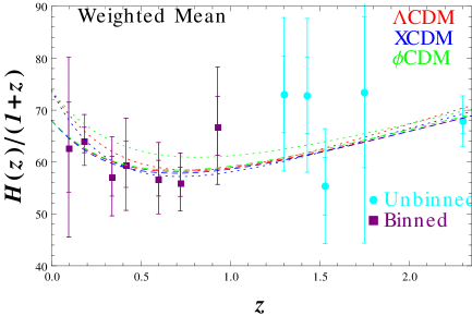
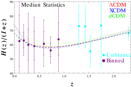
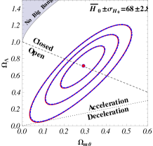
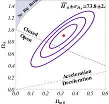
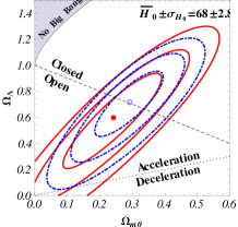
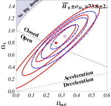
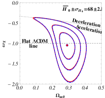
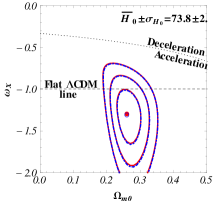
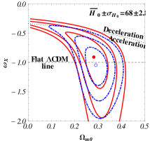
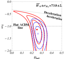
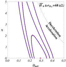
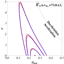
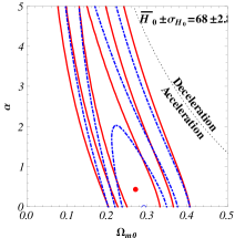
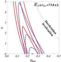
Figure 1: Top left (right) panel shows the $H(z)/(1+z)$ data, binned with 3 or 4 measurements per bin, as well as 5 higher $z$ measurements, and the Farooq & Ratra⁶² best-fit model predictions, dashed (dotted) for lower (higher) $H_{0}$ prior. The 2nd through 4th rows show the $H(z)$ constraints for $\Lambda$CDM, XCDM, and $\phi$CDM. Red (blue dot-dashed) contours are 1$\sigma$, 2$\sigma$, and 3$\sigma$ confidence interval results from 3 or 4 measurements per bin (unbinned Table (3)) data. In these three rows, the first two plots include red weighted-mean constraints while the second two include red median statistics ones. The filled red (empty blue) circle is the corresponding best-fit point. Dashed diagonal lines show spatially-flat models, and dotted lines indicate zero-acceleration models. For quantitative details see Table (1).

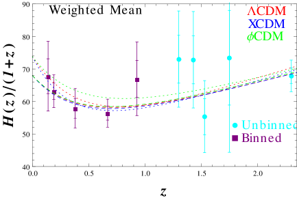
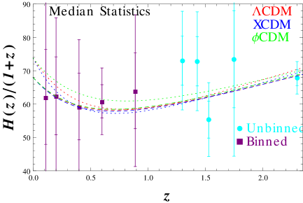
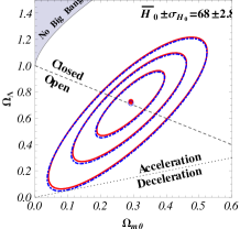
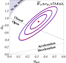
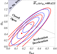
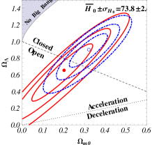
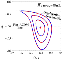
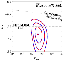
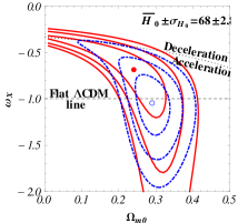
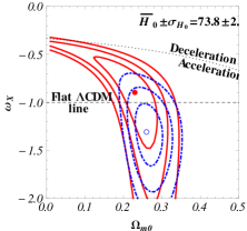
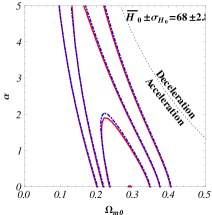
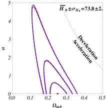
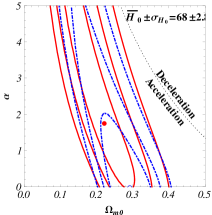
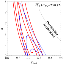
Figure 2: Top left (right) panel shows the $H(z)/(1+z)$ data, binned with 4 or 5 measurements per bin, as well as 5 higher $z$ measurements, and the Farooq & Ratra⁶² best-fit model predictions, dashed (dotted) for lower (higher) $H_{0}$ prior. The 2nd through 4th rows show the $H(z)$ constraints for $\Lambda$CDM, XCDM, and $\phi$CDM. Red (blue dot-dashed) contours are 1$\sigma$, 2$\sigma$, and 3$\sigma$ confidence interval results from 4 or 5 measurements per bin (unbinned Farooq & Ratra,⁶² Table 1) data. In these three rows, the first two plots include red weighted-mean constraints while the second two include red median statistics ones. The filled red (empty blue) circle is the corresponding best-fit point. Dashed diagonal lines show spatially-flat models, and dotted lines indicate zero-acceleration models. For quantitative details see Table (2).

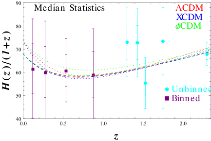
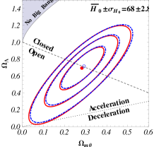
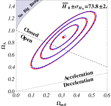
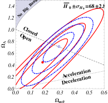
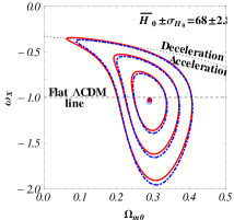
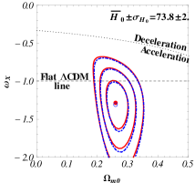
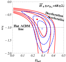
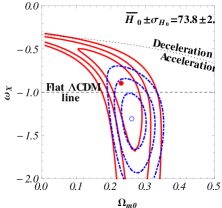
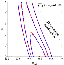
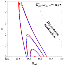
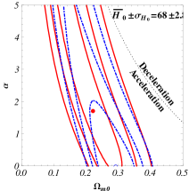
Figure 3: Top left (right) panel shows the $H(z)/(1+z)$ data, binned with 5 or 6 measurements per bin, as well as 5 higher $z$ measurements, and the Farooq & Ratra⁶² best-fit model predictions, dashed (dotted) for lower (higher) $H_{0}$ prior. The 2nd through 4th rows show the $H(z)$ constraints for $\Lambda$CDM, XCDM, and $\phi$CDM. Red (blue dot-dashed) contours are 1$\sigma$, 2$\sigma$, and 3$\sigma$ confidence interval results from 5 or 6 measurements per bin (unbinned Farooq & Ratra,⁶² Table 1) data. In these three rows, the first two plots include red weighted-mean constraints while the second two include red median statistics ones. The filled red (empty blue) circle is the corresponding best-fit point. Dashed diagonal lines show spatially-flat models, and dotted lines indicate zero-acceleration models. For quantitative details see Table (3).

[h!] Deceleration-Acceleration Transition Redshifts^a $h$ Prior^b Best-Fit Values $\chi_{\rm min}^{2}$ $z_{da}\pm\sigma_{z_{da}}$^c $z_{da}$^d $\Lambda$CDM 0.68 $\pm$ 0.028 $(\Omega_{m0},\Omega_{\Lambda})=(0.29,0.72)$ 18.2 0.690 $\pm$ 0.096 0.706 0.738 $\pm$ 0.024 $(\Omega_{m0},\Omega_{\Lambda})=(0.32,0.91$) 19.3 0.781 $\pm$ 0.067 0.785 XCDM 0.68 $\pm$ 0.028 $(\Omega_{m0},\omega_{X})=(0.29,-1.04)$ 18.2 0.677 $\pm$ 0.097 0.695 0.738 $\pm$ 0.024 $(\Omega_{m0},\omega_{X})=(0.26,-1.30)$ 18.2 0.696 $\pm$ 0.082 0.718 $\phi$CDM 0.68 $\pm$ 0.028 $(\Omega_{m0},\alpha)=(0.29,0.00)$ 18.2 0.724 $\pm$ 0.148 0.698 0.738 $\pm$ 0.024 $(\Omega_{m0},\alpha)=(0.25,0.00)$ 20.7 0.850 $\pm$ 0.116 0.817

• Estimated using the unbinned data in Table (3).

• Hubble constant in units of 100 km s^-1 Mpc^-1.

• Computed using Eqs. (1)—(6).

• The deceleration-acceleration transition redshift in the model with the best-fit values of the cosmological parameters, as computed in Farooq & Ratra⁶².

[h!] Weighted Mean Results For 23 Lower Redshift Measurements Bin $N$ $z{\textsuperscript{a}}$ $H(z)$ $H(z)$ (1 $\sigma$ range) $H(z)$ (2 $\sigma$ range) $N_{\sigma}$ (km s^-1 Mpc ^-1) (km s^-1 Mpc ^-1) (km s^-1 Mpc ^-1) 3 or 4 measurements per bin 1 3 0.096 69.0 59.4$-$78.5 49.9$-$88.0 2.00 2 4 0.185 76.0 73.1$-$78.9 70.2$-$81.8 1.73 3 3 0.338 76.6 71.5$-$81.8 66.4$-$86.9 1.89 4 3 0.417 84.4 78.1$-$90.7 71.8$-$97.0 1.55 5 3 0.598 90.9 85.4$-$96.4 79.9$-$102 0.73 6 3 0.720 96.6 91.8$-$101 87.0$-$106 1.17 7 4 0.929 129 118$-$140 107$-$151 0.13 4 or 5 measurements per bin 1 4 0.139 77.2 71.1$-$83.3 64.9$-$89.5 1.41 2 5 0.191 75.2 72.1$-$78.2 69.1$-$81.2 2.71 3 5 0.380 79.9 75.8$-$84.1 71.6$-$88.3 1.81 4 5 0.668 94.1 90.5$-$97.7 86.8$-$101 0.91 5 4 0.929 129 118$-$140 107$-$151 0.13 5 or 6 measurements per bin 1 5 0.167 75.7 72.3$-$79.0 69.0$-$82.3 1.86 2 6 0.271 76.2 72.7$-$79.7 69.3$-$83.1 2.89 3 6 0.569 89.4 85.5$-$93.2 81.7$-$97.0 1.70 4 6 0.787 106 101$-$112 95.8$-$117 2.50 7 or 9 measurements per bin 1 7 0.177 75.4 72.7$-$78.2 69.9$-$81.0 2.66 2 9 0.448 83.6 80.3$-$86.8 77.1$-$90.0 1.29 3 7 0.754 102 97.6$-$106 93.2$-$111 2.99

• Weighted mean of $z$ values of measurements in the bin.

[h!] Median Statistics Results For 23 Lower Redshift Measurements Bin $N$ $z{\textsuperscript{a}}$ $H(z)$ $H(z)$ (1 $\sigma$ range) $H(z)$ (2 $\sigma$ range) (km s^-1 Mpc ^-1) (km s^-1 Mpc ^-1) (km s^-1 Mpc ^-1) 3 or 4 measurements per bin 1 3 0.100 69.0 49.4$-$88.6 29.8$-$108 2 4 0.189 75.0 68.5$-$81.5 62.0$-$88.0 3 3 0.280 77.0 63.0$-$91.0 49.0$-$105 4 3 0.400 83.0 69.0$-$97.0 55.0$-$111 5 3 0.593 97.0 84.0$-$110 71.0$-$123 6 3 0.730 97.3 89.3$-$105 81.3$-$113 7 4 0.890 121 99.5$-$143 78.0$-$164 4 or 5 measurements per bin 1 4 0.110 69.0 53.2$-$84.8 37.4$-$101 2 5 0.200 75.0 61.0$-$89.0 47.0$-$103 3 5 0.400 83.0 69.0$-$97.0 55.0$-$111 4 5 0.680 97.3 89.3$-$105 81.3$-$113 5 4 0.890 121 99.5$-$143 78.0$-$164 5 or 6 measurements per bin 1 5 0.120 69.0 57.0$-$81.0 45.0$-$93.0 2 6 0.275 76.7 62.7$-$90.7 48.7$-$105 3 6 0.537 93.5 83.0$-$104 72.5$-$115 4 6 0.878 111 92.5$-$130 74.0$-$148 7 or 9 measurements per bin 1 7 0.170 72.9 60.9$-$84.9 48.9$-$96.9 2 9 0.400 87.9 73.9$-$102 59.9$-$116 3 7 0.875 105 88.0$-$122 71.0$-$139

• Median of $z$ values of measurements in the bin.

Table 1: Best-Fit Points And Minimum $\chi^{2}$s For 3 Or 4 Measurements Per Bin

		Weighted Mean		Median
Model	$h$ Prior	BFP	$\chi^{2}_{\rm min}$	BFP	$\chi^{2}_{\rm min}$
$\Lambda$CDM	$0.68\pm 0.028$	$\Omega_{m0}=0.29$	13.0	$\Omega_{m0}=0.24$	8.75
		$\Omega_{\Lambda}=0.72$		$\Omega_{\Lambda}=0.60$
	$0.738\pm 0.024$	$\Omega_{m0}=0.32$	14.1	$\Omega_{m0}=0.26$	9.37
		$\Omega_{\Lambda}=0.91$		$\Omega_{\Lambda}=0.80$
XCDM	$0.68\pm 0.028$	$\Omega_{m0}=0.29$	13.0	$\Omega_{m0}=0.28$	8.85
		$\omega_{X}=-1.04$		$\omega_{X}=-0.90$
	$0.738\pm 0.024$	$\Omega_{m0}=0.26$	13.0	$\Omega_{m0}=0.25$	9.18
		$\omega_{X}=-1.29$		$\omega_{X}=-1.13$
$\phi$CDM	$0.68\pm 0.028$	$\Omega_{m0}=0.29$	13.0	$\Omega_{m0}=0.27$	8.82
		$\alpha=0.00$		$\alpha=0.46$
	$0.738\pm 0.024$	$\Omega_{m0}=0.25$	15.4	$\Omega_{m0}=0.24$	9.43
		$\alpha=0.00$		$\alpha=0.00$

Table 2: Best-Fit Points And Minimum $\chi^{2}$s For 4 Or 5 Measurements Per Bin

		Weighted Mean		Median
Model	$h$ Prior	BFP	$\chi^{2}_{\rm min}$	BFP	$\chi^{2}_{\rm min}$
$\Lambda$CDM	$0.68\pm 0.028$	$\Omega_{m0}=0.29$	12.9	$\Omega_{m0}=0.17$	7.62
		$\Omega_{\Lambda}=0.73$		$\Omega_{\Lambda}=0.43$
	$0.738\pm 0.024$	$\Omega_{m0}=0.32$	13.7	$\Omega_{m0}=0.20$	8.04
		$\Omega_{\Lambda}=0.91$		$\Omega_{\Lambda}=0.66$
XCDM	$0.68\pm 0.028$	$\Omega_{m0}=0.29$	12.9	$\Omega_{m0}=0.24$	7.75
		$\omega_{X}=-1.06$		$\omega_{X}=-0.68$
	$0.738\pm 0.024$	$\Omega_{m0}=0.26$	12.5	$\Omega_{m0}=0.23$	8.17
		$\omega_{X}=-1.31$		$\omega_{X}=-0.89$
$\phi$CDM	$0.68\pm 0.028$	$\Omega_{m0}=0.29$	13.0	$\Omega_{m0}=0.22$	7.70
		$\alpha=0.00$		$\alpha=1.77$
	$0.738\pm 0.024$	$\Omega_{m0}=0.25$	15.2	$\Omega_{m0}=0.23$	8.13
		$\alpha=0.00$		$\alpha=0.30$

Table 3: Best-Fit Points And Minimum $\chi^{2}$s For 5 Or 6 Measurements Per Bin

		Weighted Mean		Median
Model	$h$ Prior	BFP	$\chi^{2}_{\rm min}$	BFP	$\chi^{2}_{\rm min}$
$\Lambda$CDM	$0.68\pm 0.028$	$\Omega_{m0}=0.28$	10.2	$\Omega_{m0}=0.18$	7.65
		$\Omega_{\Lambda}=0.70$		$\Omega_{\Lambda}=0.45$
	$0.738\pm 0.024$	$\Omega_{m0}=0.31$	11.2	$\Omega_{m0}=0.20$	8.13
		$\Omega_{\Lambda}=0.89$		$\Omega_{\Lambda}=0.66$
XCDM	$0.68\pm 0.028$	$\Omega_{m0}=0.29$	10.2	$\Omega_{m0}=0.24$	7.77
		$\omega_{X}=-1.01$		$\omega_{X}=-0.68$
	$0.738\pm 0.024$	$\Omega_{m0}=0.26$	10.2	$\Omega_{m0}=0.23$	8.25
		$\omega_{X}=-1.28$		$\omega_{X}=-0.89$
$\phi$CDM	$0.68\pm 0.028$	$\Omega_{m0}=0.29$	10.2	$\Omega_{m0}=0.22$	7.72
		$\alpha=0.00$		$\alpha=1.73$
	$0.738\pm 0.024$	$\Omega_{m0}=0.25$	12.4	$\Omega_{m0}=0.23$	8.21
		$\alpha=0.00$		$\alpha=0.30$

Table 4: Best-Fit Points And Minimum $\chi^{2}$s For 7 Or 9 Measurements Per Bin

		Weighted Mean		Median
Model	$h$ Prior	BFP	$\chi^{2}_{\rm min}$	BFP	$\chi^{2}_{\rm min}$
$\Lambda$CDM	$0.68\pm 0.028$	$\Omega_{m0}=0.29$	9.7	$\Omega_{m0}=0.17$	7.76
		$\Omega_{\Lambda}=0.73$		$\Omega_{\Lambda}=0.43$
	$0.738\pm 0.024$	$\Omega_{m0}=0.31$	10.4	$\Omega_{m0}=0.19$	7.88
		$\Omega_{\Lambda}=0.90$		$\Omega_{\Lambda}=0.64$
XCDM	$0.68\pm 0.028$	$\Omega_{m0}=0.29$	9.7	$\Omega_{m0}=0.24$	7.82
		$\omega_{X}=-1.04$		$\omega_{X}=-0.69$
	$0.738\pm 0.024$	$\Omega_{m0}=0.26$	9.5	$\Omega_{m0}=0.23$	7.97
		$\omega_{X}=-1.28$		$\omega_{X}=-0.90$
$\phi$CDM	$0.68\pm 0.028$	$\Omega_{m0}=0.28$	9.7	$\Omega_{m0}=0.22$	7.80
		$\alpha=0.00$		$\alpha=1.69$
	$0.738\pm 0.024$	$\Omega_{m0}=0.25$	11.8	$\Omega_{m0}=0.22$	7.93
		$\alpha=0.00$		$\alpha=0.48$

Chapter 7 Observational Constraints on Non-Flat Dynamical Dark Energy Cosmological Models

This chapter is based on Farooq et al.⁵⁹

We constrain two non-flat time-evolving dark energy cosmological models by using Hubble parameter data, Type Ia supernova apparent magnitude measurements, and baryonic acoustic oscillation peak length scale observations. The inclusion of space curvature as a free parameter in the analysis results in a significant broadening of the allowed range of values of the parameter that governs the time evolution of the dark energy density in these models. While consistent with the “standard” spatially-flat $\Lambda$CDM cosmological model, these data are also consistent with a range of mildly non-flat, slowly time-varying dark energy models. After marginalizing over all other parameters, these data require the averaged magnitude of the curvature density parameter $|\Omega_{k0}|\lesssim 0.15$ at 1$\sigma$ confidence.

1 Introduction

There is significant observational evidence that the Universe is currently undergoing accelerated expansion. Most cosmologists believe that dark energy dominates the current cosmological energy budget and is responsible for this accelerated expansion (for reviews of dark energy see Li et al.,⁹⁵ Tsujikawa,¹⁷⁵ Solà,¹⁶² and references therein). In addition, if one assumes that the dark energy density is close to or time independent, cosmic microwave background (CMB) anisotropy measurements indicate that the Universe must be close to or spatially flat (Ade et al.,¹²⁸ and references therein; for an early indication see Podariu et al.,¹³³). Conversely, if one assumes that the space sections are flat, the data favor a time-independent cosmological constant. However, as far as we are aware, there has not been an analysis of observational data based on a consistent non-spatially-flat dynamical dark energy model. In this chapter we present the first such analysis.

As a warm-up exercise, we consider the popular XCDM parameterization of dynamical dark energy. The XCDM parameterization is a generalization of the standard $\Lambda$CDM cosmological model from Peebles.¹¹⁹ In the $\Lambda$CDM, case the current energy budget is dominated by a time-independent cosmological constant $\Lambda$. It is well-known that the $\Lambda$CDM model has some puzzling features which are more easily understood if, instead of remaining constant like $\Lambda$, the dark energy density gradually decreases with time.

The simplest, complete and consistent time-varying dark energy model is $\phi$CDM (see Peebles & Ratra,¹²¹ and Ratra & Peebles,¹³⁹ for detail). Here the dark energy is modeled as a scalar field, $\phi$, with a gradually decreasing (in $\phi$) potential energy density $V(\phi)$. In this paper we assume an inverse-power-law potential energy density, $V(\phi)\propto\phi^{-\alpha}$, where $\alpha$ is a nonnegative constant Peebles & Ratra.¹²¹ At $\alpha=0$ the $\phi$CDM model reduces to the corresponding $\Lambda$CDM case. The $\phi$CDM model was originally formulated in a spatially-flat cosmological model. In this chapter we consider the ¹¹⁷ generalization of the $\phi$CDM model to non-flat space.

For some time now, most observational constraints have been reasonably consistent with the predictions of the “standard” spatially-flat $\Lambda$CDM model for early indications see e.g., ⁸⁵, ¹⁸⁵, ⁵³, ². The big four, CMB anisotropy e.g., Plank results¹²⁸, supernova Type Ia (SNIa) apparent magnitude versus redshift e.g., Suzuki et al.,¹⁶⁸ Salzano et al.,¹⁴⁸ Campbell et al.,²⁸ baryonic acoustic oscillation (BAO) peak length scale e.g., ¹²³, ¹⁵, ¹⁹, ¹¹⁰, and Hubble parameter as a function of redshift e.g., ⁴⁴, ¹¹², ²⁴, ⁶² measurements provide the strongest support for this conclusion.

Other measurements that have been used to constrain cosmological parameters include, for example, galaxy cluster gas mass fraction as a function of redshift e.g., Allen et al.,² Samushia & Ratra,¹⁵² Tong et al.,¹⁷¹ Lu et al.,¹⁰³ Landry et al.,⁹² galaxy cluster and other large-scale structure properties Mortonson et al.,¹¹³ Devi et al.,³⁸ Wang,¹⁸⁰ De Boni et al.,⁵⁴ Batista et al.,¹³ and references therein, gamma-ray burst luminosity distance as a function of redshift e.g., Samushia & Ratra, ¹⁵³ Wang & Dai,¹⁷⁷ Busti et al.,²⁵ Pan et al.¹¹⁶, HII starburst galaxy apparent magnitude as a function of redshift e.g., Plionis et al.,^{129, 130} Mania & Ratra,¹⁰⁷, angular size as a function of redshift e.g., Guerra et al.,⁷⁵ Bonamente et al.,²¹ Chen & Ratra,⁴⁶, and strong gravitational lensing Chae et al.,³⁷ Lee & Ng,⁹³ Biesiada et al.,¹⁷ Suyu et al.,¹⁶⁷ and references therein. While the constraints from these data are typically less restrictive than those derived from the $H(z)$, SNIa, CMB anisotropy, and BAO data, both types of measurements result in largely compatible constraints that generally support a currently accelerating cosmological expansion. This provides confidence that the broad outlines of a “standard” cosmological model are now in place.

In this chapter we consider an extension of this “standard” cosmological model by allowing for the possibility of non-zero space curvature. As mentioned above we consider two possibilities, a generalization of the XCDM parameterization as well as the Pavlov et al.¹¹⁷ generalization of the $\phi$CDM model. In this chapter we derive constraints on the parameters of these options by using $H(z)$, SNIa, and BAO data.

Here, we do not make use of the last of the big four data, that of CMB anisotropy. While these data are widely credited with providing the strongest evidence for a very small contribution to the current energy budget from spatial curvature (see discussion above), it is not straightforward to include them in the analyses because they require an analysis of the evolution of spatial inhomogeneities. In the case of the XCDM parametrization this is not possible without an additional ad hoc extension. In the $\phi$CDM case this requires a detailed computation, including the assumption of an early epoch of inflation in non-flat space and a derivation of the concomitant power spectrum needed for the CMB anisotropy computation. It is well known that the CMB anisotropy is almost certainly a consequence of quantum-mechanical zero-point fluctuations generated during inflation see e.g., ⁶⁶, ¹⁴¹. While conceptually similar, the computation of the primordial spectrum is somewhat more involved in the spatially curved case see e.g., ^{72, 140, 142, 88, 23, 105, 187, 68, 78}. Consequently, the computation of CMB anisotropy constraints is beyond the scope of this initial paper. Even though we do not use CMB anisotropy constraints here, a combination of the other three of the big four data— $H(z)$, SNIa, and BAO— results in reasonably tight constraints on space curvature. For technical computational reasons we believe our XCDM parametrization constraints are more reflective of the true constraints on space curvature. In the XCDM case, marginalizing over all other parameters, the $H(z)$, SNIa, and BAO data require $|\Omega_{k0}|\leq 0.15$ and 0.3 at about 1$\sigma$ and 2$\sigma$ confidence.

2 Time Varying Dark Energy Models in Curved Space

In this section we summarize the two models we constrain. These are the ¹¹⁷ generalization to curved space of the time-evolving dark energy $\phi$CDM model ¹²¹, ¹³⁹, as well as the curved space generalization of the widely-used XCDM dynamic dark energy parameterization in which dark energy is modeled as a spatially-homogeneous time-dependent $X$-fluid.

We assume that general relativity provides an accurate description of gravitation on cosmological scales. The equations of motion are Einstein’s field equations,

$$R_{\mu\nu}-\frac{1}{2}Rg_{\mu\nu}=8\pi GT_{\mu\nu}-\Lambda g_{\mu\nu}.$$ (1)

Here $R_{\mu\nu}$ and $R$ are the Ricci tensor and scalar, $g_{\mu\nu}$ is the metric tensor, $\Lambda$ is the cosmological constant, $T_{\mu\nu}$ is the energy-momentum tensor of the matter present, and $G$ is the Newtonian gravitational constant.

At late times, we can ignore radiation and model non-relativistic (cold dark and baryonic) matter as a perfect fluid with energy-momentum tensor $T_{\mu\nu}={\rm diag}(\rho,p,p,p)$ where $\rho$ and $p$ are the energy density and the pressure of the fluid. Assuming the cosmological principle of spatial homogeneity, Einstein’s equations reduce to the two independent Friedmann equations:

$$\left(\frac{\dot{a}}{a}\right)^{2}=\frac{8\pi G}{3}\rho-\frac{k}{a^{2}}+\frac{\Lambda}{3},$$ (2)

$$\hskip 28.45274pt\frac{\ddot{a}}{a}\ \ =-\frac{4\pi G}{3}(\rho+3p)+\frac{\Lambda}{3}.$$ (3)

Here, $a(t)$ is the cosmological scale factor which is the ratio of the physical distance to the co-moving distance of a sufficiently distant object (so that the spatial homogeneity assumption is valid), an overdot denotes a derivative with respect to cosmological time, $k$ represents the curvature of spatial hypersurfaces (and can have three discrete values $-1$, $0$, or $+1$, corresponding to hyperbolic, flat, and spherical geometry respectively), and $\rho$ and $p$ are the sums of all (time-dependent) densities and pressures of the various forms of matter present.

With a single type of matter, the Friedmann equations (2)—(3) are two equations with three time-dependent unknowns: $a(t)$, $\rho(t)$, and $p(t)$. We can complete the system of equations with an equation of state for each type of matter. This is a relation between pressure and energy density for each type of matter:

$$p=p(\rho)=\omega\rho,$$ (4)

where $\omega$ is the dimensionless equation-of-state parameter. For non-relativistic matter $\omega=0$, while $\omega=-1$ corresponds to a standard cosmological constant $\Lambda$, and $\omega<-1/3$ corresponds to the XCDM parameterization.

Equations (2)—(4) form a closed set and can be used to derive the energy conservation equation:

$$\frac{\dot{\rho}}{\rho}=-3\ \frac{\dot{a}}{a}\ (1+\omega).$$ (5)

This first-order linear differential equation can be solved with the boundary condition $\rho(t_{0})=\rho_{0}$, where $t_{0}$ is the current time and $\rho_{0}$ is the current value of the energy density of the particular type of matter under consideration. The solution is:

$$\rho(t)=\rho_{0}\left(\frac{a_{0}}{a}\right)^{3(1+\omega)},$$ (6)

where $a_{0}$ is the current value of the scale factor. If there are a number of different species of non-interacting fluids, then Eq. (6) holds separately for each of them with the corresponding $\omega$ and $\rho_{0}$. For a non-relativistic gas (cold matter) $\omega=\omega_{m}=0$ and $\rho_{m}\propto a^{-3}$, for a homogeneous $X$-fluid $\omega=\omega_{X}<-1/3$ and $\rho_{X}\propto a^{-3(1+\omega_{X})}$, and for spatial curvature $\omega=\omega_{k}=-1/3$ and $\rho_{k}\propto a^{-2}$.

The ratio $\dot{a}(t)/a(t)$ in Eq. (2) is the Hubble parameter $H(t)$. The present value of the Hubble parameter is the Hubble constant $H_{0}$. To rewrite the Friedmann equation (2) in terms of observable parameters, we define the dimensionless redshift $z=a_{0}/a-1$ and the present value of the density parameters:

$$\Omega_{m0}=\frac{8\pi G\rho_{m0}}{3H_{0}^{2}},\ \ \ \ \ \ \ \Omega_{k0}=\frac{-k}{(H_{0}a_{0})^{2}},\ \ \ \ \ \ \ \Omega_{X0}=\frac{8\pi G\rho_{X0}}{3H_{0}^{2}}.$$ (7)

Here we have parameterized dark energy as a spatially homogeneous $X$-fluid with current density parameter value $\Omega_{X0}$, $\Omega_{m0}$ is the current non-relativistic (baryonic and cold dark) matter density parameter, and $\Omega_{k0}$ is that of spatial curvature (with $\Omega_{k0}>0$ corresponding to an open or hyperbolic spatial geometry). With these definitions Eq. (2) becomes:

$$H^{2}(z;H_{0},\textbf{p}) = H_{0}^{2}\left[\Omega_{m0}(1+z)^{3}+(1-\Omega_{m0}-\Omega_{k0})(1+z)^{3(1+\omega_{X})}+\Omega_{k0}(1+z)^{2}\right],$$ (8)

where we have made use of $\Omega_{X0}=1-\Omega_{m0}-\Omega_{k0}$. This is the Friedmann equation for the XCDM parameterization with non-zero spatial curvature. In this case, the cosmological parameters are taken to be $\textbf{p}=({\Omega_{m0},\omega_{X},\Omega_{k0}})$. The XCDM parameterization is incomplete, as it cannot describe the evolution of energy density inhomogeneities see e.g. Ratra,¹³⁸ and Podariu et al.¹³²

The second model we consider is the simplest, complete and consistent dynamical dark energy model, $\phi$CDM, generalized to include non-zero spatial curvature Pavlov et al.¹¹⁷ In this case, dark energy is modeled as a slowly-rolling scalar field $\phi$ with an, e.g., inverse-power-law potential energy density $V(\phi)=\kappa m_{p}^{2}\phi^{-\alpha}/2$ where $m_{p}=1/\sqrt{G}$ is the Planck mass and $\alpha$ is a non-negative parameter that determines the coefficient $\kappa$.¹²¹ The scalar field part of the $\phi$CDM model action is:

$$S=\frac{m_{p}^{2}}{32\pi}\int{\sqrt{-g}\left(~{}g^{\mu\nu}\partial_{\mu}\phi\partial_{\nu}\phi-\kappa m_{p}^{2}\phi^{-\alpha}\right)d^{4}x},$$ (9)

where the parameter $\kappa$ is: ¹²¹, ¹¹⁷

$$\kappa=\frac{8}{3}\left(\frac{2\alpha}{3}\right)^{\alpha/2}(\alpha+4)(\alpha+2)^{(\alpha-2)/2}.$$ (10)

In this model, at the current epoch, scalar field dark energy dominates the cosmological energy budget and fuels the accelerating cosmological expansion. Prior to that, space curvature dominated and at even earlier times, non-relativistic matter powered the decelerating cosmological expansion. In the matter dominated epoch at $a\ll a_{0}$, $\rho_{\phi}\ll\rho_{m}$ and $\rho_{k}\ll\rho_{m}$, the Einstein-de Sitter model applies, and the initial conditions are that the cosmological scale factor evolves as $a(t)\propto t^{2/3}$, the scalar field $\phi(t)\propto t^{2/(\alpha+2)}$, and the scalar field energy density evolves as $\rho_{\phi}\propto a^{-3\alpha/(\alpha+2)}\propto t^{-2\alpha/(\alpha+2)}$, as described in ¹²¹. In the space curvature dominated epoch $\rho_{\phi}\ll\rho_{k}$ and $\rho_{m}\ll\rho_{k}$ and $a(t)\propto t$, the scalar field $\phi(t)\propto t^{2/(2+\alpha)}$, and the scalar field energy density evolves as $\rho_{\phi}\propto a^{-2\alpha/(2+\alpha)}\propto t^{-2\alpha/(2+\alpha)}$, as determined in Pavlov et al.¹¹⁷ Hence, for positive values of $\alpha$, the scalar field energy decreases, but less rapidly than that of space curvature in the space curvature dominated epoch ($\rho_{k}\propto a^{-2}\propto t^{-2}$) and less rapidly than that of non-relativistic matter in the matter dominated epoch ($\rho_{m}\propto a^{-3}\propto t^{-2}$). So at late times the Universe will become dark energy dominated ¹¹⁷, ¹³⁹. As in the radiation and matter dominated epochs, Peebles & Ratra,¹²¹ Ratra & Peebles,¹³⁹ and Pavlov et al.,¹¹⁷ show that in the curvature dominated epoch the solution for the scalar field is a time-dependent fixed point or attractor. This means that for a wide range of initial conditions the solution will approach this special time-dependent fixed point solution.

The equation of motion of the scalar field is:

$$\ddot{\phi}+3\frac{\dot{a}}{a}\dot{\phi}-\frac{1}{2}\kappa\alpha m_{p}^{2}\phi^{-(\alpha+1)}=0.$$ (11)

In the presence of spatial curvature the $\phi$CDM model Friedmann equation takes the form:

$$H^{2}(z;H_{0},\textbf{p}) = H_{0}^{2}[\Omega_{m0}(1+z)^{3}+\Omega_{\phi}(z,\alpha)+\Omega_{k0}(1+z)^{2}],$$ (12)

where the time-dependent scalar field density parameter $\Omega_{\phi}$ is defined as:

$$\Omega_{\phi}(z,\alpha)\equiv\frac{8\pi G}{3H^{2}_{0}}\rho_{\phi}=\frac{1}{12H^{2}_{0}}\left(\dot{\phi}^{2}+\kappa m^{2}_{p}\phi^{-\alpha}\right).$$ (13)

In the limit $\alpha=0$, the $\phi$CDM model is equivalent to the ordinary time-independent cosmological constant $\Lambda$ model. This makes the $\phi$CDM model a generalization of the standard $\Lambda$CDM model of cosmology.

Solving the coupled differential equations (11)—(13), with the initial conditions described in Peebles & Ratra,¹²¹ and Pavlov et al.,¹¹⁷ allows for a numerical computation of the Hubble parameter $H(z;H_{0},\textbf{p})$, as well as the other functions needed for applications of the cosmological tests. In this case the model parameters are taken to be $\textbf{p}=(\Omega_{m0},\alpha,\Omega_{k0})$.

3 Observational Constraints

To constrain cosmological parameters p, we generalize the technique described in Farooq & Ratra,⁶¹ to models with three free parameters, $\textbf{p}=(\Omega_{m0},\omega_{X},\Omega_{k0})$ for the XCDM parameterization and $\textbf{p}=(\Omega_{m0},\alpha,\Omega_{k0})$ for $\phi$CDM. Following Farooq et al.,⁶⁰ we compute a likelihood function $\mathcal{L}(\textbf{p})$ that depends on the three p parameters. We compute these likelihood functions over the parameter ranges $-0.7\leq\Omega_{k0}\leq 0.7$, $-2.0\leq\omega_{X}\leq 0$, and $0\leq\Omega_{m0}\leq 1.0$ for the XCDM parameterization, and $-0.2\leq\Omega_{k0}\leq 0.2$, $0\leq\alpha\leq 5$, and $0\leq\Omega_{m0}\leq 1.0$ for the $\phi$CDM model. For the sake of computational tractability the $\Omega_{k0}$ range considered in the case of $\phi$CDM is much smaller than that used in the XCDM parameterization computation.

To get two-dimensional likelihood functions $\mathcal{L}(\boldsymbol{\theta})$, we marginalize the three-dimensional likelihood function $\mathcal{L}(\textbf{p})$ over each of the three model parameters in turn, with flat priors. Here

$$\mathcal{L}(\boldsymbol{\theta})\equiv\int\limits^{\beta_{2}}_{\beta_{1}}\mathcal{L}(\textbf{p})d\beta=\int\limits^{\beta_{2}}_{\beta_{1}}\mathcal{L}(\boldsymbol{\theta},\beta)d\beta,$$ (14)

where $\boldsymbol{\theta}$ is the set of two parameters at a time and $\beta$ is the third parameter with marginalization limits of $\beta_{1}$ and $\beta_{2}$.

To maximize the two-dimensional likelihood function $\mathcal{L}(\boldsymbol{\theta})$ we minimize $\chi^{2}(\boldsymbol{\theta})\equiv-2\mathrm{ln}\mathcal{L}(\boldsymbol{\theta})$ with respect to model parameters $\boldsymbol{\theta}$ to find the best-fit parameter values $\boldsymbol{\theta}_{0}$. We define $1\sigma$, $2\sigma$, and $3\sigma$ confidence contours as two-dimensional parameter sets bounded by $\chi^{2}(\boldsymbol{\theta})=\chi^{2}(\boldsymbol{\theta}_{0})+2.3,~{}\chi^{2}(\boldsymbol{\theta})=\chi^{2}(\boldsymbol{\theta}_{0})+6.17$, and $\chi^{2}(\boldsymbol{\theta})=\chi^{2}(\boldsymbol{\theta}_{0})+11.8$, respectively.

1 Constraints from $H(z)$, SNIa, and BAO data sets, one at a time

We first consider $H(z)$ data constraints. For this we use 22 independent $H(z_{i})$ measurements and one standard deviation uncertainties at redshift $z_{i}$, $i=1,2,\ldots,22$ (covering the redshift range of 0.09 to 2.3), listed in Table (2) to constrain cosmological model parameters p. Using Eq. (18) of Farooq et al.,⁶⁰ which is obtained after marginalizing over the nuisance parameter $H_{0}$ using a Gaussian prior with $H_{0}=68\pm 2.8$ km s^-1 Mpc^-1, we get a likelihood function $\mathcal{L}_{H}(\textbf{p})$ that depends only on model parameters p $=(\Omega_{m0},\omega_{X},\Omega_{k0})$ for the XCDM parameterization and $(\Omega_{m0},\alpha,\Omega_{k0})$ for the $\phi$CDM model. Then using Eq. (14), we compute $\mathcal{L}_{H}(\boldsymbol{\theta})$ from $\mathcal{L}_{H}(\textbf{p})$, and the two-dimensional confidence contours are obtained following the procedure discussed above.

To tighten constraints on model parameters we also use a second data set, the Suzuki et al.,¹⁶⁸ Union2.1 compilation of 580 SNIa distance modulus measurements at measured redshifts (covering the redshift range of 0.015 to 1.414) with corresponding one standard deviation uncertainties including systematic uncertainties. To constrain cosmological model parameters using this data the three-dimensional likelihood function $\mathcal{L}_{SN}(\textbf{p})$ is defined by generalizing Eq. (26) of Farooq et al.,⁶⁰ and marginalizing over a flat $H_{0}$ prior (for these SNIa data). Then using Eq. (14) we determine $\mathcal{L}_{SN}(\boldsymbol{\theta})$ from $\mathcal{L}_{SN}(\textbf{p})$, and the two-dimensional confidence contours are obtained as discussed above.

The third set of data we consider are the 6 BAO peak length scale measurements (covering the redshift range of 0.1 to 0.75) with corresponding one standard deviation uncertainties from Percival et al.,¹²³ Beutler et al.,¹⁵ and Blake et al.¹⁹. To constrain model parameters p we compute the three-dimensional likelihood function $\mathcal{L}_{BAO}(\textbf{p})$ by again marginalizing over a flat $H_{0}$ prior (for this BAO data), as discussed in Sec. 5 of Farooq et al.⁶⁰ Then using Eq. (14) we compute $\mathcal{L}_{BAO}(\boldsymbol{\theta})$ from $\mathcal{L}_{BAO}(\textbf{p})$, and the two-dimensional confidence contours are obtained using the procedure discussed above.

Figure 1: $1\sigma$, $2\sigma$, and $3\sigma$ constraint contours (solid lines) for parameters of the non-flat XCDM dark energy parameterization from $H(z)$ (first row), SNIa (second row), and BAO (third row) measurements; filled circles show best-fit points. The dot-dashed lines in the first column panels are $1\sigma$, $2\sigma$, and $3\sigma$ constraint contours derived by Farooq & Ratra,⁶¹ using the spatially-flat XCDM parameterization (open circles show best-fit points); here dotted lines distinguish between accelerating and decelerating models (at zero space curvature) and dashed lines (here and in the third column) correspond to the $\Lambda$CDM model. The first, second, and third columns correspond to marginalizing over $\Omega_{k0}$, $\omega_{X}$, and $\Omega_{m0}$ respectively.

Figure 2: $1\sigma$, $2\sigma$, and $3\sigma$ constraint contours (solid lines) for parameters of the non-flat $\phi$CDM dark energy model from $H(z)$ (first row), SNIa (second row), and BAO (third row) measurements; filled circles show best-fit points. The dot-dashed lines in the first column panels are $1\sigma$, $2\sigma$, and $3\sigma$ constraint contours derived by Farooq & Ratra,⁶¹ using the spatially-flat $\phi$CDM model (open circles show best-fit points); here dotted lines distinguish between accelerating and decelerating models (at zero space curvature) and the $\alpha=0$ axes (here and in the third column) correspond to the $\Lambda$CDM model. The first, second, and third columns correspond to marginalizing over $\Omega_{k0}$, $\alpha$, and $\Omega_{m0}$ respectively.

Table 1: XCDM Parameterization Results

Data Set	Marginalization Range	Best-Fit Point	$\chi^{2}_{\mathrm{min}}$
$H(z)$	$\Omega_{k0}=0$	$(\Omega_{m0},\omega_{X})=(0.27,-0.82)$	15.2
	$-0.7\leqslant\Omega_{k0}\leqslant 0.7$	$(\Omega_{m0},\omega_{X})=(0.16,-1.35)$	17.8
	$-2\leqslant\omega_{X}\leqslant 0$	$(\Omega_{m0},\Omega_{k0})=(0.16,0.45)$	14.5
	$0\leqslant\Omega_{m0}\leqslant 1$	$(\omega_{X},\Omega_{k0})=(-1.31,0.44)$	20.4
$\mathrm{SNIa}$	$\Omega_{k0}=0$	$(\Omega_{m0},\omega_{X})=(0.29,-0.99)$	545
	$-0.7\leqslant\Omega_{k0}\leqslant 0.7$	$(\Omega_{m0},\omega_{X})=(0.07,-0.57)$	546
	$-2\leqslant\omega_{X}\leqslant 0$	$(\Omega_{m0},\Omega_{k0})=(0.28,0.23)$	545
	$0\leqslant\Omega_{m0}\leqslant 1$	$(\omega_{X},\Omega_{k0})=(-0.62,-0.46)$	549
$\mathrm{BAO}$	$\Omega_{k0}=0$	$(\Omega_{m0},\omega_{X})=(0.27,-1.21)$	5.50
	$-0.7\leqslant\Omega_{k0}\leqslant 0.7$	$(\Omega_{m0},\omega_{X})=(0.27,-1.44)$	6.50
	$-2\leqslant\omega_{X}\leqslant 0$	$(\Omega_{m0},\Omega_{k0})=(0.27,0.09)$	4.90
	$0\leqslant\Omega_{m0}\leqslant 1$	$(\omega_{X},\Omega_{k0})=(-1.44,-0.09)$	10.4
$H(z)+\mathrm{SNIa}$	$\Omega_{k0}=0$	$(\Omega_{m0},\omega_{X})=(0.27,-0.90)$	561
	$-0.7\leqslant\Omega_{k0}\leqslant 0.7$	$(\Omega_{m0},\omega_{X})=(0.24,-0.97)$	562
	$-2\leqslant\omega_{X}\leqslant 0$	$(\Omega_{m0},\Omega_{k0})=(0.18,0.41)$	561
	$0\leqslant\Omega_{m0}\leqslant 1$	$(\omega_{X},\Omega_{k0})=(-0.98,0.15)$	566
$H(z)+\mathrm{BAO}$	$\Omega_{k0}=0$	$(\Omega_{m0},\omega_{X})=(0.29,-0.99)$	22.4
	$-0.7\leqslant\Omega_{k0}\leqslant 0.7$	$(\Omega_{m0},\omega_{X})=(0.31,-0.79)$	24.2
	$-2\leqslant\omega_{X}\leqslant 0$	$(\Omega_{m0},\Omega_{k0})=(0.31,-0.19)$	26.9
	$0\leqslant\Omega_{m0}\leqslant 1$	$(\omega_{X},\Omega_{k0})=(-0.78,-0.19)$	27.5
$\mathrm{SNIa}+\mathrm{BAO}$	$\Omega_{k0}=0$	$(\Omega_{m0},\omega_{X})=(0.30,-1.03)$	551
	$-0.7\leqslant\Omega_{k0}\leqslant 0.7$	$(\Omega_{m0},\omega_{X})=(0.29,-0.77)$	553
	$-2\leqslant\omega_{X}\leqslant 0$	$(\Omega_{m0},\Omega_{k0})=(0.31,0.22)$	552
	$0\leqslant\Omega_{m0}\leqslant 1$	$(\omega_{X},\Omega_{k0})=(-0.93,-0.10)$	556
$H(z)+\mathrm{SNIa}+\mathrm{BAO}$	$\Omega_{k0}=0$	$(\Omega_{m0},\omega_{X})=(0.31,-1.02)$	566
	$-0.7\leqslant\Omega_{k0}\leqslant 0.7$	$(\Omega_{m0},\omega_{X})=(0.30,-0.88)$	571
	$-2\leqslant\omega_{X}\leqslant 0$	$(\Omega_{m0},\Omega_{k0})=(0.29,-0.15)$	582
	$0\leqslant\Omega_{m0}\leqslant 1$	$(\omega_{X},\Omega_{k0})=(-0.90,-0.10)$	573

Table 2: $\phi$CDM Model Results

Data Set	Marginalization Range	Best-Fit Point	$\chi^{2}_{\mathrm{min}}$
$H(z)$	$\Omega_{k0}=0$	$(\Omega_{m0},\alpha)=(0.26,0.70)$	15.2
	$-0.2\leqslant\Omega_{k0}\leqslant 0.2$	$(\Omega_{m0},\alpha)=(0.25,1.12)$	17.8
	$0\leqslant\alpha\leqslant 5$	$(\Omega_{m0},\Omega_{k0})=(0.21,0.14)$	13.9
	$0\leqslant\Omega_{m0}\leqslant 1$	$(\alpha,\Omega_{k0})=(0.21,0.19)$	20.4
$\mathrm{SNIa}$	$\Omega_{k0}=0$	$(\Omega_{m0},\alpha)=(0.27,0.20)$	545
	$-0.2\leqslant\Omega_{k0}\leqslant 0.2$	$(\Omega_{m0},\alpha)=(0.23,0.64)$	548
	$0\leqslant\alpha\leqslant 5$	$(\Omega_{m0},\Omega_{k0})=(0.23,-0.15)$	547
	$0\leqslant\Omega_{m0}\leqslant 1$	$(\alpha,\Omega_{k0})=(0.08,-0.03)$	550
$\mathrm{BAO}$	$\Omega_{k0}=0$	$(\Omega_{m0},\alpha)=(0.30,0.00)$	5.9
	$-0.2\leqslant\Omega_{k0}\leqslant 0.2$	$(\Omega_{m0},\alpha)=(0.30,0.01)$	8.30
	$0\leqslant\alpha\leqslant 5$	$(\Omega_{m0},\Omega_{k0})=(0.32,-0.20)$	5.50
	$0\leqslant\Omega_{m0}\leqslant 1$	$(\alpha,\Omega_{k0})=(0.08,-0.15)$	10.6
$H(z)+\mathrm{SNIa}$	$\Omega_{k0}=0$	$(\Omega_{m0},\alpha)=(0.26,0.35)$	561
	$-0.2\leqslant\Omega_{k0}\leqslant 0.2$	$(\Omega_{m0},\alpha)=(0.26,0.31)$	564
	$0\leqslant\alpha\leqslant 5$	$(\Omega_{m0},\Omega_{k0})=(0.25,0.11)$	562
	$0\leqslant\Omega_{m0}\leqslant 1$	$(\alpha,\Omega_{k0})=(0.09,0.08)$	567
$H(z)+\mathrm{BAO}$	$\Omega_{k0}=0$	$(\Omega_{m0},\alpha)=(0.29,0.00)$	22.4
	$-0.2\leqslant\Omega_{k0}\leqslant 0.2$	$(\Omega_{m0},\alpha)=(0.30,0.34)$	25.2
	$0\leqslant\alpha\leqslant 5$	$(\Omega_{m0},\Omega_{k0})=(0.31,-0.20)$	21.9
	$0\leqslant\Omega_{m0}\leqslant 1$	$(\alpha,\Omega_{k0})=(0.77,-0.20)$	27.5
$\mathrm{SNIa}+\mathrm{BAO}$	$\Omega_{k0}=0$	$(\Omega_{m0},\alpha)=(0.30,0.00)$	551
	$-0.2\leqslant\Omega_{k0}\leqslant 0.2$	$(\Omega_{m0},\alpha)=(0.30,0.08)$	554
	$0\leqslant\alpha\leqslant 5$	$(\Omega_{m0},\Omega_{k0})=(0.30,-0.05)$	553
	$0\leqslant\Omega_{m0}\leqslant 1$	$(\alpha,\Omega_{k0})=(0.02,-0.03)$	557
$H(z)+\mathrm{SNIa}+\mathrm{BAO}$	$\Omega_{k0}=0$	$(\Omega_{m0},\alpha)=(0.29,0.00)$	567
	$-0.2\leqslant\Omega_{k0}\leqslant 0.2$	$(\Omega_{m0},\alpha)=(0.30,0.46)$	571
	$0\leqslant\alpha\leqslant 5$	$(\Omega_{m0},\Omega_{k0})=(0.30,-0.05)$	569
	$0\leqslant\Omega_{m0}\leqslant 1$	$(\alpha,\Omega_{k0})=(0.01,0.00)$	573

Figures (1) and (2) show the constraints on parameters of the XCDM parameterization and the $\phi$CDM model from the $H(z)$ (top row), SNIa (middle row), and BAO (bottom row) measurements. In these figures the panels in the first, second, and third columns show the two-dimensional probability density constraint contours (solid lines) from $\mathcal{L}(\Omega_{m0},\omega_{X})[\mathcal{L}(\Omega_{m0},\alpha)]$, $\mathcal{L}(\Omega_{m0},\Omega_{k0})$, and $\mathcal{L}(\omega_{X},\Omega_{k0})[\mathcal{L}(\alpha,\Omega_{k0})]$ for the XCDM parameterization [the $\phi$CDM model]. The dot-dashed contours in the panels of the first columns of Figs. (1) and (2) are $1\sigma$, $2\sigma$, and $3\sigma$ confidence contours corresponding to spatially-flat models, reproduced from Farooq & Ratra.⁶¹ Tables (1) and (2) list best-fit points and $\chi^{2}_{\mathrm{min}}$ values.

Comparing the solid contours to the dot-dashed contours in the panels in the first columns of Figs. (1) and (2), we see that the addition of space curvature as a third free parameter results in a fairly significant broadening of the constraint contours, as might have been anticipated.

For the XCDM parameterization (first column of Fig. (1)), since the data constrain $\omega_{X}$ reasonably well in the spatially-flat case, the inclusion of space curvature as a free parameter significantly weakens the bounds on $\omega_{X}$. For the $\phi$CDM model (first column of Fig. (2)) the data do not constrain $\alpha$ (the corresponding parameter that governs the time-variability of dark energy in this case) as tightly in the spatially-flat case, so inclusion of space curvature appears to have a relatively less significant effect (this is probably also a consequence of the significantly smaller $\Omega_{k0}$ range considered, $-0.2\leq\Omega_{k0}\leq 0.2$, for computational tractability). This interplay between space curvature and the parameter that governs the time-variability of dark energy is also evident in the second and third columns of panels of Figs. (1) and (2). Clearly, for the single data sets, including space curvature in the analysis significantly weakens the support for a constant cosmological constant $\Lambda$, while allowing dark energy density to be dynamical significantly weakens support for a spatially-flat model.

These results show very clearly that when spatial curvature is a free parameter a single data set cannot significantly constrain cosmological parameters of the dynamical dark energy models considered here. To tighten constraints on cosmological parameters, we next consider combinations of data sets.

2 Constraints from Combinations of Data Sets

Figures (3) and (4) show constraints on the parameters of the XCDM parameterization and the $\phi$CDM model from the $H(z)$+SNIa (top row), $H(z)$+BAO (middle row), and SNIa+BAO (bottom row) measurements. In these figures the panels in the first, second, and third columns show the two-dimensional probability density constraint contours (solid lines) from $\mathcal{L}(\Omega_{m0},\omega_{X})[\mathcal{L}(\Omega_{m0},\alpha)]$, $\mathcal{L}(\Omega_{m0},\Omega_{k0})$, and $\mathcal{L}(\omega_{X},\Omega_{k0})[\mathcal{L}(\alpha,\Omega_{k0})]$ for the XCDM parameterization [the $\phi$CDM model]. The dot-dashed contours in the panels of the first columns of Figs. (3) and (4) are $1\sigma$, $2\sigma$, and $3\sigma$ confidence contours corresponding to spatially-flat models, reproduced from Farooq & Ratra.⁶¹ Tables (1) and (2) list best-fit points and $\chi^{2}_{\mathrm{min}}$ values.

Comparing the solid contours of Figs. (3) and (4) to those derived from the single data sets in Figs. (1) and (2), we see that combinations of pairs of data sets result in a significant tightening of constraints, especially on $\Omega_{m0}$, and less so on $\Omega_{k0}$, $\omega_{X}$, and $\alpha$.

Comparing the solid contours to the dot-dashed contours in the panels in the first columns of Figs. (3) and (4) we see that the addition of space curvature as a third free parameter results in a fairly significant broadening of the constraint contours, even using two data sets at a time, particularly in the direction along the parameter that governs the time evolution of the dark energy density ($\omega_{X}$ for the XCDM parameterization and $\alpha$ for the $\phi$CDM model). Again, when space curvature is included as a free parameter the constraint contours broaden more significantly for the XCDM parameterization than for the $\phi$CDM model: compare the solid and dot-dashed contours in the first columns of Figs. (3) and (4) (this is probably partially a consequence of the smaller range of space curvature, $-0.2\leq\Omega_{k0}\leq 0.2$, considered for computational tractability in the $\phi$CDM case).

Figure 3: $1\sigma$, $2\sigma$, and $3\sigma$ constraint contours (solid lines) for parameters of the non-flat XCDM dark energy parameterization from $H(z)+$SNIa (first row), $H(z)+$BAO (second row), and SNIa$+$BAO (third row) measurements; filled circles show best-fit points. The dot-dashed lines in the first column panels are $1\sigma$, $2\sigma$, and $3\sigma$ constraint contours derived by Farooq & Ratra⁶¹ using the spatially-flat XCDM dark energy parameterization (open circles show best-fit points); here dotted lines distinguish between accelerating and decelerating models (at zero space curvature) and dashed lines (here and in the third column) correspond to the $\Lambda$CDM model. The first, second, and third columns correspond to marginalizing over $\Omega_{k0}$, $\omega_{X}$, and $\Omega_{m0}$ respectively.

Figure 4: $1\sigma$, $2\sigma$, and $3\sigma$ constraints contour (solid lines) for parameters of the non-flat $\phi$CDM dark energy model from $H(z)+$SNIa (first row), $H(z)+$BAO (second row), and BAO$+$SNIa (third row) measurements; filled circles show best-fit points. The dot-dashed lines in the first column panels are $1\sigma$, $2\sigma$, and $3\sigma$ constraints contours derived by Farooq & Ratra⁶¹ using the spatially-flat $\phi$CDM model (open circles show best-fit points); here dotted line distinguish between accelerating and decelerating models (at zero space curvature) and the $\alpha=0$ axes (here and in the third column) correspond to the $\Lambda$CDM model. The first, second, and third columns correspond to marginalizing over $\Omega_{k0}$, $\alpha$, and $\Omega_{m0}$ respectively.

Encouraged by the tightening of the constraint contours when two data sets are analyzed together, we now discuss the result of a joint analysis of the $H(z)$, SNIa, and BAO data. Figures. (5) and (6) show constraints on the parameters of the XCDM parameterization and the $\phi$CDM model from the $H(z)$+SNIa+BAO measurements. In these figures the top left panels, top right panels, and the bottom panels show the two-dimensional probability density constraint contours (solid lines) from $\mathcal{L}(\Omega_{m0},\omega_{X})[\mathcal{L}(\Omega_{m0},\alpha)]$, $\mathcal{L}(\Omega_{m0},\Omega_{k0})$, and $\mathcal{L}(\omega_{X},\Omega_{k0})[\mathcal{L}(\alpha,\Omega_{k0})]$ for the XCDM parameterization [the $\phi$CDM model]. The dot-dashed contours in the left top panels of Figs. (5) and (6) are $1\sigma$, $2\sigma$, and $3\sigma$ confidence contours corresponding to spatially-flat models, reproduced from Farooq & Ratra.⁶¹ Tables (1) and (2) list best-fit points and $\chi^{2}_{\mathrm{min}}$ values.

Comparing the solid contours of Figs. (5) and (6) to those derived from the data set pairs of Figs. (3) and (4), we see that the joint analysis of all three data sets results in a significant tightening of constraints.

Comparing the solid contours to the dot-dashed contours in the left top panels in Figs. (5) and (6) we see that the addition of space curvature as a third free parameter results in a significant broadening of the constraint contours, but this time less than when only two data sets were used in Fig. (3) and (4). The broadening is more significant in the direction along the parameter that governs the time evolution of the dark energy density ($\omega_{X}$ for the XCDM parameterization and $\alpha$ for the $\phi$CDM model).

We also computed the $1\sigma$ and $2\sigma$ bounds on model parameters that follow from the joint analysis of $H(z)$, SNIa, and BAO measurements. Tables (3) and (4) list these bounds on individual cosmological parameters, determined from their one-dimensional posterior probability distribution functions (which we obtained by marginalizing the three-dimensional likelihood over the other two cosmological parameters). The numerical values listed in these tables confirm the results described in the discussion above of Figs. (5) and (6).

Figure 5: $1\sigma$, $2\sigma$, and $3\sigma$ constraint contours (solid lines) for parameters of the non-flat XCDM dark energy parameterization from $H(z)+$SNIa$+$BAO measurements; filled circles show best-fit points. The dot-dashed lines in the top left panel are $1\sigma$, $2\sigma$, and $3\sigma$ constraint contours derived by Farooq & Ratra⁶¹ using the spatially-flat XCDM parameterization (open circle shows best-fit point); here dashed lines (in the top left and bottom panels) correspond to the $\Lambda$CDM model. The top left, top right and bottom panel correspond to marginalizing over $\Omega_{k0}$, $\omega_{X}$, and $\Omega_{m0}$ respectively.

Figure 6: $1\sigma$, $2\sigma$, and $3\sigma$ constraint contours (solid lines) for parameters of the non-flat $\phi$CDM dark energy model from $H(z)+$SNIa$+$BAO measurements; filled circles show best-fit points. The dot-dashed lines are $1\sigma$, $2\sigma$, and $3\sigma$ constraint contours derived by Farooq & Ratra⁶¹ using the spatially-flat $\phi$CDM model (open circle shows best-fit point); here the $\alpha=0$ axes in the top left and bottom panels correspond to the $\Lambda$CDM model. The top left, top right and bottom panel correspond to marginalizing over $\Omega_{k0}$, $\alpha$, and $\Omega_{m0}$ respectively.

Table 3: XCDM Parametrization Results From $H(z)+$SNIa$+$BAO Data

Marginalization Range	1$\sigma$ intervals	2$\sigma$ intervals
$\Omega_{k0}=0$	$0.29\leqslant\Omega_{m0}\leqslant 0.31$	$0.27\leqslant\Omega_{m0}\leqslant 0.32$
	$-1.01\leqslant\omega_{X}\leqslant-0.83$	$-1.03\leqslant\omega_{X}\leqslant-0.77$
$-0.7\leq\Omega_{k0}\leq-0.7$	$0.27\leqslant\Omega_{m0}\leqslant 0.32$	$0.25\leqslant\Omega_{m0}\leqslant 0.34$
	$-1.03\leqslant\omega_{X}\leqslant-0.77$	$-1.25\leqslant\omega_{X}\leqslant-0.69$
$-2\leq\omega_{X}\leq 0$	$0.27\leqslant\Omega_{m0}\leqslant 0.32$	$0.25\leqslant\Omega_{m0}\leqslant 0.34$
	$-0.21\leqslant\Omega_{k0}\leqslant 0.10$	$-0.39\leqslant\Omega_{k0}\leqslant 0.22$
$0\leq\Omega_{m0}\leq 1$	$-1.03\leqslant\omega_{X}\leqslant-0.77$	$-1.30\leqslant\omega_{X}\leqslant-0.69$
	$-0.21\leqslant\Omega_{k0}\leqslant 0.10$	$-0.39\leqslant\Omega_{k0}\leqslant 0.22$

Table 4: $\phi$CDM Model Results From $H(z)+$SNIa$+$BAO Data

Marginalization Range	1 $\sigma$ intervals	2 $\sigma$ intervals
$\Omega_{k0}=0$	$0.27\leqslant\Omega_{m0}\leqslant 0.29$	$0.25\leqslant\Omega_{m0}\leqslant 0.30$
	$0.00\leqslant\alpha\leqslant 0.31$	$0.00\leqslant\alpha\leqslant 0.56$
$-0.2\leq\Omega_{k0}\leq-0.2$	$0.28\leqslant\Omega_{m0}\leqslant 0.32$	$0.26\leqslant\Omega_{m0}\leqslant 0.34$
	$0.00\leqslant\alpha\leqslant 1.03$	$0.00\leqslant\alpha\leqslant 1.64$
$0\leq\alpha\leq 5$	$0.28\leqslant\Omega_{m0}\leqslant 0.31$	$0.26\leqslant\Omega_{m0}\leqslant 0.33$
	$-0.2\leqslant\Omega_{k0}\leqslant 0.09$	$-0.2\leqslant\Omega_{k0}\leqslant 0.12$
$0\leq\Omega_{m0}\leq 1$	$0.00\leqslant\alpha\leqslant 1.03$	$0.00\leqslant\alpha\leqslant 1.64$
	$-0.2\leqslant\Omega_{k0}\leqslant 0.09$	$-0.2\leqslant\Omega_{k0}\leqslant 0.12$

Of some interest are the bounds on the curvature density parameter $\Omega_{k0}$ perhaps the useful summary is that 1$\sigma$ limit $|\Omega_{k0}|\lesssim 0.15$ derived by symmetrizing about $\Omega_{k0}=0$ the 1$\sigma$ range from the central columns of Table (3) and (4). Note that the possible 2$\sigma$ of $\Omega_{k0}$ is significantly smaller for $\phi$CDM than for XCDM (compare the relevant entries in the last columns of Table (3) and (4). This is almost certainly a consequence of the smaller range of $\Omega_{k0}$, $-0.2\leq\Omega_{k0}\leq 0.2$ we have used in the $\phi$CDM computation; the 2$\sigma$ XCDM bound on $|\Omega_{k0}|$ is the more reliable one.

4 Conclusion

A joint analysis of $H(z)$, SNIa, and BAO data using the XCDM parametrization and the $\phi$CDM model of time evolving dark energy density in a non-flat geometry leads to the conclusion that more, and more precise, data are required to tightly pin down the spatial curvature of the Universe in dynamical dark energy models. These data require $|\Omega_{k0}|\lesssim 0.15$ at 1$\sigma$ confidence. It would be of interest to determine the constraints on space curvature in the non-flat $\phi$CDM model from CMB anisotropy measurements. Such an analysis, possibly in combination with that of other data of the kind considered here, and extended over a wider range of $\Omega_{k0}$ than we have considered, could go a long way towards establishing whether space curvature contributes significantly to the current cosmological energy budget.

Chapter 8 Conclusions

In this thesis we used three different probes to constrain a number of spatially-flat and non-flat cosmological models. One of the key features of this work is that we used $H(z)$ data which had not previously been used as much as the other probes, like SNIa apparent magnitude verses redshift measurements, and BAO peak length scale observations. From different combinations of data sets, different constraints have been obtained for the different models we consider.

We found that using 22 $H(z)$ data points [given in Table (2)] can constrain the flat cosmological models better than the SNIa data set that has 580 data points [given in Table (1)], which is an amazing result and is largely a consequence of large systematic error bars currently associated with SNIa data. Considering spatially-flat models, the data fits the best with the standard $\Lambda$CDM model, even in the case of the inverse power-law-potential energy density scalar field model [see Fig. (11)].

We also consider the models with space curvature in which case dark energy is dynamical. These data require $|\Omega_{K0}|\lesssim 0.15$ at 1$\sigma$ confidence. It would be of significant interest to determine the constraints on space curvature in the non-flat $\phi$CDM model from CMB anisotropy measurements.

Chapter 9 Derivation of Scalar Field Equation of Motion

The general scalar field action in a Riemann spacetime is [see Eq. (53)]

$$S_{\phi}=\int\sqrt{-g}\mathcal{L}_{\phi}(\phi,\partial_{\alpha}\phi)d^{4}x.$$ (1)

In spacetime with signature $(-,+,+,+)$, the Lagrangian density of the $\phi$ field is

$$\mathcal{L}_{\phi}=-\frac{1}{2}g^{\mu\nu}\partial_{\mu}\phi\partial_{\nu}\phi-V(\phi).$$ (2)

Here, we have neglected the constant in front of $\mathcal{L}_{\phi}$ as it does not effect the equation of motion.

The scalar field equation of motion is the Euler-Lagrange equation (59)

$$\frac{\partial}{\partial\phi}\Big{(}\sqrt{-g}\mathcal{L}_{\phi}\Big{)}-\frac{\partial}{\partial x^{\lambda}}\left[\frac{\partial}{\partial(\partial_{\lambda}\phi)}\left(\sqrt{-g}\mathcal{L}_{\phi}\right)\right]=0.$$ (3)

The first term of Eq. (3) is

$$= \frac{\partial}{\partial\phi}\big{(}\sqrt{-g}\mathcal{L}_{\phi}\big{)}=\sqrt{-g}\frac{\partial\mathcal{L}_{\phi}}{\partial\phi},$$ (4)

$$= \sqrt{-g}\frac{\partial}{\partial\phi}\left[-\frac{1}{2}g^{\mu\nu}\partial_{\mu}\phi\partial_{\nu}\phi-V(\phi)\right]=-\sqrt{-g}\frac{\partial V(\phi)}{\partial\phi}.$$

The second term of Eq. (3) is

$$= \partial_{\lambda}\left[\frac{\partial}{\partial(\partial_{\lambda}\phi)}\big{(}\sqrt{-g}\mathcal{L}_{\phi}\big{)}\right],\hskip 28.45274pt\left(\mathrm{where}\ \partial_{\lambda}=\frac{\partial}{\partial x^{\lambda}}\right)$$ (5)

$$= \partial_{\lambda}\left[\frac{\partial}{\partial(\partial_{\lambda}\phi)}\left(-\sqrt{-g}\frac{1}{2}g^{\mu\nu}\partial_{\mu}\phi\partial_{\nu}\phi-\sqrt{-g}V(\phi)\right)\right],$$

$$= -\partial_{\lambda}\left[\sqrt{-g}\frac{1}{2}g^{\mu\nu}\Big{(}\partial_{\mu}\phi\delta_{\nu\lambda}+\partial_{\nu}\phi\delta_{\mu\lambda}\Big{)}\right],\hskip 91.04872pt\left(\mathrm{Leibniz^{\prime}s\ Rule}\right)$$

$$= -\partial_{\lambda}\left[\sqrt{-g}\frac{1}{2}g^{\mu\nu}\partial_{\mu}\phi\delta_{\nu\lambda}\right]-\partial_{\lambda}\left[\sqrt{-g}\frac{1}{2}g^{\mu\nu}\partial_{\nu}\phi\delta_{\mu\lambda}\right],$$

$$= -\partial_{\nu}\left[\sqrt{-g}\frac{1}{2}g^{\mu\nu}\partial_{\mu}\phi\right]-\partial_{\mu}\left[\sqrt{-g}\frac{1}{2}g^{\mu\nu}\partial_{\nu}\phi\right],$$

$$= -2\partial_{\mu}\left[\sqrt{-g}\frac{1}{2}g^{\mu\nu}\partial_{\nu}\phi\right],\hskip 105.2751pt\left(\mu\ \mathrm{and}\ \nu\ \mathrm{are\ dummy\ indices}\right)$$

$$= -\partial_{\mu}\left[\sqrt{-g}g^{\mu\nu}\partial_{\nu}\phi\right],$$

$$= -\left(\frac{1}{2\sqrt{-g}}\partial_{\mu}(-g)\right)g^{\mu\nu}\partial_{\nu}\phi-\sqrt{-g}\partial_{\mu}(g^{\mu\nu})\partial_{\nu}\phi-\sqrt{-g}g^{\mu\nu}\partial_{\mu}\partial_{\nu}\phi,$$

$$= -\sqrt{-g}\left[\left(\frac{1}{2g}\partial_{\mu}(g)\right)g^{\mu\nu}\partial_{\nu}\phi+\partial_{\mu}\big{(}g^{\mu\nu}\big{)}\partial_{\nu}\phi+g^{\mu\nu}\partial_{\mu}\partial_{\nu}\phi\right].$$

With the FLWR metric

$$g_{\alpha\beta}=\left({\begin{array}[]{cccc}-1&0&0&0\\ 0&a^{2}(t)&0&0\\ 0&0&a^{2}(t)&0\\ 0&0&0&a^{2}(t)\\ \end{array}}\right),$$

and a homogeneous scalar field $\phi=\phi(t)$ we have,

$$g = -a^{6},\$$

$$\partial_{0}g=-6a^{5}\dot{a} \ \partial_{i}g=0,$$ ,

$$\partial_{0}\phi=\dot{\phi} \ \partial_{i}\phi=0,$$ ,

$$\partial_{\mu}g^{\mu\nu} = 0.$$ (6)

Where $a$ is the scale factor, $\mu$, $\nu$ $\in\ \{0,1,2,3\}$ are spacetime indices, and $i\ \in\ \{1,2,3\}$ are spatial indices. Hence, the second term in Eq. (5) is

$$= -a^{3}\left[\frac{1}{2(-a^{6})}\big{(}-6a^{5}\dot{a}\big{)}g^{00}+0+g^{00}\ddot{\phi}\right],$$ (7)

$$= a^{3}\left[3\left(\frac{\dot{a}}{a}\right)\dot{\phi}-\ddot{\phi}\right].$$

Using Eq. (6) in Eq. (4), the first term is

$$=\ -a^{3}\frac{\partial V(\phi)}{\partial\phi}.$$ (8)

Now, using Eqs. (7) and (8) in Eq. (3) gives

$$\ddot{\phi}+3\left(\frac{\dot{a}}{a}\right)\dot{\phi}+\frac{\partial V(\phi)}{\partial\phi}=0.$$ (9)

Which is the required equation of motion for the $\phi$ field. The form of equation of motion of $\phi$ field (9) does not depends upon even if non-flat space curvature is considered, since $\phi$ field is not directly coupled with the curvature.

Chapter 10 Derivation of Scalar Field Stress-Energy Tensor

(Special thanks to Shawn Westmoreland for helpful discussion related to this appendix.)

Appendix 10.A Spcetime Signature

In the literature there are two different sign conventions for the spacetime metric $g_{\mu\nu}$. These two signatures are $(+,-,-,-)$ and $(-,+,+,+)$. In the first case the spacetime metric for the flat space is

$$g_{\alpha\beta}=\left({\begin{array}[]{cccc}+1&0&0&0\\ 0&-a^{2}(t)&0&0\\ 0&0&-a^{2}(t)&0\\ 0&0&0&-a^{2}(t)\\ \end{array}}\right).$$ (1)

While in the second case, the flat space spacetime metric is

$$g_{\alpha\beta}=\left({\begin{array}[]{cccc}-1&0&0&0\\ 0&a^{2}(t)&0&0\\ 0&0&a^{2}(t)&0\\ 0&0&0&a^{2}(t)\\ \end{array}}\right).$$ (2)

It is reasonable to expect that the energy-momentum tensor $T_{\mu\nu}$ for a given Lagrangian $\mathcal{L}$ (which is a physical quantity) will be of the same form and independent of the choice of spacetime signature, which is just a mathematical construct. Here, we show this by deriving the energy-momentum tensor $T_{\mu\nu}$ for the $\phi$ field in flat expanding space in both signatures.

The scalar field $\phi$ is taken to be spatially homogeneous so $\phi=\phi(t)$ and is independent of the space coordinates $x^{i}$, $i\in\{1,2,3\}$.

Appendix 10.B Signature $(+,-,-,-)$

If the signature is $(+,-,-,-)$ the corresponding stress energy tensor $T_{\mu\nu}$ that follows from the Lagrangian density $\mathcal{L}_{\phi}$ is

$$T_{\mu\nu} = 2\frac{\partial\mathcal{L}_{\phi}}{\partial g^{\mu\nu}}-g_{\mu\nu}\mathcal{L}_{\phi},$$ (3)

where $\mathcal{L}_{\phi}$ is given in Eq. (2). The variation is

$$\frac{\partial\mathcal{L}_{\phi}}{\partial g^{\mu\nu}} = \frac{\partial}{\partial g^{\mu\nu}}\left[\frac{1}{2}g^{\alpha\beta}\partial_{\alpha}\phi\partial_{\beta}\phi-V(\phi)\right]=\frac{1}{2}\delta^{\alpha}_{\phantom{\alpha}\mu}\delta^{\beta}_{\phantom{\beta}\nu}\partial_{\alpha}\phi\partial_{\beta}\phi=\frac{1}{2}\partial_{\mu}\phi\partial_{\nu}\phi.$$ (4)

Using Eq. (2) and Eq. (4) in Eq. (3) we have

$$T_{\mu\nu} = \partial_{\mu}\phi\partial_{\nu}\phi-g_{\mu\nu}\left[\frac{1}{2}g^{\alpha\beta}\partial_{\alpha}\phi\partial_{\beta}\phi-V(\phi)\right].$$ (5)

Using the metric of Eq. (1) and the fact that $\phi$ only depends on time $x^{0}=t$ leads to

$$T_{00} = \partial_{0}\phi\partial_{0}\phi-g_{00}\left[\frac{1}{2}g^{00}\partial_{0}\phi\partial_{0}\phi-V(\phi)\right]=\frac{1}{2}\dot{\phi}^{2}+V(\phi),$$ (6)

and

$$T_{11} = \partial_{1}\phi\partial_{1}\phi-g_{11}\left[\frac{1}{2}g^{11}\partial_{1}\phi\partial_{1}\phi-V(\phi)\right]=a^{2}\left[\frac{1}{2}\dot{\phi}^{2}-V(\phi)\right]=T_{22}=T_{33}.$$ (7)

We can transform from the coordinate basis to an orthonormal basis as follows. Let us denote the coordinate basis — which we have already been using without writing it down explicitly — as $({\bf e}_{0},{\bf e}_{1},{\bf e}_{2},{\bf e}_{3})$. The corresponding dual basis is denoted by $({\bf e}^{0},{\bf e}^{1},{\bf e}^{2},{\bf e}^{3})$. With respect to this basis, the metric tensor ${\bf g}$ and the stress-energy tensor ${\bf T}$ are

$${\bf g} = g_{\mu\nu}{\bf e}^{\mu}\otimes{\bf e}^{\nu}=1\cdot{\bf e}^{0}\otimes{\bf e}^{0}-a^{2}\cdot{\bf e}^{1}\otimes{\bf e}^{1}-a^{2}\cdot{\bf e}^{2}\otimes{\bf e}^{2}-a^{2}\cdot{\bf e}^{3}\otimes{\bf e}^{3},$$ (8)

$${\bf T} = T_{\mu\nu}{\bf e}^{\mu}\otimes{\bf e}^{\nu}=T_{00}\cdot{\bf e}^{0}\otimes{\bf e}^{0}+T_{11}\cdot{\bf e}^{1}\otimes{\bf e}^{1}+T_{22}\cdot{\bf e}^{2}\otimes{\bf e}^{2}+T_{33}\cdot{\bf e}^{3}\otimes{\bf e}^{3}.$$ (9)

We can find a transformation to an orthonormal (dual) basis by taking something like the square-root of the metric (this is easy when the metric is diagonal, and more difficult when it is not diagonal). There are of course infinitely orthonormal bases to write down, but the most straightforward one is

$${\bf e}^{\hat{0}} = {\bf e}^{0},$$ (10)

$${\bf e}^{\hat{1}} = a{\bf e}^{1},$$ (11)

$${\bf e}^{\hat{2}} = a{\bf e}^{2},$$ (12)

$${\bf e}^{\hat{3}} = a{\bf e}^{3}.$$ (13)

Note that $({\bf e}^{\hat{0}},{\bf e}^{\hat{1}},{\bf e}^{\hat{2}},{\bf e}^{\hat{3}})$ is an orthonormal basis because with respect to this basis, ${\bf g}$ has the form of the Minkowski metric,

$${\bf g} = 1\cdot{\bf e}^{0}\otimes{\bf e}^{0}-a^{2}\cdot{\bf e}^{1}\otimes{\bf e}^{1}-a^{2}\cdot{\bf e}^{2}\otimes{\bf e}^{2}-a^{2}\cdot{\bf e}^{3}\otimes{\bf e}^{3}$$ (14)

$$= 1\cdot{\bf e}^{\hat{0}}\otimes{\bf e}^{\hat{0}}-1\cdot{\bf e}^{\hat{1}}\otimes{\bf e}^{\hat{1}}-1\cdot{\bf e}^{\hat{2}}\otimes{\bf e}^{\hat{2}}-1\cdot{\bf e}^{\hat{3}}\otimes{\bf e}^{\hat{3}}.$$

As for the stress-energy tensor ${\bf T}$, it is

$${\bf T} = T_{00}\cdot{\bf e}^{0}\otimes{\bf e}^{0}+T_{11}\cdot{\bf e}^{1}\otimes{\bf e}^{1}+T_{22}\cdot{\bf e}^{2}\otimes{\bf e}^{2}+T_{33}\cdot{\bf e}^{3}\otimes{\bf e}^{3}$$ (15)

$$= T_{00}\cdot{\bf e}^{\hat{0}}\otimes{\bf e}^{\hat{0}}+\left(T_{11}/a^{2}\right)\cdot{\bf e}^{\hat{1}}\otimes{\bf e}^{\hat{1}}+\left(T_{22}/a^{2}\right)\cdot{\bf e}^{\hat{2}}\otimes{\bf e}^{\hat{2}}+\left(T_{33}/a^{2}\right)\cdot{\bf e}^{\hat{3}}\otimes{\bf e}^{\hat{3}}$$

$$= T_{\hat{0}\hat{0}}\cdot{\bf e}^{\hat{0}}\otimes{\bf e}^{\hat{0}}+T_{\hat{1}\hat{1}}\cdot{\bf e}^{\hat{1}}\otimes{\bf e}^{\hat{1}}+T_{\hat{2}\hat{2}}\cdot{\bf e}^{\hat{2}}\otimes{\bf e}^{\hat{2}}+T_{\hat{3}\hat{3}}\cdot{\bf e}^{\hat{3}}\otimes{\bf e}^{\hat{3}}.$$

In the orthonormal basis, the energy-density and pressures can be read from the components.

The energy density $\rho_{\phi}$ is

$$\rho_{\phi} = T_{\hat{0}\hat{0}}\ =\ \frac{1}{2}\dot{\phi}^{2}+V(\phi).$$ (16)

Since $T_{\hat{1}\hat{1}}=T_{\hat{2}\hat{2}}=T_{\hat{3}\hat{3}}$, these components represent the pressure $p_{\phi}$, which is

$$p_{\phi} = \frac{1}{2}\dot{\phi}^{2}-V(\phi)$$ (17)

Appendix 10.C Signature $(-,+,+,+)$

If the metric has signature $(-,+,+,+)$, then we can get $T_{\mu\nu}$ from the Lagrangian density $\mathcal{L}_{\phi}$ using

$$T_{\mu\nu} = -2\frac{\partial\mathcal{L}_{\phi}}{\partial g^{\mu\nu}}+g_{\mu\nu}\mathcal{L}_{\phi},$$ (18)

where $\mathcal{L}_{\phi}$ is now given by

$$\mathcal{L}_{\phi} = -\frac{1}{2}g^{\alpha\beta}\partial_{\alpha}\phi\partial_{\beta}\phi-V(\phi).$$ (19)

The important thing to note is that we need to introduce a minus sign in front of the kinetic and space gradient part of the Lagrangian density. To see why, remember that in the present problem, since $\phi$ is spatially homogeneous, the first term is just $\frac{1}{2}\dot{\phi}^{2}$ but since $g^{00}=-1$, we will need that minus sign.

Varying, one finds

$$\frac{\partial\mathcal{L}_{\phi}}{\partial g^{\mu\nu}} = \frac{\partial}{\partial g^{\mu\nu}}\left[-\frac{1}{2}g^{\alpha\beta}\partial_{\alpha}\phi\partial_{\beta}\phi-V(\phi)\right]=-\frac{1}{2}\delta^{\alpha}_{\phantom{\alpha}\mu}\delta^{\beta}_{\phantom{\beta}\nu}\partial_{\alpha}\phi\partial_{\beta}\phi=-\frac{1}{2}\partial_{\mu}\phi\partial_{\nu}\phi,$$ (20)

so

$$T_{\mu\nu} = \partial_{\mu}\phi\partial_{\nu}\phi+g_{\mu\nu}\left[-\frac{1}{2}g^{\alpha\beta}\partial_{\alpha}\phi\partial_{\beta}\phi-V(\phi)\right].$$ (21)

Using the signature $(-,+,+,+)$ and the fact that $\phi$ only depends on time $x^{0}=t$ leads to

$$T_{00} = \partial_{0}\phi\partial_{0}\phi+g_{00}\left[-\frac{1}{2}g^{00}\partial_{0}\phi\partial_{0}\phi-V(\phi)\right]=\frac{1}{2}\dot{\phi}^{2}+V(\phi),$$ (22)

and

$$T_{11} = \partial_{1}\phi\partial_{1}\phi+g_{11}\left[-\frac{1}{2}g^{11}\partial_{1}\phi\partial_{1}\phi-V(\phi)\right]=a^{2}\left[\frac{1}{2}\dot{\phi}^{2}-V(\phi)\right]=T_{22}=T_{33}.$$ (23)

As discussed earlier, we can transform to an orthonormal basis. Denoting the coordinate basis which we have been using as $({\bf e}_{0},{\bf e}_{1},{\bf e}_{2},{\bf e}_{3})$, and the corresponding dual basis is denoted by $({\bf e}^{0},{\bf e}^{1},{\bf e}^{2},{\bf e}^{3})$, the metric tensor ${\bf g}$ and the stress-energy tensor ${\bf T}$ in the dual basis are

$${\bf g} = g_{\mu\nu}{\bf e}^{\mu}\otimes{\bf e}^{\nu}=-1\cdot{\bf e}^{0}\otimes{\bf e}^{0}+a^{2}\cdot{\bf e}^{1}\otimes{\bf e}^{1}+a^{2}\cdot{\bf e}^{2}\otimes{\bf e}^{2}+a^{2}\cdot{\bf e}^{3}\otimes{\bf e}^{3},$$ (24)

$${\bf T} = T_{\mu\nu}{\bf e}^{\mu}\otimes{\bf e}^{\nu}=T_{00}\cdot{\bf e}^{0}\otimes{\bf e}^{0}+T_{11}\cdot{\bf e}^{1}\otimes{\bf e}^{1}+T_{22}\cdot{\bf e}^{2}\otimes{\bf e}^{2}+T_{33}\cdot{\bf e}^{3}\otimes{\bf e}^{3}.$$ (25)

The transformation to the most straightforward orthonormal (dual) basis $({\bf e}^{\hat{0}},{\bf e}^{\hat{1}},{\bf e}^{\hat{2}},{\bf e}^{\hat{3}})$ is given in Eqs. (10)-(11) and the metric and stress tensor in this basis are given in Eqs. (14)-(15), so we can read of the energy density $\rho_{\phi}$,

$$\rho_{\phi} = \frac{1}{2}\dot{\phi}^{2}+V(\phi),$$ (26)

and the pressure $p_{\phi}$,

$$p_{\phi} = \frac{1}{2}\dot{\phi}^{2}-V(\phi),$$ (27)

which are identical as Eqs. (16) and (17), as they must be.

Chapter 11 Solution of Standard Cubic Equation

The general form of the cubic equation is:

$$y^{3}+\alpha y^{2}+\beta y+\gamma=0.$$ (1)

We begin with an observation: by a simple translation we can remove the “square term” from any cubic equation we wish to solve. Substitute

$$x=y+\frac{\alpha}{3},\hskip 28.45274pt\mathrm{or}\hskip 42.67912pty=x-\frac{\alpha}{3},$$ (2)

in Eq. (1):

$$\left(x-\frac{\alpha}{3}\right)^{3}+\alpha\left(x-\frac{\alpha}{3}\right)^{2}+\beta\left(x-\frac{\alpha}{3}\right)+\gamma=0,$$ (3)

which is simplified as:

$$x^{3}+\left(\beta-\frac{\alpha^{2}}{3}\right)x+\left(\frac{2\alpha^{3}}{27}-\frac{\alpha\beta}{3}+\gamma\right)=0.$$ (4)

It follows that we can always reduce all cubic equations of the form Eq. (1) to

$$x^{3}+Px+Q=0.$$ (5)

The point to appreciate is that any solution, $x$, to Eq. (5) will gives rise to a solution $y=x-\frac{\alpha}{3}$ to Eq. (1), and of course, vise verse. Since the special cases where either $P=0$ or $Q=0$ are trivial, henceforth, we assume that $P\neq 0$, and $Q\neq 0$. Our intention is to exploit the trigonometric identities:

$$\mathrm{cos^{3}}\theta-\frac{3}{4}\mathrm{cos}\theta-\frac{1}{4}\mathrm{cos}3\theta=0.$$ (6)

Comparison of the Eqs. (5) and (6) we will get:

$$x=\mathrm{cos}\theta,\hskip 28.45274ptP=\frac{-3}{4}\hskip 28.45274ptQ=-\frac{1}{4}\mathrm{cos}3\theta.$$ (7)

This means that our comparison is reasonable if:

$$\Rightarrow|4Q|<1.$$ (8)

From the third equation in Eqs. (7)

$$\Rightarrow\theta=\frac{1}{3}\mathrm{cos^{-1}}\left[-4Q\right]+\frac{2n\pi}{3},\hskip 28.45274ptn\in\{0,1,2\}.$$ (9)

$$\Rightarrow x=\mathrm{cos}\left[\frac{1}{3}\mathrm{cos^{-1}}\left[-4Q\right]+\frac{2n\pi}{3}\right],\hskip 28.45274ptn\in\{0,1,2\}.$$ (10)

which will be the solution of the cubic equation of the form given in Eq. (5) for the case when $|4Q|<1$.

Now if $|4Q|>1$, then we have to use the following trigonometric identity for comparison:

$$\mathrm{cosh^{3}}\eta-\frac{3}{4}\mathrm{cosh}\eta-\frac{1}{4}\mathrm{cosh}3\eta=0.$$ (11)

Comparing the coefficients of Eqs. (5) and (11):

$$x=\mathrm{cosh}\eta,\hskip 28.45274ptP=\frac{-3}{4}\hskip 28.45274ptQ=-\frac{1}{4}\mathrm{cosh}3\eta.$$ (12)

Here, our comparison works if $4Q<-1$. Using the last equation in Eq. (12) results in:

$$\eta=\frac{1}{3}\mathrm{cosh^{-1}}\left[-4Q\right].$$ (13)

$$\Rightarrow x=\mathrm{cosh}\left[\frac{1}{3}\mathrm{cosh^{-1}}\left[-4Q\right]\right],$$ (14)

That completes the solution of cubic equation.

Chapter 12 Different $\boldsymbol{H(z)}$ Data Sets

Here we compiled the $H(z)$ data sets that were used in this thesis. The data is taken from different sources mentioned in the caption of the Table (1). Here, there are 21 data points. After that, there was an addition of one higher $z$ data point from Busca et al.²⁴ $H(z=2.3)=224\pm 8$ km s^-1 Mpc ^-1 which gave us better constraints on the parameters of the dark energy models discussed in this thesis, as explained in chapter (4). The $H(z)$ data with 22 data points are shown in Table. (2). The more complete and the largest data set with 28 data points used in Farooq et al.,^{62, 58} is given in Table (3).

$z$	$H(z)$	$\sigma_{H}$	Reference
	(km s-1 Mpc -1)	(km s-1 Mpc -1)
0.090	69	12	1
0.170	83	8	1
0.179	75	4	4
0.199	75	5	4
0.240	79.69	2.65	2
0.270	77	14	1
0.352	83	14	4
0.400	95	17	1
0.430	86.45	3.68	2
0.480	97	62	3
0.593	104	13	4
0.680	92	8	4
0.781	105	12	4
0.875	125	17	4
0.880	90	40	3
0.900	117	23	1
1.037	154	20	4
1.300	168	17	1
1.430	177	18	1
1.530	140	14	1
1.750	202	40	1

Table 1: Hubble parameter versus redshift data. The last column reference numbers are: 1. Simon et al.¹⁶¹, 2. Gaztan̂aga et al.⁷⁰, 3. Stern et al.¹⁶⁵, 4. Moresco et al.¹¹².

$z$	$H(z)$	$\sigma_{H}$	Reference
	(km s-1 Mpc -1)	(km s-1 Mpc -1)
0.090	69	12	1
0.170	83	8	1
0.179	75	4	4
0.199	75	5	4
0.240	79.69	2.65	2
0.270	77	14	1
0.352	83	14	4
0.400	95	17	1
0.430	86.45	3.68	2
0.480	97	62	3
0.593	104	13	4
0.680	92	8	4
0.781	105	12	4
0.875	125	17	4
0.880	90	40	3
0.900	117	23	1
1.037	154	20	4
1.300	168	17	1
1.430	177	18	1
1.530	140	14	1
1.750	202	40	1
2.300	224	08	5

Table 2: Hubble parameter versus redshift data. The last column reference numbers are 1. Simon et al.¹⁶¹, 2. Gaztan̂aga et al.⁷⁰, 3. Stern et al.¹⁶⁵, 4. Moresco et al.¹¹², 5. Busca et al.²⁴.

$z$	$H(z)$	$\sigma_{H}$	Reference
	(km s-1 Mpc -1)	(km s-1 Mpc -1)
0.070	69	19.6	5
0.100	69	12	1
0.120	68.6	26.2	5
0.170	83	8	1
0.179	75	4	3
0.199	75	5	3
0.200	72.9	29.6	5
0.270	77	14	1
0.280	88.8	36.6	5
0.350	76.3	5.6	7
0.352	83	14	3
0.400	95	17	1
0.440	82.6	7.8	6
0.480	97	62	2
0.593	104	13	3
0.600	87.9	6.1	6
0.680	92	8	3
0.730	97.3	7.0	6
0.781	105	12	3
0.875	125	17	3
0.880	90	40	2
0.900	117	23	1
1.037	154	20	3
1.300	168	17	1
1.430	177	18	1
1.530	140	14	1
1.750	202	40	1
2.300	224	8	4

Table 3: Hubble parameter versus redshift data. The last column reference numbers are 1. Simon et al.¹⁶¹, 2. Stern et al.¹⁶⁵, 3. Moresco et al.¹¹², 4. Busca et al.²⁴, 5. Zhang et al.¹⁸⁸, 6. Blake et al.¹⁸, 7. Chuang et al.⁴⁹.

Chapter 13 SNeIa “Union 2.1” Compilation Data

This data is taken from Supernova Cosmology Project (SCP) “Union2.1” SN Ia compilation. There were 833 SNe data points which were drawn from 19 different datasets, but only 580 SNe pass usability cuts.¹⁶⁸

Table 1: SNeIa “union” data set. The redshift $z$, distance modulii $\mu$, and 1$\sigma$ statistical measurement errors on the measurement of $\mu$.

$z$	$\mu$	$\sigma_{\mu}$
0.028488	35.34658339	0.223905933
0.050043	36.68236792	0.166828851
0.052926	36.81769125	0.155755915
0.070086	37.44673654	0.158466934
0.062668	37.48340935	0.156099435
0.087589	38.22905705	0.187745679
0.078577	37.48816226	0.155635656
0.017227	34.65436995	0.19933718
0.042233	36.33645955	0.167174042
0.045295	36.64027218	0.164981249
0.03648	35.90532197	0.170174953
0.019599	34.58521743	0.18469122
0.100915	38.4567456	0.167333482
0.027342	35.08576569	0.175510836
0.074605	37.58811576	0.159770865
0.026489	35.4806852	0.19131227
0.049922	36.56697347	0.16230382
0.030604	35.55023776	0.173295444
0.016345641	34.04402778	0.142912931
0.0154363	33.9409484	0.14869411
0.030529	35.59924572	0.088750664
0.024525	35.05817066	0.102438504
0.023953	34.96871038	0.107041197
0.026038	35.36726207	0.108499792
0.048948	36.7315974	0.172547619
0.024314	35.10949506	0.181662706
0.015166	34.10166662	0.215239341
0.03572	35.96054064	0.171186987
0.048818	36.38201078	0.160299265
0.021980006	34.85297336	0.187544764
0.1244	39.04478851	0.164268688
0.036	35.8210171	0.16788525
0.016321	34.01742111	0.204965074
0.01673	34.22633717	0.20946467
0.0275	35.64970591	0.176364689
0.021793	34.97378687	0.232449383
0.01645	34.18129629	0.25089656
0.023208	35.08554272	0.231479605
0.036457	36.13423313	0.217628588
0.019264	34.95261373	0.240633817
0.017605	34.3437957	0.271650645
0.031528	35.72876878	0.225362489
0.023536	35.16959909	0.234698202
0.016743	34.0027278	0.248385126
0.05371	36.47643849	0.221700261
0.016991	34.37877181	0.309889811
0.027865	35.09337833	0.222426417
0.017173	34.26067146	0.248216009
0.029955	35.97225783	0.224368552
0.016559	34.34383381	0.251177496
0.015	34.16350389	0.161452857
0.0544	36.95443541	0.086095353
0.1561	39.22925402	0.084144124
0.0393	36.33439501	0.099100528
0.1241	38.8220334	0.111614247
0.1441	38.8360423	0.156777492
0.1299	38.97918547	0.129444952
0.0784	37.68224045	0.087216805
0.0583	37.03263017	0.206256669
0.0309	35.92947288	0.183689296
0.0406	36.36563513	0.172317345
0.0152	34.0169043	0.215071231
0.0224	34.9470872	0.239011369
0.016	34.17401539	0.221115375
0.0362	35.9868706	0.171742204
0.0173	34.2497348	0.2155085
0.0312	35.62680976	0.180216697
0.0221	34.91154976	0.189960683
0.016	33.82460889	0.207959703
0.0249	34.80370708	0.193523924
0.0303	35.62826135	0.176747386
0.0283	35.52026995	0.180124446
0.0152	34.25836979	0.241474862
0.0345	35.97824448	0.211562474
0.036	35.67925968	0.179022122
0.0248	35.25617751	0.184605303
0.0292	35.99256678	0.174820108
0.0163	34.45325291	0.212891043
0.0187	35.04829985	0.197196789
0.0195	34.75691168	0.197526188
0.0256	35.68472179	0.186173892
0.0337	35.84369332	0.179737454
0.0546	36.60955851	0.176655181
0.024	35.17618578	0.195512674
0.0336	36.00539455	0.188520474
0.0341	35.8419047	0.175222462
0.0261	35.36041779	0.192469562
0.0211	34.66071824	0.188393368
0.0321	35.89599457	0.17384516
0.0221	34.9221291	0.189014756
0.0334	35.8799403	0.175772733
0.0341	35.94254084	0.172834592
0.0421	36.40046503	0.169930417
0.0576	37.08025666	0.161852672
0.0205	34.61728007	0.191412743
0.0402	36.37453308	0.17063735
0.026	35.38129323	0.183933665
0.0259	35.41596869	0.178489659
0.0239	35.03497414	0.181392417
0.069	37.56604798	0.17616364
0.0651	37.3066908	0.162808584
0.0229	35.19686717	0.185459075
0.0315	35.65113634	0.170993524
0.0215	34.93273633	0.187040818
0.0255	35.72017314	0.196167302
0.0325	35.81309142	0.170394736
0.0843	38.05183112	0.200253645
0.0308	35.62898081	0.178370444
0.0327	36.09416721	0.169492305
0.0423	36.3928259	0.171582197
0.0684	37.73119698	0.170591643
0.0153	34.70718573	0.213242896
0.0233	34.88212867	0.183424685
0.0491	36.73013588	0.175843223
0.0425	35.92810181	0.195296013
0.0192	34.73667845	0.197842881
0.0308	35.77913624	0.173310005
0.0212	34.84713453	0.191529722
0.0277	35.70500377	0.183298735
0.0335	35.97383254	0.170490252
0.0208	34.79545637	0.201629405
0.0173	34.23006604	0.220994474
0.036	36.14629886	0.177000364
0.0233	35.19835742	0.185738575
0.0589	37.11164751	0.165682351
0.0583	37.05828815	0.168089681
0.0688	37.48663565	0.198025809
0.0321	35.64807683	0.175025423
0.0522	36.67431461	0.189117803
0.0308	35.59350422	0.172493084
0.0329	35.94176854	0.170393176
0.023	35.0706425	0.186848385
0.015	34.3797728	0.217348535
0.0321	35.87036183	0.173741008
0.0643	37.17550222	0.16600801
0.032	35.82669134	0.193104692
0.0209	34.7028985	0.194226935
0.0219	34.84899048	0.188387184
0.032	35.58849732	0.173446311
0.0151	34.52587529	0.213682161
0.0192	34.49156233	0.197091648
0.0266	35.32349359	0.177716836
0.0377	35.79521443	0.294106561
0.0247	34.91369283	0.181621012
0.0242	35.18938058	0.180174916
0.0366	35.97129065	0.168963688
0.0229	35.13862607	0.18301804
0.0312	35.88285856	0.173762463
0.015	34.11141096	0.21338887
0.0341	35.77047476	0.177569141
0.0251	34.94827524	0.1792227
0.0189	34.37470166	0.20957163
0.029802137	35.47092171	0.122226818
0.032134017	35.37812789	0.12751209
0.027568726	35.47547181	0.128117983
0.046967335	36.49441345	0.110309142
0.018315232	34.3717549	0.160464926
0.080048144	37.68570934	0.101968492
0.024185299	35.05232428	0.133368622
0.015027043	33.9501915	0.178117024
0.028396027	35.54814847	0.125198882
0.044976673	36.55039542	0.108342547
0.032912371	35.96785202	0.118114324
0.075350112	37.58008992	0.102274673
0.020374725	34.65644385	0.14560335
0.022971168	35.13388295	0.135640926
0.026809197	35.26015054	0.127879596
0.017931283	34.34982	0.155413941
0.048392195	36.68583438	0.119215628
0.056683367	36.96362307	0.110070938
0.063864084	37.31594161	0.119614965
0.146290296	39.55900955	0.120248735
0.129278207	38.91800095	0.134402616
0.102715034	38.48725959	0.119892508
0.24250468	40.13044655	0.150915057
0.298409274	41.06240023	0.215818596
0.043718911	36.38656602	0.127214293
0.113042645	38.55145413	0.119237438
0.256475743	40.6108439	0.156286225
0.29558555	41.1370597	0.215064876
0.380359487	41.65749866	0.217910528
0.145668547	39.0567157	0.125750126
0.273454769	40.72715824	0.163668271
0.297518834	40.77220501	0.205185827
0.378965802	41.5814889	0.197094008
0.380416514	41.27234053	0.198558434
0.30175503	41.4938105	0.246761481
0.348345021	41.30779153	0.217774889
0.085689459	37.99741341	0.11636528
0.260586108	40.52316768	0.141595052
0.215543321	40.29652942	0.140207657
0.117625329	38.57941851	0.113609963
0.18221824	39.59381884	0.119334464
0.357507357	41.3288394	0.202587682
0.141787999	39.27381133	0.119521983
0.260533477	40.80813414	0.148279349
0.232781107	40.20452909	0.151788368
0.151857895	39.15578836	0.113847312
0.093908632	38.17282051	0.117952906
0.286618707	41.03840765	0.133800276
0.194316512	39.96152004	0.126373845
0.147025138	39.30358397	0.111657297
0.211586982	40.56032369	0.159324734
0.18011978	39.6385777	0.115560255
0.263491027	40.76732261	0.12729308
0.19214998	40.03921788	0.121087443
0.338802609	41.30537188	0.170908368
0.117277363	38.74593382	0.113702596
0.142404652	39.11647725	0.113661194
0.160861855	39.31917589	0.1186449
0.288418345	40.84278536	0.149598782
0.1228289	38.7997897	0.121065439
0.263647951	40.54817567	0.13982362
0.126473162	38.71046918	0.119200795
0.172742231	39.50293614	0.113458016
0.163795895	39.39456306	0.113134872
0.249511055	40.78092433	0.132323047
0.257740304	40.6514784	0.135891056
0.10671234	38.6366669	0.117621429
0.159889938	39.35058453	0.114747058
0.204979685	40.02450023	0.123526943
0.244378877	40.20193039	0.124309901
0.248508131	40.27217468	0.125645589
0.228528474	40.25443364	0.122011371
0.085854644	37.95244412	0.112589853
0.061835765	37.13099448	0.115680071
0.277853423	40.83800845	0.168994208
0.275440197	40.7433918	0.142941616
0.155247328	39.31732041	0.115415756
0.330512449	41.227939	0.156723683
0.361934309	41.38445335	0.166441915
0.330634628	41.05225989	0.152699339
0.144621086	39.29082977	0.112727024
0.389288788	41.60262843	0.200867576
0.173910057	39.53194111	0.128967776
0.300312696	40.84684819	0.151500986
0.116348503	38.74613817	0.112296117
0.218585189	40.19909746	0.117113951
0.119671538	38.75553812	0.110740034
0.154632097	39.32395023	0.112047394
0.408319092	41.84029353	0.206369619
0.177600695	40.07067585	0.124814155
0.250667631	40.74560303	0.12097096
0.251740186	40.54172176	0.118440111
0.391599213	41.5087271	0.171564316
0.128726735	38.86422531	0.10951334
0.399601335	41.72880031	0.205132434
0.309492645	41.01819247	0.134960171
0.170628397	39.47490012	0.116376625
0.278924676	40.76782977	0.130157044
0.308580866	40.90762171	0.177652783
0.185812447	39.82409758	0.120667757
0.066440312	37.37210505	0.117582401
0.316429845	41.39507338	0.192866122
0.257497888	40.59416459	0.131393591
0.298777444	41.02935798	0.154536936
0.270434443	40.66898384	0.145477929
0.279454733	40.50128437	0.138724733
0.292469756	40.91904865	0.141400627
0.188853175	39.79203749	0.119741861
0.26576248	40.49814992	0.124803942
0.124273529	38.7199869	0.111134859
0.182548913	39.78402156	0.114083137
0.312883364	41.01444878	0.139506514
0.309547337	41.19255672	0.154012333
0.089019429	37.82845293	0.117432705
0.402459619	41.91114676	0.211278494
0.20061172	39.85239182	0.132867364
0.326396483	40.97230418	0.144388066
0.211629598	39.98010475	0.115235181
0.179685641	39.72095995	0.11698488
0.093149403	38.28091373	0.11445383
0.302401621	41.0332001	0.134910116
0.108638266	38.6505002	0.119489655
0.085696117	37.99379171	0.117971238
0.20260868	39.96775926	0.128807331
0.196716069	39.92441738	0.134983154
0.126687989	38.91520843	0.123937308
0.214568259	40.20184967	0.116987446
0.320446989	41.10278514	0.134380311
0.218347445	40.22084984	0.124421503
0.189706567	39.93956251	0.119682792
0.092936818	38.14583004	0.118950356
0.379662294	41.43306189	0.14721974
0.210938395	39.98393773	0.120818771
0.366602899	41.85985724	0.19840443
0.420926821	42.133548	0.202321001
0.258028271	40.64467887	0.137108499
0.183568405	39.7107958	0.123775735
0.212548765	40.08759328	0.131576963
0.360034212	41.15730044	0.175048187
0.393974478	41.78115342	0.15070732
0.114712621	38.66909512	0.113372328
0.143705907	39.18577065	0.116311968
0.25248606	40.51842108	0.145050196
0.387297107	41.89246533	0.186429866
0.348583858	41.30094104	0.177371888
0.25549062	40.48594463	0.150967373
0.216582822	40.3602717	0.152479839
0.43	41.31885817	0.357827626
0.62	43.22796202	0.390344663
0.57	42.48911036	0.388952633
0.3	40.96279515	0.314865572
0.38	42.06317653	0.327833114
0.43	42.39854151	0.458327874
0.24	40.74219158	0.40284416
0.44	42.04953327	0.319794879
0.5	42.36300326	0.317337167
0.97	42.82120383	0.805210303
0.479	42.35175776	0.3581363
0.83	43.54240344	0.471046843
0.416	42.42361704	0.556342333
0.581	42.06342328	0.50503396
0.45	41.83199185	0.453701963
0.579	43.18636334	0.643297807
0.32	41.24460345	0.420998113
0.657	42.97524872	0.658728481
0.43	41.76613683	0.608328916
0.472	41.96916326	0.51447285
0.374	43.18511468	0.923198714
0.18	40.18951732	0.445447561
0.55	44.34346754	1.00681218
0.592	44.15235483	0.717963493
0.172	39.30222601	0.429709121
0.526	41.95608086	0.513679185
0.763	44.47242459	0.898163121
0.58	43.30512501	0.519962251
0.43	41.8019361	0.458804991
0.45	42.27097318	0.589947887
0.656	43.14485911	0.627202506
0.495	42.11890815	0.443653473
0.49	41.78743494	0.446484506
0.57	42.67146671	0.470382089
0.388	42.20761404	0.465017827
0.45	42.40244773	0.508290618
0.48	42.15994859	0.521420423
0.615	42.54263661	0.556222743
0.4	42.31276716	0.477589021
0.655	42.31508525	0.497081625
0.498	42.98372024	0.642406504
0.465	41.8251633	0.600030636
0.453	42.82120848	0.524912952
0.425	41.20213122	0.489149083
0.514	42.78619362	0.493735911
0.423	41.56552588	0.243579001
0.859	44.0929026	0.296965045
0.936	43.30710586	0.7059814
0.528	42.45434957	0.244290675
0.978	43.50007216	0.292647302
0.885	44.18433331	0.286230184
0.815	44.0744016	0.72892173
0.698	43.76872869	0.433480218
0.568	42.70924962	0.289546897
0.711	43.56654956	0.366725181
0.3396	41.08397338	0.226527941
0.3965	41.48792079	0.202374999
0.812	43.65357328	0.379016342
0.799	43.3788294	0.233174228
0.882	43.37503893	0.583987119
0.833	43.68809785	0.520913246
0.874	43.29537924	0.388089303
0.772	43.50999383	0.21883477
0.178	39.45479082	0.235746048
0.26	40.82336577	0.199851736
0.186	39.71216793	0.189043139
0.269	40.77616173	0.256400639
0.215	40.37805767	0.193933998
0.543	42.47880585	0.098141434
0.75	43.24299869	0.138318458
0.64	42.76424727	0.188809377
0.43	42.18412421	0.148171058
0.64	43.16438069	0.193749017
0.497	42.32455309	0.167980194
0.44	42.01064753	0.107484808
0.355	41.34231158	0.201468434
0.78	43.60080717	0.171318833
0.54	42.42462127	0.111551881
0.86	43.92166067	0.172411965
0.468	42.54890374	0.163914771
0.84	43.87310319	0.222348502
0.96	43.61321161	0.275514631
0.8218	43.81536396	0.213206984
0.93	43.55242958	0.289918379
0.451	41.79667441	0.143055822
0.61	42.90496571	0.156248253
0.83	44.05065993	0.208835356
0.707	43.28242562	0.256253916
0.415	41.87677046	0.141093703
0.557	42.5570112	0.157456031
0.791	43.57688112	0.201343679
0.695	43.21170426	0.205449194
0.633	43.04986353	0.169957138
0.2486	40.61118534	0.154515955
0.532	42.56581566	0.166651053
0.331	41.07847005	0.137704767
0.346	41.36462686	0.152213246
0.961	44.26420162	0.340056561
0.613	42.99372466	0.16509672
0.3402	41.32809153	0.135546197
0.983	44.15728437	0.434997641
0.71	43.02203881	0.184280955
0.73	43.27699552	0.194894052
0.47	42.13455949	0.153239602
0.62	43.0092526	0.169564686
0.521	42.18012945	0.160996803
0.369	41.63402302	0.152644122
0.571	42.39916207	0.174223964
0.604	42.52697648	0.15968705
0.9271	43.94049787	0.286707555
0.285	40.85424347	0.13659413
0.2912	40.83906428	0.146624503
0.548	42.29629856	0.188370893
0.868	43.49328741	0.246095165
0.496	42.21467603	0.15281454
0.811	43.40453602	0.210619526
0.756	43.81399219	0.192775955
0.817	43.65156374	0.210286864
0.752	43.30182988	0.207071437
0.5516	42.30318373	0.149254873
0.3578	41.43490959	0.136096152
1.01	44.01247454	0.375672417
0.741	43.71725229	0.22328686
0.43	41.8109208	0.151082143
0.526	42.40021068	0.166943097
0.592	42.57732276	0.172394047
0.905	43.63874001	0.257467547
0.949	43.44490985	0.284630783
0.4607	42.07166655	0.181262455
0.3709	41.6692044	0.154834006
0.8	43.71406011	0.215165244
0.679	43.45740634	0.195969077
0.5817	42.67204061	0.159803369
0.55	42.27564705	0.155204642
0.81	43.36989249	0.212685692
0.95	43.97660751	0.291243769
0.3373	41.29449095	0.137240589
0.91	44.30551642	0.267241049
0.263	40.63467212	0.134567833
0.643	43.01126699	0.166369772
0.691	43.08876693	0.253842245
0.357	41.42552796	0.137721477
0.721	43.17567838	0.187179852
0.581	42.74232334	0.155462518
0.6268	42.75861262	0.157227805
0.818	43.39289417	0.267558806
0.4627	42.042285	0.147568802
0.449	42.02306835	0.157063021
0.688	43.05398603	0.165777265
0.87	44.2313042	0.27881729
0.5043	42.3382007	0.149577507
0.591	43.20910597	0.306006112
0.426	41.76157748	0.224920671
0.329	41.34025673	0.269807401
0.583	42.40112537	0.28648393
0.519	43.07150971	0.314462491
0.401	41.69542447	0.229308722
0.205	39.90376943	0.217272004
0.34	41.21317877	0.22819077
0.436	41.8800162	0.216533947
0.363	41.55197569	0.208173297
0.436	41.9257693	0.22826276
0.309	41.17379571	0.235823876
0.342	41.38459818	0.214810321
0.159	39.4163641	0.242628008
0.332	41.2554783	0.239903276
0.469	42.35448121	0.283152406
0.239	40.25912878	0.20416793
0.352	41.42377935	0.224191541
0.612	42.81394094	0.283023415
0.631	42.37738312	0.244974123
0.645	42.81697317	0.23427313
0.429	41.89003881	0.21547139
0.497	42.07577382	0.221637713
0.539	42.22666321	0.241797816
0.561	42.8719504	0.306521909
0.41	41.34749333	0.256981142
0.412	41.42371219	0.312056382
0.599	42.7434649	0.382165112
0.619	43.05601864	0.247822482
0.422	41.72830946	0.230713846
0.54	42.51116352	0.282945442
0.401	42.55462036	0.369893982
0.218	40.07540742	0.222222738
0.633	42.20167248	0.259877853
0.383	41.6420339	0.251010175
0.302	41.31079828	0.27234655
0.34	41.08004325	0.231193988
0.51	41.88068537	0.226762462
0.421	42.13603163	0.322004955
0.399	41.48808176	0.292952212
0.493	42.14691467	0.263957547
0.687	42.99638508	0.285188799
0.687	42.83483512	0.272537782
0.495	42.24866337	0.232347966
0.603	42.64620471	0.278628903
0.421	42.17962775	0.233773507
0.348	41.5896262	0.217425302
0.213	40.1090412	0.223352611
0.344	41.17287112	0.209772839
0.271	40.53230207	0.215267001
0.564	42.37289175	0.292022401
0.274	40.72465065	0.208670921
0.181	39.68288852	0.227088514
0.582	43.16391026	0.325207918
0.68	42.90403446	0.290951926
0.401	41.93563231	0.332838743
0.416	41.55753695	0.303252122
0.286	41.21113084	0.258144621
0.562	43.05052259	0.333215442
0.266	40.39070739	0.250227167
0.314	41.23196804	0.242363894
0.581	43.66867977	0.39123693
0.463	41.94775375	0.266464454
0.341	40.99151386	0.22450432
0.631	42.88182529	0.23436967
0.522	42.67733035	0.247150869
0.368	41.46769524	0.207180967
0.309	40.86077465	0.214863256
0.528	42.36969184	0.302654151
0.216	40.40490894	0.215211775
0.284	40.83538258	0.206616021
0.508	42.19427073	0.231767203
0.781	43.43722955	0.321348684
0.613	42.61670959	0.26021447
0.278	40.56624057	0.198452988
0.477	42.05433516	0.183599934
0.95	43.63831761	0.297754711
1.057	44.1506301	0.238584685
0.816	43.69108288	0.457863422
0.455	42.32393227	0.22962754
1.02	44.3629247	0.220963762
1.14	44.32295709	0.22870103
0.854	43.60846429	0.225569906
1.37	45.04971335	0.26274845
0.975	44.3337255	0.212780603
0.97	44.4626017	0.291454456
0.74	43.2875467	0.198402487
1.39	44.87623434	0.250631965
0.46	42.14844961	0.210095498
1.02	44.16406553	0.232339527
1.12	44.51440549	0.224079095
1.23	45.02067572	0.235028401
1.19	44.36283166	0.247108114
0.839	43.39806572	0.222124147
1.01	44.91213783	0.333748617
0.521	42.37824456	0.199332155
0.475	42.1048814	0.255958317
0.95	43.88415029	0.235845124
1.3	45.0162581	0.242719168
1.305	44.74016933	0.259540115
0.216	40.5560466	0.244099861
0.735	43.09184035	0.200575809
1.14	44.19695213	0.368403294
1.307	45.41074411	0.31469671
1.265	44.94411084	0.23546996
0.67	43.14320955	0.209654285
0.64	42.92427543	0.280114332
1.34	45.06750558	0.275015093
0.84	43.51430438	0.208697053
0.935	43.54019724	0.227616538
0.953	44.27362023	0.954717441
1.124	44.56751918	0.197263048
0.552	42.51093428	0.103414503
0.671	42.982007	0.120545528
0.511	42.37366047	0.089061755
1.03	44.24009336	0.141254203
1.192	44.4587516	0.200258072
1.092	44.00784772	0.246511865
0.974	43.83414326	0.17423894
1.11	44.62533585	0.447832633
1.35	44.82706548	0.185705412
0.85	43.49425735	0.171796431
1.241	44.58170296	0.478371053
1.414	44.80376614	0.346181483
1.188	44.60764255	0.500544949
1.017	44.29397077	0.171046154
1.315	44.97135777	0.187508839
0.821	43.64093879	0.194013592
1.215	45.24652095	0.560317445
0.623	42.514524	0.241428135

Chapter 14 Baryonic Acoustic Oscillation (BAO) Data

$$D_{V}(z)=\left[(1+z)^{2}d_{A}(z)^{2}\frac{c~{}z}{H(z)}\right]^{1/3}.$$ (1)

Here, $d_{A}(z)$ is the angular diameter distance from Eq. (16):

$$d_{A}(z)=\frac{y(z)}{H_{0}(1+z)},$$ (2)

where $y(z)$ is the dimensionless coordinate distance given in Eq. (15):

$$A_{\rm th}(z)=\frac{100~{}D_{V}(z)~{}\sqrt{\Omega_{m}h^{2}}}{z}.$$ (3)

Using Eqs. (37)—(39) we have:

$$A_{\rm th}(z)=\sqrt{\Omega_{m}}\left[\frac{y^{2}(z)}{z^{2}E(z)}\right]^{1/3},$$ (4)

which is $h$ independent and where $E(z)$ is defined in Chapter (1).

$$d_{\rm th}(z)=\frac{r_{s}(z_{d})}{D_{V}(z)},$$ (5)

where $r_{s}(z_{d})$ is the sound horizon at the drag epoch, is given in Eq. (6) of Eisenstein et al.⁵⁶

Table 1: BAO Data— Distilled and Acoustic Parameters measuremnts.

Sample	$z$	$d_{z}$	$\sigma_{d_{z}}$	$A(z)$	$\sigma_{A(z)}$
6dFGS	0.106	0.336	0.015	0.526	0.028
SDSS	0.2	0.1905	0.0061	0.488	0.016
SDSS	0.35	0.1097	0.0036	0.484	0.016
WiggleZ	0.44	0.0916	0.0071	0.474	0.034
WiggleZ	0.6	0.0726	0.0034	0.442	0.020
WiggleZ	0.73	0.0592	0.0032	0.424	0.021

References

- 1 D. Adak, D. Majumdar, and S. Pal. Generalizing thawing dark energy models: the standard vis-à-vis model independent diagnostics. ArXiv e-prints, October 2012.
- 2 S. W. Allen, D. A. Rapetti, R. W. Schmidt, H. Ebeling, R. G. Morris, and A. C. Fabian. Improved constraints on dark energy from Chandra X-ray observations of the largest relaxed galaxy clusters. MNRAS, 383:879–896, January 2008.
- 3 L. Amendola and S. Tsujikawa. Dark Energy: Theory and Observations. Dark Energy: Theory and Observations. Cambridge University Press, 2010.
- 4 Lauren Anderson, Eric Aubourg, Stephen Bailey, Dmitry Bizyaev, Michael Blanton, Adam S. Bolton, J. Brinkmann, Joel R. Brownstein, Angela Burden, Antonio J. Cuesta, Luiz A. N. da Costa, Kyle S. Dawson, Roland de Putter, Daniel J. Eisenstein, James E. Gunn, Hong Guo, Jean-Christophe Hamilton, Paul Harding, Shirley Ho, Klaus Honscheid, Eyal Kazin, David Kirkby, Jean-Paul Kneib, Antoine Labatie, Craig Loomis, Robert H. Lupton, Elena Malanushenko, Viktor Malanushenko, Rachel Mandelbaum, Marc Manera, Claudia Maraston, Cameron K. McBride, Kushal T. Mehta, Olga Mena, Francesco Montesano, Demetri Muna, Robert C. Nichol, Sebastián E. Nuza, Matthew D. Olmstead, Daniel Oravetz, Nikhil Padmanabhan, Nathalie Palanque-Delabrouille, Kaike Pan, John Parejko, Isabelle Pâris, Will J. Percival, Patrick Petitjean, Francisco Prada, Beth Reid, Natalie A. Roe, Ashley J. Ross, Nicholas P. Ross, Lado Samushia, Ariel G. Sánchez, David J. Schlegel, Donald P. Schneider, Claudia G. Scóccola, Hee-Jong Seo, Erin S. Sheldon, Audrey Simmons, Ramin A. Skibba, Michael A. Strauss, Molly E. C. Swanson, Daniel Thomas, Jeremy L. Tinker, Rita Tojeiro, Mariana Vargas Magaña, Licia Verde, Christian Wagner, David A. Wake, Benjamin A. Weaver, David H. Weinberg, Martin White, Xiaoying Xu, Christophe Yèche, Idit Zehavi, and Gong-Bo Zhao. The clustering of galaxies in the sdss-iii baryon oscillation spectroscopic survey: baryon acoustic oscillations in the data release 9 spectroscopic galaxy sample. Monthly Notices of the Royal Astronomical Society, 427(4):3435–3467, 2012.
- 5 Stephen A. Appleby and Eric V. Linder. Probing dark energy anisotropy. Phys. Rev. D, 87:023532, Jan 2013.
- 6 Maryam Arabsalmani, Varun Sahni, and Tarun Deep Saini. Reconstructing the properties of dark energy using standard sirens. Phys. Rev. D, 87:083001, Apr 2013.
- 7 R. Aurich and F. Steiner. Dark energy in a hyperbolic universe. Monthly Notices of the Royal Astronomical Society, 334(4):735–742, 2002.
- 8 Ralf Aurich and Frank Steiner. Quintessence with a constant equation of state in hyperbolic universes. Phys. Rev. D, 67:123511, Jun 2003.
- 9 Ralf Aurich and Frank Steiner. Quintessence and the curvature of the universe after wmap. International Journal of Modern Physics D, 13(01):123–136, 2004.
- 10 Alejandro Aviles, Christine Gruber, Orlando Luongo, and Hernando Quevedo. Cosmography and constraints on the equation of state of the universe in various parametrizations. Phys. Rev. D, 86:123516, Dec 2012.
- 11 Youness Ayaita, Maik Weber, and Christof Wetterich. Neutrino lump fluid in growing neutrino quintessence. Phys. Rev. D, 87:043519, Feb 2013.
- 12 T. Basse, O. Eggers Bjaelde, S. Hannestad, and Y. Y. Y. Wong. Confronting the sound speed of dark energy with future cluster surveys. ArXiv e-prints, May 2012.
- 13 R. C. Batista and F. Pace. Structure formation in inhomogeneous Early Dark Energy models. J. Cosmology Astropart. Phys., 6:44, June 2013.
- 14 H. B. Benaoum. Modified Chaplygin Gas Cosmology. ArXiv e-prints, November 2012.
- 15 F. Beutler, C. Blake, M. Colless, D. H. Jones, L. Staveley-Smith, L. Campbell, Q. Parker, W. Saunders, and F. Watson. The 6dF Galaxy Survey: baryon acoustic oscillations and the local Hubble constant. MNRAS, 416:3017–3032, October 2011.
- 16 Fedor Bezrukov, Georgios K. Karananas, Javier Rubio, and Mikhail Shaposhnikov. Higgs-dilaton cosmology: An effective field theory approach. Phys. Rev. D, 87:096001, May 2013.
- 17 M. Biesiada, A. Piórkowska, and B. Malec. Cosmic equation of state from strong gravitational lensing systems. MNRAS, 406:1055–1059, August 2010.
- 18 Chris Blake, Sarah Brough, Matthew Colless, Carlos Contreras, Warrick Couch, Scott Croom, Darren Croton, Tamara M. Davis, Michael J. Drinkwater, Karl Forster, David Gilbank, Mike Gladders, Karl Glazebrook, Ben Jelliffe, Russell J. Jurek, I-hui Li, Barry Madore, D. Christopher Martin, Kevin Pimbblet, Gregory B. Poole, Michael Pracy, Rob Sharp, Emily Wisnioski, David Woods, Ted K. Wyder, and H. K. C. Yee. The wigglez dark energy survey: joint measurements of the expansion and growth history at . Monthly Notices of the Royal Astronomical Society, 425(1):405–414, 2012.
- 19 Chris Blake, Eyal A. Kazin, Florian Beutler, Tamara M. Davis, David Parkinson, Sarah Brough, Matthew Colless, Carlos Contreras, Warrick Couch, Scott Croom, Darren Croton, Michael J. Drinkwater, Karl Forster, David Gilbank, Mike Gladders, Karl Glazebrook, Ben Jelliffe, Russell J. Jurek, I-hui Li, Barry Madore, D. Christopher Martin, Kevin Pimbblet, Gregory B. Poole, Michael Pracy, Rob Sharp, Emily Wisnioski, David Woods, Ted K. Wyder, and H. K. C. Yee. The wigglez dark energy survey: mapping the distance redshift relation with baryon acoustic oscillations. Monthly Notices of the Royal Astronomical Society, 418(3):1707–1724, 2011.
- 20 Y. L. Bolotin, D. A. Erokhin, and O. A. Lemets. Expanding Universe: slowdown or speedup? Physics Uspekhi, 55(26):A260000, September 2012.
- 21 M. Bonamente, M. K. Joy, S. J. LaRoque, J. E. Carlstrom, E. D. Reese, and K. S. Dawson. Determination of the Cosmic Distance Scale from Sunyaev-Zel’dovich Effect and Chandra X-Ray Measurements of High-Redshift Galaxy Clusters. ApJ, 647:25–54, August 2006.
- 22 R. Bousso. The Cosmological Constant Problem, Dark Energy, and the Landscape of String Theory. ArXiv e-prints, March 2012.
- 23 Martin Bucher, Alfred S. Goldhaber, and Neil Turok. Open universe from inflation. Phys. Rev. D, 52:3314–3337, Sep 1995.
- 24 Busca, N. G., Delubac, T., Rich, J., Bailey, S., Font-Ribera, A., Kirkby, D., Le Goff, J.-M., Pieri, M. M., Slosar, A., Aubourg, É., Bautista, J. E., Bizyaev, D., Blomqvist, M., Bolton, A. S., Bovy, J., Brewington, H., Borde, A., Brinkmann, J., Carithers, B., Croft, R. A. C., Dawson, K. S., Ebelke, G., Eisenstein, D. J., Hamilton, J.-C., Ho, S., Hogg, D. W., Honscheid, K., Lee, K.-G., Lundgren, B., Malanushenko, E., Malanushenko, V., Margala, D., Maraston, C., Mehta, K., Miralda-Escudé, J., Myers, A. D., Nichol, R. C., Noterdaeme, P., Olmstead, M. D., Oravetz, D., Palanque-Delabrouille, N., Pan, K., Pâris, I., Percival, W. J., Petitjean, P., Roe, N. A., Rollinde, E., Ross, N. P., Rossi, G., Schlegel, D. J., Schneider, D. P., Shelden, A., Sheldon, E. S., Simmons, A., Snedden, S., Tinker, J. L., Viel, M., Weaver, B. A., Weinberg, D. H., White, M., Yèche, C., and York, D. G. Baryon acoustic oscillations in the lyest of boss quasars. A&A, 552:A96, 2013.
- 25 V. C. Busti, R. C. Santos, and J. A. S. Lima. Constraining the dark energy and smoothness parameter with type ia supernovae and gamma-ray bursts. Phys. Rev. D, 85:103503, May 2012.
- 26 Erminia Calabrese, Maria Archidiacono, Alessandro Melchiorri, and Bharat Ratra. Impact of prior on the evidence for dark radiation. Phys. Rev. D, 86:043520, Aug 2012.
- 27 L. Campanelli, G.L. Fogli, T. Kahniashvili, A. Marrone, and Bharat Ratra. Galaxy cluster number count data constraints on cosmological parameters. The European Physical Journal C, 72(11):1–21, 2012.
- 28 Heather Campbell, Chris B D’Andrea, Robert C. Nichol, Masao Sako, Mathew Smith, Hubert Lampeitl, Matthew D. Olmstead, Bruce Bassett, Rahul Biswas, Peter Brown, David Cinabro, Kyle S. Dawson, Ben Dilday, Ryan J. Foley, Joshua A. Frieman, Peter Garnavich, Renee Hlozek, Saurabh W. Jha, Steve Kuhlmann, Martin Kunz, John Marriner, Ramon Miquel, Michael Richmond, Adam Riess, Donald P. Schneider, Jesper Sollerman, Matt Taylor, and Gong-Bo Zhao. Cosmology with photometrically classified type ia supernovae from the sdss-ii supernova survey. The Astrophysical Journal, 763(2):88, 2013.
- 29 Juliano P. Campos, Júlio C. Fabris, Rafael Perez, Oliver F. Piattella, and Hermano Velten. Does chaplygin gas have salvation? The European Physical Journal C, 73(4):1–15, 2013.
- 30 Shuo Cao, Yu Pan, Marek Biesiada, Wlodzimierz Godlowski, and Zong-Hong Zhu. Constraints on cosmological models from strong gravitational lensing systems. Journal of Cosmology and Astroparticle Physics, 2012(03):016, 2012.
- 31 S. Capozziello and M. de Laurentis. Extended Theories of Gravity. Phys. Reports, 509:167–321, December 2011.
- 32 Salvatore Capozziello, Tiberiu Harko, Tomi S. Koivisto, Francisco S.N. Lobo, and Gonzalo J. Olmo. Cosmology of hybrid metric-palatini f()-gravity. Journal of Cosmology and Astroparticle Physics, 2013(04):011, 2013.
- 33 E. Cappellaro and M. Turatto. Supernova Types and Rates. In D. Vanbeveren, editor, The Influence of Binaries on Stellar Population Studies, volume 264 of Astrophysics and Space Science Library, page 199, 2001.
- 34 Victor H. Cardenas and Marco Rivera. Step potentials for dark energy. AIP Conference Proceedings, 1471(1):88–92, 2012.
- 35 Eugenio Carretta, Raffaele G. Gratton, Gisella Clementini, and Flavio Fusi Pecci. Distances, ages, and epoch of formation of globular clusters. The Astrophysical Journal, 533(1):215, 2000.
- 36 Sean Carroll. Spacetime and Geometry: An Introduction to General Relativity. Addison-Wesley, 2003.
- 37 K.-H. Chae, G. Chen, B. Ratra, and D.-W. Lee. Constraints on Scalar-Field Dark Energy from the Cosmic Lens All-Sky Survey Gravitational Lens Statistics. ApJL, 607:L71–L74, June 2004.
- 38 N. Chandrachani Devi, T. R. Choudhury, and A. A. Sen. Constraining Thawing Dark Energy using Galaxy Cluster Number Counts. ArXiv e-prints, December 2011.
- 39 S. Chandrasekhar. The Maximum Mass of Ideal White Dwarfs. ApJ, 74:81, July 1931.
- 40 G. Chen, J. R. Gott, III, and B. Ratra. Non-Gaussian Error Distribution of Hubble Constant Measurements. PASP, 115:1269–1279, November 2003.
- 41 G. Chen and B. Ratra. Median Statistics and the Mass Density of the Universe. PASP, 115:1143–1149, September 2003.
- 42 G. Chen and B. Ratra. Median Statistics and the Mass Density of the Universe. PASP, 115:1143–1149, September 2003.
- 43 G. Chen and B. Ratra. Median Statistics and the Hubble Constant. PASP, 123:1127–1132, September 2011.
- 44 Y. Chen and B. Ratra. Hubble parameter data constraints on dark energy. Physics Letters B, 703:406–411, September 2011.
- 45 Zhong-Qiu Chen and Ding-He Guo. Evolution of dark energy in the open universe. International Journal of Theoretical Physics, 51(12):3856–3860, 2012.
- 46 Chen, Y. and Ratra, B. Galaxy cluster angular-size data constraints on dark energy. A&A, 543:A104, July 2012.
- 47 Takeshi Chiba, Antonio De Felice, and Shinji Tsujikawa. Observational constraints on quintessence: Thawing, tracker, and scaling models. Phys. Rev. D, 87:083505, Apr 2013.
- 48 Luis P. Chimento, Mónica Forte, and Martín G. Richarte. Modified holographic ricci dark energy coupled to interacting dark matter and a non-interacting baryonic component. The European Physical Journal C, 73(1):1–11, 2013.
- 49 C.-H. Chuang and Y. Wang. Modeling the Anisotropic Two-Point Galaxy Correlation Function on Small Scales and Improved Measurements of H(z), D_A(z), and f(z)sigma_8(z) from the Sloan Digital Sky Survey DR7 Luminous Red Galaxies. ArXiv e-prints, September 2012.
- 50 Chia-Hsun Chuang and Yun Wang. Measurements of h(z) and da(z) from the two-dimensional two-point correlation function of sloan digital sky survey luminous red galaxies. Monthly Notices of the Royal Astronomical Society, 426(1):226–236, 2012.
- 51 M. Colless, F. Beutler, and C. Blake. Measuring H0 from the 6dF Galaxy Survey and future low-redshift surveys. In R. de Grijs, editor, IAU Symposium, volume 289 of IAU Symposium, pages 319–322, February 2013.
- 52 F. Cueva Solano and U. Nucamendi. Reconstruction of the interaction term between dark matter and dark energy using SNe Ia, BAO, CMB, H(z) and X-ray gas mass fraction. ArXiv e-prints, July 2012.
- 53 T. M. Davis, E. Mörtsell, J. Sollerman, A. C. Becker, S. Blondin, P. Challis, A. Clocchiatti, A. V. Filippenko, R. J. Foley, P. M. Garnavich, S. Jha, K. Krisciunas, R. P. Kirshner, B. Leibundgut, W. Li, T. Matheson, G. Miknaitis, G. Pignata, A. Rest, A. G. Riess, B. P. Schmidt, R. C. Smith, J. Spyromilio, C. W. Stubbs, N. B. Suntzeff, J. L. Tonry, W. M. Wood-Vasey, and A. Zenteno. Scrutinizing Exotic Cosmological Models Using ESSENCE Supernova Data Combined with Other Cosmological Probes. ApJ, 666:716–725, September 2007.
- 54 C. De Boni. The galaxy cluster concentration-mass relation in dark energy cosmologies. ArXiv e-prints, February 2013.
- 55 J. De-Santiago, D. Wands, and Y. Wang. Inhomogeneous and interacting vacuum energy. ArXiv e-prints, September 2012.
- 56 Daniel J. Eisenstein and Wayne Hu. Baryonic features in the matter transfer function. The Astrophysical Journal, 496(2):605, 1998.
- 57 Daniel J. Eisenstein, Idit Zehavi, David W. Hogg, Roman Scoccimarro, Michael R. Blanton, Robert C. Nichol, Ryan Scranton, Hee-Jong Seo, Max Tegmark, Zheng Zheng, Scott F. Anderson, Jim Annis, Neta Bahcall, Jon Brinkmann, Scott Burles, Francisco J. Castander, Andrew Connolly, Istvan Csabai, Mamoru Doi, Masataka Fukugita, Joshua A. Frieman, Karl Glazebrook, James E. Gunn, John S. Hendry, Gregory Hennessy, Zeljko Ivezić, Stephen Kent, Gillian R. Knapp, Huan Lin, Yeong-Shang Loh, Robert H. Lupton, Bruce Margon, Timothy A. McKay, Avery Meiksin, Jeffery A. Munn, Adrian Pope, Michael W. Richmond, David Schlegel, Donald P. Schneider, Kazuhiro Shimasaku, Christopher Stoughton, Michael A. Strauss, Mark SubbaRao, Alexander S. Szalay, István Szapudi, Douglas L. Tucker, Brian Yanny, and Donald G. York. Detection of the baryon acoustic peak in the large-scale correlation function of sdss luminous red galaxies. The Astrophysical Journal, 633(2):560, 2005.
- 58 O. Farooq, S. Crandall, and B. Ratra. Binned Hubble parameter measurements and the cosmological deceleration-acceleration transition. ArXiv e-prints 1305.1957, May 2013.
- 59 O. Farooq, D. Mania, and B. Ratra. Observational constraints on non-flat dynamical dark energy cosmological models. ArXiv e-prints, August 2013.
- 60 Omer Farooq, Data Mania, and Bharat Ratra. Hubble parameter measurement constraints on dark energy. Astrophys.J., 764:139, 2013.
- 61 Omer Farooq and Bharat Ratra. Constraints on dark energy from the ly forest baryon acoustic oscillations measurement of the redshift 2.3 hubble parameter. Physics Letters B, 723(1–3):1 – 6, 2013.
- 62 Omer Farooq and Bharat Ratra. Hubble parameter measurement constraints on the cosmological deceleration-acceleration transition redshift. Astrophys.J., 766:L7, 2013.
- 63 James E. Felten and Richard Isaacman. Scale factors and critical values of the cosmological constant in friedmann universes. Rev. Mod. Phys., 58:689–698, Jul 1986.
- 64 P. C. Ferreira, J. C. Carvalho, and J. S. Alcaniz. Probing interaction in the dark sector. Phys. Rev. D, 87:087301, Apr 2013.
- 65 Ignacio Ferreras and Joseph Silk. Type IA supernovae and the formation history of early-type galaxies. Mon.Not.Roy.Astron.Soc., 336:1181, 2002.
- 66 W. Fischler, Bharat Ratra, and Leonard Susskind. Quantum mechanics of inflation. Nuclear Physics B, 259(4):730 – 744, 1985.
- 67 Wendy L. Freedman, Barry F. Madore, Victoria Scowcroft, Chris Burns, Andy Monson, S. Eric Persson, Mark Seibert, and Jane Rigby. Carnegie hubble program: A mid-infrared calibration of the hubble constant. The Astrophysical Journal, 758(1):24, 2012.
- 68 Ken Ganga, Bharat Ratra, Joshua O. Gundersen, and Naoshi Sugiyama. Ucsb south pole 1994 cosmic microwave background anisotropy measurement constraints on open and flat-Λ cold dark matter cosmogonies. The Astrophysical Journal, 484(1):7, 1997.
- 69 R. Garcia-Salcedo, T. Gonzalez, and I. Quiros. Phase Space Dynamics of Non-Gravitational Interactions between Dark Matter and Dark Energy: The Case of Ghost Dark Energy. ArXiv e-prints, November 2012.
- 70 E. Gaztañaga, A. Cabré, and L. Hui. Clustering of luminous red galaxies - IV. Baryon acoustic peak in the line-of-sight direction and a direct measurement of H(z). MNRAS, 399:1663–1680, November 2009.
- 71 R. Giostri, M. Vargas dos Santos, I. Waga, R.R.R. Reis, M.O. Calvão, and B. L. Lago. From cosmic deceleration to acceleration: new constraints from sn ia and bao/cmb. Journal of Cosmology and Astroparticle Physics, 2012(03):027, 2012.
- 72 J. R. Gott, III. Creation of open universes from de Sitter space. Nature, 295:304–306, January 1982.
- 73 David J. Griffiths. Introduction to Electrodynamics. Addison-Wesley, 2012.
- 74 E. I. Guendelman and A. B. Kaganovich. Neutrino generated dynamical dark energy with no dark energy field. Phys. Rev. D, 87:044021, Feb 2013.
- 75 E. J. Guerra, R. A. Daly, and L. Wan. Global Cosmological Parameters Determined Using Classical Double Radio Galaxies. ApJ, 544:659–670, December 2000.
- 76 B. Gumjudpai and K. Thepsuriya. Scalar field power-law cosmology with spatial curvature and dark energy-dark matter interaction. Ap&SS, 342:537–547, December 2012.
- 77 Alan H. Guth. Inflationary universe: A possible solution to the horizon and flatness problems. Phys. Rev. D, 23:347–356, Jan 1981.
- 78 Krzysztof M. Górski, Bharat Ratra, RadosŁaw Stompor, Naoshi Sugiyama, and A. J. Banday. Cobe-dmr-normalized open cold dark matter cosmogonies. The Astrophysical Journal Supplement Series, 114(1):1, 1998.
- 79 Brad M. S. Hansen, James Brewer, Greg G. Fahlman, Brad K. Gibson, Rodrigo Ibata, Marco Limongi, R. Michael Rich, Harvey B. Richer, Michael M. Shara, and Peter B. Stetson. The white dwarf cooling sequence of the globular cluster messier 4. The Astrophysical Journal Letters, 574(2):L155, 2002.
- 80 James B. Hartle. Gravity: An introduction to Einstein’s general relativity. Addison-Wesley, 2003.
- 81 D. W. Hogg. Distance measures in cosmology. ArXiv Astrophysics e-prints, May 1999.
- 82 Edwin Hubble. A relation between distance and radial velocity among extra-galactic nebulae. Proceedings of the National Academy of Sciences, 15(3):168–173, 1929.
- 83 J. Richard Gott III, Michael S. Vogeley, Silviu Podariu, and Bharat Ratra. Median statistics, h0, and the accelerating universe. The Astrophysical Journal, 549(1):1, 2001.
- 84 J. C. Jackson. Ultra-compact radio sources and the isotropy and homogeneity of the Universe. MNRAS, 426:779–783, October 2012.
- 85 H. K. Jassal, J. S. Bagla, and T. Padmanabhan. Understanding the origin of CMB constraints on dark energy. MNRAS, 405:2639–2650, July 2010.
- 86 R. Jimenez, L. Verde, T. Treu, and D. Stern. Constraints on the Equation of State of Dark Energy and the Hubble Constant from Stellar Ages and the Cosmic Microwave Background. ApJ, 593:622–629, August 2003.
- 87 Raul Jimenez, Peter Thejll, Uffe G JØrgensen, James MacDonald, and Bernard Pagel. Ages of globular clusters: a new approach. Monthly Notices of the Royal Astronomical Society, 282(3):909–925, 1996.
- 88 M. Kamionkowski, B. Ratra, D. N. Spergel, and N. Sugiyama. Cosmic background radiation anisotropy in an open inflation, cold dark matter cosmogony. ApJL, 434:L1–L4, October 1994.
- 89 E.W. Kolb and M.S. Turner. The early universe. Frontiers in Physics. Addison-Wesley Longman, Incorporated, 1990.
- 90 E. Komatsu, J. Dunkley, M. R. Nolta, C. L. Bennett, B. Gold, G. Hinshaw, N. Jarosik, D. Larson, M. Limon, L. Page, D. N. Spergel, M. Halpern, R. S. Hill, A. Kogut, S. S. Meyer, G. S. Tucker, J. L. Weiland, E. Wollack, and E. L. Wright. Five-Year Wilkinson Microwave Anisotropy Probe Observations: Cosmological Interpretation. ApJS, 180:330–376, February 2009.
- 91 L. M. Krauss and M. S. Turner. The cosmological constant is back. General Relativity and Gravitation, 27:1137–1144, November 1995.
- 92 D. Landry, M. Bonamente, P. Giles, B. Maughan, and M. Joy. Chandra Measurements of a Complete Sample of X-ray Luminous Galaxy Clusters: the Gas Mass Fraction. ArXiv e-prints, November 2012.
- 93 S. Lee and K.-W. Ng. Can strong gravitational lensing constrain dark energy? Phys. Rev. D, 76(4):043518–+, August 2007.
- 94 M. Li, X.-D. Li, J. Meng, and Z. Zhang. Cosmological Constraints on the New HDE Model with Action Principle. ArXiv e-prints, November 2012.
- 95 M. Li, X.-D. Li, S. Wang, and Y. Wang. Dark energy: A brief review. Frontiers of Physics, March 2013.
- 96 Kai Liao, Yu Pan, and Zong-Hong Zhu. Observational constraints on the new generalized chaplygin gas model. Research in Astronomy and Astrophysics, 13(2):159, 2013.
- 97 A.R. Liddle. An introduction to modern cosmology. Wiley, 2003.
- 98 A.R. Liddle and D.H. Lyth. Cosmological Inflation and Large-Scale Structure. Cambridge University Press, 2000.
- 99 J. A. S. Lima, S. Basilakos, and J. Solà. Expansion history with decaying vacuum: a complete cosmological scenario. Monthly Notices of the Royal Astronomical Society, 431(1):923–929, 2013.
- 100 J. A. S. Lima, J. F. Jesus, R. C. Santos, and M. S. S. Gill. Is the transition redshift a new cosmological number? ArXiv e-prints, May 2012.
- 101 W. Liu, J. Ouyang, and H. Yang. The quintessence field as a perfect cosmic fluid of constant pressure. ArXiv e-prints, November 2012.
- 102 Lee C. Loveridge. Physical and geometric interpretations of the Riemann tensor, Ricci tensor, and scalar curvature. General Relativity and Gravitation, 2004.
- 103 Jianbo Lu, Yuting Wang, Yabo Wu, and Tianqiang Wang. Cosmological constraints on the generalized holographic dark energy. The European Physical Journal C, 71(11):1–10, 2011.
- 104 Jianbo Lu, Lixin Xu, and Molin Liu. Constraints on kinematic models from the latest observational data. Physics Letters B, 699(4):246 – 250, 2011.
- 105 David H. Lyth and Andrzej Woszczyna. Large scale perturbations in the open universe. Phys. Rev. D, 52:3338–3357, Sep 1995.
- 106 F. Mandl and G. Shaw. Quantum Field Theory. A Wiley-Interscience publication. John Wiley & Sons, 2010.
- 107 D. Mania and B. Ratra. Constraints on dark energy from H II starburst galaxy apparent magnitude versus redshift data. Physics Letters B, 715:9–14, August 2012.
- 108 Data Mania. Constraints on the dark energy models from observational data. Master’s thesis, Kansas State University, 2012.
- 109 J. Martin. Everything you always wanted to know about the cosmological constant problem (but were afraid to ask). Comptes Rendus Physique, 13:566–665, July 2012.
- 110 K. T. Mehta, A. J. Cuesta, X. Xu, D. J. Eisenstein, and N. Padmanabhan. A 2 per cent distance to z = 0.35 by reconstructing baryon acoustic oscillations - III. Cosmological measurements and interpretation. MNRAS, 427:2168–2179, December 2012.
- 111 C.W. Misner, K.S. Thorne, and J.A. Wheeler. Gravitation: Charles W. Misner, Kip S. Thorne, John Archibald Wheeler. Gravitation. W. H. Freeman, 1973.
- 112 M. Moresco, A. Cimatti, R. Jimenez, L. Pozzetti, G. Zamorani, M. Bolzonella, J. Dunlop, F. Lamareille, M. Mignoli, H. Pearce, P. Rosati, D. Stern, L. Verde, E. Zucca, C. M. Carollo, T. Contini, J.-P. Kneib, O. Le Fèvre, S. J. Lilly, V. Mainieri, A. Renzini, M. Scodeggio, I. Balestra, R. Gobat, R. McLure, S. Bardelli, A. Bongiorno, K. Caputi, O. Cucciati, S. de la Torre, L. de Ravel, P. Franzetti, B. Garilli, A. Iovino, P. Kampczyk, C. Knobel, K. Kovač, J.-F. Le Borgne, V. Le Brun, C. Maier, R. Pelló, Y. Peng, E. Perez-Montero, V. Presotto, J. D. Silverman, M. Tanaka, L. A. M. Tasca, L. Tresse, D. Vergani, O. Almaini, L. Barnes, R. Bordoloi, E. Bradshaw, A. Cappi, R. Chuter, M. Cirasuolo, G. Coppa, C. Diener, S. Foucaud, W. Hartley, M. Kamionkowski, A. M. Koekemoer, C. López-Sanjuan, H. J. McCracken, P. Nair, P. Oesch, A. Stanford, and N. Welikala. Improved constraints on the expansion rate of the Universe up to z ~ 1.1 from the spectroscopic evolution of cosmic chronometers. J. Cosmology Astropart. Phys., 8:6, August 2012.
- 113 Michael J. Mortonson, Wayne Hu, and Dragan Huterer. Simultaneous falsification of lcdm and quintessence with massive, distant clusters. Phys. Rev. D, 83:023015, Jan 2011.
- 114 I. Newton. Philosophiae naturalis principia mathematica. J. Societatis Regiae ac Typis J. Streater, 1687.
- 115 T. Padmanabhan. Theoretical Astrophysics: Volume 2, Stars and Stellar Systems. Theoretical astrophysics. Cambridge University Press, 2000.
- 116 Y. Pan, S. Cao, Y. Gong, K. Liao, and Z.-H. Zhu. Testing the interaction model with cosmological data and gamma-ray bursts. Physics Letters B, 718:699–703, January 2013.
- 117 A. Pavlov, S. Westmoreland, K. Saaidi, and B. Ratra. Non-flat time-variable dark energy cosmology. ArXiv e-prints, July 2013.
- 118 Anatoly Pavlov, Lado Samushia, and Bharat Ratra. Forecasting cosmological parameter constraints from near-future space-based galaxy surveys. The Astrophysical Journal, 760(1):19, 2012.
- 119 P. J. E. Peebles. Tests of cosmological models constrained by inflation. ApJ, 284:439–444, September 1984.
- 120 P. J. E. Peebles. Principles of physical cosmology. Princeton Univ Pr, 1993.
- 121 P. J. E. Peebles and B. Ratra. Cosmology with a time-variable cosmological ’constant’. ApJL, 325:L17–L20, February 1988.
- 122 P. J. E. Peebles and B. Ratra. The cosmological constant and dark energy. Reviews of Modern Physics, 75:559–606, April 2003.
- 123 W. J. Percival, B. A. Reid, D. J. Eisenstein, N. A. Bahcall, T. Budavari, J. A. Frieman, M. Fukugita, J. E. Gunn, Ž. Ivezić, G. R. Knapp, R. G. Kron, J. Loveday, R. H. Lupton, T. A. McKay, A. Meiksin, R. C. Nichol, A. C. Pope, D. J. Schlegel, D. P. Schneider, D. N. Spergel, C. Stoughton, M. A. Strauss, A. S. Szalay, M. Tegmark, M. S. Vogeley, D. H. Weinberg, D. G. York, and I. Zehavi. Baryon acoustic oscillations in the Sloan Digital Sky Survey Data Release 7 galaxy sample. MNRAS, 401:2148–2168, February 2010.
- 124 Will J. Percival, Shaun Cole, Daniel J. Eisenstein, Robert C. Nichol, John A. Peacock, Adrian C. Pope, and Alexander S. Szalay. Measuring the baryon acoustic oscillation scale using the sloan digital sky survey and 2df galaxy redshift survey. Monthly Notices of the Royal Astronomical Society, 381(3):1053–1066, 2007.
- 125 L. Perivolaropoulos. Six Puzzles for LCDM Cosmology. ArXiv e-prints, November 2008.
- 126 L. Perivolaropoulos. Consistency of CDM with geometric and dynamical probes. Journal of Physics Conference Series, 222(1):012024–+, April 2010.
- 127 S. Perlmutter, G. Aldering, G. Goldhaber, R. A. Knop, P. Nugent, P. G. Castro, S. Deustua, S. Fabbro, A. Goobar, D. E. Groom, I. M. Hook, A. G. Kim, M. Y. Kim, J. C. Lee, N. J. Nunes, R. Pain, C. R. Pennypacker, R. Quimby, C. Lidman, R. S. Ellis, M. Irwin, R. G. McMahon, P. Ruiz-Lapuente, N. Walton, B. Schaefer, B. J. Boyle, A. V. Filippenko, T. Matheson, A. S. Fruchter, N. Panagia, H. J. M. Newberg, W. J. Couch, and The Supernova Cosmology Project. Measurements of Ω and Λ from 42 high-redshift supernovae. The Astrophysical Journal, 517(2):565, 1999.
- 128 Planck Collaboration, P. A. R. Ade, N. Aghanim, C. Armitage-Caplan, M. Arnaud, M. Ashdown, F. Atrio-Barandela, J. Aumont, C. Baccigalupi, A. J. Banday, and et al. Planck 2013 results. XVI. Cosmological parameters. ArXiv e-prints, March 2013.
- 129 M. Plionis, R. Terlevich, S. Basilakos, F. Bresolin, E. Terlevich, J. Melnick, and R. Chavez. Constraining the Dark Energy Equation of State using Alternative High-z Cosmic Tracers. In J.-M. Alimi & A. Fuözfa, editor, American Institute of Physics Conference Series, volume 1241 of American Institute of Physics Conference Series, pages 267–276, June 2010.
- 130 M. Plionis, R. Terlevich, S. Basilakos, F. Bresolin, E. Terlevich, J. Melnick, and R. Chavez. A strategy to measure the dark energy equation of state using the H II galaxy Hubble function and X-ray active galactic nuclei clustering: preliminary results. MNRAS, pages 1237–+, August 2011.
- 131 S. Podariu, P. Nugent, and B. Ratra. Cosmological Model Parameter Determination from Satellite-acquired Supernova Apparent Magnitude versus Redshift Data. ApJ, 553:39–46, May 2001.
- 132 S. Podariu and B. Ratra. Supernova IA Constraints on a Time-variable Cosmological “Constant”. ApJ, 532:109–117, March 2000.
- 133 Silviu Podariu, Tarun Souradeep, J. Richard Gott III, Bharat Ratra, and Michael S. Vogeley. Binned cosmic microwave background anisotropy power spectra: Peak location. The Astrophysical Journal, 559(1):9, 2001.
- 134 E. Poisson. A Relativist’s Toolkit. Cambridge University Press, 2004.
- 135 Vincent Poitras. Constraints on (t)-cosmology with power law interacting dark sectors. Journal of Cosmology and Astroparticle Physics, 2012(06):039, 2012.
- 136 Giovanni Preti, Fernando de Felice, and Luca Masiero. On the galilean non-invariance of classical electromagnetism. European Journal of Physics, 30(2):381, 2009.
- 137 D.J. Raine and E.G. Thomas. An introduction to the science of cosmology. Series in Astronomy and Astrophysics - Institute of Physics. Institute of Physics Publishing, 2001.
- 138 B. Ratra. Joining conditions for cosmological perturbations at an equation-of-state transition. Phys. Rev. D, 43:3802–3812, June 1991.
- 139 B. Ratra and P. J. E. Peebles. Cosmological consequences of a rolling homogeneous scalar field. Phys. Rev. D, 37:3406–3427, June 1988.
- 140 B. Ratra and P. J. E. Peebles. Cold dark matter cosmogony in an open universe. ApJL, 432:L5–L9, September 1994.
- 141 Bharat Ratra. Inflation in an exponential-potential scalar field model. Phys. Rev. D, 45:1913–1952, Mar 1992.
- 142 Bharat Ratra and P. J. E. Peebles. Inflation in an open universe. Phys. Rev. D, 52:1837–1894, Aug 1995.
- 143 M. T. Richards, M. L. Rogers, and D. S. P. Richards. Long-term Variability in the Length of the Solar Cycle. PASP, 121:797–809, July 2009.
- 144 Adam G. Riess, Alexei V. Filippenko, Peter Challis, Alejandro Clocchiatti, Alan Diercks, Peter M. Garnavich, Ron L. Gilliland, Craig J. Hogan, Saurabh Jha, Robert P. Kirshner, B. Leibundgut, M. M. Phillips, David Reiss, Brian P. Schmidt, Robert A. Schommer, R. Chris Smith, J. Spyromilio, Christopher Stubbs, Nicholas B. Suntzeff, and John Tonry. Observational evidence from supernovae for an accelerating universe and a cosmological constant. The Astronomical Journal, 116(3):1009, 1998.
- 145 Adam G. Riess, Lucas Macri, Stefano Casertano, Hubert Lampeitl, Henry C. Ferguson, Alexei V. Filippenko, Saurabh W. Jha, Weidong Li, and Ryan Chornock. A 3space telescope and wide field camera 3. The Astrophysical Journal, 730(2):119, 2011.
- 146 Eduardo J. Ruiz, Daniel L. Shafer, Dragan Huterer, and Alexander Conley. Principal components of dark energy with supernova legacy survey supernovae: The effects of systematic errors. Phys. Rev. D, 86:103004, Nov 2012.
- 147 B.S. Ryden. Introduction to cosmology. Addison-Wesley, 2003.
- 148 V. Salzano, Y. Wang, I. Sendra, and R. Lazkoz. Linear dark energy equation of state revealed by supernovae? ArXiv e-prints, November 2012.
- 149 L. Samushia. Constraints scalar field dark energy with cosmological observations. PhD thesis, Kansas State University, 2009.
- 150 L. Samushia, G. Chen, and B. Ratra. Galaxy Cluster Gas Mass Fraction and Hubble Parameter versus Redshift Constraints on Dark Energy. ArXiv e-prints 0706.1963, June 2007.
- 151 L. Samushia and B. Ratra. Cosmological Constraints from Hubble Parameter versus Redshift Data. ApJL, 650:L5–L8, October 2006.
- 152 L. Samushia and B. Ratra. Constraints on Dark Energy from Galaxy Cluster Gas Mass Fraction versus Redshift Data. ApJL, 680:L1–L4, June 2008.
- 153 L. Samushia and B. Ratra. Constraining Dark Energy with Gamma-ray Bursts. ApJ, 714:1347–1354, May 2010.
- 154 Lado Samushia, Will J. Percival, Luigi Guzzo, Yun Wang, Andrea Cimatti, Carlton Baugh, James E. Geach, Cedric Lacey, Elisabetta Majerotto, Pia Mukherjee, and Alvaro Orsi. Effects of cosmological model assumptions on galaxy redshift survey measurements. Monthly Notices of the Royal Astronomical Society, 410(3):1993–2002, 2011.
- 155 B. Sartoris, S. Borgani, P. Rosati, and J. Weller. Probing dark energy with the next generation x-ray surveys of galaxy clusters. Monthly Notices of the Royal Astronomical Society, 423(3):2503–2517, 2012.
- 156 D. Scovacricchi, S. A. Bonometto, M. Mezzetti, and G. La Vacca. Constraints on Dark Energy state equation with varying pivoting redshift. ArXiv e-prints, November 2012.
- 157 A. A. Sen and R. J. Scherrer. The weak energy condition and the expansion history of the Universe. Physics Letters B, 659:457–461, January 2008.
- 158 M. Sereno. Simultaneous determination of and from joint Sunyaev-Zeldovich effect and X-ray observations with median statistics. A&A, 412:341–347, December 2003.
- 159 Arman Shafieloo, Timothy Clifton, and Pedro Ferreira. The crossing statistic: dealing with unknown errors in the dispersion of type ia supernovae. Journal of Cosmology and Astroparticle Physics, 2011(08):017, 2011.
- 160 Masatoshi Shoji, Donghui Jeong, and Eiichiro Komatsu. Extracting angular diameter distance and expansion rate of the universe from two-dimensional galaxy power spectrum at high redshifts: Baryon acoustic oscillation fitting versus full modeling. The Astrophysical Journal, 693(2):1404, 2009.
- 161 Joan Simon, Licia Verde, and Raul Jimenez. Constraints on the redshift dependence of the dark energy potential. Phys. Rev. D, 71:123001, Jun 2005.
- 162 J. Sola. Cosmological constant and vacuum energy: old and new ideas. ArXiv e-prints, June 2013.
- 163 J. G. Sorce, R. B. Tully, and H. M. Courtois. The Mid-infrared Tully-Fisher Relation: Calibration of the Type Ia Supernova Scale and H 0. ApJL, 758:L12, October 2012.
- 164 G. D. Starkman. Modifying gravity: you cannot always get what you want. Royal Society of London Philosophical Transactions Series A, 369:5018–5041, December 2011.
- 165 D. Stern, R. Jimenez, L. Verde, S. A. Stanford, and M. Kamionkowski. Cosmic Chronometers: Constraining the Equation of State of Dark Energy. II. A Spectroscopic Catalog of Red Galaxies in Galaxy Clusters. ApJS, 188:280–289, May 2010.
- 166 L. Susskind. The Anthropic Landscape of String Theory. In The Davis Meeting On Cosmic Inflation, March 2003.
- 167 S. H. Suyu, M. W. Auger, S. Hilbert, P. J. Marshall, M. Tewes, T. Treu, C. D. Fassnacht, L. V. E. Koopmans, D. Sluse, R. D. Blandford, F. Courbin, and G. Meylan. Two accurate time-delay distances from strong lensing: Implications for cosmology. The Astrophysical Journal, 766(2):70, 2013.
- 168 N. Suzuki, D. Rubin, C. Lidman, G. Aldering, R. Amanullah, K. Barbary, L. F. Barrientos, J. Botyanszki, M. Brodwin, N. Connolly, K. S. Dawson, A. Dey, M. Doi, M. Donahue, S. Deustua, P. Eisenhardt, E. Ellingson, L. Faccioli, V. Fadeyev, H. K. Fakhouri, A. S. Fruchter, D. G. Gilbank, M. D. Gladders, G. Goldhaber, A. H. Gonzalez, A. Goobar, A. Gude, T. Hattori, H. Hoekstra, E. Hsiao, X. Huang, Y. Ihara, M. J. Jee, D. Johnston, N. Kashikawa, B. Koester, K. Konishi, M. Kowalski, E. V. Linder, L. Lubin, J. Melbourne, J. Meyers, T. Morokuma, F. Munshi, C. Mullis, T. Oda, N. Panagia, S. Perlmutter, M. Postman, T. Pritchard, J. Rhodes, P. Ripoche, P. Rosati, D. J. Schlegel, A. Spadafora, S. A. Stanford, V. Stanishev, D. Stern, M. Strovink, N. Takanashi, K. Tokita, M. Wagner, L. Wang, N. Yasuda, H. K. C. Yee, and T. Supernova Cosmology Project. The Hubble Space Telescope Cluster Supernova Survey. V. Improving the Dark-energy Constraints above and Building an Early-type-hosted Supernova Sample. ApJ, 746:85, February 2012.
- 169 G. A. Tammann and B. Reindl. The luminosity of supernovae of type Ia from tip of the red-giant branch distances and the value of H0. A&A, 549:A136, January 2013.
- 170 K. Thepsuriya and B. Gumjudpai. Determining scalar field potential in power-law cosmology with observational data. ArXiv e-prints, April 2009.
- 171 Minglei Tong and Hyerim Noh. Observational constraints on decaying vacuum dark energy model. The European Physical Journal C, 71(3):1–7, 2011.
- 172 M. Trodden. Dark Energy and Cosmology. ArXiv e-prints, December 2012.
- 173 S. Tsujikawa. Dark energy: investigation and modeling. ArXiv e-prints, April 2010.
- 174 S. Tsujikawa. Modified gravity models of dark energy. In Georg Wolschin, editor, Lectures on Cosmology, volume 800 of Lecture Notes in Physics, pages 99–145. Springer Berlin Heidelberg, 2010.
- 175 S. Tsujikawa. Quintessence: A Review. ArXiv e-prints, April 2013.
- 176 R van Nieuwenhove. On the vacuum stress-energy tensor in general relativity. Old and New Concepts of Physics, 4:645–650, 2007.
- 177 F. Y. Wang and Z. G. Dai. Weak gravitational lensing effects on cosmological parameters and dark energy from gamma-ray bursts. A&A, 536:A96, December 2011.
- 178 Xin Wang, Xiao-Lei Meng, Tong-Jie Zhang, HuanYuan Shan, Yan Gong, Charling Tao, Xuelei Chen, and Y.F. Huang. Observational constraints on cosmic neutrinos and dark energy revisited. Journal of Cosmology and Astroparticle Physics, 2012(11):018, 2012.
- 179 Yun Wang. Observational probes of dark energy. AIP Conference Proceedings, 1458(1):285–300, 2012.
- 180 Yun Wang. Robust constraints on dark energy and gravity from galaxy clustering data. Monthly Notices of the Royal Astronomical Society, 423(4):3631–3637, 2012.
- 181 D. H. Weinberg, J. S. Bullock, F. Governato, R. Kuzio de Naray, and A. H. G. Peter. Cold dark matter: controversies on small scales. ArXiv e-prints, June 2013.
- 182 S. Weinberg. Gravitation and cosmology: principles and applications of the general theory of relativity. Wiley, 1972.
- 183 Steven Weinberg. The cosmological constant problem. Rev. Mod. Phys., 61:1–23, Jan 1989.
- 184 Shawn Westmoreland. Energy conditions and scalar field cosmology. Master’s thesis, Kansas State University, 2013.
- 185 K. M. Wilson, G. Chen, and B. Ratra. Supernova ia and Galaxy Cluster Gas Mass Fraction Constraints on Dark Energy. Modern Physics Letters A, 21:2197–2204, 2006.
- 186 X. Xu, A. J. Cuesta, N. Padmanabhan, D. J. Eisenstein, and C. K. McBride. Measuring DA and H at z=0.35 from the SDSS DR7 LRGs using baryon acoustic oscillations. MNRAS, 431:2834–2860, May 2013.
- 187 K. Yamamoto, M. Sasaki, and T. Tanaka. Large-Angle Cosmic Microwave Background Anisotropy in an Open Universe in the One-Bubble Inflationary Scenario. ApJ, 455:412, December 1995.
- 188 C. Zhang, H. Zhang, S. Yuan, T.-J. Zhang, and Y.-C. Sun. Four New Observational Data From Luminous Red Galaxies Sloan Digital Sky Survey Data Release Seven. ArXiv e-prints, July 2012.