Element Distinctness, Frequency Moments, and Sliding Windows

Abstract

We derive new time-space tradeoff lower bounds and algorithms for exactly computing statistics of input data, including frequency moments, element distinctness, and order statistics, that are simple to calculate for sorted data. In particular, we develop a randomized algorithm for the element distinctness problem whose time $T$ and space $S$ satisfy $T\in\tilde{O}(n^{3/2}/S^{1/2})$, smaller than previous lower bounds for comparison-based algorithms, showing that element distinctness is strictly easier than sorting for randomized branching programs. This algorithm is based on a new time- and space-efficient algorithm for finding all collisions of a function $f$ from a finite set to itself that are reachable by iterating $f$ from a given set of starting points.

We further show that our element distinctness algorithm can be extended at only a polylogarithmic factor cost to solve the element distinctness problem over sliding windows [19], where the task is to take an input of length $2n-1$ and produce an output for each window of length $n$, giving $n$ outputs in total.

In contrast, we show a time-space tradeoff lower bound of $T\in\Omega(n^{2}/S)$ for randomized multi-way branching programs, and hence standard RAM and word-RAM models, to compute the number of distinct elements, $F_{0}$, over sliding windows. The same lower bound holds for computing the low-order bit of $F_{0}$ and computing any frequency moment $F_{k}$ for $k\neq 1$. This shows that frequency moments $F_{k}\neq 1$ and even the decision problem $F_{0}\bmod 2$ are strictly harder than element distinctness. We provide even stronger separations on average for inputs from $[n]$.

We complement this lower bound with a $T\in\tilde{O}(n^{2}/S)$ comparison-based deterministic RAM algorithm for exactly computing $F_{k}$ over sliding windows, nearly matching both our general lower bound for the sliding-window version and the comparison-based lower bounds for a single instance of the problem. We further exhibit a quantum algorithm for $F_{0}$ over sliding windows with $T\in\tilde{O}(n^{3/2}/S^{1/2})$. Finally, we consider the computations of order statistics over sliding windows.

1 Introduction

Problems related to computing elementary statistics of input data have wide applicability and utility. Despite their usefulness, there are surprising gaps in our knowledge about the best ways to solve these simple problems, particularly in the context of limited storage space. Many of these elementary statistics can be easily calculated if the input data is already sorted but sorting the data in space $S$, requires time $T\in\Omega(n^{2}/S)$ [12, 9], a bound matched by the best comparison algorithms [30] for all $S\in O(n/\log n)$. It has not been clear whether exactly computing elementary statistical properties, such as frequency moments (e.g. $F_{0}$, the number of distinct elements in the input) or element distinctness ($ED$, whether or not $F_{0}$ equals the input size) are as difficult as sorting when storage is limited.

The main approach to proving time-space tradeoff lower bounds for problems in $\sf P$ has been to analyze their complexity on (multi-way) branching programs. (As is usual, the input is assumed to be stored in read-only memory and the output in write-only memory and neither is counted towards the space used by any algorithm. The multi-way branching program model simulates both Turing machines and standard RAM models that are unit-cost with respect to time and log-cost with respect to space.) An important method for this analysis was introduced by Borodin and Cook for sorting [12] and has since been extended and generalized to randomized computation of a number of other important multi-output problems (e.g., [37, 2, 3, 9, 28, 33]). Unfortunately, the techniques of [12] yield only trivial bounds for problems with single outputs such as $F_{0}$ or $ED$.

Element distinctness has been a particular focus of lower bound analysis. The first time-space tradeoff lower bounds for the problem apply to structured algorithms. Borodin et al. [13] gave a time-space tradeoff lower bound for computing $ED$ on comparison branching programs of $T\in\Omega(n^{3/2}/S^{1/2})$ and, since $S\geq\log_{2}{n}$, $T\in\Omega(n^{3/2}\sqrt{\log n}/S)$. Yao [36] improved this to a near-optimal $T\in\Omega(n^{2-\epsilon(n)}/S)$, where $\epsilon(n)=5/(\ln n)^{1/2}$. Since these lower bounds apply to the average case for randomly ordered inputs, by Yao’s lemma, they also apply to randomized comparison branching programs. These bounds also trivially apply to all frequency moments since, for $k\neq 1$, $ED(x)=n$ iff $F_{k}(x)=n$. This near-quadratic lower bound seemed to suggest that the complexity of $ED$ and $F_{k}$ should closely track that of sorting.

For multi-way branching programs, Ajtai [4] showed that any linear time algorithm for $ED$ must consume linear space. Moreover, when $S$ is $n^{o(1)}$, Beame et al. [11] showed a $T\in\Omega(n\sqrt{\log(n/S)/\log\log(n/S)})$ lower bound for computing $ED$. This is a long way from the comparison branching program lower bound and there has not been much prospect for closing the gap since the largest lower bound known for multi-way branching programs computing any single-output problem in $\sf P$ is only $T\in\Omega(n\log((n\log n)/S))$.

We show that this gap between sorting and element distinctness cannot be closed. More precisely, we give a randomized multi-way branching program algorithm that for any space bound $S\in[c\log n,n]$ computes $ED$ in time $T\in\tilde{O}(n^{3/2}/S^{1/2})$, significantly beating the lower bound that applies to comparison-based algorithms. Our algorithm for $ED$ is based on an extension of Floyd’s cycle-finding algorithm [25] (more precisely, its variant, Pollard’s rho algorithm [31]). Pollard’s rho algorithm finds the unique collision reachable by iterating a function $f:[n]\rightarrow[n]$ from a single starting location in time proportional to the size of the reachable set, using only a constant number of pointers. Variants of this algorithm have been used in cryptographic applications to find collisions in functions that supposedly behave like random functions [16, 34, 29].

More precisely, our new $ED$ algorithm is based on a new deterministic extension of Floyd’s algorithm to find all collisions of a function $f:[n]\rightarrow[n]$ reachable by iterating $f$ from any one of a set of $k$ starting locations, using only $O(k)$ pointers and using time roughly proportional to the size of the reachable set. Motivated by cryptographic applications, [35] previously considered this problem for the special case of random functions and suggested a method using ‘distinguished points’, though the only analysis they gave was heuristic and incomplete. Our algorithm, developed independently, uses a different method, applies to arbitrary functions, and has a fully rigorous analysis.

Our algorithm for $ED$ does not obviously apply to the computation of frequency moments, such as $F_{0}$, and so it is interesting to ask whether or not frequency moment computation is harder than that of $ED$ and may be closer in complexity to sorting. Given the general difficulty of obtaining strong lower bounds for single-output functions, we consider the relative complexity of computing many copies of each of the functions at once and apply techniques for multi-output functions to make the comparison. Since we want to retain a similar input size to that of our original problems, we need to evaluate them on overlapping inputs.

Evaluating the same function on overlapping inputs occurs as a natural problem in time series analysis when it is useful to know the value of a function on many different intervals or windows within a sequence of values or updates, each representing the recent history of the data at a given instant. In the case that an answer for every new element of the sequence is required, such computations have been termed sliding-window computations for the associated functions [19]. In particular, we consider inputs of length $2n-1$ where the sliding-window task is to compute the function for each window of length $n$, giving $n$ outputs in total. We write $F^{\boxplus n}$ to denote this sliding-window version of a function $F$.

Many natural functions have been studied for sliding windows including entropy, finding frequent symbols, frequency moments and order statistics, which can be computed approximately in small space using randomization even in one-pass data stream algorithms [19, 8, 7, 26, 27, 17, 15]. Approximation is required since exactly computing these values in this online model can easily be shown to require large space. The interested reader may find a more comprehensive list of sliding-windows results by following the references in [15].

We show that computing $ED$ over $n$ sliding windows only incurs a polylogarithmic overhead in time and space versus computing a single copy of $ED$. In particular, we can extend our randomized multi-way branching program algorithm for $ED$ to yield an algorithm for $ED^{\boxplus n}$ that for space $S\in[c\log n,n]$ runs in time $T\in\tilde{O}(n^{3/2}/S^{1/2})$.

In contrast, we prove strong time-space lower bounds for computing the sliding-window version of any frequency moment $F_{k}$ for $k\neq 1$. In particular, the time $T$ and space $S$ to compute $F_{k}^{\boxplus n}$ must satisfy $T\in\Omega(n^{2}/S)$ and $S\geq\log n$. ($F_{1}$ is simply the size of the input, so computing its value is always trivial.) The bounds are proved directly for randomized multi-way branching programs which imply lower bounds for the standard RAM and word-RAM models, as well as for the data stream models discussed above. Moreover, we show that the same lower bound holds for computing just the parity of the number of distinct elements, $F_{0}\bmod 2$, in each window. This formally proves a separation between the complexity of sliding-window $F_{0}\bmod 2$ and sliding-window $ED$. These results suggest that in the continuing search for strong complexity lower bounds, $F_{0}\bmod 2$ may be a better choice as a difficult decision problem than $ED$.

Our lower bounds for frequency moment computation hold for randomized algorithms even with small success probability $2^{-O(S)}$ and for the average time and space used by deterministic algorithms on inputs in which the values are independently and uniformly chosen from $[n]$. (For comparison with the latter average case results, it is not hard to show that over the same input distribution $ED$ can be solved with $\overline{T}\in\tilde{O}(n/\overline{S})$ and our reduction shows that this can be extended to $\overline{T}\in\tilde{O}(n/\overline{S})$ bound for $ED^{\boxplus n}$ on this input distribution.)

We complement our lower bound with a comparison-based RAM algorithm for any $F_{k}^{\boxplus n}$ that has $T\in\tilde{O}(n^{2}/S)$, showing that this is nearly an asymptotically tight bound, since it provides a general RAM algorithm that runs in the same time complexity. Since our algorithm for computing $F_{k}^{\boxplus n}$ is comparison-based, the comparison lower bound for $F_{k}$ implied by [36] is not far from matching our algorithm even for a single instance of $F_{k}$. We also provide a quantum algorithm for $F_{0}^{\boxplus n}$ with $T\in\tilde{O}(n^{3/2}/S^{1/2})$.

It is interesting to understand how the complexity of computing a function $F$ can be related to that of computing $F^{\boxplus n}$. To this end, we consider problems of computing the $t^{th}$ order statistic in each window. For these problems we see the full range of relationships between the complexities of the original and sliding-window versions of the problems. In the case of $t=n$ (maximum) or $t=1$ (minimum) we show that computing these properties over sliding windows can be solved by a comparison based algorithm in $O(n\log n)$ time and only $O(\log n)$ bits of space so there is very little growth in complexity. In contrast, we show that a $T\in\Omega(n^{2}/S)$ lower bound holds when $t=\alpha n$ for any fixed $0<\alpha<1$. Even for algorithms that only use comparisons, the expected time for errorless randomized algorithms to find the median in a single window is $\overline{T}\in\Theta(n\log\log_{S}n)$ [18]. Hence, these problems have a dramatic increase in complexity over sliding windows.

Related work

While sliding-windows versions of problems have been considered in the context of online and approximate computation, there is little research that has explicitly considered any such problems in the case of exact offline computation. One instance where a sliding-windows problem has been considered is a lower bound for generalized string matching due to Abrahamson [2]. This lower bound implies that for any fixed string $y\in[n]^{n}$ with $n$ distinct values, $H_{y}^{\boxplus n}$ requires $T\cdot S\in\Omega(n^{2}/\log n)$ where decision problem $H_{y}(x)$ is 1 if and only if the Hamming distance between $x$ and $y$ is $n$. This bound is an $\Omega(\log n)$ factor smaller than our lower bound for sliding-window $F_{0}\bmod 2$.

Frequency Moments, Element Distinctness, and Order Statistics

Let $a=a_{1}a_{2}\ldots a_{n}\in D^{n}$ for some finite set $D$. We define the $k^{th}$ frequency moment of $a$, $F_{k}(a)$, as $F_{k}(a)=\sum_{i\in D}f_{i}^{k}$, where $f_{i}$ is the frequency (number of occurrences) of symbol $i$ in the string $a$ and $D$ is the set of symbols that occur in $a$. Therefore, $F_{0}(a)$ is the number of distinct symbols in $a$ and $F_{1}(a)=|a|$ for every string $a$. The element distinctness problem is a decision problem defined as: $ED(a)=1\mbox{ if }F_{0}(a)=|a|\mbox{ and }0\mbox{ otherwise}.$ We write $ED_{n}$ for the $ED$ function restricted to inputs $a$ with $|a|=n$. The $t^{th}$ order statistic of $a$, $O_{t}$, is the $t^{th}$ smallest symbol in $a$. Therefore $O_{n}$ is the maximum of the symbols of $a$ and $O_{\lceil\frac{n}{2}\rceil}$ is the median.

Branching programs

Let $D$ and $R$ be finite sets and $n$ and $m$ be two positive integers. A $D$-way branching program is a connected directed acyclic graph with special nodes: the source node and possibly many sink nodes, a set of $n$ inputs and $m$ outputs. Each non-sink node is labeled with an input index and every edge is labeled with a symbol from $D$, which corresponds to the value of the input indexed at the originating node. In order not to count the space required for outputs, as is standard for the multi-output problems [12], we assume that each edge can be labeled by some set of output assignments. For a directed path $\pi$ in a branching program, we call the set of indices of symbols queried by $\pi$ the queries of $\pi$, denoted by $Q_{\pi}$; we denote the answers to those queries by $A_{\pi}:Q_{\pi}\rightarrow D$ and the outputs produced along $\pi$ as a partial function $Z_{\pi}:[m]\rightarrow R$.

A branching program computes a function $f:D^{n}\rightarrow R^{m}$ by starting at the source and then proceeding along the nodes of the graph by querying the inputs associated with each node and following the corresponding edges. In the special case that there is precisely one output, without loss of generality, any edge with this output may instead be assumed to be unlabeled and lead to a unique sink node associated with its output value.

A branching program $B$ computes a function $f$ if for every $x\in D^{n}$, the output of $B$ on $x$, denoted $B(x)$, is equal to $f(x)$. A computation of $B$ on $x$ is a directed path, denoted $\pi_{B}(x)$, from the source to a sink in $B$ whose queries to the input are consistent with $x$. The time $T$ of a branching program is the length of the longest path from the source to a sink and the space $S$ is the logarithm base 2 of the number of the nodes in the branching program. Therefore, $S\geq\log T$ where we write $\log x$ to denote $\log_{2}x$.

A randomized branching program $\mathcal{B}$ is a probability distribution over deterministic branching programs with the same input set. $\mathcal{B}$ computes a function $f$ with error at most $\eta$ if for every input $x\in D^{n}$, $\Pr_{B\sim\mathcal{B}}[B(x)=f(x)]\geq 1-\eta$. The time (resp. space) of a randomized branching program is the maximum time (resp. space) of a deterministic branching program in the support of the distribution.

While our lower bounds apply to randomized branching programs, which allow the strongest non-explicit randomness, our randomized algorithms for element distinctness will only require a weaker notion, input randomness, in which the random string $r$ is given as an explicit input to a RAM algorithm. For space-bounded computation, it would be preferable to only require the random bits to be available online as the algorithm proceeds.

As is usual in analyzing randomized computation via Yao’s lemma, we also will consider complexity under distributions $\mu$ on the input space $D^{n}$. A branching program $B$ computes $f$ under $\mu$ with error at most $\eta$ iff $B(x)=f(x)$ for all but an $\eta$-measure of $x\in D^{n}$ under distribution $\mu$.

A branching program is leveled if the nodes are divided into an ordered collection of sets each called a level where edges are between consecutive levels only. Any branching program can be leveled by increasing the space $S$ by an additive $\log T$. Since $S\geq\log T$, in the following we assume without loss of generality that our branching programs are leveled.

A comparison branching program is similar to a $D$-way branching program except that each non-sink node is labeled with a pair of indices $i,j\in[n]$ with $i<j$ and has precisely three out-edges with labels from $\{<,=,>\}$, corresponding to the relative position of inputs $x_{i}$ and $x_{j}$ in the total order of the inputs.

2 Element Distinctness and Small-Space Collision-Finding

2.1 Efficient small-space collision-finding with many sources

Our approach for solving the element distinctness problem has at its heart a novel extension of Floyd’s small space “tortoise and hare” cycle-finding algorithm [25]. Given a start vertex $v$ in a finite graph $G=(V,E)$ of outdegree 1, Floyd’s algorithm finds the unique cycle in $G$ that is reachable from $v$. The out-degree 1 edge relation $E$ can be viewed as a set of pairs $(u,f(u))$ for a function $f:V\rightarrow V$. Floyd’s algorithm, more precisely, stores only two values from $V$ and finds the smallest $s$ and $\ell>0$ and vertex $w$ such such that $f^{s}(v)=f^{s+\ell}(v)=w$ using only $O(s+\ell)$ evaluations of $f$.

We say that vertices $u\neq u^{\prime}\in V$ are colliding iff $f(u)=f(u^{\prime})$ and call $v=f(u)=f(u^{\prime})$ a collision. Floyd’s algorithm for cycle-finding can also be useful for finding collisions since in many instances the starting vertex $v$ is not on a cycle and thus $s>0$. In this case $i=f^{s-1}(v)\neq j=f^{s+\ell-1}(v)$ satisfy $f(i)=f(j)=w$, which is a collision in $f$, and the iterates of $f$ produce a $\rho$ shape (see Figure 1(a)). These colliding points may be found with minimal cost by also storing the previous values of each of the two pointers as Floyd’s algorithm proceeds. The $\rho$ shape inspired the name of Pollard’s rho algorithm for factoring [31] and solving discrete logarithm problems [32]. This in turn is also the commonly associated name for the application of Floyd’s cycle finding algorithm to the general problem of collision-finding.

Within the cryptographic community there is an extensive body of work building on these early advances of Pollard. There is also considerable research on cycle detection algorithms that use larger space than Floyd’s algorithm and improve the constant factors in the number of edges that must be traversed (function evaluations) to find the cycle (see for example [16, 34, 29] and references therein). In these applications, the goal is to find a single collision reachable from a given starting point as efficiently as possible.

The closest existing work to our problem tackles the problem of speeding up collision detection in random functions using parallelization. In [35], van Oorschot and Wiener give a deterministic parallel algorithm for finding all collisions of a random function using $k$ processors, along with a heuristic analysis of its performance. Their algorithm keeps a record of visits to predetermined vertices (so-called ‘distinguished points’) which allow the separate processes to determine quickly if they are on a path that has been explored before. Their heuristic argument suggests a bound of $O(n^{3/2}/k^{1/2})$ function iterations, though it is unclear whether this can ever be made rigorous. Our method is very different in detail and developed independently: we provide a fully rigorous analysis that roughly matches the heuristic bound of [35] by using a new deterministic algorithm for collision-finding on random hash functions applied to worst-case inputs for element distinctness.

As part of our strategy for efficiently solving element distinctness, we examine the time and space complexity of finding all colliding vertices, along with their predecessors, in the subgraph reachable from a possibly large set of $k$ starting vertices, not just from a single start vertex. We will show how to do this using storage equivalent to only $O(k)$ elements of $V$ and time roughly proportional to the size of the subgraph reachable from this set of starting vertices. Note that the obvious approach of running $k$ independent copies of Floyd’s algorithm in parallel from each of the start vertices does not solve this problem since it may miss collisions between different parallel branches (see Figure 1(c)), and it may also traverse large regions of the subgraph many times.

For $v\in V$, define $f^{*}(v)=\{f^{i}(v)\mid i\geq 0\}$ to be the set of vertices reachable from $v$ and $f^{*}(U)=\bigcup_{v\in U}f^{*}(v)$ for $U\subseteq V$.

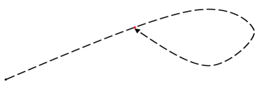
(a)

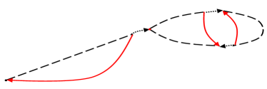
(b)

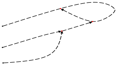
(c)

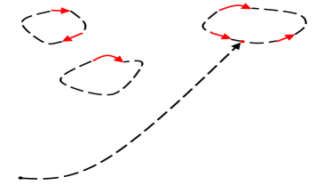
(d)

Figure 1: Collision-finding with multiple sources

Theorem 2.1.

There is an $O(k\log n)$ space deterministic algorithm Collide_k that, given $f:V\rightarrow V$ for a finite set $V$ and $K=\{v_{1},\ldots,v_{k}\}\subseteq V$, finds all pairs $\left(v,\left\{u\in f^{*}(K)\middle|f(u)=v\right\}\right)$ and runs in time $O(|f^{*}(K)|\log k\min\{k,\log n\})$.

Proof.

We first describe the algorithm Collide_k: In addition to the original graph and the collisions that it finds, this algorithm will maintain a redirection list $R\subset V$ of size $O(k)$ vertices that it will provisionally redirect to map to a different location. For each vertex in $R$ it will store the name of the new vertex to which it is directed. We maintain a separate list $L$ of all vertices from which an edge of $G$ has been redirected away and the original vertices that point to them.

Collide_k:
Set $R=\emptyset$.
For $j=1,\ldots,k$ do:

1. Execute Floyd’s algorithm starting with vertex $v_{j}$ on the graph $G$ using the redirected out-edges for nodes from the redirection list $R$ instead of $f$.

2. If the cycle found does not include $v_{j}$, there must be a collision.

   1. If this collision is in the graph $G$, report the collision $v$ as well as the colliding vertices $u$ and $u^{\prime}$, where $u^{\prime}$ is the predecessor of $v$ on the cycle and $u$ is the predecessor of $v$ on the path from $v_{j}$ to $v$.

   2. Add $u$ to the redirection list $R$ and redirect it to vertex $v_{j}$.

3. Traverse the cycle again to find its length and choose two vertices $w$ and $w^{\prime}$ on the cycle that are within 1 of half this length apart. Add $w$ and $w^{\prime}$ to the redirection list, redirecting $w$ to $f(w^{\prime})$ and $w^{\prime}$ to $f(w)$. This will split the cycle into two parts, each of roughly half its original length.

The redirections for a single iteration of the algorithm are shown in Figure 1(b). The general situation for later iterations in the algorithm is shown in Figure 1(d).

Observe that in each iteration of the loop there is at most one vertex $v$ where collisions can occur and at most 3 vertices are added to the redirection list. Moreover, after each iteration, the set of vertices reachable from vertices $v_{1},\ldots,v_{j}$ appear in a collection of disjoint cycles of the redirected graph. Each iteration of the loop traverses at most one cycle and every cycle is roughly halved each time it is traversed.

In order to store the redirection list $R$, we use a dynamic dictionary data structure of $O(k\log n)$ bits that supports insert and search in $O(\log k)$ time per access or insertion. We can achieve this using balanced binary search trees and we can improve the bound to $O{(\sqrt{\log k/\log\log k})}$ using exponential trees [6]. Before following an edge (i.e., evaluating $f$), the algorithm will first check list $R$ to see if it has been redirected. Hence each edge traversed costs $O(\log k)$ time (or $O{(\sqrt{\log k/\log\log k})}$ using exponential trees). Since time is measured relative to the size of the reachable set of vertices, the only other extra cost is that of re-traversing previously discovered edges. Since all vertices are maintained in cycles and each traversal of a cycle roughly halves its length, each edge found can be traversed at most $O(\min\{k,\log n\})$ times. ∎

As we have noted in the proof, with exponential trees the running time of the algorithm can be reduced to $O(|f^{*}(K)|\sqrt{\log k/\log\log k}\min\{k,\log n\})$, though the algorithm becomes significantly more complicated in this case.

2.2 A randomized $T^{2}\cdot S\in\tilde{O}(n^{3})$ element distinctness algorithm

We will use collision-finding for our element distinctness algorithm. In this case the vertex set $V$ will be the set of indices $[n]$, and the function $f$ will be given by $f_{x,h}(i)=h(x_{i})$ where $h$ is a (random) hash function that maps $[m]$ to $[n]$.

Observe that if we find $i\neq j$ such that $f_{x,h}(i)=f_{x,h}(j)$ then either

• $x_{i}=x_{j}$ and hence $\textsc{ED}(x)=0$, or

• we have found a collision in $h$: $x_{i}\neq x_{j}$ but $h(x_{i})=h(x_{j})$;

We call $x_{i}$ and $x_{j}$ “pseudo-duplicates” in this latter case.

Given a parameter $k$, on input $x$ our randomized algorithm will repeatedly choose a random hash function $h$ and a random set $K$ of roughly $k$ starting points and then call the Collide_k algorithm given in Theorem 2.1 on $K$ using the function $f=f_{x,h}$ and check the collisions found to determine whether or not there is a duplicate among the elements of $x$ indexed by $f_{x,h}^{*}(K)$. The space bound $S$ of this algorithm will be $O(k\log n)$.

The running time of Collide_k depends on $|f_{x,h}^{*}(K)|$, which in turn is governed by the random choices of $h$ and $K$ and may be large. Since $f_{x,h}^{*}(K)$ is also random, we also need to argue that if $ED(x)=0$, then there is a reasonable probability that a duplicate in $x$ will be found among the indices in $f_{x,h}^{*}(K)$. The following two lemmas analyze these issues.

Lemma 2.2.

Let $x\in[m]^{n}$. For $h:[m]\rightarrow[n]$ chosen uniformly at random and for $K\subseteq[n]$ selected by uniformly and independently choosing $2\leq k\leq n/32$ elements of $[n]$ with replacement, $\Pr[|f_{x,h}^{*}(K)|\leq 2\sqrt{kn}]\geq 8/9$.

Lemma 2.3.

Let $x\in[m]^{n}$ be such that $ED(x)=0$. Then for $h:[m]\rightarrow[n]$ chosen uniformly at random and for $K\subseteq[n]$ selected by uniformly and independently choosing $2\leq k\leq n/32$ elements of $[n]$ with replacement, $\Pr[|f_{x,h}^{*}(K)|\leq 2\sqrt{kn}\mbox{ and $\exists i\neq j\in f_{x,h}^{*}(K)$ such that $x_{i}=x_{j}$}]\geq k/(18n)$.

Before we prove these lemmas we show how, together with the properties of Collide_k, they yield the following theorem.

Theorem 2.4.

For any $\epsilon>0$, and any $S$ with $c\log n\leq S\leq n/32$ for some constant $c>0$, there is a randomized RAM algorithm with input randomness computing $ED_{n}$ with 1-sided error (false positives) at most $\epsilon$, that uses space $S$ and time $T\in O(\frac{n^{3/2}}{S^{1/2}}\log^{5/2}n\log(1/\epsilon))$. Further, when $S\in O(\log n)$, we have $T\in O(n^{3/2}\log(1/\epsilon))$.

Proof.

Choose $k\geq 2$ such that the space usage of Collide_k on $[n]$ is at most $S/2$. Therefore $k\in\Omega(S/\log n)$. The algorithm is as follows:

On input $x$, run $(18n/k)\log(1/\epsilon)$ independent runs of Collide_k on different $f_{x,h}$, each with independent random choices of hash functions $h$ and independent choices, $K$, of $k$ starting indices, and each with a run-time cut-off bounding the number of explored vertices of $f_{x,h}^{*}(K)$ at $t^{*}=2\sqrt{kn}$.
On each run, check if any of the collisions found is a duplicate in $x$, in which case output $ED(x)=0$ and halt. If none are found in any round then output $ED(x)=1$.

The algorithm will never incorrectly report a duplicate in a distinct $x$ and by Lemma 2.3, each run has a probability of at least $k/(18n)$ of finding a duplicate in an input $x$ such that $ED(x)=0$ so the probability of failing to find a duplicate in $(18n/k)\log(1/\epsilon)$ rounds is at most $\epsilon$.

Using Theorem 2.1 each run of our bounded version of Collide_k, requires runtime $O(\sqrt{kn}\log k\min\{k,\log n\})$ and hence the total runtime of the algorithm is $O(\sqrt{kn}\cdot n/k\cdot\log k\min\{k,\log n\}\log(1/\epsilon))$ which is $O(n^{3/2}\log(1/\epsilon))$ for $k$ constant and $O(n^{3/2}/k^{1/2}\cdot\log^{2}n\cdot\log(1/\epsilon))$ for general $k$. The claim follows using $k\in\Omega(S/\log n)$.

∎

To complete the proof of Theorem 2.4, we now prove the two technical lemmas on properties of $f_{x,h}^{*}(K)$ that the randomization in the hash functions. In particular, we first prove Lemma 2.2 showing that for any $x$, $f_{x,h}^{*}(K)$ is typically not larger than $2\sqrt{kn}$.

Proof of Lemma 2.2.

We can run an experiment that is equivalent to selecting $f_{x,h}^{*}(K)$ as follows:

Set $M=I=K=\emptyset$.
For	$count=1$ to $k$ do
	Choose an element $i\in[n]$ uniformly at random and add it to $K$.
	While	$i\notin I$ do
		Add $i$ to $I$
		If	$x_{i}\notin M$ then
			Add $x_{i}$ to $M$
			Choose an element $i\in[n]$ uniformly at random.
		else exit while loop and output (“duplicate found”)
	End While
End For
Output $I$.

Observe that, when each new element $i$ is chosen at random, the probability that a previous index is found (the while loop exits) is precisely $|I|/n$ and that $|I|$ increases by 1 per step, except for the $k$ steps when $i$ was already in $I$ or $x_{i}$ was in $M$. View each of these random choices of $i$ as a coin-flip with probability of heads being $|I|/n$.

The index set size $|I|$ at the $j$-th random choice is at least $j-k$ as we will have seen a duplicate in either $I$ or $M$ at most $k$ times. Hence the probability of exiting the while loop is at least $(j-k)/n$. Therefore the expected number of while loop exits that have occurred when the $t$-th random choice is made is at least $\sum_{j=1}^{t-k}j/n$. Consider for a moment our experiment but with the bound on the for loop removed. Then, solving for $t$ we get that the minimum number of random choices at which the expected number of while loop exits is at least $k/(1-\delta)$ is itself at least $\lceil(\sqrt{1+8kn/(1-\delta)}-1)/2+k\rceil\leq\sqrt{2kn/(1-\delta)}+k+1$. Let $\delta=3/4$ and observe that $n>32k$ implies that $\sqrt{8kn/3}+k+1\leq 2\sqrt{kn}$. Our experiment terminates when $\text{count}>k$ and so we can now bound the number of random choices and hence $|f_{k,n}^{*}(K)|$. By treating the event of exiting the while loop as independent coin flips with the lower bound probability of $(j-k)/n$ at random choice $j$ and applying the Chernoff inequality, we get that $\Pr[|f_{k,n}^{*}(K)|>2\sqrt{kn}]\leq e^{-9k/8}$ as required to prove the lemma. ∎

Finally we prove Lemma 2.3 showing that any duplicate in $x$ is also somewhat likely to be found in $f_{x,h}^{*}(K)$.

Proof of Lemma 2.3.

We show this first for an $x$ that has a single pair of duplicated values and then observe how this extends to the general case. Consider the sequence of indices selected in the experiment in the proof of Lemma 2.2 on input $x$. We define an associated Markov chain with a state $S(d,j,b)$ for $0\leq d<n$, for $0\leq j\leq k-1$, and for $b\in\{0,1\}$, where state $S(d,j,b)$ indicates that there have been $d$ distinct indices selected so far, $j$ pseudo-duplicates, and $b$ is the number of indices from the duplicated pair selected so far. In addition, the chain has two absorbing states, $F$, indicating that a duplicate has been found, and $N$, indicating that no duplicates have been found at termination.

Observe that the probability in state $S(d,j,b)$ that the next selection is a pseudo-duplicate is precisely $d/n$; hence it is also the probability of a transition from $S(d,j,b)$ to $S(d,j+1,b)$ if $j<k-1$, or to $N$ if $j=k-1$. From state $S(d,j,0)$ there is a $2/n$ chance of selecting one of the duplicated pair, so this is the probability of the transition from $S(d,j,0)$ to $S(d+1,j,1)$. Finally, from state $S(d,j,1)$, the probability that the other element of the duplicated pair is found is precisely $1/n$ and so this is the probability of a transition to $F$. The remaining transition from state from $S(d,j,b)$ leads to state $S(d+1,j,b)$ with probability $1-(d+2-b)/n$. See Figure 2.

Figure 2: Transitions from the Markov chain in the proof of Lemma 2.3

By the result of Lemma 2.2, with probability at least $8/9$, when started in state $S(0,0,0)$ this chain reaches state $F$ or $N$ in at most $t^{*}=2\sqrt{kn}$ steps. The quantity we wish to lower bound is the probability that the chain reaches state $F$ in its first $t^{*}$ steps. We derive our bound by comparing the probability that $F$ is reached in $t^{*}$ steps to the probability that either $F$ or $N$ is reached in $t^{*}$ steps.

Consider all special transitions, those that increase $j$ or $b$, or result in states $F$ or $N$. In any walk on the Markov chain that reaches $F$ or $N$, at most $k+1$ special transitions can be taken, and to reach $N$, at least $k$ special transitions must be taken.

Fix any sequence $0\leq d_{1}\leq\ldots\leq d_{k+1}<t^{*}$. We say that a walk on the Markov chain is consistent with this sequence iff the sequence of starting states of its special transitions is a prefix of some sequence of states $S(d_{1},*,*),\ldots,S(d_{k+1},*,*)$. We condition on the walk being one of these consistent walks.

Assume that $k\geq 2$. In order to reach state $F$, there must be one special transition that changes $b$ from 0 to 1 and another that leads to $F$. Consider the choices $(a,a^{\prime})\in\binom{[k]}{2}$ of where these can occur among the first $k$ special transitions. The conditional probability that a consistent special transition goes from $S(d_{a},j_{a},0)$ to $S(d_{a}+1,j_{a},1)$ is precisely $2/(d_{a}+2)\geq 1/t^{*}$ and the conditional probability that it goes from $S(d_{a^{\prime}},j_{a^{\prime}},1)$ to $F$ is precisely $1/(d_{a^{\prime}}+1)\geq 1/t^{*}$. In particular, the conditional probability that two special transitions of these types occur is lower bounded by the probability that $k$ Bernoulli trials with success probability $1/t^{*}$ yield at least two successes. This lower bound is at least

$$\binom{k}{2}1/(t^{*})^{2}(1-1/t^{*})^{k-2} \geq[1-(k-2)/t^{*}]\cdot\binom{k}{2}/(t^{*})^{2}$$

$$\geq[1-(k-2)/(2\sqrt{kn})]k(k-1)/(8kn)\geq k/(16n).$$

Since the different sequences correspond to disjoint sets of inputs, conditioned on the event that $F$ or $N$ is reached in at most $t^{*}$ steps, which occurs with probability at least $8/9$, the conditional probability that $F$ is reached is $\geq k/(16n)$. Therefore the total probability that $F$ is reached in at most $t^{*}$ steps is at least $k/(18n)$, as required.

In the general case, we observe that at each step prior to termination, the probability of finding a pseudo-duplicate, given that $j$ of them have previously been found, does not depend on $x$. On the other hand, additional duplicated inputs in $x$ only increase the chance of selecting a first index that is duplicated, and can only increase the chance that one of its matching indices will be selected in subsequent choices. Therefore, finding a duplicate is at least as likely for $x$ as it is in the above analysis. ∎

3 Sliding Windows

Let $D$ and $R$ be two finite sets and $f:D^{n}\rightarrow R$ be a function over strings of length $n$. We define the operation $\boxplus$ which takes $f$ and returns a function $f^{\boxplus t}:D^{n+t-1}\rightarrow R^{t}$, defined by $f^{\boxplus t}(x)=\left(f(x_{i}\ldots x_{i+n-1})\right)_{i=1}^{t}$. Because it produces a large number of outputs while less than doubling the input size, we concentrate on the case that $t=n$ and apply the $\boxplus$ operator to the statistical functions $F_{k}$, $F_{k}\bmod 2$, $ED$, and $O_{t}$, the $t^{th}$ order statistic. We will use the notation $F_{k}^{(j)}$ (resp. $f_{i}^{(j)}$) to denote the $k^{th}$ frequency moment (resp. the frequency of symbol $i$) of the string in the window of length $n$ starting at position $j$.

3.1 Element Distinctness over Sliding Windows

The main result of this section shows that our randomized branching program for $ED_{n}$ can even be extended to a $T\in\tilde{O}(n^{3/2}/S^{1/2})$ randomized branching program for its sliding windows version $ED_{n}^{\boxplus n}$. We do this in two steps. We first give a deterministic reduction which shows how the answer to an element distinctness problem allows one to reduce the input size of sliding-window algorithms for computing $ED_{n}^{\boxplus m}$.

Lemma 3.1.

Let $n>m>0$.

1. If $ED_{n-m+1}(x_{m},\ldots,x_{n})=0$ then $ED_{n}^{\boxplus m}(x_{1},\ldots,x_{n+m-1})=0^{m}$.

2. If $ED_{n-m+1}(x_{m},\ldots,x_{n})=1$ then define

   1. $i_{L}=\max\{j\in[m-1]\mid ED_{n-j+1}(x_{j},\ldots,x_{n})=0\}$ where $i_{L}=0$ if the set is empty and

   2. $i_{R}=\min\{j\in[m-1]\mid ED_{n-m+j}(x_{m},\ldots,x_{n+j})=0\}$ where $i_{R}=m$ if the set is empty.

   Then

   $$ED_{n}^{\boxplus m}(x_{1},\ldots,x_{n+m-1})=0^{i_{L}}1^{m-i_{L}}\ \land\ 1^{i_{R}}0^{m-i_{R}}\ \land\ ED_{m-1}^{\boxplus m}(x_{1},\ldots,x_{m-1},x_{n+1},\ldots,x_{n+m-1})$$

   where each $\land$ represents bit-wise conjunction.

Proof.

The elements $M=(x_{m},\ldots,x_{n})$ appear in all $m$ of the windows so if this sequence contains duplicated elements, so do all of the windows and hence the output for all windows is $0$. This implies part (a).

If $M$ does not contain any duplicates then any duplicate in a window must involve at least one element from $L=(x_{1},\ldots,x_{m-1})$ or from $R=(x_{n+1},\ldots,x_{n+m-1})$. If a window has value 0 because it contains an element of $L$ that also appears in $M$, it must also contain the rightmost such element of $L$ and hence any window that is distinct must begin to the right of this rightmost such element of $L$. Similarly, if a window has value 0 because it contains an element of $R$ that also appears in $M$, it must also contain the leftmost such element of $R$ and hence any window that is distinct must end to the left of this leftmost such element of $R$. The only remaining duplicates that can occur in a window can only involve elements of both $L$ and $R$. In order, the $m$ windows contain the following sequences of elements of $L\cup R$: $(x_{1},\ldots,x_{m-1})$, $(x_{2},\ldots,x_{m-1},x_{n+1})$, $\ldots$, $(x_{m-1},x_{n+1},\ldots,x_{n+m-2})$, $(x_{n+1},\ldots,x_{n+m-1})$. These are precisely the sequences for which $ED_{m-1}^{\boxplus m}(x_{1},\ldots,x_{m-1},x_{n+1},\ldots,x_{n+m-1})$ determines distinctness. Hence part (b) follows. ∎

We use the above reduction in input size to show that any efficient algorithm for element distinctness can be extended to solve element distinctness over sliding windows at a small additional cost.

Lemma 3.2.

If there is an algorithm $A$ that solve element distinctness, $ED$, using time at most $T(n)$ and space at most $S(n)$, where $T$ and $S$ are nondecreasing functions of $n$, then there is an algorithm $A^{*}$ that solves the sliding-window version of element distinctness, $ED_{n}^{\boxplus n}$, in time $T^{*}(n)$ that is $O(T(n)\log^{2}n)$ and space $S^{*}(n)$ that is $O(S(n)+\log^{2}n)$. Moreover, if $T(n)$ is $\Omega(n^{\beta})$ for $\beta>1$, then $T^{*}(n)$ is $O(T(n)\log n)$.

If $A$ is deterministic then so is $A^{*}$. If $A$ is randomized with error at most $\epsilon$ then $A^{*}$ is randomized with error $o(1/n)$. Moreover, if $A$ has the obvious 1-sided error (it only reports that inputs are not distinct if it is certain of the fact) then the same property holds for $A^{*}$.

Proof.

We first assume that $A$ is deterministic. Algorithm $A^{*}$ will compute the $n$ outputs of $ED_{n}^{\boxplus n}$ in $n/m$ groups of $m$ using the input size reduction method from Lemma 3.1. In particular, for each group $A^{*}$ will first call $A$ on the middle section of input size $n-m+1$ and output $0^{m}$ if $A$ returns 0. Otherwise, $A^{*}$ will do two binary searches involving at most $2\log m$ calls to $A$ on inputs of size at most $n$ to compute $i_{L}$ and $i_{R}$ as defined in part (b) of that lemma. Finally, in each group, $A^{*}$ will make one recursive call to $A^{*}$ on a problem of size $m$.

It is easy to see that this yields a recurrence of the form

$$T^{*}(n)=(n/m)[cT(n)\log m+T^{*}(m)].$$

In particular, if we choose $m=n/2$ then we obtain $T^{*}(n)\leq 2T^{*}(n/2)+2cT(n)\log n$. If $T(n)$ is $\Omega(n^{\beta})$ for $\beta>1$ this solves to $T^{*}(n)\in O(T(n)\log n)$. Otherwise, it is immediate from the definition of $T(n)$ that $T(n)$ must be $\Omega(n)$ and hence the recursion for $A^{*}$ has $O(\log n)$ levels and the total cost associated with each of the levels of the recursion is $O(T(n)\log n)$.

Observe that the space for all the calls to $A$ can be re-used in the recursion. Also note that the algorithm $A^{*}$ only needs to remember a constant number of pointers for each level of recursion for a total cost of $O(\log^{2}n)$ additional bits.

We now suppose that the algorithm $A$ is randomized with error at most $\epsilon$. For the recursion based on Lemma 3.1, we use algorithm $A$ and run it $C=O(\log n)$ times on input $(x_{m},\ldots,x_{n})$, taking the majority of the answers to reduce the error to $o(1/n^{2})$. In case that no duplicate is found in these calls, we then apply the noisy binary search method of Feige, Peleg, Raghavan, and Upfal [21] to determine $i_{L}$ and $i_{R}$ with error at most $o(1/n^{2})$ by using only $C=O(\log n)$ calls to $A$. (If the original problem size is $n$ we will use the same fixed number $C=O(\log n)$ of calls to $A$ even at deeper levels of the recursion so that each subproblem has error $o(1/n^{2})$.) There are only $O(n)$ subproblems so the final error is $o(1/n)$. The rest of the run-time analysis is the same as in the deterministic case.

If $A$ has only has false positives (if it claims that the input is not distinct then it is certain that there is a duplicate) then observe that $A^{*}$ will only have false positives. ∎

Combining Theorem 2.4 with Lemma 3.2 we obtain our algorithm for element distinctness over sliding windows.

Theorem 3.3.

For space $S\in[c\log n,n]$, $ED^{\boxplus n}$ can be solved in time $T\in O(n^{3/2}\log^{7/2}{n}/S^{1/2})$ with $1$-sided error probability $o(1/n)$. If the space $S\in O(\log{n})$ then the time is reduced to $T\in O{\left(n^{3/2}\log{n}\right)}$.

When the input alphabet is chosen uniformly at random from $[n]$ there exists a much simpler $0$-error sliding-window algorithm for $ED^{\boxplus n}$ that is efficient on average. The algorithm runs in $O(n)$ time on average using $O(\log{n})$ bits of space. By way of contrast, under the same distribution, we prove an average case time-space lower bound of $\overline{T}\in\Omega(n^{2}/\overline{S})$ for $(F_{0}\bmod 2)^{\boxplus n}$ in Section 3.2. The proof is in Appendix A.

Theorem 3.4.

For input randomly chosen uniformly from $[n]^{2n-1}$, $ED^{\boxplus n}$ can be solved in average time $\overline{T}\in O(n)$ and average space $\overline{S}\in O(\log{n})$.

3.2 Frequency Moments over Sliding Windows

We now show a $T\in\Omega(n^{2}/S)$ lower bound for randomized branching programs computing frequency moments over sliding windows. This contrasts with our significantly smaller $T\in\tilde{O}(n^{3/2}/S^{1/2})$ upper bound from the previous section for computing element distinctness over sliding windows in this same model, hence separating the complexity of $ED$ and $F_{k}$ for $k\neq 1$ over sliding windows. Our lower bound also applies to $F_{0}\bmod 2$.

3.2.1 A general sequential lower bound for $F_{k}^{\boxplus n}$ and $(F_{0}\bmod 2)^{\boxplus n}$

We derive a time-space tradeoff lower bound for randomized branching programs computing $F_{k}^{\boxplus n}$ for $k=0$ and $k\geq 2$. Further, we show that the lower bound also holds for computing $(F_{0}\bmod 2)^{\boxplus n}$. (Note that the parity of $F_{k}$ for $k\geq 1$ is exactly equal to the parity of $n$; thus the outputs of $(F_{k}\bmod 2)^{\boxplus n}$ are all equal to $n\bmod 2$.)

Theorem 3.5.

Let $k=0$ or $k\geq 2$. There is a constant $\delta>0$ such that any $[n]$-way branching program of time $T$ and space $S$ that computes $F_{k}^{\boxplus n}$ with error at most $\eta$, $0<\eta<1-2^{-\delta S}$, for input randomly chosen uniformly from $[n]^{2n-1}$ must have $T\cdot S\in\Omega(n^{2})$. The same lower bound holds for $(F_{0}\bmod 2)^{\boxplus n}$.

Corollary 3.6.

Let $k=0$ or $k\geq 2$.

• The average time $\overline{T}$ and average space $\overline{S}$ needed to compute $(F_{k})^{\boxplus n}(x)$ for $x$ randomly chosen uniformly from $[n]^{2n-1}$ satisfy $\overline{T}\cdot\overline{S}\in\Omega(n^{2})$.

• For $0<\eta<1-2^{-\delta S}$, any $\eta$-error randomized RAM or word-RAM algorithm computing $(F_{k})^{\boxplus n}$ using time $T$ and space $S$ satisfies $T\cdot S\in\Omega(n^{2})$.

Proof of Theorem 3.5.

We derive the lower bound for $F_{0}^{\boxplus n}$ first. Afterwards we show the modifications needed for $k\geq 2$ and for computing $(F_{0}\bmod 2)^{\boxplus n}$. For convenience, on input $x\in[n]^{2n-1}$, we write $y_{i}$ for the output $F_{k}(x_{i},\ldots,x_{i+n-1})$.

We use the general approach of Borodin and Cook [12] together with the observation of [3] of how it applies to average case complexity and randomized branching programs. In particular, we divide the branching program $B$ of length $T$ into layers of height $q$ each. Each layer is now a collection of small branching programs $B^{\prime}$, each of whose start node is a node at the top level of the layer. Since the branching program must produce $n$ outputs for each input $x$, for every input $x$ there exists a small branching program $B^{\prime}$ of height $q$ in some layer that produces at least $nq/T>S$ outputs. There are at most $2^{S}$ nodes in $B$ and hence there are at most $2^{S}$ such small branching programs among all the layers of $B$. One would normally prove that the fraction of $x\in[n]^{2n-1}$ for which any one such small program correctly produces the desired number of outputs is much smaller than $2^{-S}$ and hence derive the desired lower bound. Usually this is done by arguing that the fraction of inputs consistent with any path in such a small branching program for which a fixed set of outputs is correct is much smaller than $2^{-S}$.

This basic outline is more complicated in our argument. One issue is that if a path in a small program $B^{\prime}$ finds that certain values are equal, then the answers to nearby windows may be strongly correlated with each other; for example, if $x_{i}=x_{i+n}$ then $y_{i}=y_{i+1}$. Such correlations risk making the likelihood too high that the correct outputs are produced on a path. Therefore, instead of considering the total number of outputs produced, we reason about the number of outputs from positions that are not duplicated in the input and argue that with high probability there will be a linear number of such positions.

A second issue is that inputs for which the value of $F_{0}$ in a window happens to be extreme, say $n$ - all distinct - or 1 - all identical, allow an almost-certain prediction of the value of $F_{0}$ for the next window. We will use the fact that under the uniform distribution, cases like these almost surely do not happen; indeed the numbers of distinct elements in every window almost surely fall in a range close to their mean and in this case the value in the next window will be predictable with probability bounded below 1 given the value in the previous ones. In this case we use the chain rule to compute the overall probability of correctness of the outputs.

We start by analyzing the likelihood that an output of $F_{0}$ is extreme.

Lemma 3.7.

Let $a$ be chosen uniformly at random from $[n]^{n}$. Then the probability that $F_{0}(a)$ is between $0.5n$ and $0.85n$ is at least $1-2e^{-n/50}$.

Proof.

For $a=a_{1}\ldots a_{n}$ uniformly chosen from $[n]^{n}$,

$$\mathbb{E}[F_{0}(a)]=\sum_{\ell\in[n]}\Pr_{a}[\exists i\in[n]\mbox{ such that }a_{i}=\ell]=n[1-(1-1/n)^{n}].$$

Hence $0.632n<(1-1/e)n<\mathbb{E}[F_{0}(a)]\leq 0.75n$. Define a Doob martingale $D_{t}$, $t=0,1,\ldots,n$ with respect to the sequence $a_{1}\ldots a_{n}$ by $D_{t}=\mathbb{E}[F_{0}(a)\mid a_{1}\ldots a_{t}]$. Therefore $D_{0}=\mathbb{E}[F_{0}(a)]$ and $D_{n}=F_{0}(a)$. Applying the Azuma-Hoeffding inequality, we have

$$\Pr_{a}[F_{0}(a)\notin[0.5n,0.85n]]\leq\Pr_{a}[|F_{0}(a)-\mathbb{E}[F_{0}(a)|\geq 0.1n]\leq 2e^{-2\frac{(0.1n)^{2}}{n}}=2e^{-n/50},$$

which proves the claim. ∎

We say that $x_{j}$ is unique in $x$ iff $x_{j}\notin\{x_{1},\ldots,x_{j-1},x_{j+1},\ldots,x_{2n-1}\}$.

Lemma 3.8.

Let $x$ be chosen uniformly at random from $[n]^{2n-1}$ with $n\geq 2$. With probability at least $1-4ne^{-n/50}$,

1. all outputs of $F_{0}^{\boxplus n}(x)$ are between $0.5n$ and $0.85n$, and

2. the number of positions $j<n$ such that $x_{j}$ is unique in $x$ is at least $n/24$.

Proof.

We know from Lemma 3.7 and the union bound that part (a) is false with probability at most $2ne^{-n/50}$. For any $j<n$, let $U_{j}$ be the indicator variable of the event that $j$ is unique in $x$ and $U=\sum_{j<n}U_{j}$. Now $\mathbb{E}(U_{j})=(1-1/n)^{2n-2}$ so $\mathbb{E}(U)=(n-1)(1-1/n)^{2n-2}\geq n/8$ for $n\geq 2$. Observe also that this is a kind of typical “balls in bins” problem and so, as discussed in [20], it has the property that the random variables $U_{j}$ are negatively associated; for example, for disjoint $A,A^{\prime}\subset[n-1]$, the larger $\sum_{j\in A}U_{j}$ is, the smaller $\sum_{j\in A^{\prime}}U_{j}$ is likely to be. Hence, it follows [20] that $U$ is more closely concentrated around its mean than if the $U_{j}$ were fully independent. It also therefore follows that we can apply a Chernoff bound directly to our problem, giving $\Pr[U\leq n/24]\leq\Pr[U\leq\mathbb{E}(U)/3]\leq e^{-2\mathbb{E}(U)/9}\leq e^{-n/36}$. We obtain the desired bound for parts (a) and (b) together by another application of the union bound. ∎

Correctness of a small branching program for computing outputs in $\pi$-unique positions

Definition 3.1.

Let $B^{\prime}$ be an $[n]$-way branching program and let $\pi$ be a source-sink path in $B^{\prime}$ with queries $Q_{\pi}$ and answers $A_{\pi}:Q_{\pi}\rightarrow[n]$. An index $\ell<n$ is said to be $\pi$-unique iff either (a) $\ell\notin Q_{\pi}$, or (b) $A_{\pi}(\ell)\notin A_{\pi}(Q_{\pi}-\{\ell\})$.

In order to measure the correctness of a small branching program, we restrict our attention to outputs that are produced at positions that are $\pi$-unique and upper-bound the probability that a small branching program correctly computes outputs of $F_{0}^{\boxplus n}$ at many $\pi$-unique positions in the input.

Let $\mathcal{E}$ be the event that all outputs of $F_{0}^{\boxplus n}(x)$ are between $0.5n$ and $0.85n$.

Lemma 3.9.

Let $r>0$ be a positive integer, let $\epsilon\leq 1/10$, and let $B^{\prime}$ be an $[n]$-way branching program of height $q=\epsilon n$. Let $\pi$ be a path in $B^{\prime}$ on which outputs from at least $r$ $\pi$-unique positions are produced. For random $x$ uniformly chosen from $[n]^{2n-1}$,

$$\Pr[\mbox{these $r$ outputs are correct for $F_{0}^{\boxplus n}(x)$},\mathcal{E}\mid\pi_{B^{\prime}}(x)=\pi]\leq(17/18)^{r}.$$

Proof.

Roughly, we will show that when $\mathcal{E}$ holds (outputs for all windows are not extreme) then, conditioned on following any path $\pi$ in $B^{\prime}$, each output produced for a $\pi$-unique position will have only a constant probability of success conditioned on any outcome for the previous outputs. Because of the way outputs are indexed, it will be convenient to consider these outputs in right-to-left order.

Let $\pi$ be a path in $B^{\prime}$, $Q_{\pi}$ be the set of queries along $\pi$, $A_{\pi}:Q_{\pi}\rightarrow[n]$ be the answers along $\pi$, and $Z_{\pi}:[n]\rightarrow[n]$ be the partial function denoting the outputs produced along $\pi$. Note that $\pi_{B^{\prime}}(x)=\pi$ if and only if $x_{i}=A_{\pi}(i)$ for all $i\in Q_{\pi}$.

Let $1\leq i_{1}<i_{2}<\ldots<i_{r}<n$ be the first $r$ of the $\pi$-unique positions on which $\pi$ produces output values; i.e., $\{i_{1},\ldots,i_{r}\}\subseteq\mathrm{dom}(Z_{\pi})$. Define $z_{i_{1}}=Z_{\pi}(i_{1}),\ldots,z_{i_{r}}=Z_{\pi}(i_{r})$.

We will decompose the probability over the input $x$ that $\mathcal{E}$ and all of $y_{i_{1}}=z_{i_{1}},\ldots,y_{i_{r}}=z_{i_{r}}$ hold via the chain rule. In order to do so, for $\ell\in[r]$, we define event $\mathcal{E}_{\ell}$ to be $0.5n\leq F_{0}^{(i)}(x)\leq 0.85n$ for all $i>i_{\ell}$. We also write $\mathcal{E}_{0}\mathrel{\overset{\makebox[0.0pt]{\mbox{\tiny def}}}{=}}\mathcal{E}$. Then

$$\Pr[y_{i_{1}}=z_{i_{1}},\ldots,y_{i_{r}}=z_{i_{r}},\ \mathcal{E}\mid\pi_{B^{\prime}}(x)=\pi]$$

$$=\Pr[\mathcal{E}_{r}\mid\pi_{B^{\prime}}(x)=\pi]\cdot\prod_{\ell=1}^{r}\Pr[y_{i_{\ell}}=z_{i_{\ell}},\ \mathcal{E}_{\ell-1}\mid y_{i_{\ell+1}}=z_{i_{\ell+1}},\ \ldots,\ y_{i_{r}}=z_{i_{r}},\ \mathcal{E}_{\ell},\ \pi_{B^{\prime}}(x)=\pi]$$

(1) $$\leq\prod_{\ell=1}^{r}\Pr[y_{i_{\ell}}=z_{i_{\ell}}\mid y_{i_{\ell+1}}=z_{i_{\ell+1}},\ \ldots,\ y_{i_{r}}=z_{i_{r}},\ \mathcal{E}_{\ell},\ \pi_{B^{\prime}}(x)=\pi].$$

We now upper bound each term in the product in (1). Depending on how much larger $i_{\ell+1}$ is than $i_{\ell}$, the conditioning on the value of $y_{i_{\ell+1}}$ may imply a lot of information about the value of $y_{i_{\ell}}$, but we will show that even if we reveal more about the input, the value of $y_{i_{\ell}}$ will still have a constant amount of uncertainty.

For $i\in[n]$, let $W_{i}$ denote the vector of input elements $(x_{i},\ldots,x_{i+n-1})$, and note that $y_{i}=F_{0}(W_{i})$; we call $W_{i}$ the $i^{\mathrm{th}}$ window of $x$. The values $y_{i}$ for different windows may be closely related. In particular, adjacent windows $W_{i}$ and $W_{i+1}$ have numbers of distinct elements that can differ by at most 1 and this depends on whether the extreme end-points of the two windows, $x_{i}$ and $x_{i+n}$, appear among their common elements $C_{i}=\{x_{i+1},\ldots,x_{i+n-1}\}$. More precisely,

(2) $$y_{i}-y_{i+1}=\textbf{1}_{\{x_{i}\not\in C_{i}\}}-\textbf{1}_{\{x_{i+n}\not\in C_{i}\}}.$$

In light of (2), the basic idea of our argument is that, because $i_{\ell}$ is $\pi$-unique and because of the conditioning on $\mathcal{E}_{\ell}$, there will be enough uncertainty about whether or not $x_{i_{\ell}}\in C_{i_{\ell}}$ to show that the value of $y_{i_{\ell}}$ is uncertain even if we reveal

1. the value of the indicator $\textbf{1}_{\{x_{i_{\ell}+n}\not\in C_{i_{\ell}}\}}$, and

2. the value of the output $y_{i_{\ell}+1}$.

We now make this idea precise in bounding each term in the product in (1), using $\mathcal{G}_{\ell+1}$ to denote the event $\{y_{i_{\ell+1}}=z_{i_{\ell+1}},\ \ldots,\ y_{i_{r}}=z_{i_{r}}\}$.

$$\Pr [y_{i_{\ell}}=z_{i_{\ell}}\mid\mathcal{G}_{\ell+1},\ \mathcal{E}_{\ell},\ \pi_{B^{\prime}}(x)=\pi]$$

$$= \sum_{m=1}^{n}\sum_{b\in\{0,1\}}\Pr[y_{i_{\ell}}=z_{i_{\ell}}\mid y_{i_{\ell}+1}=m,\textbf{1}_{\{x_{i_{\ell}+n}\not\in C_{i_{\ell}}\}}=b,\mathcal{G}_{\ell+1},\mathcal{E}_{\ell},\pi_{B^{\prime}}(x)=\pi]$$

$$\qquad\times\Pr[y_{i_{\ell}+1}=m,\textbf{1}_{\{x_{i_{\ell}+n}\not\in C_{i_{\ell}}\}}=b\mid\mathcal{G}_{\ell+1},\mathcal{E}_{\ell},\pi_{B^{\prime}}(x)=\pi]$$

$$\leq \max_{\begin{subarray}{c}m\in[0.5n,0.85n]\\ b\in\{0,1\}\end{subarray}}\Pr[y_{i_{\ell}}=z_{i_{\ell}}\mid y_{i_{\ell}+1}=m,\textbf{1}_{\{x_{i_{\ell}+n}\not\in C_{i_{\ell}}\}}=b,\mathcal{G}_{\ell+1},\mathcal{E}_{\ell},\pi_{B^{\prime}}(x)=\pi]$$

$$= \max_{\begin{subarray}{c}m\in[0.5n,0.85n]\\ b\in\{0,1\}\end{subarray}}\Pr[\textbf{1}_{\{x_{i_{\ell}}\not\in C_{i_{\ell}}\}}=z_{i_{\ell}}-m+b\mid$$

(3) $$\qquad\qquad\qquad\qquad y_{i_{\ell}+1}=m,\textbf{1}_{\{x_{i_{\ell}+n}\not\in C_{i_{\ell}}\}}=b,\mathcal{G}_{\ell+1},\mathcal{E}_{\ell},\pi_{B^{\prime}}(x)=\pi]$$

where the inequality follows because the conditioning on $\mathcal{E}_{\ell}$ implies that $y_{i_{\ell}+1}$ is between $0.5n$ and $0.85n$ and the last equality follows because of the conditioning together with (2) applied with $i=i_{\ell}$. Obviously, unless $z_{i_{\ell}}-m+b\in\{0,1\}$ the probability of the corresponding in the maximum in (3) will be 0. We will derive our bound by showing that given all the conditioning in (3), the probability of the event $\{x_{i_{\ell}}\not\in C_{i_{\ell}}\}$ is between $2/5$ and $17/18$ and hence each term in the product in (1) is at most $17/18$.

Membership of $x_{i_{\ell}}$ in $C_{i_{\ell}}$:

First note that the conditions $y_{i_{\ell}+1}=m$ and $\textbf{1}_{\{x_{i_{\ell}+n}\not\in C_{i_{\ell}}\}}=b$ together imply that $C_{i_{\ell}}$ contains precisely $m-b$ distinct values. We now use the fact that $i_{\ell}$ is $\pi$-unique and, hence, either $i_{\ell}\notin Q_{\pi}$ or $A_{\pi}(i_{\ell})\notin A_{\pi}(Q_{\pi}-\{i_{\ell}\})$.

First consider the case that $i_{\ell}\notin Q_{\pi}$. By definition, the events $y_{i_{\ell}+1}=m$, $\textbf{1}_{\{x_{i_{\ell}+n}\not\in C_{i_{\ell}}\}}=b$, $\mathcal{E}_{\ell}$, and $\mathcal{G}_{\ell+1}$ only depend on $x_{i}$ for $i>i_{\ell}$ and the conditioning on $\pi_{B^{\prime}}(x)=\pi$ is only a property of $x_{i}$ for $i\in Q_{\pi}$. Therefore, under all the conditioning in (3), $x_{i_{\ell}}$ is still a uniformly random value in $[n]$. Therefore the probability that $x_{i_{\ell}}\in C_{i_{\ell}}$ is precisely $(m-b)/n$ in this case.

Now assume that $i_{\ell}\in Q_{\pi}$. In this case, the conditioning on $\pi_{B^{\prime}}(x)=\pi$ implies that $x_{i_{\ell}}=A_{\pi}(i_{\ell})$ is fixed and not in $A_{\pi}(Q_{\pi}-\{i_{\ell}\})$. Again, from the conditioning we know that $C_{i_{\ell}}$ contains precisely $m-b$ distinct values. Some of the elements that occur in $C_{i_{\ell}}$ may be inferred from the conditioning – for example, their values may have been queried along $\pi$ – but we will show that there is significant uncertainty about whether any of them equals $A_{\pi}(i_{\ell})$. In this case we will show that the uncertainty persists even if we reveal (condition on) the locations of all occurrences of the elements $A_{\pi}(Q_{\pi}-\{i_{\ell}\})$ among the $x_{i}$ for $i>i_{\ell}$.

Other than the information revealed about the occurrences of the elements $A_{\pi}(Q_{\pi}-\{i_{\ell}\})$ among the $x_{i}$ for $i>i_{\ell}$, the conditioning on the events $y_{i_{\ell}+1}=m$, $\textbf{1}_{\{x_{i_{\ell}+n}\not\in C_{i_{\ell}}\}}=b$, $\mathcal{E}_{\ell}$, and $\mathcal{G}_{\ell+1}$, only biases the numbers of distinct elements and patterns of equality among inputs $x_{i}$ for $i>i_{\ell}$. Further the conditioning on $\pi_{B^{\prime}(x)}=\pi$ does not reveal anything more about the inputs in $C_{i_{\ell}}$ than is given by the occurrences of $A_{\pi}(Q_{\pi}-\{i_{\ell}\})$. Let $\mathcal{A}$ be the event that all the conditioning is true.

Let $q^{\prime}=|A_{\pi}(Q_{\pi}-\{i_{\ell}\})|\leq q-1$ and let $q^{\prime\prime}\leq q^{\prime}$ be the number of distinct elements of $A_{\pi}(Q_{\pi}-\{i_{\ell}\})$ that appear in $C_{i_{\ell}}$. Therefore, since the input is uniformly chosen, subject to the conditioning, there are $m-b-q^{\prime\prime}$ distinct elements of $C_{i_{\ell}}$ not among $A_{\pi}(Q_{\pi}-\{i_{\ell}\})$, and these distinct elements are uniformly chosen from among the elements $[n]-A_{\pi}(Q_{\pi}-\{i_{\ell}\})$. Therefore, the probability that any of these $m-b-q^{\prime\prime}$ elements is equal to $x_{i_{\ell}}=A_{\pi}(i_{\ell})$ is precisely $(m-b-q^{\prime\prime})/(n-q^{\prime})$ in this case.

It remains to analyze the extreme cases of the probabilities $(m-b)/n$ and $(m-b-q^{\prime\prime})/(n-q^{\prime})$ from the discussion above. Since $q=\epsilon n$, $q^{\prime\prime}\leq q^{\prime}\leq q-1$, and $b\in\{0,1\}$, we have the probability $\Pr[x_{i_{\ell}}\in C_{i_{\ell}}\mid\mathcal{A}]\leq\frac{m}{n-q+1}\leq\frac{0.85n}{n-\epsilon n}\leq\frac{0.85n}{n(1-\epsilon)}\leq 0.85/(1-\epsilon)\leq 17/18$ since $\epsilon\leq 1/10$. Similarly, $\Pr[x_{i_{\ell}}\notin C_{i_{\ell}}\mid\mathcal{A}]<1-\frac{m-q}{n}\leq 1-\frac{0.5n-\epsilon n}{n}\leq 0.5+\epsilon\leq 3/5$ since $\epsilon\leq 1/10$. Plugging in the larger of these upper bounds in (1), we get:

$$\Pr[z_{i_{1}},\ldots,z_{i_{r}}\mbox{ are correct for }F_{0}^{\boxplus n}(x),\ \mathcal{E}\mid\pi_{B^{\prime}}(x)=\pi]\leq(17/18)^{r},$$

which proves the lemma. ∎

Putting the Pieces Together

We now combine the above lemmas. Suppose that $TS\leq n^{2}/4800$ and let $q=n/10$. We can assume without loss of generality that $S\geq\log_{2}n$ since we need $T\geq n$ to determine even a single answer.

Consider the fraction of inputs in $[n]^{2n-1}$ on which $B$ correctly computes $F_{0}^{\boxplus n}$. By Lemma 3.8, for input $x$ chosen uniformly from $[n]^{2n-1}$, the probability that $\mathcal{E}$ holds and there are at least $n/24$ positions $j<n$ such that $x_{j}$ is unique in $x$ is at least $1-4ne^{-n/50}$. Therefore, in order to be correct on any such $x$, $B$ must correctly produce outputs from at least $n/24$ outputs at positions $j<n$ such that $x_{j}$ is unique in $x$.

For every such input $x$, by our earlier outline, one of the $2^{S}$ $[n]$-way branching programs $B^{\prime}$ of height $q$ contained in $B$ produces correct output values for $F_{0}^{\boxplus n}(x)$ in at least $r=(n/24)q/T\geq 20S$ positions $j<n$ such that $x_{j}$ is unique in $x$.

We now note that for any $B^{\prime}$, if $\pi=\pi_{B^{\prime}}(x)$ then the fact that $x_{j}$ for $j<n$ is unique in $x$ implies that $j$ must be $\pi$-unique. Therefore, for all but a $4ne^{-n/50}$ fraction of inputs $x$ on which $B$ is correct, $\mathcal{E}$ holds for $x$ and there is one of the $\leq 2^{S}$ branching programs $B^{\prime}$ in $B$ of height $q$ such that the path $\pi=\pi_{B^{\prime}}(x)$ produces at least $20S$ outputs at $\pi$-unique positions that are correct for $x$.

Consider a single such program $B^{\prime}$. By Lemma 3.9 for any path $\pi$ in $B^{\prime}$, the fraction of inputs $x$ such that $\pi_{B^{\prime}}(x)=\pi$ for which $20S$ of these outputs are correct for $x$ and produced at $\pi$-unique positions, and $\mathcal{E}$ holds for $x$ is at most $(17/18)^{20S}<3^{-S}$. By Proposition 3.8, this same bound applies to the fraction of all inputs $x$ with $\pi_{B^{\prime}}(x)=\pi$ for which $20S$ of these outputs are correct from $x$ and produced at $\pi$-unique positions, and $\mathcal{E}$ holds for $x$ is at most $(17/18)^{20S}<3^{-S}$.

Since the inputs following different paths in $B^{\prime}$ are disjoint, the fraction of all inputs $x$ for which $\mathcal{E}$ holds and which follow some path in $B^{\prime}$ that yields at least $20S$ correct answers from distinct runs of $x$ is less than $3^{-S}$. Since there are at most $2^{S}$ such height $q$ branching programs, one of which must produce $20S$ correct outputs from distinct runs of $x$ for every remaining input, in total only a $2^{S}3^{-S}=(2/3)^{S}$ fraction of all inputs have these outputs correctly produced.

In particular this implies that $B$ is correct on at most a $4ne^{-n/50}+(2/3)^{S}$ fraction of inputs. For $n$ sufficiently large this is smaller than $1-\eta$ for any $\eta<1-2^{-\delta S}$ for some $\delta>0$, which contradicts our original assumption. This completes the proof of Theorem 3.5. ∎

Lower bound for $(F_{0}\bmod 2)^{\boxplus n}$

We describe how to modify the proof of Theorem 3.5 for computing $F_{0}^{\boxplus n}$ to derive the same lower bound for computing $(F_{0}\bmod 2)^{\boxplus n}$. The only difference is in the proof of Lemma 3.9. In this case, each output $y_{i}$ is $F_{0}(W_{i})\bmod 2$ rather than $F_{0}(W_{i})$ and (2) is replaced by

(4) $$y_{i}=(y_{i+1}+\textbf{1}_{\{x_{i}\not\in C_{i}\}}-\textbf{1}_{\{x_{i+n}\not\in C_{i}\}})\bmod 2.$$

The extra information revealed (conditioned on) will be the same as in the case for $F_{0}^{\boxplus n}$ but, because the meaning of $y_{i}$ has changed, the notation $y_{i_{\ell}+1}=m$ is replaced by $F_{0}(W_{i_{\ell}+1})=m$, $y_{i_{\ell}+1}$ is then $m\bmod 2$, and the upper bound in (3) is replaced by

$$\max_{\begin{subarray}{c}m\in[0.5n,0.85n]\\ b\in\{0,1\}\end{subarray}}\Pr[\textbf{1}_{\{x_{i_{\ell}}\not\in C_{i_{\ell}}\}}= (z_{i_{\ell}}-m+b)\bmod 2\mid$$

$$F_{0}(W_{i_{\ell}+1})=m,\textbf{1}_{\{x_{i_{\ell}+n}\not\in C_{i_{\ell}}\}}=b,\mathcal{G}_{\ell+1},\mathcal{E}_{\ell},\pi_{B^{\prime}}(x)=\pi]$$

The uncertain event is exactly the same as before, namely whether or not $x_{i_{\ell}}\in C_{i_{\ell}}$ and the conditioning is essentially exactly the same, yielding an upper bound of $17/18$. Therefore the analogue of Lemma 3.9 also holds for $(F_{0}\bmod 2)^{\boxplus n}$ and hence the time-space tradeoff of $T\cdot S\in\Omega(n^{2})$ follows as before.

Lower Bound for $F_{k}^{\boxplus n}$, $k\geq 2$

We describe how to modify the proof of Theorem 3.5 for computing $F_{0}^{\boxplus n}$ to derive the same lower bound for computing $F_{k}^{\boxplus n}$ for $k\geq 2$. Again, the only difference is in the proof of Lemma 3.9. The main change from the case of $F_{0}^{\boxplus n}$ is that we need to replace (2) relating the values of consecutive outputs. For $k\geq 2$, recalling that $f^{(i)}_{j}$ is the frequency of symbol $j$ in window $W_{i}$, we now have

(5) $$y_{i}-y_{i+1}=\left[\left(f^{(i)}_{x_{i}}\right)^{k}-\left(f^{(i)}_{x_{i}}-1\right)^{k}\right]-\left[\left(f^{(i+1)}_{x_{i+n}}\right)^{k}-\left(f^{(i+1)}_{x_{i+n}}-1\right)^{k}\right].$$

We follow the same outline as in the case $k=0$ in order to bound the probability that $y_{i_{\ell}}=z_{i_{\ell}}$ but we reveal the following information, which is somewhat more than in the $k=0$ case:

1. $y_{i_{\ell}+1}$, the value of the output immediately after $y_{i_{\ell}}$,

2. $F_{0}(W_{i_{\ell}+1})$, the number of distinct elements in $W_{i_{\ell}+1}$, and

3. $f^{(i_{\ell}+1)}_{x_{i_{\ell}+n}}$, the frequency of $x_{i_{\ell}+n}$ in $W_{i_{\ell}+1}$.

For $M\in\mathbb{N}$, $m\in[n]$ and $1\leq f\leq m$, define $\mathcal{C}_{M,m,f}$ be the event that $y_{i_{\ell}+1}=M$, $F_{0}(W_{i_{\ell}+1})=m$, and $f^{(i_{\ell}+1)}_{x_{i_{\ell}+n}}=f$. Note that $\mathcal{C}_{M,m,f}$ only depends on the values in $W_{i_{\ell}+1}$, as was the case for the information revealed in the case $k=0$. As before we can then upper bound the $\ell^{\mathrm{th}}$ term in the product given in (1) by

(6) $$\max_{\begin{subarray}{c}m\in[0.5n,0.85n]\\ M\in\mathbb{N},f\in[m]\end{subarray}}\Pr[y_{i_{\ell}}=z_{i_{\ell}}\mid\mathcal{C}_{M,m,f},\mathcal{G}_{\ell+1},\mathcal{E}_{\ell},\pi_{B^{\prime}}(x)=\pi]$$

Now, by (5), given event $\mathcal{C}_{M,m,f}$, we have $y_{i_{\ell}}=z_{i_{\ell}}$ if and only if $z_{i_{\ell}}-M=\left[\left(f^{(i_{\ell})}_{x_{i_{\ell}}}\right)^{k}-\left(f^{(i_{\ell})}_{x_{i_{\ell}}}-1\right)^{k}\right]-\left[f^{k}-(f-1)^{k}\right]$, which we can express as as a constraint on its only free parameter $f^{(i)}_{x_{i}}$,

$$\left(f^{(i_{\ell})}_{x_{i_{\ell}}}\right)^{k}-\left(f^{(i_{\ell})}_{x_{i_{\ell}}}-1\right)^{k}=z_{i_{\ell}}-M-f^{k}+(f-1)^{k}.$$

Observe that this constraint can be satisfied for at most one positive integer value of $f^{(i_{\ell})}_{x_{i_{\ell}}}$ and that, by definition, $f^{(i_{\ell})}_{x_{i_{\ell}}}\geq 1$. Note that $f^{(i_{\ell})}_{x_{i_{\ell}}}=1$ if and only if $x_{i_{\ell}}\notin C_{i_{\ell}}$, where $C_{i_{\ell}}$ is defined as in the case $k=0$. The probability that $f^{(i_{\ell})}_{x_{i_{\ell}}}$ takes on a particular value is at most the larger of the probability that $f^{(i_{\ell})}_{x_{i_{\ell}}}=1$ or that $f^{(i_{\ell})}_{x_{i_{\ell}}}>1$ and hence (6) is at most

$$\max_{\begin{subarray}{c}m\in[0.5n,0.85n]\\ M\in\mathbb{N},f\in[m],c\in\{0,1\}\end{subarray}}\Pr[\textbf{1}_{\{x_{i_{\ell}}\not\in C_{i_{\ell}}\}}=c\mid\mathcal{C}_{M,m,f},\mathcal{G}_{\ell+1},\mathcal{E}_{\ell},\pi_{B^{\prime}}(x)=\pi]$$

We now can apply similar reasoning to the $k=0$ case to argue that this is at most $17/18$: The only difference is that $\mathcal{C}_{M,m,f}$ replaces the conditions $y_{i_{\ell}+1}=F_{0}(W_{i_{\ell}+1})=m$ and $\textbf{1}_{\{x_{i_{\ell}+n}\not\in C_{i_{\ell}}\}}=b$. It is not hard to see that the same reasoning still applies with the new condition. The rest of the proof follows as before.

3.2.2 A time-space efficient algorithm for $F_{k}^{\boxplus n}$

We now show that our time-space tradeoff lower bound for $F_{k}^{\boxplus n}$ is nearly optimal even for restricted RAM models.

Theorem 3.10.

There is a comparison-based deterministic RAM algorithm for computing $F^{\boxplus n}_{k}$ for any fixed integer $k\geq 0$ with time-space tradeoff $T\cdot S\in O(n^{2}\log^{2}{n})$ for all space bounds $S$ with $\log n\leq S\leq n$.

Proof.

We denote the $i$-th output by $y_{i}=F_{k}(x_{i},\ldots,x_{i+n-1})$. We first compute $y_{1}$ using the comparison-based $O(n^{2}/S)$ time sorting algorithm of Pagter and Rauhe [30]. This algorithm produces the list of outputs in order by building a space $S$ data structure $D$ over the $n$ inputs and then repeatedly removing and returning the index of the smallest element from that structure using a POP operation. We perform POP operations on $D$ and keep track of the last index popped. We also will maintain the index $i$ of the previous symbol seen as well as a counter that tells us the number of times the symbol has been seen so far. When a new index $j$ is popped, we compare the symbol at that index with the symbol at the saved index. If they are equal, the counter is incremented. Otherwise, we save the new index $j$, update the running total for $F_{k}$ using the $k$-th power of the counter just computed, and then reset that counter to 1.

Let $S^{\prime}=S/\log_{2}{n}$. We compute the remaining outputs in $n/S^{\prime}$ groups of $S^{\prime}$ outputs at a time. In particular, suppose that we have already computed $y_{i}$. We compute $y_{i+1},\ldots,y_{i+S^{\prime}}$ as follows:

We first build a single binary search tree for both $x_{i},\ldots,x_{i+S^{\prime}-1}$ and for $x_{i+n},\ldots,x_{i+n+S^{\prime}-1}$ and include a pointer $p(j)$ from each index $j$ to the leaf node it is associated with. We call the elements $x_{i},\ldots,x_{i+S^{\prime}-1}$ the old elements and add them starting from $x_{i+S^{\prime}-1}$. While doing so we maintain a counter $c_{j}$ for each index $j\in[i,i+S^{\prime}-1]$ of the number of times that $x_{j}$ appears to its right in $x_{i},\ldots,x_{i+S^{\prime}-1}$. We do the same for $x_{i+n},\ldots,x_{i+n+S^{\prime}-1}$, which we call the new elements, but starting from the left. For both sets of symbols, we also add the list of indices where each element occurs to the relevant leaf in the binary search tree.

We then scan the $n-S^{\prime}$ elements $x_{i+S^{\prime}},\ldots,x_{i+n-1}$ and maintain a counter $C(\ell)$ at each leaf $\ell$ of each tree to record the number of times that the element has appeared.

For $j\in[i,i+S^{\prime}-1]$ we produce $y_{j+1}$ from $y_{j}$. If $x_{j}=x_{j+n}$ then $y_{j+1}=y_{j}$. Otherwise, we can use the number of times the old symbol $x_{j}$ and the new symbol $x_{j+n}$ occur in the window $x_{j+1},\dots,x_{j+n-1}$ to give us $y_{j+1}$. To compute the number of times $x_{j}$ occurs in the window, we look at the current head pointer in the new element list associated with leaf $p(j)$ of the binary search tree. Repeatedly move that pointer to the right if the next position in the list of that position is at most $n+j-1$. Call the new head position index $\ell$. The number of occurrences of $x_{j}$ in $x_{j+1},\ldots,x_{S^{\prime}}$ and $x_{n+1},\ldots,x_{n+j}$ is now $c_{j}+c_{\ell}$. The head pointer never moves backwards and so the total number of pointer moves will be bounded by the number of new elements. We can similarly compute the number of times $x_{j+n}$ occurs in the window by looking at the current head pointer in the old element list associated with $p(j+n)$ and moving the pointer to the left until it is at position no less than $j+1$. Call the new head position in the old element list $\ell^{\prime}$.

Finally, for $k>0$ we can output $y_{j+1}$ by subtracting $(1+c_{j}+c_{\ell}+C(p(j)))^{k}-(c_{j}+c_{\ell}+C(p(j))^{k}$ from $y_{j}$ and adding $(1+c_{j+n}+c_{\ell^{\prime}}+C(p(j+n)))^{k}-(c_{j+n}+c_{\ell^{\prime}}+C(p(j+n))^{k}$. When $k=0$ we compute $y_{j+1}$ by subtracting the value of the indicator $\textbf{1}_{c_{j}+c_{\ell}+C(p(j))=0}$ from $y_{j}$ and adding $\textbf{1}_{c_{j+n}+c_{\ell^{\prime}}+C(p(j+n))=0}$.

The total storage required for the search trees and pointers is $O(S^{\prime}\log n)$ which is $O(S)$. The total time to compute $y_{i+1},\ldots,y_{i+S^{\prime}}$ is dominated by the $n-S^{\prime}$ increments of counters using the binary search tree, which is $O(n\log S^{\prime})$ and hence $O(n\log S)$ time. This computation must be done $(n-1)/S^{\prime}$ times for a total of $O(\frac{n^{2}\log S}{S^{\prime}})$ time. Since $S^{\prime}=S/\log n$, the total time including that to compute $y_{1}$ is $O(\frac{n^{2}\log n\log S}{S})$ and hence $T\cdot S\in O(n^{2}\log^{2}n)$. ∎

3.2.3 A time-space efficient quantum algorithm for $F_{0}^{\boxplus n}$

We now consider the efficiency of quantum computers computing frequency moments over sliding windows, in particular whether our $T\in\tilde{\Theta}(n^{2}/S)$ bound for computing $F_{0}^{\boxplus n}$ extends to quantum computation. We show that this is not the case: quantum algorithms are significantly more efficient for computing $F_{0}^{\boxplus n}$ than classical algorithms are. The efficiency improvement is due to ideas embodied in Grover’s quantum search algorithm [23], both directly and in its extension to a time-space efficient quantum sorting algorithm due to Klauck [24]. We use these algorithms as black boxes without regard to the details of quantum computation, so we omit more formal discussions of both quantum computing and how they work.

Theorem 3.11.

There is a quantum algorithm for computing $F^{\boxplus n}_{0}$ with time-space tradeoff $T\in O(n^{3/2}\log^{3/2}{n}/S^{1/2})$ for all space bounds $S$ with $\log^{3}n\leq S\leq n/\log n$.

Proof.

To compute the first output $y_{1}$ of $F_{0}^{\boxplus n}$, we run Klauck’s quantum sorting algorithm [24] in time $O(n^{3/2}\log^{3/2}{n}/S^{1/2})$. We let $S^{\prime}=S/\log n$ and follow the same idea as in the proof of Theorem 3.10 and determine the remaining outputs in $n/S^{\prime}$ blocks of $S^{\prime}$ consecutive values at a time.

We can divide up the input positions on which the output values depend into two groups, $O(S^{\prime})$ boundary elements that are associated with some but not all of the $S^{\prime}$ output values and $n-S^{\prime}+1$ common elements that are associated with all of the $S^{\prime}$ output values in the block. As before, we can determine the values of the outputs in a block given (1) the output value immediately prior to the block, (2) the pattern of appearances within the boundary elements, and (3) which of the $O(S^{\prime})$ boundary elements appear in the common vector of $n-S^{\prime}+1$ elements. As before we build a binary search tree for the $O(S^{\prime})$ boundary elements as in the classical algorithm which allows us to handle the pattern of appearances within the boundary elements and has very low cost. The cost is dominated by that of determining which boundary elements appear in the common vector of elements.

We use a standard multi-target variant of Grover’s algorithm (e.g.[14, 22]). In particular, we begin by searching for some member of the common vector of elements. Let $b\leq S^{\prime}$ be the number of different boundary elements that actually appear in the common vector. With the binary search tree it costs only $O(\log S^{\prime})$ time to test if a value equals one of the binary elements, so we can find the index of one such element using a variant of Grover search [14] in $O(\sqrt{n/b}\log S^{\prime})$ time since there will be at least $b$ potential indices. This requires only $O(\log n)$ additional space over the cost of storing the binary search tree. We record that this boundary element occurs along the common elements in the binary search tree, remove it from the set of allowable answers and repeat. This takes $O(\sqrt{n/(b-1)}\log S^{\prime})$ time. We continue $b$ times until we have found all $b$ of the boundary elements that appear in the common vector. The total cost of these Grover searches is $O(\sqrt{nb}\log S^{\prime})$ which is $O(\sqrt{nS^{\prime}}\log S^{\prime})$. Since this is being done $n/S^{\prime}$ times, the total time for this part of the algorithm is $O(n^{3/2}(\log S^{\prime})/\sqrt{S^{\prime}})$, which is $O(n^{3/2}\log^{3/2}n/S^{1/2})$. This yields the claimed time bound. ∎

The above algorithm and the $TS=\Omega(n^{2})$ classical time-space tradeoff lower bound for $(F_{0}\bmod 2)^{\boxplus n}$ prove that quantum computers have an advantage over classical ones in sliding-windows.

4 Order Statistics in Sliding Windows

We first show that when order statistics are extreme, their complexity over sliding windows does not significantly increase over that of a single instance.

Theorem 4.1.

There is a deterministic comparison algorithm that computes $MAX_{n}^{\boxplus n}$ (equivalently $MIN_{n}^{\boxplus n}$) using time $T\in O(n\log n)$ and space $S\in O(\log n)$.

Proof.

Given an input $x$ of length $2n-1$, we consider the window of $n$ elements starting at position $\lceil\frac{n}{2}\rceil$ and ending at position $n+\lceil\frac{n}{2}\rceil-1$ and find the largest element in this window naively in time $n$ and space $O(\log n)$; call it $m$. Assume without loss of generality that $m$ occurs between positions $\lceil\frac{n}{2}\rceil$ and $n$, that is, the left half of the window we just considered. Now we slide the window of length $n$ to the left one position at a time. At each turn we just need to look at the new symbol that is added to the window and compare it to $m$. If it is larger than $m$ then set this as the new maximum for that window and continue.

We now have all outputs for all windows that start in positions 1 to $\lceil\frac{n}{2}\rceil$. For the remaining outputs, we now run our algorithm recursively on the remaining $n+\lceil\frac{n}{2}\rceil$-long region of the input. We only need to maintain the left and right endpoints of the current region. At each level in the recursion, the number of outputs is halved and each level takes $O(n)$ time. Hence, the overall time complexity is $O(n\log n)$ and the space is $O(\log n)$. ∎

In contrast when an order statistic is near the middle, such as the median, we can derive a significant separation in complexity between that of the sliding-window version and that of a single instance. This follows by a simple reduction and known time-space tradeoff lower bounds for sorting [12, 9].

Theorem 4.2.

Let $B$ be a branching program computing $O_{t}^{\boxplus n}$ in time $T$ and space $S$ on an input of size $2n-1$, for any $t\in[n]$. Then $T\cdot S\in\Omega(t^{2})$ and the same bound applies to expected time for randomized algorithms.

Proof.

We give lower bound for $O_{t}^{\boxplus n}$ for $t\in[n]$ by showing a reduction from sorting. Given a sequence $s$ of $t$ elements to sort taking values in $\{2,\ldots,n-1\}$, we create a $2n-1$ length string as follows: the first $n-t$ symbols take the same value of $n$, the last $n-1$ symbols take the same value of 1 and we embed the $t$ elements to sort in the remaining $t$ positions, in an arbitrary order. For the first window, $O_{t}$ is the maximum of the sequence $s$. As we slide the window, we replace a symbol from the left, which has value $n$, by a symbol from the right, which has value 1. The $t^{th}$ smallest element of window $i=1,\ldots,t$ is the $i^{th}$ largest element in the sequence $s$. Then the first $t$ outputs of $O_{t}^{\boxplus n}$ are the $t$ elements of the sequence $s$ output in increasing order. The lower bound follows from [12, 9]. As with the bounds in Corollary 3.6, the proof methods in [12, 9] also immediately extend to average case and randomized complexity. ∎

For the median ($t=\lceil n/2\rceil$), there is an errorless randomized algorithm for the single-input version with $\overline{T}\in O(n\log\log_{S}n)$ for $S\in\omega(\log n)$ and this is tight for comparison algorithms [18].

5 Discussion

We have shown a new sharper $T\in\tilde{O}(n^{3/2}/S^{1/2})$ upper bound for randomized branching programs solving the element distinctness problem. Our algorithm is also implementable in similar time and space by RAM algorithms using input randomness. The impediment in implementing it on a RAM with online randomness is our use of truly random hash functions $h$.

It seems plausible that a similar analysis would hold if those hash functions were replaced by some $\log^{O(1)}n$-wise independent hash function such as $h(x)=(p(x)\bmod m)\bmod n$ where $p$ is a random polynomial of degree $\log^{O(1)}n$, which can be specified in space $\log^{O(1)}n$ and evaluated in time $\log^{O(1)}n$, which would suffice for a similar $T\in\tilde{O}(n^{3/2}/S^{1/2})$ randomized RAM algorithm with the most natural online randomness. The difficulty in analyzing this is the interaction of the chaining of the hash function $h$ with the values of the $x_{i}$.

It remains to be able to produce a time-space tradeoff separation for the single-output rather than between the windowed versions of $ED$ and either $F_{k}$ or $F_{0}\bmod 2$. In the very different context of quantum query complexity two of the authors of this paper showed another separation between the complexities of the $ED$ and $F_{0}\bmod 2$ problems. $ED$ has quantum query complexity $\Theta(n^{2/3})$ (lower bound in [1] and matching quantum query algorithm in [5]). On other hand, the lower bounds in [10] imply that $F_{0}\bmod 2$ has quantum query complexity $\Omega(n)$.

Appendix A A fast average case algorithm for $ED^{\boxplus n}$ with alphabet $[n]$

We now give the algorithm and proof for Theorem 3.4. The simple method we employ is as follows. We start at the first window of length $n$ of the input and perform a search for the first duplicate pair starting at the right-hand end of the window and going to the left. We check if a symbol at position $j$ is involved in a duplicate by simply

scanning all the symbols to the right of position $j$ within the window. If the algorithm finds a duplicate in a suffix of length $x$, it shifts the window to the right by $n-x+1$ and repeats the procedure from this point. If it does not find a duplicate at all in the whole window, it simply moves the window on by one and starts again.

In order to establish the running time of this simple method, we will make use of the following birthday-problem-related facts.

Lemma A.1.

Assume that we sample i.u.d. with replacement from $[n]$ with $n\geq 4$. Let $X$ be a discrete random variable that represents the number of samples taken when the first duplicate is found. Then

(7) $$\Pr\left(X\geq n/2\right)\leq e^{-\frac{n}{16}}.$$

and

(8) $$\mathbb{E}(X^{2})\leq 4n.$$

Proof.

For every $x\geq 1$ we have

$$\Pr(X\geq x)=\prod_{i=1}^{x-1}\left(1-\frac{i}{n}\right)\leq\prod_{i=1}^{x-1}e^{-\frac{i}{n}}\leq e^{-\frac{x^{2}}{4n}}.$$

Inequality (7) now follows by substituting $x=n/2$ giving

$$\Pr\left(X\geq\frac{n}{2}\right)\leq e^{-\frac{n}{16}}.$$

To prove inequality (8), recall that for non-negative valued discrete random variables

$$\mathbb{E}(X)=\sum_{x=1}^{\infty}\Pr(X\geq x).$$

Observe that

$$\mathbb{E}(X^{2}) =\sum_{x=1}^{\infty}\Pr(X^{2}\geq x)=\sum_{x=1}^{\infty}\Pr(X\geq\sqrt{x})$$

$$\leq\sum_{x=1}^{\infty}e^{-\frac{(\sqrt{x})^{2}}{4n}}\leq\int_{x=0}^{\infty}e^{-\frac{(\sqrt{x})^{2}}{4n}}=4n.$$

∎

We can now show the running time of our average case algorithm for $ED^{\boxplus n}$.

Theorem A.2.

For input sampled i.u.d. with replacement from alphabet $[n]$, $ED^{\boxplus n}$ can be solved in average time $\overline{T}\in O(n)$ and average space $\overline{S}\in O(\log{n})$.

Proof.

Let $U$ be a sequence of values sampled uniformly from $[n]$ with $n\geq 4$. Let $M$ be the index of the first duplicate in $U$ found when scanning from the right and let $X=n-M$. Let $W(X)$ be the number of comparisons required to find $X$. Using our naive duplicate finding method we have that $W(X)\leq X(X+1)/2$. It also follows from inequality (8) that $\mathbb{E}(W)\leq 4n$.

Let $R(n)$ be the total running time of our algorithm and note that $R(n)\leq n^{3}/2$. Furthermore the residual running time at any intermediate stage of the algorithm is at most $R(n)$.

Let us consider the first window and let $M_{1}$ be the index of the first duplicate from the right and let $X_{1}=n-M_{1}$. If $X_{1}\geq n/2$, denote the residual running time by $R^{(1)}$. We know from (7) that $\Pr(X_{1}\geq n/2)\leq e^{-\frac{n}{16}}$. If $X_{1}<n/2$, shift the window to the right by $M_{1}+1$ and find $X_{2}$ for this new window. If $X_{2}\geq n/2$, denote the residual running time by $R^{(2)}$. We know that $\Pr(X_{2}\geq n/2)\leq e^{-\frac{n}{16}}$. If $X_{1}<n/2$ and $X_{2}<n/2$ then the algorithm will terminate, outputting ‘not all distinct’ for every window.

The expected running time is then

$$\begin{split}\mathbb{E}(R(n))&=E\left(W(X_{1})\right)+E\left(R^{(1)}\right)\Pr\left(X_{1}\geq\frac{n}{2}\right)\\ &\quad+\Pr\left(X_{1}<\frac{n}{2}\right)\Bigl{[}E\left(W(X_{2})\middle|X_{1}<\frac{n}{2}\right)+E\left(R^{(2)}\right)\Pr\left(X_{2}\geq\frac{n}{2}\middle|X_{1}<\frac{n}{2}\right)\Bigr{]}\\ &\leq 4n+\frac{n^{3}}{2}e^{-\frac{n}{16}}+4n+\frac{n^{3}}{2}e^{-\frac{n}{16}}\in O(n)\end{split}$$

The inequality follows from the followings three observations. We know trivially that $\Pr(X_{1}<n/2)\leq 1$. Second, the number of comparisons $W(X_{2})$ does not increase if some of the elements in a window are known to be unique. Third, $\Pr(X_{2}\geq n/2\land X_{1}<n/2)\leq\Pr(X_{2}\geq n/2)\leq e^{-\frac{n}{16}}$. ∎

We note that similar results can be shown for inputs uniformly chosen from the alphabet $[cn]$ for any constant $c$.

References

- [1] S. Aaronson and Y. Shi. Quantum lower bounds for the collision and the element distinctness problems. Journal of the ACM, 51(4):595–605, 2004.
- [2] K. R. Abrahamson. Generalized string matching. SIAM Journal on Computing, 16(6):1039–1051, 1987.
- [3] K. R. Abrahamson. Time–space tradeoffs for algebraic problems on general sequential models. Journal of Computer and System Sciences, 43(2):269–289, October 1991.
- [4] M. Ajtai. A non-linear time lower bound for Boolean branching programs. Theory of Computing, 1(1):149–176, 2005.
- [5] A. Ambainis. Quantum walk algorithm for element distinctness. SIAM Journal on Computing, 37(1):210–239, 2007.
- [6] A. Andersson and M. Thorup. Dynamic ordered sets with exponential search trees. Journal of the ACM, 54(3):13:1–40, 2007.
- [7] A. Arasu and G. S. Manku. Approximate counts and quantiles over sliding windows. In Proceedings of the Twenty-Third Annual ACM Symposium on Principles of Database Systems, pages 286–296, 2004.
- [8] B. Babcock, S. Babu, M. Datar, R. Motwani, and J. Widom. Models and issues in data stream systems. In Proceedings of the Twenty-First Annual ACM Symposium on Principles of Database Systems, pages 1–16, 2002.
- [9] P. Beame. A general sequential time-space tradeoff for finding unique elements. SIAM Journal on Computing, 20(2):270–277, 1991.
- [10] P. Beame and W. Machmouchi. The quantum query complexity of . Quantum Information & Computation, 12(7–8):670–676, 2012.
- [11] P. Beame, M. Saks, X. Sun, and E. Vee. Time-space trade-off lower bounds for randomized computation of decision problems. Journal of the ACM, 50(2):154–195, 2003.
- [12] A. Borodin and S. A. Cook. A time-space tradeoff for sorting on a general sequential model of computation. SIAM Journal on Computing, 11(2):287–297, May 1982.
- [13] A. Borodin, F. E. Fich, F. Meyer auf der Heide, E. Upfal, and A. Wigderson. A time-space tradeoff for element distinctness. SIAM Journal on Computing, 16(1):97–99, February 1987.
- [14] M. Boyer, G. Brassard, P. Hoyer, and A. Tapp. Tight bounds on quantum searching. Fortschritte Der Physik, 46(4–5):493–505, 1988.
- [15] V. Braverman, R. Ostrovsky, and C. Zaniolo. Optimal sampling from sliding windows. Journal of Computer and System Sciences, 78(1):260–272, 2012.
- [16] R. P. Brent. An improved Monte Carlo factorization algorithm. BIT Numerical Mathematics, 20:176–184, 1980.
- [17] A. Chakrabarti, G. Cormode, and A. McGregor. A near-optimal algorithm for computing the entropy of a stream. In Proceedings of the Eighteenth Annual ACM-SIAM Symposium on Discrete Algorithms, pages 328–335, 2007.
- [18] T. M. Chan. Comparison-based time-space lower bounds for selection. ACM Transactions on Algorithms, 6(2):26:1–16, 2010.
- [19] M. Datar, A. Gionis, P. Indyk, and R. Motwani. Maintaining stream statistics over sliding windows. SIAM Journal on Computing, 31(6):1794–1813, 2002.
- [20] D. P. Dubhashi and A. Panconesi. Concentration of Measure for the Analysis of Randomized Algorithms. Cambridge University Press, 2012.
- [21] U. Feige, P. Raghavan, D. Peleg, and E. Upfal. Computing with noisy information. SIAM Journal on Computing, 23(5):1001–1018, 1994.
- [22] L. K. Grover and J. Radakrishnan. Quantum search for multiple items using parallel queries. Technical Report arXiv:0407217, arXiv.org: quant-ph, 2004.
- [23] L. K. Grover. A fast quantum mechanical algorithm for database search. In Proceedings of the Twenty-Eighth Annual ACM Symposium on Theory of Computing, pages 212–219, Philadelphia, PA, May 1996.
- [24] H. Klauck. Quantum time-space tradeoffs for sorting. In Proceedings of the Thirty-Fifth Annual ACM Symposium on Theory of Computing, pages 69–76, San Diega, CA, June 2003.
- [25] D. E. Knuth. Seminumerical Algorithms, volume 2 of The Art of Computer Programming. Addison-Wesley, 1971.
- [26] L. K. Lee and H. F. Ting. Maintaining significant stream statistics over sliding windows. In Proceedings of the Seventeenth Annual ACM-SIAM Symposium on Discrete Algorithms, pages 724–732, 2006.
- [27] L. K. Lee and H. F. Ting. A simpler and more efficient deterministic scheme for finding frequent items over sliding windows. In Proceedings of the Twenty-Fifth Annual ACM Symposium on Principles of Database Systems, pages 290–297, 2006.
- [28] Y. Mansour, N. Nisan, and P. Tiwari. The computational complexity of universal hashing. Theoretical Computer Science, 107:121–133, 1993.
- [29] G. Nivasch. Cycle detection using a stack. Information Processing Letters, 90(3):135–140, 2004.
- [30] J. Pagter and T. Rauhe. Optimal time-space trade-offs for sorting. In Proceedings 39th Annual Symposium on Foundations of Computer Science, pages 264–268, Palo Alto, CA, November 1998. IEEE.
- [31] J. M. Pollard. A Monte Carlo method for factorization. BIT Numerical Mathematics, 15(3):331–334, 1975.
- [32] J. M. Pollard. Monte Carlo methods for index computation . Mathematics of Computation, 32(143):918–924, 1978.
- [33] M. Sauerhoff and P. Woelfel. Time-space tradeoff lower bounds for integer multiplication and graphs of arithmetic functions. In Proceedings of the Thirty-Fifth Annual ACM Symposium on Theory of Computing, pages 186–195, San Diega, CA, June 2003.
- [34] R. Sedgewick, T. G. Szymanski, and A. C.-C. Yao. The complexity of finding cycles in periodic functions. SIAM Journal on Computing, 11(2):376–390, 1982.
- [35] P. C. van Oorschot and M. J. Wiener. Parallel collision search with cryptanalytic applications. Journal of Cryptology, 12(1):1–28, 1999.
- [36] A. C. Yao. Near-optimal time-space tradeoff for element distinctness. In 29th Annual Symposium on Foundations of Computer Science, pages 91–97, White Plains, NY, October 1988. IEEE.
- [37] Y. Yesha. Time-space tradeoffs for matrix multiplication and the discrete Fourier transform on any general sequential random-access computer. Journal of Computer and System Sciences, 29:183–197, 1984.