A new equilibrium torus solution and GRMHD initial conditions

Abstract

Context. General relativistic magnetohydrodynamic (GRMHD) simulations are providing influential models for black hole spin measurements, gamma ray bursts, and supermassive black hole feedback. Many of these simulations use the same initial condition: a rotating torus of fluid in hydrostatic equilibrium. A persistent concern is that simulation results sometimes depend on arbitrary features of the initial torus. For example, the Bernoulli parameter (which is related to outflows), appears to be controlled by the Bernoulli parameter of the initial torus.

Aims. In this paper, we give a new equilibrium torus solution and describe two applications for the future. First, it can be used as a more physical initial condition for GRMHD simulations than earlier torus solutions. Second, it can be used in conjunction with earlier torus solutions to isolate the simulation results that depend on initial conditions.

Methods. We assume axisymmetry, an ideal gas equation of state, constant entropy, and ignore self-gravity. We fix an angular momentum distribution and solve the relativistic Euler equations in the Kerr metric.

Results. The Bernoulli parameter, rotation rate, and geometrical thickness of the torus can be adjusted independently. Our torus tends to be more bound and have a larger radial extent than earlier torus solutions.

Conclusions. While this paper was in preparation, several GRMHD simulations appeared based on our equilibrium torus. We believe it will continue to provide a more realistic starting point for future simulations.

1 Introduction

Accretion flows onto black holes are typically magnetized and turbulent, so general relativistic magnetohydrodynamic (GRMHD) simulations have played an influential role in model building. The initial conditions for many of these simulations are the same: a rotating torus of fluid held together by gravity, pressure gradients, and centrifugal forces (Fishbone & Moncrief, 1976; Fishbone, 1977; Kozlowski et al., 1978; Abramowicz et al., 1978; Chakrabarti, 1985). The entropy and angular momentum distribution of the torus are chosen arbitrarily and then hydrostatic equilibrium and an equation of state fix the fluid’s density, velocity, and pressure. At the start of a simulation, the magnetorotational instability (MRI) (Balbus & Hawley, 1991, 1998) develops and the torus becomes turbulent. Turbulence transports angular momentum outward, allowing the fluid to accrete inwards, and the inner edge of the torus becomes an accretion flow. The torus typically persists throughout the simulation and provides a reservoir of fluid feeding the outer edge of the accretion flow.

Simulations based on the equilibrium torus solutions of Fishbone & Moncrief (1976) and Chakrabarti (1985) have found many applications: thin disk models (Shafee et al., 2008; Noble et al., 2009; Penna et al., 2010) black hole spin evolution (Gammie et al., 2004), radio emission from Sgr A* (Noble et al., 2007; Dibi et al., 2012; Shcherbakov et al., 2012), black hole jets (McKinney, 2006, 2005; Nagataki, 2009; Tchekhovskoy et al., 2011; Tchekhovskoy & McKinney, 2012), computations of spectra (Hilburn et al., 2010), magnetized accretion with neutrino losses (Barkov & Baushev, 2011; Shibata et al., 2007; Barkov, 2008), pair production in low luminosity galactic nuclei (Mościbrodzka et al., 2011), numerical convergence studies (Shiokawa et al., 2012), tilted disk evolution (Fragile et al., 2007; Fragile & Blaes, 2008; Henisey et al., 2012), binary black hole mergers (Farris et al., 2011, 2012), and magnetically arrested disks (De Villiers et al., 2003; McKinney et al., 2012).

The equilibrium tori of Fishbone & Moncrief (1976) and Chakrabarti (1985) are designed to be simple. They assume unphysical, power law angular momentum distributions in order to keep the solutions analytical. When they are used as the initial condition for GRMHD simulations, one hopes the turbulent accretion flow “forgets” unrealistic features of the initial torus. However, this does not always seem to be the case. For example, the Bernoulli parameter of the initial torus appears to persist through to the final accretion flow (Figure 1).

The Bernoulli parameter is the sum of the kinetic energy, potential energy, and enthalpy of the gas (at least in Newtonian dynamics, where this splitting can be made precise. See §A.2 for a discussion of the GRMHD Bernoulli parameter.) At large distances from the black hole, the potential energy vanishes. Since the other two terms are positive, gas at infinity must have $Be\geq 0$. Furthermore, in steady state and in the absence of viscosity, $Be$ is conserved along streamlines. Hence any parcel of gas that flows out with a positive value of $Be$ can potentially reach infinity. A flow with positive $Be$ is called unbound and a flow with negative $Be$ is called bound. Unbound flows are more likely to generate outflows.

As shown in Figure 1, the Bernoulli parameter of the accretion flows in some GRMHD simulations appears to be set by the initial torus. This is a concern, as it suggests the strength of simulated outflows, such as winds, might be sensitive to arbitrary choices in the initial conditions. GRMHD simulators should choose the initial $Be$ with some care. For example, the true Bernoulli parameter of an accretion flow onto a supermassive black hole is probably related to its value at the outer edge of the accretion flow, where $Be\sim 0$. So it would be reasonable to simulate this flow with an initial torus with $Be\sim 0$. However, in the earlier solutions of Fishbone & Moncrief (1976) and Chakrabarti (1985), the Bernoulli parameter is tied to other parameters of the torus, such as its thickness, which one would like to vary independently. The solution in this paper is more flexible and allows for varying the Bernoulli parameter and torus thickness independently.

The Bernoulli parameter is not the only arbitrary feature of GRMHD initial conditions that may affect the final results. It is known that GRMHD simulation results depend on the initial magnetic field strength and topology (Beckwith et al., 2008; Penna et al., 2010; Tchekhovskoy et al., 2011; McKinney et al., 2012). The rotation rate of the initial torus may also be important. For example, simulations which start from slowly rotating tori will tend to be more convectively unstable than simulations which start from rapidly rotating tori, as rotation tends to stabilize accretion flows against convection.

Our paper is organized as follows. In §2, we construct our equilibrium torus solution. In §3, we obtain approximate analytical formulae for the radius of the outer edge, the radius of the pressure maximum, the Bernoulli parameter, and the geometrical thickness of the torus. In §4, we summarize our results. In the Appendix, we describe a magnetic field configuration for the torus and discuss the Bernoulli parameter of the magnetized torus. The magnetic field consists of multiple poloidal loops and is constructed so that the magnetic flux and gas-to-magnetic pressure ratio are the same in each loop. This setup could be useful for GRMHD simulations.

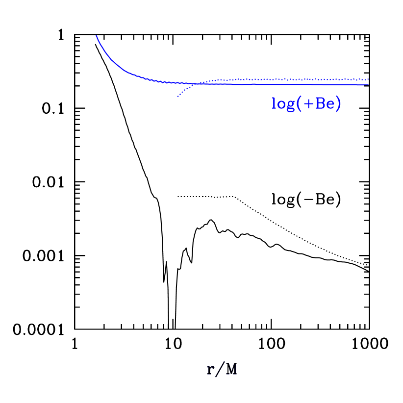
Figure 1: The initial (dotted) and final (solid) midplane Bernoulli parameters, $Be$, of two GRMHD accretion simulations. The Bernoulli parameter is measured in units of rest mass energy. The energetically unbound flow (blue) is the A0.0BtN10 model of McKinney et al. (2012). The energetically bound flow (black) is the ADAF/SANE model of Narayan et al. (2012). The unbound simulation reached $t=96,796M$ and the bound simulation reached $t=200,000M$. In both cases, the final $Be$ appears to depend on the initial $Be$.

2 New torus solution

We consider a fluid torus in hydrostatic equilibrium around a Kerr black hole. We assume the flow is axisymmetric and stationary. We use an ideal gas equation of state and assume the fluid has a constant entropy. Self-gravity is ignored.

We work in Boyer-Lindquist coordinates $\left(t,r,\theta,\phi\right)$ and units for which $G=c=1$. The solution is a function of $r$ and $\theta$ only (i.e., it is stationary and axisymmetric). There are six adjustable parameters. They are defined below but may be summarized here: $r_{in}$ is the radius of the inner edge of the torus, $r_{1}$ and $r_{2}$ control the shape of the angular momentum distribution, $\xi$ controls the rotation rate, $\kappa$ sets the entropy, and $\Gamma$ is the adiabatic index.

The components of the Kerr metric we need are

$$g_{tt} =-1+2Mr/\Sigma,\quad g_{t\phi}=-2Mar\sin^{2}\theta/\Sigma,$$ (1)

$$g_{\phi\phi} =\left[r^{2}+a^{2}\left(1+2Mr\sin^{2}\theta/\Sigma\right)\right]\sin^{2}\theta,$$ (2)

where $M$ and $a$ are the mass and spin of the black hole and $\Sigma=r^{2}+a^{2}\cos^{2}\theta$.

Let $u^{\mu}$ be the fluid four-velocity. We assume the fluid’s angular momentum density, $\ell\equiv u_{\phi}/|u_{t}|$, is constant on von Zeipel cylinders (Abramowicz, 1971). The radius, $\lambda$, of a von Zeipel cylinder with angular momentum $\ell$ is (Chakrabarti, 1985):

$$\lambda^{2}=-\ell(\lambda)\frac{\ell(\lambda)g_{t\phi}+g_{\phi\phi}}{\ell(\lambda)g_{tt}+g_{t\phi}}.$$ (3)

In Newtonian gravity, $\lambda=r\sin{\theta}$, the usual cylindrical radius. In the Schwarzschild metric, $\lambda=\sqrt{-g_{\phi\phi}/g_{tt}}$. In the Kerr metric, one must solve equation (3) numerically.

The angular momentum density of circular, equatorial orbits in the Kerr metric is (Novikov & Thorne, 1973)

$$\ell_{K}(r)\equiv u_{\phi}/|u_{t}|=\sqrt{Mr}\thinspace\mathcal{F}/\mathcal{G},$$ (4)

where,

$$\mathcal{F} =1-2a_{*}/r_{*}^{3/2}+a_{*}^{2}/r_{*}^{2},\quad\mathcal{G}=1-2/r_{*}+a_{*}/r_{*}^{3/2},$$

$$r_{*} =r/M,\quad a_{*}=a/M.$$

We choose the angular momentum distribution of the fluid torus to be:

$$\ell(\lambda)=\begin{cases}\xi\ell_{K}(\lambda_{1})&\mbox{if }\lambda<\lambda_{1}\\ \xi\ell_{K}(\lambda)&\mbox{if }\lambda_{1}<\lambda<\lambda_{2}\\ \xi\ell_{K}(\lambda_{2})&\mbox{if }\lambda>\lambda_{2}.\end{cases}$$ (5)

There are three regions. In the inner and outer regions of the torus, the angular momentum density is a constant independent of radius. The size of these regions is set by $\lambda_{1}$ and $\lambda_{2}$. At intermediate radii, the angular momentum density is a fraction $\xi$ of the Keplerian distribution (4). This is chosen to be close to the expected, sub-Keplerian angular momentum distribution of a real accretion flow. It is more physical than the power law angular momentum distributions of the Fishbone & Moncrief (1976) and Chakrabarti (1985) solutions.

The angular velocity of the torus is

$$\Omega\equiv\frac{u^{\phi}}{u^{t}}=-\frac{g_{t\phi}+\ell g_{tt}}{g_{\phi\phi}+\ell g_{t\phi}}.$$ (6)

We have assumed $u^{r}=u^{\theta}=0$, so this fully determines the velocity.

Given the velocity of the torus, we can determine its density and pressure from the Euler equation. Let

$$A\equiv u^{t}=\left(-g_{tt}-2\Omega g_{t\phi}-\Omega^{2}g_{\phi\phi}\right)^{-1/2},$$ (7)

which sets the gravitational force felt by the fluid. The Euler equation (Abramowicz et al., 1978) is then

$$\frac{\nabla p}{\rho_{0}+U+p}=\nabla\ln A-\frac{\ell\nabla\Omega}{1-\Omega\ell}.$$ (8)

Our notation is standard: $\rho_{0}$, $U$, and $p$ are the mass density, internal energy, and gas pressure of the fluid in its rest frame. Euler’s equation describes the balance between pressure gradients (LHS) and gravitational and centrifugal forces (RHS) required for hydrostatic equilibrium.

To solve the Euler equation, it is helpful to introduce the effective potential (Kozlowski et al., 1978)

$$W(r,\theta)\equiv-\ln(FA),$$ (9)

where,

$$\ln F(r,\theta)\equiv-\int_{r_{in}}^{r_{\rm\lambda m}(r,\theta)}{\frac{d\Omega}{dr}\frac{\ell dr}{1-\Omega\ell}}.$$ (10)

The lower limit of the integral, $r_{in}$, is the radius of the inner edge of the torus. The upper limit, $r_{\lambda m}(r,\theta)$, is the equatorial radius of the Von Zeipel cylinder containing $(r,\theta)$. For example, $r_{\lambda m}(r,\pi/2)=r$.

In terms of the effective potential, the Euler equation is

$$\frac{\nabla p}{\rho_{0}+U+p}=-\nabla W.$$ (11)

We can compute the effective potential because it depends only on $\ell$. So the RHS is known. The boundary of the torus is the isopotential surface $W(r,\theta)=W_{in}\equiv W(r_{in},\pi/2)$.

The specific enthalpy is $w=1+\epsilon+p/\rho_{0}$, where $\epsilon=U/\rho_{0}$ is the specific internal energy. For an isentropic torus, the Euler equation can be integrated to obtain (Kozlowski et al., 1978)

$$w(r,\theta)=e^{-\left(W(r,\theta)-W_{in}\right)}.$$ (12)

We assume the equation of state $p=\rho_{0}\epsilon(\Gamma-1)$, so the specific internal energy is

$$\epsilon=(w-1)/\Gamma.$$ (13)

The rest mass density and pressure are

$$\rho_{0} =\left[(\Gamma-1)\epsilon/\kappa\right]^{1/\left(\Gamma-1\right)},$$ (14)

$$p =\kappa\rho_{0}^{\Gamma}.$$ (15)

The entropy, $\kappa$, is a free parameter. The torus is now fully determined.

To summarize, we first choose the angular momentum distribution (5). The angular momentum distribution determines the angular velocity and effective potential. The effective potential determines the enthalpy of the torus through Euler’s equation. Fixing an ideal gas equation of state and assuming an isentropic torus, gives the density, pressure, and internal energy. There are six free parameters: the radius of the inner edge of the torus, $r_{in}$, the break radii in the angular momentum distribution, $r_{1}$ and $r_{2}$, the normalization of the angular momentum, $\xi$, the entropy, $\kappa$, and the adiabatic index, $\Gamma$. The entropy simply sets the density scale (equation 15) and, as there is no self-gravity, it has no effect on the dynamics.

3 Approximate analytical formulae

The solution of §2 can be implemented in GRMHD codes numerically. However, for physical understanding, it is useful to have approximate formulae that describe the torus analytically. In this section, we obtain approximate analytical formulae for the outer edge, pressure maximum, geometrical thickness, and Bernoulli parameter of the torus.

The most complicated feature of the exact solution is the integral in equation (10). To obtain approximate analytical formulae for the torus, we need to simplify this integral. Let us first rewrite it as

$$F=\left(1-\Omega\ell\right)\exp\left(\int_{r_{in}}^{r_{\lambda m}}\frac{\Omega}{1-\Omega\ell}\frac{d\ell}{dr}dr\right),$$ (16)

where we have used $\ell d\Omega=d(\Omega\ell)-\Omega d\ell$.

In the inner region of the torus ($\lambda<\lambda_{1}$), the angular momentum is constant and the integrand in equation (16) vanishes. So

$$F(r,\theta)=1-\Omega(r,\theta)\ell(r,\theta),\quad(\lambda<\lambda_{1}).$$ (17)

In the outer region of the torus ($\lambda>\lambda_{2}$), we may approximate the integral by plugging the Newtonian formula $\ell_{K}(\lambda)=\sqrt{M\lambda}$ into equation (5), and using the Newtonian angular velocity $\Omega(\lambda)=\ell(\lambda)/\lambda^{2}$. Now integrating from $\lambda_{1}$ to $\lambda_{2}$, we obtain

$$F\approx\left(1-\Omega\ell\right)I,\quad(\lambda>\lambda_{2}),$$ (18)

where,

$$I\equiv\left(\frac{1-\xi^{2}/\lambda_{2}}{1-\xi^{2}/\lambda_{1}}\right)^{1/2}.$$ (19)

Equation (18) is approximate because we ignored special relativistic contributions to $\ell$ and $\Omega$. But these are small in the outer regions of the torus. We can use our analytical approximation of $F$ to obtain simple formulae describing the torus.

3.1 Radius of the outer edge

The boundary of the torus is the isopotential surface $W(r,\theta)=W_{in}=W(r_{in},\pi/2)$. We can simplify $W$ at the outer edge by using a Newtonian description there. The equation for the outer radius, $r_{out}$, becomes

$$W_{in}\approx-\frac{M}{r_{out}}+\frac{\xi^{2}Mr_{2}}{2r_{out}^{2}}-\ln I.$$ (20)

The solution for the outer radius is

$$r_{out}/M\approx\frac{1+\sqrt{1-\xi^{2}\lambda_{2}\varpi}}{\varpi},$$ (21)

where

$$\varpi\equiv 2\ln\left[\frac{A}{I}\left(1-\frac{\ell^{2}}{\lambda^{2}}\right)\right]_{r=r_{in}}.$$ (22)

Figure 2 (top left panel) shows the variation of $r_{out}$ with $\xi$ for several choices of $r_{in}$ and fixed $r_{1}=42M$ and $r_{2}=1000M$. The outer radius increases as the inner radius decreases because the boundary of the torus is moving to larger isopotential surfaces. In the region of parameter space shown in Figure 2, the Bernoulli parameter is small and negative, as we will see below. When the Bernoulli parameter is small and negative, the outer radius is very sensitive to $\xi$.

Solutions with positive Bernoulli parameter have $r_{out}$ at infinity. They are unbound and not very physical. In fact, they are not even tori, they are infinite cylinders kept confined by a nonzero pressure at infinity. Unphysical, infinite cylinders based on the Fishbone & Moncrief (1976) and Chakrabarti (1985) solutions have at times been used as the initial condition for GRMHD simulations.

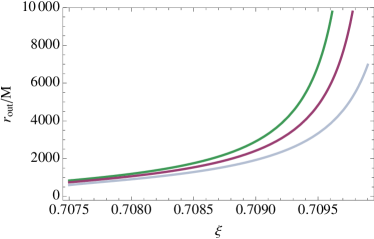
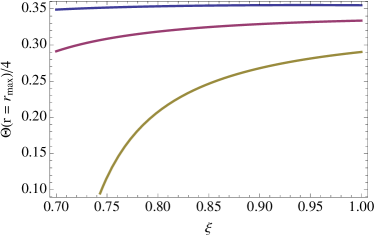
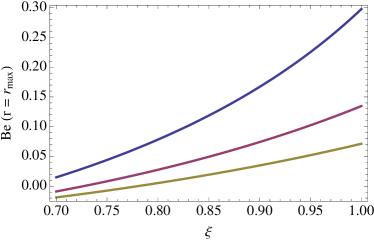
Figure 2: Counterclockwise from the upper left panel, we show the radius of the outer edge of the torus, the radius of the pressure maximum, the Bernoulli parameter at the pressure maximum, and the geometrical thickness at the pressure maximum as a function of the rotation parameter, $\xi$, for several choices of $r_{in}/M$: 8 (blue), 9.993 (green), 10 (red), 10.01 (gray), and 12 (yellow). The pressure maximum position, $r_{max}/M$, is independent of $r_{in}$. The horizontal scale of the upper left panel is different from the other panels because $r_{out}$ is only finite when $Be<0$.

3.2 Pressure maximum

The pressure gradient in the Euler equation (8) is zero at the pressure maximum. So the fluid must move along geodesics there. In other words, the pressure maximum is where

$$\ell(r_{max})=\ell_{K}(r_{max}),$$ (23)

where $\ell_{K}$ is the angular momentum of circular, equatorial geodesics (equation 4) and $r_{max}$ is the radius of the pressure maximum. For sub-Keplerian flow ($\xi<1$), the pressure maximum must be in the inner region of the torus ($\lambda<\lambda_{1}$), because the angular momentum is strictly sub-Keplerian for $\lambda>\lambda_{1}$.

Equation (23) gives

$$r_{max}(\xi,\lambda_{1})\approx\xi^{2}\ell_{K}(\lambda_{1})^{2}-4M,$$ (24)

where $-4M$ is the leading order relativistic correction. Figure 2 (lower left panel) shows the dependence of $r_{max}$ on $\xi$ for $\lambda_{1}=42M$. In the Keplerian limit $\xi\rightarrow 1$, the pressure maximum approaches $\lambda_{1}$. Lowering $\xi$ moves the pressure maximum toward the inner edge of the torus.

3.3 Bernoulli parameter

The relativistic Bernoulli parameter is (Novikov & Thorne, 1973)

$$Be=-u_{t}w-1.$$ (25)

Tori with $Be>0$ are energetically unbound and tori with $Be<0$ are energetically bound. In the inner region of the torus ($\lambda<\lambda_{1}$), the Bernoulli parameter is:

$$Be=-(g_{tt}+g_{t\phi}\Omega)\frac{A^{2}(1-\Omega\ell)}{\left[A(1-\Omega\ell)\right]_{r=r_{in}}}-1.$$ (26)

Figure 2 (lower right panel) shows how $Be(r_{max})$ depends on $\xi$ for several choices of $r_{\rm in}$ and fixed break radii $r_{1}=42M$ and $r_{2}=1000M$. The outer edge of the torus goes to infinity as $Be\rightarrow 0$ (from below).

3.4 Thickness

The boundary of the torus is the isopotential surface $W(r,\theta)=W_{in}$. In the inner region of the torus ($\lambda<\lambda_{1}$), the surface of the torus is

$$\sin\theta=-g_{tt}\frac{\ell^{2}}{r^{2}}\frac{1}{1+g_{tt}\left[A\left(1-\Omega\ell\right)\right]_{r=r_{in}}}.$$ (27)

$\theta$ is measured from the the polar axis, so the scale height of the torus is $\Theta=\pi/2-\theta$. Figure 2 (upper right panel) shows $\Theta(r_{max})$ as a function of $\xi$ for several choices of $r_{in}$.

3.5 Bernoulli parameter and thickness

Our solutions tend to be more bound than earlier solutions. We show this with an example. Figure 3 (upper left panel) shows the Bernoulli parameter of one of our solutions in the $(r,\theta)$ plane. The torus is energetically bound: $Be<0$. In the same figure (upper right panel), we show the Bernoulli parameter of a solution of Chakrabarti (1985). This torus is energetically unbound.

In the bottom panels of Figure 3, we show the density scale heights,

$$|h/r|=\frac{\int\left|\theta-\pi/2\right|\rho_{0}\sqrt{-g}d\theta d\phi}{\int\rho_{0}\sqrt{-g}d\theta d\phi},$$ (28)

of both solutions. Thinner tori tend to be more bound than thicker tori, but in this example the unbound torus is actually thinner than the bound torus. In other words, our solutions tend to be more bound than earlier solutions. This is an advantage, because unbound solutions are unphysical as initial conditions for GRMHD simulations. They are infinitely extended cylinders supported by pressure at infinity.

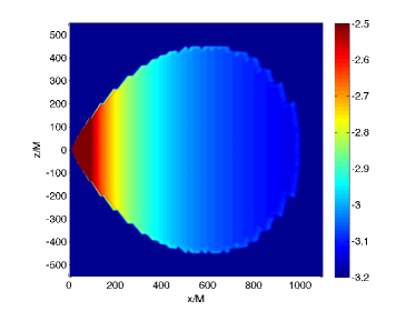
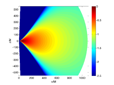
Figure 3: The panels in the left column show $\log(-Be)$ and $|h/r|$ for the new equilibrium torus solution described in the text. The Bernoulli parameter is shown as a function of $(r,\theta)$ and as a function of $r$ at the midplane. The torus is energetically bound, i.e., $Be<0$. The panels in the right column show $\log(Be)$ and $|h/r|$ for a solution of Chakrabarti (1985) which is energetically unbound, i.e., $Be>0$. Note that the unbound torus is actually thinner than the bound torus in this example.

A second lesson to draw from this example is that the torus thickness, $|h/r|$, does not fix even the sign of the Bernoulli parameter (much less its value). GRMHD simulators typically focus on the thickness of the initial torus but this may not be enough if, for example, the Bernoulli parameter influences the strength of accretion disk winds. In other words, it may be important to know the thickness and the Bernoulli parameter of the initial torus independently.

4 Conclusions

We have constructed a new equilibrium torus solution. It provides an alternative initial condition for GRMHD disk simulations to the earlier solutions of Fishbone & Moncrief (1976) and Chakrabarti (1985). The angular momentum density is constant in the inner and outer regions of the torus and follows a sub-Keplerian distribution in between. The entropy is constant everywhere.

The Bernoulli parameter, rotation rate, and geometrical thickness of the solution can be varied independently. The torus tends to be more energetically bound than earlier solutions, for the same thickness $|h/r|$. In fact, we have shown that it is possible to generate equilibrium tori with the same $|h/r|$, but for which one is bound and the other unbound. So as GRMHD initial conditions, the new solutions might lead to weaker (or non-existent) disk winds. Future GRMHD simulations will need to explore how the simulation results depend on the Bernoulli parameter, rotation rate, and geometrical thickness of the initial equilibrium torus.

In real accretion flows, the Bernoulli parameter is probably set at the outer edge of the flow. If this is far from the black hole (for example, at the Bondi radius), then one expects $Be\sim 0$. It is not possible to obtain converged GRMHD simulations out to the Bondi radius. One would need to run the simulations for a timescale of order the Bondi radius viscous time, which is impractical. Computational resources limit the duration of even the longest run simulations to $t\sim 200,000M$, which corresponds to the viscous time at $r\sim 200M$. Probably the best one can hope to do is choose an initial condition with a realistic Bernoulli parameter ($Be\sim 0$) at the outset. The solution in this paper is flexible enough to allow independent control over the thickness and Bernoulli parameter of the torus, so it is an ideal initial condition for GRMHD simulations. In fact, while this paper was in preparation, there appeared several simulations based on our solution (Narayan et al., 2012; Sa̧dowski et al., 2013; Penna et al., 2013a, b). We expect more soon.

Appendix A Adding a magnetic field

Implementing the new equilibrium torus as a GRMHD initial condition requires adding a magnetic field to the torus. Here we record one possible magnetic field, a series of poloidal magnetic loops. We discuss the Bernoulli parameter of the magnetized torus in §A.2.

A.1 Magnetic field solution

We construct the magnetic field so that each loop carries the same magnetic flux and $\beta=p_{\rm gas}/p_{\rm mag}$ is roughly constant. Simulations often require initial conditions that minimize secular variability during the run, so these features can be useful.

Three free parameters appear in the solution: $r_{\rm start}$, $r_{\rm end}$, and $\lambda_{B}$. The first two set the inner and outer boundaries of the magnetized region and the third controls the size of the poloidal loops.

We define the field through the vector potential, $A_{\mu}$. The magnetic loops are purely poloidal, so only $A_{\phi}$ is nonzero. To keep $\beta$ close to a constant, the magnetic field strength tracks the fluid’s internal energy density. Define

$$q=\begin{cases}\sin^{3}\theta\left(U_{c}/U_{cm}-0.2\right)/0.8&\mbox{if }r_{\rm start}<r<r_{\rm end}\\ 0&\text{otherwise, }\end{cases}$$ (29)

where,

$$U_{c}(r,\theta) =U(r,\theta)-U(r_{\rm end},\pi/2),$$ (30)

$$U_{cm}(r) =U(r,\pi/2)-U(r_{\rm end},\pi/2).$$ (31)

The function $q$ is defined to give $q=1$ at the midplane and $q\rightarrow 0$ away from the midplane. The factor $\sin^{3}\theta$ smooths the vector potential as it approaches the edges of the torus. Dropping this factor leads to a torus with highly magnetized edges.

Further define

$$f(r)=\lambda_{B}^{-1}\left(r^{2/3}+15r^{-2/5}/8\right).$$ (32)

The vector potential is then

$$A_{\phi} =\begin{cases}q\sin\left(f(r)-f(r_{\rm start})\right)&\mbox{if }q>0\\ 0&\mbox{otherwise},\end{cases}$$ (33)

all other $$A_{\mu}$$=0. (34)

The sinusoidal factor in $A_{\phi}$ breaks the poloidal field into a series of loops. The function $f(r)$ gives each loop the same magnetic flux. The number of loops is controlled by $\lambda_{B}$. The overall normalization of $A_{\phi}$ has not been specified so it can be tuned to give any field strength.

We give an example in Figure 4. The equilibrium torus is as in Figure 3 and the field parameters are $r_{\rm start}=25$, $r_{\rm end}=550$, and $\lambda_{B}=15/4$. In this example there are eight magnetic loops. The magnetic flux, $A_{\phi}$, peaks at the center of each loop, measures the flux carried by the loop, and is the same across the torus. The magnetization $\beta=p_{\rm gas}/p_{\rm mag}$ peaks at loop edges and drops at loop centers, but is roughly constant across the torus. In this example $\beta\sim 100$.

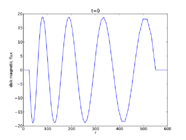
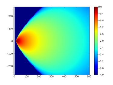
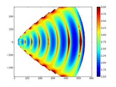
Figure 4: The top two panels show the mid-plane density and the enclosed magnetic flux as a function of radius. The lower two panels show the density and the magnetization parameter $\beta$ of the torus in the poloidal plane. Each loop carries the same magnetic flux. The magnetization is roughly constant throughout the torus.

A.2 GRMHD Bernoulli parameter

The stress energy tensor of a magnetized fluid is

$$T_{\mu\nu}=\left(\rho_{0}+U+\frac{b^{2}}{2}\right)u_{\mu}u_{\nu}+\left(p_{\rm gas}+\frac{b^{2}}{2}\right)h_{\mu\nu}-b_{\mu}b_{\nu},$$

where $b_{\mu}$ is the magnetic field in the fluid’s rest frame and $h_{\mu\nu}=g_{\mu\nu}+u_{\mu}u_{\nu}$ is the projection tensor. The magnetic field contributes $b^{2}/2$ to the total internal energy and $b^{2}/2$ to the total pressure, and introduces a stress term, $-b_{\mu}b_{\nu}$.

The Euler equations, $h\cdot\left(\nabla\cdot T\right)=0$, become:

$$\left(\rho_{0}+U+p_{\rm gas}+b^{2}\right)a=-h\cdot\nabla\left(p_{\rm gas}+\frac{b^{2}}{2}\right)h-h\cdot\left(b\cdot\nabla\right)b,$$

where $a=\nabla_{u}u$ is the fluid’s acceleration. We have used $\nabla\cdot b=0$ to simplify the last term on the RHS.

Assume the flow is stationary and adiabatic, project the Euler equations along $\xi=\partial_{t}$, and combine terms using the first law of thermodynamics. This leads to:

$$\frac{d}{d\tau}\left(\frac{\rho_{0}+U+p_{\rm gas}+b^{2}}{\rho_{0}}u_{t}\right)=-\frac{1}{\rho_{0}}\xi\cdot h\cdot\left(b\cdot\nabla\right)b.$$

For the field configuration of §A.1, $b$ is purely poloidal and $\xi\cdot h$ is purely toroidal. So the RHS is zero.

We thus obtain a straightforward generalization of equation (25):

$$Be=-\left(1+\frac{U+p_{\rm gas}+b^{2}}{\rho_{0}}\right)u_{t}-1.$$ (35)

The unmagnetized torus has $Be\sim-w_{\rm gas}$. Adding magnetic fields to the torus, with gas-to-magnetic pressure ratio $\beta=p_{\rm gas}/p_{\rm mag}$, changes the Bernoulli parameter by terms of order $1/\beta$. Simulations typically have initial $\beta\sim 100$, in which case the magnetic contribution to the Bernoulli parameter is of order $1\%$.

References

- Abramowicz et al. (1978) Abramowicz M., Jaroszynski M., Sikora M., 1978, A&A, 63, 221
- Abramowicz (1971) Abramowicz M. A., 1971, Acta Astron., 21, 81
- Balbus & Hawley (1991) Balbus S. A., Hawley J. F., 1991, ApJ, 376, 214
- Balbus & Hawley (1998) Balbus S. A., Hawley J. F., 1998, Reviews of Modern Physics, 70, 1
- Barkov (2008) Barkov M. V., 2008, in American Institute of Physics Conference Series, edited by M. Axelsson, vol. 1054 of American Institute of Physics Conference Series, 79–85
- Barkov & Baushev (2011) Barkov M. V., Baushev A. N., 2011, New A, 16, 46
- Beckwith et al. (2008) Beckwith K., Hawley J. F., Krolik J. H., 2008, ApJ, 678, 1180
- Chakrabarti (1985) Chakrabarti S. K., 1985, ApJ, 288, 1
- De Villiers et al. (2003) De Villiers J., Hawley J. F., Krolik J. H., 2003, ApJ, 599, 1238
- Dibi et al. (2012) Dibi S., Drappeau S., Fragile P. C., Markoff S., Dexter J., 2012, MNRAS, 426, 1928
- Farris et al. (2012) Farris B. D., Gold R., Paschalidis V., Etienne Z. B., Shapiro S. L., 2012, Physical Review Letters, 109, 22, 221102
- Farris et al. (2011) Farris B. D., Liu Y. T., Shapiro S. L., 2011, Phys. Rev. D, 84, 2, 024024
- Fishbone (1977) Fishbone L. G., 1977, ApJ, 215, 323
- Fishbone & Moncrief (1976) Fishbone L. G., Moncrief V., 1976, ApJ, 207, 962
- Fragile & Blaes (2008) Fragile P. C., Blaes O. M., 2008, ApJ, 687, 757
- Fragile et al. (2007) Fragile P. C., Blaes O. M., Anninos P., Salmonson J. D., 2007, ApJ, 668, 417
- Gammie et al. (2004) Gammie C. F., Shapiro S. L., McKinney J. C., 2004, ApJ, 602, 312
- Henisey et al. (2012) Henisey K. B., Blaes O. M., Fragile P. C., 2012, ApJ, 761, 18
- Hilburn et al. (2010) Hilburn G., Liang E., Liu S., Li H., 2010, MNRAS, 401, 1620
- Kozlowski et al. (1978) Kozlowski M., Jaroszynski M., Abramowicz M. A., 1978, A&A, 63, 209
- McKinney (2005) McKinney J. C., 2005, arXiv:astro-ph/0506369
- McKinney (2006) McKinney J. C., 2006, MNRAS, 368, 1561
- McKinney et al. (2012) McKinney J. C., Tchekhovskoy A., Blandford R. D., 2012, MNRAS, 423, 3083
- Mościbrodzka et al. (2011) Mościbrodzka M., Gammie C. F., Dolence J. C., Shiokawa H., 2011, ApJ, 735, 9
- Nagataki (2009) Nagataki S., 2009, ApJ, 704, 937
- Narayan et al. (2012) Narayan R., Sadowski A., Penna R. F., Kulkarni A. K., 2012, MNRAS, 426, 3241
- Noble et al. (2009) Noble S. C., Krolik J. H., Hawley J. F., 2009, ApJ, 692, 411
- Noble et al. (2007) Noble S. C., Leung P. K., Gammie C. F., Book L. G., 2007, Classical and Quantum Gravity, 24, 259
- Novikov & Thorne (1973) Novikov I. D., Thorne K. S., 1973, in Black Holes (Les Astres Occlus), edited by C. Dewitt, B. S. Dewitt, 343–450
- Penna et al. (2010) Penna R. F., McKinney J. C., Narayan R., Tchekhovskoy A., Shafee R., McClintock J. E., 2010, MNRAS, 408, 752
- Penna et al. (2013a) Penna R. F., Narayan R., Sa̧dowski A., 2013a, MNRAS submitted, arxiv:1307.4752
- Penna et al. (2013b) Penna R. F., Sa̧dowski A., Kulkarni A. K., Narayan R., 2013b, MNRAS, 428, 2255
- Sa̧dowski et al. (2013) Sa̧dowski A., Narayan R., Penna R. F., Zhu Y., 2013, MNRAS submitted, arxiv:1307.1143
- Shafee et al. (2008) Shafee R., McKinney J. C., Narayan R., Tchekhovskoy A., Gammie C. F., McClintock J. E., 2008, ApJ, 687, L25
- Shcherbakov et al. (2012) Shcherbakov R. V., Penna R. F., McKinney J. C., 2012, ApJ, 755, 133
- Shibata et al. (2007) Shibata M., Sekiguchi Y. I., Takahashi R., 2007, Progress of Theoretical Physics, 118, 257
- Shiokawa et al. (2012) Shiokawa H., Dolence J. C., Gammie C. F., Noble S. C., 2012, ApJ, 744, 187
- Tchekhovskoy & McKinney (2012) Tchekhovskoy A., McKinney J. C., 2012, MNRAS, 423, L55
- Tchekhovskoy et al. (2011) Tchekhovskoy A., Narayan R., McKinney J. C., 2011, MNRAS, 418, L79