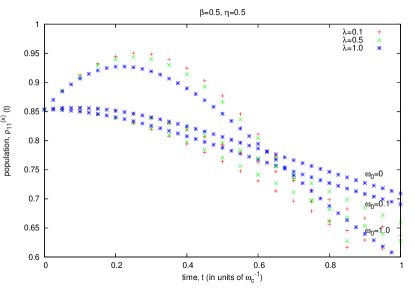
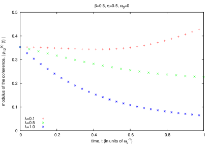
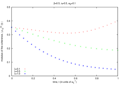
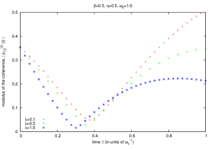
Efficient finite-time measurements under thermal regimes

Carlos Alexandre Brasil Instituto de Física "Gleb Wataghin", Universidade Estadual de Campinas, P.O. Box 6165, 13083-970 Campinas, SP, Brazil    Leonardo Andreta de Castro    Reginaldo de Jesus Napolitano Instituto de Física de São Carlos, Universidade de São Paulo, P.O. Box 369, 13560-970 São Carlos, SP, Brazil
Abstract

Contrary to conventional quantum mechanics, which treats measurement as instantaneous, here we explore a model for finite-time measurement. The main two-level system interacts with the measurement apparatus in a Markovian way described by the Lindblad equation, and with an environment, which does not include the measuring apparatus. To analyse the environmental effects on the final density operator, we use the Redfield approach, allowing us to consider a non-Markovian noise. In the present hybrid theory, to trace out the environmental degrees of freedom, we use a previously-developed analytic method based on superoperator algebra and Nakajima-Zwanzig superoperators. Here, we analyse two types of system-environment interaction, phase and amplitude damping, which allows us to conclude that, in general, a finite-time quantum measurement performed during a certain period is more efficient than an instantaneous measurement performed at the end of it, because the rate of change of the populations is attenuated by the system-measurement apparatus interaction.

pacs:
03.65.Yz 03.65.Ta 02.60.-x

I Introduction

The measurement problem in quantum mechanics is responsible for most of the controversy surrounding this theory key-5-1 ; key-6 . While in classical physics the observation of an object does not presuppose any changes of its properties, in quantum mechanics this interaction, far from insignificant, causes profound changes on the object under observation. Besides changing the state of the system, the measurement of a given property can influence the value of another (the case of conjugate observables such as position and momentum). Another aggravating aspect is the fact that it is not possible to predict with certainty the result of a specific measurement: quantum mechanics rules allow us to know only the several possible results and their respective probabilities - it is an ensemble theory, as found by Born key-7 ; key-8 and Dirac key-9 ; key-10 .

To describe a measurement, it is necessary to expand the wave-function in terms of the eigenstates of the observable to be measured: the possible results of the measurement will be the respective eigenvalues of the observable, and the corresponding probabilities will be the square modulus of the expansion coefficients. When the measurement is complete, the wave-function reduction takes place, and the state of the system is projected into the eigenstate corresponding to the eigenvalue obtained. All this was synthesized by von Neumann in his pioneer treatise on quantum mechanics key-4 , where he states the two possible processes of wave function evolution:

  1. 1.

    Reduction, when a measurement is made;

  2. 2.

    Unitary evolution according to the Schrödinger equation, between measurements.

In von Neumann’s original work key-4 , the transmission of information to the measuring apparatus is described by considering two Hilbert spaces which we shall call I𝐼I, the principal system under observation, and II𝐼𝐼II, the measurement apparatus. Here, let A^(I)superscript^𝐴𝐼\hat{A}^{\left(I\right)} be the observable of I𝐼I to be measured, {|an}ketsubscript𝑎𝑛\left\{\left|a_{n}\right\rangle\right\} the set of its eigenfunctions with associated eigenvalues ansubscript𝑎𝑛a_{n}, and let |ϕ(I)ketsuperscriptitalic-ϕ𝐼\left|\phi^{\left(I\right)}\right\rangle be the initial state of the system, given as the linear combination

|ϕ(I)=𝑛cn|an.ketsuperscriptitalic-ϕ𝐼𝑛subscript𝑐𝑛ketsubscript𝑎𝑛\left|\phi^{\left(I\right)}\right\rangle=\underset{n}{\sum}c_{n}\left|a_{n}\right\rangle. (1)

Obviously, |an|ϕ(I)|2superscriptinner-productsubscript𝑎𝑛superscriptitalic-ϕ𝐼2\left|\left\langle a_{n}|\phi^{\left(I\right)}\right\rangle\right|^{2} is the probability to find ansubscript𝑎𝑛a_{n} as the possible result of the measurement. Considering that the measurement results for apparatus II𝐼𝐼II are shown on a scale of values, we define an observable B^(II)superscript^𝐵𝐼𝐼\hat{B}^{\left(II\right)} that gives us the pointer position of the eingenvalue bnsubscript𝑏𝑛b_{n} (referring to the eigenstate |bnketsubscript𝑏𝑛\left|b_{n}\right\rangle). In this case, there is a direct correlation between ansubscript𝑎𝑛a_{n} and bnsubscript𝑏𝑛b_{n}: the result of the measurement of B^(II)superscript^𝐵𝐼𝐼\hat{B}^{\left(II\right)} over II𝐼𝐼II will give bnsubscript𝑏𝑛b_{n} only if the result of the measurement of A^(I)superscript^𝐴𝐼\hat{A}^{\left(I\right)} over I𝐼I gives ansubscript𝑎𝑛a_{n}.

Next, let us define the initial state |ϕ(I)ketsuperscriptitalic-ϕ𝐼\left|\phi^{\left(I\right)}\right\rangle of I𝐼I - unknown in the sense of its being a linear combination of eigenstates of A^(I)superscript^𝐴𝐼\hat{A}^{\left(I\right)} (the goal of the measurement is to determine the state) - and the initial state |ϕ(II)ketsuperscriptitalic-ϕ𝐼𝐼\left|\phi^{\left(II\right)}\right\rangle of II𝐼𝐼II, denoted, for simplicity, by |b0ketsubscript𝑏0\left|b_{0}\right\rangle. The initial state of the combined system I+II𝐼𝐼𝐼I+II will then be

|ϕ(I+II)(0)=|ϕ(I)|ϕ(II),ketsuperscriptitalic-ϕ𝐼𝐼𝐼0tensor-productketsuperscriptitalic-ϕ𝐼ketsuperscriptitalic-ϕ𝐼𝐼\left|\phi^{\left(I+II\right)}\left(0\right)\right\rangle=\left|\phi^{\left(I\right)}\right\rangle\otimes\left|\phi^{\left(II\right)}\right\rangle, (2)

where

{|ϕ(I)=𝑛cn|an|ϕ(II)=|b0.casesketsuperscriptitalic-ϕ𝐼absent𝑛subscript𝑐𝑛ketsubscript𝑎𝑛ketsuperscriptitalic-ϕ𝐼𝐼absentketsubscript𝑏0\begin{cases}\left|\phi^{\left(I\right)}\right\rangle&=\underset{n}{\sum}c_{n}\left|a_{n}\right\rangle\\ \left|\phi^{\left(II\right)}\right\rangle&=\left|b_{0}\right\rangle\end{cases}\>. (3)

For simplicity, the tensor-product\otimes symbol will be omitted from now on. The transmission of information from I𝐼I to II𝐼𝐼II will be made through the unitary operation - i.e., by the process 2 above - associated to the H^meas(I+II)superscriptsubscript^𝐻𝑚𝑒𝑎𝑠𝐼𝐼𝐼\hat{H}_{meas}^{\left(I+II\right)} Hamiltonian, which acts over the global system I+II𝐼𝐼𝐼I+II . If the measurement extends over a time interval τ𝜏\tau, the final global state will be

|ϕ(I+II)(τ)=eiH^meas(I+II)τ|ϕ(I+II)(0).ketsuperscriptitalic-ϕ𝐼𝐼𝐼𝜏superscript𝑒𝑖Planck-constant-over-2-pisuperscriptsubscript^𝐻𝑚𝑒𝑎𝑠𝐼𝐼𝐼𝜏ketsuperscriptitalic-ϕ𝐼𝐼𝐼0\left|\phi^{\left(I+II\right)}\left(\tau\right)\right\rangle=e^{-\frac{i}{\hbar}\hat{H}_{meas}^{\left(I+II\right)}\tau}\left|\phi^{\left(I+II\right)}\left(0\right)\right\rangle. (4)

At this point, von Neumann defines the unitary operator

Δ^eiH^meas(I+II)τ^Δsuperscript𝑒𝑖Planck-constant-over-2-pisuperscriptsubscript^𝐻𝑚𝑒𝑎𝑠𝐼𝐼𝐼𝜏\hat{\Delta}\equiv e^{-\frac{i}{\hbar}\hat{H}_{meas}^{\left(I+II\right)}\tau} (5)

to simplify his calculations. The question, then, is how to find a form for Δ^^Δ\hat{\Delta} that fits the established measurement criteria. This is a simple task and the result is

Δ^m,nxmn|am|bn=m,nxmn|am|bm+n.^Δ𝑚𝑛subscript𝑥𝑚𝑛ketsubscript𝑎𝑚ketsubscript𝑏𝑛𝑚𝑛subscript𝑥𝑚𝑛ketsubscript𝑎𝑚ketsubscript𝑏𝑚𝑛\hat{\Delta}\underset{m,n}{\sum}x_{mn}\left|a_{m}\right\rangle\left|b_{n}\right\rangle=\underset{m,n}{\sum}x_{mn}\left|a_{m}\right\rangle\left|b_{m+n}\right\rangle. (6)

It can be shown that applying (5) to (2) gives

|ϕ(I+II)(τ)=Δ^|ϕ(I+II)(0)=Δ^𝑛cn|an|b0=𝑛cn|an|bn.ketsuperscriptitalic-ϕ𝐼𝐼𝐼𝜏^Δketsuperscriptitalic-ϕ𝐼𝐼𝐼0^Δ𝑛subscript𝑐𝑛ketsubscript𝑎𝑛ketsubscript𝑏0𝑛subscript𝑐𝑛ketsubscript𝑎𝑛ketsubscript𝑏𝑛\left|\phi^{\left(I+II\right)}\left(\tau\right)\right\rangle=\hat{\Delta}\left|\phi^{\left(I+II\right)}\left(0\right)\right\rangle=\hat{\Delta}\underset{n}{\sum}c_{n}\left|a_{n}\right\rangle\left|b_{0}\right\rangle=\underset{n}{\sum}c_{n}\left|a_{n}\right\rangle\left|b_{n}\right\rangle.

The acquisition of information of the state is made by the process 1 above, with the results having associated probabilities |cn|2superscriptsubscript𝑐𝑛2\left|c_{n}\right|^{2} - Born’s rule.

In his work, von Neumann did not explicitly consider the time during which the measurement apparatus interacts with the system because the introduction of Δ^^Δ\hat{\Delta} eliminates the measurement time τ𝜏\tau from the calculations. A way to analyze this time period within the conventional structure of quantum mechanics as a statistical theory (and non causal in von Neumann’s point of view key-4 ) consists of considering the interaction between the system and the measurement apparatus evolving according to the Schrödinger equation or, more generally, the Liouville-von Neumann equation. In such an approach, we still have an equation for the density operator and, consequently, the probabilistic character of quantum mechanics is still present: the populations provide the associated probabilities for the possible results. Here, the problem of the wave-function reduction will not be analyzed and/or refuted - there are, indeed, interpretations of quantum mechanics where the reduction phenomenon is treated as nonexistent key-11 ; key-12 ; key-13 ; key-14 .

To clarify this treatment, it is convenient to use a framework that resembles the one by Peres key-15 , who labeled the procedure of acquiring information regarding the physical system as “intervention”. That procedure is divided into two parts: the measurement, when the apparatus interacts with the system and acquires the information, and the reading (or output), when the results of the intervention become known and the reduction of the wave function occurs. In the last step, the probabilistic information is contained in the populations of the density operator.

As mentioned previously, a more realistic description of the measurement apparatus implies the distinction between its microscopic and macroscopic degrees of freedom. To each possible eigenvalue measured, there is one and only one macroscopic value. However, this variable does not describe completely the state of the measurement apparatus, because there are many microscopic states corresponding to the same value of the macroscopic variable. As in the measurement the only important variable is the macroscopic one, we must take the partial trace over the microscopic variables. Under the Markov approximation for the interaction between the system and the measurement apparatus, this procedure leads to the Lindblad equation key-16 ; key-17 ; key-18 , where only the system coordinates appear. This equation for the density operator has a term for unitary evolutions (the Liouvillian, already known) and a second term, for the non-unitary evolutions, named Lindbladian. It is exactly the non-unitary term that allows us to introduce the time interval during the interaction between the system and the measurement apparatus key-19 . In the quantum-measurement-theory context, its derivation was sugested in key-15 and made in a simple manner in key-27 .

Until now, we have a situation where only two systems are considered: the system on which the measurement is made (which is the object of our interest), and the measurement apparatus. However, in real situations, the perfect isolation of the system is not always possible to achieve and, consequently, the environment perturbations change the final density operator in some way. To treat this situation, we consider that the system interacts with both the environment and the measurement apparatus, the effects of the environment being introduced in the Liouvillian of the Lindblad equation. In this way, with the partial trace over the environmental degrees of freedom, we obtain an equation in the Lindblad form, provided the environment is assumed as Markovian. To calculate the more general trace over the environmental degrees of freedom appearing in the Lindblad equation, we developed a formalism key-20 based on the superoperator algebra and the Nakajima-Zwanzig projectors key-21 ; key-22 .

It should be noted that alternative methods of describing continuous measurements that do not recur to the Lindblad superoperator exist, and include the introduction of an extra term to the Hamiltonian to account for the interaction with the measurement apparatus QZE , and the use of a stochastic master equation REVIEW . This latter description is not incompatible with the one provided by the Lindblad equation key-19 , which, for this choice of Lindblad operators, is also equivalent to the master equation for continuous position measurements derived by Barchielli et al. BARCHIELLI Our choice of employing the Lindblad equation as the starting point of our model, however, has proven satisfactory for the solution of the problem of the noisy finite-time measurement, that is, a finite-time measurement that occurs while the system suffers errors caused by an external environment. The investigation of this problem is what constitutes our original contribution to the field.

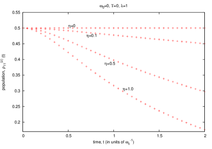
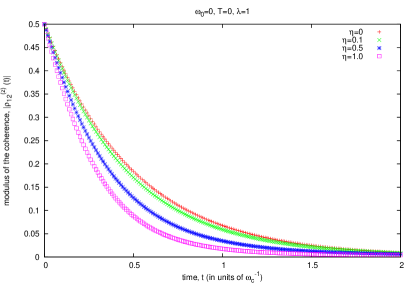
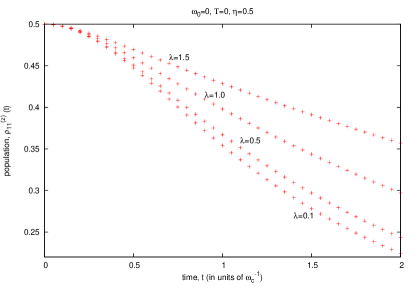
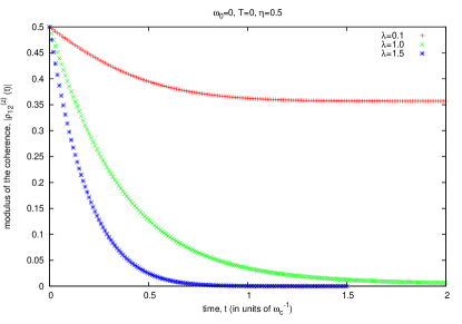
In previous papers key-20 ; key-23 ; key-24 , our formalism was applied to a two-state system in contact with an environment via phase-damping interaction, in the case of an Ohmic spectral density. Under some restrictions - both the natural system frequency and the environmental temperature set to zero - chosen to simplify the problem and allow analytical solutions, we verified that key-23 , when the measurement does not commute with the system-environment interaction, (i) the more intense the system-environment interaction, the more marked is the decrease of the population - i.e., the larger is the measurement error - and (ii) the more intense the system-measurement apparatus interaction, the less marked is the rate of change of the populations. From (ii), we concluded that finite-time measurements can be more efficient than instantaneous ones, when the measurement does not commute with the interaction between the system and the environment, because the nature of the system-apparatus interaction reduces the rate of change of the populations. To estimate the efficiency of a measurement, here, we adopt the criterion that an ideal measurement would consist of the instantaneous acquisition of information from the system before its state was altered by the environmental noise. If the populations of the system have been significantly altered by the time the measurement reaches its completion, the probabilities of encountering the apparatus’s pointer in either state will be visibly different from the probabilities associated with the initial state of the system measured, thus rendering the process inefficient. Next, analyzing the behavior of the coherences, which decrease with time, we established a criterion for the measurement duration key-24 .

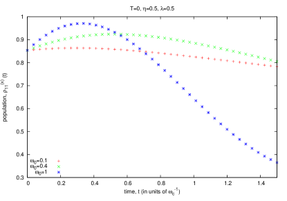
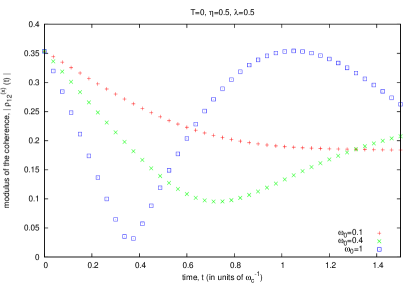
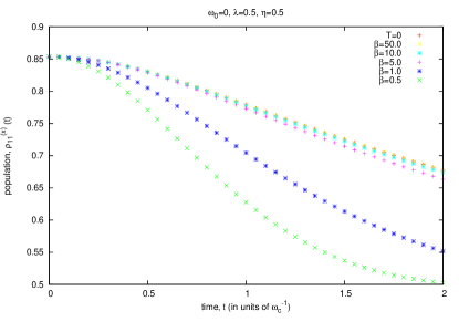
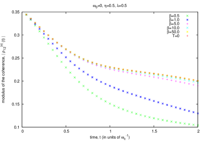
In the present work, we remove the restrictions and treat the interaction between the system and the environment as either the phase-damping or the amplitude-damping type, aiming at verifying, in a more general form, the influence of the environment on the final reduced density operator. We verify that, in general, the conclusions obtained in the previous works for state protection and system-environmental coupling apply to both interactions (phase and amplitude damping), even in the case of a finite environmental temperature. The addition of system frequency induces an oscillatory behavior on the populations. For the coherences, however, we observe that the introduction of the system frequency causes their modulus to approach, after a certain time interval, a constant asymptotic value, that may or may not be zero. Although we cannot, in this case, obtain a simple expression for the duration of the measurement, we still use the coherences to establish the time at which the system-environment interaction can be interrupted and the reading of the state accomplished - in this case, the time when the coherences assume the constant asymptotic value. Obviously, in more general cases, when the behavior of the system is not simple (the coherences no longer show a monotonic decrease), its physical properties must be considered to the establishment of the measurement time. Here, we do not change the spectral density and do not increase the number of states of the system under measurement - these extensions are left open and can be more safely developed under the light of the knowledge of the results presented here.

The possibility of application of this kind of measurement to improve the quality of the results depends, however, on the practical existence of measurements that can be performed during a finite period of time, in accordance with the model. There is, however, a recent application of our work - see ref. key-28 - in the context of Measurement-based Direct quantum Feedback Control (MDFC) key-29 ; key-30 .

This article is structured as follows: in Sec. II, we recapitulate our description of noisy finite-time measurements, providing the basis for the solutions obtained in Sec. III and Sec. IV, first for the phase-damping case, and then for the amplitude-damping one. Analyses of the solutions, together with graphs, are presented in Sec. V, conclusions and perspectives are given in Sec. VI. An appendix explains how this model of finite-time measurement could be experimentally tested against the more conservative approach that presupposes instantaneous measurements.

To present the results in a more logical and complete fashion, some of the contents of this article have been recapitulated from our previous works. Sec. II briefly explains the method that can be found, with greater details, on key-20 and solutions for the Lindblad equation for x-component measurement without environment found on key-23 ; Sec. III shows the z-component solution and the simplified (T=0𝑇0T=0 and ω0=0subscript𝜔00\omega_{0}=0) x-component solutions found on key-23 for the phase-damping interaction; finally, on Sec. V we show the formula for upper limit for the measurement duration found on key-24 . All the other results, however, are new.

II The Model of Finite-Time Measurement

In this section, we overview the model of noisy finite-time measurement that was developed and employed in our previous works key-23 ; key-24 . This model assumes that the system interacts with the measurement apparatus through a Markovian interaction. However, the finite nature of this description allows for other processes to occur before the measurement reaches its end.

In the usual treatment, when measurements are performed over the principal system S𝑆S, it is assumed that S𝑆S is perfectly isolated from the environment, interacting non-unitarily with the measurement apparatus. However, as we are considering the measurement as a finite-time process that may take a certain period to reach its completion, here we make the assumption that the system is not isolated, but also interacting with an environment B𝐵B. To deal with this situation, we describe the additional interaction between the system and the environment as a unitary evolution, with the Hamiltonian

H^=H^B+H^SB+H^S,^𝐻subscript^𝐻𝐵subscript^𝐻𝑆𝐵subscript^𝐻𝑆\hat{H}=\hat{H}_{B}+\hat{H}_{SB}+\hat{H}_{S}, (7)

where H^Ssubscript^𝐻𝑆\hat{H}_{S} and H^Bsubscript^𝐻𝐵\hat{H}_{B} are the system and the environment Hamiltonians, and H^SBsubscript^𝐻𝑆𝐵\hat{H}_{SB} is the interaction between them.

Therefore, to model the noisy measurement we describe both the measured object and the environment by a total density operator ρ^SBsubscript^𝜌𝑆𝐵\hat{\rho}_{SB} obeying the Lindblad equation key-16 ; key-17 ; key-18 :

ddtρ^SB=i[H^,ρ^SB]+𝑗(L^j(S)ρ^SBL^j(S)12{L^j(S)L^j(S),ρ^SB}).dd𝑡subscript^𝜌𝑆𝐵𝑖Planck-constant-over-2-pi^𝐻subscript^𝜌𝑆𝐵𝑗superscriptsubscript^𝐿𝑗𝑆subscript^𝜌𝑆𝐵superscriptsubscript^𝐿𝑗𝑆12superscriptsubscript^𝐿𝑗𝑆superscriptsubscript^𝐿𝑗𝑆subscript^𝜌𝑆𝐵\frac{\mathrm{d}}{\mathrm{d}t}\hat{\rho}_{SB}=-\frac{i}{\hbar}\left[\hat{H},\hat{\rho}_{SB}\right]+\underset{j}{\sum}\left({\color[rgb]{1,0,0}{\normalcolor{\normalcolor\hat{L}}_{{\normalcolor j}}^{{\normalcolor\left(S\right)}}}}\hat{\rho}_{SB}{\color[rgb]{1,0,0}{\normalcolor\hat{L}}_{{\normalcolor j}}^{{\normalcolor\left(S\right)\dagger}}}-\frac{1}{2}\left\{{\color[rgb]{1,0,0}{\normalcolor\hat{L}}_{{\normalcolor j}}^{{\normalcolor\left(S\right)\dagger}}{\normalcolor\hat{L}}_{{\normalcolor j}}^{{\normalcolor\left(S\right)}}},\hat{\rho}_{SB}\right\}\right). (8)

Here, the first term of the right-hand side, i[H^,ρ^SB]𝑖Planck-constant-over-2-pi^𝐻subscript^𝜌𝑆𝐵-\frac{i}{\hbar}\left[\hat{H},\hat{\rho}_{SB}\right], is the Liouvillian and corresponds to unitary evolutions, while the second term, 𝑗(L^j(S)ρ^SBL^j(S)12{L^j(S)L^j(S),ρ^SB})𝑗superscriptsubscript^𝐿𝑗𝑆subscript^𝜌𝑆𝐵superscriptsubscript^𝐿𝑗𝑆12superscriptsubscript^𝐿𝑗𝑆superscriptsubscript^𝐿𝑗𝑆subscript^𝜌𝑆𝐵\underset{j}{\sum}\left(\hat{L}_{j}^{\left(S\right)}\hat{\rho}_{SB}\hat{L}_{j}^{\left(S\right)\dagger}-\frac{1}{2}\left\{\hat{L}_{j}^{\left(S\right)\dagger}\hat{L}_{j}^{\left(S\right)},\hat{\rho}_{SB}\right\}\right), is the Lindbladian and corresponds to the non-unitary evolutions. The L^j(S)superscriptsubscript^𝐿𝑗𝑆\hat{L}_{j}^{\left(S\right)} operators are the Lindblads, which act only on the system S𝑆S, and can describe measurement processes key-15 ; key-19 ; key-23 ; key-24 if they are Hermitian, or dissipation processes key-17 , if non-Hermitian. When the Lindblads are all zero, we recover the Liouville-von Neumann equation, i. e., there is no measurement occurring.

Here, we are only interested in the reduced density operator ρ^Ssubscript^𝜌𝑆\hat{\rho}_{S} of S𝑆S. In our formalism key-20 , this is done with the help of the Nakajima-Zwanzig projectors key-21 ; key-22 that, for the general operator X^(t)^𝑋𝑡\hat{X}\left(t\right) and the initial instant t0subscript𝑡0t_{0}, act as

P^^X^(t)ρ^B(t0)TrB{X^(t)},^^𝑃^𝑋𝑡tensor-productsubscript^𝜌𝐵subscript𝑡0subscriptTr𝐵^𝑋𝑡\hat{\hat{P}}\hat{X}\left(t\right)\equiv\hat{\rho}_{B}\left(t_{0}\right)\otimes\mathrm{Tr}_{B}\left\{\hat{X}\left(t\right)\right\}, (9)
Q^^1P^^,^^𝑄1^^𝑃\hat{\hat{Q}}\equiv 1-\hat{\hat{P}}, (10)

where we are using superoperator algebra. In the present case, we have defined superoperators referring to the contributions by the system S𝑆S

S^^X^=i[H^S,X^]+𝑗(L^j(S)ρ^SBL^j(S)12{L^j(S)L^j(S),ρ^SB}),^^𝑆^𝑋𝑖Planck-constant-over-2-pisubscript^𝐻𝑆^𝑋𝑗superscriptsubscript^𝐿𝑗𝑆subscript^𝜌𝑆𝐵superscriptsubscript^𝐿𝑗𝑆12superscriptsubscript^𝐿𝑗𝑆superscriptsubscript^𝐿𝑗𝑆subscript^𝜌𝑆𝐵\hat{\hat{S}}\hat{X}=-\frac{i}{\hbar}\left[\hat{H}_{S},\hat{X}\right]+\underset{j}{\sum}\left(\hat{L}_{j}^{\left(S\right)}\hat{\rho}_{SB}\hat{L}_{j}^{\left(S\right)\dagger}-\frac{1}{2}\left\{\hat{L}_{j}^{\left(S\right)\dagger}\hat{L}_{j}^{\left(S\right)},\hat{\rho}_{SB}\right\}\right), (11)

the environment B::𝐵absentB:

B^^X^=i[H^B,X^],^^𝐵^𝑋𝑖Planck-constant-over-2-pisubscript^𝐻𝐵^𝑋\hat{\hat{B}}\hat{X}=-\frac{i}{\hbar}\left[\hat{H}_{B},\hat{X}\right], (12)

and to the interaction between them:

F^^X^=i[H^SB,X^].^^𝐹^𝑋𝑖Planck-constant-over-2-pisubscript^𝐻𝑆𝐵^𝑋\hat{\hat{F}}\hat{X}=-\frac{i}{\hbar}\left[\hat{H}_{SB},\hat{X}\right]. (13)

With these definitions, we obtain the integral equation

ddt[P^^α^(t)]=0tdt[P^^G^^(t)G^^(t)P^^α^(t)],dd𝑡delimited-[]^^𝑃^𝛼𝑡superscriptsubscript0𝑡differential-dsuperscript𝑡delimited-[]^^𝑃^^𝐺𝑡^^𝐺superscript𝑡^^𝑃^𝛼𝑡\frac{\mathrm{d}}{\mathrm{d}t}\left[\hat{\hat{P}}\hat{\alpha}\left(t\right)\right]=\int_{0}^{t}\mathrm{d}t^{\prime}\,\left[\hat{\hat{P}}\hat{\hat{G}}\left(t\right)\hat{\hat{G}}\left(t^{\prime}\right)\hat{\hat{P}}\hat{\alpha}\left(t\right)\right], (14)

where we defined the new “interaction-picture” density operator

α^(t)exp(S^^tB^^t)ρ^SB(t)^𝛼𝑡^^𝑆𝑡^^𝐵𝑡subscript^𝜌𝑆𝐵𝑡\hat{\alpha}\left(t\right)\equiv\exp\left(-\hat{\hat{S}}t-\hat{\hat{B}}t\right)\hat{\rho}_{SB}\left(t\right) (15)

and the superoperator

G^^(t)exp(S^^tB^^t)F^^exp(S^^t+B^^t).^^𝐺𝑡^^𝑆𝑡^^𝐵𝑡^^𝐹^^𝑆𝑡^^𝐵𝑡\hat{\hat{G}}\left(t\right)\equiv\exp\left(-\hat{\hat{S}}t-\hat{\hat{B}}t\right)\hat{\hat{F}}\exp\left(\hat{\hat{S}}t+\hat{\hat{B}}t\right). (16)

One of the advantages of (14), as verified in key-20 ; key-23 , is to make the contributions referring to S𝑆S and B𝐵B easily factorized. Both here and in our previous applications key-20 ; key-23 ; key-24 , we have considered S𝑆S a 2-state system and B𝐵B the environment, with corresponding Hamiltonians

H^S=ω0σ^z,subscript^𝐻𝑆Planck-constant-over-2-pisubscript𝜔0subscript^𝜎𝑧\hat{H}_{S}=\hbar\omega_{0}\hat{\sigma}_{z}, (17)
H^B=𝑘ωkb^kb^k,subscript^𝐻𝐵Planck-constant-over-2-pi𝑘subscript𝜔𝑘superscriptsubscript^𝑏𝑘subscript^𝑏𝑘\hat{H}_{B}=\hbar\underset{k}{\sum}\omega_{k}\hat{b}_{k}^{\dagger}\hat{b}_{k}, (18)

and the Lindbladian represented by a single Lindblad operator, with the form

L^(S)=λσ^j,j=x,z,λ,formulae-sequencesuperscript^𝐿𝑆𝜆subscript^𝜎𝑗formulae-sequence𝑗𝑥𝑧𝜆\hat{L}^{\left(S\right)}=\lambda\hat{\sigma}_{j},\>j=x,z,\>\lambda\in\mathbb{R}, (19)

where b^ksubscript^𝑏𝑘\hat{b}_{k} and b^ksuperscriptsubscript^𝑏𝑘\hat{b}_{k}^{\dagger} are the destruction and creation operators of the environment B𝐵B, ωksubscript𝜔𝑘\omega_{k} are the frequencies associated to each environmental mode, ω0subscript𝜔0\omega_{0} is the characteristic frequency of the system S,𝑆S, λ𝜆\lambda is a constant associated with the intensity of the interaction between the system S𝑆S and the measurement apparatus, and σ^jsubscript^𝜎𝑗\hat{\sigma}_{j} are the Pauli matrices:

σ^z=(1001),σ^x=(0110),σ^y=(0ii0).formulae-sequencesubscript^𝜎𝑧1001formulae-sequencesubscript^𝜎𝑥0110subscript^𝜎𝑦0𝑖𝑖0\hat{\sigma}_{z}=\left(\begin{array}[]{cc}1&0\\ 0&-1\end{array}\right),\;\hat{\sigma}_{x}=\left(\begin{array}[]{cc}0&1\\ 1&0\end{array}\right),\;\hat{\sigma}_{y}=\left(\begin{array}[]{cc}0&-i\\ i&0\end{array}\right). (20)

Furthermore, we have adopted an Ohmic spectral density key-17 given by

J(ω)=ηωeω/ωc,η0,ωc>0.formulae-sequence𝐽𝜔𝜂𝜔superscript𝑒𝜔subscript𝜔𝑐formulae-sequence𝜂0subscript𝜔𝑐0J\left(\omega\right)=\eta\omega e^{-\omega/\omega_{c}},\;\eta\geqslant 0,\;\omega_{c}>0. (21)

When we analyse the final density operator ρ^Ssubscript^𝜌𝑆\hat{\rho}_{S}, we have to write it in terms of the basis of eigenstates of the measurement apparatus responsible for the Lindblad L^(S)superscript^𝐿𝑆\hat{L}^{\left(S\right)}. Since we start our calculations using the basis corresponding to the σ^zsubscript^𝜎𝑧\hat{\sigma}_{z} eigenstates, {|0,|1}ket0ket1\left\{\left|0\right\rangle,\left|1\right\rangle\right\}, the L^(S)=λσ^zsuperscript^𝐿𝑆𝜆subscript^𝜎𝑧\hat{L}^{\left(S\right)}=\lambda\hat{\sigma}_{z} case will not require additional attention. However, in the L^(S)=λσ^xsuperscript^𝐿𝑆𝜆subscript^𝜎𝑥\hat{L}^{\left(S\right)}=\lambda\hat{\sigma}_{x} case it will be necessary the change to the basis of the σ^xsubscript^𝜎𝑥\hat{\sigma}_{x} eigenstates, {|+,|}ketket\left\{\left|+\right\rangle,\left|-\right\rangle\right\}, namely,

|±=|0±|12,ketplus-or-minusplus-or-minusket0ket12\left|\pm\right\rangle=\frac{\left|0\right\rangle\pm\left|1\right\rangle}{\sqrt{2}}, (22)

using the basis transformation matrix

M^=12(1111)=M^1.^𝑀121111superscript^𝑀1\hat{M}=\frac{1}{\sqrt{2}}\left(\begin{array}[]{cc}1&1\\ 1&-1\end{array}\right)=\hat{M}^{-1}. (23)

We observe that the basis in which the reduced density operator is written will be specified by the superscript (j)𝑗\left(j\right), as in ρ^S(j)(t)superscriptsubscript^𝜌𝑆𝑗𝑡\hat{\rho}_{S}^{\left(j\right)}\left(t\right).

To solve the Eq. (14), it is often useful to adopt the notation

R^(t)eS^^tρ^S(t),^𝑅𝑡superscript𝑒^^𝑆𝑡subscript^𝜌𝑆𝑡\hat{R}\left(t\right)\equiv e^{-\hat{\hat{S}}t}\hat{\rho}_{S}\left(t\right), (24)

so that

P^^α^(t)=R^(t)ρ^B.^^𝑃^𝛼𝑡^𝑅𝑡subscript^𝜌𝐵\hat{\hat{P}}\hat{\alpha}\left(t\right)=\hat{R}\left(t\right)\hat{\rho}_{B}. (25)

In the end, the density operator for the system can be recovered simply by applying the inverse transformation

ρ^S(t)=eS^^tR^(t).subscript^𝜌𝑆𝑡superscript𝑒^^𝑆𝑡^𝑅𝑡\hat{\rho}_{S}\left(t\right)=e^{\hat{\hat{S}}t}\hat{R}\left(t\right). (26)

With the definition of R^(t)^𝑅𝑡\hat{R}\left(t\right), the integrand of Eq. (14) can be expanded. We illustrate how this is done for the specific case of a phase-damping interaction,

H^SB=σ^zk(gkbk+gkbk),subscript^𝐻𝑆𝐵subscript^𝜎𝑧subscript𝑘Planck-constant-over-2-pisubscript𝑔𝑘superscriptsubscript𝑏𝑘superscriptsubscript𝑔𝑘subscript𝑏𝑘\hat{H}_{SB}=\hat{\sigma}_{z}{\color[rgb]{1,0,0}{\normalcolor\sum_{k}\hbar\left(g_{k}b_{k}^{\dagger}+g_{k}^{*}b_{k}\right)}}, (27)

where the gksubscript𝑔𝑘g_{k} are the associated coefficients of the spectral density. In this case, G^^(t)G^^(t)R^(t)ρ^B^^𝐺𝑡^^𝐺superscript𝑡^𝑅𝑡subscript^𝜌𝐵\hat{\hat{G}}\left(t\right)\hat{\hat{G}}\left(t^{\prime}\right)\hat{R}\left(t\right)\hat{\rho}_{B} from Eq. (16) yields

G^^(t)G^^(t)R^(t)ρ^B^^𝐺𝑡^^𝐺superscript𝑡^𝑅𝑡subscript^𝜌𝐵\displaystyle\hat{\hat{G}}\left(t\right)\hat{\hat{G}}\left(t^{\prime}\right)\hat{R}\left(t\right)\hat{\rho}_{B} =\displaystyle= ieS^^teB^^tF^^{eS^^(tt)[(eS^^tR^(t))σ^z]}𝑖superscript𝑒^^𝑆𝑡superscript𝑒^^𝐵𝑡^^𝐹superscript𝑒^^𝑆𝑡superscript𝑡delimited-[]superscript𝑒^^𝑆superscript𝑡^𝑅𝑡subscript^𝜎𝑧\displaystyle ie^{-\hat{\hat{S}}t}e^{-\hat{\hat{B}}t}\hat{\hat{F}}\left\{e^{\hat{\hat{S}}\left(t-t^{\prime}\right)}\left[\left(e^{\hat{\hat{S}}t^{\prime}}\hat{R}\left(t\right)\right)\hat{\sigma}_{z}\right]\right\} (28)
×\displaystyle\times {eB^^(tt)[(eB^^tρ^B)k(gkbk+gkbk)]}superscript𝑒^^𝐵𝑡superscript𝑡delimited-[]superscript𝑒^^𝐵superscript𝑡subscript^𝜌𝐵subscript𝑘Planck-constant-over-2-pisubscript𝑔𝑘superscriptsubscript𝑏𝑘superscriptsubscript𝑔𝑘subscript𝑏𝑘\displaystyle\left\{e^{\hat{\hat{B}}\left(t-t^{\prime}\right)}\left[\left(e^{\hat{\hat{B}}t^{\prime}}\hat{\rho}_{B}\right){\color[rgb]{1,0,0}{\normalcolor\sum_{k}\hbar\left(g_{k}b_{k}^{\dagger}+g_{k}^{*}b_{k}\right)}}\right]\right\}
ieS^^teB^^tF^^{eS^^(tt)[σ^z(eS^^tR^(t))]}𝑖superscript𝑒^^𝑆𝑡superscript𝑒^^𝐵𝑡^^𝐹superscript𝑒^^𝑆𝑡superscript𝑡delimited-[]subscript^𝜎𝑧superscript𝑒^^𝑆superscript𝑡^𝑅𝑡\displaystyle-ie^{-\hat{\hat{S}}t}e^{-\hat{\hat{B}}t}\hat{\hat{F}}\left\{e^{\hat{\hat{S}}\left(t-t^{\prime}\right)}\left[\hat{\sigma}_{z}\left(e^{\hat{\hat{S}}t^{\prime}}\hat{R}\left(t\right)\right)\right]\right\}
×\displaystyle\times {eB^^(tt)[k(gkbk+gkbk)(eB^^tρ^B)]}.superscript𝑒^^𝐵𝑡superscript𝑡delimited-[]subscript𝑘Planck-constant-over-2-pisubscript𝑔𝑘superscriptsubscript𝑏𝑘superscriptsubscript𝑔𝑘subscript𝑏𝑘superscript𝑒^^𝐵superscript𝑡subscript^𝜌𝐵\displaystyle\left\{e^{\hat{\hat{B}}\left(t-t^{\prime}\right)}\left[{\color[rgb]{1,0,0}{\normalcolor\sum_{k}\hbar\left(g_{k}b_{k}^{\dagger}+g_{k}^{*}b_{k}\right)}}\left(e^{\hat{\hat{B}}t^{\prime}}\hat{\rho}_{B}\right)\right]\right\}.

The following procedure is to replace the superoperators in Eq. (28) with the definitions from (11), (12) and (13). To do this, it is necessary to clarify the effect of the temporal exponentials of the superoperators, eS^^tsuperscript𝑒^^𝑆𝑡e^{\hat{\hat{S}}t} and eB^^tsuperscript𝑒^^𝐵𝑡e^{\hat{\hat{B}}t}. For example, defining X^superscript^𝑋\hat{X}^{\prime} as the result of applying eB^^tsuperscript𝑒^^𝐵𝑡e^{\hat{\hat{B}}t} on an operator X^^𝑋\hat{X}:

X^=eB^^tX^superscript^𝑋superscript𝑒^^𝐵𝑡^𝑋\hat{X}^{\prime}=e^{\hat{\hat{B}}t}\hat{X} (29)

and taking the time derivative on both sides, we have

ddtX^=B^^eB^^tX^=B^^X^dd𝑡superscript^𝑋^^𝐵superscript𝑒^^𝐵𝑡^𝑋^^𝐵superscript^𝑋\frac{\mathrm{d}}{\mathrm{d}t}\hat{X}^{\prime}=\hat{\hat{B}}e^{\hat{\hat{B}}t}\hat{X}=\hat{\hat{B}}\hat{X}^{\prime} (30)

but, by the definition (12), Eq. (30) will be

ddtX^=i[H^B,X^].dd𝑡superscript^𝑋𝑖Planck-constant-over-2-pisubscript^𝐻𝐵superscript^𝑋\frac{\mathrm{d}}{\mathrm{d}t}\hat{X}^{\prime}=-\frac{i}{\hbar}\left[\hat{H}_{B},\hat{X}^{\prime}\right]. (31)

This is the Liouville-von Neumann equation, whose solution, for a time-independent Hamiltonian H^Bsubscript^𝐻𝐵\hat{H}_{B}, will be, remembering that X^(0)=X^superscript^𝑋0^𝑋\hat{X}^{\prime}\left(0\right)=\hat{X},

X^=eB^^tX^=eiH^BtX^eiH^Bt.superscript^𝑋superscript𝑒^^𝐵𝑡^𝑋superscript𝑒𝑖subscript^𝐻𝐵Planck-constant-over-2-pi𝑡^𝑋superscript𝑒𝑖subscript^𝐻𝐵Planck-constant-over-2-pi𝑡\hat{X}^{\prime}=e^{\hat{\hat{B}}t}\hat{X}=e^{-i\frac{\hat{H}_{B}}{\hbar}t}\hat{X}e^{i\frac{\hat{H}_{B}}{\hbar}t}. (32)

Equivalently, the action of eS^^tsuperscript𝑒^^𝑆𝑡e^{\hat{\hat{S}}t} over the density operator elements ρijsubscript𝜌𝑖𝑗\rho_{ij} (i,j=1,2formulae-sequence𝑖𝑗12i,j=1,2) will be determined by Eq. (11), being the solution of the Lindblad superoperator with no environment. For L^(S)=λσ^zsuperscript^𝐿𝑆𝜆subscript^𝜎𝑧\hat{L}^{\left(S\right)}=\lambda\hat{\sigma}_{z}, the solution will be given by key-19

ρ11(z)(t)=ρ11(z)(0),superscriptsubscript𝜌11𝑧𝑡superscriptsubscript𝜌11𝑧0\rho_{11}^{\left(z\right)}\left(t\right)=\rho_{11}^{\left(z\right)}\left(0\right), (33)
ρ12(z)(t)=ρ12(z)(0)e2λ2tei2ω0t.superscriptsubscript𝜌12𝑧𝑡superscriptsubscript𝜌12𝑧0superscript𝑒2superscript𝜆2𝑡superscript𝑒𝑖2subscript𝜔0𝑡\rho_{12}^{\left(z\right)}\left(t\right)=\rho_{12}^{\left(z\right)}\left(0\right)e^{-2\lambda^{2}t}e^{-i2\omega_{0}t}. (34)

However, for L^(S)=λσ^xsuperscript^𝐿𝑆𝜆subscript^𝜎𝑥\hat{L}^{\left(S\right)}=\lambda\hat{\sigma}_{x}, the solution is more complicated and will be given, on the σ^zsubscript^𝜎𝑧\hat{\sigma}_{z} eigenstates basis, by key-23

{ρ11(z)(t)=12+2ρ11(z)(0)12e2λ2t,ρ12(z)(t)=eλ2t{ρ12(z)(0)cosh(λ44ω02t)ρ12(z)(0)i2ω0λ44ω02sinh(λ44ω02t)+λ2λ44ω02ρ12(z)(0)sinh(λ44ω02t)}.\begin{cases}\rho_{11}^{\left(z\right)}\left(t\right)&=\frac{1}{2}+\frac{2\rho_{11}^{\left(z\right)}\left(0\right)-1}{2}e^{-2\lambda^{2}t},\\ \\ \rho_{12}^{\left(z\right)}\left(t\right)&=e^{-\lambda^{2}t}\left\{\rho_{12}^{\left(z\right)}\left(0\right)\cosh\left(\sqrt{\lambda^{4}-4\omega_{0}^{2}}t\right)\right.\\ &-\rho_{12}^{\left(z\right)}\left(0\right)\frac{i2\omega_{0}}{\sqrt{\lambda^{4}-4\omega_{0}^{2}}}\sinh\left(\sqrt{\lambda^{4}-4\omega_{0}^{2}}t\right)\\ &+\left.\frac{\lambda^{2}}{\sqrt{\lambda^{4}-4\omega_{0}^{2}}}\rho_{12}^{\left(z\right)*}\left(0\right)\sinh\left(\sqrt{\lambda^{4}-4\omega_{0}^{2}}t\right)\right\}.\end{cases} (35)

Finally, it is necessary to change the basis to the eigenstates of the measurement apparatus, furnishing:

{ρ11(x)(t)=12+Re{ρ12(z)(t)},ρ12(x)(t)=12+ρ11(z)(t)iIm{ρ12(z)(t)}.casessuperscriptsubscript𝜌11𝑥𝑡absent12Resuperscriptsubscript𝜌12𝑧𝑡superscriptsubscript𝜌12𝑥𝑡absent12superscriptsubscript𝜌11𝑧𝑡𝑖Imsuperscriptsubscript𝜌12𝑧𝑡\begin{cases}\rho_{11}^{\left(x\right)}\left(t\right)=&\frac{1}{2}+\mathrm{Re}\left\{\rho_{12}^{\left(z\right)}\left(t\right)\right\},\\ \rho_{12}^{\left(x\right)}\left(t\right)=&-\frac{1}{2}+\rho_{11}^{\left(z\right)}\left(t\right)-i\mathrm{Im}\left\{\rho_{12}^{\left(z\right)}\left(t\right)\right\}.\end{cases} (36)

In possession of these solutions, it is possible to solve the master equation under certain circumstances, which is done in the next two sections.

In our previous works key-20 ; key-23 ; key-24 , to obtain analytical solutions, we had considered only the system-environment interaction in the phase-damping format and, in the case when the Lindblad does not commute with that interaction, we had considered the particular situation when the frequency ω0subscript𝜔0\omega_{0} and the environment temperature T𝑇T are both zero. In the following sections, we will present numerical implementations without these restrictions and with the use of both kinds of interaction. For the environment, we adopt the initial thermal state:

ρ^B=1ZB𝑝eβωpb^pb^p,ZB=𝑙11eβωl,formulae-sequencesubscript^𝜌𝐵1subscript𝑍𝐵𝑝productsuperscript𝑒Planck-constant-over-2-pi𝛽subscript𝜔𝑝superscriptsubscript^𝑏𝑝subscript^𝑏𝑝subscript𝑍𝐵𝑙product11superscript𝑒Planck-constant-over-2-pi𝛽subscript𝜔𝑙\hat{\rho}_{B}=\frac{1}{Z_{B}}\underset{p}{\prod}e^{-\hbar\beta\omega_{p}\hat{b}_{p}^{\dagger}\hat{b}_{p}},Z_{B}=\underset{l}{\prod}\frac{1}{1-e^{-\hbar\beta\omega_{l}}}, (37)

with β=1kBT𝛽1subscript𝑘𝐵𝑇\beta=\frac{1}{k_{B}T}, where kBsubscript𝑘𝐵k_{B} is the Boltzmann constant and T𝑇T is the environmental temperature.

III Phase-damping interaction

The case of phase-damping interaction was solved in two different manners: first, using the master equation given in the section above, valid for weak system-environment interaction. This is presented in the first subsection below. Afterward, we explain how the algorithm to numerically solve the Lindblad equation was written.

III.1 Solutions of the master equation

For the case of the phase-damping interaction,

H^SB=σ^z𝑘(gkb^k+gkb^k)subscript^𝐻𝑆𝐵Planck-constant-over-2-pisubscript^𝜎𝑧𝑘subscript𝑔𝑘superscriptsubscript^𝑏𝑘superscriptsubscript𝑔𝑘subscript^𝑏𝑘\hat{H}_{SB}=\hbar\hat{\sigma}_{z}\underset{k}{\sum}\left(g_{k}\hat{b}_{k}^{\dagger}+g_{k}^{*}\hat{b}_{k}\right) (38)

the treatment of the environment degrees of freedom was shown on key-23 , furnishing

P^^G^^(t)G^^(t)P^^α^(t)^^𝑃^^𝐺𝑡^^𝐺superscript𝑡^^𝑃^𝛼𝑡\displaystyle\hat{\hat{P}}\hat{\hat{G}}\left(t\right)\hat{\hat{G}}\left(t^{\prime}\right)\hat{\hat{P}}\hat{\alpha}\left(t\right) =\displaystyle= η0dωωeωωc{coth(βω2)cos[ω(tt)]+isin[ω(tt)]}𝜂superscriptsubscript0differential-d𝜔𝜔superscript𝑒𝜔subscript𝜔𝑐hyperbolic-cotangentPlanck-constant-over-2-pi𝛽𝜔2𝜔𝑡superscript𝑡𝑖𝜔𝑡superscript𝑡\displaystyle\eta\int_{0}^{\infty}\mathrm{d}\omega\omega e^{-\frac{\omega}{\omega_{c}}}\left\{\coth\left(\frac{\hbar\beta\omega}{2}\right)\cos\left[\omega\left(t-t^{\prime}\right)\right]+i\sin\left[\omega\left(t-t^{\prime}\right)\right]\right\} (39)
×eS^^t[σ^z,{eS^^(tt)[(eS^^tR^(t))σ^z]}]ρ^Babsenttensor-productsuperscript𝑒^^𝑆𝑡subscript^𝜎𝑧superscript𝑒^^𝑆𝑡superscript𝑡delimited-[]superscript𝑒^^𝑆superscript𝑡^𝑅𝑡subscript^𝜎𝑧subscript^𝜌𝐵\displaystyle\qquad\times e^{-\hat{\hat{S}}t}\left[\hat{\sigma}_{z},\left\{e^{\hat{\hat{S}}\left(t-t^{\prime}\right)}\left[\left(e^{\hat{\hat{S}}t^{\prime}}\hat{R}\left(t\right)\right)\hat{\sigma}_{z}\right]\right\}\right]\otimes\hat{\rho}_{B}
+η0dωωeωωc{coth(βω2)cos[ω(tt)]isin[ω(tt)]}𝜂superscriptsubscript0differential-d𝜔𝜔superscript𝑒𝜔subscript𝜔𝑐hyperbolic-cotangentPlanck-constant-over-2-pi𝛽𝜔2𝜔𝑡superscript𝑡𝑖𝜔𝑡superscript𝑡\displaystyle+\eta\int_{0}^{\infty}\mathrm{d}\omega\omega e^{-\frac{\omega}{\omega_{c}}}\left\{\coth\left(\frac{\hbar\beta\omega}{2}\right)\cos\left[\omega\left(t-t^{\prime}\right)\right]-i\sin\left[\omega\left(t-t^{\prime}\right)\right]\right\}
×eS^^t[{eS^^(tt)[σ^z(eS^^tR^(t))]},σ^z]ρ^Babsenttensor-productsuperscript𝑒^^𝑆𝑡superscript𝑒^^𝑆𝑡superscript𝑡delimited-[]subscript^𝜎𝑧superscript𝑒^^𝑆superscript𝑡^𝑅𝑡subscript^𝜎𝑧subscript^𝜌𝐵\displaystyle\qquad\times e^{-\hat{\hat{S}}t}\left[\left\{e^{\hat{\hat{S}}\left(t-t^{\prime}\right)}\left[\hat{\sigma}_{z}\left(e^{\hat{\hat{S}}t^{\prime}}\hat{R}\left(t\right)\right)\right]\right\},\hat{\sigma}_{z}\right]\otimes\hat{\rho}_{B}

where we took the limit to the continuum by defining the spectral density function

J(ω)=𝑙|gl|2δ(ωωl),𝐽𝜔𝑙superscriptsubscript𝑔𝑙2𝛿𝜔subscript𝜔𝑙J\left(\omega\right)=\underset{l}{\sum}\left|g_{l}\right|^{2}\delta\left(\omega-\omega_{l}\right), (40)

and employed Ohmic spectral density (21).

III.1.1 The z-component measurement

The measurement of the z𝑧z component, i.e., L^(S)=λσ^zsuperscript^𝐿𝑆𝜆subscript^𝜎𝑧\hat{L}^{\left(S\right)}=\lambda\hat{\sigma}_{z} will furnish the (relatively) simple solutions key-23 :

{ρ11(t)=ρ11(0),ρ12(t)=ρ12(0)[Γ(1ωcβ+itβ)Γ(1ωcβitβ)Γ2(1ωcβ)Γ(1ωcβ+1+itβ)Γ(1ωcβ+1itβ)Γ2(1ωcβ+1)]2ηe2λ2tei2ω0t,casessubscript𝜌11𝑡absentsubscript𝜌110subscript𝜌12𝑡absentsubscript𝜌120superscriptdelimited-[]Γ1subscript𝜔𝑐𝛽Planck-constant-over-2-pi𝑖𝑡𝛽Planck-constant-over-2-piΓ1subscript𝜔𝑐𝛽Planck-constant-over-2-pi𝑖𝑡𝛽Planck-constant-over-2-pisuperscriptΓ21subscript𝜔𝑐𝛽Planck-constant-over-2-piΓ1subscript𝜔𝑐𝛽Planck-constant-over-2-pi1𝑖𝑡𝛽Planck-constant-over-2-piΓ1subscript𝜔𝑐𝛽Planck-constant-over-2-pi1𝑖𝑡𝛽Planck-constant-over-2-pisuperscriptΓ21subscript𝜔𝑐𝛽Planck-constant-over-2-pi12𝜂superscript𝑒2superscript𝜆2𝑡superscript𝑒𝑖2subscript𝜔0𝑡\begin{cases}\rho_{11}\left(t\right)&=\rho_{11}\left(0\right),\\ \rho_{12}\left(t\right)&=\rho_{12}\left(0\right)\left[\frac{\Gamma\left(\frac{1}{\omega_{c}\beta\hbar}+i\frac{t}{\beta\hbar}\right)\Gamma\left(\frac{1}{\omega_{c}\beta\hbar}-i\frac{t}{\beta\hbar}\right)}{\Gamma^{2}\left(\frac{1}{\omega_{c}\beta\hbar}\right)}\frac{\Gamma\left(\frac{1}{\omega_{c}\beta\hbar}+1+i\frac{t}{\beta\hbar}\right)\Gamma\left(\frac{1}{\omega_{c}\beta\hbar}+1-i\frac{t}{\beta\hbar}\right)}{\Gamma^{2}\left(\frac{1}{\omega_{c}\beta\hbar}+1\right)}\right]^{2\eta}e^{-2\lambda^{2}t}e^{i2\omega_{0}t},\end{cases} (41)

III.1.2 The x-component measurement

In the σ^zsubscript^𝜎𝑧\hat{\sigma}_{z} eigenbasis, as obtained on key-23 , the populations for L^(S)=λσ^xsuperscript^𝐿𝑆𝜆subscript^𝜎𝑥\hat{L}^{\left(S\right)}=\lambda\hat{\sigma}_{x} will be

{ρ11(z)(t)=2ρ11(z)(0)12e2λ2t+12ρ12(z)(t)=eλ2tΩ{[Ωcosh(Ωt)i2ω0sinh(Ωt)]r12(t)+λ2sinh(Ωt)r21(t)}casessuperscriptsubscript𝜌11𝑧𝑡absent2superscriptsubscript𝜌11𝑧012superscript𝑒2superscript𝜆2𝑡12superscriptsubscript𝜌12𝑧𝑡absentsuperscript𝑒superscript𝜆2𝑡Ωdelimited-[]ΩΩ𝑡𝑖2subscript𝜔0Ω𝑡subscript𝑟12𝑡superscript𝜆2Ω𝑡subscript𝑟21𝑡\begin{cases}\rho_{11}^{\left(z\right)}\left(t\right)=&\frac{2\rho_{11}^{\left(z\right)}\left(0\right)-1}{2}e^{-2\lambda^{2}t}+\frac{1}{2}\\ \rho_{12}^{\left(z\right)}\left(t\right)=&\frac{e^{-\lambda^{2}t}}{\Omega}\left\{\left[\Omega\cosh\left(\Omega t\right)-i2\omega_{0}\sinh\left(\Omega t\right)\right]r_{12}\left(t\right)+\lambda^{2}\sinh\left(\Omega t\right)r_{21}\left(t\right)\right\}\end{cases} (42)
Ω=λ44ω02Ωsuperscript𝜆44superscriptsubscript𝜔02\Omega=\sqrt{\lambda^{4}-4\omega_{0}^{2}} (43)

where r12(t)subscript𝑟12𝑡r_{12}\left(t\right) and r(t)21r{}_{21}\left(t\right) are both solutions of the system

{ddtr12(t)=4ηΩ30tdt0dωωeωωccos[ω(tt)]coth(βω2)×[Q1(t,t)r12(t)+Q2(t,t)r21(t)]ddtr12(t)=4ηΩ30tdt0dωωeωωccos[ω(tt)]coth(βω2)×[Q2(t,t)r12(t)+Q1(t,t)r21(t)]casesdd𝑡subscript𝑟12𝑡absent4𝜂superscriptΩ3superscriptsubscript0𝑡differential-dsuperscript𝑡superscriptsubscript0differential-d𝜔𝜔superscript𝑒𝜔subscript𝜔𝑐𝜔𝑡superscript𝑡hyperbolic-cotangent𝛽Planck-constant-over-2-pi𝜔2otherwiseabsentdelimited-[]subscript𝑄1𝑡superscript𝑡subscript𝑟12𝑡subscript𝑄2𝑡superscript𝑡subscript𝑟21𝑡dd𝑡subscript𝑟12𝑡absent4𝜂superscriptΩ3superscriptsubscript0𝑡differential-dsuperscript𝑡superscriptsubscript0differential-d𝜔𝜔superscript𝑒𝜔subscript𝜔𝑐𝜔𝑡superscript𝑡hyperbolic-cotangent𝛽Planck-constant-over-2-pi𝜔2otherwiseabsentdelimited-[]superscriptsubscript𝑄2𝑡superscript𝑡subscript𝑟12𝑡superscriptsubscript𝑄1𝑡superscript𝑡subscript𝑟21𝑡\begin{cases}\frac{\mathrm{d}}{\mathrm{d}t}r_{12}\left(t\right)=&-4\frac{\eta}{\Omega^{3}}\int_{0}^{t}\mathrm{d}t^{\prime}\int_{0}^{\infty}\mathrm{d}\omega\,\omega e^{-\frac{\omega}{\omega_{c}}}\cos\left[\omega\left(t-t^{\prime}\right)\right]\coth\left(\frac{\beta\hbar\omega}{2}\right)\\ &\times\left[Q_{1}\left(t,t^{\prime}\right)r_{12}\left(t\right)+Q_{2}\left(t,t^{\prime}\right)r_{21}\left(t\right)\right]\\ \frac{\mathrm{d}}{\mathrm{d}t}r_{12}\left(t\right)=&-4\frac{\eta}{\Omega^{3}}\int_{0}^{t}\mathrm{d}t^{\prime}\int_{0}^{\infty}\mathrm{d}\omega\,\omega e^{-\frac{\omega}{\omega_{c}}}\cos\left[\omega\left(t-t^{\prime}\right)\right]\coth\left(\frac{\beta\hbar\omega}{2}\right)\\ &\times\left[Q_{2}^{*}\left(t,t^{\prime}\right)r_{12}\left(t\right)+Q_{1}^{*}\left(t,t^{\prime}\right)r_{21}\left(t\right)\right]\end{cases} (44)

with

{Q1(t,t)K1(t)[K1(tt)K1(t)K2(tt)K2(t)]+K2(t)[K2(tt)K1(t)K1(tt)K2(t)]Q2(t,t)K1(t)[K1(tt)K2(t)K2(tt)K1(t)]+K2(t)[K2(tt)K2(t)K1(tt)K1(t)]casessubscript𝑄1𝑡superscript𝑡absentsubscript𝐾1𝑡delimited-[]superscriptsubscript𝐾1𝑡superscript𝑡superscriptsubscript𝐾1superscript𝑡subscript𝐾2𝑡superscript𝑡subscript𝐾2superscript𝑡otherwisesubscript𝐾2𝑡delimited-[]subscript𝐾2𝑡superscript𝑡superscriptsubscript𝐾1superscript𝑡subscript𝐾1𝑡superscript𝑡subscript𝐾2superscript𝑡subscript𝑄2𝑡superscript𝑡absentsubscript𝐾1𝑡delimited-[]superscriptsubscript𝐾1𝑡superscript𝑡subscript𝐾2superscript𝑡subscript𝐾2𝑡superscript𝑡subscript𝐾1superscript𝑡otherwisesubscript𝐾2𝑡delimited-[]subscript𝐾2𝑡superscript𝑡subscript𝐾2superscript𝑡subscript𝐾1𝑡superscript𝑡subscript𝐾1superscript𝑡\begin{cases}Q_{1}\left(t,t^{\prime}\right)\equiv&K_{1}\left(t\right)\left[K_{1}^{*}\left(t-t^{\prime}\right)K_{1}^{*}\left(t^{\prime}\right)-K_{2}\left(t-t^{\prime}\right)K_{2}\left(t^{\prime}\right)\right]\\ &+K_{2}\left(t\right)\left[K_{2}\left(t-t^{\prime}\right)K_{1}^{*}\left(t^{\prime}\right)-K_{1}\left(t-t^{\prime}\right)K_{2}\left(t^{\prime}\right)\right]\\ Q_{2}\left(t,t^{\prime}\right)\equiv&K_{1}\left(t\right)\left[K_{1}^{*}\left(t-t^{\prime}\right)K_{2}\left(t^{\prime}\right)-K_{2}\left(t-t^{\prime}\right)K_{1}\left(t^{\prime}\right)\right]\\ &+K_{2}\left(t\right)\left[K_{2}\left(t-t^{\prime}\right)K_{2}\left(t^{\prime}\right)-K_{1}\left(t-t^{\prime}\right)K_{1}\left(t^{\prime}\right)\right]\end{cases} (45)
{K1(t)Ωcosh(Ωt)+i2ω0sinh(Ωt)K2(t)λ2sinh(Ωt)casessubscript𝐾1𝑡absentΩΩ𝑡𝑖2subscript𝜔0Ω𝑡subscript𝐾2𝑡absentsuperscript𝜆2Ω𝑡\begin{cases}K_{1}\left(t\right)\equiv&\Omega\cosh\left(\Omega t\right)+i2\omega_{0}\sinh\left(\Omega t\right)\\ K_{2}\left(t\right)\equiv&\lambda^{2}\sinh\left(\Omega t\right)\end{cases} (46)

III.2 Numerical solution of the Lindblad equation

To compare the semi-analytical results of the hybrid master equation with the numerical simulations of the Lindblad equation, we employed the same superoperator-splitting method described in a previous article key-23 . A few adaptations were necessary for the inclusion of non-vanishing ω0subscript𝜔0\omega_{0}and temperature T𝑇T. We shall approach the introduction of these two parameters separately in the subsections that follow.

III.2.1 Introduction of ω0subscript𝜔0\omega_{0}

As stated in Eq. (41) of key-23 , the final state of the system subject to phase noise and a perpendicular measurement can be calculated using the superoperator-splitting method through the algorithm:

(ρ12(z)(t)ρ21(z)(t))=eλ2tq1{1,1}qN{1,1}n=1N[Aqn(Δt)]TrB{n=1N[K^^qn(Δt)]ρ^B}(ρ12(z)(0)ρ21(z)(0)),superscriptsubscript𝜌12𝑧𝑡superscriptsubscript𝜌21𝑧𝑡superscript𝑒superscript𝜆2𝑡subscriptsubscript𝑞111subscriptsubscript𝑞𝑁11superscriptsubscriptproduct𝑛1𝑁delimited-[]subscript𝐴subscript𝑞𝑛Δ𝑡subscriptTr𝐵superscriptsubscriptproduct𝑛1𝑁delimited-[]subscript^^𝐾subscript𝑞𝑛Δ𝑡subscript^𝜌𝐵superscriptsubscript𝜌12𝑧0superscriptsubscript𝜌21𝑧0\left(\begin{array}[]{c}\rho_{12}^{\left(z\right)}\left(t\right)\\ \rho_{21}^{\left(z\right)}\left(t\right)\end{array}\right)=e^{-\lambda^{2}t}\sum_{q_{1}\in\left\{-1,1\right\}}\ldots\sum_{q_{N}\in\left\{-1,1\right\}}\prod_{n=1}^{N}\left[A_{q_{n}}\left(\Delta t\right)\right]\mathrm{Tr}_{B}\left\{\prod_{n=1}^{N}\left[\hat{\hat{K}}_{q_{n}}\left(\Delta t\right)\right]\hat{\rho}_{B}\right\}\left(\begin{array}[]{c}\rho_{12}^{\left(z\right)}\left(0\right)\\ \rho_{21}^{\left(z\right)}\left(0\right)\end{array}\right), (47)

where t=NΔt𝑡𝑁Δ𝑡t=N\Delta t and the superoperators K^^q(Δt)subscript^^𝐾𝑞Δ𝑡\hat{\hat{K}}_{q}\left(\Delta t\right) satisfy, when the noise is along the 𝐳^^𝐳\hat{\mathbf{z}} direction,

K^^q(Δt)X^eikωk(b^k+qgk/ωk)(b^k+qgk/ωk)ΔtX^eikωk(b^kqgk/ωk)(b^kqgk/ωk)Δt,subscript^^𝐾𝑞Δ𝑡^𝑋superscript𝑒𝑖subscript𝑘subscript𝜔𝑘superscriptsubscript^𝑏𝑘𝑞subscript𝑔𝑘subscript𝜔𝑘subscript^𝑏𝑘𝑞subscript𝑔𝑘subscript𝜔𝑘Δ𝑡^𝑋superscript𝑒𝑖subscript𝑘subscript𝜔𝑘superscriptsubscript^𝑏𝑘𝑞subscript𝑔𝑘subscript𝜔𝑘subscript^𝑏𝑘𝑞subscript𝑔𝑘subscript𝜔𝑘Δ𝑡\hat{\hat{K}}_{q}\left(\Delta t\right)\hat{X}\equiv e^{-i\sum_{k}\omega_{k}\left(\hat{b}_{k}+qg_{k}/\omega_{k}\right)^{\dagger}\left(\hat{b}_{k}+qg_{k}/\omega_{k}\right)\Delta t}\hat{X}e^{i\sum_{k}\omega_{k}\left(\hat{b}_{k}-qg_{k}/\omega_{k}\right)^{\dagger}\left(\hat{b}_{k}-qg_{k}/\omega_{k}\right)\Delta t},

and the Aqn(Δt)subscript𝐴subscript𝑞𝑛Δ𝑡A_{q_{n}}\left(\Delta t\right) are 2×2222\times 2 matrices that depend on the solution of the noiseless Lindblad equation, i. e.

ddtρ(t)=iω0[σz,ρ(t)]+λ2[σxρ(t)σxρ(t)].dd𝑡𝜌𝑡𝑖subscript𝜔0subscript𝜎𝑧𝜌𝑡superscript𝜆2delimited-[]subscript𝜎𝑥𝜌𝑡subscript𝜎𝑥𝜌𝑡\frac{\mathrm{d}}{\mathrm{d}t}\rho\left(t\right)=-i\omega_{0}\left[\sigma_{z},\rho\left(t\right)\right]+\lambda^{2}\left[\sigma_{x}\rho\left(t\right)\sigma_{x}-\rho\left(t\right)\right].

In our previous article we chose ω0=0subscript𝜔00\omega_{0}=0, thus rendering the solution of the equation in the eigenbasis of σzsubscript𝜎𝑧\sigma_{z} simply

(ρ12(z)(Δt)ρ21(z)(Δt))=eλ2ΔtA+(0)(Δt)(ρ12(z)(0)ρ21(z)(0))+eλ2ΔtA(0)(Δt)(ρ12(z)(0)ρ21(z)(0)),superscriptsubscript𝜌12𝑧Δ𝑡superscriptsubscript𝜌21𝑧Δ𝑡superscript𝑒superscript𝜆2Δ𝑡superscriptsubscript𝐴0Δ𝑡superscriptsubscript𝜌12𝑧0superscriptsubscript𝜌21𝑧0superscript𝑒superscript𝜆2Δ𝑡superscriptsubscript𝐴0Δ𝑡superscriptsubscript𝜌12𝑧0superscriptsubscript𝜌21𝑧0\left(\begin{array}[]{c}\rho_{12}^{\left(z\right)}\left(\Delta t\right)\\ \rho_{21}^{\left(z\right)}\left(\Delta t\right)\end{array}\right)=e^{-\lambda^{2}\Delta t}A_{+}^{\left(0\right)}\left(\Delta t\right)\left(\begin{array}[]{c}\rho_{12}^{\left(z\right)}\left(0\right)\\ \rho_{21}^{\left(z\right)}\left(0\right)\end{array}\right)+e^{-\lambda^{2}\Delta t}A_{-}^{\left(0\right)}\left(\Delta t\right)\left(\begin{array}[]{c}\rho_{12}^{\left(z\right)}\left(0\right)\\ \rho_{21}^{\left(z\right)}\left(0\right)\end{array}\right),

where the matrices A±(0)(Δt)superscriptsubscript𝐴plus-or-minus0Δ𝑡A_{\pm}^{\left(0\right)}\left(\Delta t\right) are

A+(0)(Δt)=(cosh(λ2Δt)sinh(λ2Δt)00),A(0)(Δt)=(00sinh(λ2Δt)cosh(λ2Δt)).formulae-sequencesuperscriptsubscript𝐴0Δ𝑡superscript𝜆2Δ𝑡superscript𝜆2Δ𝑡00superscriptsubscript𝐴0Δ𝑡00superscript𝜆2Δ𝑡superscript𝜆2Δ𝑡A_{+}^{\left(0\right)}\left(\Delta t\right)=\left(\begin{array}[]{cc}\cosh\left(\lambda^{2}\Delta t\right)&\sinh\left(\lambda^{2}\Delta t\right)\\ 0&0\end{array}\right),\quad A_{-}^{\left(0\right)}\left(\Delta t\right)=\left(\begin{array}[]{cc}0&0\\ \sinh\left(\lambda^{2}\Delta t\right)&\cosh\left(\lambda^{2}\Delta t\right)\end{array}\right).

In this new situation where ω00subscript𝜔00\omega_{0}\neq 0, the solution for the coherences will require these matrices instead:

A+(Δt)subscript𝐴Δ𝑡\displaystyle A_{+}\left(\Delta t\right) =\displaystyle= 1Ω(Ωcosh(ΩΔt)2iω0sinh(ΩΔt)λ2sinh(ΩΔt)00),1ΩΩΩΔ𝑡2𝑖subscript𝜔0ΩΔ𝑡superscript𝜆2ΩΔ𝑡00\displaystyle\frac{1}{\Omega}\left(\begin{array}[]{cc}\Omega\cosh\left(\Omega\Delta t\right)-2i\omega_{0}\sinh\left(\Omega\Delta t\right)&\lambda^{2}\sinh\left(\Omega\Delta t\right)\\ 0&0\end{array}\right),
A(Δt)subscript𝐴Δ𝑡\displaystyle A_{-}\left(\Delta t\right) =\displaystyle= 1Ω(00λ2sinh(ΩΔt)Ωcosh(ΩΔt)+2iω0sinh(ΩΔt)),1Ω00superscript𝜆2ΩΔ𝑡ΩΩΔ𝑡2𝑖subscript𝜔0ΩΔ𝑡\displaystyle\frac{1}{\Omega}\left(\begin{array}[]{cc}0&0\\ \lambda^{2}\sinh\left(\Omega\Delta t\right)&\Omega\cosh\left(\Omega\Delta t\right)+2i\omega_{0}\sinh\left(\Omega\Delta t\right)\end{array}\right),

where Ωλ44ω02Ωsuperscript𝜆44superscriptsubscript𝜔02\Omega\equiv\sqrt{\lambda^{4}-4\omega_{0}^{2}}. It is easy to verify that, when ω0=0subscript𝜔00\omega_{0}=0, Ω=λ2Ωsuperscript𝜆2\Omega=\lambda^{2}, the original matrices A±(0)(Δt)superscriptsubscript𝐴plus-or-minus0Δ𝑡A_{\pm}^{\left(0\right)}\left(\Delta t\right) are recovered.

The full expression of the algorithm in Eq. (47) requires a product of N𝑁N such matrices for each term of the N𝑁N summations. We can reduce the computational overhead by simplifying analytically the results before writing the program. Following the method employed in the previous article, we first define the functions

c+(Δt)subscript𝑐Δ𝑡\displaystyle c_{+}\left(\Delta t\right) \displaystyle\equiv cosh(ΩΔt)2iω01Ωsinh(ΩΔt),ΩΔ𝑡2𝑖subscript𝜔01ΩΩΔ𝑡\displaystyle\cosh\left(\Omega\Delta t\right)-2i\omega_{0}\frac{1}{\Omega}\sinh\left(\Omega\Delta t\right),
c(Δt)subscript𝑐Δ𝑡\displaystyle c_{-}\left(\Delta t\right) \displaystyle\equiv λ21Ωsinh(ΩΔt),superscript𝜆21ΩΩΔ𝑡\displaystyle\lambda^{2}\frac{1}{\Omega}\sinh\left(\Omega\Delta t\right),

so that the products of these matrices can be written as

Aqn(Δt)Aqn+1(Δt)=cqnqn+1qn(Δt)(σx)(1qnqn+1)/2Aqn+1(Δt),subscript𝐴subscript𝑞𝑛Δ𝑡subscript𝐴subscript𝑞𝑛1Δ𝑡superscriptsubscript𝑐subscript𝑞𝑛subscript𝑞𝑛1subscript𝑞𝑛Δ𝑡superscriptsubscript𝜎𝑥1subscript𝑞𝑛subscript𝑞𝑛12subscript𝐴subscript𝑞𝑛1Δ𝑡A_{q_{n}}\left(\Delta t\right)A_{q_{n+1}}\left(\Delta t\right)=c_{q_{n}q_{n+1}}^{q_{n}}\left(\Delta t\right)\left(\sigma_{x}\right)^{\left(1-q_{n}q_{n+1}\right)/2}A_{q_{n+1}}\left(\Delta t\right),

where a superior negative index in the c(Δt)𝑐Δ𝑡c\left(\Delta t\right) represents taking its complex conjugate (c+=csuperscript𝑐𝑐c^{+}=c,c=csuperscript𝑐superscript𝑐c^{-}=c^{*}).

Proceeding iteratively with all the N𝑁N products, we find

n=1N[Aqn(Δt)]=n=1N1cqnqn+1qn(Δt)(σx)n=1N1(1qnqn+1)/2AqN(Δt).superscriptsubscriptproduct𝑛1𝑁delimited-[]subscript𝐴subscript𝑞𝑛Δ𝑡superscriptsubscriptproduct𝑛1𝑁1superscriptsubscript𝑐subscript𝑞𝑛subscript𝑞𝑛1subscript𝑞𝑛Δ𝑡superscriptsubscript𝜎𝑥superscriptsubscript𝑛1𝑁11subscript𝑞𝑛subscript𝑞𝑛12subscript𝐴subscript𝑞𝑁Δ𝑡\prod_{n=1}^{N}\left[A_{q_{n}}\left(\Delta t\right)\right]=\prod_{n=1}^{N-1}c_{q_{n}q_{n+1}}^{q_{n}}\left(\Delta t\right)\left(\sigma_{x}\right)^{\sum_{n=1}^{N-1}\left(1-q_{n}q_{n+1}\right)/2}A_{q_{N}}\left(\Delta t\right).

Noting additionally that (σx)(1q1q2)/2(σx)(1q2q3)/2=(σx)1q2(q1+q3)/2=(σx)(1q1q3)/2superscriptsubscript𝜎𝑥1subscript𝑞1subscript𝑞22superscriptsubscript𝜎𝑥1subscript𝑞2subscript𝑞32superscriptsubscript𝜎𝑥1subscript𝑞2subscript𝑞1subscript𝑞32superscriptsubscript𝜎𝑥1subscript𝑞1subscript𝑞32\left(\sigma_{x}\right)^{\left(1-q_{1}q_{2}\right)/2}\left(\sigma_{x}\right)^{\left(1-q_{2}q_{3}\right)/2}=\left(\sigma_{x}\right)^{1-q_{2}\left(q_{1}+q_{3}\right)/2}=\left(\sigma_{x}\right)^{\left(1-q_{1}q_{3}\right)/2}, the product simplifies even further. Back to Eq. (47),

(ρ12(NΔt)ρ21(NΔt))subscript𝜌12𝑁Δ𝑡subscript𝜌21𝑁Δ𝑡\displaystyle\left(\begin{array}[]{c}\rho_{12}\left(N\Delta t\right)\\ \rho_{21}\left(N\Delta t\right)\end{array}\right) =\displaystyle= eλ2(NΔt)q1{1,1}qN{1,1}[n=1N1cqnqn+1qn(Δt)](σx)(1q1qN)/2superscript𝑒superscript𝜆2𝑁Δ𝑡subscriptsubscript𝑞111subscriptsubscript𝑞𝑁11delimited-[]superscriptsubscriptproduct𝑛1𝑁1superscriptsubscript𝑐subscript𝑞𝑛subscript𝑞𝑛1subscript𝑞𝑛Δ𝑡superscriptsubscript𝜎𝑥1subscript𝑞1subscript𝑞𝑁2\displaystyle e^{-\lambda^{2}\left(N\Delta t\right)}\sum_{q_{1}\in\left\{-1,1\right\}}\ldots\sum_{q_{N}\in\left\{-1,1\right\}}\left[\prod_{n=1}^{N-1}c_{q_{n}q_{n+1}}^{q_{n}}\left(\Delta t\right)\right]\left(\sigma_{x}\right)^{\left(1-q_{1}q_{N}\right)/2}
AqN(Δt)m,n=1N{1+2(ωcΔt)2+(12|mn|2)[(ωcΔt)2+|mn|2]2}ηqmqn(ρ12(0)ρ21(0)),subscript𝐴subscript𝑞𝑁Δ𝑡superscriptsubscriptproduct𝑚𝑛1𝑁superscript12superscriptsubscript𝜔𝑐Δ𝑡212superscript𝑚𝑛2superscriptdelimited-[]superscriptsubscript𝜔𝑐Δ𝑡2superscript𝑚𝑛22𝜂subscript𝑞𝑚subscript𝑞𝑛subscript𝜌120subscript𝜌210\displaystyle A_{q_{N}}\left(\Delta t\right)\prod_{m,n=1}^{N}\left\{1+\frac{2\left(\omega_{c}\Delta t\right)^{-2}+\left(1-2\left|m-n\right|^{2}\right)}{\left[\left(\omega_{c}\Delta t\right)^{-2}+\left|m-n\right|^{2}\right]^{2}}\right\}^{-\eta q_{m}q_{n}}\left(\begin{array}[]{c}\rho_{12}\left(0\right)\\ \rho_{21}\left(0\right)\end{array}\right),

where we have already replaced the trace for its the result at zero temperature, given in Appendix G of key-23 . In the next section, we will see how this trace is modified for the case when T>0𝑇0T>0.

III.2.2 Introduction of T𝑇T

In the case when the system has some temperature T>0𝑇0T>0, the trace we have to take is

TrB{n=1N[K^^qn(Δt)]eβkωkbk^bk^Z}.subscriptTr𝐵superscriptsubscriptproduct𝑛1𝑁delimited-[]subscript^^𝐾subscript𝑞𝑛Δ𝑡superscript𝑒𝛽Planck-constant-over-2-pisubscript𝑘subscript𝜔𝑘superscript^subscript𝑏𝑘^subscript𝑏𝑘𝑍\mathrm{Tr}_{B}\left\{\prod_{n=1}^{N}\left[\hat{\hat{K}}_{q_{n}}\left(\Delta t\right)\right]\frac{e^{-\beta\hbar\sum_{k}\omega_{k}\hat{b_{k}}^{\dagger}\hat{b_{k}}}}{Z}\right\}.

We will employ once again the basis of coherent states to take the trace. When acting upon the superoperator K^^qn(Δt)subscript^^𝐾subscript𝑞𝑛Δ𝑡\hat{\hat{K}}_{q_{n}}\left(\Delta t\right), coherent-state bras and kets result in:

kαk|K^^q(Δt)X^k|αksubscripttensor-product𝑘quantum-operator-productsuperscriptsubscript𝛼𝑘subscript^^𝐾𝑞Δ𝑡^𝑋subscripttensor-product𝑘subscript𝛼𝑘\displaystyle\bigotimes_{k}\left\langle\alpha_{k}^{\prime}\right|\hat{\hat{K}}_{q}\left(\Delta t\right)\hat{X}\bigotimes_{k}\left|\alpha_{k}\right\rangle =\displaystyle= keiωkΔtαk+(eiωkΔt1)Gk|X^k|eiωkΔtαk(eiωkΔt1)Gksubscripttensor-product𝑘quantum-operator-productsuperscript𝑒𝑖subscript𝜔𝑘Δ𝑡superscriptsubscript𝛼𝑘superscript𝑒𝑖subscript𝜔𝑘Δ𝑡1subscript𝐺𝑘^𝑋subscripttensor-product𝑘superscript𝑒𝑖subscript𝜔𝑘Δ𝑡subscript𝛼𝑘superscript𝑒𝑖subscript𝜔𝑘Δ𝑡1subscript𝐺𝑘\displaystyle\bigotimes_{k}\left\langle e^{i\omega_{k}\Delta t}\alpha_{k}^{\prime}+\left(e^{i\omega_{k}\Delta t}-1\right)G_{k}\right|\hat{X}\bigotimes_{k}\left|e^{i\omega_{k}\Delta t}\alpha_{k}-\left(e^{i\omega_{k}\Delta t}-1\right)G_{k}\right\rangle
×ek(Gk(1eiωkΔt)(αk+αk)Gk(1eiωkΔt)(αk+αk))/2,absentsuperscript𝑒subscript𝑘superscriptsubscript𝐺𝑘1superscript𝑒𝑖subscript𝜔𝑘Δ𝑡subscript𝛼𝑘superscriptsubscript𝛼𝑘subscript𝐺𝑘1superscript𝑒𝑖subscript𝜔𝑘Δ𝑡superscriptsubscript𝛼𝑘superscriptsubscript𝛼𝑘2\displaystyle\times e^{\sum_{k}\left(G_{k}^{*}\left(1-e^{i\omega_{k}\Delta t}\right)\left(\alpha_{k}+\alpha_{k}^{\prime}\right)-G_{k}\left(1-e^{-i\omega_{k}\Delta t}\right)\left(\alpha_{k}+\alpha_{k}^{\prime}\right)^{*}\right)/2},

where we have defined

Gkqgkωk.subscript𝐺𝑘𝑞subscript𝑔𝑘subscript𝜔𝑘G_{k}\equiv q\frac{g_{k}}{\omega_{k}}.

Repeating the procedure N𝑁N times, we find:

kαk|n=1N[K^^qn(Δt)]ρB(0)k|αksubscripttensor-product𝑘quantum-operator-productsubscript𝛼𝑘superscriptsubscriptproduct𝑛1𝑁delimited-[]subscript^^𝐾subscript𝑞𝑛Δ𝑡subscript𝜌𝐵0subscripttensor-product𝑘subscript𝛼𝑘\displaystyle\bigotimes_{k}\left\langle\alpha_{k}\right|\prod_{n=1}^{N}\left[\hat{\hat{K}}_{q_{n}}\left(\Delta t\right)\right]\rho_{B}\left(0\right)\bigotimes_{k}\left|\alpha_{k}\right\rangle =\displaystyle= keiNωkΔt[αk+n=1N(eiωkΔt1)Gn,k]|subscripttensor-product𝑘brasuperscript𝑒𝑖𝑁subscript𝜔𝑘Δ𝑡delimited-[]subscript𝛼𝑘superscriptsubscript𝑛1𝑁superscript𝑒𝑖subscript𝜔𝑘Δ𝑡1subscript𝐺𝑛𝑘\displaystyle\bigotimes_{k}\left\langle e^{iN\omega_{k}\Delta t}\left[\alpha_{k}+\sum_{n=1}^{N}\left(e^{i\omega_{k}\Delta t}-1\right)G_{n,k}\right]\right|
eβkωkbk^bk^Zk|eiNωkΔt[αkn=1N(eiωkΔt1)Gn,k]superscript𝑒𝛽Planck-constant-over-2-pisubscript𝑘subscript𝜔𝑘superscript^subscript𝑏𝑘^subscript𝑏𝑘𝑍subscripttensor-product𝑘ketsuperscript𝑒𝑖𝑁subscript𝜔𝑘Δ𝑡delimited-[]subscript𝛼𝑘superscriptsubscript𝑛1𝑁superscript𝑒𝑖subscript𝜔𝑘Δ𝑡1subscript𝐺𝑛𝑘\displaystyle\frac{e^{-\beta\hbar\sum_{k}\omega_{k}\hat{b_{k}}^{\dagger}\hat{b_{k}}}}{Z}\bigotimes_{k}\left|e^{iN\omega_{k}\Delta t}\left[\alpha_{k}-\sum_{n=1}^{N}\left(e^{i\omega_{k}\Delta t}-1\right)G_{n,k}\right]\right\rangle
×en,k(Gn,keiωkΔt(1eiωkΔt)αkGn,keiωkΔt(1eiωkΔt)αk),absentsuperscript𝑒subscript𝑛𝑘superscriptsubscript𝐺𝑛𝑘superscript𝑒𝑖subscript𝜔𝑘Δ𝑡1superscript𝑒𝑖subscript𝜔𝑘Δ𝑡subscript𝛼𝑘subscript𝐺𝑛𝑘superscript𝑒𝑖subscript𝜔𝑘Δ𝑡1superscript𝑒𝑖subscript𝜔𝑘Δ𝑡superscriptsubscript𝛼𝑘\displaystyle\times e^{\sum_{n,k}\left(G_{n,k}^{*}e^{-i\omega_{k}\Delta t}\left(1-e^{i\omega_{k}\Delta t}\right)\alpha_{k}-G_{n,k}e^{i\omega_{k}\Delta t}\left(1-e^{-i\omega_{k}\Delta t}\right)\alpha_{k}^{*}\right)},

where

Gn,keinωkΔtqngkωksubscript𝐺𝑛𝑘superscript𝑒𝑖𝑛subscript𝜔𝑘Δ𝑡subscript𝑞𝑛subscript𝑔𝑘subscript𝜔𝑘G_{n,k}\equiv e^{-in\omega_{k}\Delta t}q_{n}\frac{g_{k}}{\omega_{k}}

and the X^^𝑋\hat{X} operator has been replaced by the initial density matrix of the environment. Its action on the coherent state yields:

eβωkbk^bk^|eiNωkΔt[αkn=1N(eiωkΔt1)Gn,k]superscript𝑒𝛽Planck-constant-over-2-pisubscript𝜔𝑘superscript^subscript𝑏𝑘^subscript𝑏𝑘ketsuperscript𝑒𝑖𝑁subscript𝜔𝑘Δ𝑡delimited-[]subscript𝛼𝑘superscriptsubscript𝑛1𝑁superscript𝑒𝑖subscript𝜔𝑘Δ𝑡1subscript𝐺𝑛𝑘\displaystyle e^{-\beta\hbar\omega_{k}\hat{b_{k}}^{\dagger}\hat{b_{k}}}\left|e^{iN\omega_{k}\Delta t}\left[\alpha_{k}-\sum_{n=1}^{N}\left(e^{i\omega_{k}\Delta t}-1\right)G_{n,k}\right]\right\rangle =\displaystyle= |eβωkeiNωkΔt[αkn=1N(eiωkΔt1)Gn,k]ketsuperscript𝑒𝛽Planck-constant-over-2-pisubscript𝜔𝑘superscript𝑒𝑖𝑁subscript𝜔𝑘Δ𝑡delimited-[]subscript𝛼𝑘superscriptsubscript𝑛1𝑁superscript𝑒𝑖subscript𝜔𝑘Δ𝑡1subscript𝐺𝑛𝑘\displaystyle\left|e^{-\beta\hbar\omega_{k}}e^{iN\omega_{k}\Delta t}\left[\alpha_{k}-\sum_{n=1}^{N}\left(e^{i\omega_{k}\Delta t}-1\right)G_{n,k}\right]\right\rangle
×e12(1e2βωk)|αkn=1N(eiωkΔt1)Gn,k|2.absentsuperscript𝑒121superscript𝑒2𝛽Planck-constant-over-2-pisubscript𝜔𝑘superscriptsubscript𝛼𝑘superscriptsubscript𝑛1𝑁superscript𝑒𝑖subscript𝜔𝑘Δ𝑡1subscript𝐺𝑛𝑘2\displaystyle\times e^{-\frac{1}{2}\left(1-e^{-2\beta\hbar\omega_{k}}\right)\left|\alpha_{k}-\sum_{n=1}^{N}\left(e^{i\omega_{k}\Delta t}-1\right)G_{n,k}\right|^{2}}.

Therefore,

kαk|n=1N[K^^qn(Δt)]ρB(0)k|αksubscripttensor-product𝑘quantum-operator-productsubscript𝛼𝑘superscriptsubscriptproduct𝑛1𝑁delimited-[]subscript^^𝐾subscript𝑞𝑛Δ𝑡subscript𝜌𝐵0subscripttensor-product𝑘subscript𝛼𝑘\displaystyle\bigotimes_{k}\left\langle\alpha_{k}\right|\prod_{n=1}^{N}\left[\hat{\hat{K}}_{q_{n}}\left(\Delta t\right)\right]\rho_{B}\left(0\right)\bigotimes_{k}\left|\alpha_{k}\right\rangle =\displaystyle= k(11eβωk)1exp{(1eβωk)|αk|2}subscriptproduct𝑘superscript11superscript𝑒𝛽Planck-constant-over-2-pisubscript𝜔𝑘11superscript𝑒𝛽Planck-constant-over-2-pisubscript𝜔𝑘superscriptsubscript𝛼𝑘2\displaystyle\prod_{k}\left(\frac{1}{1-e^{-\beta\hbar\omega_{k}}}\right)^{-1}\exp\left\{-\left(1-e^{-\beta\hbar\omega_{k}}\right)\left|\alpha_{k}\right|^{2}\right\}
×exp{(1+eβωk)n=1N2iIm[Gn,k(1eiωkΔt)αk]}absent1superscript𝑒𝛽Planck-constant-over-2-pisubscript𝜔𝑘superscriptsubscript𝑛1𝑁2𝑖Imdelimited-[]superscriptsubscript𝐺𝑛𝑘1superscript𝑒𝑖subscript𝜔𝑘Δ𝑡subscript𝛼𝑘\displaystyle\times\exp\left\{-\left(1+e^{-\beta\hbar\omega_{k}}\right)\sum_{n=1}^{N}2i\mathrm{Im}\left[G_{n,k}^{*}\left(1-e^{-i\omega_{k}\Delta t}\right)\alpha_{k}\right]\right\}
×exp{(1+eβωk)|n=1N(eiωkΔt1)Gn,k|2}absent1superscript𝑒𝛽Planck-constant-over-2-pisubscript𝜔𝑘superscriptsuperscriptsubscript𝑛1𝑁superscript𝑒𝑖subscript𝜔𝑘Δ𝑡1subscript𝐺𝑛𝑘2\displaystyle\times\exp\left\{-\left(1+e^{-\beta\hbar\omega_{k}}\right)\left|\sum_{n=1}^{N}\left(e^{i\omega_{k}\Delta t}-1\right)G_{n,k}\right|^{2}\right\}

Taking the trace, we find ourselves integrating over the complex plane:

TrTr\displaystyle\mathrm{Tr}\ldots =\displaystyle= k(11eβωk)11πsubscriptproduct𝑘superscript11superscript𝑒𝛽Planck-constant-over-2-pisubscript𝜔𝑘11𝜋\displaystyle\prod_{k}\left(\frac{1}{1-e^{-\beta\hbar\omega_{k}}}\right)^{-1}\frac{1}{\pi}
×dxexp{(1eβωk)x2}exp{(1+eβωk)2iIm[n=1NGn,k(1eiωkΔt)]x}\displaystyle\times\int_{-\infty}^{\infty}\mathrm{d}x\exp\left\{-\left(1-e^{-\beta\hbar\omega_{k}}\right)x^{2}\right\}\exp\left\{-\left(1+e^{-\beta\hbar\omega_{k}}\right)2i\mathrm{Im}\left[\sum_{n=1}^{N}G_{n,k}^{*}\left(1-e^{-i\omega_{k}\Delta t}\right)\right]x\right\}
×dyexp{(1eβωk)y2}exp{(1+eβωk)2iRe[n=1NGn,k(1eiωkΔt)]y}\displaystyle\times\int_{-\infty}^{\infty}\mathrm{d}y\exp\left\{-\left(1-e^{-\beta\hbar\omega_{k}}\right)y^{2}\right\}\exp\left\{-\left(1+e^{-\beta\hbar\omega_{k}}\right)2i\mathrm{Re}\left[\sum_{n=1}^{N}G_{n,k}^{*}\left(1-e^{-i\omega_{k}\Delta t}\right)\right]y\right\}
×exp{(1+eβωk)|n=1N(eiωkΔt1)Gn,k|2}.absent1superscript𝑒𝛽Planck-constant-over-2-pisubscript𝜔𝑘superscriptsuperscriptsubscript𝑛1𝑁superscript𝑒𝑖subscript𝜔𝑘Δ𝑡1subscript𝐺𝑛𝑘2\displaystyle\times\exp\left\{-\left(1+e^{-\beta\hbar\omega_{k}}\right)\left|\sum_{n=1}^{N}\left(e^{i\omega_{k}\Delta t}-1\right)G_{n,k}\right|^{2}\right\}.

These are integrals of Gaussians, which can be solved by:

dxeax2e2iIm(b)xdyeay2e2iRe(b)y=πae|b|2/a,superscriptsubscriptdifferential-d𝑥superscript𝑒𝑎superscript𝑥2superscript𝑒2𝑖Im𝑏𝑥superscriptsubscriptdifferential-d𝑦superscript𝑒𝑎superscript𝑦2superscript𝑒2𝑖Re𝑏𝑦𝜋𝑎superscript𝑒superscript𝑏2𝑎\int_{-\infty}^{\infty}\mathrm{d}x\;e^{-ax^{2}}e^{-2i\mathrm{Im}\left(b\right)x}\int_{-\infty}^{\infty}\mathrm{d}y\;e^{-ay^{2}}e^{-2i\mathrm{Re}\left(b\right)y}=\frac{\pi}{a}e^{-\left|b\right|^{2}/a},

yielding the result of, after taking the continuous limit of frequencies, and Ohmic spectral density (21):

Tr=exp{8ηm,n=1Nqmqn0dωeω/ωcei(mn)ωΔtωcoth(βω2)sin2(ωt2)}.Tr8𝜂superscriptsubscript𝑚𝑛1𝑁subscript𝑞𝑚subscript𝑞𝑛superscriptsubscript0differential-d𝜔superscript𝑒𝜔subscript𝜔𝑐superscript𝑒𝑖𝑚𝑛𝜔Δ𝑡𝜔hyperbolic-cotangentPlanck-constant-over-2-pi𝛽𝜔2superscript2𝜔𝑡2\mathrm{Tr}\ldots=\exp\left\{-8\eta\sum_{m,n=1}^{N}q_{m}q_{n}\int_{0}^{\infty}\mathrm{d}\omega e^{-\omega/\omega_{c}}\frac{e^{-i\left(m-n\right)\omega\Delta t}}{\omega}\coth\left(\frac{\hbar\beta\omega}{2}\right)\sin^{2}\left(\frac{\omega t}{2}\right)\right\}.

This final expression clearly recovers the integral given in Appendix G of our previous article key-23 in the limit when T0𝑇0T\to 0, because

limβcoth(βω2)=1.subscript𝛽hyperbolic-cotangentPlanck-constant-over-2-pi𝛽𝜔21\lim_{\beta\to\infty}\coth\left(\frac{\hbar\beta\omega}{2}\right)=1.

Moreover, it reduces to the expression of decoherence in a finite-temperature (Eq. 18 of Ref. key-25 ) environment when we take just one step (N=1𝑁1N=1):

exp{8η0dωeω/ωcωcoth(βω2)sin2(ωt2)}.8𝜂superscriptsubscript0differential-d𝜔superscript𝑒𝜔subscript𝜔𝑐𝜔hyperbolic-cotangentPlanck-constant-over-2-pi𝛽𝜔2superscript2𝜔𝑡2\exp\left\{-8\eta\int_{0}^{\infty}\mathrm{d}\omega\frac{e^{-\omega/\omega_{c}}}{\omega}\coth\left(\frac{\hbar\beta\omega}{2}\right)\sin^{2}\left(\frac{\omega t}{2}\right)\right\}.

IV Amplitude-damping interaction

The amplitude-damping interaction - which, here, is only solved using the master equation - is described by the Jaynes-Cummings interaction Hamiltonian:

H^SB=𝑘(gkb^kσ^++gkb^kσ^)subscript^𝐻𝑆𝐵Planck-constant-over-2-pi𝑘subscript𝑔𝑘subscript^𝑏𝑘subscript^𝜎superscriptsubscript𝑔𝑘superscriptsubscript^𝑏𝑘subscript^𝜎\hat{H}_{SB}=\hbar\underset{k}{\sum}\left(g_{k}\hat{b}_{k}\hat{\sigma}_{+}+g_{k}^{*}\hat{b}_{k}^{\dagger}\hat{\sigma}_{-}\right) (52)

where

σ^+=(0100),σ^=(0010).formulae-sequencesubscript^𝜎0100subscript^𝜎0010\hat{\sigma}_{+}=\left(\begin{array}[]{cc}0&1\\ 0&0\end{array}\right),\>\hat{\sigma}_{-}=\left(\begin{array}[]{cc}0&0\\ 1&0\end{array}\right). (53)

The partial trace for the environmental degrees of freedom, following the procedures already shown in key-20 ; key-23 , furnish:

P^^G^^(t)G^^(t)P^^α^(t)^^𝑃^^𝐺𝑡^^𝐺superscript𝑡^^𝑃^𝛼𝑡\displaystyle\hat{\hat{P}}\hat{\hat{G}}\left(t\right)\hat{\hat{G}}\left(t^{\prime}\right)\hat{\hat{P}}\hat{\alpha}\left(t\right) =\displaystyle= η0dωωeωωceiω(tt)eβω1eS^^t[σ^+,{eS^^(tt)[(eS^^tR^(t))σ^]}]ρ^B𝜂superscriptsubscript0differential-d𝜔𝜔superscript𝑒𝜔subscript𝜔𝑐superscript𝑒𝑖𝜔𝑡superscript𝑡superscript𝑒Planck-constant-over-2-pi𝛽𝜔1superscript𝑒^^𝑆𝑡subscript^𝜎superscript𝑒^^𝑆𝑡superscript𝑡delimited-[]superscript𝑒^^𝑆superscript𝑡^𝑅𝑡subscript^𝜎subscript^𝜌𝐵\displaystyle\eta\int_{0}^{\infty}\mathrm{d}\omega\omega e^{-\frac{\omega}{\omega_{c}}}\frac{e^{-i\omega\left(t-t^{\prime}\right)}}{e^{\hbar\beta\omega}-1}e^{-\hat{\hat{S}}t}\left[\hat{\sigma}_{+},\left\{e^{\hat{\hat{S}}\left(t-t^{\prime}\right)}\left[\left(e^{\hat{\hat{S}}t^{\prime}}\hat{R}\left(t\right)\right)\hat{\sigma}_{-}\right]\right\}\right]\hat{\rho}_{B} (54)
+η0dωωeωωceiω(tt)1eβωeS^^t[σ^,{eS^^(tt)[(eS^^tR^(t))σ^+]}]ρ^B𝜂superscriptsubscript0differential-d𝜔𝜔superscript𝑒𝜔subscript𝜔𝑐superscript𝑒𝑖𝜔𝑡superscript𝑡1superscript𝑒Planck-constant-over-2-pi𝛽𝜔superscript𝑒^^𝑆𝑡subscript^𝜎superscript𝑒^^𝑆𝑡superscript𝑡delimited-[]superscript𝑒^^𝑆superscript𝑡^𝑅𝑡subscript^𝜎subscript^𝜌𝐵\displaystyle+\eta\int_{0}^{\infty}\mathrm{d}\omega\omega e^{-\frac{\omega}{\omega_{c}}}\frac{e^{i\omega\left(t-t^{\prime}\right)}}{1-e^{-\hbar\beta\omega}}e^{-\hat{\hat{S}}t}\left[\hat{\sigma}_{-},\left\{e^{\hat{\hat{S}}\left(t-t^{\prime}\right)}\left[\left(e^{\hat{\hat{S}}t^{\prime}}\hat{R}\left(t\right)\right)\hat{\sigma}_{+}\right]\right\}\right]\hat{\rho}_{B}
+η0dωωeωωceiω(tt)eβω1eS^^t[{eS^^(tt)[σ^+(eS^^tR^(t))]},σ^]ρ^B𝜂superscriptsubscript0differential-d𝜔𝜔superscript𝑒𝜔subscript𝜔𝑐superscript𝑒𝑖𝜔𝑡superscript𝑡superscript𝑒Planck-constant-over-2-pi𝛽𝜔1superscript𝑒^^𝑆𝑡superscript𝑒^^𝑆𝑡superscript𝑡delimited-[]subscript^𝜎superscript𝑒^^𝑆superscript𝑡^𝑅𝑡subscript^𝜎subscript^𝜌𝐵\displaystyle+\eta\int_{0}^{\infty}\mathrm{d}\omega\omega e^{-\frac{\omega}{\omega_{c}}}\frac{e^{i\omega\left(t-t^{\prime}\right)}}{e^{\hbar\beta\omega}-1}e^{-\hat{\hat{S}}t}\left[\left\{e^{\hat{\hat{S}}\left(t-t^{\prime}\right)}\left[\hat{\sigma}_{+}\left(e^{\hat{\hat{S}}t^{\prime}}\hat{R}\left(t\right)\right)\right]\right\},\hat{\sigma}_{-}\right]\hat{\rho}_{B}
+η0dωωeωωceiω(tt)1eβωeS^^t[{eS^^(tt)[σ^(eS^^tR^(t))]},σ^+]ρ^B.𝜂superscriptsubscript0differential-d𝜔𝜔superscript𝑒𝜔subscript𝜔𝑐superscript𝑒𝑖𝜔𝑡superscript𝑡1superscript𝑒Planck-constant-over-2-pi𝛽𝜔superscript𝑒^^𝑆𝑡superscript𝑒^^𝑆𝑡superscript𝑡delimited-[]subscript^𝜎superscript𝑒^^𝑆superscript𝑡^𝑅𝑡subscript^𝜎subscript^𝜌𝐵\displaystyle+\eta\int_{0}^{\infty}\mathrm{d}\omega\omega e^{-\frac{\omega}{\omega_{c}}}\frac{e^{-i\omega\left(t-t^{\prime}\right)}}{1-e^{-\hbar\beta\omega}}e^{-\hat{\hat{S}}t}\left[\left\{e^{\hat{\hat{S}}\left(t-t^{\prime}\right)}\left[\hat{\sigma}_{-}\left(e^{\hat{\hat{S}}t^{\prime}}\hat{R}\left(t\right)\right)\right]\right\},\hat{\sigma}_{+}\right]\hat{\rho}_{B}.

where we are employing the Ohmic spectral density (21).

IV.1 The z-component measurement

For L^(S)=λσ^zsuperscript^𝐿𝑆𝜆subscript^𝜎𝑧\hat{L}^{\left(S\right)}=\lambda\hat{\sigma}_{z} , the treatment of (54) and its substitution on (14) will furnish, for R^(t)^𝑅𝑡\hat{R}\left(t\right),

{ddtR11=2R22(t)η0tdτ0dωωeωωceβω1e2λ2τcos[(2ω0ω)τ]2R11(t)η0tdτ0dωωeωωc1eβωe2λ2τcos[(2ω0ω)τ]R12(t)=R12(0)exp{η0tdt0dωωeωωce2λ2tei(2ω0ω)t12λ2+i(2ω0ω)coth(βω2)}casesdd𝑡subscript𝑅11absent2subscript𝑅22𝑡𝜂superscriptsubscript0𝑡differential-d𝜏superscriptsubscript0differential-d𝜔𝜔superscript𝑒𝜔subscript𝜔𝑐superscript𝑒Planck-constant-over-2-pi𝛽𝜔1superscript𝑒2superscript𝜆2𝜏2subscript𝜔0𝜔𝜏otherwise2subscript𝑅11𝑡𝜂superscriptsubscript0𝑡differential-d𝜏superscriptsubscript0differential-d𝜔𝜔superscript𝑒𝜔subscript𝜔𝑐1superscript𝑒Planck-constant-over-2-pi𝛽𝜔superscript𝑒2superscript𝜆2𝜏2subscript𝜔0𝜔𝜏otherwiseotherwisesubscript𝑅12𝑡absentsubscript𝑅120𝜂superscriptsubscript0𝑡differential-dsuperscript𝑡superscriptsubscript0differential-d𝜔𝜔superscript𝑒𝜔subscript𝜔𝑐superscript𝑒2superscript𝜆2superscript𝑡superscript𝑒𝑖2subscript𝜔0𝜔superscript𝑡12superscript𝜆2𝑖2subscript𝜔0𝜔hyperbolic-cotangentPlanck-constant-over-2-pi𝛽𝜔2\begin{cases}\frac{\mathrm{d}}{\mathrm{d}t}R_{11}=&2R_{22}\left(t\right)\eta\int_{0}^{t}\mathrm{d}\tau\int_{0}^{\infty}\mathrm{d}\omega\frac{\omega e^{-\frac{\omega}{\omega_{c}}}}{e^{\hbar\beta\omega}-1}e^{-2\lambda^{2}\tau}\cos\left[\left(2\omega_{0}-\omega\right)\tau\right]\\ &-2R_{11}\left(t\right)\eta\int_{0}^{t}\mathrm{d}\tau\int_{0}^{\infty}\mathrm{d}\omega\frac{\omega e^{-\frac{\omega}{\omega_{c}}}}{1-e^{-\hbar\beta\omega}}e^{-2\lambda^{2}\tau}\cos\left[\left(2\omega_{0}-\omega\right)\tau\right]\\ \\ R_{12}\left(t\right)=&R_{12}\left(0\right)\exp\left\{-\eta\int_{0}^{t}\mathrm{d}t^{\prime}\int_{0}^{\infty}\mathrm{d}\omega\omega e^{-\frac{\omega}{\omega_{c}}}\frac{e^{2\lambda^{2}t^{\prime}}e^{i\left(2\omega_{0}-\omega\right)t^{\prime}}-1}{2\lambda^{2}+i\left(2\omega_{0}-\omega\right)}\coth\left(\frac{\hbar\beta\omega}{2}\right)\right\}\end{cases} (55)

remembering that R11(t)+R22(t)=1subscript𝑅11𝑡subscript𝑅22𝑡1R_{11}\left(t\right)+R_{22}\left(t\right)=1 and R12(t)=R21(t)subscript𝑅12𝑡superscriptsubscript𝑅21𝑡R_{12}\left(t\right)=R_{21}^{*}\left(t\right).

IV.2 The x-component measurement

For L^(S)=λσ^xsuperscript^𝐿𝑆𝜆subscript^𝜎𝑥\hat{L}^{\left(S\right)}=\lambda\hat{\sigma}_{x} , as expected, the expressions will be more complex, furnishing,

{ddtR11=2R11(t)e2λ2t0tdt0dωJ(ω)Re{a2(t)b1(tt)eiω(tt)eβω1a1(t)b1(tt)eiω(tt)1eβω}+2R22(t)e2λ2t0tdt0dωJ(ω)Re{a1(t)b1(tt)eiω(tt)eβω1a2(t)b1(tt)eiω(tt)1eβω}ddtR12=R12(t)0tdt0dωJ(ω)e2λ2(tt)coth(βω2)×[b1(t)b1(t)eiω(tt)+b2(t)b2(t)eiω(tt)]R21(t)0tdt0dωJ(ω)e2λ2(tt)coth(βω2)×[b1(t)b2(t)eiω(tt)+b1(t)b2(t)eiω(tt)]casesdd𝑡subscript𝑅11absent2subscript𝑅11𝑡superscript𝑒2superscript𝜆2𝑡superscriptsubscript0𝑡differential-dsuperscript𝑡superscriptsubscript0differential-d𝜔𝐽𝜔Resubscript𝑎2superscript𝑡superscriptsubscript𝑏1𝑡superscript𝑡superscript𝑒𝑖𝜔𝑡superscript𝑡superscript𝑒Planck-constant-over-2-pi𝛽𝜔1subscript𝑎1superscript𝑡subscript𝑏1𝑡superscript𝑡superscript𝑒𝑖𝜔𝑡superscript𝑡1superscript𝑒Planck-constant-over-2-pi𝛽𝜔otherwise2subscript𝑅22𝑡superscript𝑒2superscript𝜆2𝑡superscriptsubscript0𝑡differential-dsuperscript𝑡superscriptsubscript0differential-d𝜔𝐽𝜔Resubscript𝑎1superscript𝑡superscriptsubscript𝑏1𝑡superscript𝑡superscript𝑒𝑖𝜔𝑡superscript𝑡superscript𝑒Planck-constant-over-2-pi𝛽𝜔1subscript𝑎2superscript𝑡subscript𝑏1𝑡superscript𝑡superscript𝑒𝑖𝜔𝑡superscript𝑡1superscript𝑒Planck-constant-over-2-pi𝛽𝜔otherwiseotherwisedd𝑡subscript𝑅12absentsubscript𝑅12𝑡superscriptsubscript0𝑡differential-dsuperscript𝑡superscriptsubscript0differential-d𝜔𝐽𝜔superscript𝑒2superscript𝜆2𝑡superscript𝑡hyperbolic-cotangentPlanck-constant-over-2-pi𝛽𝜔2otherwiseabsentdelimited-[]subscript𝑏1𝑡subscript𝑏1superscript𝑡superscript𝑒𝑖𝜔𝑡superscript𝑡subscript𝑏2𝑡subscript𝑏2superscript𝑡superscript𝑒𝑖𝜔𝑡superscript𝑡otherwisesubscript𝑅21𝑡superscriptsubscript0𝑡differential-dsuperscript𝑡superscriptsubscript0differential-d𝜔𝐽𝜔superscript𝑒2superscript𝜆2𝑡superscript𝑡hyperbolic-cotangentPlanck-constant-over-2-pi𝛽𝜔2otherwiseabsentdelimited-[]subscript𝑏1𝑡subscript𝑏2superscript𝑡superscript𝑒𝑖𝜔𝑡superscript𝑡superscriptsubscript𝑏1superscript𝑡subscript𝑏2𝑡superscript𝑒𝑖𝜔𝑡superscript𝑡\begin{cases}\frac{\mathrm{d}}{\mathrm{d}t}R_{11}&=2R_{11}\left(t\right)e^{2\lambda^{2}t}\int_{0}^{t}\mathrm{d}t^{\prime}\int_{0}^{\infty}\mathrm{d}\omega J\left(\omega\right)\mathrm{Re}\left\{a_{2}\left(t^{\prime}\right)b_{1}^{*}\left(t-t^{\prime}\right)\frac{e^{-i\omega\left(t-t^{\prime}\right)}}{e^{\hbar\beta\omega}-1}-a_{1}\left(t^{\prime}\right)b_{1}\left(t-t^{\prime}\right)\frac{e^{i\omega\left(t-t^{\prime}\right)}}{1-e^{-\hbar\beta\omega}}\right\}\\ &+2R_{22}\left(t\right)e^{2\lambda^{2}t}\int_{0}^{t}\mathrm{d}t^{\prime}\int_{0}^{\infty}\mathrm{d}\omega J\left(\omega\right)\mathrm{Re}\left\{a_{1}\left(t^{\prime}\right)b_{1}^{*}\left(t-t^{\prime}\right)\frac{e^{-i\omega\left(t-t^{\prime}\right)}}{e^{\hbar\beta\omega}-1}-a_{2}\left(t^{\prime}\right)b_{1}\left(t-t^{\prime}\right)\frac{e^{i\omega\left(t-t^{\prime}\right)}}{1-e^{-\hbar\beta\omega}}\right\}\\ \\ \frac{\mathrm{d}}{\mathrm{d}t}R_{12}&=-R_{12}\left(t\right)\int_{0}^{t}\mathrm{d}t^{\prime}\int_{0}^{\infty}\mathrm{d}\omega J\left(\omega\right)e^{-2\lambda^{2}\left(t-t^{\prime}\right)}\coth\left(\frac{\hbar\beta\omega}{2}\right)\\ &\qquad\times\left[b_{1}\left(-t\right)b_{1}\left(t^{\prime}\right)e^{-i\omega\left(t-t^{\prime}\right)}+b_{2}\left(-t\right)b_{2}\left(t^{\prime}\right)e^{i\omega\left(t-t^{\prime}\right)}\right]\\ &-R_{21}\left(t\right)\int_{0}^{t}\mathrm{d}t^{\prime}\int_{0}^{\infty}\mathrm{d}\omega J\left(\omega\right)e^{-2\lambda^{2}\left(t-t^{\prime}\right)}\coth\left(\frac{\hbar\beta\omega}{2}\right)\\ &\qquad\times\left[b_{1}\left(-t\right)b_{2}\left(t^{\prime}\right)e^{-i\omega\left(t-t^{\prime}\right)}+b_{1}^{*}\left(t^{\prime}\right)b_{2}\left(-t\right)e^{i\omega\left(t-t^{\prime}\right)}\right]\end{cases} (56)

where

{a1(t)=1+e2λ2t2a2(t)=1e2λ2t2b1(t)=eλ2tΩ[Ωcosh(Ωt)i2ω0sinh(Ωt)]b2(t)=λ2Ωeλ2tsinh(Ωt)casessubscript𝑎1𝑡absent1superscript𝑒2superscript𝜆2𝑡2subscript𝑎2𝑡absent1superscript𝑒2superscript𝜆2𝑡2subscript𝑏1𝑡absentsuperscript𝑒superscript𝜆2𝑡Ωdelimited-[]ΩΩ𝑡𝑖2subscript𝜔0Ω𝑡subscript𝑏2𝑡absentsuperscript𝜆2Ωsuperscript𝑒superscript𝜆2𝑡Ω𝑡\begin{cases}a_{1}\left(t\right)&=\frac{1+e^{-2\lambda^{2}t}}{2}\\ a_{2}\left(t\right)&=\frac{1-e^{-2\lambda^{2}t}}{2}\\ b_{1}\left(t\right)&=\frac{e^{-\lambda^{2}t}}{\Omega}\left[\Omega\cosh\left(\Omega t\right)-i2\omega_{0}\sinh\left(\Omega t\right)\right]\\ b_{2}\left(t\right)&=\frac{\lambda^{2}}{\Omega}e^{-\lambda^{2}t}\sinh\left(\Omega t\right)\end{cases} (57)

remembering that R11(t)+R22(t)=1subscript𝑅11𝑡subscript𝑅22𝑡1R_{11}\left(t\right)+R_{22}\left(t\right)=1 e R12(t)=R21(t)subscript𝑅12𝑡superscriptsubscript𝑅21𝑡R_{12}\left(t\right)=R_{21}^{*}\left(t\right). After the R𝑅R have been found, it is still necessary a change of basis to find the density operator in the eigenbasis of σ^xsubscript^𝜎𝑥\hat{\sigma}_{x}, as in the discussion of Eq. (44).

V Results and Analysis

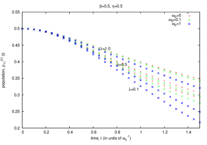
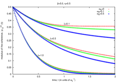
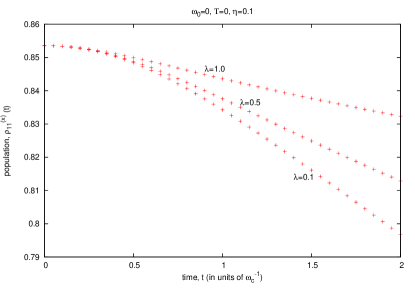
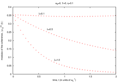
After laying down the methods for obtaining the solutions, we now can observe what they look like in graphs. There are four parameters to be analysed:

  • λ𝜆\lambda, the coupling strength between the system and the measuring apparatus;

  • η,𝜂\eta, the coupling strength between the system and the environment;

  • ω0subscript𝜔0\omega_{0}, the splitting, in frequency units, between the two energy levels of the principal system, henceforth called the natural frequency of the system;

  • T𝑇T, the environment temperature, also expressed in terms of β=1/kBT𝛽1subscript𝑘𝐵𝑇\beta=1/k_{B}T, where kBsubscript𝑘𝐵k_{B} is the Boltzmann constant. Note that T=0𝑇0T=0 corresponds to the limit in which β𝛽\beta\rightarrow\infty.

In this section, we observe how the measurement, represented by λ𝜆\lambda, affects the evolution of the system for different values of the other three parameters η𝜂\eta, ω0subscript𝜔0\omega_{0}, and β𝛽\beta.

It may be noted that in some cases the natural frequency of the system is taken as zero (ω0=0subscript𝜔00\omega_{0}=0). This is not simply a manner of simplifying the calculations, despite certainly having this advantage. This is equivalent to turning off the natural evolution of the two-level system, as in the case of a memory qubit. It is, therefore, a situation of relevance in the context of quantum computation, because quantum memories are necessary to the proper synchronization of the internal processes of a quantum computer Q_MEMORY .

V.1 Phase-damping

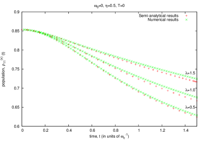
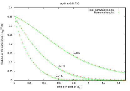
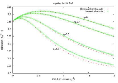
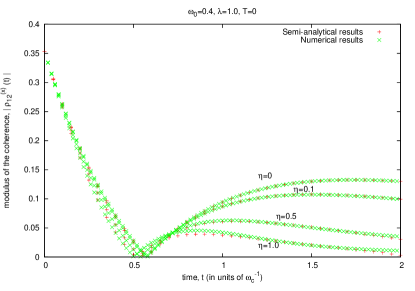
The phase damping channel merely causes the loss of coherence in the basis of σ^zsubscript^𝜎𝑧\hat{\sigma}_{z}, thus having an effect similar to a measurement of this observable. It does not affect the populations in this basis and, therefore, the outcome of the σ^zsubscript^𝜎𝑧\hat{\sigma}_{z} measurement remains unchanged. However, as it makes the coherences disappear, it does affect the outcomes of the measurement of σ^xsubscript^𝜎𝑥\hat{\sigma}_{x}, for example. In this case, as the coherences in the original basis vanish, the populations in the basis of σ^xsubscript^𝜎𝑥\hat{\sigma}_{x} approach 1/2121/2, thus destroying any information that we initially could obtain from a measurement of that observable.

V.1.1 The z-component measurement

Eq. (41) is the complete analytical solution for this case, and it includes all the parameters of our problem. For this case, we can see key-23 that:

  • the populations are constant in time, for any value of the parameters ω0subscript𝜔0\omega_{0}, λ𝜆\lambda, η𝜂\eta, and T𝑇T;

  • the moduli of the coherences are independent of ω0subscript𝜔0\omega_{0} and an increase in the other parameters just makes the decay more intense.

These results are expected, because the frequency ω0subscript𝜔0\omega_{0} only affects the phases of the coherences, and both the measuring apparatus and the environment are responsible for measuring the system in the eigenbasis of σ^zsubscript^𝜎𝑧\hat{\sigma}_{z}, thus causing decoherence. The only new result is that the environmental temperature also helps to increase the decoherence, an effect not unlike those found in other works that did not involve the measuring apparatus key-25 .

V.1.2 The x-component measurement

While in key-23 we had to make the restrictions ω0=0subscript𝜔00\omega_{0}=0 and T=1kBβ=0𝑇1subscript𝑘𝐵𝛽0T=\frac{1}{k_{B}\beta}=0 in (44) to obtain analytical solutions, here the equation is solved numerically to analyse the influence of all parameters.
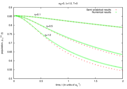
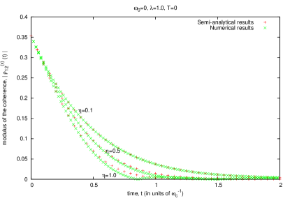
Refer to caption
Refer to caption
Refer to caption
Refer to caption
Figure 1: Populations and coherences in the eigenbasis of the measured observable for ω0=0subscript𝜔00\omega_{0}=0 and T=0𝑇0T=0. In this case the conclusions are the same as those presented in reference key-23 .

Figure 1 reproduces the analytical results of key-23 ; key-24 for ω0=0subscript𝜔00\omega_{0}=0 and T=0𝑇0T=0, namely, that the change in value of the population, caused by the interaction with the environment and therefore increased with η𝜂\eta, is attenuated by the system-apparatus coupling λ𝜆\lambda. Regarding the coherences, which tend to zero in absolute value, we are able to establish a time for the measurement process to reach completion. In key-24 we have found, for this specific situation, an upper limit for the measurement duration:

tM=12λ2lnfsubscript𝑡𝑀12superscript𝜆2𝑓t_{M}=-\frac{1}{2\lambda^{2}}\ln f (58)

where f𝑓f is an arbitrary fraction of the initial value of the modulus of the coherences (0<f<10𝑓10<f<1).

Moreover, the comparison between the solution of the master equation and the numerical results obtained from the superoperator-splitting procedure are in good agreement for low values of η𝜂\eta, but the two graphs depart more and more from each other as the strength of the coupling increases. This is due to the fact that the master equation is a lower-order approximation valid only in the limit of small η𝜂\eta. For higher values of η𝜂\eta, the approximation fails.

After reproducing the numerical results known to the analytical approach, we add a new parameter: the system frequency, ω0subscript𝜔0\omega_{0}. Figure 2 is equivalent to Fig. 1, now considering a non-zero value for ω0subscript𝜔0\omega_{0}.

Refer to caption
Refer to caption
Refer to caption
Refer to caption
Figure 2: Curves referring to the population in the eigenbasis of the measured observable, considering many values of λ𝜆\lambda and η𝜂\eta, and a non-zero value of ω0subscript𝜔0\omega_{0}, while keeping T=0𝑇0T=0.

From Fig. 2, we note that the increase of the system frequency changes the behavior of the populations, which is no longer monotonic. In the time interval considered here, we are able to observe that the populations oscillate. From Fig. 2(c), we observe that, the lower the value of λ𝜆\lambda, the closer is the evolution of the populations to the unperturbed case (dashed lines). This might mislead us into thinking that the finite-time measurement is less efficient than the instantaneous in this case. This notion is false, however, because the state we want to measure is the one at the instant t=0𝑡0t=0, when the measurement apparatus is turned on. In general, the curve with the highest λ𝜆\lambda is still the one that conserves the population closest to its initial value for most of the time, meaning that the measurement protects the system both from the environment and prevents its inherent evolution, as in the Zeno effect.

For the modulus of the coherences, the monotonic behavior is likewise eliminated. However, while for the populations we found a point of maximum, here we find also a point of minimum at zero, where the coherences change sign and their modulus bounces upwards. As the system-environment coupling strength η𝜂\eta becomes more intense, the time when the magnitude of the coherences is zero becomes smaller, while keeping the modulus in general closer to zero even after the point of minimum. A similar effect is observed for λ𝜆\lambda, which is expected from the fact that both the apparatus and the environment interactions are contributing to the decoherence.

Now, we will consider the effects of another parameter neglected in our previous works key-23 ; key-24 : the temperature of the environment. Fig. 3 shows the behavior of populations and coherences for a fixed value of the strength of the coupling between the system and the environment when the system has zero frequency ω0subscript𝜔0\omega_{0}, in the case in which we vary λ𝜆\lambda and T𝑇T. It is possible to observe, for populations, that, while an increase of the temperature makes the deleterious effects of the environment more pronounced, a similar increase in λ𝜆\lambda is capable of compensating for these effects, thus attenuating the rate of population change. Therefore, we can conclude that the simple addition of the environment temperature to the model does not change our previously published conclusions about state protection and measurement error key-23 ; key-24 .
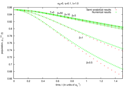
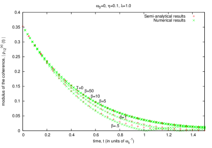
Refer to caption
Refer to caption
Refer to caption
Refer to caption
Figure 3: Curves for the analysis of the effects of the environmental temperature for ω0=0subscript𝜔00\omega_{0}=0.

For the modulus of the coherences, we still have the same effects of faster decrease for higher λ𝜆\lambda, as seen in Fig. 3(d). The only new fact is that the environmental finite temperature has a similar effect to η𝜂\eta in making the coherences approach zero.

Ending the analysis of phase-damping interaction, Fig. 4 shows several curves with fixed and non-zero environment parameters η𝜂\eta and T𝑇T, varying λ𝜆\lambda. As in the previous cases, here we once again verify that the measurement has a twofold effect on the system: it attenuates the changes in the populations and increases the velocity with which the coherences vanish, confirming, so far, the conclusions of our previous works key-23 ; key-24 .
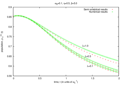
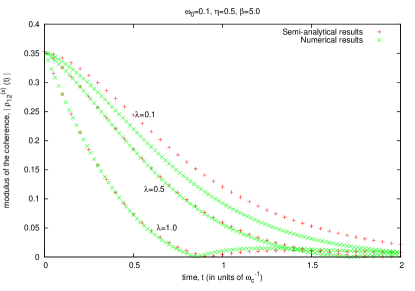
Refer to caption
Refer to caption
Figure 4: Simultaneous influence of the frequency of the system and the environmental temperature.

V.2 Amplitude-damping

The amplitude-damping system-environment interaction differs from phase-damping by not simply being an agent of decoherence. This kind of interaction causes the decay of the excited state |1ket1\left|1\right\rangle to the ground state |2ket2\left|2\right\rangle, thus resulting in the gradual decrease of the population ρ11(t)subscript𝜌11𝑡\rho_{11}\left(t\right) until its complete disappearance.

However, if the temperature is not zero, as in many cases we are treating here, the repopulation of the excited state by the environment will result in a final equilibrium population that lies above zero. This value, proportional to the Boltzmann weight eβω0superscript𝑒Planck-constant-over-2-pi𝛽subscript𝜔0e^{-\hbar\beta\omega_{0}}, increases with temperature (with more energy available, the environment will more easily repopulate the excited state) but decreases with ω0subscript𝜔0\omega_{0} (the higher the energy difference, the more difficult it is to repopulate). For T>0𝑇0T>0 and ω0=0subscript𝜔00\omega_{0}=0, both populations assume a final value of 0.50.50.5, as will be seen below.

V.2.1 The z-component measurement

Contrary to the phase-damping case, amplitude-damping changes the value of the populations in the eigenbasis of σ^zsubscript^𝜎𝑧\hat{\sigma}_{z}, allowing us to observe interesting effects even in this case. Figure 5 shows curves for the population and modulus of the coherence considering several values of η𝜂\eta and λ𝜆\lambda, but still with temperature T𝑇T and frequency ω0subscript𝜔0\omega_{0} turned off.

Refer to caption
Refer to caption
Refer to caption
Refer to caption
Figure 5: Curves for the amplitude-damping interaction, during a measurement of the z𝑧z-component, considering different values of λ𝜆\lambda and η𝜂\eta, but with T=ω0=0𝑇subscript𝜔00T=\omega_{0}=0.

The strengthening of the system-environment coupling η𝜂\eta causes a more intense decrease of the population that can be compensated by an increase in the system-measurement apparatus coupling λ𝜆\lambda. This causes a reduction of the rate of decay analogous to the phase-damping interaction with an x𝑥x-component measurement. For the coherence, the increase of η𝜂\eta or λ𝜆\lambda causes a more intense decrease of the modulus. Therefore, the conclusions from key-23 ; key-24 and the previous section of this article remain valid here, despite our having changed not simply the system-environment interaction but the measured component too.

Let us introduce the system frequency, ω0subscript𝜔0\omega_{0}. From Fig. 6, we note this parameter does not change significantly the population and coherence behavior and, then, we have the same conclusions about the effects of λ𝜆\lambda and η𝜂\eta.

Refer to caption
Refer to caption
Figure 6: Curves for the population and modulus of the coherence considering different values of λ𝜆\lambda, with non-zero ω0subscript𝜔0\omega_{0}.

The coherences have their behavior governed mainly by λ𝜆\lambda, which, as always, makes the modulus go faster to zero while keeping the population closer to its original value. For both variables, a larger system frequency ω0subscript𝜔0\omega_{0} results in a more intense decrease. For the populations, this fact can be easily explained because an increase in the difference between the energy levels makes repopulation more difficult. Then, ω0subscript𝜔0\omega_{0} and λ𝜆\lambda have compensating effects.

With the introduction of the environmental temperature T𝑇T (Fig. 7), we note that, as expected, if we keep T𝑇T constant, we have the well-known protecting effect of the finite-time measurement. On the other hand, the measurement apparatus has its already-observed effect of increasing the reduction rate of the coherences.
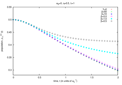
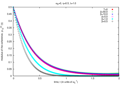
Refer to caption
Refer to caption
Refer to caption
Refer to caption
Figure 7: Introduction of temperature of the environment for the amplitude-damping interaction.

The coherence has its rate of decay sharpened as the environment temperature rises. From the graphs, we can also see that as the environmental temperature rises the population has its decrease rate attenuated, i.e., for a higher temperature, we have a lower measurement error. Hence we see that the environment can have contradictory effects over the measuring process: the coupling intensity η𝜂\eta acts to increase the error associated to the measurement process and decrease the measurement time; however, the temperature T𝑇T acts to reinforce the effects of the system-measurement apparatus coupling λ𝜆\lambda, preventing the decay and increasing the measurement time.

This curious effect is a fortuitous coincidence caused by our choice of ω0subscript𝜔0\omega_{0} and initial state. With ω0=0subscript𝜔00\omega_{0}=0, the thermal energy from the environment will eventually lead to a state of thermal equilibrium between the two systems that will stabilize both populations at the same value. Starting at ρ11(0)=0.5subscript𝜌1100.5\rho_{11}\left(0\right)=0.5, our initial state is already the expected final state. An increase in temperature, in this case, only makes faster the approach of the equilibrium situation.
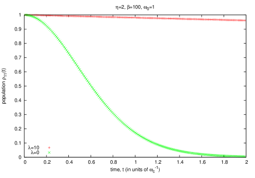
Refer to caption
Figure 8: Attenuated decay caused by the finite-time measurement of the excited state of the system. In green, the curve corresponding to the free evolution of the population; in red, the one indicating its evolution during measurement.

The maintenance of the system in the excited state, however, can be verified even with the ω0subscript𝜔0\omega_{0} and T𝑇T parameters above zero. As illustrated in Fig. 8, we can, with a strong enough choice of the measurement coupling λ𝜆\lambda, keep an ensemble of initially excited systems as close as possible to their original states even at times when they would normally have completely decayed by themselves. This is not simply a more efficient way of performing a measurement of their initial state, but may be a means of observing the quantum Zeno effect key-1 (i. e., keeping a system in its excited state by observing it) for finite-time measurements.

Finally, Fig. 9 shows curves for non-zero environmental temperature, considering constant system-environment coupling and changing the frequency of system and its coupling with the measurement apparatus. We see that the introduction of ω0subscript𝜔0\omega_{0} does not change the evolution of the modulus of the coherences, but intensifies the population decrease for a fixed λ𝜆\lambda.

Refer to caption
Refer to caption
Figure 9: Populations and modulus of the coherences, and their dependence on λ𝜆\lambda and T𝑇T.

Contrary to the case with phase-damping interaction, here we verified some curious effects when we change the system-environment interaction to amplitude-damping:

  • both system-measurement apparatus coupling λ𝜆\lambda and environment temperature T𝑇T can have the effect of preserving the system in the excited state; the first effect is universal, while the second only occurs for certain values of the initial population and temperature, and is a direct consequence of the repopulation of the excited state caused by the thermal energy of the environment;

  • both the system frequency ω0subscript𝜔0\omega_{0} and the system-environment coupling η𝜂\eta intensify the decrease of the population;

  • in general, the conclusions obtained by the measurement of the x𝑥x-component with phase-damping interaction are valid in the present case, except, perhaps, the formula for the upper limit of the measurement duration.

V.2.2 The x-component measurement

Figure 9 shows population and coherence curves for several values of λ𝜆\lambda and η𝜂\eta, while keeping ω0=T=0subscript𝜔0𝑇0\omega_{0}=T=0. As previously observed, the system-environment interaction acts in the sense of accentuating the population decrease and, consequently, the error associated to the measurement process. However, the measurement apparatus still keeps the populations close to their original values.
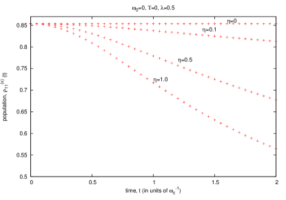
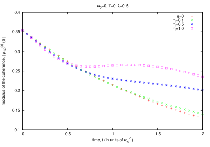
Refer to caption
Refer to caption
Refer to caption
Refer to caption
Figure 10: Populations and coherences for two values of λ𝜆\lambda and different values of η𝜂\eta.

Although we cannot, in this case, obtain a simple expression for the duration of the measurement, we still use the coherences to establish the time at which the system-environment interaction can be interrupted and the reading of the state accomplished - in this case, the time when the coherences assume the constant asymptotic value. Obviously, in more general cases, when the behavior of the system is not simple (the coherences no longer display a monotonic decrease), its physical properties must be considered to the establishment of the measurement time. In these non-monotonous cases, there are at least two possible criteria that could be taken to determine the end of the measurement: the instant when the modulus of the coherences reaches zero, or when it assumes an asymptotically constant value.

The next step is to introduce a system frequency ω0subscript𝜔0\omega_{0}. In this case, we observe a similarity with the behavior of the measurement of the x𝑥x-component for phase-damping interaction: the populations do not exhibit monotonic behavior anymore, instead displaying a maximum point. As the system-environment coupling increases, both its intensity and the time when it occurs decreases. On the other hand, increasing the system-measurement apparatus coupling diminishes the maximum intensity.

Figure 11 shows that the element that determines the qualitative format of the curves is the frequency of the system ω0subscript𝜔0\omega_{0}. One should note, while observing these results, that all of them were plotted in the basis of the measurement, that is, σ^xsubscript^𝜎𝑥\hat{\sigma}_{x}. These populations depend on the real part of the coherences in the basis of σ^zsubscript^𝜎𝑧\hat{\sigma}_{z}, which is expected to oscillate when ω00subscript𝜔00\omega_{0}\neq 0. For example, in the case of a spin in a z𝑧z-oriented field, the expectation values of σ^xsubscript^𝜎𝑥\hat{\sigma}_{x} and σ^ysubscript^𝜎𝑦\hat{\sigma}_{y} change while the spin rotates around the z𝑧z-axis. This explains the non-monotonous behavior of the populations, a phenomenon observed previously in Fig. 2(a).
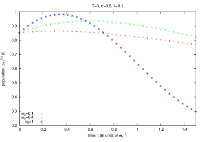
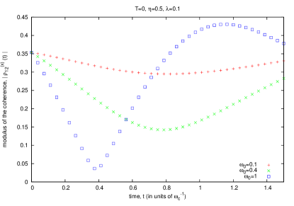
Refer to caption
Refer to caption
Refer to caption
Refer to caption
Figure 11: Populations and coherences obtained for a fixed η𝜂\eta, varying λ𝜆\lambda and ω0subscript𝜔0\omega_{0}.

Lastly, we analyse the effects of the environmental temperature. For the present case, contrary to the previous section, we verified that, for a larger environmental temperature, the rate of change of the populations is increased. Then, the environment - through T𝑇T - acts to increase the measurement error, reinforcing the fact that the temperature-originated protection found in the previous section was merely fortuitous.

Figure 12 shows several curves for different environment temperatures and ω0=0subscript𝜔00\omega_{0}=0 and, after that, curves where all relevant parameters are present. Once again, the qualitative behavior is determined by ω0subscript𝜔0\omega_{0}.

Refer to caption
Refer to caption
Refer to caption
Refer to caption
Refer to caption
Refer to caption
Figure 12: Effect of the introduction of T𝑇T, followed by the introduction of T𝑇T and ω0subscript𝜔0\omega_{0}. The last three graphs contain the coherences corresponding to the populations plotted in the third one. To avoid confusion caused by the superposition of different curves, they were broken in three.

VI Conclusions and Perspectives

In this work, we employed the formalism that we developed to treat the hybrid formulation of the master equation key-20 , which helped us to simplify the analytic solution, although the system of equations encountered still had to be solved numerically. In both cases, phase and amplitude damping, the interaction between the system and the measurement apparatus diminishes the effects of the noise on the population of the main system, allowing us to generalize our previous conclusions in this sense key-23 . This means that in both cases we are capable of performing a measurement more efficiently if instead of measuring it instantly at t>0𝑡0t>0, we perform a finite-time measurement from 00 to t𝑡t, even at finite temperature. Likewise, for finite-time measurements, an increase in the system-apparatus coupling constant λ𝜆\lambda is capable of making their results more reliable.

The possibility of application of this kind of measurement to improve the quality of the results depends, however, on the practical existence of measurements that can be performed for a finite period of time, in accordance to the model. In the following appendix, we propose a verification of our hypothesis by a simple experimental setting that, if yielding positive results, would not only affect fundamental aspects of quantum theory but, also, other areas such as quantum information theory key-26 .

Besides the assumption that measurements are finite in time, we took the additional step of approximating the system-apparatus interaction as a Markovian process. Even though having the advantage of simplifying our calculations, this is a hypothesis far less straightforward to justify than the finite-time measurement. Future prospects of our research include eliminating this approximation by letting the λ2superscript𝜆2\lambda^{2} vary in timeQZE_Turku and seeing the effects of this in the noisy measurement process.

Acknowledgments

C. A. Brasil acknowledges support from Coordenação de Aperfeiçoamento de Pessoal de Nível Superior (CAPES) and Fundação de Amparo à Pesquisa do Estado de São Paulo (FAPESP), project number 2011/19848-4, Brazil, and to A. O. Caldeira for hospitality and useful discussions.

L. A. de Castro acknowledges support from Coordenação de Aperfeiçoamento de Pessoal de Nível Superior (CAPES).

R. d. J. Napolitano acknowledges support from Conselho Nacional de Desenvolvimento Científico e Tecnológico (CNPq), Brazil.

Appendix: Proposed Experimental Test

Beyond what has been shown in key-28 , here we propose an alternative experimental application of our formalism. Throughout this and previous articles, we made the bold assumption that the measurement can ultimately be described as a finite-time interaction between the system and a large number of (traced-out) degrees of freedom of the apparatus. Moreover, we assumed that this interaction could be described as Markovian. The accuracy of these assumptions is far from uncontroversial, but could be verified in the experimental test described below, which is based on the theory of weak measurements. WeakMeasurements We should note, before proceeding, that in this test we are mostly interested in the validity of the first assumption, that is, the possibility of making finite-time measurements in practice. In case the Markovian approximation is not valid the experiment can still be used to test the extension of our model to non-Markovian measurement apparatus, currently a work in progress.

In this experimental setting, we analyse what happens when we measure the magnetic moment of a spin-1/2 particle with two Stern-Gerlach apparatus, which corresponds to the kind of two-state measurement described in the body of this article. The first apparatus performs a “weak” measurement, i. e., one that does not completely destroy the coherences; and the second promoting the full collapse of the wave function. As the second equipment’s task is simply to measure the state of the spins of the particle after they have been through the first equipment, we shall not concern ourselves with its inner workings, and it will not be necessary for this second apparatus to actually be a Stern-Gerlach.

We choose the direction of the z𝑧z axis so the final measurement is done along it. As this experiment will yield trivial results if we choose the observable measured by the weak measurement as the same the second one, we will tilt the first apparatus with an angle β𝛽\beta in respect with the z𝑧z axis. In this case, the observable being measured by it will be:

σ^β=cosβσ^z+sinβσ^x,subscript^𝜎𝛽𝛽subscript^𝜎𝑧𝛽subscript^𝜎𝑥\hat{\sigma}_{\beta}=\cos\beta\hat{\sigma}_{z}+\sin\beta\hat{\sigma}_{x},

where we are calling the direction along which the particles move the y𝑦y axis.

We shall not make any assumptions about the initial state of the spins of the particles, allowing it to be represented by any 2×2222\times 2 density matrix ρ^(0)^𝜌0\hat{\rho}\left(0\right). When these particles cross the first equipment, which we will consider noiseless for simplicity, it will reduce their coherences (in the basis of eigenstates of σ^βsubscript^𝜎𝛽\hat{\sigma}_{\beta}) to a fraction 0<b<10𝑏10<b<1 of their original value, while leaving the populations intact. For “strong”, or “complete” measurements, the wave function collapse would result in the coherences completely vanishing (b=0𝑏0b=0), but for a weak measurement b𝑏b is actually closer to one.

Explicitly, we can write that, if a particle enters the apparatus at t=0𝑡0t=0 and leaves it at τ𝜏\tau, its final state will be:

ρ^(τ)=12[1+b(τ)]ρ^(0)+12[1b(τ)]σ^βρ^(0)σ^β.^𝜌𝜏12delimited-[]1𝑏𝜏^𝜌012delimited-[]1𝑏𝜏subscript^𝜎𝛽^𝜌0subscript^𝜎𝛽\hat{\rho}\left(\tau\right)=\frac{1}{2}\left[1+b\left(\tau\right)\right]\hat{\rho}\left(0\right)+\frac{1}{2}\left[1-b\left(\tau\right)\right]\hat{\sigma}_{\beta}\hat{\rho}\left(0\right)\hat{\sigma}_{\beta}.

In the equation above, we have given the fraction b𝑏b a time dependence, which is precisely the hypothesis we wish to test. If the measurement is instantaneous, this function will be constant, while it will display other kinds of behavior if it is actually a dynamical process. Therefore, our experiment should be capable of providing us information about the form of b(t)𝑏𝑡b\left(t\right).

The final measurement, if performed correctly, will give us simply the expectation value of the variable σ^zsubscript^𝜎𝑧\hat{\sigma}_{z} at t=τ𝑡𝜏t=\tau, regardless of how much time it takes to extract this information from the quantum system, or of how this process is performed. Therefore, from the equation above, we can conclude that the expectancy value of the experiment will be:

σ^z(τ)=[cos2β+b(τ)sin2β]σ^z(0)+12[1b(τ)]sin(2β)σ^x(0),delimited-⟨⟩subscript^𝜎𝑧𝜏delimited-[]superscript2𝛽𝑏𝜏superscript2𝛽delimited-⟨⟩subscript^𝜎𝑧012delimited-[]1𝑏𝜏2𝛽delimited-⟨⟩subscript^𝜎𝑥0\left\langle\hat{\sigma}_{z}\right\rangle\left(\tau\right)=\left[\cos^{2}\beta+b\left(\tau\right)\sin^{2}\beta\right]\left\langle\hat{\sigma}_{z}\right\rangle\left(0\right)+\frac{1}{2}\left[1-b\left(\tau\right)\right]\sin\left(2\beta\right)\left\langle\hat{\sigma}_{x}\right\rangle\left(0\right),

if we consider that the system does not evolve between the two measurements, i. e. ω0=0subscript𝜔00\omega_{0}=0.

Comparing this theoretical formula with the results of the experiments described below, one would be able to deduce the form of the function b(t)𝑏𝑡b\left(t\right). Indeed, the results of σ^z(τ)delimited-⟨⟩subscript^𝜎𝑧𝜏\left\langle\hat{\sigma}_{z}\right\rangle\left(\tau\right) and σ^z(0)delimited-⟨⟩subscript^𝜎𝑧0\left\langle\hat{\sigma}_{z}\right\rangle\left(0\right)can be measured directly by turning on or off the first Stern-Gerlach apparatus. If σ^x(0)delimited-⟨⟩subscript^𝜎𝑥0\left\langle\hat{\sigma}_{x}\right\rangle\left(0\right) cannot be known from the preparation of the spins, we can eliminate it from the equation by taking β=π/2𝛽𝜋2\beta=\pi/2:

σ^z(τ)=b(τ)σ^z(0),β=π2.formulae-sequencedelimited-⟨⟩subscript^𝜎𝑧𝜏𝑏𝜏delimited-⟨⟩subscript^𝜎𝑧0𝛽𝜋2\left\langle\hat{\sigma}_{z}\right\rangle\left(\tau\right)=b\left(\tau\right)\left\langle\hat{\sigma}_{z}\right\rangle\left(0\right),\quad\beta=\frac{\pi}{2}.

This is probably the preferred setting of the experiment, but we will proceed nevertheless treating β𝛽\beta as any angle, to keep our results as general as possible. The only thing we have to keep in mind is that we cannot choose β=nπ𝛽𝑛𝜋\beta=n\pi, n,𝑛n\in\mathbb{Z},as this would reduce the expression above to something trivial.

VI.1 Checking if the measurement is “weak”

The experiment proposed requires the assumption that the first measurement is weak. If it turns out that the first Stern-Gerlach is actually completely collapsing the wave function, there will be no meaningful results.

In this undesirable situation, we would have b=0𝑏0b=0, yielding a measurement of:

σ^zb=0(τ)=cos2βσ^z(0)+12sin(2β)σ^x(0).subscriptdelimited-⟨⟩subscript^𝜎𝑧𝑏0𝜏superscript2𝛽delimited-⟨⟩subscript^𝜎𝑧0122𝛽delimited-⟨⟩subscript^𝜎𝑥0\left\langle\hat{\sigma}_{z}\right\rangle_{b=0}\left(\tau\right)=\cos^{2}\beta\left\langle\hat{\sigma}_{z}\right\rangle\left(0\right)+\frac{1}{2}\sin\left(2\beta\right)\left\langle\hat{\sigma}_{x}\right\rangle\left(0\right).

We should, therefore, make sure our test results are sufficiently distant from those expected when the measurement is not weak. The difference between and the preferred and failed cases is of:

Δz|σ^zb1(τ)σ^zb=0(τ)||cos2βσ^z(0)12sin(2β)σ^x(0)|.subscriptΔ𝑧subscriptdelimited-⟨⟩subscript^𝜎𝑧𝑏1𝜏subscriptdelimited-⟨⟩subscript^𝜎𝑧𝑏0𝜏superscript2𝛽delimited-⟨⟩subscript^𝜎𝑧0122𝛽delimited-⟨⟩subscript^𝜎𝑥0\Delta_{z}\equiv\left|\left\langle\hat{\sigma}_{z}\right\rangle_{b\approx 1}\left(\tau\right)-\left\langle\hat{\sigma}_{z}\right\rangle_{b=0}\left(\tau\right)\right|\approx\left|\cos^{2}\beta\left\langle\hat{\sigma}_{z}\right\rangle\left(0\right)-\frac{1}{2}\sin\left(2\beta\right)\left\langle\hat{\sigma}_{x}\right\rangle\left(0\right)\right|.

Therefore, it is desirable to choose the initial conditions and the angle β𝛽\beta so that ΔzsubscriptΔ𝑧\Delta_{z} is bigger than our experimental errors, in order to distinguish the case when the measurement is weak from the case when it is too strong.

In the best setting, where β=π/2𝛽𝜋2\beta=\pi/2, the undesirable situation has σ^zb=0(τ)=0subscriptdelimited-⟨⟩subscript^𝜎𝑧𝑏0𝜏0\left\langle\hat{\sigma}_{z}\right\rangle_{b=0}\left(\tau\right)=0. This means that, as long as we choose an initial condition satisfying |σ^z(0)|>0delimited-⟨⟩subscript^𝜎𝑧00\left|\left\langle\hat{\sigma}_{z}\right\rangle\left(0\right)\right|>0, we just have to measure an average value distinguishable from zero to be sure we are indeed performing “weak” measurements. The error of the experiment, therefore, must be kept below Δz=|σ^z(0)|>0subscriptΔ𝑧delimited-⟨⟩subscript^𝜎𝑧00\Delta_{z}=\left|\left\langle\hat{\sigma}_{z}\right\rangle\left(0\right)\right|>0. On the other hand, it may also be important to verify if σ^z(τ)delimited-⟨⟩subscript^𝜎𝑧𝜏\left\langle\hat{\sigma}_{z}\right\rangle\left(\tau\right) is distinguishable from σ^z(0)delimited-⟨⟩subscript^𝜎𝑧0\left\langle\hat{\sigma}_{z}\right\rangle\left(0\right), i. e., that some intermediary measurement is being performed.

VI.2 Varying times of measurement

The previous experiment can be only used to make sure that there is a b𝑏b function in action, but gives no information about the time dependency of that function. To acquire information about it, we must vary the measurement periods τ𝜏\tau and see what effect these have in the final result. There are two possible ways of varying the time of exposure in a Stern-Gerlach equipment: you can change the velocity with which the particles cross the apparatus, or you can change the length of their path. It is just important not to change the strength of measurement (by altering the gradient of the magnetic field, for example), instead of the time of exposure of the spin.

In its most general form, the average value measured will be:

σ^z(τ)=A+b(τ)C,delimited-⟨⟩subscript^𝜎𝑧𝜏𝐴𝑏𝜏𝐶\left\langle\hat{\sigma}_{z}\right\rangle\left(\tau\right)=A+b\left(\tau\right)C,

where A𝐴A, C𝐶C are constants. Once we calculate them using the known values of the initial conditions and the tilting of the intermediary measurement β𝛽\beta, we can plot the values of b(τ)𝑏𝜏b\left(\tau\right), thereby verifying whether it is constant or if measurement indeed has a time dependency. For the situation where β=π/2,𝛽𝜋2\beta=\pi/2, the function becomes simply a renormalization of the measured average values:

b(τ)=σ^z(τ)σ^z(0).𝑏𝜏delimited-⟨⟩subscript^𝜎𝑧𝜏delimited-⟨⟩subscript^𝜎𝑧0b\left(\tau\right)=\frac{\left\langle\hat{\sigma}_{z}\right\rangle\left(\tau\right)}{\left\langle\hat{\sigma}_{z}\right\rangle\left(0\right)}.

If the measurement is an instantaneous phenomenon that does not depend on the time of interaction of the apparatus, we should encounter a constant, while a smooth dynamical measurement would produce a positive function with the limits b(τ0)=1𝑏𝜏01b\left(\tau\to 0\right)=1, b(τ)=0𝑏𝜏0b\left(\tau\to\infty\right)=0.

VI.3 Connection with our model of measurement

In our model of measurement as a Markovian interaction between the system and the measurement apparatus, the b(τ)𝑏𝜏b\left(\tau\right) function has the form of a negative exponential:

b(τ)=e2λ2τ,𝑏𝜏superscript𝑒2superscript𝜆2𝜏b\left(\tau\right)=e^{-2\lambda^{2}\tau},

where λ𝜆\lambda is the constant that represents the strength of the coupling between the system and the measurement apparatus. This is a function that satisfies the limits given in the previous section, thus being a plausible candidate for the results that can be found experimentally.

If controlling the time the particles remain under measurement is not a feasible task in some laboratory, one could vary instead the coupling strength with the measurement apparatus (represented by the rate of change of the magnetic field, in the case of the Stern-Gerlach experiment). If the dependence found between b𝑏b and λ2superscript𝜆2\lambda^{2} in this case is exponential, it will not be a confirmation that measurement is a finite-time phenomenon, but it could be a good first step towards confirming our theory. Conversely, if we are capable of controlling τ𝜏\tau and measuring b𝑏b with good precision, we can use the equation above to calculate λ2superscript𝜆2\lambda^{2}, transforming this theoretical parameter into something concrete.

We should note, finally, that the heart of the Markovian approximation is that λ2superscript𝜆2\lambda^{2} is a positive constant. In case it is not, we would still find some change in the value of b(t)𝑏𝑡b\left(t\right), even though not as simple as a negative exponential. Therefore, this experiment could still be used to determine the finite-time length of the measurement, while our model would have to be altered to account for varying of λ2superscript𝜆2\lambda^{2}. As mentioned in the final section of article, these adaptations are currently work in progress.

References

  • (1) M. Jammer, The philosophy of quantum mechanics: the interpretations of quantum mechanics in historical perspective (Wiley, New York, 1974).
  • (2) J. A. Wheeler and W. H. Zurek, Quantum theory and measurement (Princeton University Press, Princeton, 1983).
  • (3) B. L. van der Waerden, Sources of quantum mechanics (North Holland Pub. Co., Amsterdam, 1967).
  • (4) G. S. Im, Archive for History of Exact Sciences 50, 73 (1995).
  • (5) P. A. M. Dirac, Proc. R. Soc. London Sect. A 112, 661 (1926).
  • (6) K. Gottfried, Am. J. Phys. 79, 261 (2011).
  • (7) J. von Neumann, Mathematical foundations of quantum mechanics (Princeton University Press, Princeton, 1953).
  • (8) H. Everett III, Rev. Mod. Phys. 29, 454 (1957).
  • (9) J. A. Wheeler, Rev. Mod. Phys. 29, 463 (1957).
  • (10) B. S. Dewitt and N. Graham, The many-worlds interpretation of quantum mechanics: a fundamental exposition by Hugh Everett, III (Princeton University Press, Princeton, 1973).
  • (11) F. Freitas; O. Freire Jr, Revista Brasileira de Ensino de Física 30, 2307 (2008). (open access)
  • (12) A. Peres, Phys. Rev. A 61, 022116 (2000).
  • (13) G. Lindblad, Commun. Math. Phys. 48, 119 (1976).
  • (14) H.-P. Breuer and F. Petruccione, The theory of open quantum systems (Oxford University Press, Oxford, 2002).
  • (15) C. A. Brasil, F. F. Fanchini, and R. d. J. Napolitano, Revista Brasileira de Ensino de Física 35, 1303 (2013). (open access)
  • (16) I. Percival, Quantum state diffusion (Cambridge University Press, Cambridge, 1998).
  • (17) J. D. Crasser, S. M. Barnett, J. Jeffers and D. T. Pegg, Opt. Commun. 264, 352 (2006).
  • (18) C. A. Brasil and R. d. J. Napolitano, Eur. Phys. J. Plus 126, 91 (2011).
  • (19) S. Nakajima, Prog. Theor. Phys. 20, 948 (1958).
  • (20) R. Zwanzig, J. Chem. Phys. 33, 1338 (1960).
  • (21) L. S. Schulman, Phys. Rev. A 57, 1509 (1998). P. Facchi, and S. Pascazio, Fortschr. Phys. 49, 941 (2001).
  • (22) K. Jacobs, and D. A. Steck, Contemporary Physics 47, 279 (2006).
  • (23) A. Barchielli, L. Lanz, and G. M. Prosperi, Il Nuovo Cimento B 72, 79 (1982). M. Caves, and G. J. Milburn, Phys. Rev. A 36, 5543 (1987).
  • (24) C. A. Brasil, L. A. de Castro, and R. d. J. Napolitano, Phys. Rev. A 84, 022112 (2011).
  • (25) C. A. Brasil, L. A. de Castro, and R. d. J. Napolitano, Found. Phys. 43, 642 (2013).
  • (26) Y. Yan, J. Zou, B.-M. Xu, J.-G. Li and B. Shao, Phys. Rev. A 88, 032320 (2013).
  • (27) H. M. Wiseman and G. J. Milburn, Phys. Rev. Lett. 70, 548 (1993).
  • (28) H. M. Wiseman, Phys. Rev. A 49, 2133 (1994).
  • (29) J. H. Reina, L. Quiroga, and N. F. Johnson, Phys. Rev. A 65, 032326 (2002).
  • (30) B. Misra and E. C. G. Sudarshan, J. Math. Phys. 18, 756 (1977).
  • (31) M. A. Nielsen and I. L. Chuang, Quantum Computation and Quantum Information (Cambridge University Press, Cambridge, 2000).
  • (32) Y. Aharonov, D. Z. Albert, and L. Vaidman, Phys. Rev. Lett. 60, 1351 (1988).
  • (33) A. I. Lvovsky, B. C. Sanders, and W. Tittel, Nature Photon. 3, 706 (2009).
  • (34) J. Piilo et al., Phys. Rev. A. 79, 062112 (2009).