Two-Nucleon Systems in a Finite Volume:
(II) ${}^{3}\hskip-1.8063ptS_{1}$-${}^{3}\hskip-1.8063ptD_{1}$ Coupled Channels and the Deuteron

Abstract

The energy spectra of two nucleons in a cubic volume provide access to the two phase shifts and one mixing angle that define the S-matrix in the ${}^{3}\hskip-1.8063ptS_{1}$-${}^{3}\hskip-1.8063ptD_{1}$ coupled channels containing the deuteron. With the aid of recently derived energy quantization conditions for such systems, and the known scattering parameters, these spectra are predicted for a range of volumes. It is found that extractions of the infinite-volume deuteron binding energy and leading scattering parameters, including the S-D mixing angle at the deuteron pole, are possible from Lattice QCD calculations of two-nucleon systems with boosts of $|\mathbf{P}|\leq\frac{2\pi}{\rm L}\sqrt{3}$ in volumes with $10~{}\rm{fm}\lesssim{\rm L}\lesssim 14~{}\rm{fm}$. The viability of extracting the asymptotic D/S ratio of the deuteron wavefunction from Lattice QCD calculations is discussed.

I Introduction

An overarching goal of modern nuclear physics is to observe and quantify the emergence of low-energy nuclear phenomena from quantum chromodynamics (QCD). A critical step toward this goal is a refinement of the chiral nuclear forces beyond what has been made possible by decades of experimental exploration, using Lattice QCD (LQCD). This numerical technique is making rapid progress toward predicting low-energy nuclear processes with fully-quantified uncertainties Beane et al. (2006); Ishii et al. (2007); Aoki et al. (2008); Beane et al. (2010); Aoki et al. (2010); Beane et al. (2011, 2012, 2012, 2013, 2013); Yamazaki et al. (2012, 2012); Murano et al. (2013). The lightest nucleus, the deuteron, played an important historical role in understanding the form of the nuclear forces and the developments that led to the modern phenomenological nuclear potentials, e.g. Refs. Wiringa et al. (1995); Machleidt (2001). While challenging for LQCD calculations, postdicting the properties of the deuteron, and other light nuclei, is a critical part of the verification of LQCD technology that is required in order to trust predictions of quantities for which there is little or no experimental guidance. In nature, the deuteron, with total angular momentum and parity of $J^{\pi}=1^{+}$, is the only bound state of a neutron and proton, bound by $B_{d}^{\infty}=2.224644(34)~{}{\rm MeV}$. While predominantly S-wave, the non-central components of the nuclear forces (the tensor force) induce a D-wave component, and the $J^{\pi}=1^{+}$ two-nucleon (NN) sector that contains the deuteron is a ${}^{3}\hskip-1.8063ptS_{1}$-${}^{3}\hskip-1.8063ptD_{1}$ coupled-channels system. An important consequence of the nonconservation of orbital angular momentum is that the deuteron is not spherical, and possesses a non-zero quadrupole moment (the experimentally measured value of the electric quadrupole moment of the deuteron is $Q_{d}=0.2859(3)~{}{\rm fm}^{2}$ Bishop and Cheung (1979)). The S-matrix for this coupled-channels system can be parameterized by two phase shifts and one mixing angle, with the mixing angle manifesting itself in the asymptotic $D/S$ ratio of the deuteron wavefunction, $\eta=0.02713(6)$ Biedenharn and Blatt (1954); Mustafa (1993); de Swart et al. (1995). A direct calculation of the three scattering parameters from QCD, at both physical and unphysical light-quark masses, would provide important insights into the tensor components of the nuclear forces.

As LQCD calculations are performed in a finite volume (FV) with certain boundary conditions (BCs) imposed upon the fields, precise determinations of the deuteron properties from LQCD requires understanding FV effects. Corrections to the binding energy of a bound state, such as the deuteron, depend exponentially upon the volume, and are dictated by its size, and also by the range of the nuclear forces. With the assumption of a purely S-wave deuteron, the leading order (LO) volume corrections have been determined for a deuteron at rest in a cubic volume of spatial extent ${\rm L}$ and with the fields subject to periodic BCs in the spatial directions Luscher (1986, 1991); Beane et al. (2004). They are found to scale as ${1\over{\rm L}}e^{-\kappa_{d}^{\infty}{\rm L}}$, where $\kappa_{d}^{\infty}$ is the infinite-volume deuteron binding momentum (in the non-relativistic limit, $\kappa_{d}^{\infty}=\sqrt{MB_{d}^{\infty}}$, with $M$ being the nucleon mass). Volume corrections beyond LO have been determined, and extended to systems that are moving in the volume Koenig et al. (2011); Bour et al. (2011); Davoudi and Savage (2011). As $\eta$, $Q_{d}$, and other observables dictated by the tensor interactions, are small at the physical light-quark masses, FV analyses of existing LQCD calculations Beane et al. (2006, 2013, 2013); Yamazaki et al. (2012) using Lüscher’s method Luscher (1986, 1991) have taken the deuteron to be purely S-wave, neglecting the D-wave admixture, even at unphysical pion masses, introducing a systematic uncertainty into these analyses.  Although the mixing between the S-wave and D-wave is known to be small at the physical light-quark masses, its contribution to the calculated FV binding energies must be determined in order to address this systematic uncertainty. Further, it is not known if the mixing between these channels remains small at unphysical quark masses. As the central and tensor components of the nuclear forces have different forms, their contribution to the FV effects will, in general, differ. The contributions from the tensor interactions are found to be relatively enhanced for certain center of mass (CM) boosts in modest volumes due to the reduced spatial symmetry of the system. Most importantly, extracting the S-D mixing angle at the deuteron binding energy, in addition to the S-wave scattering parameters, requires a complete coupled-channels analysis of the FV spectrum.

Extending the formalism developed for coupled-channel systems Detmold and Savage (2004); He et al. (2005); Liu et al. (2006); Bernard et al. (2008); Lage et al. (2009); Bernard et al. (2011); Ishizuka (2009); Briceno and Davoudi (2012); Hansen and Sharpe (2012); Guo et al. (2013); Li and Liu (2013), the FV formalism describing NN systems with arbitrary CM momenta, spin, angular momentum and isospin has been developed recently, providing expressions for the energy eigenvalues in irreducible representations (irreps) of the FV symmetry groups Briceno et al. . In this work, we utilize this FV formalism to explore how the S-D mixing angle at the deuteron binding energy, along with the binding energy itself, can be optimally extracted from LQCD calculations performed in cubic volumes with fields subject to periodic BCs (PBCs) in the spatial directions. Using the phase shifts and mixing angles generated by phenomenological NN potentials that are fit to NN scattering data NIJ , the expected FV energy spectra in the positive-parity isoscalar channels are determined at the physical pion mass (we assume exact isospin symmetry throughout). It is found that correlation functions of boosted NN systems will play a key role in extracting the S-D mixing angle in future LQCD calculations. The FV energy shifts of the ground state of different irreps of the symmetry groups associated with momenta $\mathbf{P}=\frac{2\pi}{\rm L}(0,0,1)$ and $\frac{2\pi}{\rm L}(1,1,0)$, are found to have enhanced sensitivity to the mixing angle in modest volumes and to depend both on its magnitude and sign. A feature of the FV spectra, with practical implications for future LQCD calculations, is that the contribution to the energy splittings from channels with $J>1$, made possible by the reduced symmetry of the volume, are negligible for ${\rm L}\gtrsim 10~{}\text{fm}$ as the phase shifts in those channels are small at low energies. As the generation of multiple ensembles of gauge-field configurations at the physical light-quark masses will require significant computational resources on capability-computing platforms, we have investigated the viability of precision determinations of the deuteron binding energy and scattering parameters from one lattice volume using the six bound-state energies associated with CM momenta $|\mathbf{P}|\leq\frac{2\pi}{\rm L}\sqrt{3}$. We have also considered extracting the asymptotic D/S ratio from the behavior of the deuteron FV wavefunction and its relation to the S-D mixing angle.

II Deuteron and the Finite Volume Spectrum

The spectra of energy eigenvalues of two nucleons in the isoscalar channel with positive parity in a cubic volume subject to PBCs are dictated by the S-matrix elements in this sector, including those defining the ${}^{3}\hskip-1.8063ptS_{1}$-${}^{3}\hskip-1.8063ptD_{1}$ coupled channels that contain the deuteron. The following determinant condition,

$$\text{det}[\mathcal{M}^{-1}+\delta\mathcal{G}^{V}]=0\ \ \ ,$$ (1)

provides the relation between the infinite volume on-shell scattering amplitude $\mathcal{M}$ and the FV CM energy of the NN system below the inelastic threshold Briceno et al. . In this work, we restrict ourselves to nonrelativistic (NR) quantum mechanics, and as such the energy-momentum relation is ${\rm E}_{NR}={\rm E}-2M={\rm E}_{NR}^{*}+{\rm E}_{CM}=\frac{k^{*2}}{M}+\frac{\mathbf{P}^{2}}{4M}$, where $\mathbf{P}$ is the total momentum of the system, and $\mathbf{k}^{*}$ is the momentum of each nucleon in the CM frame. The subscript will be dropped for the remainder of the paper, simply denoting ${\rm E}_{NR}^{(*)}$ by ${\rm E}^{(*)}$. Due to the PBCs, the total momentum is discretized, $\mathbf{P}=\frac{2\pi}{\rm L}\mathbf{d}$, with $\mathbf{d}$ being an integer triplet that will be referred to as the boost vector. $\delta\mathcal{G}^{V}$ is a matrix in the basis of $\left|JM_{J}(LS)\right\rangle$ where $J$ is the total angular momentum, $M_{J}$ is the eigenvalue of the $\hat{J}_{z}$ operator, and $L$ and $S$ are the orbital angular momentum and the total spin of the channel, respectively. The matrix elements of $\delta\mathcal{G}^{V}$ in the positive-parity isoscalar channel in this basis are,

$$\left[\delta\mathcal{G}^{V}\right]_{JM_{J},LS;J^{\prime}M_{J}^{\prime},L^{\prime}S^{\prime}}=\frac{iMk^{*}}{4\pi}\delta_{S1}\delta_{S^{\prime}1}\left[\delta_{JJ^{\prime}}\delta_{M_{J}M_{J}^{\prime}}\delta_{LL^{\prime}}+i\sum_{l,m}\frac{(4\pi)^{3/2}}{k^{*l+1}}c_{lm}^{\mathbf{d}}(k^{*2};{\rm L})\right.$$

$$\qquad\qquad~{}\left.\times\sum_{M_{L},M_{L}^{\prime},M_{S}}\langle JM_{J}|LM_{L}1M_{S}\rangle\langle L^{\prime}M_{L}^{\prime}1M_{S}|J^{\prime}M_{J}^{\prime}\rangle\int d\Omega~{}Y^{*}_{LM_{L}}Y^{*}_{lm}Y_{L^{\prime}M_{L}^{\prime}}\right]\ \ ,$$ (2)

and are evaluated at the on-shell momentum of each nucleon in the CM frame, $k^{*}=\sqrt{M{\rm E}^{*}-{|\mathbf{P}|^{2}}/{4}}$. $\langle JM_{J}|LM_{L}1M_{S}\rangle$ and $\langle L^{\prime}M_{L}^{\prime}1M_{S}|J^{\prime}M_{J}^{\prime}\rangle$ are Clebsch-Gordan coefficients, and $c_{lm}^{\mathbf{d}}(k^{*2};{\rm L})$ is a kinematic function related to the three-dimensional zeta function, $\mathcal{Z}^{\mathbf{d}}_{lm}$, Luscher (1986, 1991); Rummukainen and Gottlieb (1995); Christ et al. (2005); Kim et al. (2005),

$$\hskip 28.45274ptc^{\mathbf{d}}_{lm}(k^{*2};{\rm L}) = \frac{\sqrt{4\pi}}{\rm L^{3}}\left(\frac{2\pi}{\rm L}\right)^{l-2}\mathcal{Z}^{\mathbf{d}}_{lm}[1;(k^{*}{\rm L}/2\pi)^{2}]\ \ \ ,$$

$$\mathcal{Z}^{\mathbf{d}}_{lm}[s;x^{2}] = \sum_{\mathbf{n}}\frac{|\mathbf{r}|^{l}Y_{l,m}(\mathbf{r})}{(r^{2}-x^{2})^{s}}\ \ \ ,$$ (3)

where $\mathbf{\mathbf{r}}=\mathbf{n}-\mathbf{d}/2$ with $\mathbf{n}$ an integer triplet.

The finite-volume matrix $\delta\mathcal{G}^{V}$ is neither diagonal in the $J$ basis nor in the $LS$ basis, as is clear from the form of Eq. (2). As a result of the scattering amplitudes in higher partial waves being suppressed at low-energies, the infinite-dimensional matrices present in the determinant condition can be truncated to a finite number of partial waves. For the following analysis of positive-parity isoscalar channel, the scattering in all but the S- and D-waves are neglected. With this truncation, the scattering amplitude matrix $\mathcal{M}$ can be written as

$${\mathcal{M}}=\left(\begin{array}[]{cccc}\mathcal{M}_{1,S}&\mathcal{M}_{1,SD}&0&0\\ \mathcal{M}_{1,SD}&\mathcal{M}_{1,D}&0&0\\ 0&0&\mathcal{M}_{2,D}&0\\ 0&0&0&\mathcal{M}_{3,D}\\ \end{array}\right)\ \ \ ,$$ (8)

where the first subscript of the diagonal elements, $\mathcal{M}_{J,L}$, denotes the total angular momentum of the channel and the second subscript denotes the orbital angular momentum. The off-diagonal elements in $J=1$ sub-block are due to the S-D mixing. In the $J=3$ channel, there is a mixing between $L=2$ and $L=4$ partial waves, but as scattering in the $L=4$ partial wave is being neglected, the scattering amplitude in this channel remains diagonal. Each element of this matrix is a diagonal matrix of dimension $(2J+1)\times(2J+1)$ dictated by the $M_{J}$ quantum number.

$\hskip 8.5359pt\mathbf{d}\hskip 8.5359pt$	point group	classification	$\hskip 8.5359ptN_{\text{elements}}\hskip 8.5359pt$	irreps (dimension)
$~{}(0,0,0)~{}$	${O}$	cubic	$24$	$~{}\mathbb{A}_{1}(1),\mathbb{A}_{2}(1),\mathbb{E}(2),\mathbb{T}_{1}(3),\mathbb{T}_{2}(3)~{}$
$~{}(0,0,1)~{}$	$D_{4}$	tetragonal	$8$	$~{}\mathbb{A}_{1}(1),\mathbb{A}_{2}(1),\mathbb{E}(2),\mathbb{B}_{1}(1),\mathbb{B}_{2}(1)~{}$
$~{}(1,1,0)~{}$	$D_{2}$	orthorhombic	$4$	$~{}\mathbb{A}(1),\mathbb{B}_{1}(1),\mathbb{B}_{2}(1),\mathbb{B}_{3}(1)~{}$
$~{}(1,1,1)~{}$	$D_{3}$	trigonal	$6$	$~{}\mathbb{A}_{1}(1),\mathbb{A}_{2}(1),\mathbb{E}(2)~{}$

Table 1: Classification of the point groups corresponding to the symmetry of the FV calculations with boost vectors, $\mathbf{d}$. The forth column shows the number of elements of each group, and the last column gives the irreducible representations of each point group along with their dimensions.

With the aid of the symmetry properties of the FV calculation with different boosts, the determinant condition providing the energy eigenvalues given in Eq. (1) can be decomposed into separate eigenvalue equations corresponding to different irreps of the point group,

$$\det\left[\mathcal{M}^{-1}+\delta\mathcal{G}^{V}\right]\ =\ \prod_{\Gamma^{i}}\det\left[(\mathcal{M}^{-1})_{\Gamma^{i}}+\delta\mathcal{G}^{V}_{\Gamma^{i}}\right]^{N(\Gamma^{i})}\ =\ 0\ \ ,$$ (9)

where $\Gamma^{i}$ labels different irreps of the corresponding point group, and $N({\Gamma^{i}})$ denotes the dimensionality of each irrep. Table 1 summarizes some characteristics of the cubic ($O$), tetragonal ($D_{4}$), orthorhombic ($D_{2}$) and trigonal ($D_{3}$) point groups that correspond to systems with boosts $\mathbf{d}=0$, $(0,0,1)$, $(1,1,0)$ and $(1,1,1)$, respectively. Such a reduction has been carried out in Ref. Briceno et al. for all possible NN channels with boosts $|\mathbf{d}|\leq\sqrt{2}$. For the boosts considered in Ref. Briceno et al. , as well as for $\mathbf{d}=(1,1,1)$, the necessary QCs for the NN system in the positive-parity isoscalar channel are given in Appendix A. It is worth noting that for systems composed of equal-mass NR particles, these QCs can be also utilized for boosts of the form $(2n_{1},2n_{2},2n_{3})$, $(2n_{1},2n_{2},2n_{3}+1)$, $(2n_{1}+1,2n_{2}+1,2n_{3})$ and $(2n_{1}+1,2n_{2}+1,2n_{3}+1)$ where $n_{1},n_{2},n_{3}$ are integers, and all cubic rotations of these vectors Briceno et al. .

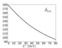
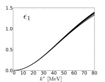
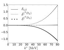
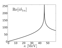
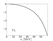
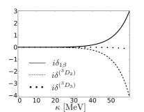
Figure 1: Fits to the experimental values of (a) the $\alpha$-wave phase shift, (b) the mixing angle and (c) the $J=1$ $\beta$-wave and $J=2,3$ D-wave phase shifts (in degrees), in the Blatt-Biedenharn (BB) parameterization Blatt and Biedenharn (1952), as a function of momentum of each nucleon in the CM frame, $k^{*}$, based on six different phase shifts analyses Stoks et al. (1993, 1994); Rijken and Stoks (1996, 1996). (d) The $\alpha$-wave phase shift, (e) the mixing angle and (f) the $J=1$ $\beta$-wave and $J=2,3$ D-wave phase shifts (in degrees) as a function of $\kappa=-ik^{*}$ obtained from the fit functions.

Although the ultimate goal is to utilize the QCs in the analysis of the NN spectra extracted from LQCD calculations, they can be used, in combination with the experimental NN scattering data, to predict the FV spectra at the physical light-quark masses, providing important guidance for future LQCD calculations. While for scattering states, the phase shifts and mixing angle from phenomenological analyses of the experimental data Stoks et al. (1993, 1994); Rijken and Stoks (1996, 1996) can be used in the QCs, for bound states, however, it is necessary to use fit functions of the correct form to be continued to negative energies. The Blatt-Biedenharn (BB) parameterization Blatt and Biedenharn (1952); Biedenharn and Blatt (1954) is chosen for the $J=1$ S-matrix,

$$S_{(J=1)}=\left(\begin{array}[]{cc}\cos\epsilon_{1}&-\sin\epsilon_{1}\\ \sin\epsilon_{1}&\cos\epsilon_{1}\\ \end{array}\right)\left(\begin{array}[]{cc}e^{2i\delta_{1\alpha}}&0\\ 0&e^{2i\delta_{1\beta}}\\ \end{array}\right)\left(\begin{array}[]{cc}\cos\epsilon_{1}&\sin\epsilon_{1}\\ -\sin\epsilon_{1}&\cos\epsilon_{1}\\ \end{array}\right),$$ (16)

whose mixing angle, $\epsilon_{1}$, when evaluated at the deuteron binding energy, is directly related to the asymptotic D/S ratio in the deuteron wavefunction. $\delta_{1\alpha}$ and $\delta_{1\beta}$ are the scattering phase shifts corresponding to two eigenstates of the S-matrix; the so called “$\alpha$” and “$\beta$” waves respectively. At low energies, the $\alpha$-wave is predominantly S-wave with a small admixture of the D-wave, while the $\beta$-wave is predominantly D-wave with a small admixture of the S-wave. The location of the deuteron pole is determined by one condition on the $\alpha$-wave phase shift, $\cot\delta_{1\alpha}|_{k^{*}=i\kappa}=i$. In addition, $\epsilon_{1}$ in this parameterization is an analytic function of energy near the deuteron pole (in contrast with $\bar{\epsilon}$ in the barred parameterization Stapp et al. (1957)). With a truncation of $l_{max}=2$ imposed upon the scattering amplitude matrix in Eq. (1), the scattering parameters required for the analysis of the FV spectra are $\delta_{1\alpha}$, $\delta_{1\beta}$, $\delta^{(^{3}D_{2})}$, $\delta^{(^{3}D_{3})}$ and $\epsilon_{1}$. Fits to six different phase-shift analyses (PWA93 Stoks et al. (1993), Nijm93 Stoks et al. (1994), Nijm1 Stoks et al. (1994), Nijm2 Stoks et al. (1994), Reid93 Stoks et al. (1994) and ESC96 Rijken and Stoks (1996, 1996)) obtained from Ref. NIJ are shown in Fig. 1(a-c).  In order to obtain the scattering parameters at negative energies, the fit functions are continued to imaginary momenta, $k^{*}\rightarrow i\kappa$. Fig. 1(d-f) shows the phase shifts and the mixing angle as a function of $\kappa$ below the t-channel cut (which approximately corresponds to the positive-energy fitting range). $\epsilon_{1}$ is observed to be positive for positive energies, and becomes negative when continued to negative energies (see Fig. 1). The slight difference between phenomenological models gives rise to a small “uncertainty band” for each of the parameters.

J	$O$	${D}_{4}$	${D}_{2}$	${D}_{3}$
1	$\mathbb{T}_{1}:(\mathcal{Y}_{11},\mathcal{Y}_{10},\mathcal{Y}_{1-1})$	$\mathbb{A}_{2}:\mathcal{Y}_{10}$	$\mathbb{B}_{1}:\mathcal{Y}_{10}$	$\mathbb{A}_{2}:\mathcal{Y}_{10}$
		$\mathbb{E}:\left(\overline{\mathcal{Y}}_{11},\widetilde{\mathcal{Y}}_{11}\right)$	$\mathbb{B}_{2}:\overline{\mathcal{Y}}_{11},~{}\mathbb{B}_{3}:\widetilde{\mathcal{Y}}_{11}$	$\mathbb{E}:\left(\overline{\mathcal{Y}}_{11},\widetilde{\mathcal{Y}}_{11}\right)$

Table 2: Decomposition of the $J=1$ irrep of the rotational group in terms of the irreps of the cubic ($O$), tetragonal ($D_{4}$), orthorhombic ($D_{2}$) and trigonal ($D_{3}$) groups, see Refs. Luscher (1991); Feng et al. (2004); Dresselhaus et al. (2008). The corresponding basis functions of each irrep are also shown in terms of the SO(3) functions $\mathcal{Y}_{lm}$, where $\overline{\mathcal{Y}}_{lm}\equiv\mathcal{Y}_{lm}+\mathcal{Y}_{l-m}$ and $\widetilde{\mathcal{Y}}_{lm}\equiv\mathcal{Y}_{lm}-\mathcal{Y}_{l-m}$.

For the NN system at rest in the positive-parity isoscalar channel, the only irrep of the cubic group that has overlap with the $J=1$ sector is $\mathbb{T}_{1}$, see Table 2, which also has overlap with the J=3 and higher channels. Using the scattering parameters of the $J=1$ and $J=3$ channels, the nine lowest $\mathbb{T}_{1}$ energy levels (including the bound-state level) are shown in Fig. 2 as a function of ${\rm L}$. In the limit that $\epsilon_{1}$ vanishes, the $\mathbb{T}_{1}$ QC, given in Eq. (42), can be written as a product of two independent QCs. One of these QCs depends only on $\delta_{1\alpha}\rightarrow\delta^{(^{3}S_{1})}$, while the other depends on $\delta_{1\beta}\rightarrow\delta^{(^{3}D_{1})}$ and $\delta^{(^{3}D_{3})}$. By comparing the $\mathbb{T}_{1}$ spectrum with that obtained for $\epsilon_{1}=0$, the $\mathbb{T}_{1}$ states can be classified as predominantly S-wave or predominantly D-wave states. The dimensionless quantity $\tilde{k}^{2}=ME^{*}{\rm{L}}^{2}/4\pi^{2}$ is shown as a function of volume in Fig. 2, from which it is clear that the predominantly D-wave energy levels remain close to the non-interacting energies, corresponding to $\tilde{k}^{2}=1,2,3,4,5,6,8,\ldots$, consistent with the fact that both the mixing angle and the D-wave phase shifts are small at low energies, as seen in Fig. 1. The states that are predominantly S-wave are negatively shifted in energy compared with the non-interacting states due to the attraction of the NN interactions.

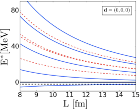
Figure 2: (a) The nine lowest energy eigenvalues satisfying the QC for the $\mathbb{T}_{1}$-irrep of the cubic group, Eq. (42), and (b) the dimensionless quantity $\tilde{k}^{2}=ME^{*}{\rm{L}}^{2}/4\pi^{2}$ as a function of ${\rm L}$. The blue-solid lines correspond to states that are predominantly S-wave, while the red-dashed lines represent states that are predominantly D-wave. The black-dashed line shows the infinite-volume binding energy of the deuteron.

Focusing on the deuteron, it is important to quantify the effect of the mixing between the S-wave and D-wave on the energy of the deuteron in the FV. The upper panel of Fig. 3 provides a closer look at the binding energy of the deuteron as function of ${\rm L}$ extracted from the $\mathbb{T}_{1}$ QC given in Eq. (42). While in larger volumes the uncertainties in the predictions due to the fits to experimental data are a few keV, in smaller volumes the uncertainties increase because the fit functions are valid only below the t-channel cut and are not expected to describe the data above the cut. It is interesting to examine the difference between the bound-state energy obtained from the full $\mathbb{T}_{1}$ QC and that obtained with $\epsilon_{1}=0$, $\delta{\rm E}^{*(\mathbb{T}_{1})}={\rm E}^{*(\mathbb{T}_{1})}-{\rm E}^{*(\mathbb{T}_{1})}(\epsilon_{1}=0)$. This quantity, shown in the lower panel of Fig. 3, does not exceed a few $\rm{keV}$ in smaller volumes, ${\rm L}\lesssim 9~{}\rm{fm}$, and is significantly smaller in larger volumes, demonstrating that the spectrum of $\mathbb{T}_{1}$ irrep is quite insensitive to the small mixing angle in the ${}^{3}\hskip-1.8063ptS_{1}$-${}^{3}\hskip-1.8063ptD_{1}$ coupled channels. Therefore, a determination of the mixing angle from the spectrum of two nucleons at rest will be challenging for LQCD calculations. The spectra in the $\mathbb{A}_{2}/\mathbb{E}$ irreps of the trigonal group for $\mathbf{d}=(1,1,1)$ exhibit the same feature, as shown in Fig. 3. By investigating the QCs in Eqs. (42, 154, 168), it is straightforward to show that the difference between the bound-state energy extracted from the full QCs (including physical and FV-induced mixing between S-waves and D-waves) and from the uncoupled QC is proportional to ${\sin^{2}\epsilon_{1}}$, and is further suppressed by FV corrections and the small $\beta$-wave and D-wave phase shifts.

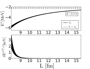
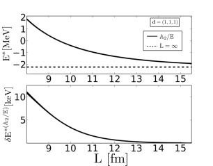
Figure 3: (a) The upper panel shows the energy of two nucleons at rest in the positive-parity isoscalar channel as a function of ${\rm L}$ extracted from the $\mathbb{T}_{1}$ QC given in Eq. (42). The uncertainty band is associated with fits to different phenomenological analyses of the experimental data, and the dashed line denotes the infinite-volume deuteron binding energy. The lower panel shows the contribution of the mixing angle to the energy, $\delta{\rm E}^{*(\mathbb{T}_{1})}={\rm E}^{*(\mathbb{T}_{1})}-{\rm E}^{*(\mathbb{T}_{1})}(\epsilon_{1}=0)$. (b) The same quantities as in (a) for the NN system with ${\bf d}=(1,1,1)$ obtained from the $\mathbb{A}_{2}/\mathbb{E}$ QCs, Eqs. (154, 168).

The boost vectors $\mathbf{d}=(0,0,1)$ and $(1,1,0)$ distinguish the $z$-axis from the other two axes, and result in an asymmetric volume as viewed in the rest frame of the deuteron. In terms of the periodic images of the deuteron, images that are located in the $z$-direction with opposite signs compared with the images in the $x$- and $y$-directions Bour et al. (2011); Davoudi and Savage (2011) result in the quadrupole-type shape modifications to the deuteron, as will be elaborated on in Sec. IV. As a result, the energy of the deuteron, as well as its shape-related quantities such as its quadrupole moment, will be affected more by the finite extent of the volume (compared with the systems with $\mathbf{d}=(0,0,0)$ and $(1,1,1)$).

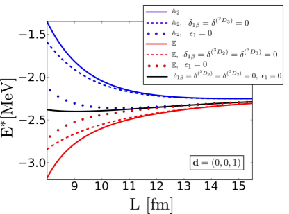
Figure 4: The energy of two nucleons in the positive-parity isoscalar channel with $\mathbf{d}=(0,0,1)$ as a function of ${\rm L}$, extracted from the $\mathbb{A}_{2}$ (red) and $\mathbb{E}$ (blue) QCs given in Eq. (53) and Eqs. (76), respectively. The systematic uncertainties associated with fitting different phenomenological analyses of the experimental data are included.

As is clear from the QCs for $\mathbf{d}=(0,0,1)$ systems, given in Eqs. (53, 76), there are two irreps of the tetragonal group, $\mathbb{A}_{2}$ and $\mathbb{E}$, that have overlap with the $J=1$ channel. These irreps represent states with $M_{J}=0$ for the $\mathbb{A}_{2}$ irrep and $M_{J}=\pm 1$ for the $\mathbb{E}$ irreps, see Table 2. The bound-state energies of these two irreps are shown in Fig. 4 as a function of ${\rm L}$. For comparison, the energy of the bound state with ${\bf d}=(0,0,1)$ in the limit of vanishing mixing angle and D-wave phase shifts is also shown (black-solid curve) in Fig. 4. The energy of the bound states obtained in both the $\mathbb{A}_{2}$ irrep (blue-solid curve) and the $\mathbb{E}$ irrep (red-solid curve) deviate substantially from the energy of the purely S-wave bound state for modest volumes, ${\rm L}\lesssim 14~{}\rm{fm}$.  These deviations are such that the energy gap between the systems in the two irreps is $\sim 80\%$ of the infinite-volume deuteron binding energy at ${\rm L}=8~{}\rm{fm}$, decreasing to $\sim 5\%$ for ${\rm L}=14~{}\rm{fm}$. This gap is largely due to the mixing between S-wave and D-wave in the infinite volume, as verified by evaluating the bound-state energy in the $\mathbb{A}_{2}$ and $\mathbb{E}$ irrep in the limit where $\epsilon_{1}=0$ (the blue and red dotted curves in Fig. 4, respectively.) Another feature of the $\textbf{d}=(0,0,1)$ FV bound-state energy is that the contribution from the $\beta$-wave and D-wave states cannot be neglected for ${\rm L}\lesssim 10~{}\rm{fm}$. The blue (red) dashed curve in Fig. 4 results from the $\mathbb{A}_{2}$ ($\mathbb{E}$) QC in this limit. The D-wave states in the $J=2$ and $J=3$ channels mix with the $J=1$ $\alpha$- and $\beta$-waves due to the reduced symmetry of the system, and as a result they, and the $\beta$-wave state, contribute to the energy of the predominantly S-wave bound state in the FV.

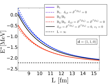
Figure 5: The energy of two nucleons in the positive-parity isoscalar channel with $\mathbf{d}=(1,1,0)$ as a function of ${\rm L}$, extracted from the $\mathbb{B}_{1}$ (red) and $\mathbb{B}_{2}/\mathbb{B}_{3}$ (blue) QCs given in Eqs. (99) and (122, 145), respectively. The systematic uncertainties associated with fitting to different phenomenological analyses of the experimental data are included.

The FV energy eigenvalues for the NN system in the positive-parity isoscalar channel with ${\bf d}=(1,1,0)$ can be obtained from QCs in Eqs. (99) and (122, 145), corresponding to $\mathbb{B}_{1}$ and $\mathbb{B}_{2}/\mathbb{B}_{3}$ irreps of the orthorhombic group, respectively. These irreps represent states with $M_{J}=0$ for the $\mathbb{B}_{1}$ irrep and $M_{J}=\pm 1$ for the $\mathbb{B}_{2}/\mathbb{B}_{3}$ irreps, see Table 2. The bound-state energies of these systems are shown in Fig. 5, and are found to deviate noticeably from the purely S-wave limit (black-solid curve in Fig. 5), however the deviation is not as large as the case of ${\bf d}=(0,0,1)$. The energy gap between the systems in the two irreps is $\sim 30\%$ of the infinite-volume deuteron binding energy at ${\rm L}=8~{}\rm{fm}$, decreasing to $\sim 5\%$ for ${\rm L}=14~{}\rm{fm}$. Eliminating the $\beta$-wave and $J=2,3$ D-wave interactions, leads to the dashed curves in Fig. 5, indicating the negligible effect that they have on the bound-state energy in these irreps.

To understand the large FV energy shifts from the purely $\alpha$-wave estimates for ${\bf d}=(0,0,1)$ and $(1,1,0)$ systems compared with $(0,0,0)$ and $(1,1,1)$ systems, it is instructive to examine the QCs given in Appendix A in the limit where the $\beta$-wave and D-wave phase shifts vanish. This is a reasonable approximation for volumes with ${\rm L}\gtrsim 10~{}\rm{fm}$, as illustrated in Fig. 4 and Fig.  5. It is straightforward to show that in this limit, the QC of the system with $\mathbf{d}=(0,0,0)$ reduces to a purely $\alpha$-wave condition

$$\mathbb{T}_{1} : \hskip 2.84544ptk^{*}\cot\delta_{1\alpha}-4\pi c_{00}^{(0,0,0)}(k^{*2};{\rm L})=0\ \ \ .$$ (17)

The QCs for a system with $\mathbf{d}=(0,0,1)$ are

$$\mathbb{A}_{2}:\hskip 2.84544pt k^{*}\cot\delta_{1\alpha}-4\pi c_{00}^{(0,0,1)}(k^{*2};{\rm L})\ =\ -{1\over\sqrt{5}}\frac{4\pi}{k^{*2}}\ c_{20}^{(0,0,1)}(k^{*2};{\rm L})\ (\sqrt{2}\sin 2\epsilon_{1}-\sin^{2}\epsilon_{1})\ \ ,$$ (18)

$$\mathbb{E}:\hskip 2.84544pt k^{*}\cot\delta_{1\alpha}-4\pi c_{00}^{(0,0,1)}(k^{*2};{\rm L})\ =\ +{1\over 2\sqrt{5}}\frac{4\pi}{k^{*2}}\ c_{20}^{(0,0,1)}(k^{*2};{\rm L})\ (\sqrt{2}\sin 2\epsilon_{1}-\sin^{2}\epsilon_{1})\ \ ,$$ (19)

which includes corrections to the $\alpha$-wave limit that scale with $\sin\epsilon_{1}$ at LO. This is the origin of the large deviations of these energy eigenvalues from the purely S-wave values. The same feature is seen in the systems with $\mathbf{d}=(1,1,0)$, where the QCs reduce to

$$\mathbb{B}_{1}:\hskip 2.84544pt k^{*}\cot\delta_{1\alpha}-4\pi c_{00}^{(1,1,0)}(k^{*2};{\rm L})\ =\ -{1\over\sqrt{5}}\frac{4\pi}{k^{*2}}\ c_{20}^{(1,1,0)}(k^{*2};{\rm L})\ (\sqrt{2}\sin 2\epsilon_{1}-\sin^{2}\epsilon_{1})\ \ \ ,$$ (20)

$$\mathbb{B}_{2}/\mathbb{B}_{3}:\hskip 2.84544pt k^{*}\cot\delta_{1\alpha}-4\pi c_{00}^{(1,1,0)}(k^{*2};{\rm L})\ =\ +{1\over 2\sqrt{5}}\frac{4\pi}{k^{*2}}\ c_{20}^{(1,1,0)}(k^{*2};{\rm L})\ (\sqrt{2}\sin 2\epsilon_{1}-\sin^{2}\epsilon_{1})\ \ \ .$$ (21)

Similarly, the QC with $\mathbf{d}=(1,1,1)$ in this limit is

$$\mathbb{A}_{2}/\mathbb{E} : \hskip 2.84544ptk^{*}\cot\delta_{1\alpha}-4\pi c_{00}^{(1,1,1)}(k^{*2};{\rm L})=0\ \ \ .$$ (22)

The LO corrections to the QCs in Eqs. (17-22) are not only suppressed by the $J=1$ $\beta$-wave and $J=2,3$ D-wave phase shifts, but also by FV corrections that are further exponentially suppressed compared with the leading FV corrections. It is straightforward to show that the leading neglected terms in the QCs presented above are $\sim\frac{1}{\rm L}e^{-2\kappa{\rm L}}\tan{\delta_{1\beta}}$ and $\frac{1}{\rm L}e^{-2\kappa{\rm L}}\tan{\delta_{D_{J=2,3}}}$, while the FV contributions to the approximate relations given in Eqs. (17-22) are $\sim{1\over{\rm L}}e^{-\kappa{\rm L}}$. In Appendix B, the explicit volume dependence of $c^{\mathbf{d}}_{LM}$ functions are given for the case of $k^{*2}=-\kappa^{2}<0$. These explicit forms are useful in obtaining the leading exponential corrections to the QCs. We emphasize that the smaller volumes considered have $\kappa{\rm L}=2-2.5$, and therefore it is not a good approximation to replace the $c^{\mathbf{d}}_{LM}$ functions with their leading exponential terms, and the complete form of these functions should be used in analyzing the FV spectra.

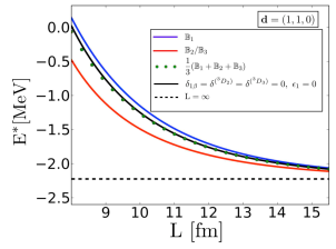
Figure 6: (a) The dotted curve shows the $M_{J}$-averaged quantity $\frac{1}{3}(E^{*(\mathbb{A}_{2})}+2E^{*(\mathbb{E})})$ as function of ${\rm L}$, while the solid curves show the energy of the state in the $\mathbb{A}_{2}$ (blue) and $\mathbb{E}$ (red) irreps of the tetragonal group, as well as that of the state with $\epsilon_{1}=0$ (black). (b) The dotted curve shows the $M_{J}$-averaged quantity $\frac{1}{3}(E^{*(\mathbb{B}_{1})}+E^{*(\mathbb{B}_{2})}+E^{*(\mathbb{B}_{3})})$ as function of ${\rm L}$, while the solid curves show the energy of the state in the $\mathbb{B}_{1}$ (blue) and $\mathbb{B}_{2}/\mathbb{B}_{3}$ (red) irreps of the orthorhombic group, as well as that of the state with $\epsilon_{1}=0$ (black).

In the limit of vanishing $J=1$ $\beta$-wave and $J=2,3$ D-wave phase shifts, the QCs show that the energy shift of each pair of irreps of the systems with $\mathbf{d}=(0,0,1)$ and $(1,1,0)$ differ in sign. It is also the case that the $M_{J}$-averaged energies are approximately the same as the purely S-wave case. In fact, as illustrated in Fig. 6, the energy level corresponding to $\frac{1}{3}(E^{*(\mathbb{A}_{2})}+2E^{*(\mathbb{E})})$ quickly converges to the S-wave energy with ${\bf d}=(0,0,1)$. Similarly, the $M_{J}$-averaged quantity $\frac{1}{3}(E^{*(\mathbb{B}_{1})}+E^{*(\mathbb{B}_{2})}+E^{*(\mathbb{B}_{3})})$ almost coincides with the S-wave state with ${\bf d}=(1,1,0)$, Fig. 6. This is to be expected, as $M_{J}$-averaging is equivalent to averaging over the orientations of the image systems, suppressing the anisotropy induced by the boost phases in the FV corrections, Eqs. (169)-(171). These expressions also demonstrate that, unlike the case of degenerate, scalar coupled-channels systems Berkowitz et al. (2012); Oset (2013), the NN spectra (with spin degrees of freedom) depend on the sign of $\epsilon_{1}$. Of course, this sensitivity to the sign of $\epsilon_{1}$ can be deduced from the full QCs in Eqs. (42-168). Upon fixing the phase convention of the angular momentum states, both the magnitude and sign of the mixing angle can be extracted from FV calculations, as will be discussed in more detail in Section III.

III Extracting the Scattering Parameters From Synthetic Data

Given the features of the energy spectra associated with different boosts, it is interesting to consider how well the scattering parameters can be extracted from future LQCD calculations at the physical pion mass. With the truncations we have imposed, the full QCs for the FV states that have overlap with the ${}^{3}\hskip-1.8063ptS_{1}$-${}^{3}\hskip-1.8063ptD_{1}$ coupled channels depend on four scattering phase shifts and the $J=1$ mixing angle. As discussed in Sec. II, for bound states these are equivalent to QCs that depend solely on $\delta_{1\alpha}$ and $\epsilon_{1}$ up to corrections of $\sim\frac{1}{\rm L}e^{-2\kappa{\rm L}}\tan{\delta_{1\beta}}$ and $\frac{1}{\rm L}e^{-2\kappa{\rm L}}\tan{\delta_{D_{J=2,3}}}$, as given in Eqs. (17-22). By considering the boosts with $|\textbf{d}|\leq\sqrt{3}$, six independent bound-state energies that asymptote to the physical deuteron energy can be obtained. For a single volume, these give six different constraints on $\delta_{1\alpha}$ and $\epsilon_{1}$ for energies in the vicinity of the deuteron pole. Therefore, by parameterizing the momentum dependence of these two parameters, and requiring them to simultaneously satisfy Eqs. (17-22), their low-energy behavior can be extracted.

Using the fact that the $\alpha$-wave is dominantly S-wave with $\epsilon_{1}$ and $\delta^{(^{3}\hskip-1.8063ptD_{1})}$ small, we use the effective range expansion (ERE) of the inverse S-wave scattering amplitude, which is valid below the t-channel cut, to parameterize Biedenharn and Blatt (1954)

$$k^{*}\cot\delta_{1\alpha} = -\frac{1}{a^{(^{3}S_{1})}}+\frac{1}{2}r^{(^{3}S_{1})}k^{*2}+...\ \ ,$$ (23)

$$\epsilon_{1} = h_{1}~{}k^{*2}+...\ \ \ .$$ (24)

Therefore, up to $\mathcal{O}(k^{*2})$, the three parameters, denoted by $a^{(^{3}S_{1})}$, $r^{(^{3}S_{1})}$ and $h_{1}$, can be over-constrained by the bound-state spectra in a single volume. To illustrate this point, we fit the six independent energies to “synthetic data” using the approximated QCs, Eqs. (17-22). The precision with which $\{a^{(^{3}S_{1})},r^{(^{3}S_{1})},h_{1}\}$ can be extracted depends on the precision and correlation of the energies determined in LQCD calculations. With this in mind, we consider four possible scenarios, corresponding to the energies being extracted from a given LQCD calculation with $1\%$ and $10\%$ precision, and with uncertainties that are uncorrelated or fully correlated with each other. It is likely that the energies of these irreps will be determined in LQCD calculations on the same ensembles of gauge-field configurations, and consequently they are likely to be highly correlated - a feature that has been exploited extensively in the past when determining energy differences.

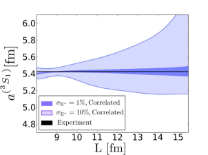
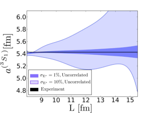
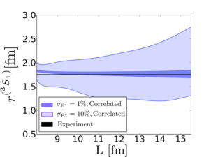
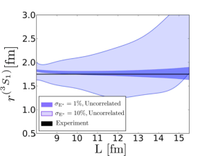
Figure 7: The values of $\{a^{(^{3}S_{1})},r^{(^{3}S_{1})}\}$ obtained by fitting the six independent bound-state energies with $|\textbf{d}|\leq\sqrt{3}$ (depicted in Figs. 3, 4, 5), generated from synthetic LQCD calculations, using the approximate QCs in Eqs. (17-22), as discussed in the text. The black lines denote the experimental value of these quantities determined by fitting the scattering parameters obtained from Ref. NIJ . The dark (light) inner (outer) band is the $1\sigma$ band corresponding to the energies being determined with 1% (10%) precision.

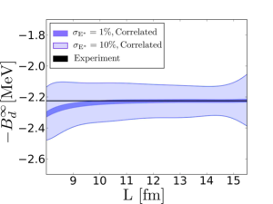
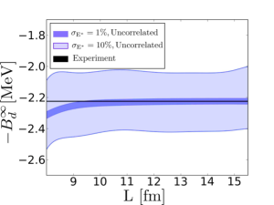
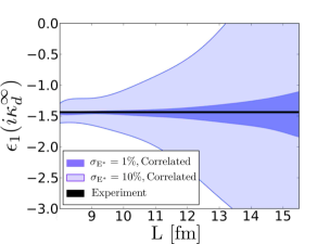
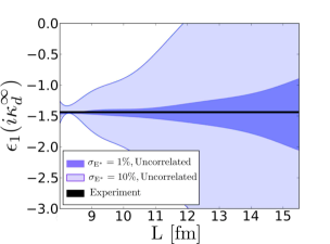
Figure 8: The values of $\{-B_{d}^{\infty},\epsilon_{1}(\mathit{i}\kappa_{d}^{\infty})\}$ obtained by fitting the six independent bound-state energies with $|\textbf{d}|\leq\sqrt{3}$ (depicted in Figs. 3, 4, 5), generated from synthetic LQCD calculations, using the approximate QCs in Eqs. (17-22). $\epsilon_{1}$ is in degrees and ${B_{d}^{\infty}}(\kappa_{d}^{\infty})$ denotes the infinite-volume deuteron binding energy (momentum). The black lines denote the experimental value of these quantities determined by fitting the scattering parameters obtained from Ref. NIJ . The dark (light) inner (outer) band is the $1\sigma$ band corresponding to the energies being determined with 1% (10%) precision.

Using the QCs, the ground-state energy in each irrep is determined for a given lattice volume. The level of precision of such a future LQCD calculation is introduced by selecting a modified energy for each ground state from a Gaussian distribution with the true energy for its mean and the precision level multiplied by the mean for its standard deviation. This generates one set of uncorrelated “synthetic LQCD calculations”. To generate fully correlated “synthetic LQCD calculations”, the same fluctuation (appropriately scaled) is chosen for each energy.  These synthetic data are then taken to be the results of a possible future LQCD calculation and analyzed accordingly to extract the scattering parameters. The values of $\{a^{(^{3}S_{1})},r^{(^{3}S_{1})},-B_{d}^{\infty},\epsilon_{1}(\mathit{i}\kappa_{d}^{\infty})\}$ extracted from an analysis of the synthetic data are shown in Figs. 7, 8 for both correlated and uncorrelated energies. Since for ${\rm L}\lesssim 10~{}\rm{fm}$ the contribution of the D-wave phase shifts to the bound-state spectrum is not negligible, the mean values of the scattering parameters extracted using the approximated QCs deviate from their experimental values. This is most noticeable when the binding energies are determined at the 1% level of precision, where the S-matrix parameters and predicted $B_{d}^{\infty}$ can deviate by $\sim 3\sigma$ from the experimental values for this range of volumes. For $10~{}\rm{fm}$$<{\rm L}<$$14~{}\rm{fm}$, one can see that these quantities can be extracted with high accuracy using this method, but it is important to note that the precision with which $\{a^{(^{3}S_{1})},r^{(^{3}S_{1})},\epsilon_{1}(\mathit{i}\kappa_{d}^{\infty)}\}$ can be extracted decreases as a function of increasing volume. The reason is that the bound-state energy in each irrep asymptotes to the physical deuteron binding energy in the infinite-volume limit. In this limit, sensitivity to $\epsilon_{1}$ is lost and the $\alpha$-wave phase shift is determined at a single energy, the deuteron pole. Therefore, for sufficiently large volumes one cannot independently resolve $a^{(^{3}S_{1})}$ and $r^{(^{3}S_{1})}$. This analysis of synthetic data reinforces the fact that the FV spectrum not only depends on the magnitude of $\epsilon_{1}$ but also its sign. As discussed in Sect. II, this sensitivity can be deduced from the full QCs in Eqs.(42-168), but it is most evident from the approximated QCs in Eqs. (17-22).

In performing this analysis, we have benefited from two important pieces of apriori knowledge at the physical light-quark masses. First is that in the volumes of interest, the bound-state energy in each irrep falls within the radius of convergence of the ERE, $|{\rm E}^{*}|<m_{\pi}^{2}/4M$. For unphysical light-quark masses, the S-matrix elements could in principle change in such a way that this need not be the case and pionful EFTs would be required to extract the scattering parameters from the FV spectrum. Second is that the D-wave phase shifts are naturally small. Again, since the dependence of these phase shifts on the light-quark masses can only be estimated, further investigation would be required. To improve upon this analysis, the J=1 $\beta$-wave and $J=2,3$ D-wave phase shifts would have to be extracted from the scattering states. As is evident from Fig. 2, states that have a strong dependence on the D-wave phase shifts will, in general, lie above the t-channel cut. In principle, one could attempt to extract them by fitting the FV bound-state energies for ${\rm L}\leq 10~{}{\rm fm}$ with the full QCs. In practice, this will be challenging as eight scattering parameters appear in the ERE at the order at which the $J=1$ $\beta$-wave and $J=2,3$ D-wave phase shifts first contribute. This is also formally problematic since for small volumes, $m_{\pi}{\rm L}\raisebox{-3.01385pt}{$\stackrel{{\scriptstyle\textstyle<}}{{\sim}}$ }2\pi$, finite range effects are no longer negligible. Although these finite range effects have been estimated for two nucleons in a S-wave Sato and Bedaque (2007), they remain to be examined for the general NN system.

IV The Finite-Volume Deuteron Wavefunction and the Asymptotic D/S Ratio

The S-matrix dictates the asymptotic behavior of the NN wavefunction, and as a result the infra-red (IR) distortions of the wavefunction inflicted by the boundaries of the lattice volume have a direct connection to the parameters of the scattering matrix, as exploited by Lüscher. Outside the range of the nuclear forces, the FV wavefunction of the NN system is obtained from the solution of the Helmholtz equation in a cubic volume with the PBCs Luscher (1986, 1991); Rummukainen and Gottlieb (1995); Ishizuka (2009). By choosing the amplitude of the $l=0$ and $l=2$ components of the FV wavefunction to recover the asymptotic D/S ratio of the infinite-volume deuteron, it is straightforward to show Luscher (1986, 1991) that the unnormalized FV deuteron wavefunctions associated with the approximate QCs in Eqs. (17-22) are

$$\psi^{V,{\bf d}}_{1,M_{J}}(\mathbf{r};\kappa)\ =\ \psi^{\infty}_{1,M_{J}}(\mathbf{r};\kappa)\ +\ \sum_{\mathbf{n}\neq\mathbf{0}}e^{i\pi\mathbf{n}\cdot\mathbf{d}}\ \psi^{\infty}_{1,M_{J}}(\mathbf{r}+\mathbf{n}{\rm L};\kappa)\ \ \ ,$$ (25)

with $r=|{\bf r}|>R$, where $\mathbf{r}$ denotes the relative displacement of the two nucleons, and $R>>1/m_{\pi}$ is the approximate range of the nuclear interactions. The subscripts on the wavefunction refer to the $J=1,~{}M_{J}=0,\pm 1$ quantum numbers of the state and $\mathbf{n}$ is an integer triplet. In order for Eq. (25) to be an energy eigenstate of the Hamiltonian, $E^{*}=-{\kappa^{2}}/{M}$ has to be an energy eigenvalue of the NN system in the finite volume, obtained from the QCs in Eqs. (17-22). $\psi^{\infty}_{1,M_{J}}(\mathbf{r})$ is the asymptotic infinite-volume wavefunction of the deuteron,

$$\psi^{\infty}_{1,M_{J}}(\mathbf{r};\kappa)\ =\ \mathcal{A}_{S}\ \left(\ \frac{e^{-\kappa r}}{r}\mathcal{Y}_{1M_{J};01}(\hat{\mathbf{r}})\ +\ \eta~{}\frac{e^{-\kappa r}}{r}(1+\frac{3}{\kappa r}+\frac{3}{\kappa^{2}r^{2}})\mathcal{Y}_{1M_{J};21}(\hat{\mathbf{r}})\ \right)\ \ \ .$$ (26)

with $\mathcal{Y}_{JM_{J};L1}$ being the well-known spin-orbital functions,

$$\mathcal{Y}_{JM_{J};L1}(\hat{\mathbf{r}})\ =\ \sum_{M_{L},M_{S}}\left\langle LM_{L}1M_{S}|JM_{J}\right\rangle\ Y_{LM_{L}}(\hat{\mathbf{r}})\ \mathcal{\chi}_{1M_{S}}\ \ \ ,$$ (27)

where $\mathcal{\chi}_{1M_{S}}$ is the spin wavefunction of the deuteron. $\eta$ is the deuteron asymptotic D/S ratio which is related to the mixing angle via $\eta=-\tan{\epsilon_{1}}|_{k^{*}=i\kappa^{\infty}_{d}}$ Blatt and Biedenharn (1952). As is well known from the effective range theory Bethe (1949); Bethe and Longmire (1950), the short-distance contribution to the outer quantities of the deuteron, such as the quadrupole moment, can be approximately taken into account by requiring the normalization of the asymptotic wavefunction of the deuteron, obtained from the residue of the S-matrix at the deuteron pole, to be approximately $|\mathcal{A}_{S}|^{2}\approx{2\kappa}/({1-\kappa r^{(^{3}S_{1})}})$. Corrections to this normalization arise at $\mathcal{O}\left({\kappa^{3}}/{R}^{2},\kappa\eta^{2}\right)$, at the same order the $J=1$ $\beta$-wave and $J=2,3$ D-waves contribute. In writing the FV wavefunction in Eq. (25) contributions from these waves have been neglected.

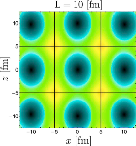
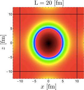
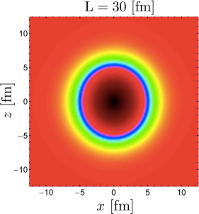
Figure 9: The mass density in the $xz$-plane from the $\mathbb{T}_{1}$ FV deuteron wavefunction at rest for ${\rm L}=10,15,20$, and $30~{}{\rm fm}$.

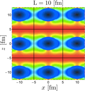
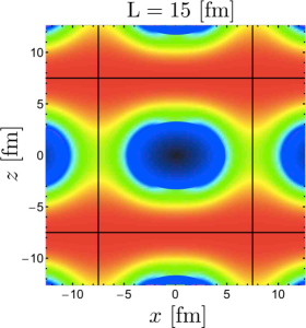
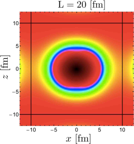
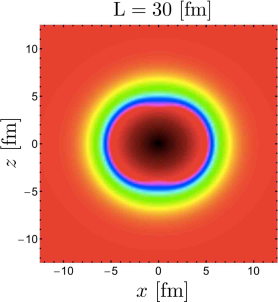
Figure 13: The mass density in the $xz$-plane from the $\mathbb{A}_{2}$ FV deuteron wavefunction with $\mathbf{d}=(0,0,1)$.

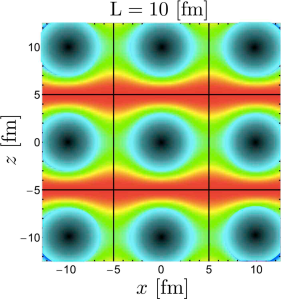
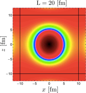
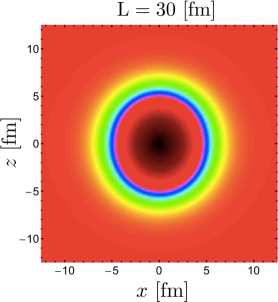
Figure 14: The mass density in the $xz$-plane from the $\mathbb{E}$ FV deuteron wavefunction with $\mathbf{d}=(0,0,1)$.

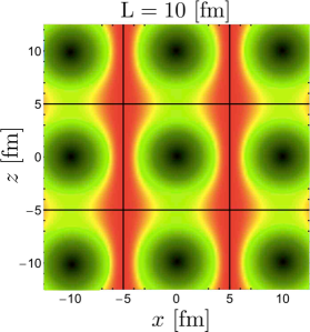
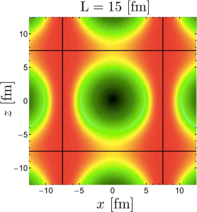
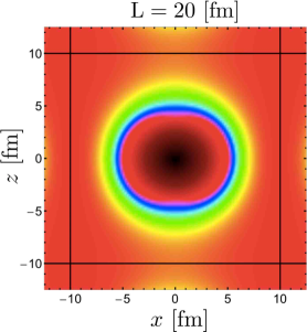
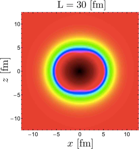
Figure 15: The mass density in the $xz$-plane from the $\mathbb{B}_{1}$ FV deuteron wavefunction with $\mathbf{d}=(1,1,0)$.

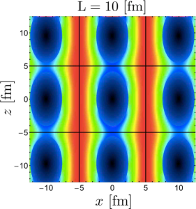
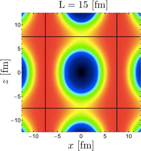
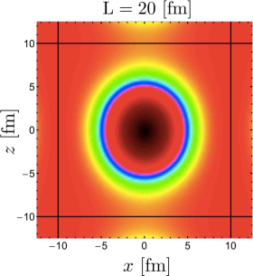
Figure 16: The mass density in the $xz$-plane from the $\mathbb{B}_{2}/\mathbb{B}_{3}$ FV deuteron wavefunction with $\mathbf{d}=(1,1,0)$.

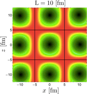
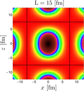
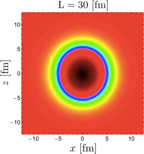
Figure 17: The mass density in the $xz$-plane from the $\mathbb{A}_{2}/\mathbb{E}$ FV deuteron wavefunction with $\mathbf{d}=(1,1,1)$.

An important feature of the FV wavefunction in Eq. (25) is the contribution from partial waves other than $l=0$ and $l=2$, which results from the cubic distribution of the periodic images. While there are also FV corrections to the $l=0$ component of the wavefunction, the FV corrections to the $l=2$ component are enhanced for systems with ${\bf d}=(0,0,1)$ and $(1,1,0)$. By forming appropriate linear combinations of the $\psi^{V,{\bf d}}_{1,M_{J}}$ that transform according to a given irrep of the cubic, tetragonal, orthorhombic and trigonal point groups (see Table 2), wavefunctions for the systems with ${\bf d}=(0,0,0)$, $(0,0,1)$, $(1,1,0)$ and $(1,1,1)$ can be obtained. The mass density in the $xz$-plane from the FV wavefunction of the deuteron at rest in the volume, obtained from the $\mathbb{T}_{1}$ irrep of the cubic group is shown in Fig. 9 for ${\rm L}=10,15,20$, and $30~{}{\rm fm}$, and for the boosted systems in Figs. 13-17 of Appendix C. As the interior region of the wavefunctions cannot be deduced from its asymptotic behavior alone, it is “masked” in Fig. 9 and Figs. 13-17 by a shaded disk. Although the deuteron wavefunction exhibits its slight prolate shape (with respect to its spin axis) at large volumes, it is substantially deformed in smaller volumes, such that the deuteron can no longer be thought as a compact bound state within the lattice volume. When the system is at rest, the FV deuteron is more prolate than the infinite-volume deuteron. When the deuteron is boosted along the $z$-axis with ${\bf d}=(0,0,1)$, the distortion of the wavefunction is large, and in fact, for a significant range of volumes (${\rm L}\lesssim 30~{}\rm{fm}$), the FV effects give rise to an oblate (as opposed to prolate) deuteron in the $\mathbb{E}$ irrep, Fig. 14, and a more prolate shape in the $\mathbb{A}_{2}$ irrep, Fig. 13. For ${\bf d}=(1,1,0)$, the system remains prolate for the deuteron in the $\mathbb{B}_{2}/\mathbb{B}_{3}$ irreps, Fig. 16, while it becomes oblate in the $\mathbb{B}_{1}$ irrep, Fig. 15, for volumes up to ${\rm L}\sim 30~{}\rm{fm}$.

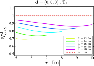
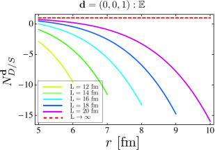
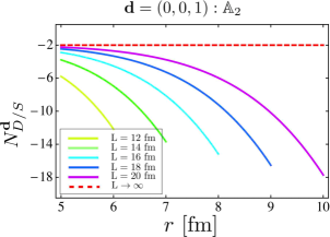
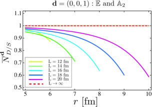
Figure 10: The normalized D/S ratio of the deuteron wavefunction with $M_{J}=M_{S}=1$, defined in Eq. (28) and Eq. (29) in the (a) $\mathbb{T}_{1}$, (b) $\mathbb{E}$ and (c) with $M_{J}=M_{S}=0$ in the $\mathbb{A}_{2}$ irrep, along with (d) the difference of the D/S ratios in the $\mathbb{E}$ and $\mathbb{A}_{2}$ irreps, defined in Eq. (30). The red-dashed lines show the infinite-volume value.

Although the normalization factor $\mathcal{A}_{S}$ corrects for the fact that the complete wavefunction is not given by the asymptotic form given in Eq. (26) for $|{\bf r}|\lesssim r^{(^{3}S_{1})}/2$ in infinite volume, it gives rise to a normalization ambiguity in the FV. On the other hand, the asymptotic D/S ratio is protected by the S-matrix, and can be directly extracted from the long-distance tail of the lattice wavefunctions.  It is evident from Eq. (26) that the ratio

$$N_{D/S}^{{\bf d};M_{J},M_{S}}(r;\kappa)\equiv\frac{\psi_{D;M_{J},M_{S}}^{V,{\bf d}}(r;\kappa)}{\eta~{}\chi(r;\kappa)~{}\psi_{S;M_{J},M_{S}}^{V,{\bf d}}(r;\kappa)}\ \ \ ,$$ (28)

with $\chi(r;\kappa)=\sqrt{\frac{1}{10}}(1+\frac{3}{\kappa r}+\frac{3}{\kappa^{2}r^{2}})$, is unity for the $M_{J}=M_{S}=1$ component of the infinite-volume deuteron wavefunction (and is equal to $-2$ for the $M_{J}=M_{S}=0$ component), where $\psi_{S;M_{J},M_{S}}^{V,{\bf d}}$ and $\psi_{D;M_{J},M_{S}}^{V,{\bf d}}$ are

$$\psi_{S;M_{J},M_{S}}^{V,{\bf d}}(r;\kappa) = \int d\Omega_{\hat{\mathbf{r}}}\ \psi^{V,{\bf d}}_{1,M_{J}}(\mathbf{r},\kappa)\big{|}_{M_{S}}\ \ Y_{00}(\hat{\mathbf{r}})\ ,$$

$$\psi_{D;M_{J},M_{S}}^{V,{\bf d}}(r;\kappa) = \int d\Omega_{\hat{\mathbf{r}}}\ \psi^{V,{\bf d}}_{1,M_{J}}(\mathbf{r},\kappa)\big{|}_{M_{S}}\ \ Y_{20}(\hat{\mathbf{r}})\ ,$$ (29)

with $r\leq{\rm L}/2$. By evaluating the FV wavefunction in different irreps with $|\mathbf{d}|\leq\sqrt{3}$, this ratio can be determined in the FV, as is shown in Fig. 10. Not only does it exhibit strong dependence on the volume, but also varies dramatically as a function of $r$. This is due to the fact that the periodic images give rise to exponentially growing contributions to the FV wavefunction in $r$. For the FV deuteron at rest and with $\mathbf{d}=(1,1,1)$, a sufficiently small $r$ gives rise to a $N_{D/S}^{{\bf d};M_{J},M_{S}}$ that is not severely distorted by volume effects even in small volumes. In contrast, this ratio deviates significantly from its infinite-volume value for systems with $\mathbf{d}=(0,0,1)$ and $(1,1,0)$ even in large volumes (${\rm L}\lesssim 20~{}\rm{fm}$). This feature is understood by noting that while the leading correction to $N_{D/S}^{{\bf d};M_{J},M_{S}}$ is $\sim\eta~{}e^{-\kappa{\rm L}}$ for systems with ${\bf d}=(0,0,0)$ and $(1,1,1)$, they are $\sim e^{-\kappa{\rm L}}$ for systems with ${\bf d}=(0,0,1)$ and $(1,1,0)$. The periodic images of the wavefunction with the latter boosts are quadrupole distributed, and consequently modify the $l=2$ component of the wavefunction by contributions that are not suppressed by $\eta$. However, for these systems, there are two irreps that receive similar FV corrections to their ratios, which can be largely removed by forming differences, e.g. for the system with ${\bf d}=(0,0,1)$,

$$\overline{N}_{D/S}^{(0,0,1)} = {1\over 3}\left(N_{D/S}^{(0,0,1);1,1}\ -\ N_{D/S}^{(0,0,1);0,0}\right)\ =\ {1\over 3}\left(N_{D/S}^{(0,0,1);\mathbb{E}}\ -\ N_{D/S}^{(0,0,1);\mathbb{A}_{2}}\right)\ \ \ ,$$ (30)

as shown in Fig. 10. A similar improvement is found for systems with ${\bf d}=(1,1,0)$. It is also worth noting that the contributions to the wavefunction from higher partial waves, $l\geq 2$, can be added to $\psi^{V,{\bf d}}$ with coefficients that depend on their corresponding phase shifts, and therefore are small under the assumption of low-energy scattering Luscher (1991); Rummukainen and Gottlieb (1995); Ishizuka (2009). However, the partial-wave decomposition of the FV wavefunction in Eq. (25) contains contributions with $l\geq 2$. In the limit where the corresponding phase shifts vanish, the wavefunction, in contrast to the spectrum, remains sensitive to these contributions, resulting in the larger FV modifications of quantities compared with their spectral analogues.

An extraction of $\eta$ is possible by taking sufficiently large volumes such that a large NN separation can be achieved without approaching the boundaries of the volume. While the wavefunctions corresponding to the deuteron at rest or with $\mathbf{d}=(1,1,1)$ provide an opportunity to extract $\eta$ with an accuracy of $\sim 15-20\%$ in volumes of ${\rm L}\sim 14~{}\rm{fm}$, combinations of the ratios obtained from the two irreps in both the systems with $\mathbf{d}=(0,0,1)$ and $(1,1,0)$ will provide for a $\sim 10\%$ determination in volumes of ${\rm L}\sim 12~{}\rm{fm}$, as shown in Fig. 10. As it is possible that the uncertainties in the extraction of $\eta$ can be systematically reduced, those due to the neglect of the $J=1$ $\beta$-wave and $J=2,3$ D-wave phase shifts, as well as higher order terms in the ERE, deserve further investigation.

V Summary and Conclusion

A Lattice QCD calculation of the deuteron and its properties would be a theoretical milestone on the path toward calculating quantities of importance in low-energy nuclear physics from quantum chromodynamics without uncontrolled approximations or assumptions. While there is no formal impediment to calculating the deuteron binding energy to arbitrary precision when sufficient computational resources become available, determining its properties and interactions presents a challenge that has largely remained unexplored Detmold and Savage (2004); Meyer (2012); Briceno et al. . As LQCD calculations are performed in a finite Euclidean spacetime volume with certain boundary conditions imposed upon the fields, calculating the properties of the deuteron requires establishing a rigorous connection between FV correlation functions and the S-matrix. Using the NN formalism developed in Ref. Briceno et al. , we have explored the FV energy spectra of states that have an overlap with the ${}^{3}\hskip-1.8063ptS_{1}$-${}^{3}\hskip-1.8063ptD_{1}$ coupled-channels system in which the deuteron resides. Although the full FV QCs associated with the ${}^{3}S_{1}$-${}^{3}D_{1}$ coupled channels depend on interactions in all positive-parity isoscalar channels, a low-energy expansion depends only on four scattering phases and one mixing angle. Further, for the deuteron, these truncated QCs can be further simplified to depend only upon one phase shift and the mixing angle, with corrections suppressed by $\sim\frac{1}{\rm L}e^{-2\kappa{\rm L}}\tan{\delta_{i}}$ where $\delta_{i}$ denotes the $J=1$ $\beta$-wave and $J=2,3$ D-wave phase shifts which are all small at the deuteron binding energy. We have demonstrated that the infinite-volume deuteron binding energy and leading scattering parameters, including the mixing angle, $\epsilon_{1}$, that dictate the low-energy behavior of the scattering amplitudes, can be (in principle) determined with precision from the bound-state spectra of deuterons, both at rest and in motion, in a single modest volume, with ${\rm L}=10$-$14~{}\rm{fm}$. Calculations in a second lattice volume would reduce the systematic uncertainties introduced by truncating the QCs.

We have investigated the feasibility of extracting $\epsilon_{1}$ from the asymptotic D/S ratio of the deuteron FV wavefunction using the periodic images associated with the $\alpha$-wavefunction. As the amplitude of the $J=1$ $\beta$-wave and the $J=2,3$ D-wave components of the wavefunction are not constrained by the infinite-volume deuteron wavefunction, the analysis is limited by an imposed truncation of the ERE, which is at the same level of approximation as the approximate QCs. The systematic uncertainties introduced by this truncation are currently unknown, but will be suppressed by the small phase shifts in those channels in addition to being exponentially suppressed with ${\rm L}$. This is in contrast to the extraction from the FV spectra where the systematic uncertainties have been determined to be small. With this approximation, it is estimated that volumes with ${\rm L}\raisebox{-3.01385pt}{$\stackrel{{\scriptstyle\textstyle>}}{{\sim}}$ }12~{}\rm{fm}$ are required to extract $\epsilon_{1}$ with $\sim 10\%$ level of accuracy from the asymptotic form of the wavefunctions.

Acknowledgment

RB, ZD and MJS were supported in part by the DOE grant No. DE-FG02-97ER41014. ZD and MJS were also supported in part by DOE grant No. DE-FG02-00ER41132. The work of TL was performed under the auspices of the U.S. Department of Energy by Lawrence Livermore National Laboratory under Contract DE-AC52-07NA27344.

Appendix A Quantization Conditions

The NN FV QCs in the positive-parity isoscalar channels that have an overlap with ${}^{3}\hskip-1.8063ptS_{1}$-${}^{3}\hskip-1.8063ptD_{1}$ coupled channels are listed in this appendix for a number of CM boosts. With the notation introduced in Ref. Briceno et al. , the QC for the irrep $\Gamma_{i}$ can be written as

$$\det\left({\mathbb{M}}^{(\Gamma_{i})}+\frac{iMk^{*}}{4\pi}-\mathcal{F}^{(\Gamma_{i}),{\textbf{d}}}\right)=0\ \ \ ,$$ (31)

where

$$\mathcal{F}^{(\Gamma_{i}),{\textbf{d}}}(k^{*2};{\rm L}) = {M}\sum_{l,m}\frac{1}{k^{*l}}~{}{\mathbb{F}}_{lm}^{(\Gamma_{i})}~{}{c_{lm}^{\textbf{d}}(k^{*2};{\rm L})}\ \ \ ,$$

$${\mathbb{M}}^{(\Gamma_{i})} = \left(\mathcal{M}^{-1}\right)_{\Gamma_{i}}\ \ \ ,$$ (32)

where the functions ${c_{lm}^{\textbf{d}}(k^{*2};{\rm L})}$ are defined in Eq. (3), $M$ is the nucleon mass and $k^{*}$ is the on-shell momentum of each nucleon in the CM frame. It is straightforward to decompose $\mathcal{M}^{-1}$ into $\left(\mathcal{M}^{-1}\right)_{\Gamma_{i}}$ using the eigenvectors of the FV functions. The matrices $\mathbb{F}$ and $\mathbb{M}$ are given in the following subsections.

For notational convenience, $\mathcal{M}_{1,S(D)}$ denotes the scattering amplitude in the channel with total angular momentum $J=1$ and orbital angular momentum $L=0~{}(L=2)$, $\mathcal{M}_{1,SD}$ is the amplitude between $S$ and $D$ partial waves in the $J=1$ channel, and $\text{det}\mathcal{M}_{1}$ is the determinant of the $J=1$ sector of the scattering-amplitude matrix,

$$\det\mathcal{M}_{1}=\det\left(\begin{array}[]{cc}\mathcal{M}_{1,S}&\mathcal{M}_{1,SD}\\ \mathcal{M}_{1,DS}&\mathcal{M}_{1,D}\\ \end{array}\right)\ \ \ .$$ (35)

A.0.1 $\mathbf{d}=(0,0,0)$

$$\mathbb{T}_{1}:\hskip 14.22636pt\mathbb{F}_{00}^{(\mathbb{T}_{1})}=\textbf{I}_{3},\hskip 14.22636pt\mathbb{F}_{40}^{(\mathbb{T}_{1})}=\left(\begin{array}[]{ccc}0&0&0\\ 0&0&\frac{2\sqrt{6}}{7}\\ 0&\frac{2\sqrt{6}}{7}&\frac{2}{7}\\ \end{array}\right),\hskip 14.22636pt{\mathbb{M}}^{(\mathbb{T}_{1})}=\left(\begin{array}[]{ccc}\frac{\mathcal{M}_{1,D}}{{\det\mathcal{M}_{1}}}&-\frac{\mathcal{M}_{1,SD}}{\det\mathcal{M}_{1}}&0\\ -\frac{\mathcal{M}_{1,SD}}{\det\mathcal{M}_{1}}&\frac{\mathcal{M}_{1,S}}{\det\mathcal{M}_{1}}&0\\ 0&0&\mathcal{M}_{3,D}^{-1}\\ \end{array}\right).$$ (42)

A.0.2 $\mathbf{d}=(0,0,1)$

$$\mathbb{A}_{2}:\hskip 14.22636pt\mathbb{F}_{00}^{(\mathbb{A}_{2})}=\textbf{I}_{3}\ \ ,\hskip 14.22636pt\mathbb{F}_{20}^{(\mathbb{A}_{2})}=\left(\begin{array}[]{ccc}\frac{2}{\sqrt{5}}&0&-\frac{9}{7\sqrt{5}}\\ 0&-\frac{1}{\sqrt{5}}&\frac{6}{7}\sqrt{\frac{2}{5}}\\ -\frac{9}{7\sqrt{5}}&\frac{6}{7}\sqrt{\frac{2}{5}}&\frac{8}{7\sqrt{5}}\\ \end{array}\right),\hskip 14.22636pt\mathbb{F}_{40}^{(\mathbb{A}_{2})}=\left(\begin{array}[]{ccc}0&0&-\frac{4}{7}\\ 0&0&-\frac{2\sqrt{2}}{7}\\ -\frac{4}{7}&-\frac{2\sqrt{2}}{7}&\frac{2}{7}\\ \end{array}\right),$$ (49)

$$\hskip 28.45274pt{\mathbb{M}}^{(\mathbb{A}_{2})}=\left(\begin{array}[]{ccc}\frac{2\mathcal{M}_{1,S}+2\sqrt{2}\mathcal{M}_{1,SD}+\mathcal{M}_{1,D}}{3\det\mathcal{M}_{1}}&\frac{\sqrt{2}\mathcal{M}_{1,S}-\mathcal{M}_{1,SD}-\sqrt{2}\mathcal{M}_{1,D}}{3\det\mathcal{M}_{1}}&0\\ \frac{\sqrt{2}\mathcal{M}_{1,S}-\mathcal{M}_{1,SD}-\sqrt{2}\mathcal{M}_{1,D}}{3\det\mathcal{M}_{1}}&\frac{\mathcal{M}_{1,S}-2\sqrt{2}\mathcal{M}_{1,SD}+2\mathcal{M}_{1,D}}{3\det\mathcal{M}_{1}}&0\\ 0&0&\mathcal{M}_{3,D}^{-1}\\ \end{array}\right).$$ (53)

$$E:\hskip 14.22636pt\mathbb{F}_{00}^{(\mathbb{E})}=\textbf{I}_{5}\ \ \ ,\hskip 14.22636pt\mathbb{F}_{20}^{(\mathbb{E})}=\left(\begin{array}[]{ccccc}\frac{1}{2\sqrt{5}}&0&-\frac{\sqrt{3}}{2}&0&\frac{4\sqrt{\frac{3}{5}}}{7}\\ 0&-\frac{1}{\sqrt{5}}&0&0&-\frac{3}{7}\sqrt{\frac{6}{5}}\\ -\frac{\sqrt{3}}{2}&0&\frac{\sqrt{5}}{14}&0&-\frac{2}{7}\\ 0&0&0&-\frac{2}{7}\sqrt{5}&0\\ \frac{4\sqrt{\frac{3}{5}}}{7}&-\frac{3}{7}\sqrt{\frac{6}{5}}&-\frac{2}{7}&0&\frac{6}{7\sqrt{5}}\\ \end{array}\right),$$ (59)

$$\hskip 28.45274pt\mathbb{F}_{40}^{(\mathbb{E})}=\left(\begin{array}[]{ccccc}0&0&0&0&\frac{\sqrt{3}}{7}\\ 0&0&0&0&\frac{\sqrt{6}}{7}\\ 0&0&\frac{8}{21}&0&-\frac{5\sqrt{5}}{21}\\ 0&0&0&\frac{1}{7}&0\\ \frac{\sqrt{3}}{7}&\frac{\sqrt{6}}{7}&-\frac{5\sqrt{5}}{21}&0&\frac{1}{21}\end{array}\right),\hskip 14.22636pt\mathbb{F}_{44}^{(\mathbb{E})}=\left(\begin{array}[]{ccccc}0&0&0&\sqrt{\frac{2}{7}}&0\\ 0&0&0&\frac{2}{\sqrt{7}}&0\\ 0&0&0&\sqrt{\frac{10}{21}}&0\\ \sqrt{\frac{2}{7}}&\frac{2}{\sqrt{7}}&\sqrt{\frac{10}{21}}&0&\sqrt{\frac{2}{21}}\\ 0&0&0&\sqrt{\frac{2}{21}}&0\end{array}\right),$$ (70)

$$\hskip 28.45274pt{\mathbb{M}}^{(\mathbb{E})}=\left(\begin{array}[]{ccccc}\frac{\mathcal{M}_{1,S}-2\sqrt{2}\mathcal{M}_{1,SD}+2\mathcal{M}_{1,D}}{3\det\mathcal{M}_{1}}&\frac{\sqrt{2}\mathcal{M}_{1,S}-\mathcal{M}_{1,SD}-\sqrt{2}\mathcal{M}_{1,D}}{3\det\mathcal{M}_{1}}&0&0&0\\ \frac{\sqrt{2}\mathcal{M}_{1,S}-\mathcal{M}_{1,SD}-\sqrt{2}\mathcal{M}_{1,D}}{3\det\mathcal{M}_{1}}&\frac{2\mathcal{M}_{1,S}+2\sqrt{2}\mathcal{M}_{1,SD}+\mathcal{M}_{1,D}}{3\det\mathcal{M}_{1}}&0&0&0\\ 0&0&\mathcal{M}_{2,D}^{-1}&0&0\\ 0&0&0&\mathcal{M}_{3,D}^{-1}&0\\ 0&0&0&0&\mathcal{M}_{3,D}^{-1}\\ \end{array}\right).$$ (76)

A.0.3 $\mathbf{d}=(1,1,0)$

$$\mathbb{B}_{1}:\hskip 14.22636pt\mathbb{F}_{00}^{(\mathbb{B}_{1})}=\textbf{I}_{5}\ \ \ ,\hskip 14.22636pt\mathbb{F}_{20}^{(\mathbb{B}_{1})}=\left(\begin{array}[]{ccccc}\frac{2}{\sqrt{5}}&0&0&-\frac{9}{7\sqrt{5}}&0\\ 0&-\frac{1}{\sqrt{5}}&0&\frac{6}{7}\sqrt{\frac{2}{5}}&0\\ 0&0&-\frac{\sqrt{5}}{7}&0&-\frac{\sqrt{10}}{7}\\ -\frac{9}{7\sqrt{5}}&\frac{6}{7}\sqrt{\frac{2}{5}}&0&\frac{8}{7\sqrt{5}}&0\\ 0&0&-\frac{\sqrt{10}}{7}&0&0\\ \end{array}\right),$$ (82)

$$\hskip 28.45274pt\mathbb{F}_{40}^{(\mathbb{B}_{1})}=\left(\begin{array}[]{ccccc}0&0&0&-\frac{4}{7}&0\\ 0&0&0&-\frac{2\sqrt{2}}{7}&0\\ 0&0&-\frac{2}{21}&0&\frac{5\sqrt{2}}{21}\\ -\frac{4}{7}&-\frac{2\sqrt{2}}{7}&0&\frac{2}{7}&0\\ 0&0&\frac{5\sqrt{2}}{21}&0&-\frac{1}{3}\\ \end{array}\right),\hskip 14.22636pt\mathbb{F}_{44}^{(\mathbb{B}_{1})}=\left(\begin{array}[]{ccccc}0&0&0&0&0\\ 0&0&0&0&0\\ 0&0&-\frac{2}{3}\sqrt{\frac{10}{7}}&0&-\frac{2}{3}\sqrt{\frac{5}{7}}\\ 0&0&0&0&0\\ 0&0&-\frac{2}{3}\sqrt{\frac{5}{7}}&0&-\frac{\sqrt{\frac{10}{7}}}{3}\\ \end{array}\right),$$ (93)

$$\hskip 28.45274pt{\mathbb{M}}^{(\mathbb{B}_{1})}=\left(\begin{array}[]{ccccc}\frac{2\mathcal{M}_{1,S}+2\sqrt{2}\mathcal{M}_{1,SD}+\mathcal{M}_{1,D}}{3\det\mathcal{M}_{1}}&\frac{\sqrt{2}\mathcal{M}_{1,S}-\mathcal{M}_{1,SD}-\sqrt{2}\mathcal{M}_{1,D}}{3\det\mathcal{M}_{1}}&0&0&0\\ \frac{\sqrt{2}\mathcal{M}_{1,S}-\mathcal{M}_{1,SD}-\sqrt{2}\mathcal{M}_{1,D}}{3\det\mathcal{M}_{1}}&\frac{\mathcal{M}_{1,S}-2\sqrt{2}\mathcal{M}_{1,SD}+2\mathcal{M}_{1,D}}{3\det\mathcal{M}_{1}}&0&0&0\\ 0&0&\mathcal{M}_{2,D}^{-1}&0&0\\ 0&0&0&\mathcal{M}_{3,D}^{-1}&0\\ 0&0&0&0&\mathcal{M}_{3,D}^{-1}\\ \end{array}\right).$$ (99)

$$\mathbb{B}_{2}:\hskip 14.22636pt\mathbb{F}_{00}^{(\mathbb{B}_{2})}=\textbf{I}_{5}\ \ \ ,\hskip 14.22636pt\mathbb{F}_{20}^{(\mathbb{B}_{2})}=\left(\begin{array}[]{ccccc}-\frac{1}{\sqrt{5}}&0&0&0&-\frac{3}{7}\sqrt{\frac{6}{5}}\\ 0&\frac{1}{2\sqrt{5}}&-\frac{\sqrt{3}}{2}&0&\frac{4\sqrt{\frac{3}{5}}}{7}\\ 0&-\frac{\sqrt{3}}{2}&\frac{\sqrt{5}}{14}&0&-\frac{2}{7}\\ 0&0&0&-\frac{2\sqrt{5}}{7}&0\\ -\frac{3}{7}\sqrt{\frac{6}{5}}&\frac{4\sqrt{\frac{3}{5}}}{7}&-\frac{2}{7}&0&\frac{6}{7\sqrt{5}}\\ \end{array}\right),$$ (105)

$$\hskip 28.45274pt\mathbb{F}_{40}^{(\mathbb{B}_{2})}=\left(\begin{array}[]{ccccc}0&0&0&0&\frac{\sqrt{6}}{7}\\ 0&0&0&0&\frac{\sqrt{3}}{7}\\ 0&0&\frac{8}{21}&0&-\frac{5\sqrt{5}}{21}\\ 0&0&0&\frac{1}{7}&0\\ \frac{\sqrt{6}}{7}&\frac{\sqrt{3}}{7}&-\frac{5\sqrt{5}}{21}&0&\frac{1}{21}\\ \end{array}\right),\hskip 14.22636pt\mathbb{F}_{44}^{(\mathbb{B}_{2})}=\left(\begin{array}[]{ccccc}0&0&0&\frac{2i}{\sqrt{7}}&0\\ 0&0&0&i\sqrt{\frac{2}{7}}&0\\ 0&0&0&i\sqrt{\frac{10}{21}}&0\\ -\frac{2i}{\sqrt{7}}&-i\sqrt{\frac{2}{7}}&-i\sqrt{\frac{10}{21}}&0&-i\sqrt{\frac{2}{21}}\\ 0&0&0&i\sqrt{\frac{2}{21}}&0\\ \end{array}\right),$$ (116)

$$\hskip 28.45274pt{\mathbb{M}}^{(\mathbb{B}_{2})}=\left(\begin{array}[]{ccccc}\frac{2\mathcal{M}_{1,S}+2\sqrt{2}\mathcal{M}_{1,SD}+\mathcal{M}_{1,D}}{3\det\mathcal{M}_{1}}&\frac{\sqrt{2}\mathcal{M}_{1,S}-\mathcal{M}_{1,SD}-\sqrt{2}\mathcal{M}_{1,D}}{3\det\mathcal{M}_{1}}&0&0&0\\ \frac{\sqrt{2}\mathcal{M}_{1,S}-\mathcal{M}_{1,SD}-\sqrt{2}\mathcal{M}_{1,D}}{3\det\mathcal{M}_{1}}&\frac{\mathcal{M}_{1,S}-2\sqrt{2}\mathcal{M}_{1,SD}+2\mathcal{M}_{1,D}}{3\det\mathcal{M}_{1}}&0&0&0\\ 0&0&\mathcal{M}_{2,D}^{-1}&0&0\\ 0&0&0&\mathcal{M}_{3,D}^{-1}&0\\ 0&0&0&0&\mathcal{M}_{3,D}^{-1}\\ \end{array}\right).$$ (122)

$$\mathbb{B}_{3}:\hskip 14.22636pt\mathbb{F}_{00}^{(\mathbb{B}_{3})}=\textbf{I}_{5}\ \ \ ,\hskip 14.22636pt\mathbb{F}_{20}^{(\mathbb{B}_{3})}=\left(\begin{array}[]{ccccc}\frac{1}{2\sqrt{5}}&0&-\frac{\sqrt{3}}{2}&\frac{4\sqrt{\frac{3}{5}}}{7}&0\\ 0&-\frac{1}{\sqrt{5}}&0&-\frac{3}{7}\sqrt{\frac{6}{5}}&0\\ -\frac{\sqrt{3}}{2}&0&\frac{\sqrt{5}}{14}&-\frac{2}{7}&0\\ \frac{4\sqrt{\frac{3}{5}}}{7}&-\frac{3}{7}\sqrt{\frac{6}{5}}&-\frac{2}{7}&\frac{6}{7\sqrt{5}}&0\\ 0&0&0&0&-\frac{2\sqrt{5}}{7}\\ \end{array}\right),$$ (128)

$$\hskip 28.45274pt\mathbb{F}_{40}^{(\mathbb{B}_{3})}=\left(\begin{array}[]{ccccc}0&0&0&\frac{\sqrt{3}}{7}&0\\ 0&0&0&\frac{\sqrt{6}}{7}&0\\ 0&0&\frac{8}{21}&-\frac{5\sqrt{5}}{21}&0\\ \frac{\sqrt{3}}{7}&\frac{\sqrt{6}}{7}&-\frac{5\sqrt{5}}{21}&\frac{1}{21}&0\\ 0&0&0&0&\frac{1}{7}\\ \end{array}\right),\hskip 14.22636pt\mathbb{F}_{44}^{(\mathbb{B}_{3})}=\left(\begin{array}[]{ccccc}0&0&0&0&-i\sqrt{\frac{2}{7}}\\ 0&0&0&0&-\frac{2i}{\sqrt{7}}\\ 0&0&0&0&-i\sqrt{\frac{10}{21}}\\ 0&0&0&0&-i\sqrt{\frac{2}{21}}\\ i\sqrt{\frac{2}{7}}&\frac{2i}{\sqrt{7}}&i\sqrt{\frac{10}{21}}&i\sqrt{\frac{2}{21}}&0\\ \end{array}\right),$$ (139)

$$\hskip 28.45274pt{\mathbb{M}}^{(\mathbb{B}_{3})}=\left(\begin{array}[]{ccccc}\frac{\mathcal{M}_{1,S}-2\sqrt{2}\mathcal{M}_{1,SD}+2\mathcal{M}_{1,D}}{3\det\mathcal{M}_{1}}&\frac{\sqrt{2}\mathcal{M}_{1,S}-\mathcal{M}_{1,SD}-\sqrt{2}\mathcal{M}_{1,D}}{3\det\mathcal{M}_{1}}&0&0&0\\ \frac{\sqrt{2}\mathcal{M}_{1,S}-\mathcal{M}_{1,SD}-\sqrt{2}\mathcal{M}_{1,D}}{3\det\mathcal{M}_{1}}&\frac{2\mathcal{M}_{1,S}+2\sqrt{2}\mathcal{M}_{1,SD}+\mathcal{M}_{1,D}}{3\det\mathcal{M}_{1}}&0&0&0\\ 0&0&\mathcal{M}_{2,D}^{-1}&0&0\\ 0&0&0&\mathcal{M}_{3,D}^{-1}&0\\ 0&0&0&0&\mathcal{M}_{3,D}^{-1}\\ \end{array}\right).$$ (145)

A.0.4 $\mathbf{d}=(1,1,1)$

$$\mathbb{A}_{2}:\hskip 11.38092pt\mathbb{F}_{00}^{(\mathbb{A}_{2})}=\textbf{I}_{4}\ \ \ ,\hskip 11.38092pt\mathbb{F}_{40}^{(\mathbb{A}_{2})}=\left(\begin{array}[]{cccc}0&0&0&0\\ 0&0&\frac{2\sqrt{6}}{7}&0\\ 0&\frac{2\sqrt{6}}{7}&\frac{2}{7}&0\\ 0&0&0&-\frac{4}{7}\end{array}\right),\hskip 11.38092pt{\mathbb{M}}^{(\mathbb{A}_{2})}=\left(\begin{array}[]{cccc}\frac{\mathcal{M}_{1,D}}{{\det\mathcal{M}_{1}}}&-\frac{\mathcal{M}_{1,SD}}{\det\mathcal{M}_{1}}&0&0\\ -\frac{\mathcal{M}_{1,SD}}{\det\mathcal{M}_{1}}&\frac{\mathcal{M}_{1,S}}{\det\mathcal{M}_{1}}&0&0\\ 0&0&\mathcal{M}_{3,D}^{-1}&0\\ 0&0&0&\mathcal{M}_{3,D}^{-1}\\ \end{array}\right).$$ (154)

$$\mathbb{E}:\hskip 14.22636pt\mathbb{F}_{00}^{(\mathbb{E})}=\textbf{I}_{6}\ \ \ ,\hskip 14.22636pt\mathbb{F}_{40}^{(\mathbb{E})}=\left(\begin{array}[]{cccccc}0&0&0&0&0&0\\ 0&0&\frac{2\sqrt{6}}{7}&0&0&0\\ 0&\frac{2\sqrt{6}}{7}&\frac{2}{7}&0&0&0\\ 0&0&0&\frac{8}{21}&-\frac{10\sqrt{2}}{21}&0\\ 0&0&0&-\frac{10\sqrt{2}}{21}&-\frac{2}{21}&0\\ 0&0&0&0&0&-\frac{4}{7}\end{array}\right),$$ (161)

$$\hskip 28.45274pt{\mathbb{M}}^{(\mathbb{E})}=\left(\begin{array}[]{cccccc}\frac{\mathcal{M}_{1,D}}{{\det\mathcal{M}_{1}}}&-\frac{\mathcal{M}_{1,SD}}{\det\mathcal{M}_{1}}&0&0&0&0\\ -\frac{\mathcal{M}_{1,SD}}{\det\mathcal{M}_{1}}&\frac{\mathcal{M}_{1,S}}{\det\mathcal{M}_{1}}&0&0&0&0\\ 0&0&\mathcal{M}_{3,D}^{-1}&0&0&0\\ 0&0&0&\mathcal{M}_{2,D}^{-1}&0&0\\ 0&0&0&0&\mathcal{M}_{3,D}^{-1}&0\\ 0&0&0&0&0&\mathcal{M}_{2,D}^{-1}\\ \end{array}\right).$$ (168)

Appendix B The Finite-Volume $c^{\mathbf{d}}_{LM}$ Functions

The FV NN energy spectra are determined by the $c_{LM}^{\mathbf{d}}(k^{*2};{\rm L})$ functions that are defined in Eq. (3). They are smooth analytic functions of $k^{*2}$ for negative values of $k^{*2}$, but have poles at $k^{*2}=\frac{4\pi^{2}}{\rm L^{2}}(\mathbf{n}-\mathbf{d}/2)^{2}$, where $\mathbf{n}$ is an integer triplet, corresponding to the energy of two non-interacting nucleons in a cubic volume with the PBCs. In obtaining the spectra in the positive-parity isoscalar channels from the $\mathbb{T}_{1}$ irrep of the cubic group that are shown in Fig. 2, the $c_{00}^{(0,0,0)}(k^{*2};{\rm L})=\mathcal{Z}_{00}^{(0,0,0)}[1;\tilde{k}^{*2}]/(2\pi^{3/2}{\rm L})$ and $c_{40}^{(0,0,0)}(k^{*2};{\rm L})=\mathcal{Z}_{40}^{(0,0,0)}[1;\tilde{k}^{*2}]/(8\pi^{5/2}{\rm L}^{5})$ functions have been determined. The corresponding $\mathcal{Z}$ functions are shown in Fig. 11 as a function of $\tilde{k}^{*2}$, see Ref. Luu and Savage (2011).

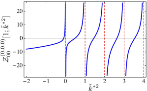
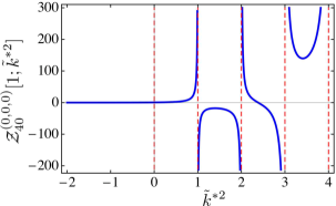
Figure 11: (a) $\mathcal{Z}_{00}^{\mathbf{d}}$ and (b) $\mathcal{Z}_{40}^{\mathbf{d}}$ for $\mathbf{d}=(0,0,0)$ as a function of $\tilde{k}^{*2}=k^{*2}{\rm L}^{2}/4\pi^{2}$.

When $k^{*2}=-\kappa^{2}\leq 0$, the exponential volume dependence of the $c_{LM}^{\mathbf{d}}$ can be made explicit by performing a Poisson resummation of Eq. (3),

$$c^{\mathbf{d}}_{00}(-\kappa^{2};{\rm L})=-\frac{\kappa}{4\pi}+\sum_{\textbf{n}\neq\textbf{0}}{e^{i\pi\textbf{n}\cdot\textbf{d}}}\ \frac{e^{-n\kappa{\rm L}}}{4\pi n{\rm L}}\ \ \ ,$$ (169)

$$c^{\mathbf{d}}_{20}(-\kappa^{2};{\rm L})=-\kappa^{2}\sqrt{4\pi}\sum_{\textbf{n}\neq\textbf{0}}{e^{i\pi\textbf{n}\cdot\textbf{d}}}\ Y_{20}(\hat{\mathbf{n}})\left(1+\frac{3}{n\kappa{\rm L}}+\frac{3}{n^{2}\kappa^{2}{\rm L}^{2}}\right)\frac{e^{-n\kappa{\rm L}}}{4\pi n{\rm L}}\ \ \ ,$$ (170)

$$c^{\mathbf{d}}_{40(\pm 4)}(-\kappa^{2};{\rm L})=\kappa^{4}\sqrt{4\pi}\sum_{\textbf{n}\neq\textbf{0}}{e^{i\pi\textbf{n}\cdot\textbf{d}}}\ Y_{40(\pm 4)}(\hat{\mathbf{n}})\left(1+\frac{10}{n\kappa{\rm L}}+\frac{45}{n^{2}\kappa^{2}{\rm L}^{2}}+\frac{105}{n^{3}\kappa^{3}{\rm L}^{3}}+\frac{105}{n^{4}\kappa^{4}{\rm L}^{4}}\right)\frac{e^{-n\kappa{\rm L}}}{4\pi n{\rm L}}\ \ \ ,$$ (171)

where $\mathbf{n}$ is an integer triplet and $n=|{\bf n}|$. The expansions of $c_{20}^{\mathbf{d}}$ and $c_{40(\pm 4)}^{\mathbf{d}}$ start at $\sim{1\over{\rm L}}e^{-\kappa{\rm L}}$, while $c_{00}^{\mathbf{d}}$ has a leading term that does not vanish in the infinite-volume limit. It is also evident from these relations that $c_{20}^{\mathbf{d}}$ is non-vanishing only for $\mathbf{d}=(0,0,1)$ and $(1,1,0)$, which gives rise to the $\mathcal{O}(\sin\epsilon_{1})$ contributions to the corresponding QCs given in Sec. II.

Previous works Beane et al. (2006, 2013, 2013); Yamazaki et al. (2012); Borasoy et al. (2007); Lee (2009); Bour et al. (2012); Davoudi and Savage (2011), have proposed extracting the infinite-volume deuteron binding energy from the FV spectra using the S-wave QC expanded around the infinite-volume deuteron pole, $\kappa_{d}^{\infty}$, retaining only a finite number of terms in the expansion of the $c_{LM}^{\mathbf{d}}$. Fig. 12 shows the quantity $\delta\mathcal{Z}^{\mathbf{d}}_{00;\mathbf{n}}\equiv\frac{1}{\mathcal{Z}_{00}^{\mathbf{d}}}(\mathcal{Z}_{00}^{\mathbf{d}}-\mathcal{Z}_{00;\mathbf{n}}^{\mathbf{d}})$ as a function of $\kappa{\rm L}$ for different boosts. $\mathcal{Z}_{00;\mathbf{n}}^{\mathbf{d}}$ denotes the value of the $\mathcal{Z}_{00}$-function when the sum in Eq. (169) is truncated to a maximum shell $\mathbf{n}$. For modest volumes, truncating the $\mathcal{Z}$-functions can lead to large deviations from the exact values.

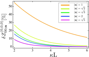
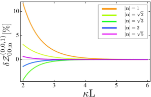
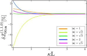
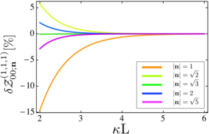
Figure 12: The quantities $\delta\mathcal{Z}^{\mathbf{d}}_{00;\mathbf{n}}\equiv\frac{1}{\mathcal{Z}_{00}^{\mathbf{d}}}(\mathcal{Z}_{00}^{\mathbf{d}}-\mathcal{Z}_{00;\mathbf{n}}^{\mathbf{d}})$ (in percent) as a function of $\kappa{\rm L}$ for different boosts. $\mathcal{Z}_{00;\mathbf{n}}^{\mathbf{d}}$ denotes the value of the $\mathcal{Z}_{00}$-function when the sum in Eq. (169) is truncated to a maximum shell $\mathbf{n}$.

Appendix C Finite-Volume Deuteron Wavefunctions

It is useful to visualize how the deuteron is distorted within a FV, and in this appendix, based on the asymptotic FV wavefunction of the deuteron given in Eq. (25), we show the mass density in the $xz$-plane from selected wavefunctions. As the interior region is not described by the asymptotic form of the wavefunction, it is “masked” by a shaded disk in the following figures. In each figure, the black straight lines separate adjacent lattice volumes that contain the periodic images of the wavefunction.

References

- Beane et al. (2006) S. R. Beane, P. Bedaque, K. Orginos, and M. J. Savage, Phys.Rev.Lett., 97, 012001 (2006), arXiv:hep-lat/0602010 [hep-lat] .
- Ishii et al. (2007) N. Ishii, S. Aoki, and T. Hatsuda, Phys.Rev.Lett., 99, 022001 (2007), arXiv:nucl-th/0611096 [nucl-th] .
- Aoki et al. (2008) S. Aoki, T. Hatsuda, and N. Ishii, Comput.Sci.Dis., 1, 015009 (2008), arXiv:0805.2462 [hep-ph] .
- Beane et al. (2010) S. R. Beane et al. (NPLQCD Collaboration), Phys.Rev., D81, 054505 (2010), arXiv:0912.4243 [hep-lat] .
- Aoki et al. (2010) S. Aoki, T. Hatsuda, and N. Ishii, Prog.Theor.Phys., 123, 89 (2010), arXiv:0909.5585 [hep-lat] .
- Beane et al. (2011) S. R. Beane et al. (NPLQCD Collaboration), Phys.Rev.Lett., 106, 162001 (2011), arXiv:1012.3812 [hep-lat] .
- Beane et al. (2012) S. R. Beane et al. (NPLQCD Collaboration), Phys.Rev., D85, 054511 (2012a), arXiv:1109.2889 [hep-lat] .
- Beane et al. (2012) S. R. Beane, E. Chang, S. Cohen, W. Detmold, H.-W. Lin, et al., Phys.Rev.Lett., 109, 172001 (2012b), arXiv:1204.3606 [hep-lat] .
- Beane et al. (2013) S. R. Beane, E. Chang, S. Cohen, W. Detmold, H.-W. Lin, et al., Phys.Rev., D87, 034506 (2013a), arXiv:1206.5219 [hep-lat] .
- Beane et al. (2013) S. Beane, E. Chang, S. Cohen, W. Detmold, P. Junnarkar, et al., Phys.Rev., C88, 024003 (2013b), arXiv:1301.5790 [hep-lat] .
- Yamazaki et al. (2012) T. Yamazaki, K.-I. Ishikawa, Y. Kuramashi, and A. Ukawa, Phys.Rev., D86, 074514 (2012a), arXiv:1207.4277 [hep-lat] .
- Yamazaki et al. (2012) T. Yamazaki, K.-I. Ishikawa, Y. Kuramashi, and A. Ukawa, PoS, LATTICE2012, 143 (2012b), arXiv:1211.4334 [hep-lat] .
- Murano et al. (2013) K. Murano, N. Ishii, S. Aoki, T. Doi, T. Hatsuda, et al., (2013), arXiv:1305.2293 [hep-lat] .
- Wiringa et al. (1995) R. B. Wiringa, V. Stoks, and R. Schiavilla, Phys.Rev., C51, 38 (1995), arXiv:nucl-th/9408016 [nucl-th] .
- Machleidt (2001) R. Machleidt, Phys.Rev., C63, 024001 (2001), arXiv:nucl-th/0006014 [nucl-th] .
- Bishop and Cheung (1979) D. M. Bishop and L. M. Cheung, Phys. Rev. A, 20, 381 (1979).
- Biedenharn and Blatt (1954) L. C. Biedenharn and J. M. Blatt, Phys. Rev., 93, 1387 (1954).
- Mustafa (1993) M. M. Mustafa, Phys. Rev. C, 47, 473 (1993).
- de Swart et al. (1995) J. de Swart, C. Terheggen, and V. Stoks, (1995), arXiv:nucl-th/9509032 [nucl-th] .
- Luscher (1986) M. Luscher, Commun.Math.Phys., 105, 153 (1986).
- Luscher (1991) M. Luscher, Nucl.Phys., B354, 531 (1991).
- Beane et al. (2004) S. R. Beane, P. F. Bedaque, A. Parreno, and M. J. Savage, Phys.Lett., B585, 106 (2004), arXiv:hep-lat/0312004 [hep-lat] .
- Koenig et al. (2011) S. Koenig, D. Lee, and H.-W. Hammer, Phys.Rev.Lett., 107, 112001 (2011), arXiv:1103.4468 [hep-lat] .
- Bour et al. (2011) S. Bour, S. Koenig, D. Lee, H.-W. Hammer, and U.-G. Meissner, Phys.Rev., D84, 091503 (2011), arXiv:1107.1272 [nucl-th] .
- Davoudi and Savage (2011) Z. Davoudi and M. J. Savage, Phys.Rev., D84, 114502 (2011), arXiv:1108.5371 [hep-lat] .
- Lee (2009) D. Lee, Prog.Part.Nucl.Phys., 63, 117 (2009), arXiv:0804.3501 [nucl-th] .
- Bour et al. (2012) S. Bour, H.-W. Hammer, D. Lee, and U.-G. Meissner, Phys.Rev., C86, 034003 (2012), arXiv:1206.1765 [nucl-th] .
- Detmold and Savage (2004) W. Detmold and M. J. Savage, Nucl.Phys., A743, 170 (2004), arXiv:hep-lat/0403005 [hep-lat] .
- He et al. (2005) S. He, X. Feng, and C. Liu, JHEP, 0507, 011 (2005), arXiv:hep-lat/0504019 [hep-lat] .
- Liu et al. (2006) C. Liu, X. Feng, and S. He, Int.J.Mod.Phys., A21, 847 (2006), arXiv:hep-lat/0508022 [hep-lat] .
- Bernard et al. (2008) V. Bernard, M. Lage, U.-G. Meissner, and A. Rusetsky, JHEP, 0808, 024 (2008), arXiv:0806.4495 [hep-lat] .
- Lage et al. (2009) M. Lage, U.-G. Meissner, and A. Rusetsky, Phys.Lett., B681, 439 (2009), arXiv:0905.0069 [hep-lat] .
- Bernard et al. (2011) V. Bernard, M. Lage, U.-G. Meissner, and A. Rusetsky, JHEP, 1101, 019 (2011), arXiv:1010.6018 [hep-lat] .
- Ishizuka (2009) N. Ishizuka, PoS, LAT2009, 119 (2009), arXiv:0910.2772 [hep-lat] .
- Briceno and Davoudi (2012) R. A. Briceno and Z. Davoudi, (2012), arXiv:1204.1110 [hep-lat] .
- Hansen and Sharpe (2012) M. T. Hansen and S. R. Sharpe, Phys.Rev., D86, 016007 (2012), arXiv:1204.0826 [hep-lat] .
- Guo et al. (2013) P. Guo, J. Dudek, R. Edwards, and A. P. Szczepaniak, Phys.Rev., D88, 014501 (2013), arXiv:1211.0929 [hep-lat] .
- Li and Liu (2013) N. Li and C. Liu, Phys.Rev., D87, 014502 (2013), arXiv:1209.2201 [hep-lat] .
- (39) R. A. Briceno, Z. Davoudi, and T. C. Luu, doi:10.1103/PhysRevD.88.034502.
- (40) http://nn-online.org, Nijmegen Phase Shift Analysis.
- Rummukainen and Gottlieb (1995) K. Rummukainen and S. A. Gottlieb, Nucl. Phys., B450, 397 (1995), arXiv:hep-lat/9503028 .
- Christ et al. (2005) N. H. Christ, C. Kim, and T. Yamazaki, Phys.Rev., D72, 114506 (2005), arXiv:hep-lat/0507009 [hep-lat] .
- Kim et al. (2005) C. Kim, C. Sachrajda, and S. R. Sharpe, Nucl.Phys., B727, 218 (2005), arXiv:hep-lat/0507006 [hep-lat] .
- Blatt and Biedenharn (1952) J. M. Blatt and L. Biedenharn, Phys.Rev., 86, 399 (1952).
- Stoks et al. (1993) V. G. J. Stoks, R. A. M. Klomp, M. C. M. Rentmeester, and J. J. de Swart, Phys. Rev. C, 48, 792 (1993).
- Stoks et al. (1994) V. G. J. Stoks, R. A. M. Klomp, C. P. F. Terheggen, and J. J. de Swart, Phys. Rev. C, 49, 2950 (1994).
- Rijken and Stoks (1996) T. A. Rijken and V. G. J. Stoks, Phys. Rev. C, 54, 2851 (1996a).
- Rijken and Stoks (1996) T. A. Rijken and V. G. J. Stoks, Phys. Rev. C, 54, 2869 (1996b).
- Stapp et al. (1957) H. Stapp, T. Ypsilantis, and N. Metropolis, Phys.Rev., 105, 302 (1957).
- Feng et al. (2004) X. Feng, X. Li, and C. Liu, Phys.Rev., D70, 014505 (2004), arXiv:hep-lat/0404001 [hep-lat] .
- Dresselhaus et al. (2008) M. S. Dresselhaus, G. Dresselhaus, and A. Jorio, Applications of Group Theory to the Physics of Solids, 1st ed. (Springer, 2008).
- Berkowitz et al. (2012) E. Berkowitz, T. D. Cohen, and P. Jefferson, (2012), arXiv:1211.2261 [hep-lat] .
- Oset (2013) E. Oset, Eur.Phys.J., A49, 32 (2013), arXiv:1211.3985 [hep-lat] .
- Sato and Bedaque (2007) I. Sato and P. F. Bedaque, Phys.Rev., D76, 034502 (2007), arXiv:hep-lat/0702021 [HEP-LAT] .
- Bethe (1949) H. A. Bethe, Phys. Rev., 76, 38 (1949).
- Bethe and Longmire (1950) H. A. Bethe and C. Longmire, Phys. Rev., 77, 647 (1950).
- Meyer (2012) H. B. Meyer, (2012), arXiv:1202.6675 [hep-lat] .
- Luu and Savage (2011) T. Luu and M. J. Savage, Phys.Rev., D83, 114508 (2011), arXiv:1101.3347 [hep-lat] .
- Borasoy et al. (2007) B. Borasoy, E. Epelbaum, H. Krebs, D. Lee, and U.-G. Meissner, Eur.Phys.J., A31, 105 (2007), arXiv:nucl-th/0611087 [nucl-th] .