Self-healing Dynamics of Surfactant Coatings on Thin Viscous Films

Abstract

We investigate the dynamics of an insoluble surfactant on the surface of a thin viscous fluid spreading inward to fill a surfactant-free region. During the initial stages of surfactant self-healing, Marangoni forces drive an axisymmetric ridge inward to coalesce into a growing central distension; this is unlike outward spreading, in which the ridge only decays. In later dynamics, the distension slowly decays and the surfactant concentration equilibrates. We present results from experiments in which we simultaneously measure the surfactant concentration (using fluorescently-tagged lipids) and the fluid height profile (via laser profilometry). We compare the results to simulations of a mathematical model using parameters from our experiments. For surfactant concentrations close to but below the critical monolayer concentration, we observe agreement between the height profiles in the numerical simulations and the experiment, but disagreement in the surfactant distribution. In experiments at lower concentrations, the surfactant spreading and formation of a Marangoni ridge are no longer present, and a persistent lipid-free region remains. This observation, which is not captured by the simulations, has undesirable implications for applications where uniform coverage is advantageous. Finally, we probe the generality of the effect, and find that distensions of similar size are produced independent of initial fluid thickness, size of initial clean region, and surfactant type.

I Introduction

Scientists have been intrigued by the spreading of surfactants for centuries: Benjamin Franklin famously wrote of sailors applying oil to the sea in order to “calm the waters” (Franklin et al., 1774). Quantitative experiments began with the work of Agnes Pockels, whose letter to Lord Rayleigh was published in Nature (Rayleigh and Pockels, 1891) and describes the effect of kitchen powders on surface tension. The techniques developed in their early work are alive today (Kaganer et al., 1999) in the form of Langmuir-Blodgett troughs used to study molecular monolayers on fluid surfaces. Studies of surface tension driven spreading began first on deep fluid layers (Hoult, 1972), but in more recent decades, thin fluid films have been recognized as underlying many complex biological and engineering processes. Applications include pulmonary drug delivery (Gaver and Grotberg, 1990) and surfactant replacement therapy (Gaver and Grotberg, 1992), ocular surfactants and blinking dynamics (Braun, 2012; Maki et al., 2010), solute transport (Jensen et al., 1994), latex paint drying (Evans et al., 2000; Gundabala et al., 2008; Gundabala and Routh, 2006), ink-jet printing (Hanyak et al., 2011), and secondary oil recovery (Hanyak et al., 2012; Sinz et al., 2011). In each of these processes, amphiphilic surfactant molecules relax the intermolecular bonds at the surface of an underlying fluid and locally reduce the free energy. Gradients in the concentration of insoluble surfactants cause gradients in the free energy, known as Marangoni forces. These forces provide surface stresses that induce motion in the fluid and in turn advect the surfactant. In the ideal case, spreading results in a homogeneous surfactant distribution, often the desired outcome for medical and engineering applications.

The spreading dynamics of surfactants on thin liquid films are known to depend on both the chemistry of the materials and the geometry of the system. In many cases, the choice of an insoluble surfactant simplifies the dynamics, since for low concentrations the transport of the surfactant molecules is therefore confined to the surface of the fluid (Craster and Matar, 2007). A classic model by Gaver and Grotberg (1990) has long been used to predict the dynamics of the fluid height profile and surfactant distribution for an insoluble surfactant spreading on a thin fluid film. The model is based on the incompressible Navier-Stokes equations, free surface and no slip boundary conditions, and lubrication theory. While theoretical treatments of the subject (Jensen and Grotberg, 1992; Gaver and Grotberg, 1992; Espinosa et al., 1993; Levy and Shearer, 2006) have advanced our understanding, quantitative comparisons between theory and experiments have only recently begun. In particular, predictions for the evolving thickness of the fluid layer have been experimentally tested in both planar and droplet geometries (Gaver and Grotberg, 1992; Dussaud and Troian, 1998; Dussaud et al., 2005; Fallest et al., 2010; Hanyak et al., 2012), but much less is known about the quantitative dynamics of the surfactant concentration (Bull et al., 1999; Fallest et al., 2010; Swanson et al., 2013).

Two geometric properties, aspect ratio and interface curvature, are known to play important roles in spreading dynamics. Surfactants spreading on fluid layers which are thin enough to dewet are known to undergo fingering instabilities Troian et al. (1989); Hamraoui et al. (2004) that are not present when the fluid substrate is thick enough to remain intact. Furthermore, the spreading of circular droplets on thin films (Dussaud et al., 2005; Fallest et al., 2010; Bull et al., 1999; Swanson et al., 2013) exhibit dynamics well-described by a radius which grows as $r(t)\propto t^{1/4}$, while for thicker (non-lubrication) films the growth rate is $r(t)\propto t^{3/4}$. Curvature also affects the spreading rate; for thin fluid films, a planar front spreads as $x(t)\propto t^{1/3}$ (Hanyak et al., 2012), while the aforementioned droplets spread outward at a rate of $r(t)\propto t^{1/4}$ (Fallest et al., 2010; Jensen and Grotberg, 1992; Dussaud et al., 2005; Swanson et al., 2013).

Astonishingly, a third possibility – the spreading of a surfactant into a depleted region – has received comparably little attention. Understanding more about the dynamics in this geometry can shed light on the interactions between disconnected or heterogeneous regions of surfactant coverage as well as the extent to which imperfectly-covered surfaces can self-heal. Prior work by Jensen (1994) analytically solved the model of Gaver and Grotberg (1990) using similarity solutions to understand the dynamics leading up to the closure of the region at time $t_{c}$; the region is predicted to shrink as $r(t)\propto(t_{c}-t)^{0.81}$. From a mathematical standpoint, this “inward” (or hole-closing) geometry qualitatively differs from “outward” and planar spreading in that the area to be covered by surfactant is finite in first case and can be infinite in the later two.

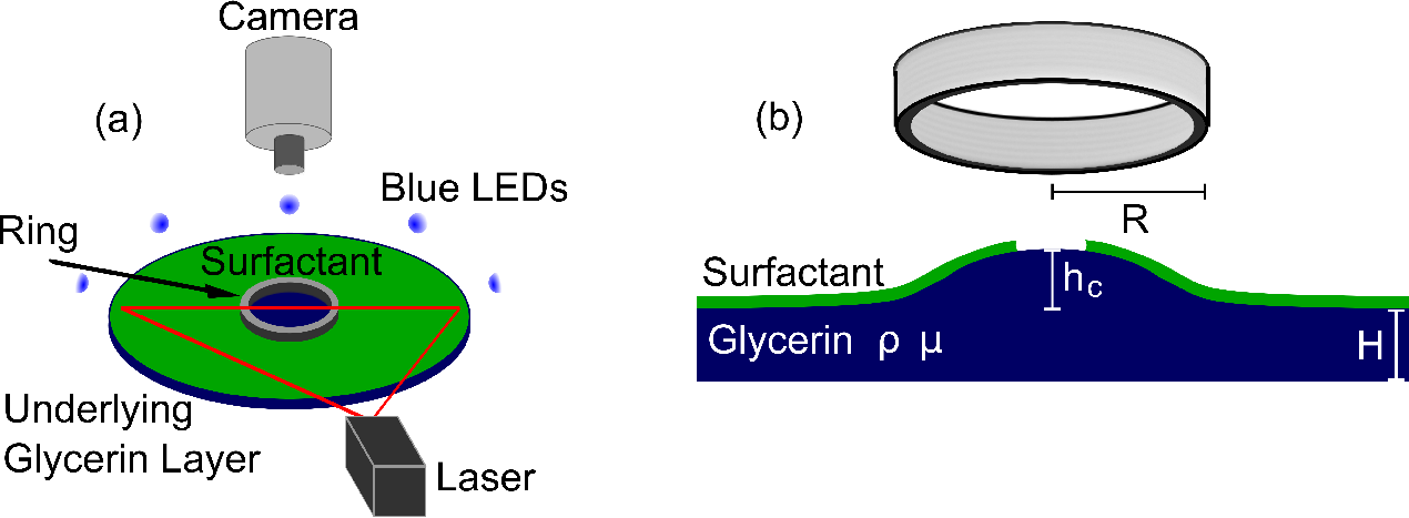
Figure 1: [Color Online] Experiment schematic ($a$) experiment before the barrier ring is lifted. ($b$) cross section of the fluid and surfactant film after the barrier ring is lifted.

In this paper, we address the inward spreading of surfactant into a previously surfactant-free region using both experiment and modeling approaches, as illustrated in Fig. 1. We consider an initially flat fluid film partially covered with surfactant; a circular region of radius $R$ is kept free of surfactant while the area outside this region is coated with a uniform concentration of surfactant $\Gamma_{0}$. The initial fluid film thickness, $H$, is millimetric, and is therefore small compared with the several-centimeter masked region (lubrication theory applies). Using this geometry, we examine the self-healing behavior of these regions, quantify the dynamics, and examine to what extent the model by Gaver and Grotberg (1990) is able to capture these behaviors.

For experiments and simulations performed under matched conditions, we report the evolution of the height profile and surfactant concentration profile as the surfactant spreads inward. Interestingly, we observe that Marangoni forces initially drive fluid into the central region, creating a distension which is also millimetric in scale. By tracking the height of this distension, we are able to separate the dynamics into a growth phase and a decay phase, and examine the dependence of the maximum distension height on both geometric and material parameters of the system. In addition, we simultaneously visualize the advancing front of surfactant by using fluorescently-tagged lipids as the surfactant (Fallest et al., 2010). For large initial surfactant concentrations (approaching a monolayer in coverage), the predicted and observed height profiles agree and the spreading exponent associated with the leading edge of the surfactant matches predictions from the self-similarity analysis of Jensen (1994). However, the dynamics are approximately 10 times faster in the experiments than in the simulations under the assumption that the glycerin is pure (anhydrous). The leading edge is also much sharper in the experiments than in the simulations. Finally, we observe that for initial surfactant concentrations well below a monolayer in coverage, the hole does not completely heal on experimental timescales. We close with a discussion of possible ways to reconcile the observed differences.

II Methods

Using both experiments and simulations, we consider a thin fluid upon which a surfactant spreads from an annular contaminated region into an initially surfactant-free circular central region. This axisymmetric geometry is shown schematically in Fig. 1. Because the classic mathematical model (Gaver and Grotberg, 1990) for surfactant spreading on a thin film makes predictions for both the height profile $h(r,\theta,t)$ of the fluid film and the surfactant concentration $\Gamma(r,\theta,t)$ on its surface, we have designed and built an experimental apparatus which provides access to both dynamics. Below, we describe the experimental methods and materials, as well as the techniques for numerically solving the model in this geometry.

II.1 Experiments

The main apparatus consists of an aluminum well with radius $r_{\mathrm{well}}$ (either 11.1 cm or 14.6 cm) containing a millimetric layer of glycerin. In each experiment, we place an initial concentration of surfactant $\Gamma_{0}$ in the region outside of a cylindrical stainless-steel retaining ring, and this surfactant spreads inward after the ring is lifted out of the fluid. The protocol is geometrically inverted from that used in prior experiments on outward spreading Bull et al. (1999); Gaver and Grotberg (1992); Fallest et al. (2010). We use two measurement techniques to capture the dynamics of this process: laser profilometry (LP), which measures the height profile of the fluid surface, and fluorescence imaging (FI), which records the spatial distribution of fluorescently-tagged surfactants. Using the LP technique, we examine a broad range of surfactants (polydimethylsiloxane, Triton X-305, sodium dodecyl sulfate, oleic acid, and NBD-PC (1-palmitoyl-2-12-[(7-nitro-2-1,3-benzoxadiazol-4-yl)amino]dodecanoyl -sn-glycero-3-phosphocholine)) at bulk volumes in which the surfactant is no longer confined to a monolayer. Using both FI and LP techniques, we examine a fluorescently-tagged phosphocholine lipid (NBD-PC) at monolayer concentrations. The material properties of the five surfactants are provided in Table 1.

The glycerin (Sigma-Aldrich) is initially $\geq 99.5\%$ anhydrous; at $20$ ^∘C, viscosity $\nu=14.1$ Poise Segur and Oberstar (1951), density $\rho=1.26$ g/cm³ Bosart and Snoddy (1928), and surface tension $\sigma_{0}=63$ dynes/cm Gallant (1967). Because glycerin is both hygroscopic and temperature sensitive, the ambient temperature and humidity, which ranged from $(22.8\pm 0.4)^{\circ}$C and $19\%-50\%$ respectively, can affect these physical parameters. In addition, it is possible that chloroform used during surfactant deposition might dissolve in the glycerin and decrease its viscosity. Simply considering hygroscopic effects, the material parameters could range as far as viscosity $\nu=0.45$ Poise Segur and Oberstar (1951), density $\rho=1.20$ g/cm³ Bosart and Snoddy (1928), and surface tension $\sigma_{0}=65$ dynes/cm Gallant (1967). Of these, viscosity is the most significant effect, and its decrease would also cause the timescale of the dynamics to decrease (faster dynamics). In §II.2, we will introduce a parameter $\alpha$ to empirically correct the redimensionalization in order to compare the simulations to the experiments, since the viscosity is unknown.

Surfactant	Surface Tension	Solubility	Solution	$\Gamma_{c}$ $\frac{\mu g}{cm^{2}}$
	$\sigma_{s}$ (dyne/cm)	in glycerin
NBD-PC (Bull et al., 1999; Fallest et al., 2010)	35.5	insoluble	1 $\mu$g of NBD-PC per	0.3
			$\mu$L solution in chloroform
PDMS	20.5	slightly soluble	pure	–
Triton X-305	49	soluble	1% in water	–
SDS (Mysels, 1986)	46	soluble	6 mM in water	–
oleic acid (Gaver and Grotberg, 1992)	32.79	insoluble	0.1% in hexane	0.20

Table 1: Physical and chemical properties of the surfactants and surfactant solutions. For NBD-PC and oleic acid, the value of $\sigma_{s}$ corresponds to the surface tension at or above $\Gamma_{c}$; at $\Gamma<\Gamma_{c}$, the surface tension is higher. For all other materials, $\sigma_{s}$ is the surface tension of the surfactant (or surfactant solution). Data for PDMS and Triton X-305 were obtained from the manufacturer (Shin-Etsu and Dow Chemical, respectively).

	Well,	$R$ (cm)	$H$ (mm)	Surfactant	$\Gamma_{0}$ ($\Gamma_{c}$)	$V$ ($\mu$L)
Technique	Base	$\pm 0.04$ cm	$\pm 0.05$ mm		$\pm 5\%$
FI & LP1	Si	3.0	0.7	NBD-PC	0.2, 0.4, 0.6, 0.8, 1	38.5,77,115.5,154,192.5
LP2	Al	1.5	1.7, 2.0, 2.5, 3.0, 4.0, 5.0	PDMS	–	$540$
LP2	Al	0.8, 1.5, 3.0	2	PDMS	–	$540$
		1.5	2	Triton X-305	–	540
		1.5	2	SDS	–	540
LP2	Al	1.5	2	oleic acid	22	540
		1.5	2	NBD-PC	4.66	540
		1.5	2	PDMS	–	540

Table 2: Summary of experiments (all rows). Simulations were performed with the parameters in the first row. Experiments with fluorescence imaging (FI) use a silicon wafer (Si) to line the bottom of the 14.6 cm radius aluminum well. Experiments which only use laser profilometry (LP) use an anodized 11.1 cm radius aluminum well (Al). Both lasers are from LaserGlow, with a 250 $\mu$m beam thickness; laser 1 is $20$ mW, $532$ nm, fan angle $100^{\circ}$; laser 2 is $5$ mW, $635$ nm, fan angle $30^{\circ}$. Initial concentration $\Gamma_{0}$ is not applicable for soluble surfactants. The volumes reported for NBD-PC and oleic acid are that of the surfactant-solvent solution (see Table 1); the volatile solvent evaporates before the experiment begins. §III.1 and §III.2 report dynamics from only the FI & LP1 experiments; measurements of the distension size are reported for all 5 types of experiments in §III.3.

Each experiment consists of choosing a particular geometry (retaining ring radius $R$ and initial glycerin thickness $H$), and a volume $V$ of solvent-dispersed surfactant deposited outside the retaining ring on the surface of the glycerin. These initial conditions are summarized in Table 2, forming four sets of controlled experiments. It is helpful to consider several dimensionless quantities which characterize the experiments; we calculate these based on anhydrous glycerin at $20$ ^∘C. The Reynolds number $SH^{3}\rho/\nu^{2}R^{2}$ (where $S\equiv\sigma_{0}-\sigma_{s}$ is the maximum reduction in surface tension due to the presence of a particular surfactant) is ${\cal O}(10^{-5})$. The Péclet number $SH/\nu D$ expresses the relative importance of advection with respect to diffusion. The surfactant diffusivity $D$ of similar surfactants has been reported in the literature to be as low as $10^{-10}$ cm²/s and as high as $10^{-4}$ cm²/s (Agrawal and Neuman, 1988). As a conservative estimate, we take the highest value $D=10^{-4}$ cm²/s (Sakata and Berg, 1969), for which the Péclet number is ${\cal O}(10^{3})$. The Bond number $\rho gR^{2}/\sigma_{0}$, which expresses the relative importance of gravitational forces with respect to capillary forces, is ${\cal O}(10^{2})$. The Ohnesorge number $\sqrt{\nu^{2}/\rho SR}$, which expresses the relative importance of viscous stresses with respect to Marangoni stresses, is ${\cal O}(1)$. The Galilei number $\rho^{2}gH^{2}R/\nu^{2}$, which expresses the relative importance of gravitational forces with respect to viscous stresses, is ${\cal O}(10^{-1})$.

Two of the surfactants (NBD-PC and oleic acid) are deposited in solution with a solvent (chloroform) that quickly evaporates. This technique allows us to achieve uniform surfactant concentrations near or below the critical monolayer concentration $\Gamma_{c}$. For these surfactants, we can calculate the initial surfactant concentration $\Gamma_{0}=\frac{VC}{A}$ where $C$ is the mass of surfactant per unit volume solution and $A$ is the surface area initially covered by surfactant ($A=\pi(r_{\mathrm{well}}^{2}-R^{2})$). We usually express $\Gamma_{0}$ as a fraction of $\Gamma_{c}$ and achieve different values of $\Gamma_{0}$ by depositing different volumes of the solvent-dispersed surfactant solution $V$.

Experiments involving surface tension are quite sensitive to the preparation protocol. Therefore, we initially clean all parts using a chemically-appropriate method: detergent (aluminum well), Contrad 70 (glass syringe, stainless-steel retaining ring), and oxygen plasma (silicon wafer). As a final step, we rinse all parts with 18.2 M$\Omega$ deionized water and dry with nitrogen gas. In each experiment, we fill the well with glycerin measured in a glass syringe, and allow the fluid to settle for 2 hours to reach a flat state. The retaining ring is lowered by a nylon line until it just touches the surface of the glycerin, thus dividing the fluid surface into an inner and outer region. With a micro-pipette, we deposit the surfactant (or surfactant solution) in multiple drops in the outer region. A waiting period of 30 min (NBD-PC) or 6 min (all others) is sufficient to allow the spatial distribution to homogenize and the solvent to evaporate for all but the lowest concentration. For the NBD-PC experiments, the initial conditions are readily described by the concentration $\Gamma_{0}$, reported as a fraction of the critical monolayer concentration $\Gamma_{c}=0.3\frac{\mu\mathrm{g}}{\mathrm{cm}^{2}}$ (Bull et al., 1999; Fallest et al., 2010). In the case of the bulk surfactants, the values of $\Gamma_{0}$ are above $\Gamma_{c}$ but this value is nonetheless provided for comparison. Finally, the ring is lifted by a motor at a rate of $100\,\mu$m/s. The partially wet stainless-steel ring, while being lifted, draws up a meniscus of glycerin. Observations begin when the ring separates from the meniscus and is removed from the field of view. A visual inspection of the ring after it detaches reveals a barely-visible layer of glycerin on the bottom of the ring. The main influence of the wettability of the ring is to set the size of the meniscus; the possible effects of this meniscus will be discussed below.

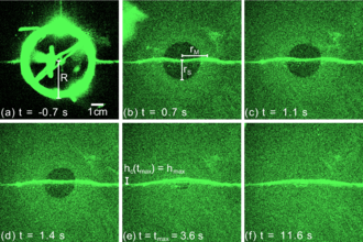
Figure 2: [Color Online] Self-healing of surfactant layer. Sample fluorescence imaging (FI) and laser profilometry (LP) images for $\Gamma_{0}=0.8\Gamma_{c}$, $H=0.7$ mm, and $R=3$ cm. The bright horizontal laser sheet reflection measures the height profile $h(r,t)$, and the background intensity measures the surfactant concentration $\Gamma(r,t)$. The time series of a typical experiment starts when the retaining ring is lifted ($a$), after which the capillary ridge travels inward and forms the vertical distension as the central surfactant-free (dark) region shrinks ($b-d$). At time $t_{\mathrm{max}}$, the distension reaches its largest size ($e$) and then decays ($f$). The position of the maximum of the Marangoni ridge is denoted by $r_{M}$ and the position of the leading edge of the surfactant is denoted by $r_{S}$.

To measure the height profile $h(r,t)$ of the glycerin fluid layer, we use laser profilometry (LP). The setup consists of a laser sheet generator centered along the diameter of the ring, with an incident angle $\approx 20^{\circ}$. When the fluid surface is deformed, the laser sheet is deflected by an amount proportional to the change in the fluid thickness. A camera, positioned directly above the experiment, records the reflection of the laser sheet due to both the top and bottom glycerin interfaces. In the experiments in which the aluminum well serves as the bottom interface, the rough surface causes both reflections to appear as a single profile. In the experiments in which a 8” silicon wafer serves as the bottom interface (the FI/LP experiments), profiles from multiple reflections are visible; an example time series is shown in Fig. 2. We calibrate the proportionality of the deflection and the fluid height using flat glycerin layers of known thickness. To interpret the profile from the raw images, we trace the center of the single profile (LP data set), or the top edge of the uppermost (thinnest) profile (FI/LP data sets). Each column provides a single value in $h(r)$ to within one pixel ($0.037$ mm); individual columns (and, infrequently, images) are rejected from the data set if they are statistical outliers arising from image imperfections.

To measure the surfactant concentration profile $\Gamma(r,t)$ in experiments using NBD-PC surfactant, we use fluorescence imaging (FI). In experiments where we use this technique, the basic apparatus is modified in several ways. Eight blue LEDs (1.5 W, $467$ nm from Visual Communications Company, Inc.) are arranged in an evenly spaced circle around the edge of the aluminum well so that direct rays of light are reflected away from the camera by the silicon wafer placed in the bottom of the aluminum well. These LEDs are close to the $464$ nm absorption peak of the NBD fluorophore. Imaging is performed with a cooled $14-$bit Andor Luca$-$R camera with $1004\times 1002$ resolution. The camera is fitted with a Newport bandpass filter at $(530\pm 10)$ nm to preferentially collect photons emitted near the $531$ nm emission peak of the NBD fluorophore. The exposure time for each image is $1/4$ s with a frame rate of $2-3$ Hz, which allows for a high enough signal-to-noise ratio to image concentrations down to $\lesssim 0.05\Gamma_{c}$.

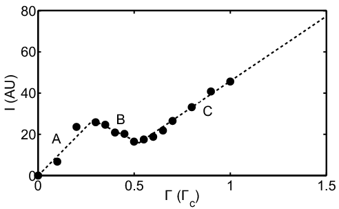
Figure 3: Calibration data relating surfactant concentration $\Gamma$ to fluorescence intensity $I$. Because the curve is non-monotonic, we use a piecewise linear fit (regions A, B, C) to the empirical data. Error bars (standard deviation of the mean intensity) are smaller than the points.

We calibrate the relationship between image intensity and surfactant concentration $\Gamma$ by depositing a known concentration of NBD-PC on a flat glycerin surface and recording the average brightness within a $10\times 10$ cm² region at the center of the image. At the lowest concentrations, ($<0.3\Gamma_{c}$), the surfactant remains inhomogeneously distributed despite waiting 2 hours after deposition. For these experiments, we illuminate the experiment with only the blue LEDs. In addition, the calibration accounts for a temperature-dependent offset value which is manifest as a slow drift in the average image intensity. As is expected for molecular fluorescence, the relationship is non-monotonic due to fluorescence resonance energy transfer (FRET) effects Shrive et al. (1995). The resulting calibration is shown in Fig. 3.

To calculate $\Gamma(r)$ from the images, we first crop and threshold the image to remove imperfections, and mask the region containing the laser profile. As a consequence, we do not report FI data for the central $8$ mm of the image. Using the remaining values, we azimuthally average the image intensity in 2 pixel wide bins. To account for the slow temperature drift, we set $\Gamma\approx\Gamma_{0}$ for large $r$ and, if needed, $\Gamma\approx 0$ at the center. Because $I(\Gamma)$ is non-monotonic, we must develop an inversion procedure to measure $\Gamma(I(r))$. We start from a piecewise-linear fit to $I(\Gamma)$ (see Fig. 3), and use a combination of interpolation and continuation methods to perform the inversion. For regions where $\Gamma(I)$ is ambiguous, we assume continuity of $\Gamma(I(r))$ and extrapolate from unambiguous regions by identifying the correct piecewise regime (A, B, C from Fig. 3) to use. This method even works when $I(r)$ crosses through all 3 regimes within a few pixels, as occurs at the leading edge of the inward-spreading surfactant, by relying on extrapolation from both sides. Note that $\Gamma(r)$ curves can rise above the initial $\Gamma_{0}$ value by drawing material from other regions.

II.2 Model

The classic Gaver-Grotberg model Gaver and Grotberg (1990) for the spreading of insoluble surfactant on a thin liquid film is based upon low Reynolds number flow in a small aspect ratio system. Marangoni stresses at the fluid surface drive flow in the bulk. The velocity of the flow is determined by the no-slip boundary condition at the container bottom. The normal and tangential stresses, including gravity (via hydrostatic pressure) and capillarity (via normal surface stress condition), balance at the fluid surface. The resulting system of nonlinear partial differential equations is

$$\tilde{h}_{\tilde{t}}+\nabla\cdot\left(\frac{1}{2}\tilde{h}^{2}\nabla\tilde{\sigma}\right)=\beta\nabla\cdot\left(\frac{1}{3}\tilde{h}^{3}\nabla\tilde{h}\right)-\kappa\nabla\cdot\left(\frac{1}{3}\tilde{h}^{3}\nabla\nabla^{2}\tilde{h}\right)$$ (1)

$$\tilde{\Gamma}_{\tilde{t}}+\nabla\cdot\left(\tilde{h}\tilde{\Gamma}\nabla\tilde{\sigma}\right)=\beta\nabla\cdot\left(\frac{1}{2}\tilde{h}^{2}\tilde{\Gamma}\nabla\tilde{h}\right)-\kappa\nabla\cdot\left(\frac{1}{2}\tilde{h}^{2}\tilde{\Gamma}\nabla\nabla^{2}\tilde{h}\right)+\delta\nabla^{2}\tilde{\Gamma}.$$ (2)

where $\tilde{h}({\bf\tilde{r}},\tilde{t})$ is the fluid height and $\tilde{\Gamma}({\bf\tilde{r}},\tilde{t})$ is the surfactant concentration. For clarity, all non-dimensional variables are denoted with a tilde to distinguish them from their dimensional analogues (e.g. $\tilde{t}$ is a non-dimensional quantity while $t$ has dimensions of seconds). In Eqn. 1, gravity smooths the height profile, driving the surface to be flat while capillarity affects curvature in the fluid surface Peterson (2010). For simplicity, capillarity is assumed to be a property of the fluid and independent of the surfactant-fluid interaction. The fluid height evolution equation is derived from fluid incompressibility where the convective derivative uses the depth-averaged velocity. The surfactant evolution equation is derived from an advection-diffusion equation in which the surface convective derivative contains the fluid surface velocity and the surfactant diffuses on the surface. The diffusion smooths the surfactant profile, slowly causing the surfactant to reach a uniform coverage independent of Marangoni stresses. In both equations, the $\nabla\tilde{\sigma}$ term ($\nabla=\partial_{\tilde{x}}\hat{x}+\partial_{\tilde{y}}\hat{y}$) describes the effect of gradients in surfactant concentration.

The relationship between surface tension and surfactant concentration is provided by an equation of state. We use

$$\tilde{\sigma}(\tilde{\Gamma})=\left(1+\eta\tilde{\Gamma}\right)^{-3},$$ (3)

(see Fig. 4) which was proposed by Borgas and Grotberg (2006) as an alternative to the linear equation of state because it can model concentrations beyond a monolayer of surfactant Swanson et al. (2013). Empirical measurements of the equation of state of lipids typically have a regime where the surface tension remains constant for concentrations greater than $\Gamma_{c}$, above which the monolayer becomes sufficiently close-packed that no additional molecules can fit on the fluid surface (Kaganer et al., 1999). For $\Gamma>\Gamma_{c}$, three-dimensional structures are created, but because surfactant molecules only lower the surface tension when they are in contact with the surface, the surface tension does not change further. In Eqn. 3, the material parameter $\eta\equiv\frac{\sigma_{s}}{\sigma_{0}-\sigma_{s}}$ is determined from both the surface tension $\sigma_{0}$ of the surfactant-free glycerin and that of the surfactant-contaminated fluid ($\sigma_{s}$) when $\Gamma=\Gamma_{c}$. Based on material parameters for NBD-PC on glycerin, we choose $\eta=1.2562$. For the NBD-PC experiments, $\sigma_{s}$ is set by the empirically-determined minimum surface tension Bull et al. (1999) which is reached at or above the critical monolayer concentration, $\Gamma_{c}$. For a monolayer of molecules, this molecular thickness is a negligible contribution to $\tilde{h}(\tilde{r})$.

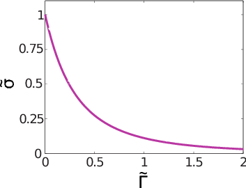
Figure 4: The equation of state used in the simulations (Eqn. 3). The equation of state relates the nondimensional surface tension $\tilde{\sigma}$ to the nondimensional surfactant concentration $\tilde{\Gamma}$.

There are three non-dimensionalized coefficients in the model, each of which controls the magnitude of a particular term. The second-order $\beta$ terms incorporate the effect of gravity, while the fourth-order $\kappa$ terms model the effect of capillarity on the system. The surfactant equation also has a $\delta$ term representing surfactant diffusion on the surface of the film. We compute these three coefficients according to

$$\beta\equiv\frac{\rho gH^{2}}{S},\qquad\kappa\equiv\frac{\sigma_{0}H^{2}}{SL^{2}},\qquad\delta\equiv\frac{\nu D}{SH}$$ (4)

using physical values from Table 1 and the dimensions of our experiments. Here, $\rho$ is the fluid density, $\nu$ is the fluid viscosity, $g$ is the acceleration due to gravity, $L$ is the characteristic length (taken to be the ring radius $R$), and $H$ is the characteristic fluid height (taken to be the initial fluid height). The validity of the lubrication approximation, an important assumption of the model, is limited by how thin we can make the glycerin layer before it dewets during surfactant deposition. Our thinnest stable films are $H=0.7$ mm thick. For the largest retaining ring ($R=3$ cm), this provides an aspect ratio of $\epsilon=0.02$. The parameter $S$ is determined by the range of surface tension values accessible to the materials in the system. From the diffusivity ($D=10^{-4}$ cm²/s), we calculate the time scale for purely diffusive self-healing of our monolayer films as $R^{2}/D=10^{4}-10^{5}$ s (2 to 25 hours, depending on the size of the ring). Using these values, together with the parameters in Table 2, we calculate $\beta=2.13612\times 10^{-1}$, $\kappa=1.22839\times 10^{-3}$, and $\delta=7.17844\times 10^{-4}$.

We calculate numerical solutions using an open source numerical solver (Claridge et al., 2013) designed to solve coupled hyperbolic-parabolic nonlinear partial differential equations, such as Eqn. 1 and Eqn. 2. The package employs a finite volume scheme for nonlinear systems of PDEs up to fourth-order without restrictions on boundary conditions, minimizes per-problem code-development, and enables rigorous, automated convergence testing on problems with analytical solutions. We use a rectangular grid so as not to impose a symmetric solution via the solver (Kronmiller et al., 2013), and find that the solutions are axisymmetric. Without loss of generality (and to facilitate direct comparison with the azimuthally averaged experimental data), we present cross-sections of the redimensionalized height and surfactant profiles in the $y=0$ plane (coplanar with $\theta=0$ plane). Additionally, the abscissa of the height and surfactant profile plots in §III is labeled $r$ instead of $\tilde{x}$. The distance between cells is 0.035 dimensionless spatial units; we compute on the domain $[-3.4825,3.4825]$ (in dimensional units: $[-10.4475\,\mathrm{cm},10.4475\,\mathrm{cm}]$) using Dirichlet boundary conditions. Convergence of the solver’s solutions for similar problems has been shown in previous work (Kronmiller et al., 2013; Claridge et al., 2013). We do not consider reflections from the edges of the well, which is appropriate for the inward spreading case.

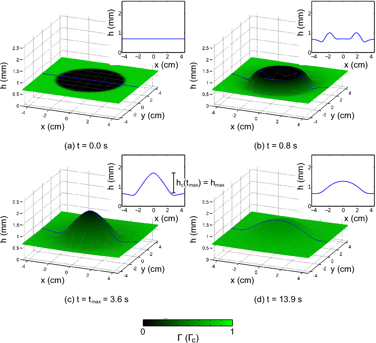
Figure 5: [Color Online] Typical numerical simulations with growth and decay of fluid and self-healing of surfactant. Redimensionalized numerical simulations of Eqn. 1 and Eqn. 2 using $\Gamma_{0}=0.8\Gamma_{c}$, $H=0.7$ mm, and $R=3$ cm (the same parameters as in Fig. 2). In each panel, the surface represents $h(x,y,t)$ and the color of the surface ranges from $\Gamma=0\Gamma_{c}$ (black) to $\Gamma=1\Gamma_{c}$ (green). The insets highlight the shape of $h(y)$ cut through the center of the surface plots. The simulation starts from ($a$) the initial film height and surfactant concentration, and the resulting dynamics are ($b$) the formation of the distension as the annular Marangoni ridge coalesces toward the center of the region. At time $t_{\mathrm{max}}$, the distension reaches its largest size ($c$) and then decays ($d$). Times have been redimensionalized by $T/\alpha_{0.8}$, as will be discussed in §III, to permit a direct comparison with the experiments.

To model the initial condition of the physical experiment, we use a uniform initial film height of $\tilde{h}=1$ and an initial surfactant concentration of

$$\tilde{\Gamma}(\tilde{r};\tilde{t}=0)=\tilde{\Gamma}_{0}\frac{1}{2}\left[1-\tanh\left(20\left(1-\tilde{r}\right)\right)\right],$$ (5)

where $\tilde{r}$ is the radial coordinate. Sample solutions representing the resulting inward-spreading dynamics for NBD-PC are shown in Fig. 5. Each panel represents both $h(r,t)$ and $\Gamma(r,t)$ (redimensionalized for comparison) at the same instant.

When making comparisons between experimental results and numerical solutions of this model, we reintroduce dimensions into the numerical results using $h=\tilde{h}\,H,$ $\Gamma=\tilde{\Gamma}\,\Gamma_{c}$ and $\Gamma_{0}=\tilde{\Gamma}_{0}\,\Gamma_{c}$. The timescale is expected Gaver and Grotberg (1990) to be similarly redimensionalized according to time $t=\tilde{t}\,T$, where

$$T=\frac{\nu L^{2}}{SH}.$$ (6)

However, we observe that the simulated fluid height profile and surfactant distribution both evolve more slowly than the experiment by a factor of approximately 10. This discrepancy in the speed of the dynamics indicates that the redimensionalization timescale is incorrect. One possible explanation is a decrease in the viscosity of the glycerin layer, as described in §II.1. To account for this discrepancy in timescale, we introduce an empirical factor $\alpha$ into the redimensionalization: $t=\tilde{t}\frac{T}{\alpha}$. Effectively, this speeds up the simulations by a factor of $\alpha$. The choice of $\alpha$ will be described in §III, and all simulation results will have the times redimensionalized in this way.

III Results

In both experiments and simulations, we observe a self-healing phenomenon, whereby a surfactant on a contaminated surface spreads inward, covering the initially surfactant-free region. The surfactant-depleted region can persist for several minutes, and the closing process is accompanied by a corresponding rise in the fluid level at the center of the region. In this section, we characterize the dynamics of this process and evaluate the efficacy of the model in capturing the phenomenon. For simplicity, we report all variables in their dimensionalized form.

Because our experiments capture the spatiotemporal evolution of the surfactant concentration profile $\Gamma(r,\theta,t)$ and height profile $h(r,t)$ for different initial concentrations of surfactant, we can compare the simulation results to the experiments outlined in Table 2. To characterize the dynamics of the growth of the distension, we consider $h_{c}(t)$, the height of the distension at the center of the domain, as well as $h_{\mathrm{max}}=h_{c}(t_{\mathrm{max}})$, the maximum height attained. Note that in the FI/LP experiments (and their corresponding simulations), only monolayer concentrations of NBD-PC surfactant are explored, while the LP experiments include bulk surfactants. In the LP experiments, we can nonetheless characterize the dependence of $h_{\mathrm{max}}$ for different initial fluid heights, ring sizes, and types of surfactant. We do not report simulations for the LP (bulk surfactant) experiments, since they are far beyond the monolayer regime and therefore violate the assumptions of the model.

Fig. 2 shows a prototypical inward spreading (FI/LP) experiment, visualized from above. The first image (a) shows the ring before it is lifted; light reflected from the ring obscures the lipid fluorescence. In (b-f) the speckled green outer region indicates the presence of surfactant, and the black central region is initially surfactant-free. The bright green curve through the center of the images is the intersection of the laser sheet with the surface of the fluid, which provides a profile of the fluid height. A simulation using the same material parameters and initial geometry is shown in Fig. 5, where the green shading represents the surfactant concentration, and the blue curve in the insets provide a view analogous to the green laser profile.

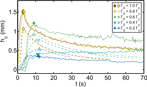
Figure 6: [Color Online] Distension growth and decay. Dynamics are captured by tracking height $h_{c}$ at the center of the system. Experiments (filled symbols) and redimensionalized simulations (open symbols) at five different initial surfactant concentrations. As discussed in §II.2,

simulation times have been redimensionalized and then further reduced by a factor ${\alpha}_{0.2}=17.2{\genfrac{}{}{0.0pt}{}{+12}{-0.0}}$, ${\alpha}_{0.4}=7.81\pm 2$, ${\alpha}_{0.6}=6.07\pm 1$, ${\alpha}_{0.8}=11.0\pm 1$, and ${\alpha}_{1.0}=9.91\pm 2$, respectively, where the $\pm$ values represent the uncertainty in $\alpha$.

In experiments and simulations, similar dynamics are observed. First, a fluid distension forms as the annular Marangoni ridge coalesces in the center of the surfactant-free region. The distension reaches a maximum height $h_{\mathrm{max}}$ at time $t_{\mathrm{max}}$, after which the distension decays. To quantitatively compare experimental data with simulations, we redimensionalize the simulation data as described in §II.2. As illustrated in Fig. 6, we empirically determine the best redimensionalization timescale $T/\alpha$ by comparing the dynamics at the center of the distension, $h_{c}(t)$. For each value of $\Gamma_{0}$, we choose $\alpha$ so that both the rise time and the observed $t_{\mathrm{max}}$ approximately coincide. In all cases, we find that the simulation timescale needs to be decreased by a factor of approximately 10. The resulting $\Gamma_{0}$-dependent values of $\alpha$ are provided in the caption to Fig. 6 and used throughout the remainder of the paper.

Fig. 6 characterizes the dynamics of the distension growth and decay at the center of the system, comparing $h_{c}(t)$ for five different initial surfactant concentrations drawn from the FI/LP experiments. We find that the simulation is able to semi-quantitatively capture a number of key features observed in the experiment, beginning with the observation that the distension is approximately 1 mm high. In both simulations and experiments, we observe that the maximum value of $h_{c}$ increases with surfactant concentration (and thus increased surface tension contrast). This trend will be explored quantitatively in §III.3. In all cases, the growth process is faster than the decay process. In addition, both simulations and experiments show a transition in the sharpness of the growth/decay dynamics ($h_{c}$), with a more pronounced peak present for larger values of $\Gamma_{0}$. Intriguingly, the $1.0$ and $0.8,\Gamma_{c}$ curves are almost coincident with each other in both the experiments and simulations. One key disagreement between experiment in simulations is that for the $1.0,0.8$ and $0.6\,\Gamma_{c}$ experiments, $h_{\mathrm{max}}$ is 0.3 to 0.4 mm taller in the experiments than in the simulations. However, we note that this difference corresponds to the height of the meniscus formed when the ring lifts from the fluid surface. Second, we observe that for experiments starting from $0.2$ and $0.4\,\Gamma_{c}$ initial conditions, the meniscus is large enough to obscure the observation of the distension, whereas in the simulations, the distension is clearly present.

The growth and decay dynamics at higher concentrations can be understood as arising from surface tension gradients. In the growth phase, fluid with higher surface tension (fluid initially surfactant-free inside the ring) pulls the surfactant-rich low surface tension fluid inward. The fluid advects the surfactant and heals (closes) the surfactant layer hole while horizontal gradients in the velocity field result in an annular Marangoni ridge. This ridge moves toward the center, and coalesces into the central distension. In the decay phase, the distension decreases in height until the surface has uniform height while the surfactant concentration homogenizes. In the sections that follow, we quantitatively examine the spatial distributions of surfactant which underlie these dynamics of these two phases.

III.1 Distension Growth

During the growth phase, the motion of the fluid both raises a central distension and advects surfactant inward. In Fig. 7, we show an example ($\Gamma_{0}=0.6\Gamma_{c}$) of the evolution of both $h(r,t)$ and $\Gamma(r,t)$ during the growth of the distension. Here, and also in several plots that follow, the center of the system is at $r=0$, and therefore inward spreading corresponds to motion to the left. In addition, note that at a given time, $\Gamma(r;t)$ represents the concentration of a molecular monolayer, and that the thickness of this layer is many orders of magnitude smaller than $h(r;t)$. In panels $a$ and $b$, we observe that the simulations semi-quantitatively capture the observed dynamics of $h(r,t)$.

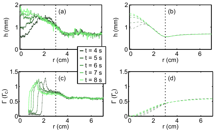
Figure 7: [Color Online] Distension growth dynamics. ($a$,$c$) Experiments (solid) and ($b$,$d$) redimensionalized simulations (dashed) of distension growth dynamics for initial conditions $\Gamma_{0}=0.6\,\Gamma_{c}$, $R=3$ cm, and $H=0.7$ mm. Height profile $h(r,t)$ ($a$,$b$) and surfactant concentration profile $\Gamma(r,t)$ ($c$,$d$) at representative times during growth. Vertical dotted line indicates the initial ring location at $r=R$. Note that gradients in the surface tension field are not significant when $\Gamma>\Gamma_{c}$.

Figure 8: [Color Online] Kymograph of the surfactant concentration profile for the 0.6 $\Gamma_{c}$ experiment. Surfactant propagates outward in the region demarcated by the two white dashed lines. The color scale is truncated at $0.55\Gamma_{c}$ and $0.75\Gamma_{c}$ in order to isolate the region of interest. For reference, the maximum surfactant concentration within the green colored saturated region is $1.4$ $\Gamma_{c}$.

In contrast, we find that the simulated $\Gamma(r,t)$ (panel $d$) takes a quite different shape from what we have observed in experiments (panel $c$); similar disagreement has been found for the case of droplet-spreading (Fallest et al., 2010; Swanson et al., 2013). First, we observe that the experiments exhibit a sharp (1 mm) interface at the leading edge of the advancing front of surfactant (location $r_{S}$). In contrast, the simulations show transition region with a width similar to retaining ring radius $R=3$ cm. Second, we observe a sharp peak in the surfactant concentration directly behind $r_{S}$ not present in the simulations. Visual inspection of the original images suggests that this feature arises from the lift-off of the retaining ring, and it may be that these dynamics cause the formation of a bilayer or other condensed phase (Kaganer et al., 1999). On each side of this peak there is a gradient in $\Gamma$; the opposite signs indicate that the surfactant should spread in both directions. Indeed, we see both the leading edge and the peak travel toward the center of the experiment (self-healing). Simultaneously, the shallower gradient that trails the peak forms an enhanced surfactant plateau that moves outward. This feature is visible in Fig. 8. If this outward propagation of surfactant is advection, then the fluid must bear outward surface currents, an effect absent in the simulation but predictable from the balance of Marangoni stress and viscous shear stress present in lubrication theory. Both features – the peak in $\Gamma$ and the trailing plateau – are notably absent from the simulations. A leading plateau was previously observed in outward-spreading experiments (Fallest et al., 2010; Swanson et al., 2013), and models have so far been unable to capture either feature (Swanson et al., 2013). Its absence is likely due to both a failure to account for surfactant build up on the meniscus and the choice of the equation of state (Eq. 3), which does not account for any condensed phases. Were such structures present, it is possible that they are advected by the underlying fluid velocity. In spite of these difficulties, the simulated $\Gamma(r,t)$ is able to capture surfactant self-healing.

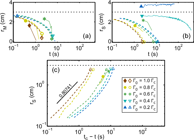
Figure 9: [Color Online] Maragoni ridge and surfactant leading edge dynamics. ($a$) The peak of the Marangoni ridge ($r_{M}$) and ($b$) the inward motion of the leading edge of the surfactant ($r_{S}$) at five different initial surfactant concentrations, for both experiments (solid lines) and redimensionalized simulations (dashed lines). For the experiments, all locations are determined by visual inspection of the $h(r,t)$ and $\Gamma(r,t)$ profiles. In the simulations, $r_{S}$ is the first point where the surfactant concentration rises above $0.001$ $\Gamma_{c}$; choosing a lower threshold does not significantly affect the results. In all cases, $R=3.0$ cm and $H=0.7$ mm; the horizontal dotted line indicates the initial ring location at $r=R$. The closing time $t_{c}$ is defined as time at which $r_{S}=0$; in the experiments, this is found by visual inspection of the images. ($c$) The position of the leading edge of the surfactant (same data as $a$), but plotted as a function of ($t_{c}-t$) to permit comparison to the asymptotic solution from Jensen (1994) (black line). The symbols identify the initial conditions used for each curve.

During the growth phase, we quantify the spreading dynamics by measuring the location of both the peak of the Marangoni ridge ($r_{M}$) and the leading edge of the surfactant ($r_{S}$), with respect to the center at $r=0$. These dynamics are shown in Fig. 9$a$,$b$. No data is shown for $r_{M}$ at $\Gamma_{0}=0.2\,\Gamma_{c}$ and $0.4\,\Gamma_{c}$ because the Marangoni ridge, if present, is obscured by the meniscus. No data is shown for $r_{S}$ at $\Gamma_{0}=1.0\Gamma_{c}$ (and limited data at $\Gamma_{0}=0.8\Gamma_{c}$ and $0.6\Gamma_{c}$) because the dynamics were faster than could be captured by the optics. We observe that $r_{S}$ and $r_{M}$ approximately coincide in all cases, but that self-healing (if it is observed), occurs after the fully-formed distension at $t_{\mathrm{max}}$. An example of these dynamics are shown in Fig. 7 for $\Gamma_{0}=0.6\,\Gamma_{c}$. In all cases except for $\Gamma_{0}=0.2\Gamma_{c}$, we observe that self-healing occurs within $10^{2}$ s (a few minutes), which is far shorter than the diffusive timescale of $10^{5}$ s. Therefore, the self-healing is a Marangoni-driven process. As such, the closing dynamics in both simulations and experiments are faster for larger $\Gamma_{0}$, as would be expected due to the larger surface tension gradients. In simulations, unlike experiments, self-healing always occurs.

Self-healing was predicted by Jensen (1994) to take the asymptotic form $r_{S}(t)\propto(t_{c}-t)^{0.80741}$, where $t_{c}$ is the time at which $r_{S}$ reaches zero and the surfactant-free region is closed. In Fig. 9$c$, we compare this form to our simulations and experiments; note that here time progresses from right to left. The simulations agree as expected because they are solutions of the same equations, but with the $\beta$ and $\kappa$ terms included. For experiments with $\Gamma_{0}=0.6$ or $0.8\,\Gamma_{c}$ (the two experiments with sufficient data available, although less than a decade), we observe approximate agreement with the predicted exponent. Additionally, these figures show that the choice of $\alpha$ for analyzing $t_{\mathrm{max}}$ (based upon fluid height profile data) also yields approximately correct values for $t_{c}$ for the three runs with the highest initial surfactant concentrations. In contrast, $t_{c}$ for the $0.4\,\Gamma_{c}$ experiment is more than an order of magnitude larger than the redimensionalized simulation, and $t_{c}$ for the 0.2 $\Gamma_{c}$ experiment could not be measured. This indicates that a different process controls the timescale at low concentrations.

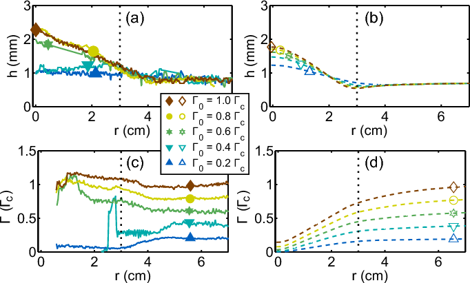
Figure 10: Profiles at $t_{\mathrm{max}}$ for range of $\Gamma_{0}$. ($a$, $b$) Fluid height and ($c$,$d$) surfactant concentration profiles for FI/LP experiments and redimensionalized simulations at time $t_{\mathrm{max}}$, starting from five values of $\Gamma_{0}$ with $R=3.0$ cm and $H=0.7$ mm. ($a$, $c$) Experiments and ($b$,$d$) simulations are plotted in solid and dashed lines respectively. Vertical dotted lines indicate the initial ring location at $r=R$. From lowest to highest $\Gamma_{0}$, $t_{\mathrm{max}}$ is $12.08$, $11.25$, $9.02$, $3.60$, and $3.21$ (s). The symbols identify the initial conditions used for each curve.

The growth phase ends when the distension reaches its maximum height $h_{\mathrm{max}}$ at time $t_{\mathrm{max}}$. In Fig. 10, we compare $h(r,t)$ and $\Gamma(r,t)$ at this time. We observe semi-quantitative agreement in $h(r,t)$ for experiments and simulations, but only for $\Gamma_{0}=0.6,0.8,$ and $1.0\,\Gamma_{c}$. At lower initial concentrations, the formation of a central distension is suppressed only in the experiments. Once again the surfactant concentration profiles $\Gamma(r,t)$ show much less agreement between simulations and experiments. For all runs, the simulations have self-healed ($\Gamma(0)>0.0001\,\Gamma_{c}$) by the time of $t_{\mathrm{max}}$ but retain a strong concentration gradient. In contrast, the experiments self-heal (if at all), after $t_{\mathrm{max}}$.

III.2 Distension Decay

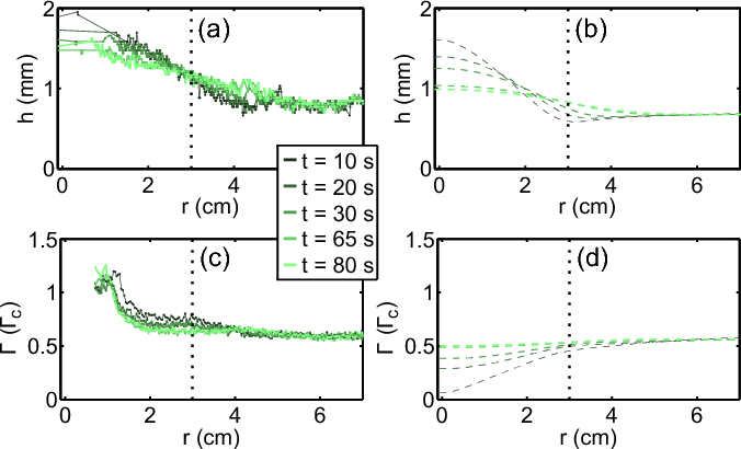
Figure 11: [Color Online] Distension decay dynamics. ($a$,$c$) Experiments (solid) and ($b$,$d$) redimensionalized simulations (dashed) of distension decay dynamics for initial conditions $\Gamma_{0}=0.6\,\Gamma_{c}$, $R=3$ cm, and $H=0.7$ mm. Height profile $h(r,t)$ ($a$,$b$) and surfactant concentration profile $\Gamma(r,t)$ ($c$,$d$) at representative times during decay. Vertical dotted line indicates the initial ring location at $r=R$.

During the decay phase of the distension after $t_{\mathrm{max}}$ the fluid returns from $h_{\mathrm{max}}$ to its original uniform height and $\Gamma(r,t)=const.$ Fig. 11 shows this continuation of the growth dynamics begun in Fig. 7; here, because the dynamics have slowed, we examine profiles at longer intervals of time. Three driving forces are at work in the decay: gravitational forces (decreasing $h_{\mathrm{max}}$), capillary forces (decreasing $h_{\mathrm{max}}$), and Marangoni forces (equilibrating the surfactant distribution and smoothing $\Gamma(r,t)$). In the experiment, the sign of $\nabla\Gamma(r,t)$ indicates that although the surfactant is still being advected inward by the fluid, it is also spreading outward to equilibrate the concentration, as is visible in Fig. 8. Again, while the simulations show reasonable agreement for $h(r,t)$, they fail to capture the observed surfactant concentration profile. In the simulations, the decay dynamics simply involve the inward motion of the surfactant as the concentration gradient relaxes monotonically.

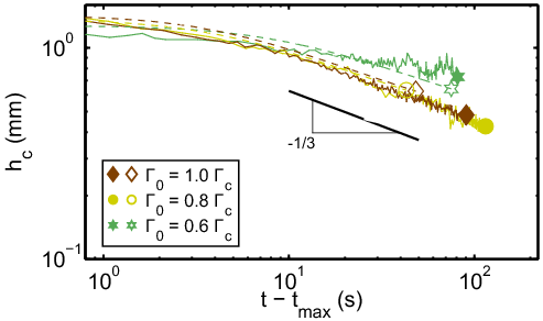
Figure 12: Power law decay near $\Gamma_{c}.$ Comparison of experiments (solid lines) and redimensionalized simulations (dashed lines) at three values of $\Gamma_{0}$, highlighting the distension decay dynamics using data from Fig. 6. The simulations account for the presence of the meniscus by adding the experimentally-observed meniscus height. The solid line is a comparison to a power law decay with exponent $-1/3$, provided for comparison. The symbols identify the initial conditions used for each curve.

To examine the asymptotic behavior of the decay process, we examine the decreasing distension height $h_{c}$ as a function of $t-t_{\mathrm{max}}$. Fig. 12 provides a comparison of these dynamics for experiments and simulations. In order to make a direct comparison, we added the experimentally-observed meniscus height ($0.36$ mm) to all values of $h_{c}$ in the simulations. For $\Gamma_{0}=0.6,0.8,$ and $1.0\,\Gamma_{c}$, we find quantitative agreement between experiments and simulations, in spite of the disagreement in the spatial distribution of surfactant. In the long-time limit, the asymptotic decay dynamics appear to be governed by

$$h_{c}(t)\propto(t-t_{\mathrm{max}})^{-1/3},$$ (7)

with a slightly smaller exponent for $\Gamma_{0}=0.6\,\Gamma_{c}$. We exclude the data for $\Gamma_{0}=0.2$ and $0.4\,\Gamma_{c}$ from this comparison because the height at the center is changing primarily due to the effect of the meniscus (rather than the surfactant).

III.3 Distension Size

In addition to the FI/LP experiments with NBD-PC as the surfactant, we also perform experiments with a variety of other common surfactants, using both monolayer and bulk concentrations. The geometries of these experiments, and the properties of these surfactants are summarized in Tables 1 and 2. To isolate geometric effects which govern the distension height $h_{\mathrm{max}}$, we perform experiments and simulations on a single material while varying ring radius $R$ or fluid depth $H$. Similarly, to isolate material effects, we examine a single geometry (fixed $R$ and $H$) while varying either the surfactant type or its concentration. These experiments lie outside various of the model assumptions: the lubrication approximation, insolubility, and monolayer concentrations.

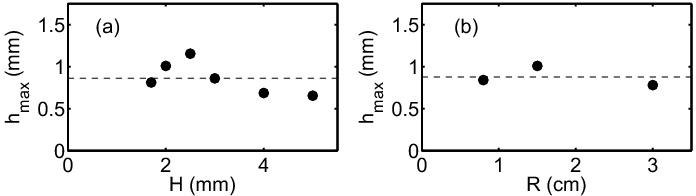
Figure 13: Dependence of distension size $h_{\mathrm{max}}$ on geometric parameters. LP experiments with a bulk concentration of PDMS. ($a$) For fixed $R=1.5$ cm and varying $H$ (second row of Table 2), with $\langle h_{\mathrm{max}}\rangle=0.86$ mm (dashed line). ($b$) For fixed $H=2$ mm and varying $R$ (third row of Table 2), with $\langle h_{\mathrm{max}}\rangle=0.88$ mm (dashed line).

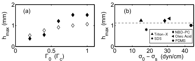
Figure 14: Dependence of distension size $h_{\mathrm{max}}$ on material parameters. Simulations (open symbols) and both FI/LP and LP experiments (closed symbols). ($a$) Experiments and redimensionalized simulations with a variety of initial concentrations of NBD-PC and fixed $H=0.7$ mm and $R=3.0$ cm (first row of Table 2). ($b$) Experiments on five surfactant types, with fixed $R=1.5$ cm, $H=2.0$ mm, and $V=540\,\mu$L (fourth row of Table 2). $\sigma_{0}-\sigma_{S}$ quantifies the surface tension contrast for each surfactant. Dashed line is $\langle h_{\mathrm{max}}\rangle=1.12$ mm.

First, we perform experiments using a bulk quantity of PDMS as the surfactant, and probe the geometric effects using LP. We either vary the initial underlying glycerin thickness $H$ or the retaining ring radius $R$ while leaving all other variables constant. As shown in Fig. 13, we observe a millimetric distension height in all cases with no systematic dependence on either $H$ or $R$.

Second, we perform experiments and simulations examining the effects of different surfactant materials and concentrations, using a combination of LP and FI/LP experiments. As shown in Fig. 14$a$, we vary the concentration of NBD-PC while leaving $R$ and $H$ constant. We observe semi-quantitative agreement between the predicted and observed values of $h_{\mathrm{max}}$ which increase as we increase $\Gamma_{0}$. In Fig. 14$b$, we examine the full collection of bulk surfactants, which includes soluble (Triton X-305, SDS), insoluble (PDMS, oleic acid, NBD-PC), non-ionic (Triton X-305, PDMS), anionic (SDS, oleic acid), and zwitterionic (NBD-PC) surfactants, using a fixed volume of surfactant in a fixed geometry. In spite of this large parameter space, we find little dependence of $h_{\mathrm{max}}$ on the surface tension difference. This may be due to the existence of a large reservoir of bulk surfactant which is not present in the monolayer experiments.

IV Discussion and Conclusions

In the axisymmetric self-healing of a surfactant layer on a thin fluid film, gradients in the surfactant distribution generate Marangoni forces which drive the fluid towards the center of the surfactant-free region. The surface motion of the fluid advects the surfactant, while the bulk motion of the incompressible fluid pushes up an annular Marangoni ridge which coalesces into a central distension. This distension reaches a maximum height, after which it decays.

We approach this self-healing system in two ways. First, we use a combination of fluorescence imaging and laser profilometry to simultaneously probe the dynamics of both the fluid height and surfactant concentration profiles. We find that while the commonly-used model by Gaver and Grotberg (1990), together with the equation of state by Borgas and Grotberg (2006), predicts reasonable fluid height profile shapes, it does not accurately predict the spatial distribution of surfactant. The agreement in the fluid height profile suggests the validity of the lubrication approximation for this system. In addition, the model correctly predicts the approximate shape of both $r_{M}(t)$ and $r_{S}(t)$. Further, our measurements of $r_{S}$ give validity to Jensen’s prediction Jensen (1994) of $r_{S}\propto(t_{c}-t)^{0.81}$. At present, it remains unclear to what extent the deviations in the surfactant concentration profile, the presence of a meniscus, and the uncertainty in the glycerin viscosity each contribute to the disagreement in the timescale. Second, we probe the generality of the effect, beyond the model’s assumptions. Using laser profilometry, we probe dependence of the distension height on the initial fluid thickness, initial hole size, type of surfactant, and surfactant concentration. In all cases, the distension was millimetric in size, and only changes in the concentration of surfactant were able to produce different $h_{\mathrm{max}}$.

In both these results and the droplet-spreading results of Swanson et al. (2013), the experiments exhibited different behaviors at low surfactant concentrations: the Marangoni ridge was suppressed, and the surfactant spreading drastically slowed. In addition, simulations are not able to capture the sharp leading edge of our inward-spreading front. These findings suggest that the commonly-used linear or multilayer equations of state are insufficient to capture low-$\Gamma$ dynamics (Peterson, 2010). A promising future direction would be to incorporate an empirically-determined equation of state. Another interesting direction of investigation would be to probe the effect of the fluid meniscus created as the ring lifts. The observations presented in Fig. 7 indicate that surfactant molecules coalesce at the meniscus as the ring is slowly lifted, and leave behind an excess of surfactant that persists after pinch-off and propagates inward. For a linear equation of state, the incorporation of a meniscus and a small surfactant excess near the ring does not have a significant effect on the profiles or dynamics in numerical simulations (Swanson et al., 2013). Again, an emperically-determined equation of state might provide additional insight into the real effects of the meniscus.

Based upon the lack of self-healing for dilute initial conditions (0.2 $\Gamma_{c}$), we conclude that there is either no Marangoni force present, or that there are additional counterbalancing forces not accounted in the model. For example, an equation of state with a vanishing derivative below a threshold value of $\Gamma$ would produce no Marangoni force. For NBD-PC, our experiments suggest that this threshold would be between $0.2$ and $0.4\,\Gamma_{c}$. Such an equation of state would additionally explain the sharpness of the surfactant leading edge for both droplet spreading (Swanson et al., 2013) and self-healing. In both cases, when the concentration at the leading edge falls below this threshold, then the Marangoni force at the leading edge vanishes and can no longer act to broaden it. However, an equation of state with a vanishing derivative is likely not the complete story. As discussed by Kaganer et al. (1999) for quasi-static systems, surfactant in sparse concentrations undergoes a liquid-gas phase transition. The sparse gas phase is characterized by a two dimensional ideal gas law which stipulates that $\sigma(\Gamma)$ should be linear. This provides a non-vanishing derivative for the equation of state. It may therefore be necessary to also consider restoring forces such as surface elasticity which are not present in the Gaver and Grotberg (1990) model.

The novel surfactant fluorescence visualization techniques developed in (Swanson et al., 2013) and used in this work have finally allowed us to make quantitative comparisons to the well-accepted Gaver and Grotberg (1990) model . We see clearly the success of this model in implementing the lubrication approximation, and we have explained how this well-accepted model would benefit from incorporating a more physically-motivated model of the surfactant monolayer.

V Acknowledgments

This work was funded by the NSF grant DMS-FRG #0968154 and the Research Corporation Cottrell Scholar Award #19788. We thank Kali Allison for conducting the initial experiments on this system, Jonathan Claridge and Jeffrey Wong for collaboration on the code, and Michael Shearer and Ellen Swanson for insightful conversations.

References

- Franklin et al. [1774] B. Franklin, W. Brownrigg, and Farish. Of the stilling of waves by means of oil. Philos. Trans. R. Soc. Lond., 64:445, 1774.
- Rayleigh and Pockels [1891] Lord Rayleigh and A. Pockels. Surface tension. Nature, 43(1115):437, 1891.
- Kaganer et al. [1999] V. Kaganer, H. Möhwald, and P. Dutta. Structure and phase transitions in Langmuir monolayers. Rev. Mod. Phys., 71(3):779, 1999.
- Hoult [1972] D. P. Hoult. Oil spreading on the sea. Annu. Rev. Fluid Mech., 4(1):341, 1972.
- Gaver and Grotberg [1990] D. P. Gaver and J. B. Grotberg. The dynamics of a localized surfactant on a thin film. J. Fluid Mech., 213:127, 1990.
- Gaver and Grotberg [1992] D. P. Gaver and J. B. Grotberg. Droplet spreading on a thin viscous film. J. Fluid Mech., 235:399, 1992.
- Braun [2012] R. J. Braun. Dynamics of the tear film. Annu. Rev. Fluid Mech., 44:267, 2012.
- Maki et al. [2010] K. L. Maki, R. J. Braun, P. Ucciferro, W. D. Henshaw, and P. E. King-Smith. Tear film dynamics on an eye-shaped domain. part 2. flux boundary conditions. J. Fluid Mech., 647:361, 2010.
- Jensen et al. [1994] O. E. Jensen, D. Halpern, and J. B. Grotberg. Transport of a passive solute by surfactant-driven flows. Chem. Eng. Sci., 49(8):1107, 1994.
- Evans et al. [2000] P. L. Evans, L. W. Schwartz, and R. V. Roy. A mathematical model for crater defect formation in a drying paint layer. J. Colloid Interf. Sci., 227(1):191, 2000.
- Gundabala et al. [2008] V. R. Gundabala, C. Lei, K. Ouzineb, O. Dupont, J. L. Keddie, and A. F. Routh. Lateral surface nonuniformities in drying latex films. AICHE J., 54(12):3092, 2008.
- Gundabala and Routh [2006] V. R. Gundabala and A. F. Routh. Thinning of drying latex films due to surfactant. J. Colloid Interf. Sci., 303(1):306, 2006.
- Hanyak et al. [2011] M. Hanyak, A. A. Darhuber, and M. Ren. Surfactant-induced delay of leveling of inkjet-printed patterns. J. Appl. Phys., 109(7):074905, 2011.
- Hanyak et al. [2012] M. Hanyak, D. K. N. Sinz, and A. A. Darhuber. Soluble surfactant spreading on spatially confined thin liquid films. Soft Matter, 8(29):7660, 2012.
- Sinz et al. [2011] D. K. N. Sinz, M. Hanyak, J. C. H. Zeegers, and A. A. Darhuber. Insoluble surfactant spreading along thin liquid films confined by chemical surface patterns. Phys. Chem. Chem. Phys., 13(20):9768, 2011.
- Craster and Matar [2007] R. V. Craster and O. K. Matar. On autophobing in surfactant-driven thin films. Langmuir, 23(5):2588, 2007.
- Jensen and Grotberg [1992] O. E. Jensen and J. B. Grotberg. Insoluble surfactant spreading on a thin viscous film: shock evolution and film rupture. J. Fluid Mech., 240:259, 1992.
- Espinosa et al. [1993] F. F. Espinosa, A. H. Shapiro, J. J. Fredberg, and R. D. Kamm. Spreading of exogenous surfactant in an airway. J. Appl. Physiol., 75(5):2028, 1993.
- Levy and Shearer [2006] R. Levy and M. Shearer. The motion of a thin liquid film driven by surfactant and gravity. Siam J. Appl. Math, 66(5):1588, 2006.
- Dussaud and Troian [1998] A. D. Dussaud and S. M. Troian. Dynamics of spontaneous spreading with evaporation on a deep fluid layer. Phys. Fluids, 10(1):23, 1998.
- Dussaud et al. [2005] A. D. Dussaud, O. K. Matar, and S. M. Troian. Spreading characteristics of an insoluble surfactant film on a thin liquid layer: comparison between theory and experiment. J. Fluid Mech., 544:23, 2005.
- Fallest et al. [2010] D. W. Fallest, A. M. Lichtenberger, C. J. Fox, and K. E. Daniels. Fluorescent visualization of a spreading surfactant. New J. Phys., 12:073029, 2010.
- Bull et al. [1999] J. L. Bull, L. K. Nelson, J. T. Walsh, M. R. Glucksberg, S. Schürch, and J. B. Grotberg. Surfactant-spreading and surface-compression disturbance on a thin viscous film. J. Biomech. Eng-T ASME, 121(1):89, 1999.
- Swanson et al. [2013] E. R. Swanson, S. L. Strickland, M. Shearer, and K. E. Daniels. Surfactant spreading on a thin liquid film: reconciling models and experiments. Preprint arXiv:1306.4881, 2013.
- Troian et al. [1989] S. M. Troian, X. L. Wu, and S. A. Safran. Fingering instability in thin wetting films. Phys. Rev. Lett., 62(13):1496, 1989.
- Hamraoui et al. [2004] A. Hamraoui, M. Cachile, C. Poulard, and A. M. Cazabat. Fingering phenomena during spreading of surfactant solutions. Colloid Surface A, 250(1-3):215, 2004.
- Jensen [1994] O. E. Jensen. Self-similar, surfactant-driven flows. Phys. Fluids, 6(3):1084, 1994.
- Segur and Oberstar [1951] J. B. Segur and H. E. Oberstar. Viscosity of glycerol and its aqueous solutions. Ind. Eng. Chem., 43(9):2117, 1951.
- Bosart and Snoddy [1928] L. W. Bosart and A. O. Snoddy. Specific gravity of glycerol. Ind. Eng. Chem., 20(12):1377, 1928.
- Gallant [1967] R. W. Gallant. Physical properties of hydrocarbons. Hydrocarb. Process., 46(5):201, 1967.
- Mysels [1986] K. J. Mysels. Surface tension of solutions of pure sodium dodecyl sulfate. Langmuir, 2(4):423, 1986.
- Agrawal and Neuman [1988] M. L. Agrawal and R. D. Neuman. Surface diffusion in monomolecular films: Ii. experiment and theory. J. Colloid Interf. Sci., 121(2):366, 1988.
- Sakata and Berg [1969] E. K. Sakata and J. C. Berg. Surface diffusion in monolayers. Ind. Eng. Chem. Fund., 8(3):570, 1969.
- Shrive et al. [1995] J. D. A. Shrive, J. D. Brennan, R. S. Brown, and U. J. Krull. Optimization of the self-quenching response of nitrobenzoxadiazole dipalmitoylphosphatidylethanolamine in phospholipid membranes for biosensor development. Appl. Spectrosc., 49(3):304, 1995.
- Peterson [2010] Ellen R Peterson. Flow of Thin Liquid Flims with Surfactant: Analysis, Numerics, and Experiment. PhD thesis, North Carolina State University, 2010.
- Borgas and Grotberg [2006] M. S. Borgas and J. B. Grotberg. Monolayer flow on a thin film. J. Fluid Mech., 193:151, 2006.
- Claridge et al. [2013] J. Claridge, R. Levy, and J. Wong. Solving nonlinear high-order pde systems: Methodology and a clawpack library. Preprint, 2013.
- Kronmiller et al. [2013] G Kronmiller, E. Autry, and C. Conti. The effects of spatial and temporal grids on simulations of thin films with surfactant. SIURO, 6:81, 2013.