Optimal continuous variable quantum teleportation protocol for realistic settings

Abstract

We show the optimal setup that allows Alice to teleport coherent states $|\alpha\rangle$ to Bob giving the greatest fidelity (efficiency) when one takes into account two realistic assumptions. The first one is the fact that in any actual implementation of the continuous variable teleportation protocol (CVTP) Alice and Bob necessarily share non-maximally entangled states (two-mode finitely squeezed states). The second one assumes that Alice’s pool of possible coherent states to be teleported to Bob does not cover the whole complex plane ($|\alpha|<\infty$). The optimal strategy is achieved by tuning three parameters in the original CVTP, namely, Alice’s beam splitter transmittance and Bob’s displacements in position and momentum implemented on the teleported state. These slight changes in the protocol are currently easy to be implemented and, as we show, give considerable gain in performance for a variety of possible pool of input states with Alice.

1 Introduction

The extension of the quantum teleportation protocol from discrete (finite dimensional Hilbert spaces) [1] to continuous variable (CV) (infinite dimension) systems was a landmark to CV quantum communication [2, 3, 4]. The main goal of teleportation is to make sure that at the end of the whole protocol a quantum state originally describing Alice’s system turns out to describe a quantum system with Bob at a different location. Moreover, no direct transmission of the system from Alice to Bob is done and the knowledge of Alice’s system is not needed at all to accomplish such a task. These two properties clearly illustrate why teleportation is so powerful a tool. Indeed, for quantum teleportation take place Alice and Bob only need to be able to act locally on their systems, communicate classically and share a quantum channel (entangled state). At the end of the process Alice’s system is no longer described by its original state that now describes Bob’s system.

In principle, a perfect teleportation only occurs when Alice and Bob share a maximally entangled state. By perfect teleportation we mean that at the end of the protocol and with probability one Bob’s system will be exactly described by the state that originally described Alice’s system. For discrete systems, and in particular for qubits, such maximally entangled states (Bell states) that Alice and Bob must share can be experimentally generated in the laboratory [5, 6]. For CV-systems, however, the perfect implementation of the teleportation protocol [3] requires a maximally entangled state (the Einstein-Podolsky-Rosen (EPR) state) that cannot be generated in the laboratory [7, 8, 9]. In modern quantum optics terminology, one needs an entangled two-mode squeezed state with infinite squeezing ($r\rightarrow\infty$). For finite squeezing ($r<\infty$), the teleported quantum state at Bob’s is never identical to the original one at Alice’s.

Another assumption in the usual teleportation protocols is related to the pool of input states available to Alice, i.e., the states that Alice might choose to teleport to Bob. For example, consider the simplest discrete system, a qubit. In this case it is assumed that Alice’s input is given by $|\varphi\rangle=a|0\rangle+b|1\rangle$, with $a$ and $b$ random complex numbers satisfying the normalization condition $|a|^{2}+|b|^{2}=1$. For CV systems, and in particular for coherent states $|\alpha\rangle$, with $\alpha$ complex, it is often assumed that Alice’s pool of states cover the entire complex plane [3, 10, 11]. From a theoretical point of view, either for a qubit or a coherent state, these assumptions are the proper ones in order to determine the strictest conditions guaranteeing a “truly” quantum teleportation, i.e., the conditions where no purely classical protocol can achieve the same efficiency as those predicted by the quantum ones [11, 12]. From a practical point of view, however, these assumptions are only valid for qubits, being unrealistic for CV systems. Indeed, the energy of a coherent state is proportional to $|\alpha|^{2}$ and in order to cover the entire complex plane we would need states with infinite energy. Also, the greater $|\alpha|$ the less quantum a coherent state becomes [13] and other techniques than quantum teleportation such as a direct transmission of the state may be better suited in this case.

With these two realistic assumptions in mind, a natural question then arises. Is it possible to further improve the efficiency of the standard CV teleportation protocol (CVTP) by taking into account in any modification of the original setup [3] these two facts?

For a pool of input coherent states with Alice described by a Gaussian distribution centered at the vacuum state [14] and when Alice is always teleporting a fixed single state [15, 16, 17], the answer to the previous question is affirmative. In standard modifications of the CVTP [14, 15], only a single parameter is freely adjusted in order to improve the quality of the teleported state: Bob is free to choose the gain $g$ that he might apply equally to the quadratures of his mode at the end of the protocol (see figure 1). In the original setup $g=1$, while in the modified versions it was tuned as a function of the input states and of the squeezing of the channel in order to increase the efficiency of CVTP. An identical strategy was employed to improve the efficiency of CV entanglement swapping [18, 19], where the optimal $g$ was tuned for a specific input state.

What would happen if we go beyond a Gaussian probability distribution centered at the vacuum and use instead uniform distributions or distributions centered in the coherent state $|\beta\rangle$, $\beta\neq 0$? More important, what are the optimal conditions if we introduce more than one free parameter in the modified version of CVTP [16], where either Alice or Bob can change the protocol? Our goal here is to investigate these two questions in detail and without assuming we know the state to be teleported [16, 17]. The only knowledge we have is the probability of Alice picking a particular coherent state $|\alpha\rangle$ according to a predefined probability distribution. In other words, Alice and Bob know a priori the probability distribution describing the possible set of states to be teleported, but not the actual state at a given execution of the protocol.

In what follows we show that it is possible to achieve further significant increase in performance with extra free parameters that introduce, however, minimal changes to the original scheme, modifications of which can already be implemented in the laboratory. Also, some of the optimal settings are counterintuitive and not found in standard modifications of CVTP. For instance, sometimes it is better to use an unbalanced beam splitter (BS) instead of a balanced one when Alice combines her share of the entangled channel with the state to be teleported.

We also investigate several probability distributions describing the input states and we show the optimal modifications to each one of them. Moreover, the optimal parameters change appreciably if we work with either uniform or Gaussian distribution or if those distributions are centered or not on the vacuum state. And as expected, the changes in the original CVTP not only depend on the specific probability distribution associated to Alice’s input states but also on the entanglement of the channel.

2 Formalism

2.1 Qualitative analysis

Before diving into the mathematical details of our calculations, it is worth presenting the bigger picture, i.e., the choices we made from the start in order to modify the original setup and the strategy employed to determine the optimal teleportation protocol.

In the original proposal (see figure 1), a two-mode squeezed state with squeezing $r$, our entanglement resource, is shared between Alice and Bob. Mode $2$ goes to Alice and mode $3$ to Bob. The state with Alice to be teleported is represented by mode $1$, which can be any coherent state $|\alpha\rangle$. To proceed with the teleportation, Alice combines modes $1$ and $2$ in a $50\!\!:\!\!50$ BS and afterwards measures the position and momentum (quadratures of the electromagnetic field) of modes $u$ and $v$, respectively, whose results $\tilde{x}_{u}$ and $\tilde{p}_{v}$ are then classically communicated to Bob. With this information he displaces in position ($x_{3}\rightarrow x_{3}+g\sqrt{2}\tilde{x}_{u}$) and momentum ($p_{3}\rightarrow p_{3}+g\sqrt{2}\tilde{p}_{v}$) his mode to get the right teleported state. The displacements and gain $(g=1)$ are chosen and fixed as the ones yielding perfect teleportation when $r\rightarrow\infty$ (maximal entanglement).

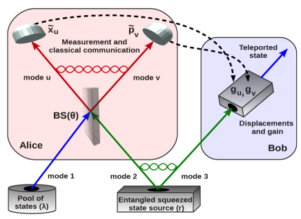
Figure 1: In the original proposal [3] we have $\theta=\pi/4$ ($50:50$ BS), $g_{u}=g_{v}=g\sqrt{2}$, with $g=1$, and position and momentum displacements given by $x_{3}\rightarrow x_{3}+g_{u}\tilde{x}_{u}$ and $p_{3}\rightarrow p_{3}+g_{v}\tilde{p}_{v}$. These choices yield an average fidelity $F_{av}$ independent of whatever pool of states (labeled by $\lambda$) is available to Alice. Here, for fixed $\lambda$ and squeezing $r$, the optimization to get the optimal $F_{av}$ is implemented over three free parameters, $\theta,g_{v}$, and $g_{u}$, leading to $F_{av}$ that depends both on $r$ and $\lambda$. See text for details.

A priory there is no guarantee that the previous choices for the BS transmittance ($\cos^{2}\theta=1/2$), displacements and gain are the optimal ones for all combinations of finite squeezing $r$ and probability distribution for the pool of states available to Alice. Therefore, in order to search for the optimal protocol for a given squeezing $r$ and probability distribution we allow the BS to have an arbitrary transmittance ($BS(\theta)$), with $0<\theta<\pi/2$ (see figure 1). Furthermore, the quadratures’ displacements and gain $g$ that Bob must implement after Alice informs him of her measurement results ($\tilde{x}_{u}$ and $\tilde{p}_{v}$) [3, 10] are also independently chosen in order to optimize the protocol. Formally, Bob’s displacements are given by $x_{3}\rightarrow x_{3}+g_{u}\tilde{x}_{u}$ and $p_{3}\rightarrow p_{3}+g_{v}\tilde{p}_{v}$, with $g_{u}$ and $g_{v}$ chosen in order to optimize the efficiency of CVTP.

2.2 Quantitative analysis

2.2.1 The protocol.

In what follows we present the details of the mathematical analysis of the modified CVTP, where the three parameters described above are incorporated into the protocol. We use interchangeably the words kets, states, and modes to refer to the same object, namely, the quantized electromagnetic modes [10]. Also, when we refer to position $\hat{x}_{k}=(\hat{a}_{k}+\hat{a}_{k}^{\dagger})/2$ and momentum $\hat{p}_{k}=(\hat{a}_{k}-\hat{a}_{k}^{\dagger})/2i$, with $\hat{a}_{k}$ and $\hat{a}_{k}^{\dagger}$ annihilation and creation operators, we mean the quadratures of mode $k$, with commutation relation $[\hat{x}_{k},\hat{p}_{k}]=i/2$.

An arbitrary input state with Alice can be written in the position basis as

$$|\varphi\rangle=\int dx_{1}\varphi(x_{1})|x_{1}\rangle,$$ (1)

where $\varphi(x_{1})=\langle x_{1}|\varphi\rangle$ and the integration runs over the entire real line. The entangled state shared between Alice and Bob can also be written in the position basis as

$$|\Phi\rangle=\int dx_{2}dx_{3}\Phi(x_{2},x_{3})|x_{2},x_{3}\rangle,$$ (2)

with $\Phi(x_{2},x_{3})=\langle x_{2},x_{3}|\Phi\rangle$ and $|x_{2},x_{3}\rangle=|x_{2}\rangle\otimes|x_{3}\rangle$. Unless stated otherwise, we keep the ordering of the kets fixed, i.e, the notation $|x_{1},x_{2},x_{3}\rangle$ means that the first two modes/kets are with Alice and the third one with Bob. Using equations (1) and (2) we can write the initial state describing all modes before the beginning of the teleportation protocol as $|\Psi\rangle=|\varphi\rangle\otimes|\Phi\rangle$, or more explicitly,

$$|\Psi\rangle=\int dx_{1}dx_{2}dx_{3}\varphi(x_{1})\Phi(x_{2},x_{3})|x_{1},x_{2},x_{3}\rangle.$$ (3)

The first step in the protocol consists in sending mode 1 (input state) and mode 2 (Alice’s share of the two-mode squeezed state) to a BS with transmittance $\cos^{2}\theta$ (see figure 1). Calling $\hat{B}_{12}(\theta)$ the operator representing the action of the BS we have in the position basis [10]

$$\hat{B}_{12}(\theta)|x_{1},x_{2}\rangle=|x_{1}\sin\theta+x_{2}\cos\theta,x_{1}\cos\theta-x_{2}\sin\theta\rangle.$$ (4)

Inserting equation (4) into (3) and making the following variable changes, $x_{v}=x_{1}\sin\theta+x_{2}\cos\theta$ and $x_{u}=x_{1}\cos\theta-x_{2}\sin\theta$, we have

$$|\Psi^{\prime}\rangle = \int dx_{v}dx_{u}dx_{3}\varphi(x_{v}\sin\theta+x_{u}\cos\theta)\Phi(x_{v}\cos\theta-x_{u}\sin\theta,x_{3})|x_{v},x_{u},x_{3}\rangle$$ (5)

for the total state after modes $1$ and $2$ go through $BS(\theta)$.

The next step of the protocol consists in measuring the momentum and position of modes $v$ and $u$, respectively. For the quantized electromagnetic mode, this is achieved by homodyne detectors yielding classical photocurrents that assign real numbers for the quadratures $\hat{p}_{v}$ and $\hat{x}_{u}$ [10].

Since Alice will project mode $v$ onto the momentum basis, it is convenient to rewrite equation (5) using the Fourier transformation relating the position and momentum eigenstates,

$$|x_{v}\rangle=\frac{1}{\sqrt{\pi}}\int dp_{v}e^{-2ix_{v}p_{v}}|p_{v}\rangle.$$ (6)

Thus, inserting equation (6) into (5) we have

$$|\Psi^{\prime}\rangle = \frac{1}{\sqrt{\pi}}\int dp_{v}dx_{v}dx_{u}dx_{3}\varphi(x_{v}\sin\theta+x_{u}\cos\theta)\Phi(x_{v}\cos\theta-x_{u}\sin\theta,x_{3})e^{-2ix_{v}p_{v}}|p_{v},x_{u},x_{3}\rangle.$$

(7)

In the second step of the protocol, Alice measures the momentum of mode $v$ and the position of mode $u$ (see figure 1). Assuming her measurement results are $\tilde{p}_{v}$ and $\tilde{x}_{u}$, the total state at the end of the measurement is simply obtained applying the measurement postulate of quantum mechanics,

$$|\Psi^{\prime\prime}\rangle=\hat{P}_{\tilde{p}_{v},\tilde{x}_{u}}|\Psi^{\prime}\rangle/\sqrt{\mathbb{p}(\tilde{p}_{v},\tilde{x}_{u})},$$

where $\hat{P}_{\tilde{p}_{v},\tilde{x}_{u}}=|\tilde{p}_{v},\tilde{x}_{u}\rangle\langle\tilde{p}_{v},\tilde{x}_{u}|\otimes\mathbb{1}_{3}$ is the projector describing the measurements and $\mathbb{1}_{3}$ is the identity operator acting on mode $3$. Also,

$$\mathbb{p}(\tilde{p}_{v},\tilde{x}_{u})={\rm tr}\;(|\Psi^{\prime}\rangle\langle\Psi^{\prime}|\hat{P}_{\tilde{p}_{v},\tilde{x}_{u}})$$

is the probability of measuring momentum $\tilde{p}_{v}$ and position $\tilde{x}_{u}$, with ${\rm tr}\;$ denoting the total trace. Specifying to the position basis and noting that $\langle p_{v}|\tilde{p}_{v}\rangle=\delta(p_{v}-\tilde{p}_{v})$ and $\langle x_{u}|\tilde{x}_{u}\rangle=\delta(x_{u}-\tilde{x}_{u})$ we have

$$|\Psi^{\prime\prime}\rangle=|\tilde{p}_{v},\tilde{x}_{u}\rangle\otimes|\chi^{\prime}\rangle,$$ (8)

where Bob’s state is

$$|\chi^{\prime}\rangle = \frac{1}{\sqrt{\pi\mathbb{p}(\tilde{p}_{v},\tilde{x}_{u})}}\int dx_{v}dx_{3}\varphi(x_{v}\sin\theta+\tilde{x}_{u}\cos\theta)\Phi(x_{v}\cos\theta-\tilde{x}_{u}\sin\theta,x_{3})e^{-2ix_{v}\tilde{p}_{v}}|x_{3}\rangle.$$ (9)

Here

$$\mathbb{p}(\tilde{p}_{v},\tilde{x}_{u})=\int dx_{3}|\Psi^{\prime}(\tilde{p}_{v},\tilde{x}_{u},x_{3})|^{2}$$ (10)

and

$$\Psi^{\prime}(\tilde{p}_{v},\tilde{x}_{u},x_{3})=\langle\tilde{p}_{v},\tilde{x}_{u},x_{3}|\Psi^{\prime}\rangle=\frac{1}{\sqrt{\pi}}\int dx_{v}\varphi(x_{v}\sin\theta+\tilde{x}_{u}\cos\theta)\Phi(x_{v}\cos\theta-\tilde{x}_{u}\sin\theta,x_{3})e^{-2ix_{v}\tilde{p}_{v}},$$ (11)

where equation (11) was obtained using (7).

The third step of the protocol consists in Alice sending to Bob via a classical channel (photocurrents) her measurement results. With this information Bob is able to implement the fourth and last step of the protocol, namely, he displaces his mode quadratures according to the following rule, $x_{3}\rightarrow x_{3}+g_{u}\tilde{x}_{u}$ and $p_{3}\rightarrow p_{3}+g_{v}\tilde{p}_{v}$. Mathematically, this corresponds to the application of the displacement operator $\hat{D}(\alpha)=e^{\alpha\hat{a}^{\dagger}-\alpha^{*}\hat{a}}=e^{-2iRe[\alpha]\hat{p}+2iIm[\alpha]\hat{x}}$, with $\alpha=g_{u}\tilde{x}_{u}+ig_{v}\tilde{p}_{v}$. Since $\hat{x}$ and $\hat{p}$ commute with their commutator we can apply Glauber’s formula to obtain $\hat{D}(\alpha)=e^{iRe[\alpha]Im[\alpha]}e^{-2iRe[\alpha]\hat{p}}e^{2iIm[\alpha]\hat{x}}$. This leads to

$$\hat{D}(g_{u}\tilde{x}_{u}+ig_{v}\tilde{p}_{v})|x_{3}\rangle=e^{ig_{u}g_{v}\tilde{x}_{u}\tilde{p}_{v}}e^{2ig_{v}\tilde{p}_{v}x_{3}}|x_{3}+g_{u}\tilde{x}_{u}\rangle.$$ (12)

The final state with Bob, $|\chi\rangle=\hat{D}(g_{u}\tilde{x}_{u}+ig_{v}\tilde{p}_{v})|\chi^{\prime}\rangle$, can be put as follows if we use equation (12) and make the variable change $x_{3}\rightarrow x_{3}-g_{u}\tilde{x}_{u}$,

$$|\chi\rangle = \frac{e^{-ig_{u}g_{v}\tilde{x}_{u}\tilde{p}_{v}}}{\sqrt{\pi\mathbb{p}(\tilde{p}_{v},\tilde{x}_{u})}}\int dx_{v}dx_{3}\varphi(x_{v}\sin\theta+\tilde{x}_{u}\cos\theta)$$ (13)

$$\times\Phi(x_{v}\cos\theta-\tilde{x}_{u}\sin\theta,x_{3}-g_{u}\tilde{x}_{u})e^{-2i(x_{v}-g_{v}x_{3})\tilde{p}_{v}}|x_{3}\rangle$$

$$= \int dx_{3}\left(\frac{e^{-ig_{u}g_{v}\tilde{x}_{u}\tilde{p}_{v}}}{\sqrt{\pi\mathbb{p}(\tilde{p}_{v},\tilde{x}_{u})}}\int dx_{v}\varphi(x_{v}\sin\theta+\tilde{x}_{u}\cos\theta)\right.$$

$$\left.\times\Phi(x_{v}\cos\theta-\tilde{x}_{u}\sin\theta,x_{3}-g_{u}\tilde{x}_{u})e^{-2i(x_{v}-g_{v}x_{3})\tilde{p}_{v}}\right)|x_{3}\rangle$$

$$= \int dx_{3}\chi(x_{3})|x_{3}\rangle.$$

Note that $e^{-ig_{u}g_{v}\tilde{x}_{u}\tilde{p}_{v}}$ in Bob’s final state is an irrelevant global phase and could be suppressed.

It is worth mentioning at this point that equation (13), together with equations (10) and (11), are quite general. They allow us to get the teleported state with Bob for any input state and any entangled state (channel) shared between Alice and Bob. For instance, if we use a maximally entangled state (EPR state) we have [10] $\Phi(x_{2},x_{3})\propto\delta(x_{2}-x_{3})$ in equation (2). Using this channel in equation (13) leads to $\chi(x_{3})=\varphi(x_{3})$ if we set $g_{u}=g_{v}=\sqrt{2}$ and $\theta=\pi/4$, i.e, we have a perfect teleportation.

2.2.2 Fidelity.

As a figure of merit to decide the optimality of the protocol we employ the average fidelity $F_{av}$ [11], whose computation requires the specification of the presumed probability of available states with Alice, assumed fixed throughout the many runs of the protocol. The fidelity measures how close the output state with Bob at the end of the protocol is to the input state employed by Alice. Here the average is taken over the fidelities of each input state and its respective output, with the weight of each state given by its probability to be picked out of the states available to Alice. Our strategy consists, therefore, in choosing $\theta,g_{v}$, and $g_{u}$ in order to maximize $F_{av}$.

Mathematically, if the density matrix describing the output state with Bob after one single run of the protocol is $\hat{\rho}_{B}=|\chi\rangle\langle\chi|$, the fidelity is defined as

$$F(|\varphi\rangle,\tilde{p}_{v},\tilde{x}_{u})=\langle\varphi|\hat{\rho}_{B}|\varphi\rangle,$$ (14)

where we highlight that the fidelity depends on the input state $|\varphi\rangle$ and on the measurement outcomes obtained by Alice. For the moment we leave implicit the dependence on the other parameters, i.e, what channel/entanglement we have and $\theta$, $g_{v}$, and $g_{u}$. Note that $F$ achieves its maximal value (one) only if we have a flawless teleportation ($\hat{\rho}_{B}=\hat{\rho}_{input}$) and its minimal one (zero) if the output is orthogonal to the input.

At each run of the protocol, Alice will measure $\tilde{p}_{v}$ and $\tilde{x}_{u}$ with probability $\mathbb{p}(\tilde{p}_{v},\tilde{x}_{u})$. Hence, Bob’s final ensemble of states, averaged over all possible measurement results for a fixed input state $|\varphi\rangle$, is

$$F(|\varphi\rangle)=\int d\tilde{p}_{v}d\tilde{x}_{u}\mathbb{p}(\tilde{p}_{v},\tilde{x}_{u})F(|\varphi\rangle,\tilde{p}_{v},\tilde{x}_{u}).$$ (15)

Furthermore, to properly search the optimal configuration for a probability distribution of input states $P(|\varphi\rangle)$ with Alice, another averaging is needed, this time over the pool of states available to her [11],

$$F_{av}(\theta,g_{v},g_{u})=\int d|\varphi\rangle P(|\varphi\rangle)F(|\varphi\rangle).$$ (16)

The strategy to optimize the teleportation protocol, once we know $P(|\varphi\rangle)$, is the search for the triple of points $(\theta,g_{v},g_{u})$ maximizing $F_{av}(\theta,g_{v},g_{u})$. Therefore, for fixed entanglement, we either solve analytically (if possible) or numerically the following three equations for $\theta,g_{v},$ and $g_{u}$,

$$\frac{\partial F_{av}}{\partial\theta}=0,\hskip 8.5359pt\frac{\partial F_{av}}{\partial g_{v}}=0,\hskip 8.5359pt\frac{\partial F_{av}}{\partial g_{u}}=0.$$ (17)

The obtained solutions are then inserted into (16) and slightly varied about their actual values in order to be sure we have a global maximum, ruling out possible local maximums, minimums, and saddle points.

3 Results

In the rest of this paper we particularize to input states at Alice’s given by coherent states,

$$|\varphi\rangle=|\alpha\rangle,$$

with $\alpha$ complex, and to the entanglement shared between Alice and Bob given by two-mode squeezed vacuum states,

$$|\Phi\rangle=|\psi_{r}\rangle=\sqrt{1-\tanh^{2}r}\sum_{n=0}^{\infty}\tanh^{n}r|n\rangle_{A}\otimes|n\rangle_{B},$$

where $|n\rangle_{A(B)}$ are Fock number states at Alice’s (Bob’s). Also, $r$ is the squeezing parameter and for $r=0$ we have $|00\rangle$, the vacuum state, and for $r\rightarrow\infty$ the unphysical maximally entangled EPR state. Both coherent and two-mode squeezed states of the quantized electromagnetic field are easily generated in the laboratory today and they were the ingredients employed in the experimental implementation of the original CVTP [7].

These two states are represented in the position basis as [10]

$$\phi(x_{1})=\langle x_{1}|\alpha\rangle=\left(\frac{2}{\pi}\right)^{1/4}e^{-x_{1}^{2}+2\alpha x_{1}-|\alpha|^{2}/2-\alpha^{2}/2}$$ (18)

and

$$\Phi(x_{2},x_{3}) = \langle x_{2},x_{3}|\psi_{r}\rangle=\sqrt{\frac{2}{\pi}}\exp\left[-e^{-2r}(x_{2}+x_{3})^{2}/2-e^{2r}(x_{2}-x_{3})^{2}/2\right].$$ (19)

Equations (18) and (19) allow us to explicitly compute equation (15),

$$F(|\alpha\rangle)=f_{2}(\theta,g_{v})^{-\frac{1}{2}}\exp\left[-\frac{f_{1}(\theta,g_{v})}{f_{2}(\theta,g_{v})}Im[\alpha]^{2}\right]f_{2}\left(\theta-\frac{\pi}{2},g_{u}\right)^{-\frac{1}{2}}\exp\left[-\frac{f_{1}(\theta+\frac{\pi}{2},g_{u})}{f_{2}(\theta-\frac{\pi}{2},g_{u})}Re[\alpha]^{2}\right],$$ (20)

where

$$f_{1}(\theta,g_{v}) = (1-g_{v}\sin\theta)^{2},$$ (21)

$$f_{2}(\theta,g_{v}) = [(2+g_{v}^{2})\cosh^{2}r+g_{v}^{2}\cos(2\theta)\sinh^{2}r-2g_{v}\cos\theta\sinh(2r)]/2.$$ (22)

Looking at equation (20) we see that if we want to have $F(|\alpha\rangle)$ independent of $|\alpha\rangle$ we have to choose $g_{v}$ and $g_{u}$ such that $f_{1}(\theta,g_{v})=f_{1}(\theta+\pi/2,g_{u})=0$. This is accomplished if $g_{v}=\csc\theta$ and $g_{u}=\sec\theta$. Inserting these values for $g_{v}$ and $g_{u}$ into equation (20) and maximizing it we get $\theta=\pi/4$ and $g_{v}=g_{u}=\sqrt{2}$, as the optimal parameter configuration, and $F(|\alpha\rangle)=1/(1+e^{-2r})$ for the optimal fidelity. These are the configuration and fidelity of the original CVTP. However, when we maximize the fidelity taking into account a specific $|\alpha\rangle$, or a pool of states $|\alpha\rangle$ with Alice, the optimal setting necessarily changes.

In what follows we work with several different probability distributions $P(|\alpha\rangle)$ for Alice’s pool of states, whose normalization condition reads

$$\int P(|\alpha\rangle)d|\alpha\rangle = \int_{-\infty}^{\infty}\int_{-\infty}^{\infty}P(\alpha)dRe[\alpha]dIm[\alpha]$$ (23)

$$= \int_{0}^{2\pi}\int_{0}^{\infty}P(\alpha)|\alpha|d|\alpha|d\omega=1,$$

where $\alpha=Re[\alpha]+iIm[\alpha]=|\alpha|e^{i\omega}$.

3.1 Purely real or imaginary states

The first two distributions we work with confine the states $|\alpha\rangle$ to be given by either real or imaginary $\alpha$. We assume the states to be uniformly distributed along the real or imaginary axis from $-R$ to $R$, where $R>0$. Real and imaginary states are employed in CV quantum cryptography, where the encoding of the key is given by those states [20, 21, 22, 23, 24, 25, 26, 27, 28, 29, 30].

The real $\alpha$ distribution is given by

$$P_{r}(\alpha)=\delta(Im[\alpha])\Theta(R^{2}-Re[\alpha]^{2})/2R,$$ (24)

with $\delta(x)$ being the Dirac delta function and $\Theta(x)$ the Heaviside theta function ($\Theta(x)=0$ if $x<0$ and $\Theta(x)=1$ for $x\geq 0$). The imaginary $\alpha$ distribution reads

$$P_{i}(\alpha)=\delta(Re[\alpha])\Theta(R^{2}-Im[\alpha]^{2})/2R.$$ (25)

Inserting equation (24) into (16) we obtain for the average fidelity of states on the real line,

$$F_{av}^{r}(\theta,g_{v},g_{u})=\frac{\sqrt{\pi}}{2R}\frac{\mbox{Erf}\left[R\sqrt{\frac{f_{1}(\theta+\pi/2,g_{u})}{f_{2}(\theta-\pi/2,g_{u})}}\right]}{[f_{1}(\theta+\pi/2,g_{u})f_{2}(\theta,g_{v})]^{1/2}},$$ (26)

where $\mbox{Erf}[x]=\frac{2}{\sqrt{\pi}}\int_{0}^{x}e^{-t^{2}}dt$ is the error function.

Since the dependence of (26) on $g_{v}$ is simply given by $f_{2}(\theta,g_{v})^{-1/2}$, it is straightforward to solve for $\partial{F_{av}^{r}/\partial{g_{v}}}=0$, leading to the following optimal $g_{v}$,

$$g^{opt}_{v}=\frac{\sinh(2r)\cos\theta^{opt}}{\cosh^{2}r+\cos(2\theta^{opt})\sinh^{2}r}.$$ (27)

Now, substituting equation (27) into (26) we obtain the optimal average fidelity by solving the remaining two equations in (17). However, due to the presence of the error function in (26), we cannot get a closed solution for $g_{u}^{opt}$ and $\theta^{opt}$. Thus, we must rely on numerical solutions once the squeezing $r$ and the range $R$ of the distribution are specified.

Similarly, for imaginary states we have

$$F_{av}^{i}(\theta,g_{v},g_{u})=\frac{\sqrt{\pi}}{2R}\frac{\mbox{Erf}\left[R\sqrt{\frac{f_{1}(\theta,g_{v})}{f_{2}(\theta,g_{v})}}\right]}{[f_{1}(\theta,g_{v})f_{2}(\theta-\pi/2,g_{u})]^{1/2}}.$$ (28)

Note that the roles of $g_{v}$ and $g_{u}$ are now interchanged and the extremum condition $\partial{F_{av}^{i}/\partial{g_{u}}}=0$ is easily solved and gives the following optimal $g_{u}$,

$$g^{opt}_{u}=\frac{\sinh(2r)\sin\theta^{opt}}{\cosh^{2}r-\cos(2\theta^{opt})\sinh^{2}r}.$$ (29)

The remaining two extremum conditions must be numerically computed.

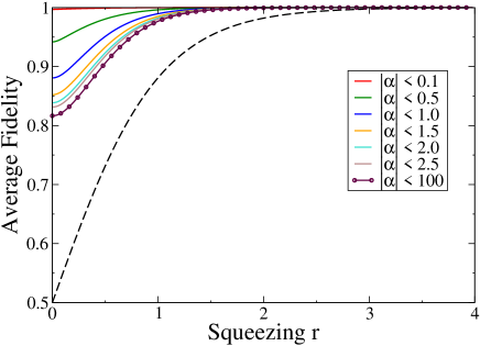
Figure 2: Solid curves give the optimal average fidelities as functions of the entanglement of the channel (squeezing $r$) for real and imaginary uniform distributions, whose ranges $R=|\alpha|$ increase from top to bottom. Dashed curve: average fidelity given by the original CVTP, which does not depend on a particular distribution. Note that for distributions covering the entire real or imaginary line ($R\rightarrow\infty$, maroon/circle curve) we still get impressive gains in efficiency when dealing with channels possessing a low degree of entanglement.

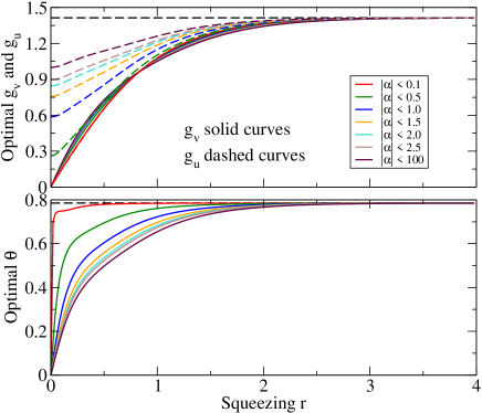
Figure 3: Parameters giving the optimal average fidelities shown in figure 2 for states lying on the real line. Note that the many curves for $g_{v}^{opt}$ are very close to each other. For $g_{u}^{opt}$ the range $R=|\alpha|$ increases from bottom to top while for $\theta$ it increases from top to bottom. The dashed black curves give the values used in the original CVTP ($g_{v}=g_{u}=\sqrt{2}\approx 1.41$ and $\theta=\pi/4\approx 0.79$). For the imaginary distribution, $g_{v}\leftrightarrow g_{u}$ and $\theta\rightarrow\pi/2-\theta$ in the graphics above.

In figure 2 we show the optimal $F_{av}^{r}(\theta,g_{v},g_{u})$ and $F_{av}^{i}(\theta,g_{v},g_{u})$ for several distributions with $|\alpha|\leq R$ as a function of the squeezing $r$ of the channel. It is worth mentioning that for $r=0$ we have no entanglement shared between Alice and Bob and the optimal values for the fidelity are the ones one would get by using only classical resources.

The first thing we note looking at figure 2 is that the optimal average fidelities are the same for the real and imaginary distributions. Second, the lower the range $R$ of the distribution the greater the efficiency. This is expected since as we decrease $R$ the states available to Alice become more and more similar. Therefore, the optimal parameters giving the best average fidelity approach the optimal parameters giving the highest fidelity for each one of the states within the distribution. Third, as we increase $R$ the optimal fidelity decreases. However, it rapidly tends to its asymptotic limit (maroon/circle line in figure 2), which is still by far superior than the fidelity given by the original CVTP (dashed line in figure 2). Figure 3 gives the optimal $\theta,g_{v}$, and $g_{u}$ leading to the optimal average fidelities shown in figure 2. Note that for low squeezing, the optimal $\theta$ is not $\pi/4$. This means that Alice needs to use an unbalanced BS to get the optimal fidelity.

We have also compared how much we gain in efficiency optimizing $F_{av}(\theta,g_{v},g_{u})$ considering $\theta,g_{v}$, and $g_{u}$ as free parameters against the optimization of $F_{av}(\pi/4,g,g)$, where only the gain $g$ is free [14, 15, 19]. As can be seen in figure 4, we obtain a considerable gain in efficiency when we allow the three parameters to be freely adjusted for a given distribution when compared to the single parameter scenario. Also, we have checked that the greater $R$ the less efficient is the single parameter optimization. For not too big $R$ it approaches the original CVTP fidelity and we must resort to the three parameter optimization to get effective efficiency gains.

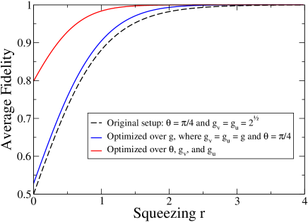
Figure 4: The curves above were calculated considering either a real or imaginary uniform distribution with $|\alpha|\leq R=5.0$. It is clear from the figure that to get an expressive gain in efficiency for quantum channels with low degree of entanglement it is crucial to optimize the average fidelity over the three free parameters.

3.2 States lying on a circumference or a disk

For a set of states $|\alpha\rangle$ available to Alice having the same amplitude $|\alpha|=R$ and phases $\omega$ given by a uniform distribution, where $0\leq\omega<2\pi$, we have in the complex plane representation of $|\alpha\rangle$ a circumference of radius $R$ centered in the vacuum. Such states with fixed magnitude and phases randomly chosen are used in the encoding of random keys in quantum cryptography based on CV states [20, 21, 22, 23, 24, 25, 26, 27, 28, 29, 30]. The determination of the optimal settings for the teleportation of such states is important since one can use the CVTP instead of the direct sending of those states from Alice to Bob in order to generate a secrete key.

The probability distribution representing such states can be written as

$$P_{c}(\alpha)=\delta(|\alpha|-R)/(2\pi R)$$ (30)

and inserting equation (30) into (16) leads to

$$F_{av}^{c}(\theta,g_{v},g_{u})=\frac{e^{-h_{+}(\theta,g_{v},g_{u})R^{2}}I_{0}[h_{-}(\theta,g_{v},g_{u})R^{2}]}{\sqrt{f_{2}(\theta,g_{v})f_{2}(\theta-\pi/2,g_{u})}}.$$ (31)

Here

$$h_{\pm}(\theta,g_{v},g_{u})=\left(\frac{f_{1}(\theta+\pi/2,g_{u})}{2f_{2}(\theta-\pi/2,g_{u})}\pm\frac{f_{1}(\theta,g_{v})}{2f_{2}(\theta,g_{v})}\right)$$ (32)

and $I_{0}[x]$ is the modified Bessel function of the first kind, i.e, the solution to $x^{2}I_{n}^{\prime\prime}[x]+xI_{n}^{\prime}[x]-(x^{2}+n^{2})I_{n}[x]=0$ with $n=0$ and boundary conditions $I_{0}[0]=1$ and $\lim_{x\rightarrow\pm\infty}I_{0}[x]\rightarrow\infty$.

The existence of the Bessel function makes the analytic solution of the optimization problem unfeasible. However, we have numerically checked for many random combinations of $r$ and $R$ that all set of parameters $\theta,g_{v}$, and $g_{u}$ leading to the optimal average fidelity for this distribution are such that $\theta=\pi/4$ and $g_{v}=g_{u}=g$. Therefore, inserting the previous parameters into equation (31), we can recast the determination of the optimal average fidelity to a single variable optimization problem. A direct computation gives the following optimal average fidelity,

$$\mathcal{F}_{opt}^{c}(g)=\frac{2\exp\left[-\frac{\left(\sqrt{2}g-2\right)^{2}R^{2}\mbox{\scriptsize{sech}}\;r}{2\left(g^{2}+2\right)\cosh r-4\sqrt{2}g\sinh r}\right]}{(g^{2}+2)\cosh^{2}r-\sqrt{2}g\sinh(2r)},$$ (33)

where the optimal $g$ is given by solving the cubic equation

$$\sqrt{2}(e^{r}\!\sinh(2r\!)\cosh r+2R^{2})-ge^{r}\!(3\cosh(2r\!)-1)\!\cosh r$$

$$-g^{2}\sqrt{2}(R^{2}-3e^{r}\sinh r\cosh^{2}r)-g^{3}e^{r}\cosh^{3}r=0.$$

In figure 5 we plot the optimal $F_{av}^{c}(\theta,g_{v},g_{u})$, or equivalently $\mathcal{F}_{opt}^{c}(g)$, for several values of $R$ as a function of the entanglement of the channel.

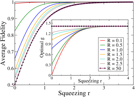
Figure 5: Solid curves are the optimal average fidelities as functions of the entanglement of the channel (squeezing $r$) for states uniformly lying on a circumference of radius $R$, with $R$ increasing from top to bottom. Inset: Optimal gain $g_{v}=g_{u}=g$ giving the optimal fidelities shown in the main graph. Here, $R$ increases from bottom to top. Dashed curves: average fidelity (main graph) and $g$ (inset) according to the original CVTP. The dashed curves are indistinguishable from the $R=50$ curves.

Looking at figure 5 we see that the smaller the radius $R$ of the distribution the greater the efficiency. Also, for $R=0$ we have $\mathcal{F}_{opt}^{c}(g)=1$ for any value of squeezing since in this case we just have one state to teleport, the vacuum state. In this scenario Bob has complete knowledge of what state will be sent and the teleportation is trivial. Now, as we increase $R$ the optimal fidelity decreases, and contrary to the pure real and imaginary distributions, it does not tend to an asymptotic limit (maroon/circle line in figure 5) yielding a better performance than that given by the original CVTP. Actually, $\mathcal{F}_{opt}^{c}(g)$ approaches the fidelity of the original CVTP.

We have also computed the optimal average fidelities assuming that both the amplitude and phase are given by independent uniform distributions, i.e., the input states are contained in a disk of radius $R$ ($|\alpha|\leq R$ and $0\leq\omega<2\pi$). In this case $P_{d}(\alpha)=\Theta(R-|\alpha|)/(\pi R^{2}).$ After a systematic numerical study for several values of squeezing $r$ and discs with radius $R$ we obtained that the optimal parameters are such that $\theta^{opt}=\pi/4$ and $g_{v}^{opt}=g_{u}^{opt}=g$, leading to the optimal average fidelity

$$\mathcal{F}_{opt}^{d}(g)=\frac{2\left(1-\exp\left[\frac{-\left(\sqrt{2}-g\right)^{2}R^{2}}{(2+g^{2})\cosh^{2}(r)-\sqrt{2}g\sinh(2r)}\right]\right)}{\left(\sqrt{2}-g\right)^{2}R^{2}}.$$ (34)

The optimal fidelity as well as the optimal settings possess the same qualitative features already explained for the distribution of states on a circumference. Quantitatively, however, we have a better performance for a given disc of radius $R$ when compared to a circumference of the same radius. This is understood noting that a disc is the union of all circumferences with radius lower than or equal to $R$. And since we have shown that the smaller $R$ the greater the fidelity for a circumference distribution, it is clear that the optimal average fidelity of a disc should outperform the optimal one for a circumference with the same $R$.

3.3 States given by Gaussian distributions

We now consider that the pool of input states with Alice is described by a Gaussian distribution with variance $1/(2\lambda)$ and mean $\beta$,

$$P_{g}(\alpha)=(\lambda/\pi)\exp{(-\lambda|\alpha-\beta|^{2})}.$$ (35)

Here, when $\beta=0$ the distribution is centered at the vacuum state and for $\beta\neq 0$ it is centered at the coherent state $|\beta\rangle$. Also, as we increase $\lambda$ (decrease the variance) the distribution approaches a single point, $\beta$, and for $\lambda\rightarrow 0$ we have a uniform distribution covering the entire complex plane.

These distributions represent what one actually gets when trying to generate a given coherent state $|\beta\rangle$. Indeed, one is never able to exactly generate a coherent state with the exact $\beta$. Rather, the generated state lies within a Gaussian distribution about the desired state, whose width depends on the quality of the coherent state generation scheme.

Inserting equation (35) into (16) we can readily compute the average fidelity for an input of coherent states distributed according to a Gaussian centered at $\beta$,

$$F_{av}^{g}(\theta,g_{v},g_{u})=\frac{\sqrt{\lambda}\exp\left[\frac{-\lambda f_{1}(\theta+\pi/2,g_{u})Re[\beta]^{2}}{f_{1}(\theta+\pi/2,g_{u})+\lambda f_{2}(\theta-\pi/2,g_{u})}\right]\sqrt{\lambda}\exp\left[\frac{-\lambda f_{1}(\theta,g_{v})Im[\beta]^{2}}{f_{1}(\theta,g_{v})+\lambda f_{2}(\theta,g_{v})}\right]}{\sqrt{f_{1}(\theta+\pi/2,g_{u})+\lambda f_{2}(\theta-\pi/2,g_{u})}\sqrt{f_{1}(\theta,g_{v})+\lambda f_{2}(\theta,g_{v})}}.$$ (36)

For Gaussians with $\beta=0$ it is not difficult to show that the optimal average fidelity is such that $\theta^{opt}=\pi/4$ and $g_{v}=g_{v}=g$, where $g$ is [14]

$$g=\frac{2\sqrt{2}+\lambda\sqrt{2}\sinh(2r)}{2+\lambda+\lambda\cosh(2r)}.$$ (37)

Note that as the Gaussian distribution variance increases, approaching a uniform distribution covering the whole complex plane ($\lambda\rightarrow 0$), equation (37) gives

$$\lim_{\lambda\rightarrow 0}g=\sqrt{2}.$$

This is exactly the value of $g$ for the original CVTP and illustrates that it is a particular case of the generalized CVTP here presented.

In figure 6 we show how the optimal average fidelity depends on the entanglement of the channel for several Gaussians with different variances. As expected, as we decrease $\lambda$, covering the entire complex plane, we recover the results of the original CVTP.

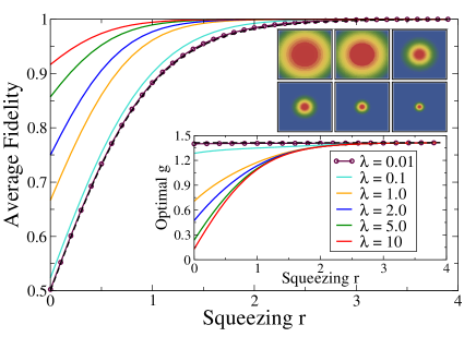
Figure 6: Solid curves give the optimal average fidelities as functions of the entanglement of the channel (squeezing $r$) for a pool of input states given by Gaussians centered at the origin with variance $1/(2\lambda)$, with $\lambda$ increasing from bottom to top. Dashed curve: average fidelity given by the original CVTP, which is indistinguishable from the corresponding one for the Gaussian with $\lambda=0.01$. Upper inset: Density plots of the several Gaussian distributions. Their variance ($\lambda$) decreases (increases) from left to right. Lower inset: The optimal gain $g_{v}=g_{u}=g$ giving the optimal fidelities shown in the main graph. Here, $\lambda$ increases from top to bottom and the dashed curve is $g$ according to the original CVTP, indistinguishable from the optimal one for the Gaussian with $\lambda=0.01$. The optimal $\theta$ is always $\pi/4$.

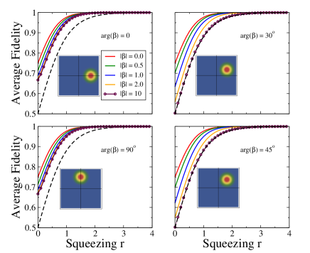
Figure 7: Optimal average fidelity as a function of the squeezing $r$ of the channel for Gaussian distributions with variance $1/(2\lambda)$, $\lambda=2.0$, and mean $\beta=|\beta|e^{\arg(\beta)}$. $|\beta|$ increases from top to bottom (solid curves) and $\arg(\beta)$ are shown in the graphics and illustrated in the insets. The dashed curve gives the fidelity of the original CVTP. For low squeezing, note that as we increase $|\beta|$ for $\arg(\beta)=0$ or $\pi/2$ (left panels) the optimal average fidelity tends to values far superior than that predicted by the original CVTP. This interesting fact does not happen if the center of the distribution moves away from the real or imaginary axis (right panels), where the curves for the original CVTP and $|\beta|=10$ fidelities cannot be distinguished.

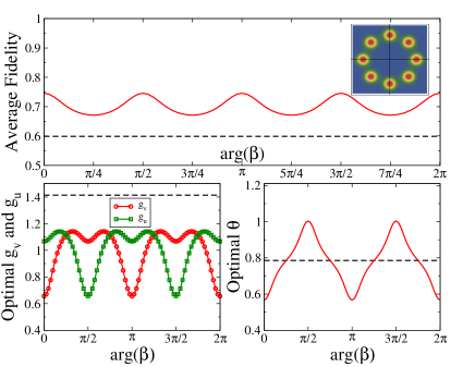
Figure 8: We show a Gaussian distribution with variance $1/(2\lambda)$, $\lambda=2.0$, and mean $\beta=|\beta|e^{\arg(\beta)}$ with $|\beta|=1.5$. The squeezing of the channel is $r=0.2$. Top panel: Optimal average fidelity as a function of $\arg(\beta)$ (solid curve). The inset shows the Gaussians with greatest (centered on the real and imaginary axis) and lowest ($\arg(\beta)=\pm 45^{o}$ and $\arg(\beta)=\pm 135^{o}$) optimal average fidelities. Left lower panel: The optimal $g_{v}$ and $g_{u}$, the values of which are in quadrature ($90^{o}$ dephasing). Note that they are only equal for $\arg(\beta)=\pm 45^{o}$ and $\arg(\beta)=\pm 135^{o}$, i.e., when $|Re(\beta)|=|Im(\beta)|$. Right lower panel: The optimal $\theta$, which equals $\theta=45^{o}$ at the same points where $g_{v}=g_{u}$. All dashed curves represent the corresponding values for the original CVTP.

If we work with Gaussian distributions displaced by $\beta\neq 0$, we cannot get a simple closed solution to the optimization problem and we must rely on numerical methods. In Figs. 7 and 8 we show numerical computations giving the optimal average fidelity and the optimal settings for Gaussians displaced in a variety of ways from the origin of the complex plane.

For the displaced Gaussians we observed that whenever $|Re[\beta]|=|Im[\beta]|$ the optimal parameters are such that $g_{v}=g_{u}$ and $\theta=\pi/4$, while $g_{v}\neq g_{u}$ and $\theta\neq\pi/4$ when $|Re[\beta]|\neq|Im[\beta]|$ (lower panels of Fig. 8). This result shows that for the great majority of the distributions here investigated the single parameter optimization strategy is not enough to achieve the highest efficiency possible. Note also that for those cases Alice must employ an unbalanced BS in order to achieve the greatest fidelity.

We have also noted that as we increase the squeezing $r$ and the width of the distribution we approach the original CVTP fidelity for distributions centered at any $\beta$. However, and quite surprising, if we displace the distribution along either the real or imaginary axis, the optimal average fidelity has an asymptotic limit as we increase $|\beta|$ considerably better than the one predicted for the original CVTP (left panels of Fig. 7). As we move the center of the distribution away from the real/imaginary axis, the asymptotic optimal average fidelity starts to approach the fidelity given by the original CVTP. For $\arg(\beta)=30^{o}$ we already have the asymptotic optimal average fidelity indistinguishable from the original CVTP fidelity (right panels of Fig. 7).

4 Discussions and Conclusion

We have extensively studied how one can modify the original continuous variable teleportation protocol [3] in order to increase its efficiency in teleporting coherent states by taking into account two facts inherently present in any actual implementation. The first one is the fact that Alice and Bob always deal with non-maximally entangled resources (finitely squeezed two-mode states) and the second one is related to the fact that Alice’s pool of possible coherent states to be teleported cannot cover the entire complex plane.

After studying several different probability distributions for the pool of input states with Alice, we showed that considerable gains in efficiency are achieved for all distributions if we introduce two slight modifications in the original setup. The first modification was the use of a beam splitter whose transmittance could be changed at our will. This beam splitter was employed to mix the state to be teleported with Alice’s share of the entangled resource, instead of the usual balanced beam splitter. The other modification was the possibility to freely choose the displacements in the quadratures, i.e., in position and momentum, of the output (teleported) state with Bob. By allowing these three actions to be independently adjusted once the entanglement of the channel and the pool of input states are known, we were able to achieve considerable gains in efficiency when compared to that predicted by the original protocol.

We have also compared the three-parameter optimization strategy against the usual one-parameter strategy, where the position and momentum gains are not independently chosen [14, 15, 19]. For certain types of distributions for the pool of input states with Alice, namely, those centered at the vacuum state and with circular symmetry, we have shown that the three-parameter strategy reduces to the one-parameter case. However, when the circular symmetry is broken, the three-parameter strategy is crucial in order to get a more efficient teleportation protocol. Indeed, we have shown that for circular symmetry broken distributions, the one-parameter strategy does not give significant gains in efficiency when compared to the original teleportation protocol while the three-parameter strategy gives considerable gains.

In addition to important gains in efficiency with the three-parameter strategy, we were also able to identify an interesting feature for distributions off-centered from the origin of the complex plane but with the circular symmetry point lying on either the real or imaginary axis. We have shown that these distributions achieve the highest gain in performance when compared to the equivalent distributions with symmetry points centered away from the real and imaginary axis. Also, for distributions with circular symmetry points lying on the real and imaginary axis, we have shown that as we increase the distance of the circular symmetry point from the origin, the optimal efficiency tends to a limiting value that is greater than the efficiency of the original teleportation protocol. This effect is more expressive for channels with a low degree of entanglement and is absent for distributions with the symmetry point not belonging to the real and imaginary axis. We believe these interesting properties might be useful in the implementation of continuous variable quantum key distribution schemes based on coherent states [20, 21, 22, 23, 24, 25, 26, 27, 28, 29, 30], where instead of transmitting the coherent state between the parties involved in the key distribution scheme, with the transmission process adding noise and degrading the signal, one teleports it using the optimal strategy here presented.

Furthermore, the calculations we made assumed a two-mode vacuum squeezed state as our entanglement resource and a pool of input states given by coherent states. These choices were dictated by the fact that the usual resources employed in actual implementations of continuous variable teleportation are described by these states [3, 7]. However, the formalism presented in Sec. 2 is quite general and can be easily adapted to any input state and any type of quantum channel. These changes are mathematically implemented by simply substituting the input and entangled states’ expansion coefficients in the position basis, equations (1), (2), (18), and (19), with the corresponding ones for the new states.

Finally, we would like to point out to a particular extension of the research here presented that might prove fruitful. It is an extensive analysis of the three parameter optimization strategy for several pool of input states assuming that Alice and Bob share quantum channels given by mixed states. Since decoherence, noise, and attenuation drive pure entangled states to mixed ones after a sufficient exposure time, it would be interesting to investigate whether the same techniques here presented can be helpful in improving the efficiency of a continuous variable teleportation protocol that employs non pure channels.

References

- [1] C. H. Bennett et al., Phys. Rev. Lett. 70 (1993) 1895.
- [2] L. Vaidman, Phys. Rev. A 49 (1994) 1473.
- [3] S. L. Braunstein and H. J. Kimble, Phys. Rev. Lett. 80 (1998) 869.
- [4] T. C. Ralph and P. K. Lam, Phys. Rev. Lett. 81 (1998) 5668.
- [5] D. Bouwmeester et al., Nature (London) 390 (1997) 575.
- [6] D. Boschi et al., Phys. Rev. Lett. 80 (1998) 1121.
- [7] A. Furusawa et al., Science 282 (1998) 706.
- [8] W. P. Bowen et al., Phys. Rev. A 67 (2003) 032302.
- [9] T. C. Zhang et al., Phys. Rev. A 67 (2003) 033802.
- [10] S. L. Braunstein and P. van Loock, Rev. Mod. Phys. 77 (2005) 513.
- [11] S. L. Braunstein, C. A. Fuchs, and H. J. Kimble, J. Mod. Opt. 47 (2000) 267.
- [12] H. Barnum, (PhD Thesis, University of New Mexico, Albuquerque, NM, USA, 1998).
- [13] L. E. Ballentine, Quantum Mechanics: A Modern Development (World Scientific, Singapore, 1998).
- [14] S. L. Braunstein, Ch. A. Fuchs, H. J. Kimble, and P. van Loock, Phys. Rev. A 64 (2001) 022321.
- [15] T. Ide, H. F. Hofmann, A. Furusawa, and T. Kobayashi, Phys. Rev. A 65 (2002) 062303.
- [16] L. Mista Jr., R. Filip, and A. Furusawa, Phys. Rev. A 82 (2010) 012322.
- [17] W. P. Bowen et al., IEEE J. Sel. Top. Quantum Electron. 9 (2003) 1519.
- [18] R. E. S. Polkinghorne and T. C. Ralph, Phys. Rev. Lett. 83 (1999) 2095.
- [19] P. van Loock and S. L. Braunstein, Phys. Rev. A 61 (1999) 010302(R).
- [20] T. C. Ralph, Phys. Rev. A 61 (1999) 010303(R).
- [21] F. Grosshans and Ph. Grangier, Phys. Rev. Lett. 88 (2002) 057902.
- [22] Ch. Silberhorn, T. C. Ralph, N. Lütkenhaus, and G. Leuchs, Phys. Rev. Lett. 89 (2002) 167901.
- [23] F. Grosshans et al., Nature (London) 421 (2003) 238.
- [24] T. Hirano et al. Phys. Rev. A 68 (2003) 042331.
- [25] R. Namiki and T. Hirano, Phys. Rev. A 67, 022308 (2003).
- [26] R. Namiki and T. Hirano, Phys. Rev. Lett. 92 (2004) 117901.
- [27] R. Namiki and T. Hirano, Phys. Rev. A 74 (2006) 032302.
- [28] D. Elser et al., New J. Phys. 11 (2009) 045014.
- [29] D. Sych and G. Leuchs, New J. Phys. 12 (2010) 053019.
- [30] P. Jouguet et al., Nature Photon. 7 (2013) 378.