Sign problem and the chiral spiral on the finite-density lattice

Abstract

We investigate the sign problem of the fermion determinant at finite baryon density in (1+1) dimensions, in which the ground state in the chiral limit should be free from the sign problem by forming a chiral spiral. To confirm it, we evaluate the fermion determinant in the continuum theory at the one-loop level and find that the determinant becomes real as expected. The conventional lattice formulation to implement a chemical potential is, however, not compatible with the spiral transformation. We discuss an alternative of the finite-density formulation and numerically verify the chiral spiral on the finite-density lattice.

Introduction

Quantum chromodynamics (QCD) has profound contents to be explored with external parameters such as the temperature $T$, the baryon chemical potential $\mu_{\text{B}}$ (that is equal to the quark chemical potential $\mu_{\text{q}}$ multiplied by the number of colors $N_{\text{c}}$), the magnetic field $B$, and so on review . The direct calculation based on QCD would be, however, feasible only in some limited ranges of these parameters. In particular along the direction of increasing $\mu_{\text{q}}$, perturbative QCD is not really useful unless the density is high enough to accommodate color superconductivity Rischke:2000cn ; Alford:2007xm . Moreover, the numerical simulation based on lattice QCD breaks down with finite $\mu_{\text{q}}$. The most serious obstacle lies in the fact that the Monte-Carlo method based on importance sampling is invalid for the finite-density case due to the complex fermion determinant, which is commonly referred to as the sign problem (see Muroya:2003qs for reviews).

The sign problem is relevant not only in the lattice-QCD simulation but also in analytical computations Dumitru:2005ng ; Fukushima:2006uv . At finite temperature, the temporal or thermal component of the gauge field $A_{4}$ plays a special role, and its expectation value is given a gauge-invariant interpretation, namely, (the phase of) the Polyakov loop, $L\equiv\mathcal{P}\exp[ig\int_{0}^{\beta}dx_{4}A_{4}]$. Because the traced Polyakov loop is an order parameter for quark deconfinement, many efforts have been devoted to the computation of the effective potential with respect to $L$ or $A_{4}$ Gross:1980br ; Weiss:1980rj ; KorthalsAltes:1993ca . With the contribution from the fermion determinant Belyaev:1991np , the effective potential at nonzero $\mu_{\text{q}}$ has turned out to take a complex value, and thus the physical meaning as a grand potential or thermal weight is obscure. This is how we can observe the sign problem even using the perturbative calculation in the continuum theory.

Since the resolution of the sign problem seems to be still far from our hands, it is very instructive to acquire some experiences with density-like effects that would cause no sign problem. Theoretical attempts along this line include the imaginary chemical potential ImaginaryChemicalPotential , the isospin chemical potential Son:2000xc , the chiral chemical potential Yamamoto:2011gk , dense QCD with two colors or with adjoint matter Muroya:2003qs ; Kogut:2000ek , the strong magnetic field $B$ D'Elia:2010nq , and so on. Among these examples the magnetic field particularly leads to a quite suggestive change in the state of quark matter. The most drastic consequences result from the Landau quantization and the dominance of the lowest Landau level for spin-$1/2$ fermions. Thus, in the strong-$B$ limit, quarks are subject to the dimensional reduction, and the transverse motion in a plane perpendicular to $B$ is frozen.

The nature of chiral symmetry breaking is affected accordingly by the strong-$B$ effects Suganuma:1990nn ; the spontaneous breaking of chiral symmetry inevitably occurs in the (1+1)-dimensional system (or in the lowest Landau level approximation Gusynin:1994re ), which is called the magnetic catalysis. This phenomenon is analogous to the superconductivity, which is also triggered by the low-dimensional nature on the Fermi surface. In chiral model studies (see Gatto:2012sp for a review) the chiral phase transition is delayed toward a higher temperature due to the magnetic catalysis, while in the finite-$T$ lattice-QCD simulation it has been recognized that the chiral crossover temperature gets smaller with increasing $B$, which is sometimes called the inverse magnetic catalysis or the magnetic inhibition Fukushima:2012kc . Another interesting example from the (1+1)-dimensional nature is the topological phenomenon such as the chiral magnetic effect Kharzeev:2007jp that might be detectable with the noncentral collision of positively charged heavy ions through charge separation or photon emission Hattori:2012je . The quickest derivation of the chiral magnetic effect makes use of the low dimensionality of the Landau zero-mode, that is, the special property of the $\gamma$ matrices; $\gamma^{5}\gamma^{\mu}=\epsilon^{\mu\nu}\gamma^{\nu}$, in (1+1) dimensions.

Such a (1+1)-dimensional system of quark matter provides us with further useful information; the ground state of the (1+1)-dimensional chiral system at finite density (with large number of internal degrees of freedom) is known to form a chiral spiral ChiralSpiral (see also deForcrand:2006zz for a lattice study). In the strong-$B$ limit, therefore, the “chiral magnetic spiral” could be one of the most likely candidates for the ground state of finite-density and magnetized quark matter Basar:2010zd . The essential idea of Basar:2010zd is that the explicit $\mu_{\text{q}}$ dependence is rotated away in (1+1) dimensions, and this procedure transforms the homogeneous chiral condensate to form a spiral in chiral basis. This at the same time implies that the sign problem should no longer be harmful once the dimensional reduction occurs.

One might have thought that the strong-$B$ limit is such a special environment having loose relevance to our realistic world. It has been argued, however, that quark matter at high density even without $B$ already exhibits a character as a pseudo-(1+1)-dimensional system locally on the Fermi surface Kojo:2009ha , just like the situation of superconductivity, and the whole Fermi surface should be covered by low-dimensional patches Kojo:2011cn . Besides, the $p$-wave pion condensation in nuclear matter having the same spiral structure is still a vital possibility beyond the normal nuclear density Tatsumi:2003fa . In this way, it is definitely worth considering the sign problem and the ground state structure in (1+1)-dimensional systems both for academic interest and for practical purpose.

Our analysis in the present work surprisingly reports that the conventional lattice formulation at finite density becomes problematic even for describing the expected ground state of such an idealized (1+1)-dimensional system. First we shall illuminate how the sign problem should be irrelevant in (1+1) dimensions by performing the perturbative calculation. Then, we will proceed to the lattice formulation to find that the conventional introduction of $\mu_{\text{q}}$ Hasenfratz:1983ba cannot realize the transformation properties in the continuum theory unless the lattice spacing is very small. We can choose an alternative that is optimal to yield a chiral spiral and conduct the numerical test to confirm a spiral formation on the lattice.

Perturbative calculation

Let us first evaluate the fermion determinant at finite $\mu_{\text{q}}$ and high enough $T$ that justifies the perturbative treatment. At the one-loop level in the deconfined phase, we should keep the Polyakov-loop $A_{4}$ background and carry out the Gaussian integration with respect to quantum fluctuations of gluons. After taking the summation over the Matsubara frequency, we can write the determinant $\mathcal{M}[A_{4}]$ (for a single flavor throughout this work) down as

$$\begin{split}&\mathcal{M}[A_{4}]=\mathcal{N}\text{e}^{-T^{d}V_{d}\Gamma[A_{4}]}=\mathcal{N}\exp\Biggl{\{}\alpha_{d}\int\frac{V_{d}d^{d}p}{(2\pi)^{d}}\\ &\qquad\text{tr}\ln\Bigl{[}\bigl{(}1\!+\!L\text{e}^{-(\varepsilon-\mu_{\text{q}})/T}\bigr{)}\bigl{(}1\!+\!L^{\dagger}\text{e}^{-(\varepsilon+\mu_{\text{q}})/T}\bigr{)}\Bigr{]}\Biggr{\}}\;,\end{split}$$ (1)

where $d$ and $V_{d}$ represent the spatial dimension and the spatial volume, respectively, and the dispersion relation is $\varepsilon=\sqrt{p^{2}+m^{2}}$. We note that the spin degeneracy factor $\alpha_{d}$ depends on $d$: $\alpha_{3}=2$ and $\alpha_{1}=1$. For practical convenience, we rotate the color basis as $ULU^{\dagger}=\text{diag}(\text{e}^{\text{i}\pi\phi_{1}},\text{e}^{\text{i}\pi\phi_{2}},\text{e}^{\text{i}\pi\phi_{3}})$, where $\phi_{1}+\phi_{2}+\phi_{3}=0$ should hold to satisfy $\det(ULU^{\dagger})=1$.

For the massless case ($m=0$), we can perform the full analytical integration for arbitrary $d$. In particular, a choice of $d=3$ immediately yields the well-known Weiss–Gross-Pisarski-Yaffe-type potential Weiss:1980rj that takes the following polynomial form review ; Belyaev:1991np ; Roberge:1986mm :

$$\Gamma[\phi]=-\frac{4\pi^{2}}{3}\sum_{i=1}^{N_{\text{c}}}B_{4}\biggl{[}\biggl{(}\frac{1+\phi_{i}}{2}\biggr{)}_{\!\!\mathrm{mod1}}-\frac{\text{i}\tilde{\mu}_{\text{q}}}{2}\biggr{]}\;,$$ (2)

where the Bernoulli polynomial appears as $B_{4}(x)=x^{2}(1-x)^{2}-1/30$ KorthalsAltes:1993ca . We also introduced the dimensionless chemical potential as $\tilde{\mu}_{\text{q}}\equiv\mu_{\text{q}}/(\pi T)$ for notational simplicity. While we choose $N_{\text{c}}=3$ in our QCD study, Eq. (2) is valid for any $\mathrm{SU}(N_{\text{c}})$ groups.

The apparent presence of the imaginary part in Eq. (2) corresponds to the sign problem. Indeed, the complex phase of the fermion determinant is nothing but $-T^{d}V_{d}\text{Im}\Gamma$ (mod $2\pi$). To gain a more informative view, we make a plot for $\text{Im}\Gamma[\phi]$ in the upper panel of Fig. 1 as a function of $\phi_{1}$ and $\phi_{2}$ (with $\phi_{3}=-\phi_{1}-\phi_{2}$). It is clear from the figure that the complex phase has a nontrivial dependence on the gauge configuration $\phi_{1}$ and $\phi_{2}$.

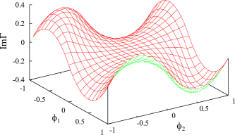
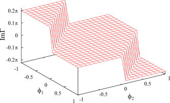
Figure 1: (Upper) Imaginary part of $\Gamma[\phi]$ for $d=3$ at $\tilde{\mu}_{\text{q}}=0.1$ shown as a function of $\phi_{1}$ and $\phi_{2}$.  (Lower) Imaginary part of $\Gamma[\phi]$ for $d=1$ at $\tilde{\mu}_{\text{q}}=0.1$.

A more interesting case is for $d=1$ corresponding to quark matter under the dimensional reduction. In this case the logarithm of the fermion determinant simplifies as

$$\Gamma[\phi]=2\pi\sum_{i=1}^{N_{\text{c}}}B_{2}\biggl{[}\biggl{(}\frac{1+\phi_{i}}{2}\biggr{)}_{\!\!\mathrm{mod1}}-\frac{\text{i}\tilde{\mu}_{\text{q}}}{2}\biggr{]}\;.$$ (3)

Here, we again used the Bernoulli polynomial as defined by $B_{2}(x)=x^{2}-x+1/6$. It is quite reasonable that $B_{4}(x)$ in Eq. (2) for $d+1=4$ is replaced with $B_{2}(x)$ in Eq. (3) for $d+1=2$. We can identify the imaginary part for $d=1$ as

$$\begin{split}\text{Im}\Gamma[\phi]&=2\pi\tilde{\mu}_{\text{q}}\sum_{i=1}^{N_{\text{c}}}\Biggl{[}\biggl{(}\frac{1+\phi_{i}}{2}\biggr{)}_{\mathrm{mod1}}-\frac{1}{2}\biggr{]}\\ &=\left\{\begin{array}[]{cp{1em}l}0&&(-1<\phi_{1}+\phi_{2}<1)\\ -2\pi\tilde{\mu}_{\text{q}}&&(\phi_{1}+\phi_{2}\geq 1)\\ +2\pi\tilde{\mu}_{\text{q}}&&(\phi_{1}+\phi_{2}\leq-1)\end{array}\right.\;.\end{split}$$ (4)

This analytic behavior is visually shown in the lower panel of Fig. 1. The step emerges when $(1+\phi_{3})/2=(1-\phi_{1}-\phi_{2})/2$ exceeds the boundary of modular one, and then, as is clear from the above expression, $\text{Im}\Gamma$ takes a constant $\pm 2\pi\tilde{\mu}_{\text{q}}$, which is $\pm 0.2\pi$ in our numerical setup ($\tilde{\mu}_{\text{q}}=0.1$) to draw Fig. 1.

With a more careful deliberation on the phase-space volume, we see that an imaginary part in the region $|\phi_{1}+\phi_{2}|\geq 1$ has no contribution since this finite value is quantized as $TV_{1}\text{Im}\Gamma=2\pi n$ with an integer $n$. To see this, let us consider the branch-cut contribution from the logarithm in the integrand of Eq. (1), which appears when the real part in the logarithm turns negative, i.e., $\mathrm{Re}[\text{e}^{\text{i}\pi\phi_{i}-(|p|-\mu_{\text{q}})/T}]<-1$. The momentum integration under this condition picks up the phase-space volume satisfying $|p|<\mu_{\text{q}}$, that is,

$$\begin{split}&\pm\int\frac{V_{1}dp}{2\pi}2\pi\,\theta(\mu_{\text{q}}-|p|)\\ \to&\pm\!\!\!\!\!\!\!\!\sum_{\text{Phase Space}}\!\!\!\!\!\!\!2\pi\,\theta(\mu_{\text{q}}-|p|)=\pm 2\cdot 2\pi\biggl{\lfloor}\frac{V_{1}\mu_{\text{q}}}{2\pi}\biggr{\rfloor}\;,\end{split}$$ (5)

where $\lfloor\cdots\rfloor$ represents the floor function. Equation (5) reproduces Eq. (4) multiplied with $TV_{1}$ in a quantized form. In summary of perturbative analyses in the (1+1)-dimensional continuum theory, as conjectured, we have actually confirmed that no sign problem arises.

Lattice formulation

This simple analytical observation is, however, not easy to be validated on the lattice, unless one reaches the continuum limit. To make the point explicitly clear, let us take a pseudo-(1+1)-dimensional system discarding two transverse (1st and 2nd) components. Then, in Euclidean space-time with the longitudinal (3rd) and the temporal (4th) components, the Lagrangian density, $\mathcal{L}_{\text{eff}}=\bar{\psi}D(\mu_{\text{q}})\psi$, with $D(\mu_{\text{q}})=\gamma^{3}(\partial_{3}-\text{i}gA_{3})+\gamma^{4}(\partial_{4}+\mu_{\text{q}}-\text{i}gA_{4})$ defines the theory. Here, we consider the most interesting case of $m=0$ only. Then, we can immediately confirm that $\mu_{\text{q}}$ is superficially erased by the following rotation:

$$\psi\;\to\;\psi=U\psi^{\prime}\;,\qquad\bar{\psi}\;\to\;\bar{\psi}=\bar{\psi}^{\prime}U\;,$$ (6)

with $U\equiv\exp\bigl{(}-\mu_{\text{q}}\gamma^{3}\gamma^{4}x_{3}\bigr{)}$. The chemical potential can be factorized out by the unitary transformation, $D(\mu_{\text{q}})=U^{\dagger}D(0)U^{\dagger}$, and thus the fermion determinant is independent of $\mu_{\text{q}}$. Strictly speaking, this rotation also causes a shift in momenta carried by $\psi^{\prime}$ and $\bar{\psi}^{\prime}$, and such a shift gives rise to nontrivial $\mu_{\text{q}}$ dependence through chiral anomaly ChiralSpiral . For the moment, it suffices for our purpose of seeing the spiral if we focus on the tree-level elimination of the $\mu_{\text{q}}$-term, and we will not go into anomalous $\mu_{\text{q}}$ dependence.

In the conventional lattice formulation Hasenfratz:1983ba , $\mu_{\text{q}}$ is introduced as

$$\begin{split}&\bar{\psi}\gamma^{4}(\partial_{4}+\mu_{\text{q}})\psi=(\bar{\psi}\,\text{e}^{-\mu_{\text{q}}x_{4}})\gamma^{4}\partial_{4}(\text{e}^{\mu_{\text{q}}x_{4}}\psi)\\ &\simeq\frac{1}{2}\bar{\psi}(x)\gamma^{4}\text{e}^{\mu_{\text{q}}}\psi(x+\hat{4})-\frac{1}{2}\bar{\psi}(x)\gamma^{4}\text{e}^{-\mu_{\text{q}}}\psi(x-\hat{4})\;.\end{split}$$ (7)

If we apply the transformation with Eq. (6) on the lattice version of the Lagrangian, we can find $UD(\mu_{\text{q}})U$ as

$$\frac{1}{2}\biggl{\{}\bar{\psi}^{\prime}(x)\Bigl{[}(\gamma^{3}\cos\mu_{\text{q}}\!-\!\gamma^{4}\sin\mu_{\text{q}})\psi^{\prime}(x\!+\!\hat{3})\!+\!\gamma^{4}\text{e}^{\mu_{\text{q}}}\psi^{\prime}(x\!+\!\hat{4})\Bigr{]}$$

$$-\bar{\psi}^{\prime}(x)\Bigl{[}(\gamma^{3}\cos\mu_{\text{q}}\!+\!\gamma^{4}\sin\mu_{\text{q}})\psi^{\prime}(x\!-\!\hat{3})\!+\!\gamma^{4}\text{e}^{-\mu_{\text{q}}}\psi^{\prime}(x\!-\!\hat{4})\Bigr{]}\biggr{\}}$$ (8)

apart from the link variables. In the continuum limit (i.e. the lattice spacing $a\to 0$), where $\mu_{\text{q}}a$ goes vanishingly small, the explicit $\mu_{\text{q}}$ dependence certainly disappears as anticipated from the continuum theory. In this sense, such an incomplete cancellation in Eq. (7) is a lattice artifact, and yet, this is crucial for the sign problem and the formation of chiral spiral.

One quick remedy for the noncancellation problem is to alter the way to formulate $\mu_{\text{q}}$ on the lattice. We shall propose to introduce the chemical potential as $D(\mu_{\text{q}})=U^{{\dagger}}D(0)U^{{\dagger}}$, i.e. (see Creutz:2010cz for a similar proposal),

$$\bar{\psi}\bigl{(}\gamma^{3}\partial_{3}+\gamma^{4}\mu_{\text{q}}\bigr{)}\psi=(\bar{\psi}\,U^{\dagger})\gamma^{3}\partial_{3}(U^{\dagger}\psi)$$

$$\simeq\frac{1}{2}\bar{\psi}(x)\bigl{(}\gamma^{3}\cos\mu_{\text{q}}+\gamma^{4}\sin\mu_{\text{q}}\bigr{)}\psi(x+\hat{3})$$

$$\quad-\frac{1}{2}\bar{\psi}(x)\bigl{(}\gamma^{3}\cos\mu_{\text{q}}-\gamma^{4}\sin\mu_{\text{q}}\bigr{)}\psi(x-\hat{3})$$ (9)

(with link variables omitted). In this form, it may look trivial at glance that the rotation with Eq. (6) can get rid of the $\mu_{\text{q}}$ dependence. The situation is not such trivial, though. One can actually prove that the eigenvalues of this fermion operator appear as a quartet: $\lambda$, $-\lambda$, $\lambda^{\ast}$, and $-\lambda^{\ast}$. In other words, the fermion determinant is always real regardless of the dimensionality! Needless to say, this cannot be a resolution of the sign problem. Because $\sin\mu_{\text{q}}$ is accompanied by $\cos q_{3}$ in momentum space of Eq. (9), the sign of $\mu_{\text{q}}$ changes for the fermion doublers in the $\hat{3}$ direction. Therefore, if we interpret the doublers as different quark flavors, $\mu_{\text{q}}$ as put in Eq. (9) represents the isospin chemical potential rather than the quark chemical potential, so that the determinant is always real! This also means that the new formulation as in Eq. (9) cannot produce a chiral spiral.

Thus, we must cope with the doubler problem to treat $\mu_{\text{q}}$ as a quark chemical potential. In this work we shall naïvely add the Wilson term, $r_{W}\bar{\psi}\partial^{2}\psi$ (where we choose $r_{W}=1$) to make heavy doublers decouple from the dynamics. Not to violate the transformation properties, $D(\mu_{\text{q}})=U^{\dagger}D(0)U^{\dagger}$, we must implement the Wilson term according to Eq. (9) as $r_{W}\bar{\psi}\partial^{2}\psi\rightarrow r_{W}(\bar{\psi}U^{\dagger})\partial^{2}(U^{\dagger}\psi)$. In this case the fermion determinant becomes real only for discrete values of $\mu_{\text{q}}$, that is quantized as $\mu_{\text{q}}=(\pi/N)n$, where $N$ is the number of lattice sites along the $x_{3}$ direction. Because the Wilson term has an explicit $x_{3}$ dependence, we must require $\text{e}^{2\mu_{\text{q}}\gamma^{3}\gamma^{4}N}=1$ to keep the action invariant under the shift: $x_{3}\to x_{3}+N$.

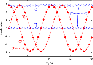
Figure 2: Condensates $\sigma$ and $\eta$ at $\mu_{\text{q}}=2\pi/N$ (with $N=32$) as a function of $x_{3}$ in the lattice unit. The closed circle and triangle dots represent the results from our new formulation, while the open circle and triangle dots from the conventional one. The solid curves are $2.86\cos[2\mu_{\text{q}}(x_{3}-1)]$ and $2.86\sin[2\mu_{\text{q}}(x_{3}-1)]$ that fit the oscillation behavior.

For $\mu_{\text{q}}=(\pi/N)n$, the determinant returns to a real value. While the bulk properties are fixed by the whole quantity of the determinant, we emphasize here, the microscopic dynamics is far more nontrivial. If the vacuum at $\mu_{\text{q}}=0$ has a nonzero and homogeneous chiral condensate $\sigma_{0}\equiv\langle\bar{\psi}\psi\rangle\neq 0$, the rotated vacuum with Eq. (6) at $\mu_{\text{q}}\neq 0$ should yield $\sigma_{0}=\langle\bar{\psi}^{\prime}\psi^{\prime}\rangle$ as well. In terms of the original basis, accordingly, we can expect $\sigma\equiv\langle\bar{\psi}\psi\rangle=\sigma_{0}\cos(2\mu_{\text{q}}x_{3})$ and $\eta\equiv\langle\bar{\psi}\gamma^{3}\gamma^{4}\psi\rangle=\sigma_{0}\sin(2\mu_{\text{q}}x_{3})$, which locally breaks chiral symmetry but does not globally, i.e., the average of the condensate vanishes: $\int d^{2}x\langle\bar{\psi}\psi\rangle=0$.

In Fig. 2 we show the condensates as a function of $x_{3}$ defined by $\sigma(x_{3})\equiv N_{t}^{-1}\sum_{x_{4}}\text{tr}[D^{-1}(\mu_{\text{q}})]$ and $\eta(x_{3})\equiv N_{t}^{-1}\sum_{x_{4}}\text{tr}[\gamma^{3}\gamma^{4}D^{-1}(\mu_{\text{q}})]$ (in the lattice unit). This is the result for one gauge configuration generated after 1000 quench updates using the Wilson gauge action with $\beta=5.0$. If we use the conventional introduction of $\mu_{\text{q}}$ as in Eq. (7), only $\sigma$ has a finite expectation value and the oscillatory pattern is hardly visible. With the new formulation as in Eq. (9), on the other hand, both $\sigma$ and $\eta$ take a finite value to develop a clear chiral spiral. [One should be careful to interpret this result: The exact chiral limit with strict (1+1) dimensions gives rise to no chiral condensate. This is why we set our problem in pseudo-(1+1) dimensions and also the Wilson term plays a role.]

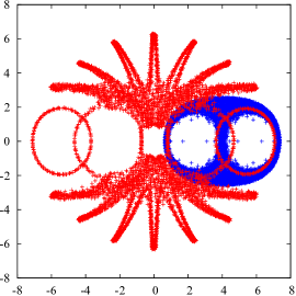
Figure 3: Eigenvalue distribution of the finite-$\mu_{\text{q}}$ fermion operator on the $32\times 32$ lattice ($N=32$) for the gauge configuration corresponding to Fig. 2. Results with $\mu_{\text{q}}=2\pi/N$ (red dots) overlaid on those with $\mu_{\text{q}}=0$ (blue dots).

Since the chiral condensate is related to the low-lying eigenvalues via the Banks-Casher relation, it is interesting to see how the eigenvalue distribution changes with the chiral spiral. The Wilson term breaks anti-Hermiticity, and the eigenvalues are complex even at $\mu_{\text{q}}=0$, so that the original Banks-Casher relation needs a modification; the chiral condensate should be derived from the eigenvalues of $D^{\dagger}(0)D(0)$ rather than $D(0)$ Giusti:2008vb . In this work, we do not calculate the former, and yet, it is quite interesting to investigate the qualitative changes of the latter at finite $\mu_{\text{q}}$, which is presented in Fig. 3.

Figure 3 shows the eigenvalue distribution of $D(\mu_{\text{q}})$ for $\mu_{\text{q}}=0$ (blue dots) and $\mu_{\text{q}}=2\pi/N$ (red dots) as introduced in Eq. (9). At $\mu_{\text{q}}=0$ the eigenvalue distribution is just the same as a conventional one. With increasing $\mu_{\text{q}}$ the distribution spreads to the negative real region, and when $\mu_{\text{q}}$ reaches a multiple of $\pi/N$, the determinant should be identical to the $\mu_{\text{q}}=0$ value, though the eigenvalue distribution looks totally different. Although the distribution appears to be symmetric for $\mu_{\text{q}}=(2\pi/N)n$ as seen in Fig. 3, there is no longer a quartet structure nor any pairwise symmetry. It is miraculous that the product of all these eigenvalues happens to be real.

Conclusions

We have justified the idea that the sign problem of the fermion determinant at finite $\mu_{\text{q}}$ be irrelevant in the (1+1)-dimensional system. This is caused by the chiral transformation that removes the chemical potential. We have first evaluated the determinant perturbatively in the continuum theory, and found that the imaginary part in the (1+1)-dimensional case vanishes unlike the (3+1)-dimensional situation that suffers from the sign problem.

For the discretized fermion on the (1+1)-dimensional lattice, the conventional way to impose a chemical potential causes the sign problem, which is a lattice artifact and should be absent in the continuum limit. In practice, however, this lattice artifact severely hinders the formation of the chiral spiral. To evade this problem, we have proposed a new method to introduce a chemical potential by twisting the Dirac operator along one of the spatial directions by $\exp(\mu_{\text{q}}\gamma_{3}\gamma_{4}x_{3})$, which recovers the correct continuum limit as it should. In this case, the fermion determinant becomes real, but it turns out that such a chemical potential induces not a quark density but a doubler (or isospin) density if the doublers are not killed. We then find no chiral spiral. By diminishing spurious symmetry with doublers, we have successfully confirmed a clear chiral spiral. The eigenvalues of our fermion operator has a peculiar distribution structure, which suggests some relation between the appearance of some distribution pattern and the formation of the chiral spiral, which we leave for a future problem.

Our idea of the spatially twisted chemical potential can be applied to not only (1+1) dimensions but also more general dimensions. If the spiral structure is the genuine ground state at strong magnetic field or at high baryon density that brings about the dimensional reduction, the conventional formulation with $\mu_{\text{q}}$ is not really an optimal choice. The present work has manifestly demonstrated the advantage of the new formulation to investigate the sign problem and the chiral spiral. It is also an intriguing future problem to study our method using the other fermions, particularly the overlap fermion that also exhibits a peculiar distribution of finite-density eigenvalues Bloch:2006cd .

- (1) K. Fukushima and T. Hatsuda, Rept. Prog. Phys. 74, 014001 (2011); K. Fukushima, J. Phys. G 39, 013101 (2012); K. Fukushima and C. Sasaki, Prog. Part. Nucl. Phys. 72, 99 (2013).
- (2) D. H. Rischke, D. T. Son and M. A. Stephanov, Phys. Rev. Lett. 87, 062001 (2001).
- (3) M. G. Alford, A. Schmitt, K. Rajagopal and T. Schaefer, Rev. Mod. Phys. 80, 1455 (2008).
- (4) S. Muroya, A. Nakamura, C. Nonaka and T. Takaishi, Prog. Theor. Phys. 110, 615 (2003); G. Aarts, PoS LATTICE 2012, 017 (2012).
- (5) A. Dumitru, R. D. Pisarski and D. Zschiesche, Phys. Rev. D 72, 065008 (2005).
- (6) K. Fukushima and Y. Hidaka, Phys. Rev. D 75, 036002 (2007).
- (7) D. J. Gross, R. D. Pisarski and L. G. Yaffe, Rev. Mod. Phys. 53, 43 (1981).
- (8) N. Weiss, Phys. Rev. D 24, 475 (1981); Phys. Rev. D 25, 2667 (1982); K. Enqvist and K. Kajantie, Z. Phys. C 47, 291 (1990); V. M. Belyaev, Phys. Lett. B 241, 91 (1990); Phys. Lett. B 254, 153 (1991).
- (9) C. P. Korthals Altes, Nucl. Phys. B 420, 637 (1994).
- (10) V. M. Belyaev, I. I. Kogan, G. W. Semenoff and N. Weiss, Phys. Lett. B 277, 331 (1992).
- (11) M. G. Alford, A. Kapustin and F. Wilczek, Phys. Rev. D 59, 054502 (1999); P. de Forcrand and O. Philipsen, Nucl. Phys. B 642, 290 (2002); M. D’Elia and M. -P. Lombardo, Phys. Rev. D 67, 014505 (2003).
- (12) D. T. Son and M. A. Stephanov, Phys. Rev. Lett. 86, 592 (2001); J. B. Kogut and D. K. Sinclair, Phys. Rev. D 66, 034505 (2002).
- (13) A. Yamamoto, Phys. Rev. Lett. 107, 031601 (2011); Phys. Rev. D 84, 114504 (2011).
- (14) J. B. Kogut, M. A. Stephanov, D. Toublan, J. J. M. Verbaarschot and A. Zhitnitsky, Nucl. Phys. B 582, 477 (2000).
- (15) M. D’Elia, S. Mukherjee and F. Sanfilippo, Phys. Rev. D 82, 051501 (2010); G. S. Bali, F. Bruckmann, G. Endrodi, Z. Fodor, S. D. Katz, S. Krieg, A. Schafer and K. K. Szabo, JHEP 1202, 044 (2012); G. S. Bali, F. Bruckmann, G. Endrodi, Z. Fodor, S. D. Katz and A. Schafer, Phys. Rev. D 86, 071502 (2012).
- (16) H. Suganuma and T. Tatsumi, Annals Phys. 208, 470 (1991); K. G. Klimenko, Theor. Math. Phys. 89, 1161 (1992) [Teor. Mat. Fiz. 89, 211 (1991)]; Z. Phys. C 54, 323 (1992).
- (17) V. P. Gusynin, V. A. Miransky and I. A. Shovkovy, Phys. Rev. Lett. 73, 3499 (1994); Phys. Rev. D 52, 4718 (1995); I. A. Shushpanov and A. V. Smilga, Phys. Lett. B 402, 351 (1997); K. Fukushima and J. M. Pawlowski, Phys. Rev. D 86, 076013 (2012).
- (18) R. Gatto and M. Ruggieri, Lect. Notes Phys. 871, 87 (2013).
- (19) K. Fukushima and Y. Hidaka, Phys. Rev. Lett. 110, 031601 (2013).
- (20) D. E. Kharzeev, L. D. McLerran and H. J. Warringa, Nucl. Phys. A 803, 227 (2008); K. Fukushima, D. E. Kharzeev and H. J. Warringa, Phys. Rev. D 78, 074033 (2008).
- (21) K. Hattori and K. Itakura, Annals Phys. 330, 23 (2013); Annals Phys. 334, 58 (2013); G. Basar, D. Kharzeev, D. Kharzeev and V. Skokov, Phys. Rev. Lett. 109, 202303 (2012); K. Fukushima and K. Mameda, Phys. Rev. D 86, 071501 (2012).
- (22) B. -Y. Park, M. Rho, A. Wirzba and I. Zahed, Phys. Rev. D 62, 034015 (2000); V. Schon and M. Thies, “2-D model field theories at finite temperature and density,” In M. Shifman (ed.): At the frontier of particle physics, vol. 3 1945-2032; B. Bringoltz, Phys. Rev. D 79, 125006 (2009).
- (23) P. de Forcrand and U. Wenger, PoS LAT 2006, 152 (2006) [hep-lat/0610117].
- (24) G. Basar, G. V. Dunne and D. E. Kharzeev, Phys. Rev. Lett. 104, 232301 (2010); E. J. Ferrer, V. de la Incera and A. Sanchez, Acta Phys. Polon. Supp. 5, 679 (2012).
- (25) T. Kojo, Y. Hidaka, L. McLerran and R. D. Pisarski, Nucl. Phys. A 843, 37 (2010).
- (26) T. Kojo, Y. Hidaka, K. Fukushima, L. D. McLerran and R. D. Pisarski, Nucl. Phys. A 875, 94 (2012).
- (27) T. Tatsumi, nucl-th/0302009.
- (28) P. Hasenfratz and F. Karsch, Phys. Lett. B 125, 308 (1983).
- (29) M. Creutz and T. Misumi, Phys. Rev. D 82, 074502 (2010); T. Misumi, JHEP 1208, 068 (2012).
- (30) A. Roberge and N. Weiss, Nucl. Phys. B 275, 734 (1986).
- (31) L. Giusti and M. Luscher, JHEP 0903, 013 (2009).
- (32) J. C. R. Bloch and T. Wettig, Phys. Rev. Lett. 97, 012003 (2006).