Numerical multi-loop calculations with SecDec

Abstract

The new version 2.1 of the program SecDec is described, which can be used for the factorisation of poles and subsequent numerical evaluation of multi-loop integrals, in particular massive two-loop integrals. The program is not restricted to scalar master integrals; more general parametric integrals can also be treated in an automated way.

1 Introduction

In the absence of smoking gun signals of New Physics at the LHC so far, precision measurements play a crucial role in the search for less direct signs of New Physics and in exploring the Higgs sector. Certainly this is only possible if precise theory predictions are available. In most cases, this means that next-to-leading order (NLO) calculations are necessary, ideally matched to a parton shower. However, there is a number of examples where NNLO precision is required. While in the case of jet production the main challenge at NNLO consists in the treatment of the doubly unresolved real radiation part, processes involving massive particles – e.g. top quarks or $W/Z$ bosons – contain another bottleneck, given by the two-loop integrals entering the virtual corrections. The recent result for $t\bar{t}$ production at NNLO [1] is based on a semi-numerical representation of the integrals [2], while fully analytical representations for most of the master integrals needed for this process have been worked out in [3, 4, 5, 6, 7]. Planar two-loop master integrals entering the production of two massive vector bosons at NNLO have been calculated in [8], and in the high energy limit in [9] for the case of $W$ pair production.

However, non-planar massive two-loop integrals which cannot be expressed entirely in terms of generalized harmonic polylogarithms still pose a problem for a fully analytical evaluation. Numerical methods on the other hand do not have these difficulties. For the latter the problem rather lies in the isolation of the singularities, as well as in numerical efficiency and accuracy.

The program SecDec, presented in [10, 11], performs the task of isolating singularities which, if regulated by dimensional regularisation, appear as poles in $1/\epsilon$, in an automated way, based on the algorithm of sector decomposition [12, 13, 14]. Other implementations of sector decomposition into public programs are also available [15, 16, 17]. However, the latter are more or less restricted to the Euclidean region, while SecDec can deal with physical kinematics.

In this talk the new features of the program SecDec 2.1 will be presented, along with some results.

2 Structure, usage and new features of SecDec version 2.1

2.1 Structure

As can be seen from Fig. 1, the program contains two sections, one for loop integrals, one for more general parametric functions (corresponding to the directories loop and general). The loop part has been extended in version 2.1 to be able to treat parametric integrals which are not in the canonical form as obtained directly from standard Feynman parametrisation. They can have a different format coming for example from variable transformations and/or analytical integrations over some Feynman parameters. Hence, as these functions differ from the standard representation which the program would derive from the propagators in an automated way, they have to be defined in an input file by the user. The detailed syntax to define these functions is given in subsection 2.4.1. Contour deformation is available for these functions, as they are assumed to originate from a Feynman integral structure where poles on the real axis are protected by the infinitesimal $i\delta$ prescription.

The part in the directory general can deal with even more general parametric functions, where the integrand can consist of a product of arbitrary length of polynomial functions to some power. However, these functions should have only endpoint singularities (i.e. dimensionally regulated singularities at the integration boundaries). Contour deformation is not available in this case because the correct sign of the imaginary part steering the deformation into the complex plane cannot be inferred if the assumption of an underlying loop integral structure is dropped.

The procedure of iterated sector decomposition and subsequent treatment is the same for all the different types of input functions, and is described in [10, 11].

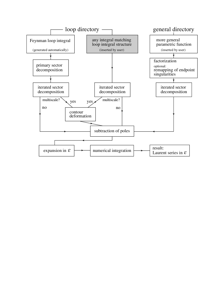
Figure 1: Flowchart showing the structure of the program SecDec.

2.2 Installation

The current version of the program can be downloaded from
http://projects.hepforge.org/secdec.

Unpacking the tar archive via tar xzvf SecDec-2.1.2.tar.gz will create a directory called SecDec-2.1.2. Changing to the SecDec-2.1.2 directory and running ./install will compile the Cuba library [18] needed for the numerical integration.

Prerequisites are Mathematica, version 6 or above, Perl (installed by default on most Unix/Linux systems) and a C++ compiler. If the Fortran option is used, a Fortran compiler is obviously also required.

2.3 Usage

There are two files to be edited: a text file param*.input where the parameters are set, and a Mathematica file template*.m where the funtion(s) to be integrated are defined. In more detail:

1. In the loop directory, edit the files paramloop.input and templateloop.m if you want to compute a Feynman loop integral in a fully automated way. If you would like to define a set of own functions rather than a standard loop integral, take the files paramuserdefined.input and templateuserdefined.m as a starting point. In the general directory, the analogous files are param.input and template.m.

   Let us call the files edited by the user myparamfile.input and mytemplatefile.m.

2. Execute the command ./launch -p myparamfile.input -t mytemplatefile.m in the shell. If you add the option -u in the loop directory, user defined functions are computed.
   If your files myparamfile.input, mytemplatefile.m are in a different directory, say, myworkingdir, use the option -d myworkingdir, i.e. the full command then looks like ./launch -d myworkingdir -p myparamfile.input -t mytemplatefile.m, executed from the directory SecDec/loop or SecDec/general.

3. Collect the results. Depending on whether you have used a single machine or submitted the jobs to a cluster, the following actions will be performed:

   • If the calculations are done sequentially on a single machine, the results will be collected automatically (via the corresponding results*.pl called by launch). The output file will be displayed with your specified text editor.

   • If the jobs have been submitted to a cluster, when all jobs have finished, execute the command ./results.pl [-d myworkingdir -p myparamfile] in the general, and ./resultsloop.pl [-d myworkingdir -p myparamfile] or ./resultsuserdefined.pl [-d myworkingdir -p myparamfile] in the loop directory, respectively. This will create the files containing the final results in the graph subdirectory specified in the input file.

4. After the calculation and the collection of the results is completed, you can use the shell command ./launchclean[graph] to remove obsolete files.

More details about the usage can be found in Ref. [19], and also in the documentation coming with the program.

2.4 New Features

Version 2.1 of SecDec contains the following new features, also partially illustrated by examples in Section 3.

2.4.1 Evaluation of user-defined functions in the loop part:

If the user would like to calculate a “standard” loop integral, it is sufficient to specify the propagators, and the program will construct the integrand in terms of Feynman parameters automatically. However, analytical manipulations on the integrand before starting the iterated sctor decomposition can be helpful when dealing with complicated integrals. For example, integrating out one Feynman parameter analytically reduces the number of integration variables for the subsequent Monte Carlo integration and therefore can improve numerical efficiency. This implies that the constraint $\delta(1-\sum_{i}x_{i})$ has been used already to achieve a convenient parametrisation, and therefore no primary sector decomposition to eliminate the $\delta$-constraint is needed anymore. In such a case, the user can skip the primary sector decomposition step and insert the integrand functions directly into the Mathematica input file.

The detailed syntax is as follows. The user-defined functions should be polynomial in the Feynman parameters and can also involve kinematic invariants, i.e. should be structurally similar to the functions of type $\mathcal{U}$ and $\mathcal{F}$ (see e.g. eq. (3.1)). They can be raised to some power which does not have to be an integer. These functions in addition can be multiplied by an arbitrary “numerator” function. The only condition the latter must fulfill is that it should not contain any singularities or thresholds. In case the functions $\mathcal{U}$ and $\mathcal{F}$ contain thresholds, a deformation of the integration contour into the complex plane will be performed. The setup is such that the integration contour will be formed based on the function $\mathcal{F}$. The list of user-defined functions must be inserted into mytemplatefile.m using the following syntax
functionlist={function_1,function_2,…,function_i,…};
with function_i={# of function,{list of exponents},{{function $\mathcal{U}$, exponent of $\mathcal{U}$, decomposition flag},{function $\mathcal{F}$,exponent of $\mathcal{F}$,decomposition flag}}, numerator}.
The # of function is an integer labelling the function, where the default is sequential numbering.

Each entry in the comma separated list of exponents corresponds to an exponent of a Feynman parameter occurring as a monomial in the Feynman integral. The decomposition flag should be A if no iterated sector decomposition is desired, and B if the function needs further decomposition. The numerator may contain several functions, with different exponents, as long as the functions are non-singular. An example including detailed comments can be found in /loop/templateuserdefined.m and /loop/paramuserdefined.input.

2.4.2 Tensor integrals:

For the computation of tensor integrals, where the tensor is contracted with external momenta and/or loop momenta, the construction of the Feynman integral via topological cuts needs to be switched off, which corresponds to cutconstruct=0.
To define the numerator in mytemplatefile.m, each scalar product of loop momenta contracted with either external momenta or loop momenta should be given as an entry of a list:
numerator={prefactor,comma separated list of scalar products}. For example, a numerator of the form $2\,(k_{1}\cdot p_{1})(k_{1}\cdot k_{2})$, where $p_{1}$ is an external momentum and the $k_{i}$ are loop momenta, should be given as numerator={2, $k1*p1$, $k1*k2$ }.

2.4.3 Error estimates:

When dealing with complicated integrands it can happen that the error given by the Monte Carlo integration program – which is based on the number of sampling points only – underestimates the true error. The numerical integrators contained in the Cuba library [18, 20] give an estimate how trustworthy the stated error is. The new SecDec version 2.1 collects the maximal error probability for each computed order in the Laurent series in $\epsilon$ and writes it to the result files *.res. In the generic case, the information on the reliability of the stated error is given as a probability with values between 0 and 1. If the integrator returns a value larger than one, the integration has not come to successful completion, and a warning is written to the result files. This feature should enable the user to assess the reliability of the numerical result, respectively the given error estimate.

3 Examples and Results

3.1 Non-planar massive two-loop diagrams entering NNLO $t\bar{t}$ production

The sector decomposition algorithm is described in detail in [12, 21], while the general structure of the program SecDec is described in [10, 11]. Therefore we concentrate mainly on the new features and results here.

The most complicated master topologies occurring in the two-loop corrections to $t\bar{t}$ production in the $gg$ channel are the non-planar seven-propagator integrals shown in Fig.2.

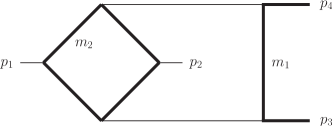
(a) ggtt1

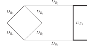
(b) ggtt2

Figure 2: Massive non-planar two-loop box diagrams entering the heavy (a) and light (b) fermionic correction to the $gg\to t\bar{t}$ channel; the bold lines denote massive particles.

Analytic results for the integral containing a sub-diagram with a massive loop (called ggtt1 here), are not available, while analytic results for the diagram corresponding to massless fermionic corrections in a sub-loop (called ggtt2 here) have become available only very recently [3]. However, the numerical evaluation of ggtt1 with SecDec is much easier than the one of ggtt2, due to its less complicated infrared singularity structure. While the leading poles of ggtt2 are of order $1/\epsilon^{4}$, and intermediate expressions during sector decomposition contain (spurious) poles where the degree of divergence is higher than logarithmic, the integral ggtt1 is finite and free from spurious poles. Therefore we can evaluate ggtt1 with SecDec 2.1 using the fully automated setup. In contrast, for ggtt2 it turned out to be advantageous to make some analytical manipulations beforehand. In particular, it was useful to perform one parameter integration analytically before feeding the integral into the decomposition and numerical integration algorithm. Further, we introduced special transformations to reduce the occurrence of spurious singularities, which are described in detail in [19]. These manipulations lead to functions which were not in the “standard form” of Feynman parameterised loop integrals anymore. Therefore this entailed the development of a setup for “non-standard” parametric functions, which has been made available for the user as described in section 2.4.1, as it can be beneficial in other contexts as well.

The expression for the scalar integral ggtt2 in momentum space is given by

$$\mathcal{G}_{ggtt2}=\left(\frac{1}{\mathrm{i}\pi^{\frac{\mathrm{D}}{2}}}\right)^{2}\int\frac{\mathrm{d^{D}}k_{1}\,\,\mathrm{d^{D}}k_{2}}{D_{R_{1}}D_{R_{2}}D_{R_{3}}D_{R_{4}}D_{B_{1}}D_{B_{2}}D_{B_{3}}}$$ (1)

where $\mathrm{D}=4-2\epsilon$. Integrating out the loop momentum $k_{2}$ (corresponding to massless sub-loop) first, we are left with an expression containing $k_{1}$ and external momenta only:

$$\mathcal{I}_{R}=\frac{1}{\mathrm{i}\pi^{\mathrm{D}/2}}\int\frac{\mathrm{d^{D}}k_{2}}{D_{R_{1}}D_{R_{2}}D_{R_{3}}D_{R_{4}}}=\Gamma(2+\epsilon)\int\prod_{i=1}^{4}\mathrm{d}x_{i}\delta(1-\sum_{j=1}^{4}x_{j})\mathcal{F}(\vec{x},k_{1})^{-2-\epsilon}\text{ ,}$$ (2)

with

$$\!\!-\mathcal{F}(\vec{x},k_{1})=(k_{1}-p_{3})^{2}x_{1}x_{2}+(k_{1}+p_{1}+p_{4})^{2}x_{1}x_{3}+(k_{1}+p_{2}+p_{4})^{2}x_{2}x_{4}+(k_{1}+p_{4})^{2}x_{3}x_{4}\text{ .}$$

We eliminate the $\delta$-function in eq. (2) with the substitution

$$x_{1}=t_{2}(1-t_{3})\text{ ,}\hskip 19.0ptx_{2}=t_{1}t_{3}\text{ ,}\hskip 19.0ptx_{3}=(1-t_{1})t_{3}\text{ ,}\hskip 19.0pt$$ (3)

which allows us to integrate out the parameter $t_{3}$ analytically. Then we combine the expression for $\mathcal{I}_{R}$ with the remaining $k_{1}$-dependent propagators to obtain, after integrating out $k_{1}$,

$$\mathcal{G}_{NP}= \frac{2}{\epsilon}\frac{\Gamma(3+2\epsilon)\Gamma^{2}(1-\epsilon)}{\Gamma(1-2\epsilon)}\int_{0}^{1}\mathrm{d}t_{1}\int_{0}^{1}\mathrm{d}t_{2}\,\,\times$$

$$\prod_{i=1}^{4}\int_{0}^{1}\mathrm{d}z_{i}\,z_{4}^{1+\epsilon}\,\delta(1-\sum_{j=1}^{4}z_{j})\,\,\mathcal{F_{NP}}(\vec{z},t_{1},t_{2})^{-3-2\epsilon}\,\,\mathcal{U_{NP}}(\vec{z})^{1+3\epsilon}\text{ ,}$$ (4)

$$\mathcal{U_{NP}}(\vec{z})=\sum_{j=1}^{4}z_{j}\;,\;\mathcal{F_{NP}}(\vec{z},t_{i})=-s_{12}z_{2}z_{3}-Tz_{1}z_{4}-S_{1}z_{2}z_{4}-S_{2}z_{3}z_{4}+m^{2}z_{1}(z_{1}+z_{4}Q)\text{ ,}$$

$$T=s_{13}\bar{t}_{1}t_{2}+s_{23}t_{1}\bar{t}_{2}\text{ ,}\;S_{1}=s_{12}t_{1}t_{2}\text{ ,}\;S_{2}=s_{12}\bar{t}_{1}\bar{t}_{2}\;,\;Q=t_{1}\bar{t}_{2}+\bar{t}_{1}t_{2}\text{ ,}\;s_{ij}=(p_{i}+p_{j})^{2}\text{ .}$$ (5)

We use the shorthand notation $\bar{t}_{i}=1-t_{i}$. Now we eliminate the $\delta$-function in eq. (3.1) by performing a primary sector decomposition [12] in $z_{1},\dots,z_{4}$.

Note that, due to the substitutions made in (3), the integral $\mathcal{G}_{NP}$ can have singularities both at zero and one in $t_{1}$ and $t_{2}$. With the sector decomposition algorithm, only singularities at zero are factorised automatically. Consequently, we remap the singularities located at the upper integration limit to the origin of parameter space by splitting the integration region at $\tfrac{1}{2}$ and transforming the integration variables to remap the integration domain to the unit cube [21]. This procedure results in 12 integrals, some of which already being finite, such that no subsequent sector decomposition is required. Some of the integrals however lead to singularities of the type $\int_{0}^{1}dx\,x^{-2-\epsilon}$ after sector decomposition, which we call linear divergences. These singularities are spurious, so it would be better to avoid this type of singularity from scratch. In the following section we sketch a method which has proven useful in this respect [19].

3.1.1 Removal of double linear divergences via backwards transformation:

To explain the type of transformation advocated here, we use as an example the following function, which is part of eq. (3.1) after primary sector decomposition

$$\mathcal{F}(\vec{z}) =-s_{12}z_{3}-t\,z_{1}z_{4}-s_{1}\,z_{4}-s_{2}\,z_{3}z_{4}+m^{2}z_{1}(z_{1}+z_{4}(z_{2}\bar{z}_{5}+z_{5}\bar{z}_{2}))$$

$$t =s_{13}\bar{z}_{5}z_{2}+s_{23}z_{5}\bar{z}_{2}\text{ ,}\;s_{1}=s_{12}z_{5}z_{2}\text{ ,}\;s_{2}=s_{12}\bar{z}_{5}\bar{z}_{2}\;.$$ (6)

Concerning the Feynman parameters, we can identify the following structure in eq. (6):

$$\mathcal{F}(\vec{z}) =z_{4}\,\Big{(}P(\vec{z}_{14})+z_{1}Q(\vec{z}_{14})\Big{)}+R(\vec{z}_{14})\text{ ,}$$ (7)

where $P,Q$ and $R$ are polynomials of arbitrary degree of Feynman parameters and kinematic invariants, with $\vec{z}_{14}=\{z_{2},z_{3},z_{5}\}$, i.e. $P,Q$ and $R$ do not depend on $z_{1}$ and $z_{4}$. In eq. (7), all terms multiplied by the Feynman parameter $z_{1}$ are also multiplied by the Feynman parameter $z_{4}$. Hence, the sector decomposition method can be applied “backwards”. To explain this in more detail, consider the following function:

$$J= \int_{0}^{1}{\rm d}z_{1}\ldots{\rm d}z_{5}\,z_{4}^{-1-\epsilon}\left[z_{4}P+z_{1}Q+R\right]^{-3-2\epsilon}[\underbrace{\Theta(z_{1}-z_{4})}_{(1)}+\underbrace{\Theta(z_{4}-z_{1})}_{(2)}]$$ (8)

Now we substitute $z_{4}=z_{1}\,t_{4}$ in sector (1) and $z_{1}=z_{4}\,t_{1}$ in sector (2), to obtain, after renaming again $t_{i}$ into $z_{i}$

$$J =\int_{0}^{1}{\rm d}z_{1}\ldots{\rm d}z_{5}\,z_{4}^{-1-\epsilon}\left[z_{4}P+z_{1}Q+R\right]^{-3-2\epsilon}$$ (9)

$$=\int_{0}^{1}{\rm d}z_{1}\ldots{\rm d}z_{5}\,z_{4}^{-1-\epsilon}z_{1}^{-\epsilon}\left[z_{1}(z_{4}P+Q)+R\right]^{-3-2\epsilon}$$ (10)

$$\quad+\int_{0}^{1}{\rm d}z_{1}\ldots{\rm d}z_{5}\left[z_{4}(P+z_{1}Q)+R\right]^{-3-2\epsilon}\;.$$ (11)

We observe that the term in (11) is the same as in eq. (7). Therefore we can replace it by the expressions (9) minus (10). Doing so, the effect is twofold: The degree of the polynomial in $(z_{1}z_{4})$ is reduced in eq. (9), and in eq. (10) $z_{4}$ is traded for $z_{1}$ to multiply $P$ and $Q$, which can be beneficial in view of further decompositions.

After all transformations of this type we arrive at a total of 15 functions partly needing an iterated sector decomposition. Making use of the new feature of user-defined functions described above, we were able to compute the ggtt2 diagram much more efficiently than with the standard setup.

3.1.2 The ggtt2 diagram:

Numerical results for the ggtt2 diagram are shown in Fig. 3, where we used the numerical values $p_{3}^{2}=p_{4}^{2}=m^{2}=1,s_{23}=-1.25,s_{13}=2m^{2}-s_{12}-s_{23}$, and we extract an overall factor of $-16\,\,\Gamma(1+\epsilon)^{2}$. We only show results for the finite part here, as it is the most complicated one and therefore more interesting than the pole coefficients.

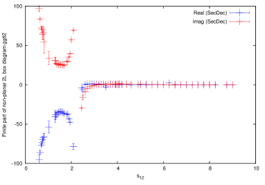
(a) finite part, including threshold

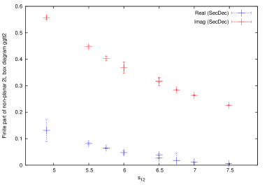
(b) finite part, beyond threshold

Figure 3: Results for the finite part of the scalar integral ggtt2, (a) for a larger kinematic range, (b) zoom into a region further away from threshold. The vertical bars denote the numerical integration errors.

3.1.3 The ggtt1 diagram:

Numerical results for the diagram ggtt1 (see Fig. 2(a)) are shown in Fig. 4 for both the scalar integral and an irreducible rank two tensor integral.

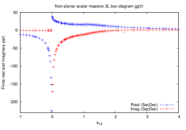
(a) scalar integral

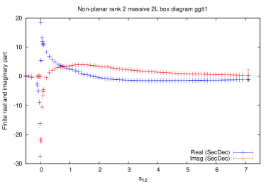
(b) rank 2 tensor integral

Figure 4: Results for the scalar integral ggtt1 shown in Fig. 2(a), and the corresponding rank two tensor integral ggtt1 with $k_{1}\cdot k_{2}$ in the numerator. We vary $s_{12}$ and fix $s_{23}=-1.25,m_{2}=m_{1},p_{3}^{2}=p_{4}^{2}=m_{1}^{2}=1$.

For the results shown in Fig. 4 we used the numerical values $m_{1}^{2}=m_{2}^{2}=m^{2}=1,s_{23}=-1.25,s_{13}=2\,m^{2}-s_{12}-s_{23}$. We set $m_{1}^{2}=m_{2}^{2}$ for the results shown in Fig. 4 because this is the only case occurring in the process $gg\to t\bar{t}$ at two loops if the $b$-quarks are assumed to be massless.

The results shown in Fig. 4(b) correspond to the rank two tensor integral with a factor of $k_{1}\cdot k_{2}$ in the numerator. The numerical integration errors are shown as horizontal markers on the vertical lines. The absence of such markers means that the numerical errors are smaller than visible in the plot.

The timings for one kinematic point for the scalar integral in Fig. 4(a) range from 11-60 secs for points far from threshold to $1.6\times 10^{3}$ seconds for a point very close to threshold, with an average of about 500 secs for points in the vicinity of the threshold. A relative accuracy of $10^{-3}$ has been required for the numerical integration, while the absolute accuracy has been set to $10^{-5}$. For the tensor integral, the timings are better than in the scalar case, as the numerator function present in this case smoothes out the singularity structure. The timings were obtained on a single machine using Intel i7 processors and 8 cores.

3.2 Massive tensor two-loop two-point functions

Here we show that the option to evaluate integrals with a non-trivial numerator can also be applied to calculate two-loop two-point functions involving different mass scales, without the need for a reduction to master integrals. This fact can be used for instance to calculate two-loop corrections to mass parameters in a straightforward way.

As an example we give results for a scalar integral and a rank three tensor integral, where the tensor integral is given by

$$\mathcal{G}_{B} =\left(\frac{1}{\mathrm{i}\pi^{\frac{\mathrm{D}}{2}}}\right)^{2}\int\frac{\mathrm{d^{D}}k_{1}\,\mathrm{d^{D}}k_{2}\,\,(k_{1}\cdot k_{2})\,(k_{1}\cdot p_{1})}{D_{1}\ldots D_{5}}\;\,;\,$$ (12)

$$D_{1}=k_{1}^{2}-m_{1}^{2},D_{2}=(k_{1}+p_{1})^{2}-m_{1}^{2},D_{3}=(k_{1}-k_{2})^{2}-m_{3}^{2},$$

$$D_{4}=(k_{2}+p_{1})^{2}-m_{2}^{2},D_{5}=k_{2}^{2}-m_{2}^{2}\;.$$

The fact that this tensor integral is reducible does not play a role here, because our purpose is to demonstrate that reduction may become obsolete considering the short integration times for the tensors. Results are shown in Fig. 5.

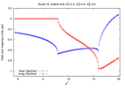
(a) scalar integral

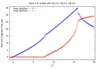
(b) rank 3 tensor integral

Figure 5: Results for the rank 3 two-loop bubble diagram with three non-vanishing masses. (a) scalar case, (b) tensor case with numerator $(k_{1}\cdot k_{2})\,(k_{1}\cdot p_{1})$. The masses are $m_{1}^{2}=2,m_{2}^{2}=4,m_{3}^{2}=3$.

4 Conclusions

We have presented new features of the program SecDec, which can be used to calculate multi-loop integrals numerically in an automated way. Among the new features are the option to directly calculate tensor integrals, and to deal with more general types of integrands than the ones coming directly from standard Feynman integrals. These integrands can be defined by the user, while still profiting from automated processing for the factorisation of the poles and for the numerical integration.

The program is publicly available at http://projects.hepforge.org/secdec.

Acknowledgments

We would like to thank Andreas von Manteuffel for comparisons with analytic results, and the organizers of ACAT2013 for the nice conference.

References

References

- [1] Czakon M and Mitov A 2013 (Preprint 1303.0693)
- [2] Czakon M 2008 Phys.Lett. B664 307–314 (Preprint 0803.1400)
- [3] von Manteuffel A and Studerus C 2013 (Preprint 1306.3504)
- [4] von Manteuffel A and Studerus C Proceedings of the conference “Loops and Legs in Quantum Field Theory”, 2012 (Preprint 1210.1436)
- [5] Bonciani R, Ferroglia A, Gehrmann T, Manteuffel A and Studerus C 2011 JHEP 1101 102 (Preprint 1011.6661)
- [6] Bonciani R, Ferroglia A, Gehrmann T and Studerus C 2009 JHEP 0908 067 (Preprint 0906.3671)
- [7] Bonciani R, Ferroglia A, Gehrmann T, Maitre D and Studerus C 2008 JHEP 0807 129 (Preprint 0806.2301)
- [8] Gehrmann T, Tancredi L and Weihs E 2013 JHEP 1308 070 (Preprint 1306.6344)
- [9] Chachamis G, Czakon M and Eiras D 2008 JHEP 0812 003 (Preprint 0802.4028)
- [10] Carter J and Heinrich G 2011 Comput.Phys.Commun. 182 1566–1581 (Preprint 1011.5493)
- [11] Borowka S, Carter J and Heinrich G 2013 Comput.Phys.Commun. 184 396–408 (Preprint 1204.4152)
- [12] Binoth T and Heinrich G 2000 Nucl. Phys. B585 741–759 (Preprint hep-ph/0004013)
- [13] Roth M and Denner A 1996 Nucl. Phys. B479 495–514 (Preprint hep-ph/9605420)
- [14] Hepp K 1966 Commun. Math. Phys. 2 301–326
- [15] Smirnov A, Smirnov V and Tentyukov M 2011 Comput.Phys.Commun. 182 790–803 (Preprint 0912.0158)
- [16] Bogner C and Weinzierl S 2008 Comput. Phys. Commun. 178 596–610 (Preprint 0709.4092)
- [17] Gluza J, Kajda K, Riemann T and Yundin V 2011 Eur.Phys.J. C71 1516 (Preprint 1010.1667)
- [18] Hahn T 2005 Comput. Phys. Commun. 168 78–95 (Preprint hep-ph/0404043)
- [19] Borowka S and Heinrich G 2013 Comput.Phys.Commun. 184 2552–2561 (Preprint 1303.1157)
- [20] Agrawal S, Hahn T and Mirabella E 2011 (Preprint 1112.0124)
- [21] Heinrich G 2008 Int. J. Mod. Phys. A23 1457–1486 (Preprint 0803.4177)