Scattering of Elastic Waves in a Quasi-one-dimensional Cavity: Theory and Experiment

Abstract

We study the scattering of torsional waves through a quasi-one-dimensional cavity both, from the experimental and theoretical points of view. The experiment consists of an elastic rod with square cross section. In order to form a cavity, a notch at a certain distance of one end of the rod was grooved. To absorb the waves, at the other side of the rod, a wedge, covered by an absorbing foam, was machined. In the theoretical description, the scattering matrix $S$ of the torsional waves was obtained. The distribution of $S$ is given by Poisson’s kernel. The theoretical predictions show an excellent agreement with the experimental results. This experiment corresponds, in quantum mechanics, to the scattering by a delta potential, in one dimension, located at a certain distance from an impenetrable wall.

I Introduction

The scattering of waves by cavities is a problem of interest in several areas of physics. This is due to the fact that cavities present the majority of phenomena observed in the scattering by complex systems MelloKumar ; Beenakker ; Alhassid . The theoretical and numerical studies of scattering by cavities are extensive including the simplest one-dimensional ones MelloKumar ; Gopar ; Martinez-ArguelloMendez-SanchezMartinez-Mares ; Dominguez-RochaMartinez-Mares and the two-dimensional cavities both, integrable and chaotic MelloBaranger ; MelloMartinez-Mares ; Martinez-MaresBaezMendez-Sanchez ; MelloGoparMendez-Bermudez ; Mendez-BermudezLuna-AcostaIzrailev . The quantum graphs KottosSmilansky which also display complex behavior can be considered as one-dimensional scattering cavities.

Up to now, scattering experiments by cavities have been performed using mesoscopic cavities Marcus , quantum corrals Crommie , microwave cavities DoronSmilanskyFrenkel ; LewenkopfMullerDoron ; Mendez-SanchezKuhlBarthLewenkopfStockmann ; SchanzeStockmannMartinez-MaresLewenkopf ; KuhlMartinez-MaresMendez-SanchezStockmann ; Anlage ; Mortessagne2006 ; Richter , optical microcavities NoeckelStone ; Capassoetal and microwave graphs Sirko . In all these experiments the measurements are done in the frequency domain. Wave transport experiments on elastic systems, on the other hand, are scarce and mainly performed in the time domain Fink ; EPL2011 . In this paper we introduce a system in which the transport of elastic waves can be studied in the frequency domain from both, the theoretical and experimental points of view.

We organize the paper as follows. In the next section we propose a theoretical model for the scattering of torsional waves by a one-dimensional cavity in an elastic beam. This is done by grooving of a rectangular notch in a specific place of a semi-infinite beam. The scattering matrix $S$ of this system is obtained and we show that its distribution is correctly described by Poisson’s kernel. In Sec. III we describe the beam used in the experiment: a notch in one side of the beam and a passive vibration isolation system, on the other side. This beam allows the measurement of the scattering of waves by the cavity formed by the notch and the free-end of the beam. In the same section the experimental setup, used to measure the resonances of the elastic cavity, is also presented. In Sec. IV we compare the analytical results with the experiment. Some brief conclusions are given in Sec. V.

II The Theoretical Model and Poisson’s kernel

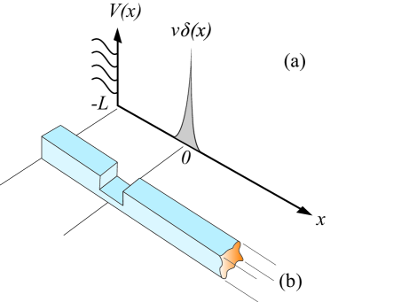
Figure 1: (a) Quantum scattering cavity formed by a delta potential and an impenetrable barrier. (b) An elastic scattering cavity formed by a notch on a semi-infinite rod.

In order to study the resonances of an elastic one-dimensional cavity, lets consider a semi-infinite elastic rod with square cross section of side $W$. As it is shown in Fig. 1, the cavity is formed by a rectangular notch of width $a$ and depth $h$ which have been machined at a distance $L$ from the free-end of the rod. To first order, the torsional wave equation gives a correct description of the scattering of the waves in all regions: inside the cavity, at the notch, and outside the cavity. This model is an analogue of a quantum mechanical delta potential situated at a certain distance from an impenetrable soft wall (Neumann boundary conditions). The solution of the torsional wave equation, in terms of the wave amplitudes in the different regions of the rod (see Fig. 2), can be written as

$$\psi(x)=\left\{\begin{array}[]{ll}A_{1}e^{ikx}+B_{1}e^{-ikx}&\textrm{for }-L\leq x\leq-a/2\\ A_{n}e^{ik_{n}x}+B_{n}e^{-ik_{n}x}&\textrm{for }-a/2\leq x\leq a/2\\ A_{2}e^{-ikx}+B_{2}e^{ikx}&\textrm{for }x\geq a/2\end{array}\right.,$$ (1)

where the wave number $k_{j}$, in the corresponding region of the beam, is given by Graff

$$k_{j}=\frac{2\pi}{c_{j}}f,$$ (2)

with $f$ the frequency and $c_{j}$ the velocity of the waves in the respective region. This velocity is related to the shear modulus $G$ and the density $\rho$, through

$$c_{j}=\sqrt{\frac{G}{\rho}\frac{\alpha_{j}}{I_{j}}},$$ (3)

where $I_{j}$ is the polar momentum of inertia and $\alpha_{j}$ is given by the Navier series in the corresponding region with rectangular cross section whose base is $W_{j}$ and height $h_{j}$ [for $x\in(-L,-a/2)$, $h_{1}=W_{1}=W$, while $h_{n}=W-h$ and $W_{n}=W$ for $x\in(-a/2,a/2)$]; that is,

$$\alpha_{j}=\frac{256}{\pi^{6}}\sum_{m=0}^{\infty}\sum_{p=0}^{\infty}\frac{1}{(2m+1)^{2}(2p+1)^{2}}\frac{h_{j}W_{j}}{(\frac{2m+1}{h_{j}})^{2}+(\frac{2p+1}{W_{j}})^{2}}\,.$$ (4)

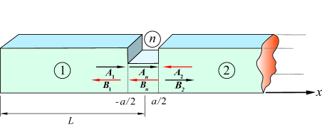
Figure 2: Waves in the different regions of the semi-infinite rod. The width and depth of the notch are $a$ and $h$, respectively. The length of the cavity is $L-a/2$.

Since the one-dimensional cavity has a free-end at $x=-L$, we impose the condition that $d\psi(x)/dx$ vanishes at $x=-L$. We will see below that this boundary condition gives an appropriate description of the experiment. The continuity of $\psi(x)$, as well as of the torsional momentum between the different regions, allows us to obtain the scattering matrix associated to the system, namely

$$S=r_{n}+t_{n}\frac{1}{1-r_{n}e^{2ik(L-a/2)}}e^{2ik(L-a/2)}t_{n},$$ (5)

where $r_{n}$ and $t_{n}$ are the reflection and transmission amplitudes through the notch, given by

$$r_{n}=-\frac{e^{ik_{n}a}-e^{-ik_{n}a}}{\frac{\lambda-1}{\lambda+1}e^{ik_{n}a}-\frac{\lambda+1}{\lambda-1}e^{-ik_{n}a}}$$ (6)

and

$$t_{n}=\frac{\frac{\lambda-1}{\lambda+1}-\frac{\lambda+1}{\lambda-1}}{\frac{\lambda-1}{\lambda+1}e^{ik_{n}a}-\frac{\lambda+1}{\lambda-1}e^{-ik_{n}a}},$$ (7)

where $\lambda=\alpha_{2}/\alpha_{1}$.

Notice that the scattering matrix depends on the frequency through the wave numbers [see Eq. (2)]. With ideal conditions $S(f)$ is an unitary matrix, such that in the $1\times 1$ case it becomes a complex number of unit modulus. In a real situation when $S(f)$ is measured in arbitrary units, as it is the case of elastic systems, its modulus is not unit; that is, $S(f)=\sqrt{R_{0}}\,e^{i\theta(f)}$. Therefore, the movement of $S(f)$ as $f$ is varied, describes a circle of radius $\sqrt{R_{0}}$ in the Argand plane; but it does not visit the circle with the same probability; instead $S(f)$ is distributed according to the non-unitary Poisson’s kernel Martinez-ArguelloMendez-SanchezMartinez-Mares

$$p(\theta)=\frac{1}{2\pi}\frac{R_{0}-\left|\overline{S}\right|^{2}}{\left|S-\overline{S}\right|^{2}},$$ (8)

where $\overline{S}$ is the average of $S(f)$ in frequency which, together with $R_{0}$, is obtained from the experiment. Of course, when $R_{0}=1$, Eq. (8) reduces to the ordinary Poisson’s kernel MelloSeligmanPereyra .

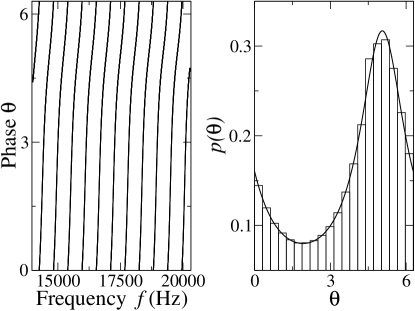
Figure 3: The phase $\theta$ of the $S$-matrix in the frequency range between $14$ kHz and $20$ kHz (left panel). The distribution of $\theta$, for the same numerical data (histogram), agrees with Poisson’s kernel, Eq (8) (continuous line in the right panel).

For the elastic cavity modeled by Eq. (5), $R_{0}=1$ and $\theta$ depends on the frequency but also on the parameters of the rod which are fixed. As an example, we consider a cavity formed on an aluminum rod of square cross section of 25.4 mm of side with a notch of 18.0 mm depth. The physical parameters of the aluminum alloy 6061-T6, that we use in the experiment, are $G=26$ GPa and $\rho=2.7$ g/cm³, such that $\sqrt{G/\rho}=3103.2$ m/s. The numerical resonances of this cavity, eleven in total, are shown in Fig. 3, where $\theta(f)$ is plotted as a function of $f$ for the frequency range between $14$ kHz and $20$ kHz. Also, in Fig. 3 we show the distribution of $\theta$ in this frequency range, which has been obtained numerically and compared with Poisson’s kernel given by Eq. (8) for $R_{0}=1$. The agreement is almost perfect.

III The Experimental Setup

The theoretical model described in the previous section can be studied experimentally in the corresponding elastic system. As it is seen in Fig. 4, we use an aluminum rod with square cross section. This rod is divided in four regions: Region I is the quasi-one-dimensional cavity of length $L-a/2$, where $a$ is the width of a notch of depth $h$, that defines Region II and simulates the quantum delta potential. Regions III and IV mimic the semi-infinite one-dimensional space at the right of the cavity; the vibrations are trapped in a wedge in Region IV which acts as a passive attenuation system, together with a polymeric foam that cover it. This scheme minimizes the reflection at the right-end of the rod and consequently the normal modes of the complete system are diminished; it allows to measure the resonances of the cavity formed by the left free-end of the rod and the notch.

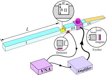
Figure 4: In the system $L=2.5$ m, the depth and width of the notch are $h=0.018$ m and $a=0.0009$ m, respectively. The beam has a total length of $3.6$ m and a square cross-section of $0.0254$ m of side. The wedge has a length of $0.40$ m and it is covered by a polymeric foam. The elastic beam is suspended by two nylon strings (not shown). The connection of the equipment is shown at the bottom.

The elastic system is subject to a torsional elastic excitation via an electromagnetic acoustic transducer (EMAT) disposed in torsional wave configuration MoriFloresGutierrez . The exciter generates a sinusoidal torque at Region III of the elastic system. The excitation of the wave is produced by an oscillating magnetic field of frequency $f$ generated by an AC current $I(t)$ on the EMAT’s coil, at the same frequency. When a paramagnetic metal is close to the EMAT magnetic field, as Faraday’s induction law establishes, eddy currents are produced inside the metal. These currents experience the Lorentz force due to the permanent magnetic field of the EMAT’s magnet. In consequence the metal rotates locally in both directions at the frequency $f$.

The response is detected by a second EMAT located outside the cavity, as shown in Fig. 4. As a detector, the EMAT works in the following way: when a rotating metal is located near the field of a permanent magnet, some loops in the metal will have a non-vanishing variable magnetic flux that will produce eddy currents. These currents will generate an oscillating magnetic field that will be measured by the EMAT’s coil. In this way, the EMAT detector measures the torsional acceleration of diamagnetic metal refEMAT .

To produce the torsional vibration in the elastic system we use a vector network analyzer (VNA, Anritsu MS-4630B). The VNA produces a sinusoidal signal of frequency $f$, which is amplified by a Cerwin-Vega CV-900 amplifier. The amplified signal is sent to the EMAT exciter. The torsional acceleration measured by the EMAT detector is recorded directly by the VNA for its analysis (see Fig. 4).

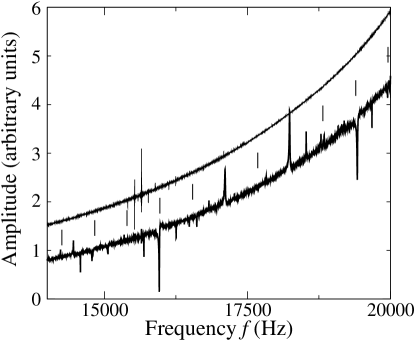
Figure 5: Spectrum measured with the detector located just outside the cavity after the notch (thick line). The thin line corresponds to the base line measured without the magnet of the EMAT detector. The vertical lines correspond to the theoretical predictions obtained from Fig. 3 (see also Table 1 below).

IV Comparison between theory and Experiment

The spectrum of a typical measurement is given in Fig. 5, which shows the observed resonances (thick line). The thin line corresponds to a measurement in which the magnet of the EMAT has been removed; this signal is the impedance curve of the coil and the lines that appear over it are due to radio stations and they must be disregarded. One can observe, also in Fig. 5, that the experimental resonances of the cavity are in very good agreement with the theoretical predictions (vertical marks) of Fig 3. The comparison between the numerical values of the resonances of torsional waves and the predicted ones, is given in Table 1, where errors less than 0.1% are observed. Although some resonances do not appear, they become visible when the location of the EMAT exciter is changed. The remaining resonances belong to other types of vibrations (compressional or flexural).

Resonance	Theory (Hz)	Experiment (Hz)
1	14256	——
2	14826	14819
3	15396	——
4	15966	15960
5	16537	16528
6	17107	17097
7	17677	——
8	18247	18237
9	18818	18800
10	19388	19400
11	19958	19949

Table 1: Torsional resonances of a cavity of length $L=2.5$ m formed by one free end and a notch of width $a=0.0009$ m and depth $h=0.018$ m. The agreement between the theory and experiment is excellent.

Within the frequency range measured, between 14 kHz and 20 kHz, there are eleven resonances. Due to the impedance of the EMAT’s coil, the scattering matrix $S$ describes a circle in the Argand diagram, but displaced from the origin (not shown here). In Fig. 6 we show two of the resonances, (a) 14819 Hz and (b) 15960 Hz (see Table 1), as they are seen from the center of their corresponding circles. In panels (c) and (d) of Fig. 6 we observe the circles whose radii are not the unit. As we previously explain, this is due to the arbitrary units of measurement in the amplitude. In panels (e) and (f) we compare the histograms of their phases with the non-unitary Poisson kernel given by Eq. (8), where the values of the average $\overline{S}$ of the $S$-matrix and their radii, taken as averaged quantities, have been extracted from the corresponding experimental data. As can be seen, the agreement is excellent still for the resonance at $f=14819$ Hz that shows the worst agreement.

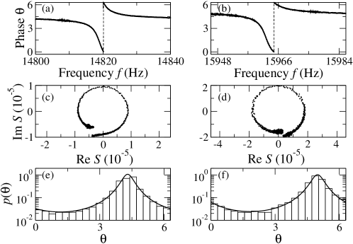
Figure 6: Phase of the $S$-matrix as a function of frequency $f$ (a) for the resonance at 14819 Hz and (b) for the resonance at 15960 Hz. The movement of the $S$-matrix as a function of frequency $f$ in the Argand diagram for the same resonances are given in the panels (c) and (d), respectively. The distributions of the phase in panels (e) and (f) show an excellent agreement with the non-unitary Poisson kernel (continuous line). The resonances are observed from the center of the circles (for explanation see the text).

V Conclusions

We have studied the scattering of torsional waves in a quasi-one-dimensional elastic system. This system consists of a beam with a notch between a free-end and a passive vibration attenuation system that simulates the incoming and outgoing channels at one end of the rod. Theoretically, we obtained the $1\times 1$ scattering matrix from the solution of the torsional wave equation; the numerical predictions helped to select the torsional resonances, among many other vibrational modes that were detected in the experiment. We also verified that the experimental distribution of the phase of the scattering matrix is described by Poisson’s kernel, which is a very important theoretical result in scattering of waves by open systems. Despite that the rod is finite we have confirmed that we opened the system from one side, forming in this way a quasi-one-dimensional open cavity.

VI Acknowledgements

This work was supported by DGAPA-UNAM under project PAPIIT IN111311. MCS and AMMA thank financial support from CONACyT. MMM is grateful with the Sistema Nacional de Investigadores and MA Torres-Segura for her encouragement.

References

- (1) C. W. J. Beenakker, Rev. Mod. Phys. 69, 731 (1997).
- (2) Y. Alhassid, Rev. Mod. Phys. 72, 895 (2000).
- (3) P. A. Mello and N. Kumar, Quantum Transport in Mesoscopic Systems: Complexity and Statistical Fluctuations (Oxford University Press, New York, 2005).
- (4) V. A. Gopar, Electronic transport in mesoscopic systems. An approach based on random matrices at one and various energies, Ph. D. thesis (Universidad Nacional Autónoma de México, Distrito Federal, 1999).
- (5) A. M. Martínez-Argüello, R. A. Méndez-Sánchez, and M. Martínez-Mares, Phys. Rev. E. 86, 016207 (2012).
- (6) V. Domínguez-Rocha and M. Martínez-Mares, J. Phys. A: Math. Theor. 46, 235101 (2013).
- (7) P. A. Mello, H. Baranger, Interference phenomena in electronic transport through chaotic cavities: An information-theoretic approach, AIP Conf. Proc. No. 464 (AIP, Melville, NY, 2008).
- (8) G. Báez, M. Martínez-Mares, and R. A. Méndez-Sánchez, Phys. Rev. E. 78, 036208 (2008).
- (9) J. A. Méndez-Bermúdez, G. A. Luna-Acosta, and F. M. Izrailev, Physica E 22, 881 (2004).
- (10) P. A. Mello and M. Martínez-Mares, Phys. Rev. E. 63, 016205 (2000).
- (11) P. A. Mello, V. A. Gopar, and J. A. Méndez-Bermúdez, Comments: Conference Proceedings: Chaos 2009, Chania, Crete, Greece.
- (12) T. Kottos and U. Smilansky, Phys. Rev. Lett. 79, 4794 (1997).
- (13) C. M. Marcus, A. J. Rimberg, R. M. Westervelt, P. F. Hopkins, and A. C. Gossard, Phys. Rev. Lett. 69, 506 (1992).
- (14) M. F. Crommie, C. P. Lutz, and D. M. Eigler, Nature 363, 524 (1993).
- (15) E. Doron, U. Smilansky, and A. Frenkel, Phys. Rev. Lett. 65, 3072 (1990).
- (16) C. H. Lewenkopf, A. Müller, and E. Doron, Phys. Rev. A 45, 2635 (1992).
- (17) R. A. Méndez-Sánchez, U. Kuhl, M. Barth, C. H. Lewenkopf, and H.-J. Stöckmann, Phys. Rev. Lett. 91, 174102 (2003).
- (18) H. Schanze, H. J. Stöckmann, M. Martínez-Mares, and C. H. Lewenkopf Phys. Rev. E 71, 016223 (2005).
- (19) U. Kuhl, M. Martínez-Mares, R. A. Méndez-Sánchez, and H.-J. Stöckmann, Phys. Rev. Lett. 94, 144101 (2005).
- (20) S. Hemmady, X. Zheng, E. Ott, T. M. Antonsen, Jr., and S. M. Anlage, Phys. Rev. Lett. 94, 014102 (2005).
- (21) D. Laurent, O. Legrand, and F. Mortessagne, Phys. Rev. E. 74, 046219 (2006).
- (22) S. Bittner, B. Dietz, M. Miski-Oglu, P. O. Iriarte, A. Richter, and F. Schäfer, Phys. Rev. E. 84, 016221 (2011).
- (23) J. U. Nöckel and A. D. Stone, Nature 385, 45 (1997).
- (24) P. Malara, R. Blanchard, T. S. Mansuripur, A. K. Wojcik, A. Belyanin, K. Fujita, T. Edamura, S. Furuta, M. Yamanishi, P. de Natale, and F. Capasso, Appl. Phys. Lett. 102, 141105 (2013).
- (25) O. Hul, O. Tymoshchuk, S. Bauch, P. M. Koch, and L. Sirko, J. Phys. A: Math. Gen. 38, 10489 (2005).
- (26) S. Catheline, N. Benech, J. Brum, and C. Negreira, Phys. Rev. Lett. 100, 064301 (2008).
- (27) A. Morales, A. Díaz-de-Anda, J. Flores, L. Gutiérrez, R. A. Méndez-Sánchez, G. Monsivais, and P. Mora, Europhys. Lett. 99, 54002 (2012).
- (28) K. F. Graff, Wave motion in Elastic Solids (Dover, New York, 1991).
- (29) P. A. Mello, P. Pereyra, and T. H. Seligman, Ann. Phys. (NY) 161, 254 (1985).
- (30) A. Morales, J. Flores, L. Gutiérrez, and R. A. Méndez-Sánchez, J. Acoust. Soc. Am. 112, 1961 (2002).
- (31) A. Morales, L. Gutiérrez, and J. Flores, Am. J. Phys. 69, 519 (2001).