A Model for Soft High-Energy Scattering:
Tensor Pomeron and Vector Odderon

Carlo Ewerz ^a,b,1, Markos Maniatis ^c,2,
Otto Nachtmann ^a,3

^a Institut für Theoretische Physik, Universität Heidelberg
Philosophenweg 16, D-69120 Heidelberg, Germany

^b ExtreMe Matter Institute EMMI, GSI Helmholtzzentrum für Schwerionenforschung
Planckstraße 1, D-64291 Darmstadt, Germany

^c Departamento de Ciencias Básicas, Universidad del Bío-Bío
Avda. Andrés Bello s/n, Casilla 447, Chillán 3780000, Chile

A model for soft high-energy scattering is developed. The model is formulated in terms of effective propagators and vertices for the exchange objects: the pomeron, the odderon, and the reggeons. The vertices are required to respect standard rules of QFT. The propagators are constructed taking into account the crossing properties of amplitudes in QFT and the power-law ansätze from the Regge model. We propose to describe the pomeron as an effective spin 2 exchange. This tensor pomeron gives, at high energies, the same results for the $pp$ and $p\bar{p}$ elastic amplitudes as the standard Donnachie-Landshoff pomeron. But with our tensor pomeron it is much more natural to write down effective vertices of all kinds which respect the rules of QFT. This is particularly clear for the coupling of the pomeron to particles carrying spin, for instance vector mesons. We describe the odderon as an effective vector exchange. We emphasise that with a tensor pomeron and a vector odderon the corresponding charge-conjugation relations are automatically fulfilled. We compare the model to some experimental data, in particular to data for the total cross sections, in order to determine the model parameters. The model should provide a starting point for a general framework for describing soft high-energy reactions. It should give to experimentalists an easily manageable tool for calculating amplitudes for such reactions and for obtaining predictions which can be compared in detail with data.

  ¹ email: C.Ewerz@thphys.uni-heidelberg.de
² email: mmaniatis@ubiobio.cl
³ email: O.Nachtmann@thphys.uni-heidelberg.de

1 Introduction

Today we have a well-established theory of strong interactions, quantum chromodynamics (QCD). Thus, in principle, all strong-interaction phenomena should be describable in terms of the fundamental QCD Lagrangian. In practice, this goal is in essence achieved for short distance phenomena due to asymptotic freedom [1, 2]. Pure long-distance phenomena can be treated by lattice methods introduced for QCD in [3]. But soft high-energy scattering where the c. m. energy $\sqrt{s}$ of the collision becomes large but the momentum transfer $\sqrt{|t|}$ stays small is neither a pure short distance nor a pure long distance phenomenon. Thus, when an experimentalist asks a theorist to calculate the cross section for a given soft high-energy reaction the theorist will have to resort to models. And indeed, there is a time-honoured model, the Regge model, which describes many observed regularities of soft high-energy scattering; see for instance [4, 5, 6, 7, 8, 9, 10, 11]. Now we were indeed interested in calculating the amplitude for a specific process: photoproduction of a $\pi^{+}\pi^{-}$ pair on a proton

$$\gamma+p\longrightarrow\pi^{+}+\pi^{-}+p\,.$$ (1.1)

For this calculation we wanted to include not only pomeron but also reggeon, photon, and odderon exchange. We were then confronted with a problem. Simple and handy rules for calculations of soft high-energy reactions were hard to find. We thought that such rules should be formulated in terms of effective propagators and vertices. For a given process these propagators and vertices should then be combinable according to the standard rules of quantum field theory (QFT). In the present paper we shall formulate such rules. We shall also present a formulation of the exchanges of the pomeron and the odderon as effective spin 2 and spin 1 exchanges, respectively. Let us recall that the pomeron has charge conjugation $C=+1$ and is ubiquitous in high-energy reactions. On the other hand, the odderon with $C=-1$, introduced theoretically in [12, 13], is still elusive in experiments; see [14] for a review. As we shall see, considering the pomeron as an effective spin 2 exchange presents advantages compared to viewing it as the exchange of an effective $C=+1$ ‘photon’ [15, 16, 17, 18]. With an effective spin 2 pomeron it is easy to respect all rules of QFT. Moreover, it turns out that in this framework applications of the vector meson-dominance (VMD) model to photon-induced reactions are straightforward and do not lead to gauge-invariance problems.

Our paper is organised as follows. In section 2 we list the reactions which we want to consider and identify the exchanges and vertices needed for calculating the corresponding amplitudes. In section 3 the rules for these exchanges and vertices are given. In sections 4 to 7 we explain how we arrive at these rules. Section 8 contains our conclusions. In a companion paper [19] we will treat in detail reaction (1.1) which is suitable for an odderon search.

2 The Reactions

In this section we list the reactions to be studied in the framework of our model. These are high-energy reactions and decay processes. The former will be described in terms of Regge exchanges, and we use the conventional names for the Regge trajectories: ${\mathbbm{P}}$ (pomeron), ${\mathbbm{O}}$ (odderon), $\rho_{R}$ ($\rho$ reggeon), $\omega_{R}$ ($\omega$ reggeon), $f_{2R}$ ($f_{2}$ reggeon), $a_{2R}$ ($a_{2}$ reggeon). The expressions which we use for the effective propagators and vertices of these objects are presented in section 3 below. In table 1 we list the quantum numbers $C$ of charge conjugation and $G$ of $G$ parity for those particles and exchange objects which are eigenstates of $C$ respectively $G$. We recall that the $G$ parity operator is defined as

$$G=\exp(i\pi I_{2})\,C$$ (2.1)

where $I_{2}$ is the second component of the isospin operator. $C$ invariance holds for strong and electromagnetic interactions, whereas $G$ invariance only holds for strong interactions. Here and in the following the particles $f_{2}$ and $a_{2}$ are understood as $f_{2}(1270)$ and the neutral $a_{2}(1320)$, respectively, in the PDG list [20].

particles	$C$	$G$
$\pi^{0}$	$1$	$-1$
$\pi^{\pm}$		$-1$
$\rho^{0}$	$-1$	$1$
$\rho^{\pm}$		$1$
$\omega$	$-1$	$-1$
$f_{2}$	$1$	$1$
$a_{2}$	$1$	$-1$

exchanges	$C$	$G$
${\mathbbm{P}}$	$1$	$1$
${\mathbbm{O}}$	$-1$	$-1$
$\rho_{R}$	$-1$	$1$
$\omega_{R}$	$-1$	$-1$
$f_{2R}$	$1$	$1$
$a_{2R}$	$1$	$-1$

Table 1: The charge conjugation and $G$-parity quantum numbers of particles and exchange objects.

For high energy reactions we use the Mandelstam variables, $s$ the c. m. energy squared, and $t$ the momentum transfer squared.

• Soft high energy reactions to be considered:

  $$p+p\longrightarrow p+p\,,$$ (2.2)

  $$p+\bar{p}\longrightarrow p+\bar{p}\,,$$ (2.3)

  $$p+n\longrightarrow p+n\,,$$ (2.4)

  $$\bar{p}+n\longrightarrow\bar{p}+n\,,$$ (2.5)

  $$\pi+p\longrightarrow\pi+p\,,$$ (2.6)

  $$\rho+p\longrightarrow\rho+p\,.$$ (2.7)

  The diagrams for (2.2) are shown in figure 1. The diagrams for (2.3) to (2.5) are analogous. The diagrams for (2.6) are shown in figure 2. Of course, single $\gamma$ exchange only contributes to $\pi^{\pm}p\to\pi^{\pm}p$ and is absent for $\pi^{0}p\to\pi^{0}p$. Note that $G$ parity invariance forbids the vertices $a_{2R}\pi\pi$, $\omega_{R}\pi\pi$ and ${\mathbbm{O}}\pi\pi$; see table 1. Thus, the exchanges of $a_{2R},\omega_{R}$, and ${\mathbbm{O}}$ cannot contribute to the reaction (2.6). For $\rho p$ scattering (2.7) the diagrams are shown in figure 3 where $\rho_{R}$ and $\gamma$ exchange only contribute to $\rho^{\pm}p\to\rho^{\pm}p$. This brings us to the decay reactions which we want to consider.

  

  

  

  

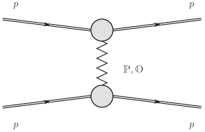
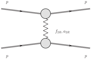
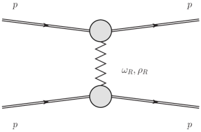
  Figure 1: Diagrams for $pp\to pp$ (2.2) at high energies.

  

  

  

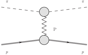
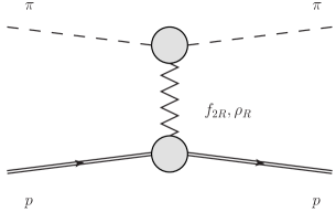
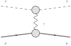
  Figure 2: Diagrams for $\pi p\to\pi p$ (2.6) at high energies.

  

  

  

  

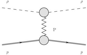
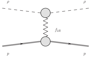
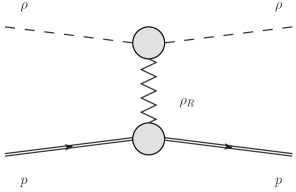
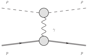
  Figure 3: Diagrams for $\rho p\to\rho p$ (2.7) at high energies.

• Decay reactions to be considered:

  $$\rho^{0} \longrightarrow\pi^{+}+\pi^{-}\,,$$ (2.8)

  $$f_{2} \longrightarrow\pi^{+}+\pi^{-}\,,\,\pi^{0}+\pi^{0}\,,$$ (2.9)

  $$f_{2} \longrightarrow\gamma+\gamma\,,$$ (2.10)

  $$a_{2} \longrightarrow\gamma+\gamma\,.$$ (2.11)

In the following we will discuss the propagators and vertices needed for calculating the diagrams corresponding to the scattering reactions (2.2) to (2.7) and to the decay reactions (2.8) to (2.11). We shall encounter vertices with reggeons and particles, for instance the $f_{2R}\pi\pi$ and the $f_{2}\pi\pi$ vertices. We formulate here the hypothesis that the coupling constants of corresponding reggeon-particle and particle-particle vertices are approximately equal. We will find support for this hypothesis in various cases from data. In other cases we shall use the hypothesis just to get estimates for coupling constants.

The methods which we shall develop in the following for describing the reactions (2.2) to (2.11) can easily be extended to the treatment of various other processes. For example, the inclusion of strange particles and corresponding trajectories would be straightforward. We leave this for future work.

3 Propagators and Vertices

In this section we give the analytic expressions for the propagators and vertices needed for calculating the amplitudes for the reactions listed in section 2. We also give standard or default values for the parameters occurring. The justifications for these expressions and parameters will be given in later sections. The conventions for kinematics and Dirac $\gamma$ matrices follow [21].

At this point it is appropriate to say something about the errors of the parameters listed in the following. Whenever errors are available, for instance for numbers taken from [20], these are quoted. Some numbers which we take from [9] are given there without errors. We estimate these errors to be at the 5 to 10% level in general. In some cases numbers which we derive have even larger errors, maybe up to 30%. Of course, we would like to know all parameters of our model as accurately as possible. The hope is that in the future, using our framework, one will be able to make global fits to data on soft reactions and determine the corresponding parameters together with realistic uncertainties.

3.1 Propagators and Effective Propagators

$\bullet$ photon $\gamma$
     

$$i\Delta_{\mu\nu}^{(\gamma)}(k)=\frac{-ig_{\mu\nu}}{k^{2}+i\epsilon}\,.$$ (3.1)

$\bullet$ vector mesons $V=\rho^{0},\omega$ (see section 4)
     

$$i\Delta_{\mu\nu}^{(V)}(k)=i\left(-g_{\mu\nu}+\frac{k_{\mu}k_{\nu}}{k^{2}+i\epsilon}\right)\Delta_{T}^{(V)}(k^{2})-i\frac{k_{\mu}k_{\nu}}{k^{2}+i\epsilon}\Delta_{L}^{(V)}(k^{2})\,.$$ (3.2)

Here $\Delta_{T}^{(V)}(k^{2})$ and $\Delta_{L}^{(V)}(k^{2})$ are the invariant functions in the transverse and longitudinal parts, respectively, of the propagators.

For a careful discussion of the propagator matrix of the $\gamma$-$\rho$-$\omega$ system we refer to [22]. In Appendix B of [22] analytic formulae for the $\gamma$-$\rho$-$\omega$ propagator matrix are given. With the normalisation used there we get

$$\begin{split}\Delta_{T}^{(\rho)}(0)=-1/m_{\rho}^{2}\,,\\ \Delta_{T}^{(\omega)}(0)=-1/m_{\omega}^{2}\,.\end{split}$$ (3.3)

The longitudinal functions $\Delta_{L}^{(V)}(k^{2})$ need not be specified since they will never enter our calculations. The transverse functions $\Delta_{T}^{(V)}(k^{2})$ will be discussed in detail in section 4. We quote here the values for the masses $m_{V}$ and the widths $\Gamma_{V}$ ($V=\rho^{0},\omega$) from [20]:

$$\begin{split}m_{\rho^{0}}&=775.49\pm 0.34\,\mbox{MeV}\,,\>\>\>\>\>\>\Gamma_{\rho^{0}}=146.2\pm 0.7\,\mbox{MeV}\,,\\ m_{\omega}&=782.65\pm 0.12\,\mbox{MeV}\,,\>\>\>\>\>\>\Gamma_{\omega}=8.49\pm 0.08\,\mbox{MeV}\,.\end{split}$$ (3.4)

We note that only for qualitative calculations not aiming at too high accuracy and neglecting $\rho$-$\omega$ interference one may use, for $k^{2}$ away from zero, the simple Breit-Wigner expressions for $\Delta^{(V)}_{T}(k^{2})$,

$$\Delta_{T}^{(V)}(k^{2})=\frac{1}{k^{2}-m_{V}^{2}+im_{V}\Gamma_{V}}\,.$$ (3.5)

$\bullet$ tensor meson $f_{2}\equiv f_{2}(1270)$ (see section 5)
     

$$\begin{split}i\Delta^{(f_{2})}_{\mu\nu,\kappa\lambda}(k)=\,i\,\bigg{\{}&\frac{1}{2}\left(-g_{\mu\kappa}+\frac{k_{\mu}k_{\kappa}}{k^{2}+i\epsilon}\right)\left(-g_{\nu\lambda}+\frac{k_{\nu}k_{\lambda}}{k^{2}+i\epsilon}\right)\\ &+\frac{1}{2}\left(-g_{\mu\lambda}+\frac{k_{\mu}k_{\lambda}}{k^{2}+i\epsilon}\right)\left(-g_{\nu\kappa}+\frac{k_{\nu}k_{\kappa}}{k^{2}+i\epsilon}\right)\\ &-\frac{1}{3}\left(-g_{\mu\nu}+\frac{k_{\mu}k_{\nu}}{k^{2}+i\epsilon}\right)\left(-g_{\kappa\lambda}+\frac{k_{\kappa}k_{\lambda}}{k^{2}+i\epsilon}\right)\bigg{\}}\,\Delta^{(2)}(k^{2})\,.\end{split}$$ (3.6)

Here we only give the spin 2 part of the corresponding tensor-field propagator. The invariant function $\Delta^{(2)}(k^{2})$ is the one where the $f_{2}$ meson appears; see (5.22) in section 5. We have the following relations:

$$\Delta^{(f_{2})}_{\mu\nu,\kappa\lambda}(k)=\Delta^{(f_{2})}_{\nu\mu,\kappa\lambda}(k)=\Delta^{(f_{2})}_{\mu\nu,\lambda\kappa}(k)=\Delta^{(f_{2})}_{\kappa\lambda,\mu\nu}(k)\,,$$ (3.7)

$$\begin{split}g^{\mu\nu}\Delta^{(f_{2})}_{\mu\nu,\kappa\lambda}(k)&=0\,,\\ g^{\kappa\lambda}\Delta^{(f_{2})}_{\mu\nu,\kappa\lambda}(k)&=0\,.\end{split}$$ (3.8)

From [20] we have for the mass and width of the $f_{2}$ meson

$$m_{f_{2}}=1275.1\pm 1.2\,\mbox{MeV}\,,\>\>\>\>\>\>\Gamma_{f_{2}}=185.1\,{}^{+2.9}_{-2.4}\,\mbox{MeV}\,.$$ (3.9)

$\bullet$ pomeron ${\mathbbm{P}}$ (see section 6.1)
     

$$i\Delta^{(\mathbbm{P})}_{\mu\nu,\kappa\lambda}(s,t)=\frac{1}{4s}\left(g_{\mu\kappa}g_{\nu\lambda}+g_{\mu\lambda}g_{\nu\kappa}-\frac{1}{2}g_{\mu\nu}g_{\kappa\lambda}\right)\,(-is\alpha^{\prime}_{\mathbbm{P}})^{\alpha_{\mathbbm{P}}(t)-1}\,,$$ (3.10)

$$\begin{split}\alpha_{\mathbbm{P}}(t)&=1+\epsilon_{\mathbbm{P}}+\alpha^{\prime}_{\mathbbm{P}}t\,,\\ \epsilon_{\mathbbm{P}}&=0.0808\,,\\ \alpha^{\prime}_{\mathbbm{P}}&=0.25\,\mbox{GeV}^{-2}\,.\end{split}$$ (3.11)

$\bullet$ reggeons ${\mathbbm{R}}_{+}=f_{2R},a_{2R}$ (see section 6.3)
     

$$i\Delta^{(\mathbbm{R}_{+})}_{\mu\nu,\kappa\lambda}(s,t)=\frac{1}{4s}\left(g_{\mu\kappa}g_{\nu\lambda}+g_{\mu\lambda}g_{\nu\kappa}-\frac{1}{2}g_{\mu\nu}g_{\kappa\lambda}\right)(-is\alpha^{\prime}_{\mathbbm{R}_{+}})^{\alpha_{\mathbbm{R}_{+}}(t)-1}\,,$$ (3.12)

$$\begin{split}\alpha_{\mathbbm{R}_{+}}(t)&=\alpha_{\mathbbm{R}_{+}}(0)+\alpha^{\prime}_{\mathbbm{R}_{+}}t\,,\\ \alpha_{\mathbbm{R}_{+}}(0)&=0.5475\,,\\ \alpha^{\prime}_{\mathbbm{R}_{+}}&=0.9\,\mbox{GeV}^{-2}\,.\end{split}$$ (3.13)

$\bullet$ reggeons ${\mathbbm{R}}_{-}=\omega_{R},\rho_{R}$ (see section 6.3)
     

$$i\Delta_{\mu\nu}^{(\mathbbm{R}_{-})}(s,t)=ig_{\mu\nu}\,\frac{1}{M_{-}^{2}}\,(-is\alpha^{\prime}_{\mathbbm{R}_{-}})^{\alpha_{\mathbbm{R}_{-}}(t)-1}\,,$$ (3.14)

$$\begin{split}\alpha_{\mathbbm{R}_{-}}(t)&=\alpha_{\mathbbm{R}_{-}}(0)+\alpha^{\prime}_{\mathbbm{R}_{-}}t\,,\\ \alpha_{\mathbbm{R}_{-}}(0)&=0.5475\,,\\ \alpha^{\prime}_{\mathbbm{R}_{-}}&=0.9\,\mbox{GeV}^{-2}\,,\\ M_{-}&=1.41\,\mbox{GeV}\,.\end{split}$$ (3.15)

The numbers for the parameters in (3.11), (3.13) and (3.15) are taken from [9], except for $M_{-}$ which is discussed in section 6.3.

$\bullet$ odderon ${\mathbbm{O}}$ (see section 6.2)
     

$$i\Delta_{\mu\nu}^{(\mathbbm{O})}(s,t)=-ig_{\mu\nu}\,\frac{\eta_{\mathbbm{O}}}{M_{0}^{2}}\,(-is\alpha^{\prime}_{\mathbbm{O}})^{\alpha_{\mathbbm{O}}(t)-1}\,,$$ (3.16)

$$\begin{split}\alpha_{\mathbbm{O}}(t)&=1+\epsilon_{\mathbbm{O}}+\alpha^{\prime}_{\mathbbm{O}}t\,,\\ M_{0}&=1\,\mbox{GeV}\,,\\ \eta_{\mathbbm{O}}&=\pm 1\,,\\ \alpha^{\prime}_{\mathbbm{O}}&=0.25\,\mbox{GeV}^{-2}\,.\end{split}$$ (3.17)

The odderon parameters $\epsilon_{\mathbbm{O}}$, $\alpha^{\prime}_{\mathbbm{O}}$, and $\eta_{\mathbbm{O}}$ are at present not known experimentally. In (3.16) we have put $M_{0}^{-2}$ for dimensional reasons. We note that another overall scale factor in the propagator instead of $M_{0}^{-2}$ can always be traded against scale factors in the odderon vertices; see section 6.2. We have, furthermore, assumed $\alpha^{\prime}_{\mathbbm{O}}=\alpha^{\prime}_{\mathbbm{P}}$ in (3.17) for lack of other information.

3.2 Vertices and Effective Vertices

In this section we list the vertices and effective vertices which we need for the discussion of the reactions of section 2. For writing down these vertices we shall frequently use two rank-four tensor functions defined as follows

$$\Gamma_{\mu\nu\kappa\lambda}^{(0)}(k_{1},k_{2})=\, [(k_{1}\cdot k_{2})g_{\mu\nu}-k_{2\mu}k_{1\nu}]\left[k_{1\kappa}k_{2\lambda}+k_{2\kappa}k_{1\lambda}-\frac{1}{2}(k_{1}\cdot k_{2})g_{\kappa\lambda}\right]\,,$$ (3.18)

$$\Gamma_{\mu\nu\kappa\lambda}^{(2)}(k_{1},k_{2})=\, (k_{1}\cdot k_{2})(g_{\mu\kappa}g_{\nu\lambda}+g_{\mu\lambda}g_{\nu\kappa})+g_{\mu\nu}(k_{1\kappa}k_{2\lambda}+k_{2\kappa}k_{1\lambda})$$

$$-k_{1\nu}k_{2\lambda}g_{\mu\kappa}-k_{1\nu}k_{2\kappa}g_{\mu\lambda}-k_{2\mu}k_{1\lambda}g_{\nu\kappa}-k_{2\mu}k_{1\kappa}g_{\nu\lambda}$$ (3.19)

$$-[(k_{1}\cdot k_{2})g_{\mu\nu}-k_{2\mu}k_{1\nu}]\,g_{\kappa\lambda}\,.$$

We have for $i=0,2$

$$\Gamma_{\mu\nu\kappa\lambda}^{(i)}(k_{1},k_{2})=\Gamma_{\mu\nu\lambda\kappa}^{(i)}(k_{1},k_{2})=\Gamma_{\nu\mu\kappa\lambda}^{(i)}(k_{2},k_{1})=\Gamma_{\mu\nu\kappa\lambda}^{(i)}(-k_{1},-k_{2})\,,$$ (3.20)

$$\begin{split}&k_{1}^{\mu}\Gamma_{\mu\nu\kappa\lambda}^{(i)}(k_{1},k_{2})=0\,,\\ &k_{2}^{\nu}\Gamma_{\mu\nu\kappa\lambda}^{(i)}(k_{1},k_{2})=0\,,\end{split}$$ (3.21)

$$\Gamma_{\mu\nu\kappa\lambda}^{(i)}(k_{1},k_{2})\,g^{\kappa\lambda}=0\,.$$ (3.22)

Now here is our list of vertices.

$\bullet$ $\gamma V$, where $V=\rho,\omega,\phi$ (see eq. (5.3) of [9] and section 4)
     

$$-ie\,\frac{m_{V}^{2}}{\gamma_{V}}\,g_{\mu\nu}\,,$$ (3.23)

$$e>0\,,\quad\gamma_{\rho}>0\,,\quad\gamma_{\omega}>0\,,\quad\gamma_{\phi}<0\,,$$ (3.24)

$$\frac{4\pi}{\gamma_{\rho}^{2}}=0.496\pm 0.023\,,\quad\frac{4\pi}{\gamma_{\omega}^{2}}=0.042\pm 0.0015\,,\quad\frac{4\pi}{\gamma_{\phi}^{2}}=0.0716\pm 0.0017\,.$$ (3.25)

$\bullet$ $\gamma pp$
     

$$i\Gamma_{\mu}^{(\gamma pp)}(p^{\prime},p)=-ie\left[\gamma_{\mu}F_{1}(t)+\frac{i}{2m_{p}}\,\sigma_{\mu\nu}(p^{\prime}-p)^{\nu}F_{2}(t)\right]\,,$$ (3.26)

$$e>0\,,\qquad t=(p^{\prime}-p)^{2}\,,$$ (3.27)

$$\sigma_{\mu\nu}=\frac{i}{2}\left(\gamma_{\mu}\gamma_{\nu}-\gamma_{\nu}\gamma_{\mu}\right)\,,$$ (3.28)

$$F_{1}(t) =\left(1-\frac{t}{4m_{p}^{2}}\frac{\mu_{p}}{\mu_{N}}\right)\left(1-\frac{t}{4m_{p}^{2}}\right)^{-1}G_{D}(t)\,,$$ (3.29)

$$F_{2}(t) =\left(\frac{\mu_{p}}{\mu_{N}}-1\right)\left(1-\frac{t}{4m_{p}^{2}}\right)^{-1}G_{D}(t)\,,$$ (3.30)

$$\mu_{N}=\frac{e}{2m_{p}}\,,\qquad\frac{\mu_{p}}{\mu_{N}}=2.7928\,,$$ (3.31)

$$G_{D}(t)=\left(1-\frac{t}{m_{D}^{2}}\right)^{-2}\,,\qquad m_{D}^{2}=0.71\,\mbox{GeV}^{2}\,.$$ (3.32)

The $\gamma pp$ vertex is, of course, well known and we use here standard parametrisations for $F_{1,2}(t)$; see for instance chapter 2 in [23]. $F_{1}$ and $F_{2}$ are the Dirac and Pauli form factors of the proton, respectively, and $G_{D}$ is the so-called dipole form factor.

$\bullet$ $\gamma nn$
     

$$i\Gamma_{\mu}^{(\gamma nn)}(p^{\prime},p)=-ie\left[\gamma_{\mu}F^{n}_{1}(t)+\frac{i}{2m_{n}}\sigma_{\mu\nu}(p^{\prime}-p)^{\nu}F^{n}_{2}(t)\right]\,.$$ (3.33)

The neutron form factors $F^{n}_{1,2}(t)$ are less well known than those of the proton. We have $F^{n}_{1}(0)=0$ as the neutron is electrically neutral. In the reactions that we want to consider the $\gamma nn$ vertex is not relevant and we will not discuss it further here.

In the hadronic vertices listed in the following we have to take into account form factors since the hadrons are extended objects. For simplicity we use for the pomeron-nucleon coupling the electromagnetic Dirac form factor $F_{1}(t)$ of the proton (3.29), as suggested in [16]; see also chapter 3.2 of [9]. The same ansatz is made for the reggeon-nucleon and the odderon-nucleon couplings. In the corresponding couplings of pomeron, odderon and reggeons to mesons we always use the pion electromagnetic form factor in a simple parametrisation

$$F_{M}(t)=F_{\pi}(t)=\frac{m_{0}^{2}}{m_{0}^{2}-t}\,,$$ (3.34)

with $m_{0}^{2}=0.50$ GeV²; see eq. (3.22) in chapter 3.2 of [9] where it is also discussed why these assumptions cannot be true in general but should be a reasonable approximation for $0\leq-t\leq 1$ GeV². Note that we do not use for $F_{\pi}(t)$ in (3.34) the canonical vector-meson-dominance (VMD) form which would correspond to replacing $m^{2}_{0}$ by $m^{2}_{\rho}\approx 0.60$ GeV². Indeed, for $t<0$ the measured pion form factor squared is smaller than given by the canonical VMD form (see for instance figure 4 of [22]) and this is taken into account by having $m^{2}_{0}<m^{2}_{\rho}$ in (3.34).

$\bullet$ $\rho^{0}\pi^{+}\pi^{-}$ (see section 4, eq. (4.25))
     

$$i\Gamma_{\mu}^{(\rho\pi\pi)}(k_{1},k_{2})=-\frac{1}{2}ig_{\rho\pi\pi}(k_{1}-k_{2})_{\mu}\,,$$ (3.35)

$$g_{\rho\pi\pi}=11.51\pm 0.07\,.$$ (3.36)

$\bullet$ $f_{2}\pi\pi$ (see section 5.1)
           
In the limit of strict isospin invariance both diagrams are described by the same expression

$$i\Gamma_{\kappa\lambda}^{(f_{2}\pi\pi)}(k_{1},k_{2})=-i\,\frac{g_{f_{2}\pi\pi}}{2M_{0}}\left[(k_{1}-k_{2})_{\kappa}(k_{1}-k_{2})_{\lambda}-\frac{1}{4}g_{\kappa\lambda}(k_{1}-k_{2})^{2}\right]F^{(f_{2}\pi\pi)}(k^{2})\,,$$ (3.37)

with $k=k_{1}+k_{2}$ and

$$g_{f_{2}\pi\pi}=9.26\pm 0.15\,,\qquad M_{0}=1\,\mbox{GeV}\,.$$ (3.38)

Here $F^{(f_{2}\pi\pi)}(k^{2})$ is a form factor normalised to $F^{(f_{2}\pi\pi)}(m_{f_{2}}^{2})=1$; see section 5.1.

For production processes of $f_{2}$ decaying then to $\pi^{+}\pi^{-}$, for example, we are also interested in the $\pi\pi$ invariant mass distribution. Thus, the couplings like $f_{2}\pi\pi$ are not only needed for the ”on-shell” $f_{2}$ but also away from the mass shell, for $k^{2}\neq m_{f_{2}}^{2}$. Realistically, as done in (3.37), we have to introduce form factors to describe the $k^{2}$ dependence of these couplings. These form factors will be normalised to $1$ at the on-shell point.

$\bullet$ $f_{2}\gamma\gamma$ (see sections 5.3 and 7.2)
     

$$\begin{split}i\Gamma_{\mu\nu\kappa\lambda}^{(f_{2}\gamma\gamma)}(k_{1},k_{2})=\,&iF_{M}(k_{1}^{2})F_{M}(k_{2}^{2})F^{(f_{2}\gamma\gamma)}(k^{2})\\ &\times\left[2a_{f_{2}\gamma\gamma}\Gamma_{\mu\nu\kappa\lambda}^{(0)}(k_{1},k_{2})-b_{f_{2}\gamma\gamma}\Gamma_{\mu\nu\kappa\lambda}^{(2)}(k_{1},k_{2})\right]\,,\end{split}$$ (3.39)

with $k=k_{1}+k_{2}$ and

$$a_{f_{2}\gamma\gamma}=\frac{e^{2}}{4\pi}\,1.45\,\mbox{GeV}^{-3}\,,\qquad b_{f_{2}\gamma\gamma}=\frac{e^{2}}{4\pi}\,2.49\,\mbox{GeV}^{-1}\,.$$ (3.40)

Here $F^{(f_{2}\gamma\gamma)}(k^{2})$ is a form factor normalised to $F^{(f_{2}\gamma\gamma)}(m_{f_{2}}^{2})=1$.

$\bullet$ $a_{2}\gamma\gamma$ (see sections 5.4 and 7.2)
     

$$\begin{split}i\Gamma_{\mu\nu\kappa\lambda}^{(a_{2}\gamma\gamma)}(k_{1},k_{2})=\,&iF_{M}(k_{1}^{2})F_{M}(k_{2}^{2})F^{(a_{2}\gamma\gamma)}(k^{2})\\ &\times\big{[}2a_{a_{2}\gamma\gamma}\Gamma_{\mu\nu\kappa\lambda}^{(0)}(k_{1},k_{2})-b_{a_{2}\gamma\gamma}\Gamma_{\mu\nu\kappa\lambda}^{(2)}(k_{1},k_{2})\big{]}\,,\end{split}$$ (3.41)

with $k=k_{1}+k_{2}$ and

$$\left|a_{a_{2}\gamma\gamma}\right|=\frac{e^{2}}{4\pi}\,0.74\,\mbox{GeV}^{-3}\,,\qquad\left|b_{a_{2}\gamma\gamma}\right|=\frac{e^{2}}{4\pi}\,1.35\,\mbox{GeV}^{-1}\,.$$ (3.42)

The form factor $F^{(a_{2}\gamma\gamma)}(k^{2})$ is normalised to $F^{(a_{2}\gamma\gamma)}(m_{a_{2}}^{2})=1$.

In the following we group diagrams together if the corresponding analytic expressions for the vertex functions are related by $C$ and/or isospin invariance. The vertex functions listed refer to each individual diagram of the corresponding group. Note that all $C$-invariance relations can be used in the correct and absolutely standard QFT way for our tensor pomeron and tensor reggeons $f_{2R}$, $a_{2R}$, as well as for the vector odderon and vector reggeons $\omega_{R}$, $\rho_{R}$.

$\bullet$ ${\mathbbm{P}}NN$ (see section 6.1)
           

$$\begin{split}i\Gamma_{\mu\nu}^{(\mathbbm{P}pp)}(p^{\prime},p)=&\,i\Gamma_{\mu\nu}^{(\mathbbm{P}nn)}(p^{\prime},p)=i\Gamma_{\mu\nu}^{(\mathbbm{P}\bar{p}\bar{p})}(p^{\prime},p)\\ =&-i\,3\beta_{\mathbbm{P}NN}F_{1}[(p^{\prime}-p)^{2}]\\ &\times\left\{\frac{1}{2}\left[\gamma_{\mu}(p^{\prime}+p)_{\nu}+\gamma_{\nu}(p^{\prime}+p)_{\mu}\right]-\frac{1}{4}\,g_{\mu\nu}(\not\!p^{\prime}+\not\!p)\right\}\,,\end{split}$$ (3.43)

$$\beta_{\mathbbm{P}NN}=1.87\,\mbox{GeV}^{-1}\,.$$ (3.44)

$\bullet$ ${\mathbbm{P}}\pi\pi$ (see section 7.1)
                 

$$i\Gamma_{\mu\nu}^{(\mathbbm{P}\pi\pi)}(k^{\prime},k)=-i\,2\beta_{\mathbbm{P}\pi\pi}F_{M}[(k^{\prime}-k)^{2}]\left[(k^{\prime}+k)_{\mu}(k^{\prime}+k)_{\nu}-\frac{1}{4}\,g_{\mu\nu}(k^{\prime}+k)^{2}\right]\,,$$ (3.45)

$$\beta_{\mathbbm{P}\pi\pi}=1.76\,\mbox{GeV}^{-1}\,.$$ (3.46)

$\bullet$ ${\mathbbm{P}}\rho\rho$ (see section 7.2)
                 

$$i\Gamma_{\mu\nu\kappa\lambda}^{(\mathbbm{P}\rho\rho)}(k^{\prime},k)=iF_{M}[(k^{\prime}-k)^{2}]\left[2a_{\mathbbm{P}\rho\rho}\Gamma_{\mu\nu\kappa\lambda}^{(0)}(k^{\prime},-k)-b_{\mathbbm{P}\rho\rho}\Gamma_{\mu\nu\kappa\lambda}^{(2)}(k^{\prime},-k)\right]\,.$$ (3.47)

In section 7.2 we give arguments that the following relation should hold:

$$2m_{\rho}^{2}a_{\mathbbm{P}\rho\rho}+b_{\mathbbm{P}\rho\rho}=4\beta_{\mathbbm{P}\pi\pi}=7.04\,\mbox{GeV}^{-1}\,.$$ (3.48)

$\bullet$ $f_{2R}NN$ (see section 6.3)
           

$$\begin{split}i\Gamma_{\mu\nu}^{(f_{2R}pp)}(p^{\prime},p)=&\,i\Gamma_{\mu\nu}^{(f_{2R}nn)}(p^{\prime},p)=i\Gamma_{\mu\nu}^{(f_{2R}\bar{p}\bar{p})}(p^{\prime},p)\\ =&-ig_{f_{2R}pp}\frac{1}{M_{0}}F_{1}[(p^{\prime}-p)^{2}]\\ &\times\bigg{\{}\frac{1}{2}[\gamma_{\mu}(p^{\prime}+p)_{\nu}+\gamma_{\nu}(p^{\prime}+p)_{\mu}]-\frac{1}{4}g_{\mu\nu}(\not\!p^{\prime}+\not\!p)\bigg{\}}\,,\end{split}$$ (3.49)

$$g_{f_{2R}pp}=11.04\,,\qquad M_{0}=1~{}\text{GeV}\,.$$ (3.50)

$\bullet$ $a_{2R}NN$ (see section 6.3)
           

$$\begin{split}i\Gamma_{\mu\nu}^{(a_{2R}pp)}(p^{\prime},p)=&\,-i\Gamma_{\mu\nu}^{(a_{2R}nn)}(p^{\prime},p)=i\Gamma_{\mu\nu}^{(a_{2R}\bar{p}\bar{p})}(p^{\prime},p)\\ =&-ig_{a_{2R}pp}\frac{1}{M_{0}}F_{1}[(p^{\prime}-p)^{2}]\\ &\times\bigg{\{}\frac{1}{2}[\gamma_{\mu}(p^{\prime}+p)_{\nu}+\gamma_{\nu}(p^{\prime}+p)_{\mu}]-\frac{1}{4}g_{\mu\nu}(\not\!p^{\prime}+\not\!p)\bigg{\}}\,,\\ \end{split}$$ (3.51)

$$g_{a_{2R}pp}=1.68\,,\qquad M_{0}=1~{}\text{GeV}\,.$$ (3.52)

$\bullet$ $f_{2R}\pi\pi$ (see section 7.1)
                 

$$i\Gamma_{\mu\nu}^{(f_{2R}\pi\pi)}(k^{\prime},k)=-i\,\frac{g_{f_{2R}\pi\pi}}{2M_{0}}F_{M}[(k^{\prime}-k)^{2}]\left[(k^{\prime}+k)_{\mu}(k^{\prime}+k)_{\nu}-\frac{1}{4}g_{\mu\nu}(k^{\prime}+k)^{2}\right]\,,$$ (3.53)

$$g_{f_{2R}\pi\pi}=9.30\,,\qquad M_{0}=1~{}\text{GeV}\,.$$ (3.54)

$\bullet$ $f_{2R}\rho\rho$ (see section 7.2)
                 

$$i\Gamma_{\mu\nu\kappa\lambda}^{(f_{2R}\rho\rho)}(k^{\prime},k)=iF_{M}[(k^{\prime}-k)^{2}]\left[2a_{f_{2R}\rho\rho}\Gamma_{\mu\nu\kappa\lambda}^{(0)}(k^{\prime},-k)-b_{f_{2R}\rho\rho}\Gamma_{\mu\nu\kappa\lambda}^{(2)}(k^{\prime},-k)\right]\,,$$ (3.55)

$$a_{f_{2R}\rho\rho}=2.92~{}\text{GeV}^{-3}\,,\qquad b_{f_{2R}\rho\rho}=5.02~{}\text{GeV}^{-1}\,.$$ (3.56)

$\bullet$ $a_{2R}\omega\rho$ (see section 7.2)
     

$$i\Gamma_{\mu\nu\kappa\lambda}^{(a_{2R}\omega\rho)}(k^{\prime},k)=iF_{M}[(k^{\prime}-k)^{2}]\left[2a_{a_{2R}\omega\rho}\Gamma_{\mu\nu\kappa\lambda}^{(0)}(k^{\prime},-k)-b_{a_{2R}\omega\rho}\Gamma_{\mu\nu\kappa\lambda}^{(2)}(k^{\prime},-k)\right]\,,$$ (3.57)

$$\left|a_{a_{2R}\omega\rho}\right|=2.56~{}\text{GeV}^{-3}\,,\qquad\left|b_{a_{2R}\omega\rho}\right|=4.68~{}\text{GeV}^{-1}\,.$$ (3.58)

$\bullet$ $\omega_{R}NN$ (see section 6.3)
           

$$\begin{split}i\Gamma_{\mu}^{(\omega_{R}pp)}(p^{\prime},p)&=i\Gamma_{\mu}^{(\omega_{R}nn)}(p^{\prime},p)=-i\Gamma_{\mu}^{(\omega_{R}\bar{p}\bar{p})}(p^{\prime},p)\\ &=-ig_{\omega_{R}pp}F_{1}[(p^{\prime}-p)^{2}]\gamma_{\mu}\,,\end{split}$$ (3.59)

$$g_{\omega_{R}pp}=8.65\,.$$ (3.60)

$\bullet$ $\rho_{R}NN$ (see section 6.3)
           

$$\begin{split}i\Gamma_{\mu}^{(\rho_{R}pp)}(p^{\prime},p)&=-i\Gamma_{\mu}^{(\rho_{R}nn)}(p^{\prime},p)=-i\Gamma_{\mu}^{(\rho_{R}\bar{p}\bar{p})}(p^{\prime},p)\\ &=-ig_{\rho_{R}pp}F_{1}[(p^{\prime}-p)^{2}]\gamma_{\mu}\,,\end{split}$$ (3.61)

$$g_{\rho_{R}pp}=2.02\,.$$ (3.62)

$\bullet$ $\rho_{R}\pi\pi$ (see section 7.1)
           

$$\begin{split}i\Gamma_{\mu}^{(\rho_{R}\pi^{+}\pi^{+})}(k^{\prime},k)&=-i\Gamma_{\mu}^{(\rho_{R}\pi^{-}\pi^{-})}(k^{\prime},k)\\ &=-\frac{i}{2}g_{\rho_{R}\pi\pi}F_{M}[(k^{\prime}-k)^{2}](k^{\prime}+k)_{\mu}\,,\end{split}$$ (3.63)

$$g_{\rho_{R}\pi\pi}=15.63\,.$$ (3.64)

$\bullet$ $\omega_{R}\omega f_{2}$ (see section 7.2)
     

$$i\Gamma_{\mu\nu\kappa\lambda}^{(\omega_{R}\omega f_{2})}(k^{\prime},k_{1})=iF_{M}(k_{2}^{2})\left[2a_{\omega_{R}\omega f_{2}}\Gamma_{\mu\nu\kappa\lambda}^{(0)}(k_{1},k_{2})-b_{\omega_{R}\omega f_{2}}\Gamma_{\mu\nu\kappa\lambda}^{(2)}(k_{1},k_{2})\right]\,,$$ (3.65)

with $k^{\prime}=k_{1}+k_{2}$ .

$\bullet$ $\rho_{R}\rho^{0}f_{2}$ (see section 7.2)
     

$$i\Gamma_{\mu\nu\kappa\lambda}^{(\rho_{R}\rho^{0}f_{2})}(k^{\prime},k_{1})=iF_{M}(k_{2}^{2})\left[2a_{\rho_{R}\rho^{0}f_{2}}\Gamma_{\mu\nu\kappa\lambda}^{(0)}(k_{1},k_{2})-b_{\rho_{R}\rho^{0}f_{2}}\Gamma_{\mu\nu\kappa\lambda}^{(2)}(k_{1},k_{2})\right]\,,$$ (3.66)

with $k^{\prime}=k_{1}+k_{2}$ and

$$a_{\rho_{R}\rho^{0}f_{2}}=2.92~{}\text{GeV}^{-3}\,,\qquad b_{\rho_{R}\rho^{0}f_{2}}=5.02~{}\text{GeV}^{-1}\,.\\$$ (3.67)

$\bullet$ ${\mathbbm{O}}NN$ (see section 6.2)
           

$$\begin{split}i\Gamma_{\mu}^{({\mathbbm{O}}pp)}(p^{\prime},p)&=i\Gamma_{\mu}^{({\mathbbm{O}}nn)}(p^{\prime},p)=-i\Gamma_{\mu}^{({\mathbbm{O}}\bar{p}\bar{p})}(p^{\prime},p)\\ &=-i3\beta_{{\mathbbm{O}}pp}M_{0}F_{1}[(p^{\prime}-p)^{2}]\gamma_{\mu}\,,\end{split}$$ (3.68)

$$M_{0}=1~{}\text{GeV}\,.$$ (3.69)

$\bullet$ ${\mathbbm{O}}\gamma f_{2}$ (see section 6.2)
     

$$i\Gamma_{\mu\nu\kappa\lambda}^{({\mathbbm{O}}\gamma f_{2})}(k^{\prime},k_{1})=iF_{M}(k_{1}^{2})F_{M}(k_{2}^{2})\left[2a_{{\mathbbm{O}}\gamma f_{2}}\Gamma_{\mu\nu\kappa\lambda}^{(0)}(k_{1},k_{2})-b_{{\mathbbm{O}}\gamma f_{2}}\Gamma_{\mu\nu\kappa\lambda}^{(2)}(k_{1},k_{2})\right]\,,$$ (3.70)

with $k^{\prime}=k_{1}+k_{2}$ and

$$a_{{\mathbbm{O}}\gamma f_{2}}=e\hat{a}_{{\mathbbm{O}}\gamma f_{2}}\,,\qquad b_{{\mathbbm{O}}\gamma f_{2}}=e\hat{b}_{{\mathbbm{O}}\gamma f_{2}}\,.$$ (3.71)

The vertices (3.65), (3.66), and (3.70) are written for ‘on-shell’ $f_{2}$ mesons, that is for $k^{\prime 2}=m_{f_{2}}^{2}$. For $k^{\prime 2}\neq m_{f_{2}}^{2}$ form factors as in (3.37) should be inserted in addition.

The list of vertices given here can be extended. One obvious extension is to include particles containing strange quarks. Another extension would be to include vertices of three reggeons, the triple pomeron vertex etc. which would give rise to a reggeon field theory. This problem is very interesting but beyond the scope of the present paper.

4 Vector Mesons

Vector mesons were originally introduced in nuclear and high-energy physics on theoretical grounds in [24, 25, 26, 27, 28, 29, 30] and the vector-meson-dominance (VMD) model in [31]. The VMD model gives the $\gamma V$ vertices as listed in (3.23)-(3.25). In our analysis we shall adopt these vertices which have been used extensively in data analyses. For reviews see for instance [9, 32, 33, 23]. Thus, one may ask if anything new can be said about VMD. We hope to show that this is indeed the case.

4.1 The $\rho$ Propagator

In [22] a careful analysis of pion electromagnetic and weak form factors was presented. A dispersion theoretic approach was used based on general properties of propagators and vertex functions. Analytic expressions for the propagator matrix of the $\gamma$-$\rho$-$\omega$ system are given in Appendix B of [22]. The $(\rho,\rho)$ part of the inverse propagator matrix is given there, with $k^{2}=s$, as follows

$$\left[\Delta^{-1}_{T}(s)\right]^{(\rho,\rho)}=-m_{\rho}^{2}+s+B_{\rho\rho}(s)\,,$$ (4.1)

where

$$\begin{split}B_{\rho\rho}(s)=&\,g^{2}_{\rho\pi\pi}s\left[R(s,m_{\pi}^{2})-R(m_{\rho}^{2},m_{\pi}^{2})+\frac{1}{2}\,\left(R(s,m_{K}^{2})-R(m_{\rho}^{2},m_{K}^{2})\right)\right]\\ &+ig^{2}_{\rho\pi\pi}\left[I(s,m_{\pi}^{2})+\frac{1}{2}\,I(s,m_{K}^{2})\right]\end{split}$$ (4.2)

with

$$I(s,m^{2}) =\frac{1}{192\pi}\,s\left(1-\frac{4m^{2}}{s}\right)^{\frac{3}{2}}\theta(s-4m^{2})\,,$$ (4.3)

$$R(s,m^{2}) =\frac{s}{192\pi^{2}}\,\mbox{V.\,P.}\int_{4m^{2}}^{\infty}\frac{ds^{\prime}}{s^{\prime}(s^{\prime}-s)}\left(1-\frac{4m^{2}}{s^{\prime}}\right)^{\frac{3}{2}}\,.$$ (4.4)

Here V. P. stands for the principal value prescription. For the explicit expressions of $R(s,m^{2})$ we refer to eq. (100) of [22]. The assumption going into (4.1) to (4.4) is that for calculating the self-energy part of the $\rho$ propagator it is sufficient to consider $\pi\pi$ and $K\bar{K}$ intermediate states with constant coupling parameters to the $\rho$. The corresponding $\rho\pi\pi$ coupling is taken over in the present paper in (3.35). Fits to the electromagnetic and weak form factors of the pion performed in [22] were very satisfactory. Fit III there gives $g_{\rho\pi\pi}$ as quoted in (3.36) and

$$m_{\rho^{0}}=773.7\pm 0.4\,\mbox{MeV}$$ (4.5)

which is compatible with the PDG value (3.4).

If $\rho$-$\omega$ mixing is neglected we can set for the function $\Delta_{T}^{(\rho)}(s)$ in (3.2)

$$\Delta_{T}^{(\rho)}(s)=\left[\left(\Delta_{T}^{-1}(s)\right)^{(\rho,\rho)}\right]^{-1}=\left[-m_{\rho}^{2}+s+B_{\rho\rho}(s)\right]^{-1}\,.$$ (4.6)

For the discussion of $\rho$-$\omega$ mixing and of $\Delta_{T}^{(\omega)}(s)$ we refer to [22]. We must also emphasise that our expression for the $\rho$ propagator function $\Delta_{T}^{(\rho)}(s)$ from (4.1) to (4.6) should be good for $|s|\lesssim 15\,\mbox{GeV}^{2}$ say. The expressions should not be used for much larger $|s|$ since then the assumption of constancy of the $\rho\pi\pi$ coupling will no longer hold.

We explain now why we cannot use a simple Breit-Wigner ansatz for $\Delta_{T}^{(\rho)}(s)$ as given in (3.5). For this we calculate the amplitude for the elastic pion-pion scattering

$$\pi^{+}(q_{1})+\pi^{-}(q_{2})\longrightarrow\pi^{+}(k_{1})+\pi^{-}(k_{2})$$ (4.7)

through resonant $\rho$ exchange from the diagram of figure 4.

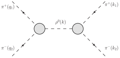
Figure 4: Elastic scattering of $\pi^{+}\pi^{-}$ with $\rho$ exchange in the $s$ channel.

Using the $\rho\pi\pi$ coupling (3.35) and the $\rho$ propagator (3.2) we get

$$\begin{split}\langle\pi^{+}(k_{1}),\pi^{-}(k_{2})|\mathcal{T}|\pi^{+}(q_{1}),\pi^{-}(q_{2})\rangle&=\frac{1}{4}\,g_{\rho\pi\pi}^{2}(k_{1}-k_{2})\cdot(q_{1}-q_{2})\Delta_{T}^{(\rho)}(k^{2})\,,\\ k=k_{1}+k_{2}&=q_{1}+q_{2}\,.\end{split}$$ (4.8)

With $\Delta_{T}^{(\rho)}(k^{2})$ from (4.6) all partial-wave unitarity relations are satisfied. But this is not the case if we use $\Delta_{T}^{(\rho)}(k^{2})$ from (3.5).

The careful reader of [22] will notice that the $\gamma V$ coupling used there looks very different from the VMD coupling (3.23). We shall, therefore, make some remarks on the relation of these different forms for the $\gamma V$ vertex. The following section deals more with theoretical concepts related to VMD and can be skipped by a reader only interested in practical applications of our model to high-energy reactions.

4.2 Different Forms of the $\gamma V$ Vertex and Approximate VMD

We shall now show that from the dispersion theoretic approach of [22] we can shed new light on the time-honoured VMD model. For this we present the essence of the arguments of [22] in Lagrangian language. Consider an effective field theory containing – to make the argument simple – just $\pi^{\pm}$ and $\rho^{0}$ meson fields. The assumptions of the model presented in section 4.1 of [22] can now be phrased as follows. It is assumed that there are couplings of the photon to the $\pi$ mesons and to the $\rho^{0}$ meson. The Lagrangian reads then

$$\begin{split}{\cal L}(x)=&\left(\partial_{\mu}\pi^{-}(x)\right)\partial^{\mu}\pi^{+}(x)-m_{\pi}^{2}\pi^{-}(x)\pi^{+}(x)\\ &+{\cal L}_{\rho^{0}}(x)+{\cal L}^{\prime}_{\gamma\pi\pi}(x)+{\cal L}^{\prime}_{\gamma\rho^{0}}(x)+{\cal L}^{\prime}_{\rho^{0}\pi\pi}(x)\,,\end{split}$$ (4.9)

where the $\rho^{0}$ kinetic term is

$${\cal L}_{\rho^{0}}(x)=-\frac{1}{2}\left(\partial_{\nu}\rho^{0}_{\mu}(x)\right)\left(\partial^{\nu}\rho^{0\mu}(x)\right)+\frac{1}{2}\left(\partial_{\mu}\rho^{0\mu}(x)\right)^{2}+\frac{1}{2}m_{\rho}^{2}\rho^{0}_{\mu}(x)\rho^{0\mu}(x)$$ (4.10)

and the interaction parts are

$${\cal L}^{\prime}_{\gamma\pi\pi}(x) =-ie\big{(}\pi^{-}(x)\overleftrightarrow{\partial_{\mu}}\pi^{+}(x)\big{)}A^{\mu}(x)+e^{2}\pi^{-}(x)\pi^{+}(x)A^{\mu}(x)A_{\mu}(x)\,,$$ (4.11)

$${\cal L}^{\prime}_{\gamma\rho^{0}}(x) =-\frac{e}{2\gamma_{\rho}}\big{(}\partial_{\mu}\rho_{\nu}^{0}(x)-\partial_{\nu}\rho_{\mu}^{0}(x)\big{)}\big{(}\partial^{\mu}A^{\nu}(x)-\partial^{\nu}A^{\mu}(x)\big{)}\,,$$ (4.12)

$${\cal L}^{\prime}_{\rho^{0}\pi\pi}(x) =-\frac{i}{2}g_{\rho\pi\pi}\big{(}\pi^{-}(x)\overleftrightarrow{\partial_{\mu}}\pi^{+}(x)\big{)}\rho^{0\mu}(x)\,.$$ (4.13)

Here $A_{\mu}(x)$ is the photon vector potential. The $\gamma$-$\rho$ coupling constant $1/\gamma_{\rho}$ in (4.12) is related to $f_{\rho}$ used in [22] as follows

$$\frac{1}{\gamma_{\rho}}\equiv\frac{f_{\rho}}{m_{\rho}}\,.$$ (4.14)

Note that together with the standard kinetic term for the $\pi^{\pm}$ fields the coupling of the photon to $\pi^{\pm}$ and $\rho^{0}$ in (4.9) is perfectly gauge invariant. Clearly, the $\gamma\rho^{0}$ coupling in (4.12) looks very different from the standard VMD coupling (3.23). But we can rewrite (4.12) as

$${\cal L}^{\prime}_{\gamma\rho^{0}}(x)={\cal L}^{\prime(1)}_{\gamma\rho^{0}}(x)+{\cal L}^{\prime(2)}_{\gamma\rho^{0}}(x)+{\cal L}^{\prime(3)}_{\gamma\rho^{0}}(x)\,,$$ (4.15)

where

$${\cal L}^{\prime(1)}_{\gamma\rho^{0}}(x) =-\frac{e}{\gamma_{\rho}}m_{\rho}^{2}\rho_{\mu}^{0}(x)A^{\mu}(x)\,,$$ (4.16)

$${\cal L}^{\prime(2)}_{\gamma\rho^{0}}(x) =\frac{e}{\gamma_{\rho}}A^{\mu}(x)\big{[}(\square+m_{\rho}^{2})\rho_{\mu}^{0}(x)-\partial_{\mu}\partial^{\nu}\rho_{\nu}^{0}(x)\big{]}\,,$$ (4.17)

$${\cal L}^{\prime(3)}_{\gamma\rho^{0}}(x) =-\frac{e}{\gamma_{\rho}}\partial^{\mu}\big{[}A^{\nu}(x)(\partial_{\mu}\rho_{\nu}^{0}(x)-\partial_{\nu}\rho_{\mu}^{0}(x))\big{]}\,.$$ (4.18)

The term ${\cal L}^{\prime(1)}_{\gamma\rho^{0}}$ in (4.16) gives exactly the standard VMD coupling (3.23). The term ${\cal L}^{\prime(3)}_{\gamma\rho^{0}}$ in (4.18) is a total divergence and can be dropped. The term ${\cal L}^{\prime(2)}_{\gamma\rho^{0}}$ in (4.17) has the following properties. It vanishes on the $\rho^{0}$ mass shell. For instance, it does not contribute to the decay of an ‘on shell’ $\rho^{0}$ to $e^{+}e^{-}$; see figure 5.

Figure 5: Diagram for the decay $\rho^{0}\to e^{+}e^{-}$

For processes with a virtual $\rho^{0}$ meson next to the coupling (4.17) the latter will eat up the $\rho^{0}$ propagator. As an example let us consider the reaction

$$e^{+}(l_{1})+e^{-}(l_{2})\longrightarrow\pi^{+}(k_{1})+\pi^{-}(k_{2})$$ (4.19)

and calculate the corresponding amplitude at tree level using the Lagrangian (4.9).

With (4.9) to (4.17) we have to consider three diagrams, see figure 6, the ‘direct’ term due to ${\cal L}^{\prime}_{\gamma\pi\pi}$ and the terms with an intermediate virtual $\rho^{0}$ due to ${\cal L}^{\prime(1)}_{\gamma\rho^{0}}$ and ${\cal L}^{\prime(2)}_{\gamma\rho^{0}}$.

$$(a)$$

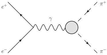
$$(b)$$

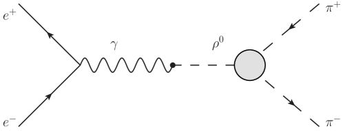
$$(c)$$

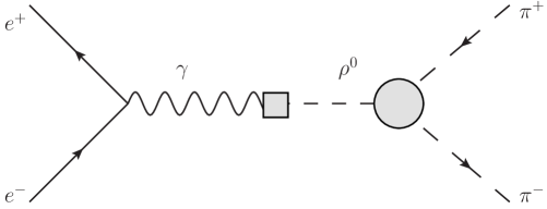
Figure 6: Tree level diagrams for $e^{+}e^{-}\to\pi^{+}\pi^{-}$ according to (4.9). Here (a), (b), and (c) correspond to the direct $\gamma\pi\pi$ coupling term ${\cal L}^{\prime}_{\gamma\pi\pi}$ (4.11), the $\gamma\rho^{0}$ coupling term ${\cal L}^{\prime(1)}_{\gamma\rho^{0}}$ (4.16), and the $\gamma\rho^{0}$ coupling term ${\cal L}^{\prime(2)}_{\gamma\rho^{0}}$ (4.17), respectively.

Using the $\rho^{0}$ propagator as obtained from (4.10) we find for the amplitudes corresponding to figures 6(a) to (c) the following:

$${\cal{M}}_{\text{direct}}=-ie^{2}(k_{1}-k_{2})^{\mu}\frac{1}{q^{2}}\,\bar{v}(l_{1})\gamma_{\mu}u(l_{2})\,,$$ (4.20)

$$\begin{split}{\cal{M}}_{\gamma\rho^{0}}^{(1)}&=-\frac{i}{2}g_{\rho\pi\pi}(k_{1}-k_{2})^{\mu}i\Delta_{\mu\nu}^{(\rho)}(q)\left(-i\frac{e}{\gamma_{\rho}}m_{\rho}^{2}\right)\left(\frac{-ig^{\nu\lambda}}{q^{2}}\right)\bar{v}(l_{1})ie\gamma_{\lambda}u(l_{2})\\ &=-ie^{2}\frac{1}{2}g_{\rho\pi\pi}\frac{(-m_{\rho}^{2})}{q^{2}-m_{\rho}^{2}}\frac{1}{\gamma_{\rho}}(k_{1}-k_{2})^{\mu}\frac{1}{q^{2}}\bar{v}(l_{1})\gamma_{\mu}u(l_{2})\,,\end{split}$$ (4.21)

$$\begin{split}{\cal{M}}_{\gamma\rho^{0}}^{(2)}&=-\frac{i}{2}g_{\rho\pi\pi}(k_{1}-k_{2})^{\mu}i\Delta_{\mu\kappa}^{(\rho)}(q)\frac{ie}{\gamma_{\rho}}\left[(-q^{2}+m_{\rho}^{2})\delta_{\nu}^{\kappa}+q^{\kappa}q_{\nu}\right]\left(\frac{-ig^{\nu\lambda}}{q^{2}}\right)\bar{v}(l_{1})ie\gamma_{\lambda}u(l_{2})\\ &=ie^{2}\frac{1}{2}g_{\rho\pi\pi}\frac{1}{\gamma_{\rho}}(k_{1}-k_{2})^{\mu}\frac{1}{q^{2}}\bar{v}(l_{1})\gamma_{\mu}u(l_{2})\,.\end{split}$$ (4.22)

In (4.20) to (4.22) we have set

$$q=l_{1}+l_{2}=k_{1}+k_{2}\,.$$ (4.23)

Indeed, in ${\cal M}^{(2)}_{\gamma\rho^{0}}$ the $\rho^{0}$-pole is cancelled. This means that ${\cal L}^{\prime(2)}_{\gamma\rho}$ does not provide a term where the photon couples to a $\rho^{0}$ meson which then interacts with the pion, as one would expect from figure 6(c), but in fact a direct coupling of the photon to the pions without intermediate $\rho^{0}$. This opens the possibility of having a partial or even complete cancellation between ${\cal M}_{\text{direct}}$ (4.20) and ${\cal M}^{(2)}_{\gamma\rho^{0}}$ (4.22). The VMD hypothesis assumes indeed that this cancellation is complete which requires

$$\frac{1}{2}\,g_{\rho\pi\pi}\,\frac{1}{\gamma_{\rho}}=1\,.$$ (4.24)

This tree level calculation above is only meant to give an understanding how the various forms of the $\gamma\rho^{0}$ vertex are related. Including self-energy corrections in the $\rho^{0}$ propagator we find that the diagram of figure 6(c) due to $\mathcal{L}^{\prime(2)}_{\gamma\rho^{0}}$ gives a ‘direct’ term plus a correction to the diagram of figure 6(b), that is, to the term due to $\mathcal{L}^{\prime(1)}_{\gamma\rho^{0}}$. From the rigorous dispersion theoretic analysis in [22] where VMD is not assumed we get, using the parameters from Table 4 (Fit III) there, the following:

$$g_{\rho\pi\pi}=11.51\pm 0.07\,,\quad f_{\rho}=155.4\pm 1.7\,\mbox{MeV}\,,\quad m_{\rho}=773.7\pm 0.4\,\mbox{MeV}\,.$$ (4.25)

This leads, with (4.14), to

$$\frac{1}{2}\,g_{\rho\pi\pi}\,\frac{1}{\gamma_{\rho}}=\frac{1}{2}\,g_{\rho\pi\pi}\,\frac{f_{\rho}}{m_{\rho}}=1.16\pm 0.01\,,$$ (4.26)

$$\frac{4\pi}{\gamma_{\rho}^{2}}=4\pi\left(\frac{f_{\rho}}{m_{\rho}}\right)^{2}=0.507\pm 0.011\,.$$ (4.27)

We see from (4.26) that the VMD relation (4.24) is, in this case, satisfied to an accuracy of around $15\%$. From (4.27) we get a value for $4\pi/\gamma^{2}_{\rho}$ which is well compatible with the one used in (3.25) which is taken from eq. (5.3) of [9].

To summarise: we have seen that the gauge invariant $\gamma\rho^{0}$ coupling ${\cal L}^{\prime}_{\gamma\rho^{0}}$ (4.12) contains the standard VMD $\gamma\rho^{0}$ coupling term ${\cal L}^{\prime(1)}_{\gamma\rho^{0}}$ (4.16) plus a term ${\cal L}^{\prime(2)}_{\gamma\rho^{0}}$ (4.17) which, effectively, describes a direct coupling of the photons to pions without intermediate $\rho^{0}$. In strict VMD this latter term exactly cancels the contribution from the original direct coupling ${\cal L}^{\prime}_{\gamma\pi\pi}$.

4.3 General VMD Hypothesis

In view of the above discussion, we think that the general VMD hypothesis can be stated as follows. We have for the coupling of the photon to light hadrons, that is, hadrons made from $u,d$, and $s$ quarks, the following Lagrangian, comprising a direct term without intermediate vector mesons and a coupling with intermediate vector mesons $V=\rho^{0},\omega,\phi$:

$${\cal L}^{\prime}(x)={\cal L}^{\prime}_{\gamma,\mathrm{direct}}(x)+\sum_{V=\rho^{0},\omega,\phi}{\cal L}^{\prime}_{\gamma V}(x)\,,$$ (4.28)

where for $V=\rho^{0},\omega,\phi$

$$\begin{split}{\cal L}^{\prime}_{\gamma V}(x)&=-\frac{e}{2\gamma_{V}}(\partial_{\mu}V_{\nu}(x)-\partial_{\nu}V_{\mu}(x))(\partial^{\mu}A^{\nu}(x)-\partial^{\nu}A^{\mu}(x))\\ &={\cal L}^{\prime(1)}_{\gamma V}(x)+{\cal L}^{\prime(2)}_{\gamma V}(x)+{\cal L}^{\prime(3)}_{\gamma V}(x)\,.\end{split}$$ (4.29)

Here the $\gamma_{V}$ are defined in (3.23), (3.25) and ${\cal L}^{\prime(i)}_{\gamma V}$ are defined as in (4.15) to (4.18) with $\rho^{0}$ replaced by $V$. The strict VMD hypothesis amounts to assuming that the coupling ${\cal L}^{\prime(2)}_{\gamma\rho^{0}}+{\cal L}^{\prime(2)}_{\gamma\omega}+{\cal L}^{\prime(2)}_{\gamma\phi}$ – which in fact is effectively a direct $\gamma$-hadron coupling – precisely cancels the term ${\cal L}^{\prime}_{\gamma,\mathrm{direct}}$ in (4.28). Note that the remaining coupling, the standard VMD one (3.23), which amounts to setting in (4.28) ${\cal L}^{\prime}={\cal L}^{\prime(1)}_{\gamma\rho^{0}}+{\cal L}^{\prime(1)}_{\gamma\omega}+{\cal L}^{\prime(1)}_{\gamma\phi}$, will only be gauge invariant if the $\rho^{0},\omega$, and $\phi$ fields are divergence free. It is, indeed, well known that with the standard VMD coupling (3.23) one has to be very careful in order to maintain gauge invariance in calculations.

Of course, it is also well known that the VMD model only gives approximate results. For soft reactions involving real photons these are typically correct at the $10\%$ to $20\%$ level. See, for instance, (4.24) and (4.26) and the extensive discussions of VMD in relation to experiments in [9], [33] and [23]. Keeping this limited accuracy of VMD relations in mind we shall, in the present work, use the standard VMD couplings (3.23) for simplicity. But we shall always maintain strict gauge invariance since our vertices of section 3 incorporate the divergence condition $\partial^{\mu}V_{\mu}(x)=0$ for the vector meson fields. We note that with our description of the pomeron as an effective spin $2$ exchange there is no problem in maintaining this divergence condition also for the ${\mathbbm{P}}\rho\rho$ vertex; see (3.47). Using VMD with the coupling (3.23) we get from this perfectly gauge invariant ${\mathbbm{P}}\gamma\rho$ and ${\mathbbm{P}}\gamma\gamma$ vertices. This is quite a non-trivial result.

5 Tensor Mesons

In this section we discuss the vertices and the propagator for the tensor meson $f_{2}\equiv f_{2}(1270)$. We also make a few remarks on the $a_{2}\equiv a_{2}(1320)$ meson.

5.1 $f_{2}\to\pi\pi$

For the decays $f_{2}\to\pi^{+}\pi^{-}$ and $f_{2}\to\pi^{0}\pi^{0}$ there is only one invariant amplitude. It can be obtained from the following effective interaction Lagrangian $(M_{0}=1$ GeV):

$$\begin{split}{\cal L}_{f_{2}\pi\pi}^{\prime}(x)=&\,\frac{1}{2M_{0}}g_{f_{2}\pi\pi}\phi_{\kappa\lambda}(x)\left(g^{\kappa\mu}g^{\lambda\nu}-\frac{1}{4}g^{\kappa\lambda}g^{\mu\nu}\right)\\ &\times\sum_{a=1}^{3}\left[\frac{1}{2}\pi_{a}(x)\partial_{\mu}\partial_{\nu}\pi_{a}(x)+\frac{1}{2}(\partial_{\mu}\partial_{\nu}\pi_{a}(x))\pi_{a}(x)-(\partial_{\mu}\pi_{a}(x))(\partial_{\nu}\pi_{a}(x))\right]\,.\end{split}$$ (5.1)

Here $\phi_{\kappa\lambda}$ is the $f_{2}$ field for which we require, since it corresponds to a neutral spin 2 particle,

$$\phi_{\kappa\lambda}=\phi_{\lambda\kappa}=\phi_{\kappa\lambda}^{\dagger}\,.$$ (5.2)

The $\pi_{a}$ ($a=1,2,3$) are the pion fields and we have

$$\begin{split}\pi^{\pm}(x)&=\frac{1}{\sqrt{2}}\,(\pi_{1}(x)\mp i\pi_{2}(x))\,,\\ \pi^{0}(x)&=\pi_{3}(x)\,.\end{split}$$ (5.3)

The coupling (5.1) gives the $f_{2}\pi\pi$ vertex (3.37) where we have added a form factor taking into account that a variation of the coupling with the off-shellness of the $f_{2}$ must be expected. A convenient parametrisation of such a form factor is the exponential form

$$F^{(f_{2}\pi\pi)}(k^{2})=\exp\left(-\frac{k^{2}-m_{f_{2}}^{2}}{\Lambda^{2}}\right)$$ (5.4)

with $\Lambda$ a parameter of the order 1 GeV. Here the normalisation condition

$$F^{(f_{2}\pi\pi)}(m_{f_{2}}^{2})=1$$ (5.5)

is clearly satisfied.

From (3.37) we find easily for an ‘on-shell’ $f_{2}$ ($k^{2}=m_{f_{2}}^{2}$)

$$\Gamma(f_{2}\to\pi^{0}\pi^{0})=\frac{1}{2}\Gamma(f_{2}\to\pi^{+}\pi^{-})=\frac{m_{f_{2}}}{960\pi}|g_{f_{2}\pi\pi}|^{2}\bigg{(}\frac{m_{f_{2}}}{M_{0}}\bigg{)}^{2}\bigg{(}1-\frac{4m_{\pi}^{2}}{m_{f_{2}}^{2}}\bigg{)}^{5/2}.$$ (5.6)

With $\Gamma_{f_{2}}$ from (3.9) and

$$\frac{\Gamma(f_{2}\to\pi\pi)}{\Gamma_{f_{2}}}=(84.8_{-1.2}^{+2.4})\%$$ (5.7)

from [20] we get

$$\left|g_{f_{2}\pi\pi}\right|=9.26\pm 0.15\,.$$ (5.8)

With the arguments presented later in section 7.1 we conclude that $g_{f_{2}\pi\pi}$ should be positive. Thus, we get finally as our best estimate, given in (3.38),

$$g_{f_{2}\pi\pi}=9.26\pm 0.15\,.$$ (5.9)

5.2 $f_{2}$ Propagator

The propagator of a tensor field $\phi_{\mu\nu}(x)=\phi_{\nu\mu}(x)=\phi_{\mu\nu}^{\dagger}(x)$ is defined as

$$\Delta^{(T)}_{\mu\nu,\kappa\lambda}(k)=\frac{1}{i}\int d^{4}x\,e^{ikx}\langle 0|\mathrm{T}^{*}(\phi_{\mu\nu}(x)\phi_{\kappa\lambda}(0))|0\rangle$$ (5.10)

where $\mathrm{T}^{*}$ is the covariantised T product. Let us first consider a free field corresponding to a tensor particle of mass $m_{f_{2}}$. To construct a basis for the polarisation tensors of such a particle of momentum $k$, $k^{2}=m_{f_{2}}^{2}$, $k^{0}>0$, we proceed as follows.

We consider $\vec{k}\neq 0$ and introduce orthonormal vectors $\vec{e}_{1},\vec{e}_{2},\vec{e}_{3}$ with

$$(\vec{e}_{1}\times\vec{e}_{2})\cdot\vec{e}_{3}=1\,,\qquad\vec{e}_{3}\parallel\vec{k}$$ (5.11)

and define

$$\epsilon^{(\pm)\mu}=\mp\frac{1}{\sqrt{2}}\begin{pmatrix}0\\ \vec{e}_{1}\pm i\vec{e}_{2}\end{pmatrix},\qquad\epsilon^{(0)\mu}=\frac{1}{m_{f_{2}}}\begin{pmatrix}|\vec{k}|\\ \vec{e}_{3}k^{0}\end{pmatrix}.$$ (5.12)

A basis for the polarisation tensors of our tensor particle is given by

$$\begin{split}\epsilon^{(m)\mu\nu}(k)=&\sum_{m_{1},m_{2}}\langle 1,m_{1};1,m_{2}|2,m\rangle\epsilon^{(m_{1})\mu}(k)\epsilon^{(m_{2})\nu}(k)\,,\\ &m=-2,...,2\,,\quad m_{i}=\pm 1,0\,,\quad i=1,2\,.\end{split}$$ (5.13)

Here $\langle 1,m_{1};1,m_{2}|2,m\rangle$ are the usual Clebsch-Gordan coefficients. We have then

$$\big{(}\epsilon_{\mu\nu}^{(m)}(k)\big{)}^{*}\epsilon^{(n)\mu\nu}(k)=\delta_{mn}\,.$$ (5.14)

From (5.13) we get the spin sum as

$$\sum_{m=-2}^{2} \epsilon_{\mu\nu}^{(m)}(k)\left(\epsilon_{\kappa\lambda}^{(m)}(k)\right)^{*}=\frac{1}{2}\left(-g_{\mu\kappa}+\frac{k_{\mu}k_{\kappa}}{m_{f_{2}}^{2}}\right)\left(-g_{\nu\lambda}+\frac{k_{\nu}k_{\lambda}}{m_{f_{2}}^{2}}\right)$$ (5.15)

$$+\frac{1}{2}\left(-g_{\mu\lambda}+\frac{k_{\mu}k_{\lambda}}{m_{f_{2}}^{2}}\right)\left(-g_{\nu\kappa}+\frac{k_{\nu}k_{\kappa}}{m_{f_{2}}^{2}}\right)-\frac{1}{3}\left(-g_{\mu\nu}+\frac{k_{\mu}k_{\nu}}{m_{f_{2}}^{2}}\right)\left(-g_{\kappa\lambda}+\frac{k_{\kappa}k_{\lambda}}{m_{f_{2}}^{2}}\right)\,.$$

The free propagator reads

$$\Delta^{(T)}_{\mu\nu,\kappa\lambda} (k)|_{\textrm{free}}=\frac{1}{k^{2}-m_{f_{2}}^{2}+i\epsilon}\left\{\frac{1}{2}\left(-g_{\mu\kappa}+\frac{k_{\mu}k_{\kappa}}{m_{f_{2}}^{2}}\right)\left(-g_{\nu\lambda}+\frac{k_{\nu}k_{\lambda}}{m_{f_{2}}^{2}}\right)\right.$$ (5.16)

$$\left.+\frac{1}{2}\left(-g_{\mu\lambda}+\frac{k_{\mu}k_{\lambda}}{m_{f_{2}}^{2}}\right)\left(-g_{\nu\kappa}+\frac{k_{\nu}k_{\kappa}}{m_{f_{2}}^{2}}\right)-\frac{1}{3}\left(-g_{\mu\nu}+\frac{k_{\mu}k_{\nu}}{m_{f_{2}}^{2}}\right)\left(-g_{\kappa\lambda}+\frac{k_{\kappa}k_{\lambda}}{m_{f_{2}}^{2}}\right)\right\}\,.$$

This is well known; see for instance [34, 35, 36, 37, 38, 39].

The full propagator (5.10) with $\phi_{\mu\nu}$ equal to the $f_{2}$ field should develop the resonance structure due to the $f_{2}$. But this structure should only appear in the true spin 2 part of the propagator (5.10). Thus, we must now discuss the spin decomposition of the full propagator for $k^{0}>0$, $k^{2}>0$. This is analogous to the decomposition of the vector propagator into transverse (spin 1) and longitudinal (spin 0) parts; see section 4.

The tensor-field propagator (5.10) contains, in general, spin 2 and spin 1 parts, and a $2\times 2$ matrix as spin 0 part. The spin 1 and the spin 0 parts are due to the divergence of the field, $\partial^{\mu}\phi_{\mu\nu}(x)$, and to $\partial^{\mu}\partial^{\nu}\phi_{\mu\nu}(x)$ and $g^{\mu\nu}\phi_{\mu\nu}(x)$, respectively. Thus, we can write down an expansion of the full propagator (5.10) in terms of tensors $P^{(i)}$, in essence projectors on the various spin components, times invariant functions $\Delta^{(i)}(k^{2})$:

$$\Delta^{(T)}_{\mu\nu,\kappa\lambda}(k)=P^{(2)}_{\mu\nu,\kappa\lambda}(k)\Delta^{(2)}(k^{2})+P^{(1)}_{\mu\nu,\kappa\lambda}(k)\Delta^{(1)}(k^{2})+\sum_{a,b=1}^{2}P^{(0,ab)}_{\mu\nu,\kappa\lambda}(k)\Delta^{(0)}_{ab}(k^{2})\,.$$ (5.17)

Here the spin 2 projector reads as in (5.15) but with $m_{f_{2}}^{2}$ replaced by $k^{2}+i\epsilon$,

$$\begin{split}P^{(2)}_{\mu\nu,\kappa\lambda}(k)=&\frac{1}{2}\left(-g_{\mu\kappa}+\frac{k_{\mu}k_{\kappa}}{k^{2}+i\epsilon}\right)\left(-g_{\nu\lambda}+\frac{k_{\nu}k_{\lambda}}{k^{2}+i\epsilon}\right)\\ &+\frac{1}{2}\left(-g_{\mu\lambda}+\frac{k_{\mu}k_{\lambda}}{k^{2}+i\epsilon}\right)\left(-g_{\nu\kappa}+\frac{k_{\nu}k_{\kappa}}{k^{2}+i\epsilon}\right)\\ &-\frac{1}{3}\left(-g_{\mu\nu}+\frac{k_{\mu}k_{\nu}}{k^{2}+i\epsilon}\right)\left(-g_{\kappa\lambda}+\frac{k_{\kappa}k_{\lambda}}{k^{2}+i\epsilon}\right)\,.\end{split}$$ (5.18)

The other tensors $P^{(1)}$ and $P^{(0,ab)}$ are given explicitly in appendix A. For the tensor field corresponding to the $f_{2}$ meson, the $f_{2}$ pole should only appear in the invariant function $\Delta^{(2)}(k^{2})$. In appendix A we present an analysis of $\Delta^{(2)}(k^{2})$ along similar lines as done for $\Delta_{T}^{(\rho)}(k^{2})$ in [22] and section 4. The result is as follows where we set $k^{2}=s$:

$$\left[\Delta^{(2)}(s)\right]^{-1}=-m_{f_{2}}^{2}+s+s\left[R_{f_{2}}(s)-R_{f_{2}}(m_{f_{2}}^{2})\right]+i\,\mathrm{Im}\,B_{f_{2}}(s)\,,$$ (5.19)

with

$$\mathrm{Im}\,B_{f_{2}}(s) =\frac{\Gamma_{f_{2}}}{\Gamma(f_{2}\to\pi\pi)}\frac{1}{320\pi}\left|\frac{g_{f_{2}\pi\pi}F^{(f_{2}\pi\pi)}(s)}{M_{0}}\right|^{2}s^{2}\left(1-\frac{4m_{\pi}^{2}}{s}\right)^{\frac{5}{2}}\theta(s-4m_{\pi}^{2})\,,$$ (5.20)

$$R_{f_{2}}(s) =\frac{s}{\pi}\,\mbox{V.\,P.}\int_{4m_{\pi}^{2}}^{\infty}ds^{\prime}\,\frac{\mathrm{Im}\,B_{f_{2}}(s^{\prime})}{s^{\prime 2}(s^{\prime}-s)}\,.$$ (5.21)

Here V. P. means again the principal value prescription. A good representation of the $f_{2}$ propagator for, say, $0<k^{2}<10\,\mbox{GeV}^{2}$ should then be given by

$$i\Delta^{(f_{2})}_{\mu\nu,\kappa\lambda}(k)=iP^{(2)}_{\mu\nu,\kappa\lambda}(k)\Delta^{(2)}(k^{2})\,.$$ (5.22)

This is the propagator listed in (3.6). Terms of the full tensor-field propagator (5.17) corresponding to spin 1 and spin 0 should not appear in (5.22) since these parts have nothing to do with the $f_{2}$ meson.

5.3 $f_{2}\to\gamma\gamma$

We discuss first the decay of an ‘on-shell’ $f_{2}$ to two photons

$$f_{2}(k,\epsilon)\longrightarrow\gamma(k_{1},\epsilon_{\gamma,1})+\gamma(k_{2},\epsilon_{\gamma,2})$$ (5.23)

where $k,k_{1},k_{2}$ are the momenta, $\epsilon$ is the polarisation tensor of the $f_{2}$ and $\epsilon_{\gamma,1},\epsilon_{\gamma,2}$ are the polarisation vectors of the photons. Due to Bose symmetry of the photons and gauge invariance only two invariant amplitudes are allowed for (5.23). The corresponding $f_{2}\gamma\gamma$ vertex is given in (3.39) where for an ‘on-shell’ $f_{2}$ and real photons all form factors equal 1. The coupling term generating this vertex is

$$\begin{split}{\cal L}_{f_{2}\gamma\gamma}^{\prime}=\left[a_{f_{2}\gamma\gamma}(\partial_{\kappa}F_{\mu\nu})(\partial_{\lambda}F^{\mu\nu})+b_{f_{2}\gamma\gamma}F_{\mu\kappa}F_{\;\lambda}^{\mu}\right]\left(g^{\kappa\kappa^{\prime}}g^{\lambda\lambda^{\prime}}-\frac{1}{4}g^{\kappa\lambda}g^{\kappa^{\prime}\lambda^{\prime}}\right)\phi_{\kappa^{\prime}\lambda^{\prime}}\end{split}$$ (5.24)

where $F_{\mu\nu}=\partial_{\mu}A_{\nu}-\partial_{\nu}A_{\mu}$ is the photon field-strength tensor.

From (3.39) we get for the ${\cal T}$-matrix elements of (5.23) in the $f_{2}$ rest system where $\vec{k}_{2}=-\vec{k_{1}}$

$$\begin{split}\langle\gamma(\vec{k}_{1},\epsilon_{\gamma,1}^{(+)}),\gamma(-\vec{k}_{1},\epsilon_{\gamma,2}^{(+)})|{\cal T}|f_{2}(\epsilon^{(0)})\rangle&=\langle\gamma(\vec{k}_{1},\epsilon_{\gamma,1}^{(-)}),\gamma(-\vec{k}_{1},\epsilon_{\gamma,2}^{(-)})|{\cal T}|f_{2}(\epsilon^{(0)})\rangle\\ &=\frac{m_{f_{2}}^{4}}{\sqrt{6}}a_{f_{2}\gamma\gamma}\,,\end{split}$$ (5.25)

$$\begin{split}\langle\gamma(\vec{k}_{1},\epsilon_{\gamma,1}^{(+)}),\gamma(-\vec{k}_{1},\epsilon_{\gamma,2}^{(-)})|{\cal T}|f_{2}(\epsilon^{(2)})\rangle&=\langle\gamma(\vec{k}_{1},\epsilon_{\gamma,1}^{(-)}),\gamma(-\vec{k}_{1},\epsilon_{\gamma,2}^{(+)})|{\cal T}|f_{2}(\epsilon^{(-2)})\rangle\\ &=m_{f_{2}}^{2}b_{f_{2}\gamma\gamma}\,.\end{split}$$ (5.26)

Here $\epsilon^{(m)}$ are the polarisation tensors of the $f_{2}$ at rest. These are constructed as in (5.11) to (5.13) with coordinate vectors $\vec{e}_{1},\vec{e}_{2},\vec{e}_{3}$ but choosing $\vec{e}_{3}=\vec{k}_{1}/|\vec{k}_{1}|$ as quantisation axis. The $\epsilon^{(\pm)}_{\gamma,i}$ ($i=1,2$) are the usual polarisation vectors of the photons. In the coordinate system considered we have

$$\epsilon_{\gamma,1}^{(\pm)\mu}=\mp\frac{1}{\sqrt{2}}\begin{pmatrix}0\\ \vec{e_{1}}\pm i\vec{e_{2}}\end{pmatrix},\qquad\epsilon_{\gamma,2}^{(\pm)\mu}=\mp\frac{1}{\sqrt{2}}\begin{pmatrix}0\\ \vec{e_{1}}\mp i\vec{e_{2}}\end{pmatrix}.$$ (5.27)

From (5.25) and (5.26) we see that $a_{f_{2}\gamma\gamma}$ and $b_{f_{2}\gamma\gamma}$ parametrise the so-called helicity zero and helicity two $f_{2}\to\gamma\gamma$ amplitudes, respectively. In the basis $\epsilon^{(m)},\epsilon^{(n_{i})}_{\gamma,i}$ ($i=1,2$) these are the only non-zero matrix elements. From this we get the decay rate

$$\Gamma(f_{2}\to\gamma\gamma)=\frac{m_{f_{2}}}{80\pi}\left[\frac{1}{6}m_{f_{2}}^{6}|a_{f_{2}\gamma\gamma}|^{2}+m_{f_{2}}^{2}|b_{f_{2}\gamma\gamma}|^{2}\right]\,.$$ (5.28)

To obtain numbers for $a_{f_{2}\gamma\gamma}$ and $b_{f_{2}\gamma\gamma}$ we use the values

$$\begin{split}&\Gamma(f_{2}\to\gamma\gamma)=(3.14\pm 0.20)\,\mbox{keV}\,,\\ &\text{helicity zero contribution }\approx 13\%\>\mbox{of}\>\Gamma(f_{2}\to\gamma\gamma)\,,\end{split}$$ (5.29)

as quoted for the preferred solution A in [40]. From this we obtain with the fine-structure constant $\alpha$

$$\frac{1}{6}|m_{f_{2}}^{3}a_{f_{2}\gamma\gamma}|^{2}+|m_{f_{2}}b_{f_{2}\gamma\gamma}|^{2}=(11.62\pm 0.74)\alpha^{2}$$ (5.30)

and for the couplings

$$|a_{f_{2}\gamma\gamma}|=\frac{e^{2}}{4\pi}1.45~{}\text{GeV}^{-3}\,,\qquad|b_{f_{2}\gamma\gamma}|=\frac{e^{2}}{4\pi}2.49~{}\text{GeV}^{-1}$$ (5.31)

with an estimated error of around $5\%$. From the arguments presented in section 7.2 below we conclude that we should have

$$a_{f_{2}\gamma\gamma}>0\,,\qquad b_{f_{2}\gamma\gamma}>0\,.$$ (5.32)

From (5.31) and (5.32) we get the numbers quoted in (3.40).

For off-shell $f_{2}$’s coupling to on- or off-shell photons we will again have to consider form factors. These are included in (3.39). Strictly speaking, this vertex should come with a single form factor $\tilde{F}^{(f_{2}\gamma\gamma)}(k^{2},k_{1}^{2},k_{2}^{2})$. We assume that it can be approximated by a factorised expression

$$\tilde{F}^{(f_{2}\gamma\gamma)}(k^{2},k_{1}^{2},k_{2}^{2})\approx F_{M}(k_{1}^{2})F_{M}(k_{2}^{2})F^{(f_{2}\gamma\gamma)}(k^{2})\,.$$ (5.33)

For lack of other information we will further set

$$F^{(f_{2}\gamma\gamma)}(k^{2})=F^{(f_{2}\pi\pi)}(k^{2})\,;$$ (5.34)

see (5.4).

Finally we have compared our vertices for $f_{2}\pi\pi$ and $f_{2}\gamma\gamma$ in (3.37) and (3.39), respectively, to the ones used in [39]. For on-shell $f_{2}$’s we find a one to one correspondence. But we note that our $f_{2}\gamma\gamma$ vertex is strictly gauge invariant everywhere. That is, we get from (3.21) and (3.39)

$$\begin{split}&k_{1}^{\mu}\Gamma_{\mu\nu\kappa\lambda}^{(f_{2}\gamma\gamma)}(k_{1},k_{2})=0\,,\\ &k_{2}^{\nu}\Gamma_{\mu\nu\kappa\lambda}^{(f_{2}\gamma\gamma)}(k_{1},k_{2})=0\,.\end{split}$$ (5.35)

This must be so since our coupling Lagrangian (5.24) is strictly gauge invariant.

5.4 $a_{2}\to\gamma\gamma$

The analysis of the vertices and the propagator of the $a_{2}\equiv a_{2}(1320)$ meson could be done along the same lines as for the $f_{2}$. But we leave this for future work. Here we limit ourselves to making some remarks on the decay $a_{2}\to\gamma\gamma$ which is the analogue of $f_{2}\to\gamma\gamma$ treated in section 5.3. The $a_{2}\gamma\gamma$ vertex function is as in (3.39) with the constants $a_{f_{2}\gamma\gamma}$ and $b_{f_{2}\gamma\gamma}$ replaced by $a_{a_{2}\gamma\gamma}$ and $b_{a_{2}\gamma\gamma}$, respectively, which gives (3.41). The decay rate is

$$\Gamma(a_{2}\to\gamma\gamma)=\frac{m_{a_{2}}}{80\pi}\bigg{\{}\frac{1}{6}m_{a_{2}}^{6}|a_{a_{2}\gamma\gamma}|^{2}+m_{a_{2}}^{2}|b_{a_{2}\gamma\gamma}|^{2}\bigg{\}}\,.$$ (5.36)

From [20] we find

$$m_{a_{2}}=1318.3_{-0.6}^{+0.5}~{}\text{MeV}\,,\quad\Gamma_{a_{2}}=107\pm 5~{}\text{MeV}\,,\quad\frac{\Gamma(a_{2}\to\gamma\gamma)}{\Gamma_{a_{2}}}=(9.4\pm 0.7)\times 10^{-6}\,.$$ (5.37)

This gives

$$\frac{1}{6}|m_{a_{2}}^{3}a_{a_{2}\gamma\gamma}|^{2}+|m_{a_{2}}b_{a_{2}\gamma\gamma}|^{2}=(3.60\pm 0.32)\alpha^{2}$$ (5.38)

which is roughly a factor $3$ smaller than the corresponding quantity for the $f_{2}$; see (5.30). We discuss these coupling constants further in section 7.2 below.

6 Exchanges with Charge Conjugation $C\!=\!+1$ and $C\!=\!-1$ in Nucleon-Nucleon Scattering

Let us consider $pp$ and $\bar{p}p$ elastic scattering

$$p(p_{1})+p(p_{2}) \longrightarrow p(p^{\prime}_{1})+p(p^{\prime}_{2})\,,$$ (6.1)

$$\bar{p}(p_{1})+p(p_{2}) \longrightarrow\bar{p}(p^{\prime}_{1})+p(p^{\prime}_{2})\,.$$ (6.2)

The standard kinematic variables are

$$\begin{split}&s=(p_{1}+p_{2})^{2}\,,\quad t=(p_{1}-p_{1}^{\prime})^{2}\,,\quad u=(p_{1}-p_{2}^{\prime})^{2}\,,\\ &\nu=\frac{1}{4}(s-u)=\frac{1}{4}(p_{1}+p_{1}^{\prime})\cdot(p_{2}+p_{2}^{\prime})\,.\end{split}$$ (6.3)

The ${\cal T}$-matrix elements for the reactions (6.1) and (6.2) can be expanded as follows

$$\langle p(p_{1}^{\prime}),p(p_{2}^{\prime})|{\cal T}|p(p_{1}),p(p_{2})\rangle =\bar{u}_{\alpha^{\prime}}(p_{1}^{\prime})\bar{u}_{\beta^{\prime}}(p_{2}^{\prime})\Gamma_{\alpha^{\prime}\alpha,\beta^{\prime}\beta}^{(pp)}(p_{1}^{\prime},p_{2}^{\prime},p_{1},p_{2})u_{\alpha}(p_{1})u_{\beta}(p_{2})\,,$$ (6.4)

$$\langle\bar{p}(p_{1}^{\prime}),p(p_{2}^{\prime})|{\cal T}|\bar{p}(p_{1}),p(p_{2})\rangle =\bar{v}_{\alpha}(p_{1})\bar{u}_{\beta^{\prime}}(p_{2}^{\prime})\Gamma_{\alpha\alpha^{\prime},\beta^{\prime}\beta}^{(\bar{p}p)}(p_{1}^{\prime},p_{2}^{\prime},p_{1},p_{2})v_{\alpha^{\prime}}(p_{1}^{\prime})u_{\beta}(p_{2})\,.$$ (6.5)

Here $\alpha,\beta,\alpha^{\prime},\beta^{\prime}\in\{1,\dots,4\}$ are Dirac indices. The substitution rule (crossing symmetry) requires

$$\Gamma_{\alpha\alpha^{\prime},\beta^{\prime}\beta}^{(\bar{p}p)}(p_{1}^{\prime},p_{2}^{\prime},p_{1},p_{2})=-\Gamma_{\alpha\alpha^{\prime},\beta^{\prime}\beta}^{(pp)}(-p_{1},p_{2}^{\prime},-p_{1}^{\prime},p_{2})\,.$$ (6.6)

The $16\times 16$ matrices $\Gamma^{(pp)}$ and $\Gamma^{(\bar{p}p)}$ can be expanded in the basis $\gamma^{\mu}\otimes\gamma_{\mu},~{}\gamma^{\mu}\gamma_{5}\otimes\gamma_{\mu}\gamma_{5},\dots,~{}{\mathbbm{1}}\otimes{\mathbbm{1}}$. The standard assumption is that at high energies only the $\gamma^{\mu}\otimes\gamma_{\mu}$ structure is relevant; see [15, 16, 17, 18, 9]. Following this assumption we can write

$$\Gamma_{\alpha^{\prime}\alpha,\beta^{\prime}\beta}^{(pp)}(p_{1}^{\prime},p_{2}^{\prime},p_{1},p_{2}) =T^{(pp)}(\nu,t)(\gamma^{\mu})_{\alpha^{\prime}\alpha}(\gamma_{\mu})_{\beta^{\prime}\beta}\,,$$ (6.7)

$$\Gamma_{\alpha\alpha^{\prime},\beta^{\prime}\beta}^{(\bar{p}p)}(p_{1}^{\prime},p_{2}^{\prime},p_{1},p_{2}) =T^{(\bar{p}p)}(\nu,t)(\gamma^{\mu})_{\alpha\alpha^{\prime}}(\gamma_{\mu})_{\beta^{\prime}\beta}\,.$$ (6.8)

Inserting (6.7) and (6.8) in (6.4) and (6.5), respectively, we get

$$\langle p(p_{1}^{\prime}),p(p_{2}^{\prime})|{\cal T}|p(p_{1}),p(p_{2})\rangle =T^{(pp)}(\nu,t)\,\bar{u}(p_{1}^{\prime})\gamma^{\mu}u(p_{1})\bar{u}(p_{2}^{\prime})\gamma_{\mu}u(p_{2})\,,$$ (6.9)

$$\langle\bar{p}(p_{1}^{\prime}),p(p_{2}^{\prime})|{\cal T}|\bar{p}(p_{1}),p(p_{2})\rangle =T^{(\bar{p}p)}(\nu,t)\,\bar{v}(p_{1})\gamma^{\mu}v(p_{1}^{\prime})\bar{u}(p_{2}^{\prime})\gamma_{\mu}u(p_{2})\,.$$ (6.10)

From QFT we know that, for fixed $t$, $T^{(pp)}(\nu,t)$ and $T^{(\bar{p}p)}(\nu,t)$ are boundary values of one analytic function in $\nu$, $A(\nu,t)$, with the cut structure shown in figure 7.

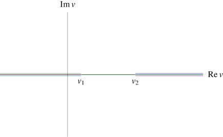
Figure 7: The analytic structure of the amplitude $A(\nu,t)$ for fixed $t$ in the interval (6.12).

The thresholds for the cuts are

$$\nu_{1}=m_{p}^{2}-\frac{1}{2}m_{\pi}^{2}-\frac{1}{4}t\,,\quad\nu_{2}=m_{p}^{2}+\frac{1}{4}t\,.$$ (6.11)

For

$$0\geq t>-m_{\pi}^{2}$$ (6.12)

we have

$$\nu_{1}<\nu_{2}$$ (6.13)

and the amplitude $A(\nu,t)$ is then real in the interval

$$\nu_{1}<\nu<\nu_{2}\,.$$ (6.14)

All this is easily seen from a study of the Landau singularities of the corresponding Feynman diagrams; see for instance [41] for an introduction to this topic. Then, for the $t$ interval (6.12), we have

$$A^{*}(\nu^{*},t)=A(\nu,t)\,.$$ (6.15)

The connection of $T^{(pp)},T^{(\bar{p}p)}$ to $A(\nu,t)$ is as follows. We have for real $\nu>\nu_{2}$

$$T^{(pp)}(\nu,t) =\lim_{\epsilon\to 0}A(\nu+i\epsilon,t)\,,$$ (6.16)

$$T^{(\bar{p}p)}(\nu,t) =-\lim_{\epsilon\to 0}A(-\nu-i\epsilon,t)\,.$$ (6.17)

So far all relations follow strictly from QFT. Now we shall invoke the Regge-pole model and assume that the amplitude $A(\nu,t)$ has a power behaviour in $\nu$ for $\nu\to\infty$. We shall treat $C=+1$ and $C=-1$ exchanges in turn.

6.1 Pomeron Exchange

There is a vast literature on the pomeron, for an overview see for instance [9]. Let us here just mention some investigations of the pomeron in perturbative QCD [42, 43, 44, 45, 46, 47, 48, 49] and in non-perturbative QCD [50, 51, 52, 53, 54, 55, 56, 57, 58, 59]. In the present paper we shall adopt a modest phenomenological approach following the Regge-pole model of Donnachie and Landshoff [16, 17, 18, 9].

Let us assume power behaviour for $A(\nu,t)$ for $\nu\to\infty$. The pomeron part of $A(\nu,t)$, corresponding to a $C=+1$ exchange, must be an odd function of $\nu$ for $\nu\to\infty$, see (6.16), (6.17), in order to give the same amplitudes for $pp$ and $\bar{p}p$ scattering. Therefore, our ansatz for the pomeron part of $A(\nu,t)$ reads

$$A^{\mathbbm{P}}(\nu,t)=f(t)\;2\alpha_{\mathbbm{P}}^{\prime}\;\nu\;\left[4\alpha_{\mathbbm{P}}^{\prime 2}(\nu_{2}-\nu)(\nu-\nu_{1})\right]^{\frac{1}{2}(\alpha_{\mathbbm{P}}(t)-2)}$$ (6.18)

with $f(t)$ a real function. Here $\alpha_{{\mathbbm{P}}}(t)$ is as in (3.11) and we have inserted suitable factors $\alpha^{\prime}_{{\mathbbm{P}}}=0.25$ GeV^-2 for dimensional reasons. The requirement that $A(\nu,t)$ is real in the interval (6.14) fixes the branches of the power functions to be taken in (6.18). That is, we require that $A^{{\mathbbm{P}}}(\nu,t)$ has exactly the cut structure shown in figure 7. We obtain then for $\nu$ real, $\nu\to\infty$ from (6.16) and (6.17)

$$T^{(pp){\mathbbm{P}}}(\nu,t)=T^{(\bar{p}p){\mathbbm{P}}}(\nu,t)=f(t)\,2\alpha_{\mathbbm{P}}^{\prime}\,\nu\,\left[4\alpha_{\mathbbm{P}}^{\prime 2}\nu^{2}e^{-i\pi}\right]^{\frac{1}{2}(\alpha_{\mathbbm{P}}(t)-2)}\,.$$ (6.19)

Setting now

$$f(t)=[3\beta_{{\mathbbm{P}}NN}F_{1}(t)]^{2}$$ (6.20)

with $\beta_{{\mathbbm{P}}NN}$ and $F_{1}(t)$ as in (3.43) and using in the high-energy limit

$$\nu\approx\frac{s}{2}$$ (6.21)

we get the celebrated Donnachie-Landshoff (DL) pomeron ansatz from (6.9), (6.10) and (6.19) to (6.21)

$$\langle p(p_{1}^{\prime}),p(p_{2}^{\prime})|{\cal T}|p(p_{1}),p(p_{2})\rangle\big{|}_{\mathbbm{P}}= \,i\,[3\beta_{{\mathbbm{P}}NN}F_{1}(t)]^{2}(-is\alpha_{\mathbbm{P}}^{\prime})^{\alpha_{\mathbbm{P}}(t)-1}$$

$$\times\bar{u}(p_{1}^{\prime})\gamma^{\mu}u(p_{1})\bar{u}(p_{2}^{\prime})\gamma_{\mu}u(p_{2})\,,$$ (6.22)

$$\langle\bar{p}(p_{1}^{\prime}),p(p_{2}^{\prime})|{\cal T}|\bar{p}(p_{1}),p(p_{2})\rangle\big{|}_{\mathbbm{P}}= \,i\,[3\beta_{{\mathbbm{P}}NN}F_{1}(t)]^{2}(-is\alpha_{\mathbbm{P}}^{\prime})^{\alpha_{\mathbbm{P}}(t)-1}$$

$$\times\bar{v}(p_{1})\gamma^{\mu}v(p_{1}^{\prime})\bar{u}(p_{2}^{\prime})\gamma_{\mu}u(p_{2})\,,$$ (6.23)

where the subscript ${\mathbbm{P}}$ indicates that we consider only the pomeron contribution. Here we have to set $-i=\exp(-i\pi/2)$ in the power functions.

The $\gamma^{\mu}\otimes\gamma_{\mu}$ structure in (6.1) and (6.1) suggests to consider the pomeron as some effective vector exchange. And, indeed, the DL pomeron is frequently called a ‘$C=+1$ photon’. But this presents severe problems from the point of view of QFT. A QFT vector will couple to the proton and the antiproton with opposite signs, giving a relative minus sign between (6.1) and (6.1). Of course, this is unacceptable since it would lead to the total cross sections for $pp$ and $\bar{p}p$ scattering having opposite signs. It is well known that a Regge-pole exchange as in (6.1) and (6.1) corresponds to the coherent sum of the exchanges of infinitely many spins. An explicit construction showing how (6.1) and (6.1) can be written in terms of a sum of quantum-field-theoretic exchanges with spin $2,4,6$ etc. can be found in section 6.2 of [51]. But infinite sums are in general cumbersome to handle. We shall show in the following how we can write the pomeron exchange in (6.1) and (6.1) as an effective spin $2$ exchange satisfying the standard QFT crossing requirements. In appendix B we show how this effective spin 2 exchange can again be written as a coherent sum of exchanges of spin 2, 4, 6, etc. We also explain there why the pomeron should have nothing to do with an effective spin 0 exchange.

Let us consider the reactions (6.1) and (6.2) in the c. m. system and let $\lambda_{1},\lambda_{2},\lambda^{\prime}_{1},\lambda^{\prime}_{2}\in\{1/2,-1/2\}$ be the helicities of the nucleons. For high energies, $s\to\infty$, we have

$$\bar{u}_{\lambda^{\prime}}(p^{\prime})\gamma^{\mu}u_{\lambda}(p)=\bar{v}_{\lambda}(p)\gamma^{\mu}v_{\lambda^{\prime}}(p^{\prime})\longrightarrow(p^{\prime}+p)^{\mu}\delta_{\lambda^{\prime}\lambda}\,.$$ (6.24)

Inserting this in (6.1) and (6.1) we get at high energies

$$\begin{split}\langle p(p_{1}^{\prime},\lambda_{1}^{\prime}),&\,p(p_{2}^{\prime},\lambda_{2}^{\prime})|{\cal T}|p(p_{1},\lambda_{1}),p(p_{2},\lambda_{2})\rangle\big{|}_{\mathbbm{P}}\\ =&\,\langle\bar{p}(p_{1}^{\prime},\lambda_{1}^{\prime}),p(p_{2}^{\prime},\lambda_{2}^{\prime})|{\cal T}|\bar{p}(p_{1},\lambda_{1}),p(p_{2},\lambda_{2})\rangle\big{|}_{\mathbbm{P}}\\ =&\,i\,2s\,[3\beta_{{\mathbbm{P}}NN}F_{1}(t)]^{2}(-is\alpha_{\mathbbm{P}}^{\prime})^{\alpha_{\mathbbm{P}}(t)-1}\delta_{\lambda_{1}^{\prime}\lambda_{1}}\delta_{\lambda_{2}^{\prime}\lambda_{2}}\,.\end{split}$$ (6.25)

We shall now show that exactly the same expression is obtained in the high-energy limit by considering the pomeron as a symmetric traceless rank $2$ tensor object

$${\mathbbm{P}}_{\mu\nu}(x)={\mathbbm{P}}_{\nu\mu}(x)\,,\qquad{\mathbbm{P}}_{\mu\nu}(x)g^{\mu\nu}=0$$ (6.26)

and making suitable ansätze for the ${\mathbbm{P}}pp$ vertex and the ${\mathbbm{P}}$ propagator. For the coupling Lagrangian of the tensor pomeron to proton and antiproton we make the ansatz

$${\cal L}^{\prime}_{{\mathbbm{P}}pp}(x)=-3\beta_{{\mathbbm{P}}NN}{\mathbbm{P}}_{\mu\nu}(x)\frac{i}{2}\bar{\psi}_{p}(x)\left[\gamma^{\mu}\stackrel{{\scriptstyle\leftrightarrow}}{{\partial^{\nu}}}+\gamma^{\nu}\stackrel{{\scriptstyle\leftrightarrow}}{{\partial^{\mu}}}-\frac{1}{2}g^{\mu\nu}\gamma^{\lambda}\stackrel{{\scriptstyle\leftrightarrow}}{{\partial_{\lambda}}}\right]\psi_{p}(x)$$ (6.27)

where $\psi_{p}(x)$ is the proton field operator. With this tensor coupling we get in the standard way from QFT the ${\mathbbm{P}}pp$ and ${\mathbbm{P}}\bar{p}\bar{p}$ vertices listed in (3.43). Our ansatz for the effective pomeron propagator is given in (3.10), (3.11). We get now the amplitudes and, using also (6.24), their expressions for large $s$ as follows:

$$\langle p(p_{1}^{\prime},\lambda_{1}^{\prime}), \,p(p_{2}^{\prime},\lambda_{2}^{\prime})|{\cal T}|p(p_{1},\lambda_{1}),p(p_{2},\lambda_{2})\rangle\big{|}_{\mathbbm{P}}$$

$$= \,i[3\beta_{{\mathbbm{P}}NN}F_{1}(t)]^{2}(-is\alpha_{\mathbbm{P}}^{\prime})^{\alpha_{\mathbbm{P}}(t)-1}$$

$$\times\bar{u}(p_{1}^{\prime},\lambda_{1}^{\prime})\left[\frac{1}{2}\gamma^{\mu}(p_{1}^{\prime}+p_{1})^{\nu}+\frac{1}{2}\gamma^{\nu}(p_{1}^{\prime}+p_{1})^{\mu}\right]u(p_{1},\lambda_{1})$$

$$\times\frac{1}{4s}\left(g_{\mu\kappa}g_{\nu\lambda}+g_{\mu\lambda}g_{\nu\kappa}-\frac{1}{2}g_{\mu\nu}g_{\kappa\lambda}\right)$$ (6.28)

$$\times\bar{u}(p_{2}^{\prime},\lambda_{2}^{\prime})\left[\frac{1}{2}\gamma^{\kappa}(p_{2}^{\prime}+p_{2})^{\lambda}+\frac{1}{2}\gamma^{\lambda}(p_{2}^{\prime}+p_{2})^{\kappa}\right]u(p_{2},\lambda_{2})$$

$$\!\!\!\!\!\!\!\!\xrightarrow[s\to\infty]{}i2s\,[3\beta_{{\mathbbm{P}}NN}F_{1}(t)]^{2}\;(-is\alpha_{\mathbbm{P}}^{\prime})^{\alpha_{\mathbbm{P}}(t)-1}\;\delta_{\lambda_{1}^{\prime}\lambda_{1}}\delta_{\lambda_{2}^{\prime}\lambda_{2}}\,,$$

$$\langle\bar{p}(p_{1}^{\prime},\lambda_{1}^{\prime}), \,p(p_{2}^{\prime},\lambda_{2}^{\prime})|{\cal T}|\bar{p}(p_{1},\lambda_{1}),p(p_{2},\lambda_{2})\rangle\big{|}_{\mathbbm{P}}$$

$$= \,i[3\beta_{{\mathbbm{P}}NN}F_{1}(t)]^{2}(-is\alpha_{\mathbbm{P}}^{\prime})^{\alpha_{\mathbbm{P}}(t)-1}$$

$$\times\bar{v}(p_{1},\lambda_{1})\left[\frac{1}{2}\gamma^{\mu}(p_{1}^{\prime}+p_{1})^{\nu}+\frac{1}{2}\gamma^{\nu}(p_{1}^{\prime}+p_{1})^{\mu}\right]v(p_{1}^{\prime},\lambda_{1}^{\prime})$$

$$\times\frac{1}{4s}\left(g_{\mu\kappa}g_{\nu\lambda}+g_{\mu\lambda}g_{\nu\kappa}-\frac{1}{2}g_{\mu\nu}g_{\kappa\lambda}\right)$$ (6.29)

$$\times\bar{u}(p_{2}^{\prime},\lambda_{2}^{\prime})\left[\frac{1}{2}\gamma^{\kappa}(p_{2}^{\prime}+p_{2})^{\lambda}+\frac{1}{2}\gamma^{\lambda}(p_{2}^{\prime}+p_{2})^{\kappa}\right]u(p_{2},\lambda_{2})$$

$$\!\!\!\!\!\!\!\!\xrightarrow[s\to\infty]{}i2s\,[3\beta_{{\mathbbm{P}}NN}F_{1}(t)]^{2}\;(-is\alpha_{\mathbbm{P}}^{\prime})^{\alpha_{\mathbbm{P}}(t)-1}\;\delta_{\lambda_{1}^{\prime}\lambda_{1}}\delta_{\lambda_{2}^{\prime}\lambda_{2}}\,.$$

Comparing (6.1) and (6.1) with (6.25) we find in the high energy limit complete agreement of the amplitudes calculated from our tensor-pomeron exchange with the standard DL amplitudes.

To summarise: in QFT a second rank tensor – like for gravity – gives the same sign for the coupling of particles and of antiparticles. Thus, our tensor pomeron has automatically the same coupling to $p$ and $\bar{p}$ as required by phenomenology. The resulting expressions for the amplitudes of elastic $pp$ and $\bar{p}p$ scattering are for $s\to\infty$ exactly as for the DL pomeron if the effective tensor-pomeron propagator and the couplings to the nucleons are chosen appropriately. This, together with the requirement of standard QFT structures, gives the justification a posteriori of the ansätze (3.10) and (3.43). Thus, one may ask if it pays to consider the pomeron as a tensor object. We shall show that once we consider the coupling of vector mesons to the pomeron, viewing the pomeron as a tensor object, presents enormous advantages, see section 7.2 below.

6.2 Odderon Exchange

The odderon – so far only seen clearly in theoretical papers – is a $C=-1$ exchange object. The corresponding amplitude $A^{\mathbbm{O}}(\nu,t)$ must be an even function of $\nu$ for $\nu\to\infty$ in order to give opposite signs for the amplitudes of $pp$ and $\bar{p}p$ scattering, see (6.16), (6.17), and it must again have the cut structure shown in figure 7. We make, as for the pomeron amplitude in (6.18), a power law ansatz for $A^{\mathbbm{O}}$,

$$A^{\mathbbm{O}}(\nu,t)=\big{[}3\beta_{{\mathbbm{O}}pp}F_{1}(t)\big{]}^{2}\eta_{\mathbbm{O}}\left[4\alpha_{\mathbbm{O}}^{\prime 2}(\nu_{2}-\nu)(\nu-\nu_{1})\right]^{\frac{1}{2}(\alpha_{\mathbbm{O}}(t)-1)},\quad\eta_{\mathbbm{O}}=\pm 1\,.$$ (6.30)

Here the coupling constant $\beta_{{\mathbbm{O}}pp}$ of dimension (mass)^-1, the factor $\eta_{\mathbbm{O}}$, and the trajectory function $\alpha_{\mathbbm{O}}(t)$ are, of course, unknown. They are to be taken as free parameters, hopefully to be determined some day by experiment. For dimensional reasons we have inserted the factor $\alpha^{\prime 2}_{{\mathbbm{O}}}$ in (6.30). In (3.17) we have made an ansatz for $\alpha_{\mathbbm{O}}(t)$ as a linear function of $t$

$$\alpha_{\mathbbm{O}}(t)=1+\epsilon_{\mathbbm{O}}+\alpha_{\mathbbm{O}}^{\prime}\,t\,.$$ (6.31)

For a ‘decent’ odderon we should have

$$|\epsilon_{\mathbbm{O}}|\ll 1\,.$$ (6.32)

Of course, the pomeron amplitude must dominate over the odderon one for $s\to\infty$ in order to ensure positive total $pp$ and $\bar{p}p$ cross sections. Thus, we must require

$$\epsilon_{\mathbbm{O}}\leq\epsilon_{\mathbbm{P}}\,;$$ (6.33)

see (3.11) and (3.17). The factor $\eta_{\mathbbm{O}}$ remains as a free parameter. For lack of other information we shall set $\alpha^{\prime}_{\mathbbm{O}}=\alpha^{\prime}_{\mathbbm{P}}=0.25\,\mbox{GeV}^{-2}$ as already listed in (3.17). We could also have used a scale factor different from $4\alpha^{\prime 2}_{\mathbbm{O}}$ in (6.30).

From (6.9) to (6.17) and (6.30) we obtain for high energies, $s\to\infty$,

$$\langle p(p_{1}^{\prime}),p(p_{2}^{\prime})|{\cal T}|p(p_{1}),p(p_{2})\rangle\big{|}_{\mathbbm{O}}= \,[3\beta_{{\mathbbm{O}}pp}F_{1}(t)]^{2}\eta_{\mathbbm{O}}(-is\alpha_{\mathbbm{O}}^{\prime})^{\alpha_{\mathbbm{O}}(t)-1}$$

$$\times\bar{u}(p_{1}^{\prime})\gamma^{\mu}u(p_{1})\bar{u}(p_{2}^{\prime})\gamma_{\mu}u(p_{2})\,,$$ (6.34)

$$\langle\bar{p}(p_{1}^{\prime}),p(p_{2}^{\prime})|{\cal T}|\bar{p}(p_{1}),p(p_{2})\rangle\big{|}_{\mathbbm{O}}= \,-[3\beta_{{\mathbbm{O}}pp}F_{1}(t)]^{2}\eta_{\mathbbm{O}}(-is\alpha_{\mathbbm{O}}^{\prime})^{\alpha_{\mathbbm{O}}(t)-1}$$

$$\times\bar{v}(p_{1})\gamma^{\mu}v(p_{1}^{\prime})\bar{u}(p_{2}^{\prime})\gamma_{\mu}u(p_{2})\,.$$ (6.35)

The relative minus sign between the $pp$ and the $\bar{p}p$ amplitudes is, of course, what is required for a $C=-1$ exchange. Thus we see that the odderon may be considered as an effective vector exchange in the sense of QFT. The corresponding coupling Lagrangian can be taken as

$${\cal L}_{{\mathbbm{O}}pp}^{\prime}(x)=-3M_{0}\beta_{{\mathbbm{O}}pp}{\mathbbm{O}}_{\mu}(x)\,\bar{\psi}_{p}(x)\gamma^{\mu}\psi_{p}(x)$$ (6.36)

where, for dimensional reason, we have inserted a factor $M_{0}\equiv 1\,\mbox{GeV}$ to make the coupling constant $M_{0}\beta_{{\mathbbm{O}}pp}$ dimensionless. From (6.36) we get in the standard way of QFT using also isospin symmetry the ${\mathbbm{O}}NN$ vertices (3.68). Choosing the effective odderon propagator according to (3.16), (3.17) gives then exactly the $pp$ and $\bar{p}p$ amplitudes (6.2) and (6.2), respectively.

To summarise: the odderon may be considered as effective vector exchange in the sense of QFT; see also [14] and sections 6.2 and 6.3 of [51]. This makes the odderon in some sense theoretically simpler than the pomeron. The odderon is supposed to be an isoscalar object. This fixes the ${\mathbbm{O}}nn$ and ${\mathbbm{O}}pp$ vertices in (3.68) to be equal. While the general structure of the effective odderon propagator (3.16) is fixed by the odderon’s vector property the details are completely open. A linear odderon trajectory (3.17) and a scale factor equal to $\alpha^{\prime}_{\mathbbm{O}}$ in the power law in (3.16) are just guesses to be confirmed or refuted by experiment.

Now we discuss the ${\mathbbm{O}}\gamma f_{2}$ coupling. For lack of other information we make for the effective coupling Lagrangian an ansatz in analogy to the one for $f_{2}\gamma\gamma$ in (5.24). We get then

$$\begin{split}{\cal L}_{{\mathbbm{O}}\gamma f_{2}}^{\prime}=&\left[a_{{\mathbbm{O}}\gamma f_{2}}(\partial_{\kappa}F_{\mu\nu})\partial_{\lambda}(\partial^{\mu}{\mathbbm{O}}^{\nu}-\partial^{\nu}{\mathbbm{O}}^{\mu})+b_{{\mathbbm{O}}\gamma f_{2}}F_{\mu\kappa}(\partial^{\mu}{\mathbbm{O}}_{\lambda}-\partial_{\lambda}{\mathbbm{O}}^{\mu})+(\kappa\leftrightarrow\lambda)\right]\\ &\times\left[g^{\kappa\kappa^{\prime}}g^{\lambda\lambda^{\prime}}-\frac{1}{4}g^{\kappa\lambda}g^{\kappa^{\prime}\lambda^{\prime}}\right]\phi_{\kappa^{\prime}\lambda^{\prime}}\,.\end{split}$$ (6.37)

Since we have a coupling involving one photon we define also coupling parameters where one factor of $e$ is taken out:

$$\hat{a}_{{\mathbbm{O}}\gamma f_{2}}=\frac{a_{{\mathbbm{O}}\gamma f_{2}}}{e}\qquad\hat{b}_{{\mathbbm{O}}\gamma f_{2}}=\frac{b_{{\mathbbm{O}}\gamma f_{2}}}{e}\,.$$ (6.38)

These $\hat{a}_{{\mathbbm{O}}\gamma f_{2}}$ and $\hat{b}_{{\mathbbm{O}}\gamma f_{2}}$ should then be of ‘normal’ size on the hadronic scale. The ${\mathbbm{O}}\gamma f_{2}$ vertex is easily obtained from (6.37) and is listed in (3.70) where appropriate form factors are included.

6.3 Reggeon Exchanges and Total Cross Sections

It is well known that in high-energy nucleon-nucleon scattering the subdominant terms after pomeron exchange are due to the reggeon exchanges $f_{2R},a_{2R},\omega_{R}$, and $\rho_{R}$; see for instance [9]. The reggeons $f_{2R}$ and $a_{2R}$ have charge conjugation $C=+1$, the reggeons $\omega_{R}$ and $\rho_{R}$ have $C=-1$. We construct, therefore, effective propagators and vertices for these $C=+1$ and $C=-1$ reggeons in complete analogy to those of the pomeron and the odderon, respectively.

Let us start with the $C=+1$ exchanges $f_{2R}$ and $a_{2R}$. We consider them as effective spin 2 exchanges. In analogy to pomeron exchange we make for the effective ${\mathbbm{R}}_{+}$ propagators and ${\mathbbm{R}}_{+}NN$ vertices (${\mathbbm{R}}_{+}=f_{2R},a_{2R}$) the ansätze (3.12), (3.49), and (3.51). Here we are taking into account that $f_{2R}$ is an isoscalar and $a_{2R}$ the third component of an isovector. We assume the so-called degeneracy to hold, that is, equal trajectories for $f_{2R}$ and $a_{2R}$. This is a good representation of the experimental findings; see [9]. The numbers quoted for this ${\mathbbm{R}}_{+}$ trajectory in (3.13) are taken from figure 2.8 and section 3.1 of [9]. The overall sign factor of the ${\mathbbm{R}}_{+}$ propagators can either be taken from experiment, see below, or from the signature-factor argument. For the latter see for instance (2.18) and (3.11) of [9] and (6.8.15) of [7]. The values for the couplings given in (3.50) and (3.52) are discussed below.

We treat the $C=-1$ reggeons ${\mathbb{R}}_{-}=\omega_{R},\rho_{R}$ as effective vector exchanges. Taking their isospin quantum numbers into account we obtain the propagators (3.14) and the vertices (3.59) and (3.61). The overall signs of the ${\mathbbm{R}}_{-}$ propagators can be determined from experiment or from the signature-factor argument. Again we assume degeneracy of the $\omega_{R}$ and $\rho_{R}$ trajectories and take the parameters of the ${\mathbbm{R}}_{-}$ trajectory from figure 2.8 and section 3.1 of [9]. As is shown there, the parameters of the ${\mathbbm{R}}_{+}$ and ${\mathbbm{R}}_{-}$ trajectories can be taken as equal. Of course, in our framework it would be easy to relax this assumption if so required by experiment. The values for the couplings in (3.60) and (3.62) are discussed below.

Now we can write down the expressions for the elastic amplitudes and cross sections for nucleon-nucleon scattering at high energies. Here we shall take into account the hadronic exchanges and neglect $\gamma$ exchange which is only relevant for very small $|t|$. Also the data which we shall consider refer only to the strong-interaction parts of the amplitudes. We get the following, using (6.24), for $pp$ and $pn$ scattering. For ease of writing we set for $p$ and $n$ also $N(I_{3})$ with $I_{3}=+1/2$ and $-1/2$, respectively.

$$\langle p(p_{1}^{\prime},\lambda_{1}^{\prime}),N(I_{3},p_{2}^{\prime},\lambda_{2}^{\prime})|{\cal T}|p (p_{1},\lambda_{1}),N(I_{3},p_{2},\lambda_{2})\rangle$$

$$=i\,2s\,\delta_{\lambda_{1}^{\prime}\lambda_{1}}\delta_{\lambda_{2}^{\prime}\lambda_{2}}[F_{1}(t)]^{2}\bigg{\{} \,(3\beta_{{\mathbbm{P}}NN})^{2}(-is\alpha_{\mathbbm{P}}^{\prime})^{\alpha_{\mathbbm{P}}(t)-1}$$

$$+\left[(g_{f_{2R}pp})^{2}+(-1)^{I_{3}-\frac{1}{2}}(g_{a_{2R}pp})^{2}\right]M_{0}^{-2}(-is\alpha_{{\mathbbm{R}}_{+}}^{\prime})^{\alpha_{{\mathbbm{R}}_{+}}(t)-1}$$

$$+\left[(g_{\omega_{R}pp})^{2}+(-1)^{I_{3}-\frac{1}{2}}(g_{\rho_{R}pp})^{2}\right]M_{-}^{-2}i\;(-is\alpha_{{\mathbbm{R}}_{-}}^{\prime})^{\alpha_{{\mathbbm{R}}_{-}}(t)-1}$$

$$+(3\beta_{{\mathbbm{O}}pp})^{2}(-i\eta_{\mathbbm{O}})(-is\alpha_{\mathbbm{O}}^{\prime})^{\alpha_{\mathbbm{O}}(t)-1}\bigg{\}}.$$ (6.39)

For $\bar{p}p$ and $\bar{p}n$ scattering we obtain

$$\langle\bar{p}(p_{1}^{\prime},\lambda_{1}^{\prime}),N(I_{3},p_{2}^{\prime},\lambda_{2}^{\prime})|{\cal T}|\bar{p} (p_{1},\lambda_{1}),N(I_{3},p_{2},\lambda_{2})\rangle$$

$$=i\,2s\,\delta_{\lambda_{1}^{\prime}\lambda_{1}}\delta_{\lambda_{2}^{\prime}\lambda_{2}}[F_{1}(t)]^{2}\bigg{\{} \,(3\beta_{{\mathbbm{P}}NN})^{2}(-is\alpha_{\mathbbm{P}}^{\prime})^{\alpha_{\mathbbm{P}}(t)-1}$$

$$+\left[(g_{f_{2R}pp})^{2}+(-1)^{I_{3}-\frac{1}{2}}(g_{a_{2R}pp})^{2}\right]M_{0}^{-2}(-is\alpha_{{\mathbbm{R}}_{+}}^{\prime})^{\alpha_{{\mathbbm{R}}_{+}}(t)-1}$$

$$-\left[(g_{\omega_{R}pp})^{2}+(-1)^{I_{3}-\frac{1}{2}}(g_{\rho_{R}pp})^{2}\right]M_{-}^{-2}i(-is\alpha_{{\mathbbm{R}}_{-}}^{\prime})^{\alpha_{{\mathbbm{R}}_{-}}(t)-1}$$

$$-(3\beta_{{\mathbbm{O}}pp})^{2}(-i\eta_{\mathbbm{O}})(-is\alpha_{\mathbbm{O}}^{\prime})^{\alpha_{\mathbbm{O}}(t)-1}\bigg{\}}.$$ (6.40)

For the total cross sections of $pp,pn,\bar{p}p$, and $\bar{p}n$ scattering we obtain from the optical theorem for high energies

$$\sigma_{\rm tot}(p, \,N(I_{3}))=\frac{1}{4s}\sum_{\lambda_{1},\lambda_{2}}\text{Im}\langle p(p_{1},\lambda_{1}),N(I_{3},p_{2},\lambda_{2})|{\cal T}|p(p_{1},\lambda_{1}),N(I_{3},p_{2},\lambda_{2})\rangle$$

$$=2\bigg{\{} (3\beta_{{\mathbbm{P}}NN})^{2}\cos\left[\frac{\pi}{2}(\alpha_{\mathbbm{P}}(0)-1)\right](s\alpha_{\mathbbm{P}}^{\prime})^{\alpha_{\mathbbm{P}}(0)-1}$$

$$+\left[(g_{f_{2R}pp})^{2}+(-1)^{I_{3}-\frac{1}{2}}(g_{a_{2R}pp})^{2}\right]M_{0}^{-2}\cos\left[\frac{\pi}{2}(\alpha_{{\mathbbm{R}}_{+}}(0)-1)\right](s\alpha_{{\mathbbm{R}}_{+}}^{\prime})^{\alpha_{{\mathbbm{R}}_{+}}(0)-1}$$

$$-\left[(g_{\omega_{R}pp})^{2}+(-1)^{I_{3}-\frac{1}{2}}(g_{\rho_{R}pp})^{2}\right]M_{-}^{-2}\cos\left[\frac{\pi}{2}\alpha_{{\mathbbm{R}}_{-}}(0)\right](s\alpha_{{\mathbbm{R}}_{-}}^{\prime})^{\alpha_{{\mathbbm{R}}_{-}}(0)-1}$$

$$+\eta_{\mathbbm{O}}(3\beta_{{\mathbbm{O}}pp})^{2}\cos\left[\frac{\pi}{2}\alpha_{{\mathbbm{O}}}(0)\right](s\alpha_{{\mathbbm{O}}}^{\prime})^{\alpha_{{\mathbbm{O}}}(0)-1}\bigg{\}},$$ (6.41)

$$\sigma_{\rm tot}(\bar{p}, \,N(I_{3}))$$

$$=2\bigg{\{} (3\beta_{{\mathbbm{P}}NN})^{2}\cos\left[\frac{\pi}{2}(\alpha_{\mathbbm{P}}(0)-1)\right](s\alpha_{\mathbbm{P}}^{\prime})^{\alpha_{\mathbbm{P}}(0)-1}$$

$$+\left[(g_{f_{2R}pp})^{2}+(-1)^{I_{3}-\frac{1}{2}}(g_{a_{2R}pp})^{2}\right]M_{0}^{-2}\cos\left[\frac{\pi}{2}(\alpha_{{\mathbbm{R}}_{+}}(0)-1)\right](s\alpha_{{\mathbbm{R}}_{+}}^{\prime})^{\alpha_{{\mathbbm{R}}_{+}}(0)-1}$$

$$+\left[(g_{\omega_{R}pp})^{2}+(-1)^{I_{3}-\frac{1}{2}}(g_{\rho_{R}pp})^{2}\right]M_{-}^{-2}\cos\left[\frac{\pi}{2}\alpha_{{\mathbbm{R}}_{-}}(0)\right](s\alpha_{{\mathbbm{R}}_{-}}^{\prime})^{\alpha_{{\mathbbm{R}}_{-}}(0)-1}$$

$$-\eta_{\mathbbm{O}}(3\beta_{{\mathbbm{O}}pp})^{2}\cos\left[\frac{\pi}{2}\alpha_{{\mathbbm{O}}}(0)\right](s\alpha_{{\mathbbm{O}}}^{\prime})^{\alpha_{{\mathbbm{O}}}(0)-1}\bigg{\}}.$$ (6.42)

In figures 3.1 and 3.2 of [9] the following fits to the experimental total cross sections are presented

$$\sigma_{\mathrm{tot}}(a,b)=X_{ab}\left(\frac{s}{M_{0}^{2}}\right)^{0.0808}+Y_{ab}\left(\frac{s}{M_{0}^{2}}\right)^{-0.4525}\,.$$ (6.43)

Here $(a,b)=(p,p),(p,n),(\bar{p},p),(\bar{p},n)$, and $M_{0}=1\,\mbox{GeV}$. The numbers given in [9] are

$$X_{ab}\equiv X=21.70\,\mbox{mb}\>\,\widehat{=}\>\,55.73\,\mbox{GeV}^{-2}$$ (6.44)

and for $Y_{ab}$ as listed in table 2.

$a$	$b$	$Y_{ab}$
$p$	$p$	56.08 mb	144.02 GeV-2
$p$	$n$	54.77 mb	140.66 GeV-2
$\bar{p}$	$p$	98.39 mb	252.68 GeV-2
$\bar{p}$	$n$	92.71 mb	238.10 GeV-2

Table 2: Values for $Y_{ab}$ in (6.43) from figures 3.1 and 3.2 of [9].

An odderon contribution is apparently not needed to fit these total cross section data. But we note that for $\alpha_{{\mathbbm{O}}}(0)\approx 1$ we have

$$\cos\left[\frac{\pi}{2}\alpha_{\mathbbm{O}}(0)\right]\approx 0\,.$$ (6.45)

Thus, as is well known, an odderon with $\alpha_{{\mathbbm{O}}}(0)\approx 1$ will hardly be visible in total cross sections; see (6.3) and (6.3).

Comparing now (6.3) and (6.3) with (6.43) we can first of all extract the intercepts of the pomeron, ${\mathbbm{R}}_{+}$, and ${\mathbbm{R}}_{-}$ trajectories,

$$\begin{split}\alpha_{\mathbbm{P}}(0)&=1+\epsilon_{\mathbbm{P}}=1.0808\,,\\ \alpha_{{\mathbbm{R}}_{+}}(0)=\alpha_{{\mathbbm{R}}_{-}}(0)&=1-0.4525=0.5475\,.\end{split}$$ (6.46)

These values are quoted in (3.11), (3.13) and (3.15). Furthermore, we get

$$(\beta_{{\mathbbm{P}}NN})^{2}=X\,\left[18\cos\left(\frac{\pi}{2}\epsilon_{\mathbbm{P}}\right)(M_{0}^{2}\alpha_{\mathbbm{P}}^{\prime})^{\epsilon_{\mathbbm{P}}}\right]^{-1},$$ (6.47)

$$(M_{0})^{-2}g_{f_{2R}pp}^{2}= \,[Y_{pp}+Y_{pn}+Y_{\bar{p}p}+Y_{\bar{p}n}]$$

$$\times\left[8\cos\left(\frac{\pi}{2}(\alpha_{{\mathbbm{R}}_{+}}(0)-1)\right)(M_{0}^{2}\alpha_{{\mathbbm{R}}_{+}}^{\prime})^{\alpha_{{\mathbbm{R}}_{+}}(0)-1}\right]^{-1},$$ (6.48)

$$(M_{0})^{-2}g_{a_{2R}pp}^{2}= \,[Y_{pp}-Y_{pn}+Y_{\bar{p}p}-Y_{\bar{p}n}]$$

$$\times\left[8\cos\left(\frac{\pi}{2}(\alpha_{{\mathbbm{R}}_{+}}(0)-1)\right)(M_{0}^{2}\alpha_{{\mathbbm{R}}_{+}}^{\prime})^{\alpha_{{\mathbbm{R}}_{+}}(0)-1}\right]^{-1},$$ (6.49)

$$(M_{-})^{-2}g_{\omega_{R}pp}^{2}= \,[-Y_{pp}-Y_{pn}+Y_{\bar{p}p}+Y_{\bar{p}n}]$$

$$\times\left[8\cos\left(\frac{\pi}{2}\alpha_{{\mathbbm{R}}_{-}}(0)\right)(M_{0}^{2}\alpha_{{\mathbbm{R}}_{-}}^{\prime})^{\alpha_{{\mathbbm{R}}_{-}}(0)-1}\right]^{-1},$$ (6.50)

$$(M_{-})^{-2}g_{\rho_{R}pp}^{2}= \,[-Y_{pp}+Y_{pn}+Y_{\bar{p}p}-Y_{\bar{p}n}]$$

$$\times\left[8\cos\left(\frac{\pi}{2}\alpha_{{\mathbbm{R}}_{-}}(0)\right)(M_{0}^{2}\alpha_{{\mathbbm{R}}_{-}}^{\prime})^{\alpha_{{\mathbbm{R}}_{-}}(0)-1}\right]^{-1}.$$ (6.51)

From (6.47) we get with $X$ from (6.44) and $\epsilon_{\mathbbm{P}}$, $\alpha^{\prime}_{\mathbbm{P}}$ from (3.11)

$$(\beta_{{\mathbbm{P}}NN})^{2}=3.49~{}\text{GeV}^{-2}\,.$$ (6.52)

Assuming now $\beta_{{\mathbbm{P}}NN}>0$ gives

$$\beta_{{\mathbbm{P}}NN}=1.87\,\mbox{GeV}^{-1}$$ (6.53)

as listed in (3.44). This is the standard DL value for $\beta_{{\mathbbm{P}}NN}$ given in [16, 17, 18]. Inserting the numerical values for $Y_{ab}$ from table 2 in (6.3) to (6.3) we get the results for the squared couplings listed in table 3. We can only give estimates for the errors on these numbers, maybe of order $5\%$ for the $f_{2R}$ and $\omega_{R}$ values and significantly larger for the $a_{2R}$ and $\rho_{R}$ values.

	[GeV-2]
$(M_{0})^{-2}g^{2}_{f_{2R}pp}$	121.95
$(M_{0})^{-2}g^{2}_{a_{2R}pp}$	2.82
$(M_{-})^{-2}g^{2}_{\omega_{R}pp}$	37.65
$(M_{-})^{-2}g^{2}_{\rho_{R}pp}$	2.05

Table 3: Numerical values for the squared couplings from (6.3) to (6.3) and table 2.

We shall now assume

$$g_{f_{2R}pp}>0\,,\qquad g_{a_{2R}pp}>0\,.$$ (6.54)

From table 3 we get then

$$g_{f_{2R}pp}=11.04\,,\qquad g_{a_{2R}pp}=1.68\,.$$ (6.55)

These are the values adopted in (3.50) and (3.52), respectively.

To obtain numerical estimates for the couplings $g_{\omega_{R}pp}$ and $g_{\rho_{R}pp}$ themselves, as well as for the mass parameter $M_{-}$ we proceed as follows. We consider the electromagnetic form factors of proton and neutron at zero momentum transfer and assume the VMD model with $V=\omega,\rho$ to hold at this kinematic point. In the corresponding diagrams shown in figure 8 we have the $\gamma V$ couplings which are known, see (3.23) and (3.25), and the couplings $Vpp$ and $Vnn$. We shall now assume that these latter couplings are the same as the reggeon couplings $V_{R}pp$, $V_{R}nn~{}(V=\omega,\rho)$:

$$g_{Vpp}\approx g_{V_{R}pp}\,,\quad g_{Vnn}\approx g_{V_{R}nn}\quad\mbox{for $V=\omega,\rho$}\,.$$ (6.56)

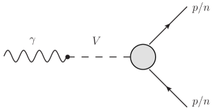
Figure 8: VMD diagrams for the nucleon electromagnetic form factors ($V=\omega,\rho$).

We obtain then from the diagrams of figure 8 and the known charges of $p$ and $n$ with the isospin relations $g_{\rho_{R}nn}=-g_{\rho_{R}pp}$ and $g_{\omega_{R}nn}=g_{\omega_{R}pp}$

$$\frac{1}{\gamma_{\rho}}g_{\rho_{R}pp}+\frac{1}{\gamma_{\omega}}g_{\omega_{R}pp}=1\,,\qquad-\frac{1}{\gamma_{\rho}}g_{\rho_{R}pp}+\frac{1}{\gamma_{\omega}}g_{\omega_{R}pp}=0\,;$$ (6.57)

so that

$$g_{\omega_{R}pp}=\frac{1}{2}\gamma_{\omega}=\sqrt{\pi}\bigg{(}\frac{4\pi}{\gamma_{\omega}^{2}}\bigg{)}^{-1/2}\,,\qquad g_{\rho_{R}pp}=\frac{1}{2}\gamma_{\rho}=\sqrt{\pi}\bigg{(}\frac{4\pi}{\gamma_{\rho}^{2}}\bigg{)}^{-1/2}\,.$$ (6.58)

With the numbers for $4\pi/\gamma^{2}_{V}$ from (3.25) this gives

$$g_{\omega_{R}pp} =8.65\pm 0.15\,,$$ (6.59)

$$g_{\rho_{R}pp} =2.52\pm 0.06\,,$$ (6.60)

$$\frac{g_{\omega_{R}pp}}{g_{\rho_{R}pp}} =3.43\pm 0.10\,.$$ (6.61)

This has to be compared to

$$\left|\frac{g_{\omega_{R}pp}}{g_{\rho_{R}pp}}\right|=4.29$$ (6.62)

from table 3 where our error estimate is at least $10\%$. The central values for $|g_{\omega_{R}pp}/g_{\rho_{R}pp}|$ from (6.61) and (6.62) differ only by $\approx 20\%$, a typical accuracy for VMD arguments. This gives credence to our assumption (6.56). We shall, therefore, fix the signs of $g_{\omega_{R}pp}$ and $g_{\rho_{R}pp}$ from the VMD relations (6.58), (6.59), (6.60). Since $(M_{-})^{2}g^{2}_{\omega_{R}pp}$ is much bigger and better determined than $(M_{-})^{2}g^{2}_{\rho_{R}pp}$ from table 3 we shall in the following take for $g_{\omega_{R}pp}$ the VMD value from (6.59) and calculate $M_{-}$ from table 3. This gives

$$M_{-}=\frac{g_{\omega_{R}pp}}{\sqrt{37.65}}\,\mbox{GeV}=1.41\,\mbox{GeV}$$ (6.63)

which is very reasonable for a hadronic mass parameter. From table 3 we get then

$$g_{\rho_{R}pp}=2.02\,.$$ (6.64)

The values for $M_{-}$ from (6.63), for $g_{\omega_{R}pp}$ from (6.59), and for $g_{\rho_{R}pp}$ from (6.64) are taken as default values for the parameters of the propagators and vertices in (3.15), (3.60), and (3.62), respectively.

In this section we have obtained default values for our coupling parameters by considering just the imaginary parts of the forward-scattering amplitudes (6.3), (6.3). Of course, the next step should be to confront the model with the extensive knowledge about elastic scattering; for reviews see for instance [9, 11, 60]. For recent work on exclusive central production where also elastic scattering is treated see [61]. Also the TOTEM results [62] from LHC should be taken into account. They have been discussed in the context of Regge theory for example in [63]. We leave the discussion of these issues in view of our model for future work.

7 Pion-Proton and $\rho$-Proton Scattering

7.1 Pion-Proton Scattering

We consider here the reactions

$$\pi^{\pm}(p_{1})+p(p_{2},\lambda_{2})\longrightarrow\pi^{\pm}(p^{\prime}_{1})+p(p^{\prime}_{2},\lambda^{\prime}_{2})$$ (7.1)

at high energies. Again we set

$$s=(p_{1}+p_{2})^{2}\,,\qquad t=(p_{1}-p^{\prime}_{1})^{2}\,.$$ (7.2)

The diagrams for these reactions with ${\mathbbm{P}},f_{2R},\rho_{R}$ and $\gamma$ exchange are shown in figure 2. We shall only consider the hadronic exchanges in the following. Note that $G$-parity invariance of strong interactions forbids $a_{2R}\pi\pi$, $\omega_{R}\pi\pi$, and ${\mathbbm{O}}\pi\pi$ vertices, cf. table 1. As in sections 6.1 and 6.3 we shall treat the pomeron and $f_{2R}$ exchanges as effective rank-2 tensor exchanges. The ${\mathbbm{P}}$ and $f_{2R}$ propagators are already constructed. It remains to construct the ${\mathbbm{P}}\pi\pi$ and $f_{2R}\pi\pi$ vertices. In analogy to ${\cal L}^{\prime}_{{\mathbbm{P}}pp}$ in (6.27) and ${\cal L}^{\prime}_{f_{2}\pi\pi}$ in (5.1) we make the following ansatz for the ${\mathbbm{P}}\pi\pi$ coupling Lagrangian

$$\begin{split}{\cal L}_{{\mathbbm{P}}\pi\pi}^{\prime}(x)=&2\beta_{{\mathbbm{P}}\pi\pi}{\mathbbm{P}}_{\kappa\lambda}(x)\left(g^{\kappa\mu}g^{\lambda\nu}-\frac{1}{4}g^{\kappa\lambda}g^{\mu\nu}\right)\\ &\times\sum_{a=1}^{3}\left[\frac{1}{2}\pi_{a}(x)\partial_{\mu}\partial_{\nu}\pi_{a}(x)+\frac{1}{2}(\partial_{\mu}\partial_{\nu}\pi_{a}(x))\pi_{a}(x)-(\partial_{\mu}\pi_{a}(x))(\partial_{\nu}\pi_{a}(x))\right]\,.\end{split}$$ (7.3)

This leads to the ${\mathbbm{P}}\pi\pi$ vertex (3.45). The coupling constant $\beta_{{\mathbbm{P}}\pi\pi}$ of dimension $\mathrm{mass}^{-1}$ will be determined below. Our ansatz for the $f_{2R}\pi\pi$ vertex is completely analogous to the ${\mathbbm{P}}\pi\pi$ vertex and is given in (3.53). For the $\rho_{R}\pi\pi$ vertex we can take the $\rho\pi\pi$ vertex (3.35) as a model. Our coupling Lagrangian reads (compare (4.13))

$${\cal L}_{\rho_{R}\pi\pi}^{\prime}=\frac{1}{2}g_{\rho_{R}\pi\pi}\;\rho_{R}^{\mu}(x)[i\pi^{+}(x)\overleftrightarrow{\partial_{\mu}}\pi^{-}(x)]\,.$$ (7.4)

This leads to the vertex (3.63) with $g_{\rho_{R}\pi\pi}$ to be determined below.

We are now ready to write down the amplitudes for the reactions (7.1). For high energies we find the following, using (6.24),

$$\begin{split}\langle\pi^{\pm}(p_{1}^{\prime}),p(p_{2}^{\prime},\lambda_{2}^{\prime})|{\cal T}|\pi^{\pm}(p_{1}),p(p_{2},&\,\lambda_{2})\rangle\\ =i\;2s\;\delta_{\lambda_{2}^{\prime}\lambda_{2}}F_{1}(t)F_{M}(t)\bigg{\{}&\,6\beta_{{\mathbbm{P}}\pi\pi}\beta_{{\mathbbm{P}}NN}(-is\alpha_{\mathbbm{P}}^{\prime})^{\alpha_{\mathbbm{P}}(t)-1}\\ &+\frac{1}{2}g_{f_{2R}\pi\pi}\;g_{f_{2R}pp}M_{0}^{-2}(-is\alpha_{{\mathbbm{R}}_{+}}^{\prime})^{\alpha_{{\mathbbm{R}}_{+}}(t)-1}\\ &\pm\frac{i}{2}g_{\rho_{R}\pi\pi}\;g_{\rho_{R}pp}M_{-}^{-2}(-is\alpha_{{\mathbbm{R}}_{-}}^{\prime})^{\alpha_{{\mathbbm{R}}_{-}}(t)-1}\bigg{\}}.\end{split}$$ (7.5)

From (7.5) we find via the optical theorem for large $s$

$$\begin{split}\sigma_{\rm tot}(\pi^{\pm},p)=&\,\frac{1}{2s}\sum_{\lambda_{2}}\text{Im}\,\langle\pi^{\pm}(p_{1}),p(p_{2},\lambda_{2})|{\cal T}|\pi^{\pm}(p_{1}),p(p_{2},\lambda_{2})\rangle\\ =&\,2\bigg{\{}6\beta_{{\mathbbm{P}}\pi\pi}\,\beta_{{\mathbbm{P}}NN}\cos\left[\frac{\pi}{2}(\alpha_{\mathbbm{P}}(0)-1)\right](s\alpha_{\mathbbm{P}}^{\prime})^{\alpha_{\mathbbm{P}}(0)-1}\\ &\hskip 14.22636pt+\frac{1}{2}g_{f_{2R}\pi\pi}\;g_{f_{2R}pp}M_{0}^{-2}\cos\left[\frac{\pi}{2}(\alpha_{{\mathbbm{R}}_{+}}(0)-1)\right](s\alpha_{{\mathbbm{R}}_{+}}^{\prime})^{\alpha_{{\mathbbm{R}}_{+}}(0)-1}\\ &\hskip 14.22636pt\mp\frac{1}{2}g_{\rho_{R}\pi\pi}\;g_{\rho_{R}pp}M_{-}^{-2}\cos\left[\frac{\pi}{2}\alpha_{{\mathbbm{R}}_{-}}(0)\right](s\alpha_{{\mathbbm{R}}_{-}}^{\prime})^{\alpha_{{\mathbbm{R}}_{-}}(0)-1}\bigg{\}}.\end{split}$$ (7.6)

In figure 3.1 of [9] the following fit to the experimental total cross sections $\sigma_{\text{tot}}(\pi^{\pm},p)$ is presented

$$\sigma_{\rm tot}(\pi^{\pm},p)=X_{\pi p}\bigg{(}\frac{s}{M_{0}^{2}}\bigg{)}^{0.0808}+Y_{\pi^{\pm}p}\bigg{(}\frac{s}{M_{0}^{2}}\bigg{)}^{-0.4525}\,.$$ (7.7)

Here

$$\begin{split}X_{\pi p}&=13.63~{}\text{mb}\;\widehat{=}\;35.00~{}\text{GeV}^{-2}\,,\\ Y_{\pi^{+}p}&=27.56~{}\text{mb}\;\widehat{=}\;70.78~{}\text{GeV}^{-2}\,,\\ Y_{\pi^{-}p}&=36.02~{}\text{mb}\;\widehat{=}\;92.51~{}\text{GeV}^{-2}\,.\end{split}$$ (7.8)

From (7.6) and (7.7) and with (3.11), (3.13), (3.15) we get

$$\beta_{{\mathbbm{P}}\pi\pi}\,\beta_{{\mathbbm{P}}NN} =X_{\pi p}\left[12\cos\left[\frac{\pi}{2}(\alpha_{\mathbbm{P}}(0)-1)\right](M_{0}^{2}\alpha_{\mathbbm{P}}^{\prime})^{\alpha_{\mathbbm{P}}(0)-1}\right]^{-1}\,,$$ (7.9)

$$(M_{0})^{-2}g_{f_{2R}\pi\pi}\;g_{f_{2R}pp} =(Y_{\pi^{+}p}+Y_{\pi^{-}p})\left[2\cos\left[\frac{\pi}{2}(\alpha_{{\mathbbm{R}}_{+}}(0)-1)\right](M_{0}^{2}\alpha_{{\mathbbm{R}}_{+}}^{\prime})^{\alpha_{{\mathbbm{R}}_{+}}(0)-1}\right]^{-1}\,,$$ (7.10)

$$(M_{-})^{-2}g_{\rho_{R}\pi\pi}\;g_{\rho_{R}pp} =(Y_{\pi^{-}p}-Y_{\pi^{+}p})\left[2\cos\left[\frac{\pi}{2}\alpha_{{\mathbbm{R}}_{-}}(0)\right](M_{0}^{2}\alpha_{{\mathbbm{R}}_{-}}^{\prime})^{\alpha_{{\mathbbm{R}}_{-}}(0)-1}\right]^{-1}.$$ (7.11)

With $X_{\pi p}$ and $Y_{\pi^{\pm}p}$ from (7.8) and the values for the pomeron and Regge trajectories from (3.11), (3.13), and (3.15) we get from (7.9) to (7.11)

$$\beta_{{\mathbbm{P}}\pi\pi}\,\beta_{{\mathbbm{P}}NN} =3.29~{}\text{GeV}^{-2}\,,$$ (7.12)

$$(M_{0})^{-2}g_{f_{2R}\pi\pi}\;g_{f_{2R}pp} =102.72~{}\text{GeV}^{-2}\,,$$ (7.13)

$$(M_{-})^{-2}g_{\rho_{R}\pi\pi}\;g_{\rho_{R}pp} =15.88~{}\text{GeV}^{-2}\,.$$ (7.14)

We can use (7.12) to (7.14) and the results of section 6.3 for the pomeron and reggeon couplings to the proton and extract the corresponding couplings to pions. From (7.12) we find with $\beta_{{\mathbbm{P}}NN}$ from (3.44)

$$\beta_{{\mathbbm{P}}\pi\pi}=1.76\,\mbox{GeV}^{-1}\,.$$ (7.15)

With $M_{-}=1.41\,\mbox{GeV}$ from (6.63), $g_{f_{2R}pp}$ from (3.50) and $g_{\rho_{R}pp}$ from (3.62) we find

$$g_{f_{2R}\pi\pi} =9.30\,,$$ (7.16)

$$g_{\rho_{R}\pi\pi} =15.63\,.$$ (7.17)

These are the default values listed in (3.46), (3.54) and (3.64), respectively.

Now we recall that from $\Gamma(f_{2}\to\pi\pi)$ we determined $|g_{f_{2}\pi\pi}|=9.26\pm 0.15$ in (5.8). This is surprisingly close to what we get from (7.16) identifying $g_{f_{2R}\pi\pi}$ and $g_{f_{2}\pi\pi}$. This motivates us to extract the sign of $g_{f_{2}\pi\pi}$ from this identification which leads to (5.9) and (3.38).

For $g_{\rho\pi\pi}$ (3.36) and $g_{\rho_{R}\pi\pi}$ (7.17) we find agreement in sign and in magnitude to $\approx 25\%$. Given the error on $g_{\rho_{R}\pi\pi}$ which should certainly be taken to be at least $10\%$ we find this result rather satisfactory. It gives again support to our hypothesis of relating ordinary and reggeon vertices.

7.2 $\rho^{0}$-Proton Scattering

In this section we consider elastic $\rho^{0}$-proton scattering:

$$\rho^{0}(p_{1},\epsilon_{1})+p(p_{2},\lambda_{2})\longrightarrow\rho^{0}(p^{\prime}_{1},\epsilon^{\prime}_{1})+p(p^{\prime}_{2},\lambda^{\prime}_{2})\,.$$ (7.18)

Here $\lambda_{2},\lambda^{\prime}_{2},\in\{1/2,-1/2\}$ are the proton helicities and $\epsilon_{1},\epsilon^{\prime}_{1}$ the $\rho^{0}$ polarisation vectors. Of course, the reaction (7.18) is hard to observe directly in experiments. But (7.18) will be an important ingredient in our study of photoproduction reactions in [19]. The diagrams for elastic $\rho p$ scattering at high energies are shown in figure 3. We are here interested in $\rho^{0}p$ scattering (7.18) where $C=-1$ exchange is forbidden. Also $a_{2R}$ exchange is forbidden by isospin invariance. We are left with ${\mathbbm{P}}$ and $f_{2R}$ exchange which – in our approach – are both treated as rank-two tensor exchanges. The general structure of the ${\mathbbm{P}}\rho\rho$ and the $f_{2R}\rho\rho$ vertices must, therefore, be as we found it for the $f_{2}\gamma\gamma$ vertex; see (3.39). This leads to our ansätze (3.47) and (3.55). The parameters listed in (3.48) and (3.56) will be discussed below. The amplitude for (7.18) is now easily written down. For large $s$ we find with (6.24)

$$\begin{split}\langle\rho^{0}(p_{1}^{\prime},\epsilon_{1}^{\prime}),p(p_{2}^{\prime},\lambda_{2}^{\prime})|{\cal T}|\rho^{0}(&\,p_{1},\epsilon_{1}),p(p_{2},\lambda_{2})\rangle\\ =-i\delta_{\lambda_{2}^{\prime}\lambda_{2}}\frac{1}{2s}F_{1}(t)F_{M}(t)&(\epsilon_{1}^{\prime\mu})^{*}\epsilon_{1}^{\nu}(p_{2}^{\prime}+p_{2})^{\kappa}(p_{2}^{\prime}+p_{2})^{\lambda}\\ \times\bigg{\{}\Gamma_{\mu\nu\kappa\lambda}^{(0)}(p_{1}^{\prime},-p_{1})&\left[6\beta_{{\mathbbm{P}}NN}a_{{\mathbbm{P}}\rho\rho}(-is\alpha_{\mathbbm{P}}^{\prime})^{\alpha_{\mathbbm{P}}(t)-1}\right.\\ &\left.+2M_{0}^{-1}g_{f_{2R}pp}\,a_{f_{2R}\rho\rho}(-is\alpha_{{\mathbbm{R}}_{+}}^{\prime})^{\alpha_{{\mathbbm{R}}_{+}}(t)-1}\right]\\ -\Gamma_{\mu\nu\kappa\lambda}^{(2)}(p_{1}^{\prime},-p_{1})&\left[3\beta_{{\mathbbm{P}}NN}b_{{\mathbbm{P}}\rho\rho}(-is\alpha_{\mathbbm{P}}^{\prime})^{\alpha_{\mathbbm{P}}(t)-1}\right.\\ &\left.+M_{0}^{-1}g_{f_{2R}pp}\,b_{f_{2R}\rho\rho}(-is\alpha_{{\mathbbm{R}}_{+}}^{\prime})^{\alpha_{{\mathbbm{R}}_{+}}(t)-1}\right]\bigg{\}}\,.\end{split}$$ (7.19)

Using the optical theorem we can calculate from (7.19) the total cross sections for $\rho^{0}$ mesons of definite helicities on unpolarised protons. Working in the c. m. system of the reaction (7.18) we define the polarisation vectors for $\rho^{0}$ of four-momentum $p_{1}=(p_{1}^{0},\vec{p}_{1})^{T}$ and helicity $m\in\{\pm 1,0\}$ as follows

$$\epsilon^{(\pm 1)\mu}=\mp\frac{1}{\sqrt{2}}\begin{pmatrix}0\\ \vec{e_{1}}\pm i\vec{e_{2}}\end{pmatrix}\,,\qquad\epsilon^{(0)\mu}=\frac{1}{m_{\rho}}\begin{pmatrix}|\vec{p_{1}}|\\ \vec{e_{3}}p_{1}^{0}\end{pmatrix}\,.$$ (7.20)

Here $\vec{e}_{1},\vec{e}_{2},\vec{e}_{3}$ are right-handed Cartesian basis vectors with $\vec{e}_{3}=\vec{p}_{1}/|\vec{p}_{1}|$. From (7.19) we get

$$\begin{split}\sigma_{\rm tot}&(\rho^{0}(\epsilon^{(m)}),p)=\frac{1}{2s}\sum_{\lambda_{2}}\text{Im}\langle\rho^{0}(p_{1},\epsilon^{(m)}),p(p_{2},\lambda_{2})|{\cal T}|\rho^{0}(p_{1},\epsilon^{(m)}),p(p_{2},\lambda_{2})\rangle\\ =&\,3\beta_{{\mathbbm{P}}NN}\left[2m_{\rho}^{2}\;a_{{\mathbbm{P}}\rho\rho}+(1-\delta_{m,0})b_{{\mathbbm{P}}\rho\rho}\right]\cos\left[\frac{\pi}{2}(\alpha_{\mathbbm{P}}(0)-1)\right](s\alpha_{\mathbbm{P}}^{\prime})^{\alpha_{\mathbbm{P}}(0)-1}\\ &+g_{f_{2R}pp}M_{0}^{-1}\left[2m_{\rho}^{2}a_{f_{2R}\rho\rho}+(1-\delta_{m,0})b_{f_{2R}\rho\rho}\right]\cos\left[\frac{\pi}{2}(\alpha_{{\mathbbm{R}}_{+}}(0)-1)\right](s\alpha_{{\mathbbm{R}}_{+}}^{\prime})^{\alpha_{{\mathbbm{R}}_{+}}(0)-1}\,.\end{split}$$ (7.21)

Note that in our approach the total cross sections for $\rho^{0}$ mesons with longitudinal $(m=0)$ and transverse $(m=\pm 1)$ polarisation are different.

In order to get estimates for the ${\mathbbm{P}}\rho\rho$ and $f_{2R}\rho\rho$ coupling constants we make the assumption that at high energies the total cross section for transversely polarised $\rho^{0}$ mesons equals the average of the $\pi^{+}p$ and $\pi^{-}p$ cross sections.
Assumption:

$$\sigma_{\rm tot}(\rho^{0}(\epsilon^{(m)}),p)=\frac{1}{2}\big{[}\sigma_{\rm tot}(\pi^{+},p)+\sigma_{\rm tot}(\pi^{-},p)\big{]}\qquad\text{for }m=\pm 1.$$ (7.22)

We can motivate (7.22) by a VMD argument. Let us calculate the total $\gamma p$ cross section from the VMD diagram in figure 9 taking into account only the $\rho^{0}$ contribution since the $\gamma\rho^{0}$ coupling is much larger than the $\gamma\omega$ and $\gamma\phi$ couplings; see (3.23) to (3.25).

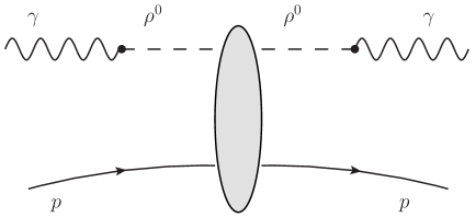
Figure 9: VMD diagram for $\gamma p$ forward scattering with intermediate $\rho^{0}$ meson.

Since real photons have only transverse polarisation we get from figure 9 with (3.23) and (3.3)

$$\sigma_{\rm tot}(\gamma,p)=\frac{e^{2}}{4\pi}\left(\frac{4\pi}{\gamma_{\rho}^{2}}\right)\frac{1}{2}\sum_{m=\pm 1}\sigma_{\rm tot}(\rho^{0}(\epsilon^{(m)}),p)\,.$$ (7.23)

In the spirit of VMD the cross section for on-shell $\rho^{0}$ mesons is to be inserted here. With the assumption (7.22) we should have, therefore,

$$\begin{split}\sigma_{\rm tot}(\gamma,p)&=\frac{e^{2}}{4\pi}\left(\frac{4\pi}{\gamma_{\rho}^{2}}\right)\frac{1}{2}\left[\sigma_{\rm tot}(\pi^{+},p)+\sigma_{\rm tot}(\pi^{-},p)\right]\\ &=3.6\times 10^{-3}\,\frac{1}{2}\left[\sigma_{\rm tot}(\pi^{+},p)+\sigma_{\rm tot}(\pi^{-},p)\right]\,.\end{split}$$ (7.24)

This relation is compared to data in figure 10.

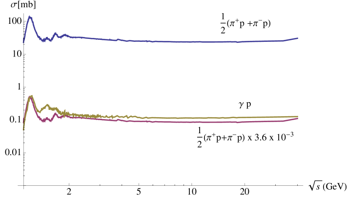
Figure 10: Data for $\frac{1}{2}\left(\sigma_{\rm tot}(\pi^{+},p)+\sigma_{\rm tot}(\pi^{-},p)\right)$ and rescaled by a factor $3.6\times 10^{-3}$ compared to $\sigma_{\rm tot}(\gamma,p)$ as function of the c. m. energy $\sqrt{s}$. Data are from [64], the $\pi^{\pm}p$ data have been interpolated for computing their average.

The agreement is quite reasonable. Note that $\sigma_{\rm tot}(\gamma,p)$ should be a little higher than the r. h. s. of (7.24) due to the contribution from $\omega$ and $\phi$ mesons in this energy range.

With the $\pi p$ total cross sections from (7.6) we obtain now from (7.21) and (7.22)

$$3\beta_{{\mathbbm{P}}NN}(2m_{\rho}^{2}a_{{\mathbbm{P}}\rho\rho}+b_{{\mathbbm{P}}\rho\rho}) =12\beta_{{\mathbbm{P}}NN}\;\beta_{{\mathbbm{P}}\pi\pi}\,,$$ (7.25)

$$g_{f_{2R}pp}M_{0}^{-1}(2m_{\rho}^{2}a_{f_{2R}\rho\rho}+b_{f_{2R}\rho\rho}) =g_{f_{2R}pp}\;g_{f_{2R}\pi\pi}M_{0}^{-2}\,.$$ (7.26)

From (7.25) and (7.15) we get

$$2m_{\rho}^{2}\;a_{{\mathbbm{P}}\rho\rho}+b_{{\mathbbm{P}}\rho\rho}=4\beta_{{\mathbbm{P}}\pi\pi}=7.04~{}\text{GeV}^{-1}\,.$$ (7.27)

This is the relation listed in (3.48). Combining (7.26) and (7.16) gives

$$2m_{\rho}^{2}\;a_{f_{2R}\rho\rho}+b_{f_{2R}\rho\rho}=M_{0}^{-1}g_{f_{2R}\pi\pi}=9.30~{}\text{GeV}^{-1}\,.$$ (7.28)

For the couplings $a_{f_{2R}\rho\rho}$ and $b_{f_{2R}\rho\rho}$ we can go a step further and give estimates for them individually. We shall assume that the couplings of the meson $f_{2}$ to $\rho^{0}\rho^{0}$ and of the reggeon $f_{2R}$ to $\rho^{0}\rho^{0}$ are equal:

$$a_{f_{2}\rho\rho}\approx a_{f_{2R}\rho\rho}\,,\qquad b_{f_{2}\rho\rho}\approx b_{f_{2R}\rho\rho}\,.$$ (7.29)

Here $a_{f_{2}\rho\rho}$ and $b_{f_{2}\rho\rho}$ are defined as the $f_{2}\gamma\gamma$ couplings in (3.39) but for $\rho^{0}$ in place of $\gamma$. The next step is to relate the $f_{2}\rho\rho$ couplings to the $f_{2}\gamma\gamma$ couplings using VMD. Taking into account only the $\rho^{0}$ meson, that is, neglecting contributions from the $\omega$ and $\phi$ mesons we get for $f_{2}\to\gamma\gamma$ the VMD diagram in figure 11. With (3.23), (3.25) and (3.39) this gives

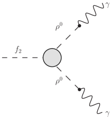
Figure 11: VMD diagram for $f_{2}\to\gamma\gamma$ with intermediate $\rho^{0}$.

$$a_{f_{2}\gamma\gamma}=\frac{e^{2}}{\gamma_{\rho}^{2}}a_{f_{2}\rho\rho}\,\qquad b_{f_{2}\gamma\gamma}=\frac{e^{2}}{\gamma_{\rho}^{2}}b_{f_{2}\rho\rho}\,.$$ (7.30)

With (7.29) and the numbers from (3.40) we get as estimates

$$a_{f_{2}\rho\rho} =a_{f_{2R}\rho\rho}=a_{f_{2}\gamma\gamma}\left(\alpha\frac{4\pi}{\gamma_{\rho}^{2}}\right)^{-1}=2.92~{}\text{GeV}^{-3}\,,$$ (7.31)

$$b_{f_{2}\rho\rho} =b_{f_{2R}\rho\rho}=b_{f_{2}\gamma\gamma}\left(\alpha\frac{4\pi}{\gamma_{\rho}^{2}}\right)^{-1}=5.02~{}\text{GeV}^{-1}\,.$$ (7.32)

Note that we have assumed here

$$a_{f_{2}\gamma\gamma}>0\,,\qquad b_{f_{2}\gamma\gamma}>0\,.$$ (7.33)

From (7.31) and (7.32) we get

$$2m_{\rho}^{2}a_{f_{2R}\rho\rho}+b_{f_{2R}\rho\rho}=8.52~{}\text{GeV}^{-1}$$ (7.34)

which agrees with (7.28) to better than $10\%$. We take this as supporting the above sign assumptions (7.33) for $a_{f_{2}\gamma\gamma}$ and $b_{f_{2}\gamma\gamma}$. The values for $a_{f_{2R}\rho\rho}$ from (7.31) and for $b_{f_{2R}\rho\rho}$ from (7.32) are taken as default values in (3.56).

For the coupling parameters of $\rho_{R}\rho^{0}f_{2}$ in (3.66) we take again as estimates

$$a_{\rho_{R}\rho^{0}f_{2}}\approx a_{f_{2R}\rho\rho}\,,\qquad b_{\rho_{R}\rho^{0}f_{2}}\approx b_{f_{2R}\rho\rho}\,.$$ (7.35)

With (7.31) and (7.32) this gives the default values quoted in (3.67).

The $f_{2}$ can also couple to $\omega\omega$ and $\omega_{R}\omega$. We have neglected this in our VMD argument above, see figure 11, since the $\gamma$-$\omega$ coupling is much smaller than the $\gamma$-$\rho^{0}$ coupling; see (3.25). A simple guess is that the couplings of $f_{2}$ to the $\omega$ and $\rho^{0}$ mesons are of the same size:

$$\begin{split}a_{\omega\omega f_{2}}&\approx a_{\omega_{R}\omega f_{2}}\approx a_{\rho_{R}\rho^{0}f_{2}}\,,\\ b_{\omega\omega f_{2}}&\approx b_{\omega_{R}\omega f_{2}}\approx b_{\rho_{R}\rho^{0}f_{2}}\,.\end{split}$$ (7.36)

Here the $\omega_{R}\omega f_{2}$ vertex is assumed to be of the form (3.65) and analogously for the $\omega\omega f_{2}$ vertex.

At the end of this section we make some remarks on the vertices for $a_{2}\gamma\gamma$ (3.41) and $a_{2R}\omega\rho$ (3.57). We shall again use VMD to relate these vertices. Neglecting a possible contribution from the $\phi$ meson we have for $a_{2}\gamma\gamma$ the VMD diagrams shown in figure 12.

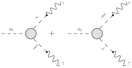
Figure 12: VMD diagrams for $a_{2}\to\gamma\gamma$.

This gives in analogy to the discussion above

$$a_{a_{2}\gamma\gamma}=2\frac{e^{2}}{\gamma_{\rho}\gamma_{\omega}}a_{a_{2}\omega\rho}\,,\qquad b_{a_{2}\gamma\gamma}=2\frac{e^{2}}{\gamma_{\rho}\gamma_{\omega}}b_{a_{2}\omega\rho}\,.$$ (7.37)

Here the coupling constants $a_{a_{2}\omega\rho}$ and $b_{a_{2}\omega\rho}$ are defined as in (3.41) for $a_{2}\gamma\gamma$ but with $\gamma\gamma$ replaced by $\omega\rho$. With the assumptions

$$a_{a_{2}\omega\rho}\approx a_{a_{2R}\omega\rho}\,,\qquad b_{a_{2}\omega\rho}\approx b_{a_{2R}\omega\rho}$$ (7.38)

we get from (7.37)

$$\begin{split}a_{a_{2R}\omega\rho}&=(2\alpha)^{-1}\bigg{(}\frac{4\pi}{\gamma_{\rho}^{2}}\frac{4\pi}{\gamma_{\omega}^{2}}\bigg{)}^{-1/2}a_{a_{2}\gamma\gamma}\,,\\ b_{a_{2R}\omega\rho}&=(2\alpha)^{-1}\bigg{(}\frac{4\pi}{\gamma_{\rho}^{2}}\frac{4\pi}{\gamma_{\omega}^{2}}\bigg{)}^{-1/2}b_{a_{2}\gamma\gamma}\,.\end{split}$$ (7.39)

In (5.38) we have obtained a number for the sum of the squared $a_{2}\gamma\gamma$ couplings. In order to estimate the couplings individually we shall make the ad hoc assumption that

$$m_{a_{2}}^{3}a_{a_{2}\gamma\gamma}=m_{f_{2}}^{3}a_{f_{2}\gamma\gamma}\cdot r\,,\qquad m_{a_{2}}b_{a_{2}\gamma\gamma}=m_{f_{2}}b_{f_{2}\gamma\gamma}\cdot r$$ (7.40)

with a real scale factor $r$. Then $r^{2}$ is given by the ratio of the r. h. sides of (5.38) and (5.30) and we get

$$r^{2}=\frac{3.60}{11.62}\,,\qquad r=\pm 0.56\,.$$ (7.41)

Here we must leave the sign of $r$ open. With the numbers for $a_{f_{2}\gamma\gamma}$ and $b_{f_{2}\gamma\gamma}$ from (3.40) we have now

$$a_{a_{2}\gamma\gamma}=\pm\frac{e^{2}}{4\pi}0.74~{}\text{GeV}^{-3}\,,\qquad b_{a_{2}\gamma\gamma}=\pm\frac{e^{2}}{4\pi}1.35~{}\text{GeV}^{-1}\,.$$ (7.42)

From (7.39), (7.42) and $\gamma^{2}_{\rho}/(4\pi)$, $\gamma^{2}_{\omega}/4\pi$ from (3.25) we get as estimates

$$a_{a_{2R}\omega\rho}=\pm 2.56~{}\text{GeV}^{-3}\,,\qquad b_{a_{2R}\omega\rho}=\pm 4.68~{}\text{GeV}^{-1}\,.$$ (7.43)

The numbers from (7.42) and (7.43) are taken as default values in (3.41) and (3.58), respectively. We emphasize that these should be considered as very rough estimates.

8 Conclusions

In this article we have proposed a model for soft high-energy reactions. The model is formulated in terms of effective propagators and vertices for the exchange objects: pomeron, odderon and reggeons. The vertices are constructed according to the standard rules of QFT and the effective propagators take into account the crossing properties of the amplitudes and the power laws, in the c. m. energy squared $s$, as suggested by the Regge ansatz. We have given the Feynman rules for our model in section 3 and someone only interested in applying the model for concrete calculations of amplitudes just has to read that section. The justification of the propagators and vertices of section 3 has been given in sections 4 to 7. In section 4 we have dealt with vector mesons and we have given an interpretation of the time-honoured vector-meson-dominance (VMD) model which we find quite satisfactory. We have shown how, starting from a perfectly gauge-invariant coupling of the photon to the vector mesons $V=\rho^{0},\omega,\phi$, one arrives at the standard VMD couplings; see section 4.2. In section 6.1 we have dealt with the pomeron. We have formulated pomeron exchange as an effective rank-two tensor exchange, that is, as spin 2 exchange. For the amplitudes of $pp$ and $\bar{p}p$ elastic scattering this leads at high energies to the same expressions as obtained from the Donnachie-Landshoff pomeron. We emphasise that applying the standard QFT rules to the exchange of our spin 2 pomeron automatically gives equality of the pomeron part of the $pp$ and $\bar{p}p$ elastic amplitudes. Furthermore, we have found it easy to write down QFT vertices for the coupling of our tensor pomeron to two vector particles. This is important for applications of our model to photon-induced reactions where the question of gauge invariance arises; see [19]. In section 6.2 we have discussed the odderon as an effective vector exchange. In section 6.3 we have presented our ansatz for reggeon exchanges. We consider the $f_{2}$ and $a_{2}$ reggeons as effective rank-two tensor exchanges and the $\rho$ and $\omega$ reggeons as effective vector exchanges.

We note that already many years ago attempts were made to understand the pomeron as a tensor; see [65, 66, 67]. In these papers typically it was tried to relate the properties of the pomeron to those of mesonic trajectories. But we believe now that the pomeron is predominantly a gluonic object. Thus, its properties are not – and should not be – directly related to those of the reggeons. Our present model for the pomeron takes this into account and is, therefore, completely different from the models of [65, 66, 67].

Our attempts to determine the parameters of our model as far as possible from data have been presented in sections 6.3, 7.1, and 7.2. We have, in particular, considered fits to total cross-section data as presented in [9]. In this way we have obtained default values for most of the parameters of our model. Clearly, it would be desirable to test the model in detail with a global fit to the available data. This is beyond the scope of the present work and must be left for future investigations. In this article we have restricted ourselves to the soft high-energy reactions listed in section 2. It is straightforward to extend the model to other reactions of this type, for instance, reactions involving kaons, $\phi$ mesons, and hyperons. Also central production of mesons in proton-proton collisions can be discussed,

$$p+p\longrightarrow p+\mathrm{meson}+p\,.$$ (8.1)

Such reactions are of particular interest since they have been studied experimentally and can be studied further in future experiments. A paper on central production based on our model is in preparation [68]. The model may also be applied to reactions suitable for odderon searches and to reactions involving polarised protons.

To summarise: the model for soft high-energy reactions which we have developed in this article has as main purpose a practical one. The model should allow easy calculations, using standard rules of QFT, for a variety of soft reactions. The hope is that it will provide a sort of standard against which experimentalists may compare their data in detail, that is, including all angular and spin distributions.

Appendix A The $f_{2}$ Propagator in Detail

Here we construct in detail our model for the $f_{2}$ propagator. Throughout this section we work in pure strong interaction dynamics neglecting electromagnetic effects. We start by constructing for given four-momentum $k$ with $k^{0}>0$ and $k^{2}>0$ the symmetric rank 2 polarisation tensors corresponding to spin 2, spin 1 and spin 0. For this we assume $\vec{k}\neq 0$, use the coordinate system (5.11) and define as in (5.12) but with $m_{f_{2}}$ replaced by $\sqrt{k^{2}}$

$$\epsilon^{(\pm)\mu}(k)=\mp\frac{1}{\sqrt{2}}\begin{pmatrix}0\\ \vec{e}_{1}\pm i\vec{e}_{2}\end{pmatrix}\,,\qquad\epsilon^{(0)\mu}(k)=\frac{1}{\sqrt{k^{2}}}\begin{pmatrix}|\vec{k}|\\ \vec{e}_{3}k^{0}\end{pmatrix}\,.$$ (A.1)

A basis for the polarisation tensors of spin 2, $\epsilon^{(m)\mu\nu}(k)$ with $m\in\{-2,\dots 2\}$, is defined as in (5.13), but with $\epsilon^{(m_{i})\mu}(k)$ from (A.1). A basis for spin 1 is given by

$$\eta^{(m)\mu\nu}(k)=\frac{1}{\sqrt{2k^{2}}}(k^{\mu}\epsilon^{(m)\nu}(k)+\epsilon^{(m)\mu}(k)k^{\nu})\,,\quad m\in\{1,0,-1\}\,.$$ (A.2)

We have two possibilities for spin $\mathrm{𝟎}$ polarisation tensors:

$$\begin{split}\xi^{(1)\mu\nu}(k)&=\frac{k^{\mu}k^{\nu}}{k^{2}}\,,\\ \xi^{(2)\mu\nu}(k)&=\frac{1}{\sqrt{3}}\left(-g^{\mu\nu}+\frac{k^{\mu}k^{\nu}}{k^{2}}\right)\,.\end{split}$$ (A.3)

The following relations are easily checked:

$$\left(\epsilon^{(m)\mu}(k)\right)^{*}\epsilon^{(n)}_{\mu}(k) =-\delta_{mn}\,,$$ (A.4)

$$\left(\epsilon^{(m)\mu\nu}(k)\right)^{*}\epsilon^{(n)}_{\mu\nu}(k) =\delta_{mn}\,,$$ (A.5)

$$\left(\epsilon^{(m)\mu\nu}(k)\right)^{*}\eta^{(n)}_{\mu\nu}(k) =0\,,$$ (A.6)

$$\left(\epsilon^{(m)\mu\nu}(k)\right)^{*}\xi^{(a)}_{\mu\nu}(k) =0\,,$$ (A.7)

$$\left(\eta^{(m)\mu\nu}(k)\right)^{*}\eta^{(n)}_{\mu\nu}(k) =-\delta_{mn}\,,$$ (A.8)

$$\left(\eta^{(m)\mu\nu}(k)\right)^{*}\xi^{(a)}_{\mu\nu}(k) =0\,,$$ (A.9)

$$\left(\xi^{(a)\mu\nu}(k)\right)^{*}\xi^{(b)}_{\mu\nu}(k) =\delta_{ab}\,.$$ (A.10)

Here it is understood that $m,n,a,b$ run over the appropriate index ranges.

Now we construct the tensors $P^{(i)}$ (5.17) by defining

$$\begin{split}P^{(2)}_{\mu\nu,\kappa\lambda}(k)=&\sum^{2}_{m=-2}\epsilon^{(m)}_{\mu\nu}(k)\left(\epsilon^{(m)}_{\kappa\lambda}(k)\right)^{*}\\ =&\,\frac{1}{2}\left(-g_{\mu\kappa}+\frac{k_{\mu}k_{\kappa}}{k^{2}}\right)\left(-g_{\nu\lambda}+\frac{k_{\nu}k_{\lambda}}{k^{2}}\right)+\frac{1}{2}\left(-g_{\mu\lambda}+\frac{k_{\mu}k_{\lambda}}{k^{2}}\right)\left(-g_{\nu\kappa}+\frac{k_{\nu}k_{\kappa}}{k^{2}}\right)\\ &-\frac{1}{3}\left(-g_{\mu\nu}+\frac{k_{\mu}k_{\nu}}{k^{2}}\right)\left(-g_{\kappa\lambda}+\frac{k_{\kappa}k_{\lambda}}{k^{2}}\right)\,,\end{split}$$ (A.11)

$$\begin{split}P^{(1)}_{\mu\nu,\kappa\lambda}(k)=&\sum^{1}_{m=-1}\eta^{(m)}_{\mu\nu}(k)\left(\eta^{(m)}_{\kappa\lambda}(k)\right)^{*}\\ =&\,\frac{1}{2k^{2}}\Bigg{\{}k_{\mu}k_{\kappa}\left(-g_{\nu\lambda}+\frac{k_{\nu}k_{\lambda}}{k^{2}}\right)+k_{\mu}k_{\lambda}\left(-g_{\nu\kappa}+\frac{k_{\nu}k_{\kappa}}{k^{2}}\right)\\ &\hskip 30.0pt+k_{\nu}k_{\kappa}\left(-g_{\mu\lambda}+\frac{k_{\mu}k_{\lambda}}{k^{2}}\right)+k_{\nu}k_{\lambda}\left(-g_{\mu\kappa}+\frac{k_{\mu}k_{\kappa}}{k^{2}}\right)\Bigg{\}}\,,\end{split}$$ (A.12)

$$P^{(0,ab)}_{\mu\nu,\kappa\lambda}(k)=\xi^{(a)}_{\mu\nu}(k)\left(\xi^{(b)}_{\kappa\lambda}(k)\right)^{*}\,,$$ (A.13)

$$P^{(0,11)}_{\mu\nu,\kappa\lambda}(k)=\frac{k_{\mu}k_{\nu}}{k^{2}}\frac{k_{\kappa}k_{\lambda}}{k^{2}}\,,$$ (A.14)

$$P^{(0,22)}_{\mu\nu,\kappa\lambda}(k)=\frac{1}{3}\left(-g_{\mu\nu}+\frac{k_{\mu}k_{\nu}}{k^{2}}\right)\left(-g_{\kappa\lambda}+\frac{k_{\kappa}k_{\lambda}}{k^{2}}\right)\,,$$ (A.15)

$$P^{(0,12)}_{\mu\nu,\kappa\lambda}(k)=\frac{k_{\mu}k_{\nu}}{k^{2}}\frac{1}{\sqrt{3}}\left(-g_{\kappa\lambda}+\frac{k_{\kappa}k_{\lambda}}{k^{2}}\right)\,,$$ (A.16)

$$P^{(0,21)}_{\mu\nu,\kappa\lambda}(k)=\frac{1}{\sqrt{3}}\left(-g_{\mu\nu}+\frac{k_{\mu}k_{\nu}}{k^{2}}\right)\frac{k_{\kappa}k_{\lambda}}{k^{2}}\,.$$ (A.17)

We have the following relations

$$\begin{split}P^{(2)}(k)P^{(2)}(k)&=P^{(2)}(k)\,,\\ P^{(2)}(k)P^{(1)}(k)&=0\,,\\ P^{(2)}(k)P^{(0,ab)}(k)&=0\,,\\ P^{(1)}(k)P^{(1)}(k)&=-P^{(1)}(k)\,,\\ P^{(1)}(k)P^{(0,ab)}(k)&=0\,,\\ P^{(0,ab)}(k)P^{(0,cd)}(k)&=\delta_{bc}P^{(0,ad)}(k)\,.\end{split}$$ (A.18)

Here we use matrix notation. That is, the first eq. of (A.18) reads in detail

$$P^{(2)}_{\mu\nu,\rho\sigma}(k)P^{(2)\rho\sigma}{}_{\kappa\lambda}(k)=P^{(2)}_{\mu\nu,\kappa\lambda}(k)\,,$$ (A.19)

etc. Furthermore, we get the trace relations

$$\begin{split}P^{(2)}_{\mu\nu}{}^{\mu\nu}(k)&=5\,,\\ P^{(1)}_{\mu\nu}{}^{\mu\nu}(k)&=-3\,,\\ P^{(0,ab)}_{\mu\nu}{}^{\mu\nu}(k)&=\delta_{ab}\,,\end{split}$$ (A.20)

and the completeness relation

$$\left(P^{(2)}(k)-P^{(1)}(k)+P^{(0,11)}(k)+P^{(0,22)}(k)\right)_{\mu\nu,\kappa\lambda}=\frac{1}{2}(g_{\mu\kappa}g_{\nu\lambda}+g_{\mu\lambda}g_{\nu\kappa})\,.$$ (A.21)

Now we come to the general tensor-field propagator (5.10). With the help of the $P^{(i)}$, (A.11) to (A.17), we can write down the expansion (5.17) where $\Delta^{(2)}(k^{2})$, $\Delta^{(1)}(k^{2})$, and $\Delta^{(0)}_{ab}(k^{2})$ are invariant functions. For the free propagator (5.16) these read

$$\begin{split}\left.\Delta^{(2)}(k^{2})\right|_{\rm free}&=\frac{1}{k^{2}-m^{2}_{f_{2}}+i\epsilon}\,,\\ \left.\Delta^{(1)}(k^{2})\right|_{\rm free}&=\frac{1}{m^{2}_{f_{2}}}\,,\\ \left.\Delta^{(0)}_{11}(k^{2})\right|_{\rm free}&=\frac{2}{3}\frac{k^{2}-m^{2}_{f_{2}}}{(m_{f_{2}})^{4}}\,,\\ \left.\Delta^{(0)}_{12}(k^{2})\right|_{\rm free}=\left.\Delta^{(0)}_{21}(k^{2})\right|_{\rm free}&=-\frac{1}{\sqrt{3}}\frac{1}{m^{2}_{f_{2}}}\,,\\ \left.\Delta^{(0)}_{22}(k^{2})\right|_{\rm free}&=0\,.\end{split}$$ (A.22)

We analyze now the full tensor-field propagator (5.17) in the same spirit as done for the $\gamma$-$\rho$-$\omega$ system in [22]. From (5.10) we get

$$\Delta^{(T)}_{\mu\nu,\kappa\lambda}(k)-\big{(}\Delta^{(T)}_{\kappa\lambda,\mu\nu}(k)\big{)}^{*}=\frac{1}{i}\int d^{4}x\,e^{ikx}\langle 0|\big{\{}\phi_{\mu\nu}(x)\phi_{\kappa\lambda}(0)+\phi_{\kappa\lambda}(0)\phi_{\mu\nu}(x)\big{\}}|0\rangle\,.$$ (A.23)

Inserting a complete set of intermediate states we get for $k^{0}>0$

$$\Delta^{(T)}_{\mu\nu,\kappa\lambda}(k)-\big{(}\Delta^{(T)}_{\kappa\lambda,\mu\nu}(k)\big{)}^{*}=\frac{1}{i}\sum_{X}(2\pi)^{4}\delta^{(4)}(k-p_{X})\langle 0|\phi_{\mu\nu}(0)|X(p_{X})\rangle\langle X(p_{X})|\phi_{\kappa\lambda}(0)|0\rangle.$$ (A.24)

For the following we need the inverse propagator which in matrix notation is found to be

$$\big{(}\Delta^{(T)}\big{)}^{-1}(k)=P^{(2)}(k)\big{(}\Delta^{(2)}(k^{2})\big{)}^{-1}+P^{(1)}(k)\big{(}\Delta^{(1)}(k^{2})\big{)}^{-1}+P^{(0,ab)}(k)\big{(}\big{(}\Delta^{(0)}\big{)}^{-1}(k^{2})\big{)}_{ab}\,.$$ (A.25)

As done in [22] for the vector propagators we define now reduced matrix elements by

$$\begin{split}&\langle X(p_{X})\|\phi_{\mu\nu}\|0\rangle=\langle X(p_{X})|\phi^{\kappa\lambda}(0)|0\rangle\big{(}\big{(}\Delta^{(T)}\big{)}^{-1}(p_{X})\big{)}_{\kappa\lambda,\mu\nu}\,,\\ &\langle 0\|\phi_{\mu\nu}\|X(p_{X})\rangle=\langle X(p_{X})\|\phi_{\mu\nu}\|0\rangle^{*}\,.\end{split}$$ (A.26)

We get from (A.24) and (A.25), always for $k^{0}>0$,

$$\begin{split}\frac{1}{2i}\big{[}\big{(}\Delta^{(T)}\big{)}^{-1}(k)-\big{(}\big{(}\Delta^{(T)}\big{)}^{-1}(k)\big{)}^{\dagger}\big{]}_{\mu\nu,\kappa\lambda}=&\frac{1}{2}\sum_{X}(2\pi)^{4}\delta^{(4)}(k-p_{X})\\ &\times\langle 0\|\phi_{\mu\nu}\|X(p_{X})\rangle\langle X(p_{X})\|\phi_{\kappa\lambda}\|0\rangle\,.\end{split}$$ (A.27)

Contracting with $P^{(2)}(k)$ gives

$$\begin{split}&\frac{1}{2i}\left[(\Delta^{(2)}(k^{2}))^{-1}-((\Delta^{(2)}(k^{2}))^{-1})^{*}\right]\\ &=\frac{1}{2}\sum_{X}(2\pi)^{4}\delta^{(4)}(k-p_{X})\,\frac{1}{5}\!\sum^{2}_{m=-2}(\epsilon^{(m)\mu\nu}(k))^{*}\langle 0\|\phi_{\mu\nu}\|X(p_{X})\rangle\langle X(p_{X})\|\phi_{\kappa\lambda}\|0\rangle\epsilon^{(m)\kappa\lambda}(k)\,.\end{split}$$ (A.28)

As already discussed in section 5, the function $\Delta^{(2)}(k^{2})$ is the one where the $f_{2}$ resonance appears. We shall define the squared $f_{2}$ mass as zero point of the real part of the inverse of $\Delta^{(2)}$:

$$\text{Re}\,\big{(}\Delta^{(2)}(m^{2}_{f_{2}})\big{)}^{-1}=0\,.$$ (A.29)

Then we will normalise the tensor field $\phi_{\mu\nu}$ such that

$$\big{(}\Delta^{(2)}(0)\big{)}^{-1}=-m^{2}_{f_{2}}$$ (A.30)

and define $B_{f_{2}}(k^{2})$ by

$$\big{(}\Delta^{(2)}(k^{2})\big{)}^{-1}=-m^{2}_{f_{2}}+k^{2}+B_{f_{2}}(k^{2})\,.$$ (A.31)

With (A.29) and (A.30) we must require

$$B_{f_{2}}(0)=0\,,\quad\quad\text{Re}\,B_{f_{2}}(m^{2}_{f_{2}})=0\,.$$ (A.32)

From (A.28) we get, setting $s=k^{2}$,

$$\begin{split}\mathrm{Im}\,B_{f_{2}}(s)=&\,\frac{1}{2}\sum_{X}(2\pi)^{4}\delta^{(4)}(k-p_{X})\,\frac{1}{5}\sum^{2}_{m=-2}\big{(}\epsilon^{(m)\mu\nu}(k)\big{)}^{*}\langle 0\|\phi_{\mu\nu}\|X(p_{X})\rangle\\ &\times\langle X(p_{X})\|\phi_{\kappa\lambda}\|0\rangle\,\epsilon^{(m)\kappa\lambda}(k)\,.\end{split}$$ (A.33)

For an ‘on-shell’ $f_{2}$ we have

$$\langle X(k)|{\cal T}|f_{2}(k,\epsilon^{(m)}\big{)}\rangle=-\langle X(k)\|\phi_{\mu\nu}\|0\rangle\,\epsilon^{(m)\mu\nu}(k)\,,$$ (A.34)

as is easily seen from the reduction formula, and

$$\mathrm{Im}\,B_{f_{2}}(m^{2}_{f_{2}})=m_{f_{2}}\Gamma_{f_{2}}\,.$$ (A.35)

We assume now that $B_{f_{2}}(s)$ satisfies a once subtracted dispersion relation:

$$B_{f_{2}}(s)=B_{f_{2}}(0)+sB_{f_{2}}^{\prime}(0)+\frac{s^{2}}{\pi}\int^{\infty}_{4m^{2}_{\pi}}ds^{\prime}\frac{\mathrm{Im}\,B_{f_{2}}(s^{\prime})}{(s^{\prime})^{2}(s^{\prime}-s-i\epsilon)}\,.$$ (A.36)

In pure strong interactions the lowest intermediate states $|X\rangle$ in (A.33) are the two-pion states and, therefore, the dispersion integral in (A.36) starts at $s^{\prime}=4m^{2}_{\pi}$. We set now

$$R_{f_{2}}(s)=\frac{s}{\pi}\,\mbox{V.\,P.}\int^{\infty}_{4m^{2}_{\pi}}ds^{\prime}\frac{\mathrm{Im}\,B_{f_{2}}(s^{\prime})}{(s^{\prime})^{2}(s^{\prime}-s)}$$ (A.37)

where V. P. means the principal value prescription. The expressions for $B_{f_{2}}(s)$ and $(\Delta^{(2)}(s))^{-1}$ satisfying all the constraints (A.29), (A.30) and (A.32) read then

$$B_{f_{2}}(s)=s\big{[}R_{f_{2}}(s)-R_{f_{2}}(m^{2}_{f_{2}})\big{]}+i\,\mathrm{Im}\,B_{f_{2}}(s)\,,$$ (A.38)

$$\big{(}\Delta^{(2)}(s)\big{)}^{-1}=-m^{2}_{f_{2}}+s+s\big{[}R_{f_{2}}(s)-R_{f_{2}}(m^{2}_{f_{2}})\big{]}+i\,\mathrm{Im}\,B_{f_{2}}(s)\,.$$ (A.39)

It remains to construct $\mathrm{Im}\,B_{f_{2}}(s)$ explicitly. For the $\pi\pi$ intermediate states in (A.33) we get from (3.37)

$$\left.\mathrm{Im}\,B_{f_{2}}(s)\right|_{\pi\pi}=\frac{1}{320\pi}\left|\frac{g_{f_{2}\pi\pi}F^{(f_{2}\pi\pi)}(s)}{M_{0}}\right|^{2}s^{2}\left[1-\frac{4m^{2}_{\pi}}{s}\right]^{5/2}\theta(s-4m^{2}_{\pi})\,,$$ (A.40)

$$\begin{split}\mathrm{Im}\,B_{f_{2}}(s)|_{\pi^{+}\pi^{-}}&=\frac{2}{3}\,\mathrm{Im}\,B_{f_{2}}(s)|_{\pi\pi}\,,\\ \mathrm{Im}\,B_{f_{2}}(s)|_{\pi^{0}\pi^{0}}&=\frac{1}{3}\,\mathrm{Im}\,B_{f_{2}}(s)|_{\pi\pi}\,.\end{split}$$ (A.41)

Since the branching ratio $\Gamma(f_{2}\to\pi\pi)/\Gamma_{f_{2}}\cong 0.85$, see (5.7), we set as an approximation

$$\mathrm{Im}\,B_{f_{2}}(s)=\frac{\Gamma_{f_{2}}}{\Gamma(f_{2}\to\pi\pi)}\,\mathrm{Im}\,B_{f_{2}}(s)|_{\pi\pi}\,.$$ (A.42)

Inserting this in (A.37) to (A.39) leads to the $f_{2}$ propagator given in (5.19) to (5.22).

Finally, we consider $\pi^{+}\pi^{-}$ elastic scattering with exchange of an $f_{2}$ meson in the $s$ channel, see figure 13,

$$\pi^{+}(q_{1})+\pi^{-}(q_{2})\longrightarrow\pi^{+}(k_{1})+\pi^{-}(k_{2})\,,\qquad k=q_{1}+q_{2}=k_{1}+k_{2}\,.$$ (A.43)

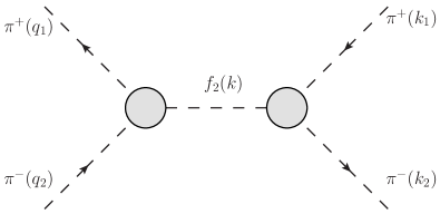
Figure 13: Scattering $\pi^{+}\pi^{-}\to\pi^{+}\pi^{-}$ with exchange of $f_{2}$ in the $s$ channel.

With the vertex (3.37) and the invariant function $\Delta^{(2)}(k^{2})$ from (5.19) we obtain for the T-matrix element in the c. m. system of the reaction (A.43)

$$\langle\pi^{+}(\vec{k}_{1}),\pi^{-}(-\vec{k}_{1})|\mathcal{T}|\pi^{+}(\vec{q}_{1}),\pi^{-}(-\vec{q}_{1})\rangle=16\pi\left(1-\frac{4m^{2}_{\pi}}{s}\right)^{-1/2}5a_{2}(s)P_{2}(\cos\vartheta)\,.$$ (A.44)

Here $\vartheta$ is the scattering angle,

$$\cos\vartheta=\frac{{\vec{k}}_{1}\cdot{\vec{q}}_{1}}{|{\vec{k}}_{1}||{\vec{q}}_{1}|}\,,$$ (A.45)

$P_{2}$ is the Legendre polynomial and

$$a_{2}(s)=-\mathrm{Im}\,B_{f_{2}}(s)|_{\pi^{+}\pi^{-}}\,\Delta^{(2)}(s)\,.$$ (A.46)

As it should be for $f_{2}$ exchange, scattering is only for orbital angular momentum $l=2$, $a_{2}(s)$ is the $l=2$ partial-wave amplitude, and the partial-wave unitary relation is respected. Indeed, with $\delta_{2}(s)$ the phase shift and $\eta_{2}(s)$ the inelasticity parameter we find from (A.46)

$$\begin{split}\eta_{2}(s)&e^{2i\delta_{2}(s)}=\,2ia_{2}(s)+1\\ =&\,\Big{\{}s-m^{2}_{f_{2}}+s\big{[}R_{f_{2}}(s)-R_{f_{2}}(m^{2}_{f_{2}})\big{]}-i\big{[}\mathrm{Im}\,B_{f_{2}}(s)|_{\pi^{+}\pi^{-}}-\mathrm{Im}\,\tilde{B}_{f_{2}}(s)\big{]}\Big{\}}\\ &\times\Big{\{}s-m^{2}_{f_{2}}+s\big{[}R_{f_{2}}(s)-R_{f_{2}}(m^{2}_{f_{2}})\big{]}+i\big{[}\mathrm{Im}\,B_{f_{2}}(s)|_{\pi^{+}\pi^{-}}+\mathrm{Im}\,\tilde{B}_{f_{2}}(s)\big{]}\Big{\}}^{-1}\,.\end{split}$$ (A.47)

Here we set

$$\mathrm{Im}\,\tilde{B}_{f_{2}}(s)=\mathrm{Im}\,B_{f_{2}}(s)-\mathrm{Im}\,B_{f_{2}}(s)|_{\pi^{+}\pi^{-}}\,,$$ (A.48)

that is, $\mathrm{Im}\,\tilde{B}_{f_{2}}(s)$ is defined as in (A.33) but with the sum over intermediate states $|X\rangle$ excluding the $\pi^{+}\pi^{-}$ states. Clearly we still have

$$\mathrm{Im}\,\tilde{B}_{f_{2}}(s)\geq 0\,.$$ (A.49)

For instance, with our approximation (A.42) we get

$$\mathrm{Im}\,\tilde{B}_{f_{2}}(s)=\left(\frac{\Gamma_{f_{2}}}{\Gamma(f_{2}\to\pi\pi)}-\frac{2}{3}\right)\mathrm{Im}\,B_{f_{2}}(s)|_{\pi\pi}>0\,.$$ (A.50)

From (A.47) and (A.49) we find

$$\left|\eta_{2}(s)\right|\leq 1$$ (A.51)

as it should be.

To conclude this section we note that our model for the $f_{2}$ propagator could easily be improved by also modelling the amplitudes for the states $|X\rangle\neq|\pi\pi\rangle$ in (A.33). These would be in first instance the four-pion and the $K\bar{K}$ states. We estimate that our $f_{2}$ propagator (5.19) to (5.22) should be a reasonable model for, say, $0<s<10\,\mbox{GeV}^{2}$. For larger $s$ we expect that further multi-particle states $|X\rangle$ in the sum (A.33) will become important. It may then be more reasonable to consider quark-antiquark states as final states $|X\rangle$ in (A.33). But this is beyond the scope of the present article.

Appendix B The Pomeron as Coherent Sum of Exchanges with Spin 2, 4, 6, etc

Here we show how to write the pomeron exchange amplitude for $pp$ scattering (6.1) as coherent sum of exchanges with spin $2$, $4$, $6$, etc. The technique is similar to the one used in section 6.2 of [51]. We start from (6.9) and (6.19) which give for the pomeron part of the $pp$ scattering amplitude for large $\nu$

$$\begin{split}\langle p(p^{\prime}_{1}),p(p^{\prime}_{2})|{\cal T}|p(p_{1}),p(p_{2})\rangle|_{\mathbbm{P}}\equiv&\,{\cal T}^{\mathbbm{P}}_{fi}=T^{(pp){\mathbbm{P}}}(\nu,t)\bar{u}(p^{\prime}_{1})\gamma^{\mu}u(p_{1})\bar{u}(p^{\prime}_{2})\gamma_{\mu}u(p_{2})\\ =&\,f(t)\exp\left[-i\pi\frac{1}{2}\big{(}\alpha_{\mathbbm{P}}(t)-2\big{)}\right](4\alpha^{\prime 2}_{\mathbbm{P}}\nu^{2})^{\frac{1}{2}(\alpha_{\mathbbm{P}}(t)-2)}2\alpha^{\prime}_{\mathbbm{P}}\nu\\ &\times\bar{u}(p^{\prime}_{1})\gamma^{\mu}u(p_{1})\bar{u}(p^{\prime}_{2})\gamma_{\mu}u(p_{2})\,.\end{split}$$ (B.1)

In the following we represent $\nu$ as

$$\nu=\frac{1}{4}(p_{1}+p^{\prime}_{1})\cdot(p_{2}+p^{\prime}_{2})\,.$$ (B.2)

Now we use the identity

$$(4\alpha^{\prime 2}_{\mathbbm{P}}\nu^{2})^{\frac{1}{2}(\alpha_{\mathbbm{P}}(t)-2)}=\frac{1}{\Gamma\left(1-\frac{1}{2}\alpha_{\mathbbm{P}}(t)\right)}\int^{\infty}_{0}d\tau\,\tau^{-\frac{1}{2}\alpha_{\mathbbm{P}}(t)}\exp(-4\alpha^{\prime 2}_{\mathbbm{P}}\nu^{2}\tau)\,.$$ (B.3)

Inserting (B.3) in (B.1) we get

$${\cal T}^{\mathbbm{P}}_{fi}=\tilde{f}(t)\int^{\infty}_{0}d\tau\,\tau^{-\frac{1}{2}\alpha_{\mathbbm{P}}(t)}\exp(-4\alpha^{\prime 2}_{\mathbbm{P}}\nu^{2}\tau)\,2\alpha^{\prime}_{\mathbbm{P}}\nu\,\bar{u}(p^{\prime}_{1})\gamma^{\mu}u(p_{1})\bar{u}(p^{\prime}_{2})\gamma_{\mu}u(p_{2})$$ (B.4)

where

$$\tilde{f}(t)=f(t)\exp\left[-i\pi\frac{1}{2}(\alpha_{\mathbbm{P}}(t)-2)\right]\Gamma^{-1}\left(1-\frac{1}{2}\alpha_{\mathbbm{P}}(t)\right).$$ (B.5)

Expanding the exponential function in (B.4) we find

$${\cal T}^{\mathbbm{P}}_{f_{i}}=\tilde{f}(t)\int^{\infty}_{0}d\tau\,\tau^{-\frac{1}{2}\alpha_{\mathbbm{P}}(t)}\sum^{\infty}_{n=1}\frac{(-\tau)^{(n-1)}}{(n-1)!}(2\alpha^{\prime}_{\mathbbm{P}}\nu)^{2n-1}\,\bar{u}(p^{\prime}_{1})\gamma^{\mu}u(p_{1})\bar{u}(p^{\prime}_{2})\gamma_{\mu}u(p_{2})\,.$$ (B.6)

For large $\nu$ we have, using (6.24) and (B.2)

$$\begin{split}(2\alpha^{\prime}_{\mathbbm{P}}\nu)^{2n-1}\,\bar{u}(p^{\prime}_{1})\gamma^{\mu}u(p_{1})\bar{u}(p^{\prime}_{2})\gamma_{\mu}u(p_{2})=&\left(\frac{1}{2}\alpha^{\prime}_{\mathbbm{P}}\right)^{2n-1}\bar{u}(p^{\prime}_{1})R^{\mu_{1}\dots\mu_{2n}}(p^{\prime}_{1},p_{1})u(p_{1})\\ &\times\bar{u}(p^{\prime}_{2})R_{\mu_{1}\dots\mu_{2n}}(p^{\prime}_{2},p_{2})u(p_{2})\end{split}$$ (B.7)

where

$$\begin{split}R^{\mu_{1}\dots\mu_{2n}}(p^{\prime},p)=&\,\frac{1}{2n}\big{\{}\gamma^{\mu_{1}}(p^{\prime}+p)^{\mu_{2}}\dots(p^{\prime}+p)^{\mu_{2n}}+(p^{\prime}+p)^{\mu_{1}}\gamma^{\mu_{2}}\dots(p^{\prime}+p)^{\mu_{2n}}\\ &\,+\dots+(p^{\prime}+p)^{\mu_{1}}\dots(p^{\prime}+p)^{\mu_{2n-1}}\gamma^{\mu_{2n}}\big{\}}\,.\end{split}$$ (B.8)

Inserting (B.8) in (B.7) we can write ${\cal T}_{fi}^{\mathbbm{P}}$ as coherent sum of exchanges with spin $2$, $4$, $6$, …,

$$\begin{split}{\cal T}^{\mathbbm{P}}_{fi}=&\,\tilde{f}(t)\int^{\infty}_{0}d\tau\,\tau^{-\frac{1}{2}\alpha_{\mathbbm{P}}(t)}\sum^{\infty}_{n=1}\frac{(-\tau)^{n-1}}{(n-1)!}\left(\frac{1}{2}\alpha^{\prime}_{\mathbbm{P}}\right)^{2n-1}\\ &\times\bar{u}(p^{\prime}_{1})R^{\mu_{1}\dots\mu_{2n}}(p^{\prime}_{1},p_{1})u(p_{1})\bar{u}(p^{\prime}_{2})R_{\mu_{1}\dots\mu_{2n}}(p^{\prime}_{2},p_{2})u(p_{2})\,.\end{split}$$ (B.9)

Note that the infinite sum in (B.9) starts with spin $2$ and not with spin $\mathrm{𝟎}$ exchange. For spin $\mathrm{𝟎}$ exchange we would have to have a structure

$${\cal T}^{\mathbbm{P}}_{fi}\propto\bar{u}(p^{\prime}_{1})u(p_{1})\bar{u}(p^{\prime}_{2})u(p_{2})\,.$$ (B.10)

For high-energy small-angle scattering this would give $s$-channel-helicity-conserving, single- and double-helicity-flip amplitudes of the same order of magnitude. This is not what is seen by experiment which finds predominantly $s$-channel-helicity conservation; for recent $pp$ experimental results see for instance [69, 70]. As is well known, one can understand this from QCD where gluons couple in a chirality conserving way to quarks. For high energy quark-quark scattering this leads to quark-helicity conservation, as can be seen, for instance, from the general analysis of this process in [51]. There and in [54] it is shown – in a model – how this leads also to helicity conservation for hadron-hadron scattering.

Finally we remark that the odderon-exchange amplitude (6.2), (6.2) can be understood as arising from the coherent sum of spin 1, 3, 5, …exchanges. This can easily be shown with the help of the above techniques.

References

- [1] D. J. Gross and F. Wilczek, Phys. Rev. Lett. 30 (1973) 1343.
- [2] H. D. Politzer, Phys. Rev. Lett. 30 (1973) 1346.
- [3] K. G. Wilson, Phys. Rev. D 10 (1974) 2445.
- [4] T. Regge, Nuovo Cim. 14 (1959) 951.
- [5] G. F. Chew and S. C. Frautschi, Phys. Rev. Lett. 8 (1962) 41.
- [6] V. N. Gribov, Y. L. Dokshitzer and J. Nyiri, Strong Interactions of Hadrons at High Energies: Gribov Lectures on Theoretical Physics, Cambridge University Press, 2009
- [7] P. D. B. Collins, An Introduction to Regge Theory and High-Energy Physics, Cambridge University Press, 1977
- [8] P. D. B. Collins and A. D. Martin, Hadron Interactions, Adam Hilger, Bristol 1984
- [9] A. Donnachie, H. G. Dosch, P. V. Landshoff and O. Nachtmann, Pomeron physics and QCD, Camb. Monogr. Part. Phys. Nucl. Phys. Cosmol. 19 (2002) 1.
- [10] L. Caneschi (ed.), Regge Theory of Low- Hadronic Interactions, Elsevier Science Publishers B. V., Amsterdam 1989
- [11] M. Haguenauer, B. Nicolescu, and J. Tran Thanh Van (eds.), Proc. XIth International Conference on Elastic and Diffractive Scattering, Towards High Energy Frontiers, Thê Giôi Publishers, Vietnam, 2006
- [12] L. Lukaszuk and B. Nicolescu, Lett. Nuovo Cim. 8 (1973) 405.
- [13] D. Joynson, E. Leader, B. Nicolescu and C. Lopez, Nuovo Cim. A 30 (1975) 345.
- [14] C. Ewerz, The Odderon in Quantum Chromodynamics, hep-ph/0306137.
- [15] P. V. Landshoff and J. C. Polkinghorne, Nucl. Phys. B 32 (1971) 541.
- [16] A. Donnachie and P. V. Landshoff, Nucl. Phys. B 231 (1984) 189.
- [17] A. Donnachie and P. V. Landshoff, Nucl. Phys. B 267 (1986) 690.
- [18] A. Donnachie and P. V. Landshoff, Nucl. Phys. B 303 (1988) 634.
- [19] C. Ewerz, M. Maniatis, O. Nachtmann, M. Sauter, A. Schöning, in preparation
- [20] J. Beringer et al. [Particle Data Group Collaboration], Phys. Rev. D 86 (2012) 010001.
- [21] O. Nachtmann, Elementary Particle Physics: Concepts and Phenomena, Springer Verlag, Berlin, 1990
- [22] D. Melikhov, O. Nachtmann, V. Nikonov and T. Paulus, Eur. Phys. J. C 34 (2004) 345 [hep-ph/0311213].
- [23] F. E. Close, (ed.), A. Donnachie, (ed.) and G. Shaw, (ed.), Electromagnetic interactions and hadronic structure, Cambridge monographs on particle physics, nuclear physics and cosmology 25 (2007) 1
- [24] M. H. Johnson and E. Teller, Phys. Rev. 98 (1955) 783.
- [25] H.-P. Duerr and E. Teller, Phys. Rev. 101 (1956) 494.
- [26] H.-P. Duerr, Phys. Rev. 103 (1956) 469.
- [27] Y. Nambu, Phys. Rev. 106 (1957) 1366.
- [28] W. R. Frazer and J. R. Fulco, Phys. Rev. Lett. 2 (1959) 365.
- [29] W. R. Frazer and J. R. Fulco, Phys. Rev. 117 (1960) 1609.
- [30] J. J. Sakurai, Annals Phys. 11 (1960) 1.
- [31] M. Gell-Mann and F. Zachariasen, Phys. Rev. 124 (1961) 953.
- [32] T. H. Bauer, R. D. Spital, D. R. Yennie and F. M. Pipkin, Rev. Mod. Phys. 50 (1978) 261 [Erratum-ibid. 51 (1979) 407].
- [33] D. Schildknecht, Acta Phys. Polon. B 37 (2006) 595 [hep-ph/0511090].
- [34] D. H. Sharp and W. G. Wagner, Phys. Rev. 131 (1963) 2226.
- [35] S. Weinberg, Phys. Rev. 133 (1964) B1318.
- [36] S.-J. Chang, Phys. Rev. 148 (1966) 1259.
- [37] S. Bellucci, J. Gasser and M. E. Sainio, Nucl. Phys. B 423 (1994) 80 [Erratum-ibid. B 431 (1994) 413] [hep-ph/9401206].
- [38] D. Toublan, Phys. Rev. D 53 (1996) 6602 [Erratum-ibid. D 57 (1998) 4495] [hep-ph/9509217].
- [39] Y. Oh and T.-S. H. Lee, Phys. Rev. C 69 (2004) 025201 [nucl-th/0306033].
- [40] M. R. Pennington, T. Mori, S. Uehara and Y. Watanabe, Eur. Phys. J. C 56 (2008) 1 [arXiv:0803.3389 [hep-ph]].
- [41] J. D. Bjorken and S. D. Drell, Relativistic quantum fields, McGraw Hill, 1965.
- [42] F. E. Low, Phys. Rev. D 12 (1975) 163.
- [43] S. Nussinov, Phys. Rev. Lett. 34 (1975) 1286.
- [44] J. F. Gunion and D. E. Soper, Phys. Rev. D 15 (1977) 2617.
- [45] E. A. Kuraev, L. N. Lipatov and V. S. Fadin, Sov. Phys. JETP 45 (1977) 199 [Zh. Eksp. Teor. Fiz. 72 (1977) 377].
- [46] I. I. Balitsky and L. N. Lipatov, Sov. J. Nucl. Phys. 28 (1978) 822 [Yad. Fiz. 28 (1978) 1597].
- [47] L. N. Lipatov, Phys. Rept. 286 (1997) 131 [arXiv:hep-ph/9610276].
- [48] V. S. Fadin and L. N. Lipatov, Phys. Lett. B 429 (1998) 127 [hep-ph/9802290].
- [49] M. Ciafaloni and G. Camici, Phys. Lett. B 430 (1998) 349 [hep-ph/9803389].
- [50] P. V. Landshoff and O. Nachtmann, Z. Phys. C 35 (1987) 405.
- [51] O. Nachtmann, Annals Phys. 209 (1991) 436.
- [52] H. G. Dosch, E. Ferreira and A. Krämer, Phys. Lett. B 289 (1992) 153.
- [53] H. G. Dosch, E. Ferreira and A. Krämer, Phys. Rev. D 50 (1994) 1992 [hep-ph/9405237].
- [54] O. Nachtmann, High-energy collisions and nonperturbative QCD, in Proceedings of 35. Internationale Universitätswochen für Kern- und Teilchenphysik, Schladmig, Austria, 1996, H. Latal, W. Schweiger (Eds.) Springer Verlag, Berlin, Heidelberg 1997 [hep-ph/9609365].
- [55] E. R. Berger and O. Nachtmann, Eur. Phys. J. C 7 (1999) 459 [hep-ph/9808320].
- [56] A. I. Shoshi, F. D. Steffen and H. J. Pirner, Nucl. Phys. A 709 (2002) 131 [hep-ph/0202012].
- [57] E. Meggiolaro, Z. Phys. C 76 (1997) 523 [hep-th/9602104].
- [58] E. Meggiolaro, Phys. Lett. B 651 (2007) 177 [hep-ph/0612307].
- [59] M. Giordano and E. Meggiolaro, Phys. Rev. D 78 (2008) 074510 [arXiv:0808.1022 [hep-lat]].
- [60] R. Fiore, L. L. Jenkovszky, R. Orava, E. Predazzi, A. Prokudin and O. Selyugin, Int. J. Mod. Phys. A 24 (2009) 2551 [arXiv:0810.2902 [hep-ph]].
- [61] P. Lebiedowicz and A. Szczurek, Phys. Rev. D 81 (2010) 036003 [arXiv:0912.0190 [hep-ph]].
- [62] G. Antchev et al. [TOTEM Collaboration], Europhys. Lett. 101 (2013) 21002.
- [63] A. Donnachie and P. V. Landshoff, and total cross sections and elastic scattering,” arXiv:1309.1292 [hep-ph].
- [64] Durham HepData Database, http://durpdg.dur.ac.uk/hepdata/
- [65] P. G. O. Freund, Phys. Lett. 2 (1962), 136
- [66] P. G. O. Freund, Nuovo Cim. A 5 (1971) 9.
- [67] R. D. Carlitz, M. B. Green and A. Zee, Phys. Rev. Lett. 26 (1971) 1515.
- [68] P. Lebiedowicz, O. Nachtmann and A. Szczurek, in preparation
- [69] L. Adamczyk et al. [STAR Collaboration], Phys. Lett. B 719 (2013) 62 [arXiv:1206.1928 [nucl-ex]].
- [70] A. Sandacz, talk at the workshop ”Exclusive and diffractive processes in high energy proton-proton and nucleus-nucleus collisions”, ECT∗ Trento, Feb. 27 - Mar. 2, 2012