Scaling quasi-stationary states in long range systems with dissipation

Abstract

Hamiltonian systems with long-range interactions give rise to long lived out of equilibrium macroscopic states, so-called quasi-stationary states. We show here that, in a suitably generalized form, this result remains valid for many such systems in the presence of dissipation. Using an appropriate mean-field kinetic description, we show that models with dissipation due to a viscous damping or due to inelastic collisions admit “scaling quasi-stationary states”, i.e., states which are quasi-stationary in rescaled variables. A numerical study of one dimensional self-gravitating systems confirms both the relevance of these solutions, and gives indications of their regime of validity in line with theoretical predictions. We underline that the velocity distributions never show any tendency to evolve towards a Maxwell-Boltzmann form.

Physical systems characterized by long range interactions (for reviews, see e.g. Campa2009 ; Bouchet2010 ) are ubiquitous, encompassing systems as diverse as self-gravitating bodies in astrophysics, plasmas PhysRevLett.100.040604 , lasers Antoniazzietal_2006 , cold atoms Chalony2013 in the laboratory, and even biological systems sopiketal_2005 . One of the main results of recent years about such systems is that, quite generically, they relax, on times scales characterized by the mean force field, towards long-lived macroscopic states called quasi-stationary states (QSS) [e.g. galaxies in astrophysics Binney2008 , the red spot of JupiterBouchet_2002 , steady states of free electron laserAntoniazzietal_2006 ]. These out-of-equilibrium states have a typical life-time diverging with particle number, while on shorter time scales they are described within the framework of the Vlasov equation. These results apply to strictly conservative systems in a microcanonical framework, and the question inevitably arises of the robustness of such states beyond this idealized limit. Studies of a paradigmatic toy model — the Hamiltonian mean field (HMF) model Antoni1995 — have shown that, coupled to a canonical heat-bath Baldovin2009 ; Chavanis2011 , or when simple energy-conserving stochastic forces are introduced PhysRevLett.105.040602 ; Gupta2010 , such states relax rapidly towards thermal equilibrium. We report here theoretical and numerical results of the effect of introducing dissipative forces, with or without an intrinsic stochasticity. Our main finding is that, for power law interactions, such systems admit what we call “scaling QSS”, i.e., solutions in which the phase space distribution remains unchanged in rescaled variables as the system evolves. Numerical study for a class of such models shows that these solutions are often realized, and in the particular cases where deviations are observed, the phase space density evolves with increasing correlation of velocity and position. This means in particular that these systems never shows any tendency, either in the scaling QSS or when there are deviations from them, to evolve towards the space and (Maxwellian) velocity distributions of thermal equilibrium.

We consider particles interacting via a long-range central power-law pair potential $V(r)=\frac{gm^{2}}{nr^{n}}$ where $g$ is the coupling, $m$ the particle mass and $r$ the distance between the particles. The mean-field limit will be taken keeping the total energy $E$, total mass $M$ and system size $L$ fixed, with $N\rightarrow\infty$, and thus $m\sim N^{-1},g\sim N^{0}$. For $n>0$, the short distance cut-off should in general be regulated. We will not explicitly do so as we will treat the mean field dynamics which is in principle independent of the associated cut-off, at least down to $n<d-1$ where $d$ is the dimension of space PhysRevLett.105.210602 .

We consider in addition two different classes of dissipative forces: on the one hand, a viscous damping force of the form $\vec{f}=-m\eta\|v\|^{\alpha-1}\vec{v}$, where $\alpha$ and $\eta$ are constants, which we will refer to as the viscous damping model (VDM); on the other hand, instantaneous inelastic, but momentum conserving, collisions, which we will refer to as the inelastic collisional model (ICM). For the sake of simplicity, we restrict here to one-dimensional models, while the generalization to any dimension will be considered elsewhere. For two colliding particles $i$ and $j$ of incoming velocities $v_{i}$ and $v_{j}$, the post-collisional velocities are given by $v^{*}_{i,j}=v_{i,j}\pm\frac{1+c}{2}(v_{i}-v_{j})$,where $c$ is the coefficient of restitution. Amongst the many systems in this broad class, we note two particular ones. Firstly self-gravitating particles in an expanding universe are described, in certain circumstances, in so-called comoving coordinates and an appropriate time variable, by the case $\alpha=1$ corresponding to a simple fluid damping $\vec{f}={-\eta m\vec{v}}$ (see e.g. Joyce2011 and references therein). Secondly the case of gravity with inelastic collisions corresponds to a self-gravitating granular gas. Piasecki and Martin Martin1996 have obtained an exact solution of this model for specific regular initial conditions in the totally inelastic limit, a situation different to that we will consider below. Let us recall that, in the absence of gravity, i.e., for a simple granular gas starting from an homogeneous initial configuration, the kinetic energy of the system as well as the velocity distribution function have been shown to obey scaling laws H83 , until the system reaches a collapse time where clusters appearGoldhirsch1993 . An analogy between self-gravitating system and granular gases, was also considered for cluster formation by Fouxon2007 ; Shandarin1989 ; Aranson2006a .

In absence of dissipation, the time evolution is described, in the mean field limit, and thus on time scales short compared to that on which the full Hamiltonian evolution drives the system towards equilibrium, by the Vlasov equation (see e.g. Chavanis2010 ; Bouchet2010 )

$$\partial_{t}f(x,v,t)+v\partial_{x}f(x,v,t)+\bar{a}(x,t)\partial_{v}f(x,v,t)=0$$ (1)

where $\bar{a}(x)$ is the mean-field acceleration given by $\bar{a}(x,t)=g\int sgn(x-x^{\prime})|x-x^{\prime}|^{-(n+1)}f(x^{\prime},v^{\prime},t)dx^{\prime}dv^{\prime}$ where $f(x,v,t)$ is the mass density in phase space. When dissipative forces are present, the Vlasov equation is modified by the addition on the right hand-side of Eq. (1) of a term denoted $J_{d}[f]$, an operator accounting for the dissipation in the system Tuckerman1999 . For the case of a viscous damping force, this operator is arnold1989mathematical

$$J_{d,1}=\eta\partial_{v}(v^{\alpha}f(x,v,t))\,,$$ (2)

while for the case of inelastic collisions it can be expressed in terms of $f(x,v,t)$ (Stosszahl ansatz)PB03 as

$$J_{d,2}=\frac{N}{M}\!\int dv_{1}|v-v_{1}| \!\left[\frac{f(x,v^{**},t)f(x,v^{**}_{1},t)}{c^{2}}\right.$$

$$\left.-f(x,v,t)f(x,v_{1},t)\right]$$ (3)

where $v^{**}_{i}$ are the precollisional velocities which are given by $v^{**}_{i,j}=v_{i,j}\pm\frac{1+c^{-1}}{2}(v_{j}-v_{i})$. To obtain the mean-field limit of Eq. (3), we rewrite the collision operator as a series expansion of $\frac{(1-c)}{2}$ PhysRevLett.107.138001 . After some calculation, and taking the limit $N\rightarrow\infty$ at fixed $\gamma=\frac{(1-c)N}{2}$, we then obtain $J_{d,2}=-\partial_{v}(a_{1}(x,v,t)f(x,v,t))\,,$ where $a_{1}(x,v,t)=\frac{\gamma}{M}\int du(u-v)|u-v|f(x,u,t)$ is the acceleration associated with the collisional force. This scaling, $(1-c)\sim N^{-1}$, corresponds to the so-called quasi-elastic limit McNamara1993 ; Aumaitre2006 . As discussed below in detail, in this limit the ratio of the two essential time scales of our system, the first associated with the dissipation of the total energy and the second with the mean field dynamics ($\tau_{mf}\sim\frac{1}{\sqrt{g\rho_{0}}}$, where $\rho_{0}$ is the mass density), is independent of $N$.

We now seek scaling solutions to Eq. (1), using the following ansatz:

$$f(x,v,t)=\frac{M}{\bar{x}(t)\bar{v}(t)}F\left(\frac{x}{\bar{x}(t)},\frac{v}{\bar{v}(t)}\right)\,.$$ (4)

Substituting this in Eq. (1) gives

$$-\frac{{\partial_{t}(\bar{x}(t)\bar{v}(t))}}{(\bar{x}(t)\bar{v}(t))^{2}}F(y,z)-\frac{\partial_{t}\bar{x}(t)}{\bar{x}^{2}(t)\bar{v}(t)}y\partial_{y}F(y,z)-\frac{\partial_{t}\bar{v}(t)}{\bar{x}(t)\bar{v}^{2}(t)}$$

$$z\partial_{z}F(y,z)+\frac{z\partial_{y}F(y,z)}{\bar{x}^{2}(t)}+\frac{gM\bar{A}(y)}{\bar{v}^{2}(t)\bar{x}^{(n+2)}(t)}\partial_{z}F(y,z)=J_{d}$$ (5)

where $y$ and $z$ and the rescaled variables ($y=\frac{x}{\bar{x}(t)}$, $z=\frac{v}{\bar{v}(t)}$), and $\bar{A}(y)=\int\!\mathrm{sgn}(y-y^{\prime})|y-y^{\prime}|^{-(n+1)}F(y^{\prime},z)dy^{\prime}dz$; Further we have for VDM $J_{d,1}=\frac{\eta\bar{v}^{\alpha-2}}{\bar{x}}\partial_{z}(z^{\alpha}F(y,z))$ and for ICM $J_{d,2}=-\frac{\gamma}{\bar{x}^{2}(t)}\partial_{z}(\bar{A}_{1}(y,z)F(y,z))$ where $\bar{A}_{1}(y,z)=\int(z^{\prime}-z)|z-z^{\prime}|F(y,z^{\prime})dz^{\prime}$.

These scaling solutions are admitted if it is possible to choose functions $\bar{x}(t)$ and $\bar{v}(t)$ so that the time dependence of the coefficient of each term is the same. Comparing, firstly, the last two terms on the left-hand side of Eq. (Scaling quasi-stationary states in long range systems with dissipation), we infer the requirement

$$\bar{v}^{2}(t)\bar{x}^{n}(t)={\rm cste}\,.$$ (6)

This means that the virial ratio, defined as $R=-\frac{2K}{nU}$ where $K$ and $U$ are the total kinetic and potential energy respectively, is constant. We now assume further that the system is in a QSS in the limit that the dissipation is absent. With this assumption we have that

$$z\partial_{y}F(y,z)+\frac{gM}{\bar{v}^{2}\bar{x}^{n}}\bar{A}(y)\partial_{z}F(y,z)=0\,.$$ (7)

i.e., the last two terms on the right hand side of Eq. (Scaling quasi-stationary states in long range systems with dissipation) cancel. This also implies that the virial ratio $R$ is unity. Physically this means we assume that all time dependence of the evolution arises solely from the dissipation. This corresponds to an adiabatic limit of weak dissipation in which the time scale on which the dissipation causes macroscopic evolution is arbitrarily long compared to the time scale associated with the mean-field dynamics. The scaling solution thus excludes all non-trivial time dependence due to the mean-field dynamics beyond its effect in virializing the system, and in particular therefore does not describe the phase of violent relaxation to virial equilibrium. We will evaluate further below the validity of this crucial approximation.

Using Eq. (6) it is simple to infer that the sole additional requirement on the scaling solution is $\bar{v}(t)^{-1}\partial_{t}\bar{v}(t)=-A_{0}\eta\bar{v}^{\beta}(t)$ with $\beta=\alpha-1$, for the VDM, and $\bar{v}(t)^{-1}\partial_{t}\bar{v}(t)=-A_{1}\gamma\bar{v}(t)\bar{x}(t)^{-1}=-A_{1}\gamma\bar{v}^{\beta}$ with $\beta=(n+2)/n$ for the ICM, where $A_{0}$ and $A_{1}$ are dimensionless positive constants. Integrating these equations, we obtain

$$\bar{v}(t)=v_{0}\begin{cases}\left(1+\mathrm{sgn}(\beta)\frac{t}{t_{c}}\right)^{-\frac{1}{\beta}}\,&\beta\neq 0\\ e^{-\frac{t}{t_{c}}}\,&\beta=0\end{cases}$$ (8)

where $t_{c}$ is a characteristic time-scale. The solutions for $\bar{x}(t)$ follow from Eq. (6). The case $\beta=0$ corresponds to the VDM with $\alpha=1$, and the ICM with $n=-2$, the trivial case of a harmonic potential.

For a virialized state, the total energy $E=(1-\frac{2}{n})K$, and so scales as $\bar{v}^{2}(t)$. For attractive pair potentials with $n<0$, which is the class of long-range potentials we are considering here (in $d=1$), the scaling solution therefore describes, for cases with $\beta<0$, a system which undergoes a collapse in the finite time $t_{c}$. Otherwise, the system undergoes a monotonic contraction characterized by the same time, but never collapses.

We now return to the essential approximation Eq. (7) which we have made in deriving the scaling solution. This corresponds to assuming that $\tau_{diss}\gg\tau_{mf}$, where $\tau_{diss}$ and $\tau_{mf}$ are the characteristic times for, respectively, the dissipation of the system energy $E$ and the mean-field (Vlasov) dynamics. For the VDM we have that

$$\frac{dE}{dt}=-\eta\langle|v|^{\alpha+1}\rangle_{t}$$ (9)

where $\langle X(x,v)\rangle_{t}=\int dxdvX(x,v)f(x,v,t)$. Substituting the scaling solution, in which $E\propto\bar{v}^{2}(t)$, in this equation, we can then infer that

$$t_{c}\equiv\frac{2E_{0}}{\eta\langle|v|^{\beta+2}\rangle_{0}}=\frac{1}{\eta}\left(1-\frac{2}{n}\right)\frac{\langle v^{2}\rangle_{0}}{\langle|v|^{\beta+2}\rangle_{0}}$$ (10)

For the ICM, a similar relation can be written, the only difference being that $\eta$ is replaced by $\gamma I_{0}$ where $I_{0}$ is a dimensionless integral. For both cases, $t_{c}$ diverges as the inverse of the strength of the dissipation. $t_{c}$ represents the time scale for dissipation starting from the (arbitrary) time $t=0$. In the scaling solution, the characteristic time for dissipation of energy starting from an arbitrary time $t$ thus scales as $\tau_{diss}(t)\propto\bar{v}^{-\beta}(t)$. For a typical system size $\bar{x}(t)$, the mean field acceleration scales as $\bar{x}^{-(n+1)}$, and $\tau_{mf}$ (mean time for a particle to cross the system) as $\bar{x}^{\frac{n+2}{2}}$. It follows that $\tau_{diss}/\tau_{mf}\propto\bar{v}^{[-\beta+\frac{n+2}{n}]}$ and therefore if $\beta>\beta_{c}=\frac{n+2}{n}$ the ratio of these timescales increases as a function of time. In other words, if $\beta>\beta_{c}$, the scaling solution drives the system to a regime in which the approximation underlying it becomes arbitrarily well satisfied. In this case, we then expect that the scaling solution may be an attractor for the system’s behavior, while for $\beta<\beta_{c}$, the opposite is the case and the scaling solution is at most expected to represent a transient behavior. The case $\beta=\beta_{c}$, which corresponds precisely to the ICM, is the marginal one. In this case, the ratio $\tau_{diss}/\tau_{mf}$ remains constant in the scaling solution, and one would expect it to be a transient which persists on a time-scale dependent on this ratio.

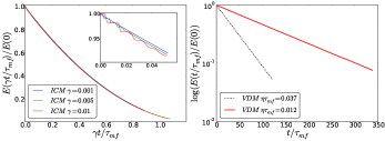
Figure 1: Left: For the ICM, reduced total energy $E(t)/E(0)$ versus $\gamma t/\tau_{mf}$, for the indicated values of $\gamma$ and $R_{0}=0.01$. Inset: zoom on the shorter time evolution. Right: for the VDM, semi-log plot of $E(t)/E(0)$ versus $t/\tau_{mf}$ with the indicated values of $\eta$, and $R_{0}=0.01$.

To explore the validity of this analysis, we have performed a numerical study of two $1D$ self-gravitating systems, i.e. the case $n=-1$ corresponding to the pair potential $\phi(x)=gm|x|$ derived from the 1D Poisson equation $\partial_{x}^{2}\phi(x)=2gm\delta(x)$, one with the dissipation of the ICM, and the other that of the VDM for the case $\alpha=1$. In the absence of dissipation the equations of motion may be integrated exactly between particle collisions (equivalent to crossings), and the system can be evolved using an event-driven algorithmNoullez2003 ; Yawn2003 ; Joyce2011 which determines the collision times exactly (up to round-off errors). For the ICM, inelastic collisions are implemented in an existing code with the appropriate post-collisional velocities (including the coefficient of restitution $c$). For the VDM, an event-driven algorithm is also implemented as the collision time between particles in this case can also be computed exactly by finding the roots of a quintic equation (see Joyce2011 and references therein). We use “rectangular water-bag” initial conditions, i.e., velocities and positions are chosen randomly and uniformly in phase space in $[-v_{0},v_{0}]\times[-L_{0}/2,L_{0}/2]$. These are fully characterized by the initial virial ratio $R_{0}$. We have performed simulations of different sizes ($N=256...4096$), and no noticeable finite effects have been observed. All quantities have been averaged over $100$ independent realizations for the ICM, and $50$ for the VDM (which is less noisy). For both models, the simulation is interrupted when the difference between two possible collision times becomes smaller than the accuracy of the computer.

We define the mean-field time as $\tau_{mf}=2\sqrt{\frac{L_{0}}{gN}}$, and recall the behaviour of this system in absence of dissipation from initial conditions of this kind (as detailed, e.g. in Joyce2010 ): it evolves on a time-scale of order $10-100$ $\tau_{mf}$ towards a QSS, in which the virial ratio $R$ is unity. Monitoring $R$ in the present case (with dissipation) we find essentially identical behaviour, but, as expected, a very different behaviour for the energy. The left panel of Fig. 1 shows, for the ICM, the normalized energy as a function of the dimensionless time $\gamma t/\tau_{mf}$, for an initial virial ratio $R_{0}=0.01$ and the different given values of $\gamma$; in the right panel the same quantity is plotted versus $t/\tau_{mf}$, for the VDM with $\eta\tau_{mf}=0.012,0.037$. We observe excellent agreement with the scaling solutions: for the ICM, the energy decay is fitted by $(1-\frac{t}{t_{c}})^{\delta}$ with $\delta=2.00\pm 0.01$; for the VDM, the energy decay is fitted by $E(t_{s})/E(0)=\exp(-\frac{2}{3}\lambda\frac{t}{\tau_{mf}})$ with $\lambda=\eta\tau_{mf}$, as predicted by the scaling solution (Eqs. (8) and (10)), to $10^{-4}$. The inset of Fig. 1 shows small deviations from the scaling behaviour at short times, associated with the virial oscillations during the initial violent relaxation.

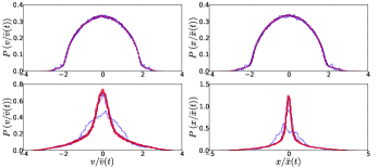
Figure 2: Velocity (left panels) and position (right panels) distributions as a function of rescaled variables, for the ICM with $\gamma=0.01$ at different times $t/\tau_{mf}=10,31,53,74,95$ and $R_{0}=1$ (upper panels) and for the VDM with $\eta\tau_{mf}=0.037$ and $R_{0}=0.01$ (lower panels) at $t/\tau_{mf}=10,20,...,100$.

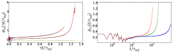
Figure 3: Left: $\phi_{11}$ versus $\gamma t/\tau_{mf}$ for $\gamma=0.01,0.005,0.001$ and $R_{0}=0.01$ (3 upper curves), $R_{0}=0.1$ (3 middle curves) and $R_{0}=1$ (3 lower curves). Right: $\phi_{11}$ versus $t/\tau_{mf}$ in a semi-log plot for $R_{0}=0.01$ and $\gamma=0.001$ (red), $0.005$ (green), $0.01$ (blue)

The velocity and position distributions versus appropriate rescaled variables are shown in Fig. 2 at different times, for the ICM with $R_{0}=1$, and for the VDM with $R_{0}=0.01$. The superposition of the curves illustrates the accurate description of the kinetics by scaling QSS (in the lower panels, the blue curves correspond to $t/\tau_{mf}=10$, in the phase of the violent relaxation). Moreover, one observes significant deviations from a Gaussian shape of the distribution corresponding to the existence of a “core-halo” structure in the QSS Teles_2011 ; PhysRevE.84.011139 .

The ICM is a marginal case for the validity of the approximation in which we obtained the scaling QSS, while for the VDM with $\alpha=1$ and $n=-1$ (i.e. $\beta_{c}=-1$), we expect it to become exact asymptotically. To quantify deviations from the scaling QSS it is convenient to monitor the dimensionless quantity Joyce2010

$$\phi_{11}=\frac{\left\langle|x||v|\right\rangle}{\left\langle|x|\right\rangle\left\langle|v|\right\rangle}-1=\frac{\int|x||v|fdxdv}{\int|x|fdxdv\int|v|fdxdv}-1\,,$$ (11)

which provides a measure of the correlation between the spatial and velocity variables. For conservative self-gravitating systems, $\phi_{11}$ can be interpreted as an order parameter for the QSS, which goes to $0$ as the system goes to thermal equilibriumJoyce2010 . Inserting Eq. (4), in Eq. (11), we see that $\phi_{11}$ is constant in time also in the scaling QSS: the evolution of the system is through a sequence of QSS with identical correlations.

Figure 3, right panel shows the evolution of $\phi_{11}$ for the ICM starting from $R_{0}=0.01$, $R_{0}=0.1$ and $R_{0}=1$, and for the three different values of $\gamma$. We have used here this rescaled time $\gamma t/\tau_{mf}$ because we observe that it gives a good collapse of all curves; on the left panel, the result for the first case ($R_{0}=0.01$) is shown without this rescaling. For the VDM (not shown here) $\phi_{11}$ remains constant (after the initial violent relaxation). We observe that while the case $R_{0}=1$, $\phi_{11}$ is almost constant, visible deviations are evident for the two other cases, with evolution away from the scaling setting in fastest for the case $R_{0}=0.01$. Similarly, the space and velocity distributions deviate progressively from the scaling solutions for $R_{0}=0.1,0.01$ (not shown here). In both cases, the system energy decreases as predicted by the scaling solution. Moreover, this evolution appears to depend only on the QSS attained (which is different for each $R_{0}$), and on $\gamma$ through the rescaled variable. Thus, as the total energy goes to $0$, inelastic collisions drive the system through a given family of ever more correlated QSS. It implies that the system never shows any tendency to drive the system towards a Maxwell-Boltzmann distribution of velocities (nor towards the spatial distribution of the thermal equilibrium of the model), despite the effective stochasticity of the inelastic collisions. This contrasts to what is observed in a stochastically perturbed HMF model in PhysRevLett.105.040602 ; Gupta2010 . This tendency towards more correlated states can be interpreted as follows: for $R_{0}\ll 1$, the violent relaxation drives the system to a core-halo structure (see PhysRevLett.100.040604 ; Joyce2010 ; Teles_2011 ), whereas for $R_{0}\simeq 1$, the QSS is rather homogeneous in phase space. For the ICM, the (kinetic) temperature of the core decreases more rapidly than that of the halo; in the VDM, on the other hand, the systems cools down uniformly. Further it may be, as observed in three dimensional gravitating systems Ispolatov2004 , that inefficiency of energy exchange between the core and halo impedes relaxation towards thermal equilibrium.

The authors thank C. Rulquin for useful remarks.

References

- (1) A. Campa, T. Dauxois, and S. Ruffo, Phys. Rep. 480, 57 (2009)
- (2) F. Bouchet, S. Gupta, and D. Mukamel, Physica A 389, 4389 (2010)
- (3) Y. Levin, R. Pakter, and T. N. Teles, Phys. Rev. Lett. 100, 040604 (2008)
- (4) A. Antoniazzi, Y. Elskens, D. Fanelli, and S. Ruffo, Eur. Phys. J. B 50, 603 (2006)
- (5) M. Chalony, J. Barré, B. Marcos, A. Olivetti, and D. Wilkowski, Phys. Rev. A 87, 013401 (2013)
- (6) J. Sopik, C. Sire, and P.-H. Chavanis, Phys. Rev. E 72, 026105 (2005)
- (7) J. Binney and S. Tremaine, Galactic Dynamics, 2nd ed. (Princeton University Press, 2008)
- (8) F. Bouchet and J. Sommeria, Journal of Fluid Mechanics 464, 165 (2002)
- (9) M. Antoni and S. Ruffo, Phys. Rev. E 52, 2361 (1995)
- (10) F. Baldovin, P.-H. Chavanis, and E. Orlandini, Phys. Rev. E 79, 011102 (2009)
- (11) P.-H. Chavanis, F. Baldovin, and E. Orlandini, Phys. Rev. E 83, 040101 (2011)
- (12) S. Gupta and D. Mukamel, Phys. Rev. Lett. 105, 040602 (2010)
- (13) S. Gupta and D. Mukamel, J. Stat. Mech. 2010, P08026 (2010)
- (14) A. Gabrielli, M. Joyce, and B. Marcos, Phys. Rev. Lett. 105, 210602 (2010)
- (15) M. Joyce and F. Sicard, Mon. Not. R. Astron. Soc 413, 1439 (2011)
- (16) P. Martin and J. Piasecki, J. Stat. Phys. 84, 837 (1996)
- (17) P. K. Haff, J. Fluid Mech. 134, 401 (1983)
- (18) I. Goldhirsch and G. Zanetti, Phys. Rev. Lett. 70, 1619 (1993)
- (19) I. Fouxon, B. Meerson, M. Assaf, and E. Livne, Phys. Fluids 19, 093303 (2007)
- (20) S. F. Shandarin and Y. B. Zeldovich, Rev. Mod. Phys. 61, 185 (1989)
- (21) I. S. Aranson and L. S. Tsimring, Rev. Mod. Phys. 78, 641 (2006)
- (22) P.-H. Chavanis, J. Stat. Mech. 2010, P05019 (2010)
- (23) M. E. Tuckerman, C. J. Mundy, and G. J. Martyna, Europhys. Lett. 45, 149 (1999)
- (24) V. I. Arnold, Mathematical methods of classical mechanics (Springer-Verlag, New York, 1989)
- (25) T. Pöschel and N. Brilliantov, Granular Gas Dynamics (Springer, Berlin, 2003)
- (26) J. Talbot, R. D. Wildman, and P. Viot, Phys. Rev. Lett. 107, 138001 (2011)
- (27) S. McNamara and W. R. Young, Phys. Fluids: A 5, 34 (1993)
- (28) S. Aumaitre, A. Alastuey, and S. Fauve, Eur. Phys. J. B 54, 263 (2006)
- (29) A. Noullez, D. Fanelli, and E. Aurell, J Comput Phys 186, 697 (2003)
- (30) K. R. Yawn and B. N. Miller, Phys. Rev. E 68, 056120 (2003)
- (31) M. Joyce and T. Worrakitpoonpon, J. Stat. Mech. 2010, P10012 (2010)
- (32) T. N. Teles, Y. Levin, and R. Pakter, Mon. Not. R. Astron. Soc 417, L21 (2011)
- (33) M. Joyce and T. Worrakitpoonpon, Phys. Rev. E 84, 011139 (2011)
- (34) I. Ispolatov and M. Karttunen, Phys. Rev. E 70, 026102 (2004)