Photon-Assisted Tunneling through Molecular Conduction Junctions with Graphene Electrodes.

Abstract

Graphene electrodes provide a suitable alternative to metal contacts in molecular conduction nanojunctions. Here, we propose to use graphene electrodes as a platform for effective photon assisted tunneling through molecular conduction nanojunctions. We predict dramatic increasing currents evaluated at side-band energies $\sim n\hbar\omega$ ($n$ is a whole number) related to the modification of graphene gapless spectrum under the action of external electromagnetic field of frequency $\omega$. A side benifit of using doped graphene electrodes is the polarization control of photocurrent related to the processes occurring either in the graphene electrodes or in the molecular bridge. The latter processes are accompanied by surface plasmon excitation in the graphene sheet that makes them more efficient. Our results illustrate the potential of graphene contacts in coherent control of photocurrent in molecular electronics, supporting the possibility of single-molecule devices.

I Introduction

The field of molecular-scale electronics has been rapidly advancing over the past two decades, both in terms of experimental and numerical technology and in terms of the discovery of new physical phenomena and realization of new applications (for recent reviews please see Refs.Kohler05 ; Chen09 ; Heath09 ). In particular, the optical response of nanoscale molecular junctions has been the topic of growing experimental and theoretical interest in recent years Park11PRB ; Wang11PCCP ; Fainberg_Galperin11PRB ; Haertle10JCP ; Reuter08PRL ; Li08SSP ; Thanopulos08Nanotech ; Prociuk08PRB ; Li08NJP ; Galperin08JCP ; Li07EPL ; Fai07PRB , fueled in part by the rapid advance of the experimental technology and in part by the premise for long range applications in optoelectronics.

A way of the control of the current through molecular conduction nanojunctions is the well-known photon-assisted tunneling (PAT) Platero04 ; Kohler05 that was studied already in the early 1960’s experimentally by Dayem and Martin Dayem_Martin62PRL and theoretically by Tien and Gordon using a simple theory which captures already the main physics of PAT Tien_Gordon63 . The main idea is that an external field periodic in time with frequency $\omega$ can induce inelastic tunneling events when the electrons exchange energy quanta $\omega$ with the external field. PAT may be related either to the potential difference modulation between the contacts of the nanojunction when electric field is parallel to the axis of a junction Tien_Gordon63 ; Gri98 ; Platero04 ; Kleinekathofer06EPL ; Li07EPL , or to the electromagnetic (EM) excitation of electrons in the metallic contacts when electric field is parallel to the film surface of contacts Tien_Gordon63 . According to the Tien-Gordon model Tien_Gordon63 ; Platero04 ; Li07EPL for monochromatic external fields that set up a potential difference $V(t)=V_{0}\cos\omega t$, the rectified dc currents through ac-driven molecular junctions are determined as Platero04 ; Li07EPL

$$I_{TG}=\sum_{n=-\infty}^{\infty}J_{n}^{2}(\frac{eV_{0}}{\hbar\omega})I_{dc}^{0}(eV_{0}+n\hbar\omega)=\sum_{n=-\infty}^{\infty}I_{n}$$ (1)

where the current in the driven system is expressed by a sum over contributions of the current $I_{dc}^{0}(eV_{0}+n\hbar\omega)$ in the undriven case but evaluated at side-band energies $eV_{0}+n\hbar\omega$ shifted by integer multiples of the photon quantum and weighted with squares of Bessel functions. A formula similar to Eq.(1) can be obtained also for EM excitation of electrons in the metallic contacts Tien_Gordon63 . Note that the partial currents $I_{n}$ contain contributions from $\pm n$. The term $J_{n}(\frac{eV_{0}}{\hbar\omega})$ denotes the $n$-th-order Bessel function of the first kind. The photon absorption ($n>0$) and emission ($n<0$) processes can be viewed as creating effective electron densities at energies $eV_{0}\pm n\hbar\omega$ with probability $J_{n}^{2}(\frac{eV_{0}}{\hbar\omega})$. These probabilities strongly diminish with number $n$ when $eV_{0}\leq\hbar\omega$ that severely sidelines the control of the current for not strong EM fields ($<10^{6}$ $V/cm$ Kohler05 ).

In the last time graphene, a single layer of graphite, with unusual two-dimensional Dirac-like electronic excitations, has attracted considerable attention due to its exceptional electronic properties (ballistic in-plane electron transport etc.) Novoselov09RMP ; Trauzettel07PRB ; Efetov08PRB . Quite recently they have shown interest to a new kind of graphene-molecule-graphene (GMG) junctions that may exhibit unique physical properties, including a large conductance (achieving $0.38$ conductance quantum), and are potentially useful as electronic and optoelectronic devices Yang_graphene_junctions10JCP . The junction consists of a conjugated molecule connecting two parallel graphene sheets. In this relation it would be interesting to investigate PAT in such a junction to control the current through it. The PAT in GMG junctions under EM excitation of electrons and holes in the graphene contacts may be rather different from that for usual metallic contacts. It was shown that the massless energy spectrum of electrons and holes in graphene led to the strongly non-linear EM response of this system, which could work as a frequency multiplier Mikhailov07EPL . The predicted efficiency of the frequency up-conversion was rather high: the amplitudes of the higher-harmonics of the ac electric current fell down slowly (as $1/n$) with harmonics index $n$. Sure, the strongly non-linear EM response should also lead to a slow falling down currents evaluated at side-band energies $\sim n\hbar\omega$ (see Eq.(1)) with harmonics index $n$ in comparison to nanojunctions with metallic (or semiconductor Fainberg13CPL ) leads (see below). This makes controlling charge transfer essentially more effective than that for molecular nanojunctions with metallic contacts. Additional factors that may enhance currents evaluated at side-band energies $\sim n\hbar\omega$ in nanojunctions with graphene electrodes are linear dependence of the density of states on energy in graphene Novoselov09RMP , and the gapless spectrum of graphene that can change under the action of external EM field (see below).

Here we propose and explore theoretically a new approach to coherent control of electric transport via molecular junctions, using either both graphene electrodes or one graphene and another one - a metal electrode (that may be an STM tip). Our approach is based on the excitation of dressed states of the doped graphene electrode with electric field that is parallel to its surface, having used unique properties of graphene mentioned above. As a first step, we calculate a semiclassical wave function of a doped graphene under the action of EM excitation. Then we obtain Heisenberg equations for the second quantization operators of graphene and calculate current through a molecular junction with graphene electrodes using non-equilibrium Green functions (GF). We address different cases, which are analytically soluble, hence providing useful insights. We show that using graphene electrodes can essentially enhance currents evaluated at side-band energies $\sim n\hbar\omega$ in molecular nanojunctions.

II Model Hamiltonian

Consider a spinless model for a molecular wire that comprises one site of energy $\varepsilon_{m}$, positioned between either both graphene electrodes (leads) (Fig.1) or one graphene and another one - a metal electrode (Fig.2).

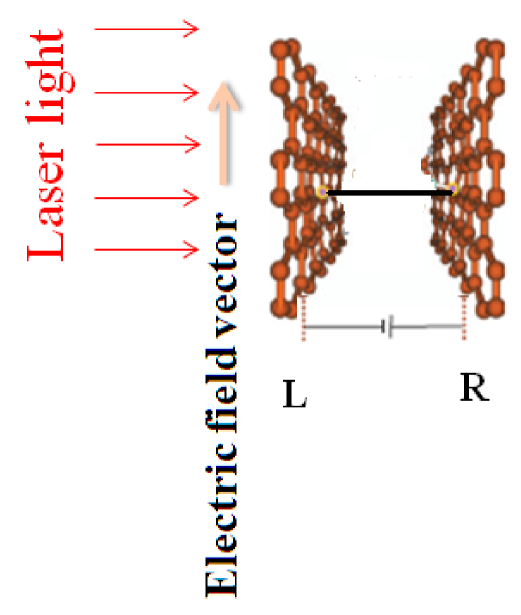
Figure 1: Molecular bridge ( thick horizontal line) between left (L) and right (R) graphene electrodes with applied voltage bias. External electromagnetic field acts on the electrodes.

The leads are represented by electron reservoirs $L$ and $R$, characterized by the electronic chemical potentials $\mu_{K}$, $K=L,R$, and by the ambient temperature $T$. The corresponding Fermi distributions are $f_{K}(\varepsilon_{k})=[\exp((\varepsilon_{k}-\mu_{K})/k_{B}T)+1]^{-1}$ in the absense of external EM field, and the difference $\mu_{L}-\mu_{R}$ $=e\varphi_{0}$ is the imposed voltage bias between the electrodes. External EM field acting on electrode $K$, $\mathbf{E}(t)=\mathbf{E}_{0}\cos\omega t$, changes the corresponding Fermi distribution (see below). The Fermi energy of the graphene electrode may be controlled via electrical or chemical modification of the charge carrier density Mak08PRL ; Chen8Nature ; Abajo11NL ; Chen12Nature ; Fei12Nature . We consider that steady-state current through a nanojunction does not influence on the Fermi energy, since such current does not change a charge of the graphene electrode.

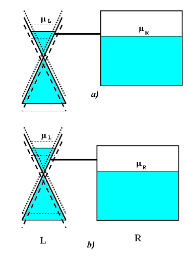
Figure 2: Molecular bridge between n-doped graphene (left-L) and metal (right-R) electrodes. Thick horizontal line - energy of the molecular bridge $\varepsilon_{m}$, $\mu_{L\text{ }}$ and $\mu_{R\text{ }}=\mu-e\varphi_{0}/2$ - chemical potentials of the left and right leads, respectively, in the biased junction. The energy spectrum of unperturbated graphene is shown by the solid line; dotted and dashed lines show the upper and lower first photonic replica of the graphene spectrum, repectively, that are displaced an amount $\hbar\omega$ from unperturbated spectrum. Solid thin horizontal line - chemical potential of unperturbated graphene $\mu_{L\text{ }}=\mu+e\varphi_{0}/2$, dashed thin horizontal lines - chemical potentials of the photonic replica $\mu_{L\text{ }}=\mu+e\varphi_{0}/2\pm\hbar\omega$. a - potential of the graphene electrode is smaller than photon energy, $e\varphi_{0}/2<\hbar\omega$; b - potential of the graphene electrode is larger than photon energy, $e\varphi_{0}/2>\hbar\omega$. The lower photonic replication gives contribution into the current only in case b) that causes the step shown in Fig.3.

The corresponding Hamiltonian is

$$\hat{H}_{junction}=\hat{H}_{wire}+\hat{H}_{leads}+\hat{V}$$ (2)

where the wire Hamiltonian is $\hat{H}_{wire}=\varepsilon_{m}\hat{c}_{m}^{{\dagger}}\hat{c}_{m}$, $\hat{c}_{m}^{{\dagger}}$ ($\hat{c}_{m}$) are creation (annihilation) operators for electrons at the molecular wire. The molecule-leads interaction $\hat{V}$ describes electron transfer between the molecular bridge and the right ($R$) and left ($L$) leads that gives rise to net current in the biased junction

$$\hat{V}=\sum_{+,-}\sum_{\sigma,\mathbf{p}\in\{L,R\}}(V_{\mathbf{p\pm,}\sigma;m}\hat{a}_{\mathbf{p\pm,}\sigma}^{{\dagger}}\hat{c}_{m}+H.c.)$$ (3)

Here $H.c.$ denotes Hermitian conjugate, $\hat{a}_{\mathbf{p\pm,}\sigma}^{{\dagger}}$ are creation operators for graphene electrodes (see below). The corresponding contribution to $\hat{V}$ from a metal electrode does not contain summation with respect to positive and negative energies ($\pm$) and quasispin index $\sigma$.

III Calculation of Semiclassical Wave Function

The states of electrons in graphene are conveniently described by the four-component wave functions, defined on two sublattices and two valleys. Electron motion in the time-dependent EM field is described by the 2D Dirac equation Novoselov09RMP ; Efetov08PRB

$$i\hbar\frac{\partial\mathbf{\psi}}{\partial t}=[v\mathbf{\hat{\sigma}}(\mathbf{\hat{p}}-\frac{e}{c}\mathbf{A})+e\varphi_{pot}]\mathbf{\psi}$$ (4)

written for a single valley and for a certain direction of spin. Here $\mathbf{\hat{p}}$ is the momentum of the quasiparticle, $v$ - the Fermi velocity ($v\approx 10^{6}$ m/s), $\mathbf{\hat{\sigma}}$ - the vector of the Pauli matrices in the sublattice space (“pseudospin” space), $\mathbf{A}$ and $\varphi_{pot}$ are vector and scalar potentials of an EM field, respectively. Suppose a graphene film is excited by a linearly polarized monochromatic electric field $E_{x}(t)=E_{0}\cos\omega t$ that is parallel to its plane ($x,y$). Then $A_{x}=-(c/\omega)E_{0}\sin\omega t$, $A_{y}=A_{z}=0$. Eq.(4) can be brought to more symmetric form $i[\hat{P}-(e/c)\hat{A}]\mathbf{\psi=}0,$ introducing matrices $\gamma_{1}=\hat{\sigma}_{y},\gamma_{2}=-\hat{\sigma}_{x}$ and $\gamma_{3}=\hat{\sigma}_{z}$, where

$$\hat{P}=-i\hbar{\displaystyle\sum\limits_{k=1}^{3}}\gamma_{k}\frac{\partial}{\partial x_{k}},\text{ }\hat{A}={\displaystyle\sum\limits_{k=1}^{3}}\gamma_{k}A_{x_{k}},$$ (5)

$x_{1}=x$, $x_{2}=y$, $x_{3}=ivt$ and $A_{x_{3}}=i\frac{c}{v}\varphi_{pot}$. To obtain a semiclassical solution of Eq.(4), we shall use a method of Ref. Pauli32 (see also akhiezer-berestetskii69 ). Let us put $\mathbf{\psi}=-i(\hat{P}-\frac{e}{c}\hat{A})\Phi$. Then one can obtain the following equation for $\Phi$

$$[i\frac{\hbar e}{2c}{\displaystyle\sum\limits_{k,l=1}^{3}}\gamma_{k}\gamma_{l}(1-\delta_{kl})F_{x_{l}x_{k}}-{\displaystyle\sum\limits_{k=1\ }^{3}}(\hbar\frac{\partial}{\partial x_{k}}-i\frac{e}{c}A_{x_{k}})^{2}]\Phi=0$$ (6)

where $F_{x_{l}x_{k}}=\partial A_{x_{l}}/\partial x_{k}-\partial A_{x_{k}}/\partial x_{l}$ is the field tensor. Let us seek a solution of Eq.(6) as an expansion in power series in $\hbar$

$$\mathbf{\Phi=}\exp(iS/\hbar)w=\exp(iS/\hbar)(w_{0}+\hbar w_{1}+\hbar^{2}w_{2}+...)$$ (7)

where $S$ is a scalar and $w$ is a slowly varying spinor berestetskii-lifshitz99 . Substituting series, Eq.(7), into Eq.(6) and collecting coefficients at the equal exponents of $\hbar$, we get that $S$ is the action obeying the Hamilton-Jacobi equation $\partial S/\partial t=-H$ where $H$ is the classical Hamilton function of a particle:

$$\exp(\frac{i}{\hbar}S)=\exp[-\frac{i}{\hbar}(v\int_{0}^{t}\sqrt{\bar{p}_{x}^{2}+\bar{p}_{y}^{2}}dt^{\prime}+e\int_{0}^{t}\varphi_{pot}dt^{\prime})],$$ (8)

and the equation for spinor $w_{0}$

$${\displaystyle\sum\limits_{k=1\ }^{3}}\{[\frac{\partial}{\partial x_{k}}(\frac{\partial S}{\partial x_{k}}-\frac{e}{c}A_{x_{k}})]w_{0}+2(\frac{\partial S}{\partial x_{k}}-\frac{e}{c}A_{x_{k}})\frac{\partial w_{0}}{\partial x_{k}}-\frac{e}{2c}{\displaystyle\sum\limits_{l=1}^{3}}\gamma_{k}\gamma_{l}(1-\delta_{kl})F_{x_{l}x_{k}}w_{0}\}=0$$ (9)

In Eq.(8), $\mathbf{\bar{p}}$ is the normal momentum that obeys the classical equations of motion $d\bar{p}_{x}/dt=-eE_{x}(t)$ for a particle with charge $-e$, according to which $\bar{p}_{x}(t)=-(eE_{0}/\omega)\sin(\omega t)$; $\mathbf{\bar{p}=p}-\frac{e}{c}\mathbf{A}$ where $\mathbf{p}$ is the generalized momentum. If one takes only the first term in series, Eq.(7), into account, it can be shown that wave packets behave like particles moving along classical trajectories.

Let us solve Eq.(9) for spinor $w_{0}$. We shall introduce a linear combination of the components of the Hermitian conjugated wave function $\mathbf{\psi}^{{\dagger}}$ by $\mathbf{\bar{\psi}}=\mathbf{\psi}^{{\dagger}}\gamma_{3}$ akhiezer-berestetskii69 . Then using equation $\mathbf{\psi}=-i(\hat{P}-\frac{e}{c}\hat{A})\Phi$ and Eqs.(5), one can show that electronic flux $s_{k}=i\mathbf{\bar{\psi}}\gamma_{k}\mathbf{\psi}$ obeys the continuity equation

$${\displaystyle\sum\limits_{k=1}^{3}}\frac{\partial}{\partial x_{k}}s_{k}=0$$ (10)

Put

$$w_{0}=\sqrt{\xi}\varphi_{0}$$ (11)

where we denoted

$$\xi=-i2\bar{w}_{0}\hat{\pi}w_{0}$$ (12)

and $\hat{\pi}={\displaystyle\sum\limits_{k=1}^{3}}\gamma_{k}\pi_{k}$, $\pi_{k}=\partial S/\partial x_{k}-(e/c)A_{x_{k}}$. Then in our approximation the electronic flux is reduced to $s_{k}=\pi_{k}\xi$ that gives, bearing in mind Eq.(10),

$${\displaystyle\sum\limits_{k=1}^{3}}\frac{\partial}{\partial x_{k}}(\pi_{k}\xi)=0$$ (13)

Here quantities $\pi_{k}$ can be written as $\pi_{k}=\bar{p}_{k},$ $k=1,2$ and $\pi_{3}=\pm i\bar{p}$ with the aid of the Hamilton-Jacobi equation $\partial S/\partial t=-H$ and $\partial S/\partial x_{k}=p_{k},$ $k=1,2$. Here signs plus and minus are related to positive and negative energies, respectively. Eq.(13) can be write over as

$${\displaystyle\sum\limits_{k=1\ }^{3}}(\frac{\partial\pi_{k}}{\partial x_{k}}\xi+\pi_{k}\frac{\partial\xi}{\partial x_{k}})=0$$ (14)

Using Hamilton’s equations $\dot{x}_{k}=\partial H/\partial p_{k},$ $k=1,2,$ the time derivative $\dot{x}_{k}$ can be written as

$$\dot{x}_{k}=\pm v\frac{\bar{p}_{k}}{\bar{p}}=iv\frac{\pi_{k}}{\pi_{3}},\text{ }k=1,2$$ (15)

This enables us to write down the second term on the right-hand side of Eq.(14) in the form

$${\displaystyle\sum\limits_{k=1\ }^{3}}\pi_{k}\frac{\partial\xi}{\partial x_{k}}=-\frac{i\pi_{3}}{v}[{\displaystyle\sum\limits_{k=1\ }^{2}}\frac{\partial\xi}{\partial x_{k}}\frac{dx_{k}}{dt}+\frac{\partial\xi}{\partial t}]=-\frac{i\pi_{3}}{v}\frac{d\xi}{dt}$$

and Eq.(14) becomes

$$\frac{d\xi}{dt}=-\frac{1}{\bar{p}}\frac{\partial\bar{p}}{\partial t}\xi$$ (16)

since $\partial\pi_{k}/\partial x_{k}=0$ for $k=1,2$. Integrating Eq.(16), one gets

$$\xi(t)=\xi(0)\frac{\bar{p}(0)}{\bar{p}(t)}$$ (17)

where $\bar{p}(0)=p$. Furthermore, substituting Eq.(11) into Eq.(9), we obtain equation for spinor $\varphi_{0}=\left(\begin{array}[c]{c}\varphi_{01}\\ \varphi_{02}\end{array}\right)$: $\frac{d\varphi_{0}}{dt}=\pm\frac{e}{2\bar{p}}\mathbf{\hat{\sigma}E}\varphi_{0}$, the solution of which may be written as

$$\varphi_{01,2} =\frac{1}{2\sqrt{p\bar{p}(1+\cos\varphi)(1+\cos\bar{\varphi})}}\{\varphi_{01,2}(0)[\bar{p}(1+\cos\bar{\varphi})+$$

$$+p(1+\cos\varphi)]\pm\varphi_{02,1}(0)[\bar{p}(1+\cos\bar{\varphi})-p(1+\cos\varphi)]\}$$ (18)

The quantities $\xi(0)$ and $\varphi_{01,2}(0)$ in Eqs.(17) and (18) are chosen in such a way that the wave function $\mathbf{\psi}=\exp(\frac{i}{\hbar}S)(-i\hat{\pi})\sqrt{\xi}\varphi_{0}$ should be normalized and coincide with the wave function of unperturbated graphene in the absence of external EM field Novoselov09RMP . After combersome calculations we get the wave function normalized for the graphene sheet area $s$:

$$\psi =\frac{1}{\sqrt{s}}\exp(ip_{x}x/\hbar+ip_{y}y/\hbar)\exp[\frac{i}{\hbar}(\mp v\int_{0}^{t}\bar{p}dt^{\prime}-$$

$$-e\int_{0}^{t}\varphi_{pot}dt^{\prime})]\bar{u}_{\mathbf{p\pm}}$$ (19)

where slowly varying spinors $\bar{u}_{\mathbf{p\pm}}$ are equal to

$$\bar{u}_{\mathbf{p\pm}}\mathbf{=}\frac{1}{\sqrt{2}}\left(\begin{array}[c]{c}\exp(-i\bar{\varphi}/2)\\ \pm\exp(i\bar{\varphi}/2)\end{array}\right),$$ (20)

$\bar{p}\equiv\left|\mathbf{\bar{p}}(t)\right|$, $\tan\bar{\varphi}=\bar{p}_{y}/\bar{p}_{x}$, $p_{x}=p\cos\varphi$, $p_{y}=p\sin\varphi$, $\tan\varphi=p_{y}/p_{x}$.

Eqs.(19) and (20) show remarkable and very simple result, according to which the time-dependent part of the semiclassical wave function is defined by the same formula as that for the unperturbated system with the only difference that the generalized momentum $\mathbf{p}$ should be replaced by the usual momentum $\mathbf{\bar{p}}$. The space-dependent part of the wave function remains unchanged.

III.1 Heisenberg Equations for the Second Quantization Operators of Graphene

The wave function of the graphene sheet interacting with molecular bridge $\Psi$ may be represented as the superposition of wave functions, Eqs.(19) and (20). Passing to the second quantization, we get

$$\Psi =\frac{1}{\sqrt{s}}{\displaystyle\sum\limits_{+,-}}{\displaystyle\sum\limits_{\mathbf{p}}}\hat{a}_{\mathbf{p\pm}}\exp[\frac{i}{\hbar}\mathbf{pr}+\frac{i}{\hbar}(\mp v\int_{0}^{t}\bar{p}dt^{\prime}$$

$$-e\int_{0}^{t}\varphi_{pot}dt^{\prime})]\bar{u}_{\mathbf{p\pm}}$$ (21)

where $\hat{a}_{\mathbf{p\pm}}$ are annihilation operators. To obtain the Hamiltonian in the second quantization representation, consider an average energy of a particle with wave function $\psi$ that is given by $\int\psi^{\ast}\hat{H}\psi d\mathbf{r=}i\hbar\int\psi^{\ast}(\partial\psi/\partial t)d\mathbf{r}$. Replacing wave functions $\psi$ for $\Psi$ operators and integrate with respect to $\mathbf{r}$, we get

$$\hat{H}=\int\Psi^{{\dagger}}\hat{H}\Psi d\mathbf{r}={\displaystyle\sum\limits_{\mathbf{p\sigma}}}{\displaystyle\sum\limits_{+,-}}\hat{a}_{\mathbf{p\pm,}\sigma}^{{\dagger}}\hat{a}_{\mathbf{p\pm,}\sigma}[\pm v\bar{p}(t)+e\varphi_{pot}(t)]$$ (22)

where $\sum_{\sigma}\hat{a}_{\mathbf{p\pm,}\sigma}^{{\dagger}}\hat{a}_{\mathbf{p\pm,}\sigma}=\hat{a}_{\mathbf{p\pm}}^{{\dagger}}\hat{a}_{\mathbf{p\pm}},$ $\sigma=1,2$ is the ”quasispin” index. In deriving Eq.(22), we have taken into account that the main contribution to $\partial\Psi/\partial t$ in the semiclassical approximation is given by the exponential term on the right-hand side of Eq.(21) (see Ref.landau-lifshitz.65 , chapter II). In addition, we beared in mind that the summation over $\mathbf{p}$ can be substituted by the integration over phase space $d\Gamma=d\mathbf{p}d\mathbf{r}$

$${\displaystyle\sum\limits_{\mathbf{p}}}\rightarrow\int\frac{d\Gamma}{(2\pi\hbar)^{2}}=\frac{s}{(2\pi\hbar)^{2}}\int d\mathbf{p}$$ (23)

Using Hamiltonian, Eq.(22), we obtain the Heisenberg equations of motion

$$\frac{d\hat{a}_{\mathbf{p\pm,}\sigma}(t)}{dt}=\frac{i}{\hbar}[\hat{H},\hat{a}_{\mathbf{p\pm,}\sigma}]\mathbf{\simeq}\frac{i}{\hbar}[\mp v\bar{p}(t)-e\varphi_{pot}(t)]\hat{a}_{\mathbf{p\pm,}\sigma}(t)$$ (24)

IV Formula for the Current

The current from the $K$ lead ($K=L,R$) can be obtained by the generalization of Eq.(12.11) of Ref.haug-jauho.96

$$I_{K}=-\frac{2\varkappa e}{\hbar}\operatorname{Re}\sum_{+,-}\sum_{\sigma,\mathbf{p}\in K}V_{\mathbf{p\pm,}\sigma;m}G_{m;\mathbf{p\pm,}\sigma}^{<}(t,t)$$ (25)

where $\varkappa=1$ for the metal electrode, and $\varkappa=2$ for the graphene electrode that accounts for the valley degeneracies of the quasiparticle spectrum in graphene. $G_{m;\mathbf{p\pm,}\sigma}^{<}(t,t^{\prime})=i\langle\hat{a}_{\mathbf{p\pm,}\sigma}^{{\dagger}}(t^{\prime})\hat{c}_{m}(t)\rangle$ denotes the lesser GF that is given by

$$G_{m;\mathbf{p\pm,}\sigma}^{<}(t,t^{\prime}) =\frac{1}{\hbar}\int dt_{1}V_{\mathbf{p\pm,}\sigma;m}^{\ast}[G_{mm}^{r}(t,t_{1})g_{\mathbf{p\pm,}\sigma}^{<}(t_{1},t^{\prime})+$$

$$+G_{mm}^{<}(t,t_{1})g_{\mathbf{p\pm,}\sigma}^{a}(t_{1},t^{\prime})]$$ (26)

where $G_{mm}^{r}(t,t_{1})$ and $G_{mm}^{<}(t,t_{1})$ are the retarded and lesser wire GFs, respectively; $g_{\mathbf{p\pm,}\sigma}^{<}(t,t^{\prime})=i\langle\hat{a}_{\mathbf{p\pm,}\sigma}^{{\dagger}}(t^{\prime})\hat{a}_{\mathbf{p\pm,}\sigma}(t)\rangle$ and $g_{\mathbf{p\pm,}\sigma}^{a}(t_{1},t^{\prime})=i\theta(t^{\prime}-t_{1})\langle\{\hat{a}_{\mathbf{p\pm,}\sigma}(t_{1}),\hat{a}_{\mathbf{p\pm,}\sigma}^{{\dagger}}(t^{\prime})\}\rangle$ are the lesser and advanced lead GFs, respectively; $\theta(t^{\prime}-t_{1})$ is the unit function. Using Eq.(24), we get

$$g_{\mathbf{p\pm,}\sigma}^{<}(t,t^{\prime}) =i\langle\hat{a}_{\mathbf{p\pm,}\sigma}^{{\dagger}}(t^{\prime})\hat{a}_{\mathbf{p\pm,}\sigma}(t)\rangle=if^{K}(vp_{\pm})\times$$

$$\times\exp\{\frac{i}{\hbar}[-e\varphi_{pot,K}(t-t^{\prime})\mp v\int_{t^{\prime}}^{t}dt^{\prime\prime}\bar{p}(t^{\prime\prime})]\}$$ (27)

and

$$g_{\mathbf{p\pm,}\sigma}^{a}(t_{1},t^{\prime}) =i\theta(t^{\prime}-t_{1})\exp\{\frac{i}{\hbar}[-e\varphi_{pot,K}(t_{1}-t^{\prime})$$

$$\mp v\int_{t^{\prime}}^{t_{1}}dt^{\prime\prime}\bar{p}(t^{\prime\prime})]\}$$ (28)

where $f^{K}(vp_{\pm})$ $\equiv\langle\hat{a}_{\mathbf{p\pm,}\sigma}^{{\dagger}}(0)\hat{a}_{\mathbf{p\pm,}\sigma}(0)\rangle=\left[1+\exp\left(\frac{\pm vp-\mu_{K}}{k_{B}T}\right)\right]^{-1}$ is the Fermi function and $\mu_{K}$ - the chemical potential of lead $K$. Substituting Eqs.(26), (27) and (28) into Eq.(25), and converting the momentum summations to energy integration, Eq.(23), we get

$$I_{K} =\frac{4e}{\hbar}\int_{-\infty}^{t}dt_{1}\sum_{+,-}\operatorname{Im}\int_{0}^{\infty}\frac{d(vp)}{2\pi}\exp[\pm\frac{i}{\hbar}e\varphi_{pot,K}(t-t_{1})]\times$$

$$\times\Gamma_{mm}^{K}(\pm vp,t_{1,}t)[G_{mm}^{r}(t,t_{1})f^{K}(\pm vp)+G_{mm}^{<}(t,t_{1})]$$ (29)

where

$$\Gamma_{mm}^{K}(\pm vp,t_{1,}t) =\frac{2\pi}{\hbar}\left(\frac{s}{2\pi^{2}\hbar v^{2}}\right)\sum_{\sigma\in K}\int_{0}^{\pi}d\theta vpV_{\mathbf{p\pm,}\sigma;m}(t)\times$$

$$\times V_{\mathbf{p\pm,}\sigma;m}^{\ast}(t_{1})\exp[\pm\frac{i}{\hbar}v\int_{t_{1}}^{t}dt^{\prime}\bar{p}(t^{\prime})]$$ (30)

is the level-width function.

To proceed, we shall make the time expansion of $\Gamma_{mm}^{K}(\pm vp,t_{1,}t)$ into the Fourier series, and then use the Markovian approximation, considering time $t-t_{1}\equiv\tau$ as very short. This will also enable us to use the non-interacting resonant-level model haug-jauho.96 for finding the time dependence of $G_{mm}^{r}(t,t-\tau)=-i\theta(\tau)\exp(-\frac{i}{\hbar}\varepsilon_{m}\tau)$ and $G_{mm}^{<}(t,t-\tau)=in_{m}(t)\exp(-\frac{i}{\hbar}\varepsilon_{m}\tau)$ as functions of $t$ and $t-\tau$ where $n_{m}(t)$ is the population of molecular state $m$.

According to the Floquet theorem Kohler05 , the general solution of the Schrödinger equation for an electron subjected to a periodic perturbation, takes the form $\psi(t)=\exp(-\frac{i}{\hbar}\varepsilon t)\Phi_{T}(t)$, where $\Phi_{T}(t)$ is a periodic function having the same period $T$ as the perturbation, and $\varepsilon$ is called quasienergy. Then the expansion of function $\exp[\frac{i}{\hbar}v\int_{0}^{t}dt^{\prime}\bar{p}(t^{\prime})]$ on the right-hand side of Eq.(19) into the Fourier series will be as following

$$\exp[\frac{i}{\hbar}v\int_{0}^{t}dt^{\prime}\bar{p}(t^{\prime})]=\exp[\frac{i}{\hbar}\varepsilon(p,\theta)t]{\displaystyle\sum\limits_{l=-\infty}^{\infty}}c_{l}(p,\theta)\exp(ilt\omega)$$ (31)

where

$$c_{l}(p,\theta)=\frac{\omega}{2\pi}\int_{-\pi/\omega}^{\pi/\omega}\exp[\frac{i}{\hbar}v\int_{0}^{t}dt^{\prime}\bar{p}(t^{\prime})-\frac{i}{\hbar}\varepsilon(p,\theta)t-il\omega t]dt$$ (32)

Using expansion, Eq.(31), into Eq.(30) and neglecting fast oscillating with time $t$ terms, we get

$$\Gamma_{mm}^{K}(\pm vp,\tau) =\frac{2\pi}{\hbar}\left(\frac{s}{2\pi^{2}\hbar v^{2}}\right)\sum_{\sigma\in K}\int_{0}^{\pi}d\theta vp|V_{\mathbf{p\pm,}\sigma;m}|^{2}\times$$

$$\times{\displaystyle\sum\limits_{n=-\infty}^{\infty}}|c_{n}(p,\theta)|^{2}\exp\{\pm i[\frac{\varepsilon(p,\theta)}{\hbar}+n\omega]\tau\}$$ (33)

Then going to the integration with respect to $\tau$ in Eq.(29) and bearing in mind Eq.(33), we get

$$I_{K} =4e\sum_{\sigma\in K}\int_{0}^{\pi}d\theta{\displaystyle\sum\limits_{n=-\infty}^{\infty}}[n_{m}(t)-f^{K}(vp_{n\pm})]\times$$

$$\times|c_{n}(p_{n\pm},\theta)|^{2}\bar{\gamma}_{G_{K}\sigma,m}^{(n)\pm}$$ (34)

where we denoted

$$\bar{\gamma}_{G_{K}\sigma,m}^{(n)\pm} =\frac{s}{2\pi\hbar^{3}v^{2}}\int_{0}^{\infty}vpd(vp)|V_{\mathbf{p\pm,}\sigma;m}|^{2}\times$$

$$\times\delta[\pm(\varepsilon(p,\theta)+n\hbar\omega)+e\varphi_{pot,K}-\varepsilon_{m}]$$ (35)

is the spectral function for the $n$-th photonic replication, $\delta(x)$ is the Dirac delta, arguments $p_{n\pm}$ are defined by equation

$$\varepsilon_{\pm}(p,\theta)=\pm(\varepsilon_{m}-e\varphi_{pot,K})-n\hbar\omega$$ (36)

and should be positive. Below we shall consider $V_{\mathbf{p\pm,}\sigma;m}$ not dependent on $\mathbf{p\pm}$ and quasispin $\sigma$.

V Molecular Bridge between Graphene and Metal Electrodes

Consider a specific case when the molecular bridge is found between graphene and metal (tip) electrodes (Fig.2). In that case one can use Eq.(34) for $K=L$:

$$I_{L} =4e\sum_{\sigma\in K}{\displaystyle\sum\limits_{n=-\infty}^{\infty}}[n_{m}(t)-f^{L}(vp_{n\pm})]\times$$

$$\times\int_{0}^{\pi}d\theta|c_{n}(p_{n\pm},\theta)|^{2}\bar{\gamma}_{G_{L}\sigma,m}^{(n)\pm}$$ (37)

If $R$ represents the metal electrode, then

$$I_{R}=2e\gamma_{Rm}[n_{m}(t)-f_{\mathbf{p}}^{R}]$$ (38)

where $2\gamma_{Rm}$ is the charge transfer rate between the molecular bridge and the metallic lead. In the case under consideration the equation for $n_{m}(t)$ becomes

$$\frac{dn_{m}}{dt}=-I_{L}/e-I_{R}/e$$ (39)

that is written as the continuity equation. Inserting Eqs.(37) and (38) into Eq.(39), solving the latter for the steady-state regime and substituting the solution into Eq. (38) for current $I_{R}$, we get

$$I_{R}=2e\gamma_{Rm}\frac{\sum_{\sigma}{\displaystyle\sum\limits_{n=-\infty}^{\infty}}\bar{\gamma}_{G_{L}\sigma,m}^{(n)\pm}\int_{0}^{\pi}d\theta|c_{n}(p_{n\pm},\theta)|^{2}[f^{L}(vp_{n\pm})-f_{\mathbf{p}}^{R}]}{\sum_{\sigma}{\displaystyle\sum\limits_{n=-\infty}^{\infty}}\bar{\gamma}_{G_{L}\sigma,m}^{(n)\pm}\int_{0}^{\pi}d\theta|c_{n}(p_{n\pm},\theta)|^{2}+\gamma_{Rm}/2}$$ (40)

For a special case

$$\gamma_{Rm}/2>>\sum_{\sigma}{\displaystyle\sum\limits_{n=-\infty}^{\infty}}\bar{\gamma}_{G_{L}\sigma,m}^{(n)\pm}\int_{0}^{\pi}d\theta|c_{n}(p_{n\pm},\theta)|^{2}$$

we obtain

$$I_{R}=4e\sum_{\sigma}{\displaystyle\sum\limits_{n=-\infty}^{\infty}}\int_{0}^{\pi}d\theta|c_{n}(p_{n\pm},\theta)|^{2}\bar{\gamma}_{G_{L}\sigma,m}^{(n)\pm}[f^{L}(vp_{n\pm})-f_{\mathbf{p}}^{R}]$$ (41)

Eq.(41) seems similar to that of Tien and Gordon, Eq.(1), and generalizes it. To calculate current, we shall use a variety of approaches.

V.1 Calculations using Cumulant Expansions

Function $\exp[\frac{i}{\hbar}v\int_{0}^{t}dt^{\prime}\bar{p}(t^{\prime})]$ may be written in the dimensionless form as

$$\exp(i\frac{\alpha}{b}\int_{0}^{y}dx\sqrt{1+2b\cos\theta\sin x+b^{2}\sin^{2}x})$$

where $b\equiv(eE_{0}v/\omega)/(vp)$ and $\alpha=(eE_{0}v/\omega)/(\hbar\omega)$ represent the work done by the electric field during one fourth of period weighted per unperturbated energy $vp$ and photon energy $\hbar\omega$, respectively; $y=\omega t$, and we assume $eE_{0}>0$. If $b<1$, one can use the cumulant expansion, and we get

$$\exp[i\frac{\alpha}{b}\int_{0}^{y}dx\sqrt{1+2b\cos\theta\sin x+b^{2}\sin^{2}x}]$$

$$=\exp[G_{1}(y)+G_{2}(y)]$$ (42)

where correct to fourth order with respect to $b$,

$$G_{1}(y) =i\alpha\cos\theta(1-\frac{b^{2}}{3}\sin^{2}\theta)+i\frac{\alpha}{b}[1+\frac{b^{2}}{4}\sin^{2}\theta-$$

$$-\frac{3b^{4}}{64}\sin^{2}\theta(1-5\cos^{2}\theta)]y,$$ (43)

$$G_{2}(\tau)=iz_{1}\cos y+iz_{2}\sin 2y+iz_{3}\cos 3y+iz_{4}\sin 4y$$ (44)

Here parameters $z_{l}\sim b^{l-1}$ are defined by $z_{1}=\alpha\cos\theta[-1+(3/8)b^{2}\sin^{2}\theta],$ $z_{2}=(\alpha b/8)\sin^{2}\theta[-1+(b^{2}/4)(1-5\cos^{2}\theta)],$ $z_{3}=-(\alpha b^{2}/48)\sin 2\theta\sin\theta$ and $z_{4}=-(\alpha b^{3}/256)\sin^{2}\theta(1-5\cos^{2}\theta)$.

As a matter of fact, the second term on the right-hand side of Eq.(43) that is proportional to $\tau$ describes the quasienergy weight per photon energy

$$\varepsilon(p,\theta)/(\hbar\omega)=\frac{\alpha}{b}[1+\frac{b^{2}}{4}\sin^{2}\theta-\frac{3b^{4}}{64}\sin^{2}\theta(1-5\cos^{2}\theta)]$$ (45)

that is anisotropic: $\varepsilon(p,\theta)=vp$ when the momentum is parallel to electric field ($\theta=0$ or $\pi$), and is most different from $vp$ when the momentum is perpendicular to the electric field ($\theta=\pi/2$). The term $\exp[G_{2}(y)]$ can be expanded in terms of the Bessel functions $J_{s}(z_{i})$ as Abr64

$$\exp(iz_{2n}\sin 2ny) =\sum_{s=-\infty}^{\infty}J_{s}(z_{2n})\exp(i2sny),$$

$$\exp[iz_{2n-1}\cos((2n-1)y)] =\sum_{s=-\infty}^{\infty}J_{s}(z_{2n-1})\times$$ (46)

$$\times\exp[is\frac{\pi}{2}+is(2n-1)y]$$

where $n=1,2$. This gives expansion

$$\left|c_{l}(p,\theta)\right|^{2}$$

$$=[\sum_{s_{2}s_{3}s_{4}}J_{l-2s_{2}-3s_{3}-4s_{4}}(z_{1})J_{-s_{2}}(z_{2})J_{-s_{3}}(z_{3})J_{s_{4}}(z_{4})]^{2}$$ (47)

for quantities $\left|c_{l}(p,\theta)\right|^{2}$, Eq.(32), that converge fast.

For a linear case (weak fields) $\left|c_{0}(p,\theta)\right|^{2}\approx 1$, $\left|c_{\pm 1}(p,\theta)\right|^{2}\approx(\alpha\cos\theta)^{2}/4$, $\varepsilon(p,\theta)\approx vp$, and we get from Eq.(36): $vp_{n\pm}=\pm(\varepsilon_{m}-e\varphi_{pot,K})-n\hbar\omega$. In that case quantities $\bar{\gamma}_{G_{L}\sigma,m}^{(n)\pm}$, Eq.(35), become

$$\bar{\gamma}_{G_{L}\sigma,m}^{(n)\pm}=\frac{\gamma_{0}}{\pi}[\pm\frac{(\varepsilon_{m}-e\varphi_{pot,L})}{\hbar\omega}-n]$$ (48)

where $\gamma_{0}=|V_{\mathbf{p\pm,}\sigma;m}|^{2}s\omega/(2\hbar^{2}v^{2})$, and the expression in the square brackets is proportional to the DOS for graphene that is proportional to energy Novoselov09RMP . The current, Eq.(41), calculated in the linear regime using Eq.(48), as a function of applied voltage bias is shown in Fig.3. In our calculations temperature $T=0$, and the leads chemical potentials in the biased junction were taken to align symmetrically with respect to the energy level $\varepsilon_{m}$ Li_Fai12Nano_Let , i.e., $\mu+e\varphi_{0}/2$ for the left lead, and $\mu-e\varphi_{0}/2$ for the right lead ($e\varphi_{0}\geq 0$, $e\varphi_{pot,(L,R)}=\pm e\varphi_{0}/2$) where $\mu=\varepsilon_{m}$ for both leads. Both curves of Fig.3 show photon assisted current -

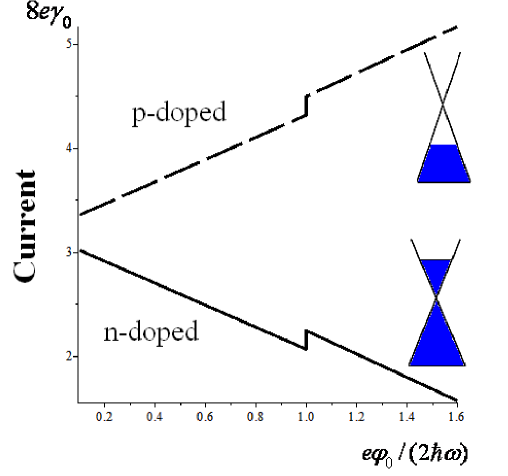
Figure 3: Current in the linear regime for n-doped ($\mu>0$, solid) and p-doped ($\mu<0$, dashed) graphene electrode as a function of applied voltage bias. $|\varepsilon_{m}|=3\hbar\omega$, $\alpha=0.7$.

the steps when the potential of the graphene electrode achieves the value corresponding to the photon energy. The steps are found on the background that decreases linearly for a n-doped graphene electrode and increases linearly for a p-doped electrode when $e\varphi_{0}$ increases. This is related to the linear dependence of DOS on energy. Fig.2 shows our model together with the photonic replica of the graphene electrodes and elucidates the behavior observed in Fig.3.

When the interaction with external field is not small, $\alpha\geq 1$, the linear consideration does not apply. In case of large momenta (far from the Dirac point), $b<<1$, Eq.(48) applies, and we get from Eq.(47) $\left|c_{l}(p,\theta)\right|^{2}=J_{l}^{2}(\alpha\cos\theta)$. The current, Eq.(41), calculated for large momenta when $\alpha=3$, as a function of applied voltage bias is shown in Fig.4. The number of steps and their heights increase in comparison with the linear case.

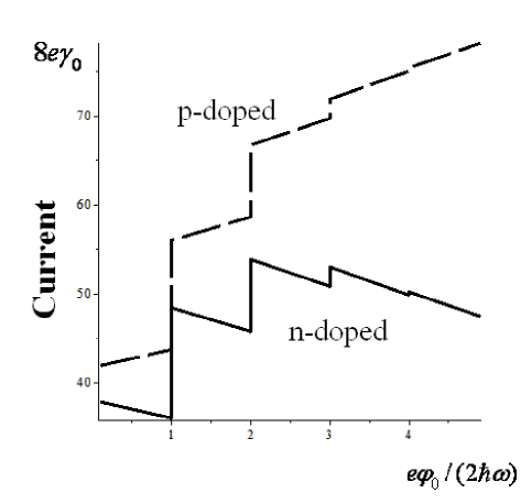
Figure 4: Current in the case of large momenta for n-doped ($\mu>0$, solid) and p-doped ($\mu<0$, dashed) graphene electrode as a function of applied voltage bias. $|\varepsilon_{m}|=20\hbar\omega$, $\alpha=3$.

V.2 Calculations of Current including Small Momenta

To calculate coefficients $c_{l}(p,\theta)$, Eq.(32), in general case, we need to know quasienergy $\varepsilon(p,\theta)$. The latter may be found as zero harmonic of the Fourier cosine series of normal momentum $\bar{p}(t)$ on the left-hand side of Eq.(32). Consider first limiting points $\theta=0,\pi$ when the momentum is parallel to the electric field. Then the quasienergy weighted per the work done by the electric field during one fourth of period is equal to $\bar{\varepsilon}(p;\theta=0,\pi)\equiv\varepsilon(p;\theta=0,\pi)/(evE_{0}/\omega)=[1/(2\pi b)]\int_{-\pi}^{\pi}dx\left|1\pm b\sin x\right|$. If $b<1$, $\bar{\varepsilon}(p;\theta=0,\pi)=1/b\sim vp$ like above. When $b>1$,

$$\bar{\varepsilon}(p;\theta=0,\pi)=\frac{2}{\pi b}[\arcsin(\frac{1}{b})+\sqrt{1-\frac{1}{b^{2}}}]$$ (49)

that gives for $b>>1$

$$\varepsilon(p;\theta=0,\pi)=\frac{1}{\pi}[2\alpha\hbar\omega+\frac{(vp)^{2}}{evE_{0}/\omega}]$$ (50)

- a quadratic dependence of $\varepsilon(p;\theta=0,\pi)$ on $vp$ for small $vp$ or large $evE_{0}/\omega$ accompanied by opening the gap $4\alpha\frac{\hbar\omega}{\pi}$ (see Fig.6 below). This gap is different from those predicted in Refs.Efetov08PRB , Oka_Aoki09PRB , which are induced by interband transitions in an undoped graphene. In contrast, a semiclassical approximation used in our work is correct for doped graphene when $\hbar\omega<2\mu$ Mikhailov07EPL , and as a consequence, interband transitions are excluded. Therefore, in our case the gap is induced by intraband processes. When $\varepsilon(p;\theta=0,\pi)$ is defined by Eq.(50), quantities $\bar{\gamma}_{G_{L}\sigma,m}^{(n)\pm},$ Eq.(35), become $\bar{\gamma}_{G_{L}\sigma,m}^{(n)\pm}=\alpha\gamma_{0}/4$ that do not depend on $n$ and are proportional to $\alpha$.

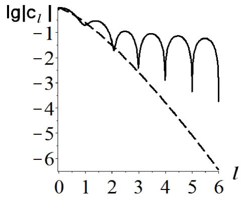
Figure 5: The logarithm of the absolute values of Fourier-coefficients $c_{l}(p;\theta=0,\pi)$ (solid line) versus harmonic number $l$ for n-doped graphene contact ($\mu>0$) and $\alpha=0.5$, $b=1.43>1$. For comparison we also show $|J_{l}(\alpha)|$ (dashed line). We use the continuous variable $l$ though $l$ takes only the whole values.

Fig.5 shows the logarithm of the absolute values of Fourier-coefficients $c_{l}^{+}(p;\theta=0,\pi)$ for different $l$ calculated using Eqs.(32), (36) and (49). For comparison we also show the usual dependence $\left|c_{l}(p;\theta=0,\pi)\right|=|J_{l}(\alpha)|$. One can see much slower falling down $\left|c_{l}^{+}(p;\theta=0,\pi)\right|$ with harmonics index $l$ in comparison to the usual dependence that may be explained by the peculiarities of the graphene spectrum.

One can show that $\left|c_{l}(p,\theta\right|$ falls down as $1/l$ for $b>>1$ and $\alpha<<1$. Indeed, using Eqs.(50) and (55), one can obtain for Fourier-coefficients $c_{l}(p,\theta)$, Eq.(32),

$$c_{l}(p,\theta)=\frac{1}{\pi}\operatorname{Re}{\displaystyle\int\limits_{0}^{\pi}}\exp[i\alpha(\cos\tau-1)+i\tau(l+\frac{2\alpha}{\pi})]d\tau$$ (51)

when $b>>1$ (small momenta). To calculate integral on the right-hand side of Eq.(51), we use expansion, Eq.(46), that gives

$$c_{l}(p,\theta)=\frac{2}{\pi}\sum_{n=-\infty}^{\infty}\frac{J_{n}(\alpha)}{l+\frac{2\alpha}{\pi}+n}\left\{\begin{array}[c]{c}(-1)^{n/2}\sin\alpha\text{, }n\text{ is even}\\ (-1)^{\frac{n+1}{2}+1}\cos\alpha\text{, }n\text{ is odd }\end{array}\right\}$$ (52)

where $l=2k$ is even. If $l=2k+1$, $c_{l}(p,\theta)=0$. Eq.(52) gives $c_{0}(p,\theta)\simeq 1$ and

$$c_{l}(p,\theta)\simeq\frac{2\alpha}{\pi}(\frac{1}{l}+\frac{l}{l^{2}-1}),\text{ }l\geqslant 2$$ (53)

for $\alpha<<1$. Eq.(53) shows that $c_{l}(p,\theta)\sim 1/l$ for $l>2$. Such a behaviour is due to stronly non-linear EM response of graphene, which could also work as a frequency multiplier Mikhailov07EPL . Our approach enables us to understand the origin of this non-linear response that arises due to modification of graphene gapless spectrum in the external EM field.

Consider now the middle point $\theta=\pi/2$ when the momentum is perpendicular to the electric field. In that case one can show that

$$\bar{\varepsilon}(p;\theta =\pi/2)=\frac{1}{2\pi b}\int_{-\pi}^{\pi}dx\sqrt{1+b^{2}\sin^{2}x}=$$

$$=\frac{2}{\pi}\sqrt{1+b^{-2}}E[(1+b^{-2})^{-1/2}]$$ (54)

where $E(x)$ is the complete elliptic integral of the second kind Abr64 . If $b\ll 1$, $\bar{\varepsilon}(p,\pi/2)=1/b$ like before. When $b>>1$, we get

$$\varepsilon(p,\theta=\frac{\pi}{2})=\frac{1}{\pi}\{2\alpha\hbar\omega+[\frac{1}{2}+2\ln(2\sqrt{\frac{eE_{0}}{\omega p}})]\frac{(vp)^{2}}{evE_{0}/\omega}\}$$ (55)

where the dependence of $\varepsilon(p,\pi/2)$ on $p$ for small $p$ (or large $eE_{0}/v)$ differs from quadratic one (cf. with Eq.(50)). Hence, the quasienergy becomes anisotropic, however, its formation is accompanied by opening the same dynamical gap $4\alpha\frac{\hbar\omega}{\pi}$ as for $\theta=0,\pi$. Quasienergies $\bar{\varepsilon}(p;\theta=0,\pi,\pi/2)$ defined by Eqs.(49) and (54) as functions of $1/b=vp/(eE_{0}v/\omega)$ are shown in Fig.6. They are equal to $2/\pi$ for zero momentum, then increase as $\sim(vp)^{2}$ for $\theta=0,\pi$, Eq.(50), and according to Eq.(55) for $\theta=\pi/2$. The law, Eq.(49), for $\theta=0,\pi$ gives way to linear one when $1/b=1$, and quasienergy for $\theta=\pi/2$ also tends to linear one when $1/b>>1$ (large momenta).

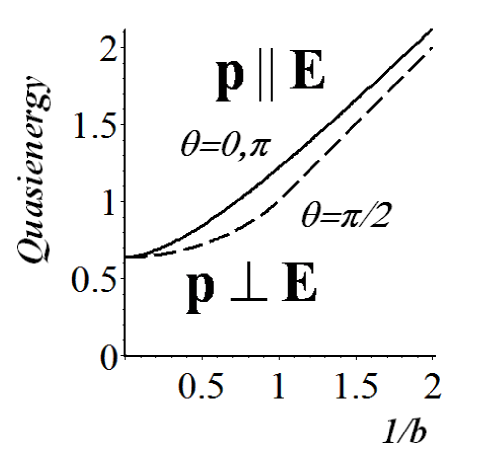
Figure 6: Quasienergies $\bar{\varepsilon}(p;\theta)$ for $\theta=0,\pi$ (solid line) and $\pi/2$ (dashed line) as functions of $1/b=p\omega/(eE_{0})$.

VI Conclusion and Outlook

Here we have proposed and explored theoretically a new approach to coherent control of electric transport via molecular junctions, using graphene electrodes. Our approach is based on the excitation of dressed states of the doped graphene with electric field that is parallel to its surface, having used unique properties of the graphene. We have calculated a semiclassical wave function of a doped graphene under the action of EM excitation and the current through a molecular junction with graphene electrodes using non-equilibrium Green functions. We have shown that using graphene electrodes can essentially enhance currents evaluated at side-band energies $\sim n\hbar\omega$ in molecular nanojunctions that is related to the modification of the graphene gapless spectrum under the action of external EM field. We have calculated the corresponding quasienergy spectrum that is accompanied with opening the gap induced by intraband excitations.

If one shall use an electric field that is perpendicular to the graphene sheet, the field can excite $p$-polarized surface plasmons propagating along the sheet with very high levels of spatial confinement and large near-field enhancement Abajo11NL ; Chen12Nature ; Fei12Nature . Furthermore, surface plasmons in graphene have the advantage of being highly tunable via electrostatic gating Mak08PRL ; Chen8Nature ; Abajo11NL ; Chen12Nature ; Fei12Nature ; Cox12PRB . These plasmon oscillations can enhance the dipole light-matter interaction in a molecular bridge resulting in much more efficient control of photocurrent related to the processes occurring in the molecular bridge under the action of EM field polarized along the bridge Kohler05 ; Kleinekathofer06EPL ; Li07EPL ; Li08SSP ; Fainberg13CPL . By this means a side benifit of using doped graphene electrodes in molecular nanojunctions is the polarization control of the processes occurring either in the graphene electrodes (if the electric field is parallel to the graphene sheet) or in the molecular bridge (if the electric field is perpendicular to the graphene sheet). Such selectivity may be achieved by changing the polarization of an external EM field. This issue will be studied in more detail elsewhere.

References

• (1) S. Kohler, J. Lehmann, and P. Hanggi, Phys. Reports 406, 379 (2005)
• (2) F. Chen and N. J. Tao, Accounts of Chemical Research 42, 429 (2009)
• (3) J. R. Heath, Annual Review of Materials Research 39, 1 (2009)
• (4) T.-H. Park and M. Galperin, Phys. Rev. B 84, 075447 (2011)
• (5) L. Wang and V. May, Phys. Chem. Chem. Phys 13, 8755 (2011)
• (6) B. D. Fainberg, M. Sukharev, T.-H. Park, and M. Galperin, Phys. Rev. B 83, 205425 (2011)
• (7) R. Haertle, R. Volkovich, and M. Thoss, J. Chem. Phys. 133, 081102 (2010)
• (8) M. G. Reuter, M. Sukharev, and T. Seideman, Phys. Rev. Lett. 101, 208303 (2008)
• (9) G. Li, M. Schreiber, and U. Kleinekathoefer, Physica Status Solidi B-Basic Solid State Physics 245, 2720 (2008)
• (10) I. Thanopulos, E. Paspalakis, and V. Yannopapas, Nanotechnology 19, 445202 (2008)
• (11) A. Prociuk and B. D. Dunietz, Phys. Rev. B 78, 165112 (2008)
• (12) G. Li, M. Schreiber, and U. Kleinekathoefer, New J. Phys. 10, 085005 (2008)
• (13) M. Galperin and S. Tretiak, J. Chem. Phys. 128, 124705 (2008)
• (14) U. Kleinekathofer, G. Li, S. Welack, and M. Schreiber, Europhys. Letters 79, 27006 (2007)
• (15) B. D. Fainberg, M. Jouravlev, and A. Nitzan, Phys. Rev. B 76, 245329 (2007)
• (16) G. Platero and R. Aguado, Phys. Reports 395, 1 (2004)
• (17) A. H. L. Dayem and R. J. Martin, Phys. Rev. Lett. 8, 246 (1962)
• (18) P. K. Tien and J. P. Gordon, Phys. Rev. 129, 647 (1963)
• (19) M. Grifoni and P. Hanggi, Phys. Reports 304, 229 (1998)
• (20) U. Kleinekathofer, G. Li, S. Welack, and M. Schreiber, Europhys. Letters 75, 139 (2006)
• (21) A. H. C. Neto, F. Guinea, N. M. R. Peres, K. S. Novoselov, and A. K. Geim, Rev. Mod. Phys. 81, 109 (2009)
• (22) B. Trauzettel, Y. M. Blanter, and A. F. Morpurgo, Phys. Rev. B 75, 035305 (2007)
• (23) S. V. Syzranov, M. V. Fistul, and K. B. Efetov, Phys. Rev. B 78, 045407 (2008)
• (24) X. Zheng, S.-H. Ke, and W. Yang, J. of Chem. Phys 132, 114703 (2010)
• (25) S. A. Mikhailov, Europhys. Letters 79, 27002 (2007)
• (26) B. D. Fainberg and T. Seideman, Chem. Phys. Lett. 576 (2013), [Frontiers Article]
• (27) F. H. L. Koppens, D. E. Chang, and F. J. G. de Abajo, Nano Letters 11, 3370 (2011)
• (28) J. Chen, M. Badioli, P. Alonso-Gonzalez, S. Thongrattanasiri, F. Huth, J. Osmond, M. Spasenovic, A. Centeno, A. Pesquera, P. Godignon, A. Z. Elorza, N. Camara, F. J. G. de Abajo, R. Hillenbrand, and F. H. L. Koppens, Nature 487, 77 (2012)
• (29) Z. Fei, A. S. Rodin, G. O. Andreev, W. Bao, A. S. McLeod, M. Wagner, L. M. Zhang, Z. Zhao, M. Thiemens, G. Dominguez, M. M. Fogler, A. H. C. Neto, C. N. Lau, F. Keilmann, and D. N. Basov, Nature 487, 82 (2012)
• (30) K. F. Mak, M. Y. Sfeir, Y. Wu, C. H. Lui, J. A. Misewich, and T. F. Heinz, Phys. Rev. Lett. 101, 196405 (2008)
• (31) C.-F. Chen, C.-H. Park, B. W. Boudouris, J. Horng, B. Geng, C. Girit, A. Zettl, M. F. Crommie, R. A. Segalman, S. G. Louie, and F. Wang, Nature 471, 617 (2011)
• (32) W. Pauli, Helv. Phys. Acta 5, 179 (1932)
• (33) A. I. Akhiezer and V. B. Berestetskii, Quantum electrodynamics (Nauka, Moskow, 1969) in Russian
• (34) V. B. Berestetskii, E. M. Lifshitz, and L. P. Pitaevskii, Quantum electrodynamics (Butterworth-Heinemann, Oxford, 1999)
• (35) L. D. Landau and E. M. Lifshitz, Quantum mechanics non-relativistic theory (Pergamon Press, New York, 1965)
• (36) H. Haug and A. P. Jauho, Quantum Kinetics in Transportand Optics of Semiconductors (Springer, Berlin, 1996)
• (37) M. Abramowitz and I. Stegun, Handbook on Mathematical Functions (Dover, New York, 1964)
• (38) G. Li, M. S. Shishodia, B. D. Fainberg, B. Apter, M. Oren, A. Nitzan, and M. Ratner, Nano Letters 12, 2228 (2012)
• (39) T. Oka and H. Aoki, Phys. Rev. B 79, 081406 (2009)
• (40) J. D. Cox, M. R. Singh, G. Gumbs, M. A. Anton, and F. Carreno, Phys. Rev. B 86, 125452 (2012)