Long-time Behavior of Random Walks in Random Environment

Abstract

We study behavior in space and time of random walks in an i.i.d. random environment on $\mathbb{Z}^{d}$, $d\geq 3$. It is assumed that the measure governing the environment is isotropic and concentrated on environments that are small perturbations of the fixed environment corresponding to simple random walk. We develop a revised and extended version of the paper of Bolthausen and Zeitouni (2007) on exit laws from large balls, which, as we hope, is easier to follow. Further, we study mean sojourn times in balls.

This work is part of the author’s PhD thesis under the supervision of Erwin Bolthausen. A generalization of the results on exit measures to certain anisotropic random walks in random environment is available at arXiv:1309.3169 [math.PR].

Subject classifications: 60K37; 82C41.
Key words: random walk, random environment, exit measure, pertubative regime, non-ballistic behavior, isotropic.

0 Introduction

0.1 The model

General description

Consider the integer lattice $\mathbb{Z}^{d}$ with unit vectors $e_{i}$, whose $i$th component equals $1$. We let $\mathcal{P}$ be the set of probability distributions on $\{\pm e_{i}:i=1,\ldots,d\}$. Given a probability measure $\mu$ on $\mathcal{P}$, we equip $\Omega=\mathcal{P}^{\mathbb{Z}^{d}}$ with its natural product $\sigma$-field $\mathcal{F}$ and the product measure $\mathbb{P}_{\mu}=\mu^{\otimes\mathbb{Z}^{d}}$. Each element $\omega\in\Omega$ yields transition probabilities of a nearest neighbor Markov chain on $\mathbb{Z}^{d}$, the random walk in random environment (RWRE for short), via

$$p_{\omega}(x,x+e)=\omega_{x}(e),\quad e\in\{\pm e_{i}:i=1,\ldots,d\}.$$

We write $\operatorname{P}_{x,\omega}$ for the “quenched” law of the canonical Markov chain $(X_{n})_{n\geq 0}$ with these transition probabilities, starting at $x\in\mathbb{Z}^{d}$. The probability measure

$$P=\int_{\Omega}\operatorname{P}_{0,\omega}\mathbb{P}(\textup{d}\omega)$$

is commonly referred to as averaged or “annealed” law of the RWRE started at the origin.

Additional requirements

We study asymptotic properties of the RWRE in dimension $d\geq 3$ when the underlying environments are small perturbations of the fixed environment $\omega_{x}(\pm e_{i})=1/(2d)$ corresponding to simple or standard random walk. In order to fix a perturbative regime, we introduce the following condition.

• Let $0<\varepsilon<1/(2d)$. We say that $\operatorname{\bf{A0}}(\varepsilon)$ holds if $\mu(\mathcal{P}_{\varepsilon})=1$, where

  $$\mathcal{P}_{\varepsilon}=\left\{q\in\mathcal{P}:\left|q(\pm e_{i})-1/(2d)\right|\leq\varepsilon\mbox{ for all }i=1,\ldots,d\right\}.$$

The perturbative behavior concerns the behavior of the RWRE when $\operatorname{\bf{A0}}(\varepsilon)$ holds for small $\varepsilon$. However, even for arbitrarily small $\varepsilon$, such walks can behave very differently compared to simple random walk. This motivates a further “centering” restriction on $\mu$.

• We say that $\operatorname{\bf{A1}}$ holds if $\mu$ is invariant under all orthogonal transformations fixing the lattice $\mathbb{Z}^{d}$, i.e. if $O:\mathbb{R}^{d}\rightarrow\mathbb{R}^{d}$ is any orthogonal matrix that maps $\mathbb{Z}^{d}$ onto itself, then the laws of $(\omega_{0}(Oe))_{|e|=1}$ and $(\omega_{0}(e))_{|e|=1}$ coincide.

If $\operatorname{\bf{A1}}$ holds, $\mathbb{P}_{\mu}$ is called isotropic.

0.2 Informal description of the results

In the following, we write $\mathbb{P}$ instead of $\mathbb{P}_{\mu}$ and denote by $\mathbb{E}$ the corresponding expectation.

Exit laws from balls

In the main part of this work, we investigate the RWRE exit distribution from the ball $V_{L}=\{x\in\mathbb{Z}^{d}:|x|\leq L\}$ when the radius $L$ is large. Assuming $\operatorname{\bf{A1}}$ and $\operatorname{\bf{A0}}(\varepsilon)$ for small $\varepsilon$, we show that the exit law of the walk, started from a point $x$ with $|x|\leq L/5$, is close to that of simple random walk. More precisely, using the multiscale analysis introduced in Bolthausen and Zeitouni [6], we prove that if the radius $L$ tends to infinity, then

1. The difference of the two exit laws measured in total variation stays small as $L$ increases (but does not tend to zero, due to boundary effects) (Theorem 1.1 (i)).

2. The distance between the two exit laws converges to zero if they are convolved with an additional smoothing kernel on a scale increasing arbitrarily slowly with $L$ (Theorem 1.1 (ii)).

3. The RWRE exit measure of boundary portions of size $\geq(L/(\log L)^{15})^{d-1}$ can be bounded from above by that of simple random walk. Evaluated on segments of size $\geq(L/(\log L)^{6})^{d-1}$, the two measures agree up to a multiplicative error, which tends to one as $L$ increases (Theorem 1.2).

The first two parts already appeared in [6], which serves as the basis for our work. However, for reasons explained below, it was of great interest to find a somewhat different approach.

Mean sojourn times

The results on exit laws can be used to prove transience of the RWRE (Corollary 1.1), and they provide an invariance principle up to time transformation. Getting complete control over time is a major open problem, and in that direction, we look in Section 8 at mean holding or sojourn times in balls. Our basic insight is that exceptionally small or large times can only be produced by spatially atypical regions. Consequently, the philosophy behind our approach is to derive statements on sojourn times from estimates on exit laws. However, our results on exit distributions seem not quite sufficient to handle the presence of strong traps, i.e. regions where the RWRE cannot escape for a long time with high probability. We therefore make an additional assumption which guarantees that the mass of environments producing very large times is sufficiently small. Let $\tau_{L}=\inf\{n\geq 0:X_{n}\notin V_{L}\}$ be the first exit time of the RWRE from the ball $V_{L}$, and denote by $\operatorname{E}_{0,\omega}$ the expectation with respect to $\operatorname{P}_{0,\omega}$.

• We say that A2 holds if for large $L$,

  $$\mathbb{P}\left(\operatorname{E}_{0,\omega}\left[\tau_{L}\right]>(\log L)^{4}L^{2}\right)\leq L^{-8d}.$$

Assuming this additional condition, we prove

1. For almost all environments, the normalized quenched mean time $\operatorname{E}_{0,\omega}[\tau_{L}]/L^{2}$ is finally contained in a small interval around one, where the size of the interval converges to zero if the disorder $\varepsilon$ tends to zero (Proposition 1.2 and Theorem 1.3).

We believe that A2 follows from $\operatorname{\bf{A0}}(\varepsilon)$ and $\operatorname{\bf{A1}}$, even with a faster decay of the probability. It remains an open (and possibly challenging) problem to prove this. An example where A2 trivially holds true is given in Remark 8.1.

0.3 Discussion of this work

The part on exit measures should be seen as a corrected and extended version of Bolthausen and Zeitouni [6]. Most of the ideas can already be found there, and also our proofs sometimes follow those of [6]. However, our focus lies more on Green’s function estimates on “goodified” environments, which are developed in Section 4. Partly based on (unpublished) notes of Bolthausen, this section is entirely new, and the results obtained make the proofs of the main statements more transparent. The core statement is Lemma 4.1, which gives a bound on the (coarse grained) RWRE Green’s function, for a large class of environments. As such estimates were only partially present in [6], the authors had to repeatedly consider higher order expansions in terms of Green’s functions coming from simple random walk, which led to serious problems, for example in Sections 4.3 and 4.4 in [6].

The reason for developing a new approach was twofold: On the one hand, it seemed difficult to fix these problems ad hoc. On the other hand, we aimed at establishing a solid basis for future work on this topic, in particular in the direction of a central limit theorem. Further new points of this work can be summarized as follows.

• We give either new proofs of the statements in [6] or we revise the old ones. For example, the proofs leading to the main results on the exit measures in Sections 5 and 6 are based on our new techniques. These include the bounds on Green’s functions, the use of parametrized coarse graining schemes and the concept of goodified environments, which goes back to [6] and is further elaborated here.

• The appendix is completely rewritten. In this part, the main corrections concern the proof of the key Lemma 3.2 (Lemma 3.4 in [6]), where different case had to be considered. Also, we provide a lower bound on exit probabilities (Lemma 3.2 (iii)), which was already implicitly used in [6], but not proved.

• We obtain local estimates for the exit measures (Theorem 1.2). The global estimates in total variation distance are extended to starting points $|x|\leq L/5$.

• The results on the exit distributions are used to control the mean sojourn time of the RWRE in balls, under an extra assumption on $\mathbb{P}$.

To improve readability, we overview the main steps of this work in Section 1.5.

0.4 A brief history

The literature on random walks in random environment is vast, and we do by no means intend to give a full overview here. Instead, we point at some cornerstones and focus on results which are relevant for our particular model. For a more detailed survey, the reader is invited to consult the lecture notes of Sznitman [30], [32] and Zeitouni [38], [39], and also the overview article of Bogachev [7].

Recall the general model defined at the very beginning under “General description”. We additionally assume that the environment is uniformly elliptic, i.e. there exists $\kappa>0$ such that $\mathbb{P}$-almost surely, $\omega_{x}(e)\geq\kappa$ for all $x,e\in\mathbb{Z}^{d}$, $|e|=1$. Note that in the perturbative regime, this is automatically true.

The natural condition of uniform ellipticity can sometimes be relaxed to mere ellipticity $\omega_{x}(e)>0$ for $x,e\in\mathbb{Z}^{d}$, $|e|=1$. Also, it often suffices to require $\mathbb{P}$ to be stationary and ergodic instead of being “i.i.d.”.

Dimension $d=1$

Early interest in models of RWRE can be traced back to the 60’s in the context of biochemistry, where they were used as a toy model for DNA replication, cf. Chernov [9] and Temkin [35]. Solomon [27] started a rigorous mathematical analysis in dimension $d=1$. He proved that if

$$\mathbb{E}\left[\log\rho\right]\neq 0,\quad\mbox{where }\rho=\omega_{0}(-1)/\omega_{0}(1),$$

then the RWRE is $P$-almost surely transient, whereas in the case $\mathbb{E}\left[\log\rho\right]=0$, the walk is $P$-a.s. recurrent. Further, he obtained almost sure existence of the limit speed $v=\lim_{n\rightarrow\infty}X_{n}/n$,

$$v=\left\{\begin{array}[]{l@{\quad}l}\frac{1-\mathbb{E}[\rho]}{1+\mathbb{E}[\rho]}&\mbox{if\ }\mathbb{E}[\rho]<1\\ \frac{1-\mathbb{E}[\rho^{-1}]}{1+\mathbb{E}[\rho^{-1}]}&\mbox{if\ }\mathbb{E}[\rho^{-1}]<1\\ 0&\mbox{otherwise}\end{array}\right..$$

His results already reveal some surprising features of the model. For example, it can happen that $v=0$, but nonetheless the RWRE is transient (note that this is impossible for a Markov chain with stationary increments, according to Kesten [18]). Also, if $\overline{v}=\mathbb{E}[\omega_{0}(1)-\omega_{0}(-1)]$ denotes the mean local drift, it is possible that $|v|<|\overline{v}|$. Such slowdown effects, caused by traps reflecting impurities in the medium, come again to light in limit theorems for the RWRE under both the quenched and the annealed measure. In [20], Kesten, Kozlov and Spitzer proved that in the transient case under the annealed law, both diffusive and sub-diffusive behavior can occur, depending on a critical exponent connected to hitting times. However, the strongest form of sub-diffusivity appears in the recurrent case with non-degenerate site distribution $\mu$, for which Sinai [26] proved that after $n$ steps, the RWRE is typically at distance of order only $(\log n)^{2}$ away from the starting point. His analysis shows that the walk spends most of the time at the bottom of certain valleys. The limit law of $X_{n}/(\log n)^{2}$ is given by the distribution of a functional of Brownian motion, cf. Kesten [19] and Golosov [14]. Let us finally mention that slowdown phenomena also show up when studying probabilities of atypical events like large deviations, see e.g. [15], [11], [13].

Dimensions $d\geq 2$

While the one-dimensional picture is quite complete, many questions remain open in higher dimensions, including a classification into recurrent/transient behavior, existence of a limit speed and invariance principles. The main difficulties come from the non-Markovian character under the annealed measure and the fact that the RWRE is irreversible under the quenched measure as soon as $d\geq 2$.

Let us illustrate one prominent open problem, the directional zero-one law. For an element $l$ from the unit sphere $\mathbb{S}^{d-1}$, denote the event that the RWRE is transient in direction $l$ by

$$A_{l}=\left\{\lim_{n\rightarrow\infty}X_{n}\cdot l=\infty\right\}.$$

Kalikow proved in [17] that $P(A_{l}\cup A_{-l})\in\{0,1\}$. Is it also true that $P(A_{l})\in\{0,1\}$ ? The answer is affirmative in dimension $d=1,2$ ([27] for $d=1$, Merkl and Zerner [25] for $d=2$), but unknown for higher dimensions. It is known that a limit speed $v\in\mathbb{R}^{d}$ (possibly zero) exists if $P(A_{l})\in\{0,1\}$ for every $l\in\mathbb{S}^{d-1}$, cf. Sznitman and Zerner [34].

Much progress has been made in characterizing models which exhibit ballistic behavior, that is when the limit velocity $v$ is an almost sure constant vector different from zero. Here Sznitman’s conditions $(T_{\gamma})$, $\gamma\in(0,1]$, give a criterion for ballisticity and lead to an invariance principle under the annealed measure $P$, see Sznitman [28], [29] and also his lecture notes [32]. When $d\geq 4$ and the disorder is small, a quenched invariance principle has been shown by Bolthausen and Sznitman [4]. A stronger ballisticity condition was given earlier by Kalikow [17]. However, as examples in Sznitman [31] demonstrate, Kalikow’s condition does not completely describe ballistic behavior in dimensions $d\geq 3$. A handy and complete characterization of ballisticity has still to be found. For recent developments, see the work of Berger [1] and Berger, Drewitz, Ramírez [2]. In [2], it is conjectured that in dimensions $d\geq 2$, a RWRE which is transient in all directions $l$ out of an open subset $U\subset\mathbb{S}^{d-1}$ is ballistic (for an i.i.d uniformly elliptic environment).

Turning to ballistic behavior in the perturbative regime, Sznitman shows in [31] that for $0<\eta<5/2$ in dimension $d=3$ or for $0<\eta<3$ in dimensions $d\geq 4$, there exists $\varepsilon_{0}=\varepsilon_{0}(d,\eta)$ such that if $\operatorname{\bf{A0}}(\varepsilon)$ is fulfilled for some $\varepsilon\leq\varepsilon_{0}$ and the mean local drift under the static measure satisfies

$$\mathbb{E}[d(0,\omega)\cdot e_{1}]>\left\{\begin{array}[]{l@{\quad}l}\varepsilon^{5/2-\eta}&\mbox{if }d=3\\ \varepsilon^{3-\eta}&\mbox{if }d\geq 4\end{array},\right.\quad\mbox{where }d(0,\omega)=\sum_{|e|=1}e\omega_{0}(e),$$

then the RWRE is ballistic in direction $e_{1}$, i.e. $v\cdot e_{1}\neq 0$. Moreover, a functional limit theorem holds under $P$. In [5], Bolthausen, Sznitman and Zeitouni consider RWRE in dimensions $d\geq 6$ where the projection onto at least five components behaves as simple random walk. Among other things, examples are constructed under $\operatorname{\bf{A0}}(\varepsilon)$ for which $\mathbb{E}[d(0,\omega)]\neq 0$, but $v=0$ $(d\geq 7)$, and a quenched invariance principle is proved when $d\geq 15$. On the other hand, it can happen that $\mathbb{E}[d(0,\omega)]=0$ but $v\neq 0$. As a further remarkable result of [5], it can even happen that $0\neq v=-c\mathbb{E}[d(0,\omega)]$ for some $c>0$, which exemplifies that the environment acts on the path of the walk in a highly nontrivial way. Large deviations of $X_{n}/n$ are studied in Varadhan [36].

Concerning non-ballistic behavior, much is known for the class of balanced RWRE when $\mathbb{P}(\omega_{0}(e_{i})=\omega_{0}(-e_{i}))=1$ for all $i=1,\ldots,d$. One first notices that the walk is a martingale, which readily leads to limit speed zero. Employing the method of environment viewed from the particle, Lawler proves in [22] that for $\mathbb{P}$-almost all $\omega$, $X_{\lfloor n\cdot\rfloor}/\sqrt{n}$ converges in $\operatorname{P}_{0,\omega}$-distribution to a non-degenerate Brownian motion with diagonal covariance matrix. Moreover, the RWRE is recurrent in dimension $d=2$ and transient when $d\geq 3$, see [38]. Recently, within the i.i.d. setting, diffusive behavior has been shown in the mere elliptic case by Guo and Zeitouni [16] and in the non-elliptic case by Berger and Deuschel [3].

Our study of random walks in random environment in the perturbative regime under the isotropy condition $\operatorname{\bf{A1}}$ aims at a quenched central limit theorem, showing that in dimensions $d\geq 3$, the RWRE is asymptotically Gaussian, on $\mathbb{P}$-almost all environments $\omega$. Such an invariance principle has already been shown by Bricmont and Kupiainen [8], who introduced condition $\operatorname{\bf{A1}}$. However, it is of interest to find a self-contained new proof. A continuous counterpart of this model, isotropic diffusions in a random environment which are small perturbations of Brownian motion, has been investigated by Sznitman and Zeitouni in [33]. They prove transience and a full quenched invariance principle in dimensions $d\geq 3$.

0.5 Open problems for our model and ongoing work

As we already pointed out above, with respect to a central limit theorem one still needs to find ways to handle large times, which are in a certain sense excluded by Assumption A2. In this direction, a more complete picture of exit laws could prove helpful, including sharper estimates for the appearance of balls with an atypical exit measure. A further task is to combine space and time estimates in the right way.

In the direction of a fully perturbative theory it would be desirable to replace the isometry condition $\operatorname{\bf{A1}}$ by the requirement that $\mu$ is just invariant under reflections mapping a unit vector to its inverse. Then the RWRE exit law from a ball should be close to that of some $d$-dimensional symmetric random walk. The relaxed condition on $\mu$ would, for example, include the class of walks that are balanced in one coordinate direction, where time can be controlled much easier. This is work in progress.

Another open problem is the case of small isotropic perturbations in dimension $d=2$. One expects diffusive behavior as in dimensions $d\geq 3$, but there is no rigorous result yet. In principle, one might try to follow a similar multiscale approach for the exit measures as it is presented below. But the same perturbation argument shows that unlike dimensions $d\geq 3$, the disorder does not contract in leading order. Therefore, one has to look closer at higher order terms. While for $d\geq 3$, the nonlinear terms in the perturbation expansion for the Green’s function can be estimated in a somewhat crude way once the right scales are found, it seems that in dimension $d=2$, at least terms up to order three have to be carefully taken into account.

1 Basic notation and main results

1.1 Basic notation

Our purpose here is to cover the most relevant notation which will be used throughout this text. Further notation will be introduced later on when needed.

Sets and distances

We have $\mathbb{N}=\{0,1,2,3,\ldots\}$ and $\mathbb{R}_{+}=\{x\in\mathbb{R}:x\geq 0\}$. For a set $A$, its complement is denoted by $A^{c}$. If $A\subset\mathbb{R}^{d}$ is measurable and non-discrete, we write $|A|$ for its $d$-dimensional Lebesgue measure. Sometimes, $|A|$ denotes the surface measure instead, but this will be clear from the context. If $A\subset\mathbb{Z}^{d}$, then $|A|$ denotes its cardinality.

For $x\in\mathbb{R}^{d}$, $|x|$ is the Euclidean norm. If $A,B\subset\mathbb{R}^{d}$, we set $\operatorname{d}(A,B)=\inf\{|x-y|:x\in A,\;y\in B\}$ and $\operatorname{diam}(A)=\sup\{|x-y|:x,y\in A\}$. Given $L>0$, let $V_{L}=\{x\in\mathbb{Z}^{d}:|x|\leq L\}$, and for $x\in\mathbb{Z}^{d}$, $V_{L}(x)=V_{L}+x$. For Euclidean balls in $\mathbb{R}^{d}$ we write $C_{L}=\{x\in\mathbb{R}^{d}:|x|<L\}$ and for $x\in\mathbb{R}^{d}$, $C_{L}(x)=x+C_{L}$.

If $V\subset\mathbb{Z}^{d}$, then $\partial V=\{x\in V^{c}\cap\mathbb{Z}^{d}:\operatorname{d}(\{x\},V)=1\}$ is the outer boundary, while in the case of a non-discrete set $V\subset\mathbb{R}^{d}$, $\partial V$ stands for the usual topological boundary of $V$ and $\overline{V}$ for its closure. For $x\in\overline{C}_{L}$, we set $\operatorname{d}_{L}(x)=L-|x|$. Finally, for $0\leq a<b\leq L$, the “shell” is defined by

$$\operatorname{Sh}_{L}(a,b)=\{x\in V_{L}:a\leq\operatorname{d}_{L}(x)<b\},\ \ \operatorname{Sh}_{L}(b)=\operatorname{Sh}_{L}(0,b).$$

Functions

If $a,b$ are two real numbers, we set $a\wedge b=\min\{a,b\}$, $a\vee b=\max\{a,b\}$. The largest integer not greater than $a$ is denoted by $\lfloor a\rfloor$. As usual, set $1/0=\infty$. For us, $\log$ is the logarithm to the base $e$. For $x,z\in\mathbb{R}^{d}$, the Delta function $\delta_{x}(z)$ is defined to be equals one for $z=x$ and zero otherwise. If $V\subset\mathbb{Z}^{d}$ is a set, then $\delta_{V}$ is the probability distribution on the subsets of $\mathbb{Z}^{d}$ satisfying $\delta_{V}(V^{\prime})=1$ if $V^{\prime}=V$ and zero otherwise.

Given two functions $F,G:\mathbb{Z}^{d}\times\mathbb{Z}^{d}\rightarrow\mathbb{R}$, we write $FG$ for the (matrix) product $FG(x,y)=\sum_{u\in\mathbb{Z}^{d}}F(x,u)G(u,y)$, provided the right hand side is absolutely summable. $F^{k}$ is the $k$th power defined in this way, and $F^{0}(x,y)=\delta_{x}(y)$. $F$ can also operate on functions $f:\mathbb{Z}^{d}\rightarrow\mathbb{R}$ from the left via $Ff(x)=\sum_{y\in\mathbb{Z}^{d}}F(x,y)f(y)$.

We use the symbol $1_{W}$ for the indicator function of the set $W$. By an abuse of notation, $1_{W}$ will also denote the kernel $(x,y)\mapsto 1_{W}(x)\delta_{x}(y)$. If $f:\mathbb{Z}^{d}\rightarrow\mathbb{R}$, $||f||_{1}=\sum_{x\in\mathbb{Z}^{d}}|f(x)|\in[0,\infty]$ is its $L^{1}$-norm. When $\nu:\mathbb{Z}^{d}\rightarrow\mathbb{R}$ is a (signed) measure, $||\nu||_{1}$ is its total variation norm.

Let $U\subset\mathbb{R}^{d}$ be a bounded open set, and let $k\in\mathbb{N}$. For a $k$-times continuously differentiable function $f:U\rightarrow\mathbb{R}$, that is $f\in C^{k}(U)$, we define for $i=0,1,\ldots,k$,

$${\left|\left|D^{i}f\right|\right|}_{U}=\sup_{|\beta|=i}\sup_{U}\left|\frac{\partial^{i}}{\partial x_{1}^{\beta_{1}}\cdots\partial x_{d}^{\beta_{d}}}f\right|,$$

where the first supremum is over all multi-indices $\beta=(\beta_{1},\ldots,\beta_{d})$, $\beta_{j}\in\mathbb{N}$, with $|\beta|=\sum_{j=1}^{d}\beta_{j}$. Let $L>0$. Putting $U_{L}=\left\{x\in\mathbb{R}^{d}:L/2<|x|<2L\right\}$, we define

$$\mathcal{M}_{L}=\left\{\psi:U_{L}\rightarrow(L/10,5L),\ \psi\in C^{4}(U_{L}),{\left|\left|D^{i}\psi\right|\right|}_{U_{L}}\leq 10\;\mbox{ for }i=1,\ldots,4\right\}.$$

We will mostly interpret functions $\psi\in\mathcal{M}_{L}$ as maps from $U_{L}\cap\mathbb{Z}^{d}\subset\mathbb{R}^{d}$. A typical function we have in mind is the constant function $\psi\equiv L$.

Transition probabilities and exit distributions

Given (not necessarily nearest neighbor) transition probabilities $p={(p(x,y))}_{x,y\in\mathbb{Z}^{d}}$, we write $\operatorname{P}_{x,p}$ for the law of the canonical Markov chain ${(X_{n})}_{n\geq 0}$ on $({(\mathbb{Z}^{d})}^{\mathbb{N}},\mathcal{G})$, $\mathcal{G}$ the $\sigma$-algebra generated by cylinder functions, with transition probabilities $p$ and starting point $X_{0}=x$  $\operatorname{P}_{x,p}$ -a.s. The expectation with respect to $\operatorname{P}_{x,p}$ is denoted by $\operatorname{E}_{x,p}$. We will often consider the simple random walk kernel $p^{\mbox{\scriptsize RW}}(x,x\pm e_{i})=1/(2d)$.

If $V\subset\mathbb{Z}^{d}$, we denote by $\tau_{V}=\inf\{n\geq 0:X_{n}\notin V\}$ the first exit time from $V$, with $\inf\emptyset=\infty$, whereas $T_{V}=\tau_{V^{c}}$ is the first hitting time of $V$. Given $x,z\in\mathbb{Z}^{d}$ and $p,V$ as above, we define

$$\mbox{ex}_{V}(x,z;\,p)=\operatorname{P}_{x,p}\left(\tau_{V}=z\right).$$

Notice that for $x\in V^{c}$, $\mbox{ex}_{V}(x,z;p)=\delta_{x}(z)$. For simple random walk, we write

$$\pi_{V}(x,z)=\mbox{ex}_{V}\left(x,z;p^{\mbox{\scriptsize RW}}\right).$$

Given $\omega\in\Omega$, we set

$$\Pi_{V}(x,z)=\mbox{ex}_{V}(x,z;p_{\omega}).$$

Here, $\Pi_{V}$ should be understood as a random exit distribution, but we suppress $\omega$ in the notation.

Coarse grained random walks

In order to transfer information about both exit measures and sojourn times from one scale to the next, we work with coarse graining schemes.

Fix once for all a probability density $\varphi\in C^{\infty}(\mathbb{R}_{+},\mathbb{R}_{+})$ with compact support in $(1,2)$. Given a nonempty subset $W\subset\mathbb{Z}^{d}$, $x\in W$ and $m_{x}>0$, the image measure of the rescaled density $(1/m_{x})\varphi(t/m_{x})\textup{d}t$ under the mapping $t\mapsto V_{t}(x)\cap W$ defines a probability distribution on (finite) sets containing $x$. If $\psi=(m_{x})_{x\in W}$ is a field of positive numbers, we obtain in this way a collection of probability distributions indexed by $x\in W$, a coarse graining scheme on $W$.

Now if $p=(p(x,y))_{x\in W,y\in\mathbb{Z}^{d}}$ is a collection of transition probabilities on $W$, we define the coarse grained transitions belonging to $(\psi,\,p)$ by

$$p_{\psi}^{\mbox{\scriptsize CG}}(x,\cdot)=\frac{1}{m_{x}}\int_{\mathbb{R}_{+}}\varphi\left(\frac{t}{m_{x}}\right)\mbox{ex}_{V_{t}(x)\cap W}(x,\cdot;p)\textup{d}t,\quad x\in W.$$ (1)

If $p=p^{\mbox{\scriptsize RW}}$, we write $\hat{\pi}_{\psi}$ instead of $p_{\psi}^{\mbox{\scriptsize CG}}$. Note that for every choice of $W$ and $\psi$, $\hat{\pi}_{\psi}$ defines a probability kernel.

For the motion in the ball $V_{L}$, we use a particular field $\psi$, which we describe in Section 2.1. There, we will also introduce a coarse grained RWRE transition kernel.

Further notation and abbreviations

For simplicity, we set $\operatorname{P}_{x}=\operatorname{P}_{x,p^{\mbox{\tiny RW}}}$, $\operatorname{E}_{x}=\operatorname{E}_{x,p^{\mbox{\tiny RW}}}$. Given transition probabilities $p_{\omega}$ coming from an environment $\omega$, we use the notation $\operatorname{P}_{x,\omega}$, $\operatorname{E}_{x,\omega}$. In order to avoid double indices, we usually write $\pi_{L}$ instead of $\pi_{V}$, $\Pi_{L}$ for $\Pi_{V}$ and $\tau_{L}$ for $\tau_{V}$ if $V=V_{L}$ is the ball of radius $L$ around zero.

Many of our quantities will be indexed by both $L$ and $r$, where $r$ is an additional parameter. While we always keep the indices in the statements, we normally drop both of them in the proofs. We will often use the abbreviations $\operatorname{d}(y,B)$ for $\operatorname{d}(\{y\},B)$, $T_{x}$ for $T_{\{x\}}$ and $\mathbb{P}\left(A;\,B\right)$ for $\mathbb{P}\left(A\cap B\right)$.

Some words about constants, $O$-notation and large $L$ behavior

All our constants are positive. They only depend on the dimension $d\geq 3$ unless stated otherwise. In particular, they do not depend on $L$, on $\omega$ or on any point $x\in\mathbb{Z}^{d}$, and they are also independent of the parameter $r$ which will be introduced in Section 2.

We use $C$ and $c$ for generic positive constants whose values can change in different expressions, even in the same line. If we use other constants like $K,C_{1},c_{1}$, their values are fixed throughout the proofs. Lower-case constants usually indicate small (positive) values.

Given two functions $f,g$ defined on some subset of $\mathbb{R}$, we write $f(t)=O\left(g(t)\right)$ if there exists a positive $C>0$ and a real number $t_{0}$ such that $|f(t)|\leq C|g(t)|\mbox{ for }t\geq t_{0}.$

If a statement holds for “$L$ large (enough)”, this means that there exists $L_{0}>0$ depending only on the dimension such that the statement is true for all $L\geq L_{0}$. This applies analogously to the expressions “$\delta$ (or $\varepsilon$) small (enough)”.

The reader should always keep in mind that we are interested in asymptotics when $L\rightarrow\infty$ and $\varepsilon$ is a (arbitrarily) small positive constant. Even though some of our statements are valid only for large $L$ and $\varepsilon$ sufficiently small, we do not mention this every time.

1.2 Main results on exit laws

We still need some notation. For $x\in\mathbb{Z}^{d}$, $t>0$ and $\psi:\partial V_{t}(x)\rightarrow(0,\infty)$ define

$$D_{t,\psi}(x)=\left|\left|\left(\Pi_{V_{t}(x)}-\pi_{V_{t}(x)}\right)\hat{\pi}_{\psi}(x,\cdot)\right|\right|_{1},$$

$$D_{t}(x)=\left|\left|\left(\Pi_{V_{t}(x)}-\pi_{V_{t}(x)}\right)(x,\cdot)\right|\right|_{1}.$$

If $\psi\equiv m$ is constant, we write $D_{t,m}$ instead of $D_{t,\psi}$. We usually drop $x$ from the notation if $x=0$. Further, let

$$D_{t,\psi}^{\ast}=\sup_{x\in V_{t/5}}\left|\left|\left(\Pi_{V_{t}}-\pi_{V_{t}}\right)\hat{\pi}_{\psi}(x,\cdot)\right|\right|_{1},$$

$$D_{t}^{\ast}=\sup_{x\in V_{t/5}}\left|\left|\left(\Pi_{V_{t}}-\pi_{V_{t}}\right)(x,\cdot)\right|\right|_{1}.$$

With $\delta>0$, we set for $i=1,2,3$

$$b_{i}(L,\psi,\delta)=\mathbb{P}\left(\left\{(\log L)^{-9+9(i-1)/4}<D_{L,\psi}^{\ast}\leq(\log L)^{-9+9i/4}\right\}\cap\left\{D_{L}^{\ast}\leq\delta\right\}\right),$$

and

$$b_{4}(L,\psi,\delta)=\mathbb{P}\left(\left\{D_{L,\psi}^{\ast}>(\log L)^{-3+3/4}\right\}\cup\left\{D_{L}^{\ast}>\delta\right\}\right).$$

The following technical condition will play a key role.

Let $\delta>0$ and $L_{1}\geq 3$. We say that $\operatorname{\bf{C1}}(\delta,L_{1})$ holds if for all $3\leq L\leq L_{1}$, all $\psi\in\mathcal{M}_{L}$, $i=1,2,3,4$,

$$b_{i}(L,\psi,\delta)\leq\frac{1}{4}\exp\left(-\left((3+i)/4\right)(\log L)^{2}\right).$$

Notice that if $\operatorname{\bf{C1}}(\delta,L_{1})$ is satisfied, then for any $3\leq L\leq L_{1}$ and any $\psi\in\mathcal{M}_{L}$,

$$\mathbb{P}\left(\left\{D_{L,\psi}^{\ast}>(\log L)^{-9}\right\}\cup\left\{D_{L}^{\ast}>\delta\right\}\right)\leq\exp\left(-(\log L)^{2}\right).$$

We can now formulate our results. Proposition 1.1, Theorem 1.1 and Corollary 1.1 are in a similar form already present in [6]. See also our discussion in the introduction.

The main technical statement is

Proposition 1.1.

Assume $\operatorname{\bf{A1}}$. There exists $\delta_{0}>0$ such that for any $\delta\in(0,\delta_{0}]$, there exists $\varepsilon_{0}=\varepsilon_{0}(\delta)>0$ with the following property: If $\varepsilon\leq\varepsilon_{0}$ and $\operatorname{\bf{A0}}(\varepsilon)$ holds, then

1. There exists $L_{0}=L_{0}(\delta)$ such that for $L_{1}\geq L_{0}$,

   $$\operatorname{\bf{C1}}\left(\delta,L_{1}\right)\Rightarrow\operatorname{\bf{C1}}\left(\delta,L_{1}(\log L_{1})^{2}\right).$$

2. There exist sequences $l_{n}$, $m_{n}\rightarrow\infty$ such that if $L_{1}\geq l_{n}$ and $L_{1}\leq L\leq L_{1}(\log L_{1})^{2}$, $m\geq m_{n}$,

   $$\operatorname{\bf{C1}}(\delta,L_{1})\Rightarrow\left(\mathbb{P}\left(D_{L,m}^{\ast}>1/n\right)\leq\exp\left(-(\log L)^{2}\right)\right).$$

As a direct consequence, we get

Theorem 1.1 ($d\geq 3$).

Assume $\operatorname{\bf{A1}}$.

1. There exists $\delta_{0}>0$ such that for any $\delta\in(0,\delta_{0}]$, there exists $\varepsilon_{0}=\varepsilon_{0}(\delta)>0$ with the following property: If $\varepsilon\leq\varepsilon_{0}$ and $\operatorname{\bf{A0}}(\varepsilon)$ holds, then for all $L\geq 1$,

   $$\mathbb{P}\left(D_{L}^{\ast}>\delta\right)\leq\exp\left(-(\log L)^{2}\right).$$

2. There exists $\varepsilon_{0}>0$ such that if $\operatorname{\bf{A0}}(\varepsilon)$ is satisfied for some $\varepsilon\leq\varepsilon_{0}$, then for any $\eta>0$, we can find $L_{\eta}$ and a smoothing radius $m_{\eta}$ such that for $m\geq m_{\eta}$, $L\geq L_{\eta}$,

   $$\mathbb{P}\left(D_{L,m}^{\ast}>\eta\right)\leq\exp\left(-(\log L)^{2}\right).$$

Remark 1.1.

(i) In particular, part (i) of Proposition 1.1 tells us that if $\delta\leq\delta_{0}$, then $\operatorname{\bf{C1}}(\delta,L)$ holds for all large $L$, provided $\operatorname{\bf{A0}}(\varepsilon)$ is fulfilled for $\varepsilon$ small enough, depending only on $\delta$ (and the dimension). This follows immediately from the fact that given any $\delta>0$ and any $L_{1}\geq 3$, we can always find $\varepsilon>0$ such that $\operatorname{\bf{A0}}(\varepsilon)$ implies $\operatorname{\bf{C1}}(\delta,L_{1})$.
(ii) As an easy consequence of part (ii) of the theorem, if one increases the smoothing scale with $L$, i.e. if $m=m_{L}\uparrow\infty$ (arbitrary slowly) as $L\rightarrow\infty$, then

$$D_{L,m_{L}}^{\ast}\rightarrow 0\quad\mathbb{P}\mbox{-almost surely}.$$

(iii) One could define the smoothing kernel $\hat{\pi}_{\psi}$ differently. However, our particular form is useful for the induction procedure.

Our methods allow us to compare the exit measures in a more local way. For positive $t$ and $z\in\partial V_{L}$, let $W_{t}(z)=V_{t}(z)\cap\partial V_{L}$. Then $W_{t}(z)$ contains on the order of $t^{d-1}$ points. The center $z\in\partial V_{L}$ will play no particular role, so we drop it from the notation. If we choose our parameters according to Theorem 1.1 (i), we have good control over $\Pi_{L}(x,W_{t})$ in terms of $\pi_{L}(x,W_{t})$, provided $x$ has a distance of order $L$ from the boundary and $t$ is sufficiently large. For the statement of the following theorem, we pick $\delta\in(0,\delta_{0}]$ and $L_{0}(\delta)$ according to Proposition 1.1, and choose the perturbation $\varepsilon\leq\varepsilon_{0}$ small enough such that $\operatorname{\bf{A0}}(\varepsilon)$ implies $\operatorname{\bf{C1}}(\delta,L_{0})$ (and then $\operatorname{\bf{C1}}(\delta,L)$ for all $L\geq L_{0}$, according to the proposition).

Theorem 1.2.

Assume $\operatorname{\bf{A1}}$. In the setting just described, if $\operatorname{\bf{A0}}(\varepsilon)$ is fulfilled, then for $L\geq L_{0}$, there exists an event $A_{L}\in\mathcal{F}$ with $\mathbb{P}(A^{c}_{L})\leq\exp(-(1/2)(\log L)^{2})$ such that on $A_{L}$, the following holds true. If $0<\eta<1$ and $x\in V_{\eta L}$, then

1. For $t\geq L/(\log L)^{15}$ and every set $W_{t}$ as above, there exists $C=C(\eta)$ with

   $$\Pi_{L}(x,W_{t})\leq C\pi_{L}(x,W_{t}).$$

2. For $t\geq L/(\log L)^{6}$,

   $$\Pi_{L}(x,W_{t})=\pi_{L}(x,W_{t})\left(1+O\left((\log L)^{-5/2}\right)\right).$$

   Here, the constant in the $O$-notation depends only on $d$ and $\eta$.

From Proposition 1.1, we also obtain transience of the RWRE.

Corollary 1.1 (Transience).

Assume $\operatorname{\bf{A1}}$. There exist $\varepsilon_{0}$, $\rho>0$ such that if $\operatorname{\bf{A0}}(\varepsilon)$ is satisfied for some $\varepsilon\leq\varepsilon_{0}$, then for $\mathbb{P}$-almost all $\omega\in\Omega$, there exists $m_{0}=m_{0}(\omega)\in\mathbb{N}$ with the following property: For integers $m\geq m_{0}$ and $k\geq 1$,

$$\sup_{x:|x|\geq\rho^{m+k}}\operatorname{P}_{x,\omega}\left(T_{V_{\rho^{m}}}<\infty\right)\leq\left(2/3\right)^{k}.$$ (2)

In particular, the RWRE $(X_{n})_{n\geq 0}$ is transient.

1.3 Main results on mean sojourn times

For the times, we propagate a condition similar to $\operatorname{\bf{C1}}(\delta,L)$. In this regard, we first introduce a monotone increasing function which will limit the normalized mean sojourn time in the ball. Let $0<\eta<1$, and define $f_{\eta}:\mathbb{R}_{+}\rightarrow\mathbb{R}_{+}$ by setting

$$f_{\eta}(L)=\frac{\eta}{3}\sum_{k=1}^{\lceil\log L\rceil}k^{-3/2}.$$

Note that $\eta/3\leq f_{\eta}(L)<\eta$ and therefore $\lim_{\eta\downarrow 0}\lim_{L\rightarrow\infty}f_{\eta}(L)=0$.

Recall that $\operatorname{E}_{0}$ is the expectation with respect to simple random walk starting at the origin. We say that $\operatorname{\bf{C2}}(\eta,L_{1})$ holds, if for all $3\leq L\leq L_{1}$,

$$\mathbb{P}\left(\operatorname{E}_{0,\omega}\left[\tau_{L}\right]\notin\left[1-f_{\eta}(L),\,1+f_{\eta}(L)\right]\cdot\operatorname{E}_{0}\left[\tau_{L}\right]\right)\leq L^{-6d}.$$

Our main technical result is

Proposition 1.2.

Assume $\operatorname{\bf{A1}}$ and A2, and let $0<\eta<1$. There exists $\varepsilon_{0}=\varepsilon_{0}(\eta)>0$ with the following property: If $\varepsilon\leq\varepsilon_{0}$ and $\operatorname{\bf{A0}}(\varepsilon)$ holds, then

1. There exists $L_{0}=L_{0}(\eta)>0$ such that for $L_{1}\geq L_{0}$,

   $$\operatorname{\bf{C2}}(\eta,L_{1})\Rightarrow\operatorname{\bf{C2}}(\eta,L_{1}(\log L_{1})^{2}).$$

2. $$\lim_{L\rightarrow\infty}L^{d}\,\mathbb{P}\left(\sup_{x:|x|\leq L^{3}}\sup_{y\in V_{L}(x)}\operatorname{E}_{y,\omega}\left[\tau_{V_{L}(x)}\right]\notin[1-\eta,1+\eta]\cdot L^{2}\right)=0.$$

By Borel-Cantelli and the Markov property, we immediately have

Corollary 1.2 (Quenched moments).

In the framework of Proposition 1.2, for $k\in\mathbb{N}$ and $\mathbb{P}$-almost all $\omega\in\Omega$,

$$\lim_{L\rightarrow\infty}\left(\sup_{x:|x|\leq L^{3}}\sup_{y\in V_{L}(x)}\operatorname{E}_{y,\omega}\left[\tau^{k}_{V_{L}(x)}\right]/L^{2k}\right)\leq 2^{k}k!\,.$$

The bounds on the quenched moments for $k=2$ are useful to prove

Theorem 1.3.

Assume $\operatorname{\bf{A1}}$ and A2. Given $0<\eta<1$, one can find $\varepsilon_{0}=\varepsilon_{0}(\eta)>0$ such that if $\operatorname{\bf{A0}}(\varepsilon)$ is satisfied for some $\varepsilon\leq\varepsilon_{0}$, then the following holds: There exist $D_{1}$, $D_{2}$ $\in[1-\eta,1+\eta]$ such that for $\mathbb{P}$-almost all $\omega$,

$$\liminf_{L\rightarrow\infty}\left(\sup_{x:|x|\leq L^{3}}\sup_{y\in V_{L}(x)}\operatorname{E}_{y,\omega}\left[\tau_{V_{L}(x)}\right]/L^{2}\right) = D_{1},$$

$$\limsup_{L\rightarrow\infty}\left(\sup_{x:|x|\leq L^{3}}\sup_{y\in V_{L}(x)}\operatorname{E}_{y,\omega}\left[\tau_{V_{L}(x)}\right]/L^{2}\right) = D_{2}.$$

Remark 1.2.

(i) Given $\eta$ and $L_{1}$, we can always guarantee (by making $\varepsilon$ smaller if necessary) that $\operatorname{\bf{A0}}(\varepsilon)$ implies $\operatorname{\bf{C2}}(\eta,L_{1})$.
(ii) The factor $L^{-6d}$ in the definition of condition $\operatorname{\bf{C2}}(\eta,L_{1})$, the factor $L^{d}$ and also the choice of $L^{3}$ inside the probability in the statement of Proposition 1.2 (ii) are connected to Assumption A2. If, for instance, one could prove that for some $\alpha>1$ and large $L$,

$$\mathbb{P}\left(\operatorname{E}_{0,\omega}\left[\tau_{L}\right]>(\log L)^{4}L^{2}\right)\leq\exp\left(-(\log L)^{\alpha}\right),$$

then Proposition 1.2 (ii) would hold with $L^{d}$ replaced by $L^{r}$ for every $r\in\mathbb{N}$.
(iii) In the last theorem, we strongly believe that $D_{1}=D_{2}$.

1.4 Perturbation expansion

Our approach of comparing the behavior of the RWRE in space and time with that of simple random walk is based on a perturbation argument. Namely, the resolvent equation allows us to express Green’s functions of the RWRE in terms of ordinary Green’s functions. More generally, let $p=\left(p(x,y)\right)_{x,y\in\mathbb{Z}^{d}}$ be a family of finite range transition probabilities on $\mathbb{Z}^{d}$, and let $V\subset\mathbb{Z}^{d}$ be a finite set. The corresponding Green’s kernel or Green’s function for $V$ is defined by

$$g_{V}(p)(x,y)=\sum_{k=0}^{\infty}\left(1_{V}p\right)^{k}(x,y).$$

The connection with the exit measure is given by the fact that for $z\notin V$, we have

$$g_{V}(p)(\cdot,z)=\mbox{ex}_{V}(\cdot,z;p).$$

Now write $g$ for $g_{V}(p)$ and let $P$ be another transition kernel with corresponding Green’s function $G$ for $V$. With $\Delta=1_{V}\left(P-p\right)$, we have by the resolvent equation

$$G-g=g\Delta G=G\Delta g.$$ (3)

In order to get rid of $G$ on the right hand side, we iterate (3) and obtain

$$G-g=\sum_{k=1}^{\infty}\left(g\Delta\right)^{k}g,$$ (4)

provided the infinite series converges, which will always be the case in our setting, due to $\operatorname{\bf{A0}}(\varepsilon)$ and $V$ being finite. A modification of (4) turns out to be particularly useful. Note that by (4),

$$G=g\sum_{k=0}^{\infty}\left(\Delta g\right)^{k}.$$

Replacing the rightmost $g$ by $g(x,\cdot)=\delta_{x}(\cdot)+1_{V}pg(x,\cdot)$ and reordering terms, we arrive at

$$G=g\sum_{m=0}^{\infty}{\left(Rg\right)}^{m}\sum_{k=0}^{\infty}\Delta^{k},$$ (5)

where $R=\sum_{k=1}^{\infty}\Delta^{k}p$.

1.5 A short reading guide

The key idea behind our results on exit laws from $V_{L}$ is to compare the RWRE exit measure with that of simple random walk by means of the perturbation expansion

$$\Pi_{L}-\pi_{L}=\hat{G}1_{V_{L}}(\hat{\Pi}-\hat{\pi})\pi_{L}.$$

Here, $\hat{\Pi}$ is a coarse grained RWRE transition kernel inside $V_{L}$, $\hat{\pi}$ is a coarse grained simple random walk kernel, and $\hat{G}=\hat{G}(\hat{\Pi})$ is the Green’s function associated to $\hat{\Pi}$.

Our coarse grained transition kernels are given by exit distributions from smaller balls inside $V_{L}$, and we obtain our results by transfering inductively estimates on smaller scales to scale $L$. The coarse graining schemes defined in Section 2 determine the radii of the smaller balls. In the bulk of $V_{L}$, we choose the radius $s_{L}=L/(\log L)^{3}$, but we refine the radii when approaching the boundary. Our schemes are parametrized by a real number $r$, which determines the distance to the boundary $\partial V_{L}$ at which the refinement stops. We choose $r$ equal to $r_{L}=L/(\log L)^{15}$ for the estimates involving a global smoothing, and equals a large constant for the non- or locally smoothed estimates.

Besides the coarse graining schemes, Section 2 introduces the concept of “good” and “bad” points and so-called goodified Green’s functions. Roughly speaking, we call a point $x\in V_{L}$ good if the exit measure on such a smaller ball around $x$ is close to the exit measure of simple random walk, in both a smoothed and non-smoothed way. If inside $V_{L}$ all points are good, then the estimates on smaller balls can be transferred to a (globally smoothed) estimate on the larger ball $V_{L}$ (Lemma 5.2), using some averaging argument and an exponential inequality.

But bad points can appear, and in fact we have to distinguish four different levels of badness (Section 2.3). When bad points are present, it is convenient to “goodify” the environment, that is to replace bad points by good ones. This important concept is first explained in Section 2 and then further developed in Section 4. However, for the globally smoothed estimate, due to the additional smoothing step we only have to deal with the case where all bad points are enclosed in a comparably small region - two or more such regions are too unlikely (Lemma 2.1). Some special care is required for the worst class of bad points in the interior of the ball. For environments containing such points, we slightly modify the coarse graining scheme inside $V_{L}$, as described in Section 4.4. In Lemma 5.3, we prove the smoothed estimates on environments with bad points and show that the degree of badness decreases by one from one scale to the next.

Concerning exit measures where no or only a local last smoothing step is added (Section 6, Lemmata 6.1 and 6.2, respectively), bad points near the boundary of $V_{L}$ are much more delicate to handle, since we have to take into account several possibly bad regions. However, they do not occur too frequently (Lemma 2.2) and can be controlled by capacity arguments.

All these estimates require precise bounds on coarse grained Green’s functions, which are developed in Section 4. Basically, we show that on environments with no bad points, the coarse grained RWRE Green’s function for the ball can be estimated from above by the analogous quantity coming from simple random walk.

Section 3 is devoted to technical bounds on hitting probabilities of both simple random walk and Brownian motion, and to difference estimates of smoothed exit measures. The reason for working sometimes with Brownian motion instead of a random walk is of technical nature - some estimates are easier to prove for the former, as for example Lemma 3.5 (iii). They can then be transferred to random walks via coupling arguments provided in the appendix.

The statements from Sections 5 and 5 are finally used in Section 7 to prove the main results on exit measures, including the proof of transience of the RWRE.

The object of interest in Section 8 is the mean sojourn time of the RWRE in the ball $V_{L}$. Employing the Markov property, we represent this quantity as a convolution of a coarse grained RWRE Green’s function $\hat{G}$ and mean sojourn times in smaller balls $\Lambda_{L}(y)$,

$$\operatorname{E}_{x,\omega}\left[\tau_{L}\right]=\sum_{y\in V_{L}}\hat{G}(x,y)\Lambda_{L}(y).$$

Again, multiscale analysis is used to transport time estimates on a smaller to a bigger scale. It turns out that we need control over space and time on the next two lower levels. This requires a stronger notion of good and bad points concerning both spatial and temporal behavior. In Section 9, we prove our main results on mean sojourn times.

Finally, in the appendix we prove the main statements of Section 3, as well as a local central limit theorem for the coarse grained simple random walk.

2 Coarse graining schemes and notion of badness

The purpose of this section is to introduce coarse graining schemes in the ball as well as the concept of “good” and “bad” points. Also, we prove two estimates ensuring that we do not have to consider environments with bad points that are widely spread out in the ball or densely packed in the boundary region.

2.1 Coarse graining schemes in the ball

Once for all, define

$$s_{L}=\frac{L}{(\log L)^{3}}\quad\mbox{and}\quad r_{L}=\frac{L}{(\log L)^{15}}.$$

We will use particular coarse graining schemes indexed by a parameter $r$, which can either be a constant $\geq 100$, but much smaller than $r_{L}$, or, in most of the cases, $r=r_{L}$. We fix a smooth function $h:\mathbb{R}_{+}\rightarrow\mathbb{R}_{+}$ satisfying

$$h(x)=\left\{\begin{array}[]{l@{\quad\mbox{for\ }}l}x&x\leq\frac{1}{2}\\ 1&x\geq 2\end{array}\right.,$$

such that $h$ is strictly monotone and concave on $(1/2,2)$, with first derivative bounded uniformly by $1$. Define $h_{L,r}:\overline{C}_{L}\rightarrow\mathbb{R}_{+}$ by

$$h_{L,r}(x)=\frac{1}{20}\max\left\{s_{L}h\left(\frac{\operatorname{d}_{L}(x)}{s_{L}}\right),\,r\right\}.$$ (6)

Since we mostly work with $r=r_{L}$, we use the abbreviation $h_{L}=h_{L,r_{L}}$. We write $\hat{\Pi}_{L,r}$ for the coarse grained RWRE transition kernel associated to $(\psi=\left(h_{L,r}(x)\right)_{x\in V_{L}},\,p_{\omega})$,

$$\hat{\Pi}_{L,r}(x,\cdot)=\frac{1}{h_{L,r}(x)}\int_{\mathbb{R}_{+}}\varphi\left(\frac{t}{h_{L,r}(x)}\right)\Pi_{V_{t}(x)\cap V_{L}}(x,\cdot)\textup{d}t,$$

and $\hat{\pi}_{L,r}$ for that coming from simple random walk, where $\Pi$ is replaced by $\pi$. For convenience, we set $\hat{\Pi}_{L,r}(x,\cdot)=\hat{\pi}_{L,r}(x,\cdot)=\delta_{x}(\cdot)$ for $x\in\mathbb{Z}^{d}\backslash V_{L}$. Notice that by the strong Markov property, the exit measures from the ball $V_{L}$ remain unchanged under these transition kernels, i.e.

$$\mbox{ex}_{V_{L}}\left(x,\cdot;\hat{\Pi}_{L,r}\right)=\Pi_{L}(x,\cdot)\quad\mbox{and}\quad\mbox{ex}_{V_{L}}\left(x,\cdot;\hat{\pi}_{L,r}\right)=\pi_{L}(x,\cdot).$$

We denote by $\hat{G}_{L,r}$ the (coarse grained) RWRE Green’s function coming from $\hat{\Pi}_{L,r}$, and by $\hat{g}_{L,r}$ the Green’s function from $\hat{\pi}_{L,r}$, everything in $V_{L}$.

Remark 2.1.

(i) Later on, we will also work with slightly modified transition kernels $\breve{\Pi}$ and $\breve{\pi}$, which depend on the environment. We elaborate on this in Section 4.4.
(ii) Due to the lack of the last smoothing step outside $V_{L}$, we need to zoom in near the boundary in order to handle non-smoothed exit distributions in Section 6. The parameter $r$ allows us to adjust the step size in the boundary region.
(ii) Note that for every choice of $r$,

$$h_{L,r}(x)=\left\{\begin{array}[]{l@{\quad\mbox{for\ }}l}\operatorname{d}_{L}(x)/20&x\in V_{L}\mbox{ with }r_{L}\leq\operatorname{d}_{L}(x)\leq s_{L}/2\\ s_{L}/20&x\in V_{L}\mbox{ with }\operatorname{d}_{L}(x)\geq 2s_{L}\end{array}\right..$$

Figure 1: The coarse graining scheme in $V_{L}$. In the bulk $\{x\in V_{L}:\,d_{L}(x)\geq 2s_{L}\}$, the exit distributions are taken from balls of radii between $(1/20)s_{L}$ and $(1/10)s_{L}$. When entering $\operatorname{Sh}_{L}(2s_{L})$, the coarse graining radii start to shrink, up to the boundary layer $\operatorname{Sh}_{L}(r)$, where the exit distributions are taken from intersected balls $V_{t}(x)\cap V_{L}$, $t\in[(1/20)r,\,(1/10)r]$.

2.2 Good and bad points

We shall partition the grid points inside $V_{L}$ according to their influence on the exit behavior. We say that a point $x\in V_{L}$ is good (with respect to $L$, $\delta>0$ and $r$, $100\leq r\leq r_{L}$) if

• For all $t\in[h_{L,r}(x),2h_{L,r}(x)]$, $\left|\left|(\Pi_{V_{t}(x)}-\pi_{V_{t}(x)})(x,\cdot)\right|\right|_{1}\leq\delta$.

• If $\operatorname{d}_{L}(x)>2r$, then additionally

  $$\left|\left|(\hat{\Pi}_{L,r}-\hat{\pi}_{L,r})\hat{\pi}_{L,r}(x,\cdot)\right|\right|_{1}\leq\left(\log h_{L,r}(x)\right)^{-9}.$$

A point $x\in V_{L}$ which is not good is called bad. We denote by $\mathcal{B}_{L,r}=\mathcal{B}_{L,r}(\omega)$ the set of all bad points inside $V_{L}$ and write $\mathcal{B}_{L}=\mathcal{B}_{L,r_{L}}$ for short. Furthermore, set $\mathcal{B}_{L,r}^{\partial}=\mathcal{B}_{L,r}\cap\operatorname{Sh}_{L}(r_{L})$ and $\mathcal{B}^{\star}_{L,r}=\mathcal{B}_{L,r}\cup\mathcal{B}_{L}=\mathcal{B}_{L,r}^{\partial}\cup\mathcal{B}_{L}$. Of course, the set of bad points depends also on $\delta$, but we do not indicate this.

Remark 2.2.

(i) For the coarse graining scheme associated to $r=r_{L}$, we have by definition $\mathcal{B}^{\star}_{L,r_{L}}=\mathcal{B}_{L}$. When performing the estimates in Section 6, we work with constant $r$. In this case, $\mathcal{B}^{\star}_{L,r}$ can contain more points than $\mathcal{B}_{L}$.
(ii) Assume $L$ large. If $x\in V_{L}$ with $\operatorname{d}_{L}(x)>2r$, then the function $h_{L,r}(x+\cdot)$, defined in (6), lies in $\mathcal{M}_{t}$ for each $t\in[h_{L,r}(x),2h_{L,r}(x)]$. Thus, for all $x\ \in V_{L}$, we can use $\operatorname{\bf{C1}}(\delta,L_{1})$ to control the event $\{x\in\mathcal{B}_{L,r}\}$, provided $2h_{L,r}(x)\leq L_{1}$. We make use of this in Lemma 2.1.

Goodified transition kernels

It is difficult to obtain estimates for the RWRE in the presence of bad points. For all environments, we therefore introduce “goodified” transition kernels $\hat{\Pi}^{g}_{L,r}$,

$$\hat{\Pi}^{g}_{L,r}(x,\cdot)=\left\{\begin{array}[]{l@{\ \mbox{for\ }}l}\hat{\Pi}_{L,r}(x,\cdot)&x\in V_{L}\backslash\mathcal{B}^{\star}_{L,r}\\ \hat{\pi}_{L,r}(x,\cdot)&x\in\mathcal{B}^{\star}_{L,r}\end{array}\right..$$ (7)

Furthermore, we write $\hat{G}^{g}_{L,r}$ for the corresponding (random) Green’s function.

2.3 Bad regions in the case $r=r_{L}$

The following lemma shows that with high probability, all bad points with respect to $r=r_{L}$ are contained in a ball of radius $4h_{L}(x)$. Let

$$\mathcal{D}_{L}=\left\{V_{4h_{L}(x)}(x):x\in V_{L}\right\}.$$

We will look at the events $\operatorname{OneBad}_{L}=\left\{\mathcal{B}_{L}\subset D\mbox{ for some }D\in\mathcal{D}_{L}\right\}$ and $\operatorname{ManyBad}_{L}={\left(\operatorname{OneBad}_{L}\right)}^{c}$. It is also useful to define the set of good environments, $\operatorname{Good}_{L}=\{\mathcal{B}_{L}=\emptyset\}\subset\operatorname{OneBad}_{L}$.

Lemma 2.1.

For large $L_{1}$, $\operatorname{\bf{C1}}(\delta,L_{1})$ implies that for $L$ with $L_{1}\leq L\leq L_{1}(\log L_{1})^{2}$,

$$\mathbb{P}\left(\operatorname{ManyBad}_{L}\right)\leq\exp\left(-\frac{19}{10}(\log L)^{2}\right).$$

Proof: Set $\Delta=1_{V_{L}}(\hat{\Pi}_{L,r_{L}}-\hat{\pi}_{L,r_{L}})$, $\hat{\pi}=\hat{\pi}_{L,r_{L}}$. For all $x\in V_{L}$ with $\operatorname{d}_{L}(x)>2r_{L}$, using $\frac{1}{20}r_{L}\leq h_{L}(x)\leq s_{L}\leq L_{1}/2$,

$$\mathbb{P}\left(x\in\mathcal{B}_{L}\right) = \mathbb{P}\left(\left\{\left|\left|\Delta\hat{\pi}(x,\cdot)\right|\right|_{1}>(\log h_{L}(x))^{-9}\right\}\cup\left\{\left|\left|\Delta(x,\cdot)\right|\right|_{1}>\delta\right\}\right)$$

$$\leq \mathbb{P}\left(\bigcup\limits_{t\in\left[h_{L}(x),2h_{L}(x)\right]}\left\{D_{t,h_{L}}(x)>(\log h_{L}(x))^{-9}\right\}\cup\left\{D_{t}(x)>\delta\right\}\right)$$

$$\leq Cs_{L}^{d}\exp\left(-\left(\log(r_{L}/20)\right)^{2}\right),$$

and a similar estimate holds in the case $\operatorname{d}_{L}(x)\leq 2r_{L}$. On the event $\operatorname{ManyBad}_{L}$, there exist $x,y\in\mathcal{B}_{L}$ with $|x-y|>2h_{L}(x)+2h_{L}(y)$. But for such $x,y$, the events $\{x\in\mathcal{B}_{L}\}$ and $\{y\in\mathcal{B}_{L}\}$ are independent, whence for $L$ large

$$\mathbb{P}\left(\operatorname{ManyBad}_{L}\right)\leq CL^{2d}s_{L}^{2d}\left[\exp\left(-(\log(r_{L}/20))^{2}\right)\right]^{2}\leq\exp\left(-(19/10)(\log L)^{2}\right).$$

$\Box$

Figure 2: On environments $\omega\in\operatorname{OneBad}_{L}$, all bad points are enclosed in a ball $V_{4h_{L}(x)}(x)$.

The estimate is good enough for our inductive procedure, so we only have to deal with the case where all bad points are enclosed in a ball $D\in\mathcal{D}_{L}$. However, inside $D$ we need to look closer at the degree of badness. We say that $\omega\in\operatorname{OneBad}_{L}$ is bad on level $i$, $i=1,2,3$, if the following holds:

• For all $x\in V_{L}$, for all $t\in[h_{L}(x),2h_{L}(x)]$, $\left|\left|(\Pi_{V_{t}(x)}-\pi_{V_{t}(x)})(x,\cdot)\right|\right|_{1}\leq\delta$.

• For all $x\in V_{L}$ with $\operatorname{d}_{L}(x)>2r_{L}$, additionally

  $$\left|\left|(\hat{\Pi}_{L,r_{L}}-\hat{\pi}_{L,r_{L}})\hat{\pi}_{L,r_{L}}(x,\cdot)\right|\right|_{1}\leq\left(\log h_{L}(x)\right)^{-9+9i/4}.$$

• There exists $x\in\mathcal{B}_{L}(\omega)$ with $\operatorname{d}_{L}(x)>2r_{L}$ such that

  $$\left|\left|(\hat{\Pi}_{L,r_{L}}-\hat{\pi}_{L,r_{L}})\hat{\pi}_{L,r_{L}}(x,\cdot)\right|\right|_{1}>\left(\log h_{L}(x)\right)^{-9+9(i-1)/4}.$$

If $\omega\in\operatorname{OneBad}_{L}$ is neither bad on level $i=1,2,3$ nor good, we call $\omega$ bad on level $4$. In this case, $\mathcal{B}_{L}(\omega)$ contains “really bad” points. We write $\operatorname{OneBad}_{L}^{(i)}\subset\operatorname{OneBad}_{L}$ for the subset of all those $\omega$ which are bad on level $i=1,2,3,4$. Observe that

$$\operatorname{OneBad}_{L}=\operatorname{Good}_{L}\mathbin{\dot{\cup}}\mathbin{\mathop{\dot{\bigcup}}_{i=1}^{4}}\operatorname{OneBad}_{L}^{(i)}.$$

On $\operatorname{Good}_{L}$, $\hat{\Pi}^{g}_{L,r_{L}}=\hat{\Pi}_{L,r_{L}}$ and therefore $\hat{G}^{g}_{L,r_{L}}=\hat{G}_{L,r_{L}}$.

2.4 Bad regions when $r$ is a constant

When estimating the non-smoothed quantity $D_{L}^{\ast}$, we cannot stop the refinement of the coarse graining in the boundary region $\operatorname{Sh}_{L}(r_{L})$. Instead, we will choose $r$ as a (large) constant. However, now it is no longer true that essentially all bad points are contained in one single region $D\in\mathcal{D}_{L}$. For example, if $x\in V_{L}$ such that $\operatorname{d}_{L}(x)$ is of order $\log L$, we only have a bound of the form

$$\mathbb{P}\left(x\in\mathcal{B}_{L,r}\right)\leq\exp\left(-c{\left(\log\log L\right)}^{2}\right),$$

which is clearly not enough to get an estimate as in Lemma 2.1. We therefore choose a different strategy to handle bad points within $\operatorname{Sh}_{L}(r_{L})$. We split the boundary region into layers of an appropriate size and use independence to show that with high probability, bad regions are rather sparse within those layers. Then the Green’s function estimates of Corollary 4.1 will ensure that on such environments, there is a high chance to never hit points in $\mathcal{B}_{L,r}^{\partial}$ before leaving the ball.

To begin with the first part, fix $r$ with $r\geq r_{0}\geq 100$, where $r_{0}=r_{0}(d)$ is a constant that will be chosen below. Let $L$ be large enough such that $r<r_{L}$, and set $J_{1}=J_{1}(L)=\left\lfloor\frac{\log(r_{L}/r)}{\log 2}\right\rfloor+1$. We define layers $\Lambda_{0}=\operatorname{Sh}_{L}(2r)$ and $\Lambda_{j}=\operatorname{Sh}_{L}(r2^{j},r2^{j+1})$, $1\leq j\leq J_{1}$. Then,

$$\operatorname{Sh}_{L}(2r_{L})\subset\bigcup_{0\leq j\leq J_{1}}\Lambda_{j}\subset\operatorname{Sh}_{L}(4r_{L}).$$

Let $j\in\mathbb{N}$. For $k\in\mathbb{Z}$, consider the interval $I_{k}^{(j)}=(kr2^{j},(k+1)r2^{j}]\cap\mathbb{Z}$. We divide $\Lambda_{j}$ into subsets by setting $D_{\bf k}^{(j)}=\Lambda_{j}\cap\left(I_{k_{1}}\times\ldots\times I_{k_{d}}\right)$, where ${\bf k}=(k_{1},\ldots,k_{d})\in\mathbb{Z}^{d}$. Denote by $\mathcal{Q}_{j,r}$ the set of these subsets which are not empty. Setting $N_{j,r}=|\mathcal{Q}_{j,r}|$, it follows that

$$\frac{1}{C}{\left(\frac{L}{r2^{j}}\right)}^{d-1}\leq N_{j,r}\leq C{\left(\frac{L}{r2^{j}}\right)}^{d-1}.$$

We say that a set $D\in\mathcal{Q}_{j,r}$ is bad if $\mathcal{B}^{\partial}_{L,r}\cap D\neq\emptyset$. As we want to make use of independence, we partition $\mathcal{Q}_{j,r}$ into disjoint sets $\mathcal{Q}_{j,r}^{(1)},\ldots,\mathcal{Q}_{j,r}^{(R)}$, such that for each $1\leq m\leq R$ we have

• $\operatorname{d}(D,D^{\prime})>4\max_{x\in\Lambda_{j}}h_{L,r}(x)$ for all $D\neq D^{\prime}\in\mathcal{Q}_{j,r}^{(m)}$,

• $N_{j,r}^{(m)}=\left|\mathcal{Q}_{j,r}^{(m)}\right|\geq\frac{N_{j,r}}{2R}$.

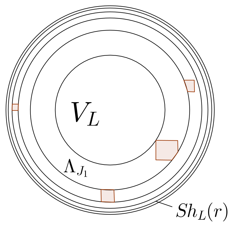
Figure 3: The layers $\Lambda_{j}$, $0\leq j\leq J_{1}$, with $\Lambda_{0}=\operatorname{Sh}_{L}(2r)$. Subsets $D_{\bf k}^{(j)}\subset\Lambda_{j}$ containing bad points are shaded.

Notice that $R\in\mathbb{N}$ can be chosen to depend on the dimension only. Then the events $\{D$ is bad$\}$, $D\in\mathcal{Q}_{j,r}^{(m)}$, are independent. Further, if $L_{1}\leq L\leq L_{1}(\log L_{1})^{2}$, it follows that under $\operatorname{\bf{C1}}(\delta,L_{1})$,

$$\mathbb{P}\left(D\mbox{ is bad}\right)\leq C(r2^{j})^{2d}\exp\left(-\left(\log(r2^{j}/20)\right)^{2}\right)\leq\exp\left(-\left(\log r+j\right)^{5/3}\right)=p_{j,r},$$

for all $r\geq r_{0}$ and $j\in\mathbb{N}$, if $r_{0}$ is big enough. Let $Y_{j,r}$ and $Y_{j,r}^{(m)}$ be the number of bad sets in $\mathcal{Q}_{j,r}$ and $\mathcal{Q}_{j,r}^{(m)}$, respectively. For $r\geq 5$, we have $p_{j,r}\leq(\log r+j)^{-3/2}\leq 1/2$. A standard large deviation estimate for Bernoulli random variables yields

$$\mathbb{P}\left(Y_{j,r}^{(m)}\geq(\log r+j)^{-3/2}N_{j,r}^{(m)}\right)\leq\exp\left(-N_{j,r}^{(m)}\ I\left((\log r+j)^{-3/2}\ \big{|}\ p_{j,r}\right)\right),$$

with $I(x\ |\ p)=x\log(x/p)+(1-x)\log((1-x)/(1-p))$. By enlarging $r_{0}$ if necessary, we get $I\left((\log r+j)^{-3/2}\ |\ p_{j,r}\right)\geq 2R(\log r+j)^{1/7}$ for $r\geq r_{0}$, whence

$$\mathbb{P}\left(Y_{j,r}\geq(\log r+j)^{-3/2}N_{j,r}\right)$$

$$\leq R\max_{m=1,\ldots,R}\mathbb{P}\left(Y_{j,r}^{(m)}\geq(\log r+j)^{-3/2}N_{j,r}^{(m)}\right)\leq R\exp\left(-(\log r+j)^{1/7}N_{j,r}\right)$$

$$\leq R\exp\left(-\frac{1}{C}\ (\log r+j)^{1/7}{\left(\frac{L}{r2^{j}}\right)}^{d-1}\right)\leq\exp\left(-(\log r+j)^{1/7}(\log L)^{29}\right),$$

for $r_{0}\leq r<r_{L}$, $0\leq j\leq J_{1}(L)$ and $L$ large enough. In particular,

$$\sum_{0\leq j\leq J_{1}(L)}\mathbb{P}\left(Y_{j,r}\geq(\log r+j)^{-3/2}N_{j,r}\right)\leq\exp\left(-(\log L)^{28}\right).$$

Therefore, setting

$$\operatorname{BdBad}_{L,r}=\bigcup_{0\leq j\leq J_{1}(L)}\left\{Y_{j,r}\geq(\log r+j)^{-3/2}N_{j,r}\right\},$$

we have proved the following

Lemma 2.2.

There exists a constant $r_{0}>0$ such that if $r\geq r_{0}$ and $L_{1}$ is large enough, then $\operatorname{\bf{C1}}(\delta,L_{1})$ implies that for $L$ with $L_{1}\leq L\leq L_{1}(\log L_{1})^{2}$,

$$\mathbb{P}\left(\operatorname{BdBad}_{L,r}\right)\leq\exp\left(-(\log L)^{28}\right).$$

3 Some important estimates

In this section, we present various results on exit and hitting proababilities for both simple random walk and Brownian motion.

3.1 Hitting probabilities

The first two lemmata concern simple random walk.

Lemma 3.1.

Let $0<\eta<1$.

1. There exists $C=C(\eta)>0$ such that for all $x\in V_{\eta L}$, $y\in\partial V_{L}$,

   $$C^{-1}L^{-d+1}\leq\pi_{L}(x,y)\leq CL^{-d+1}.$$

2. There exists $C=C(\eta)>0$ such that for all $x,x^{\prime}\in V_{\eta L}$, $y\in\partial V_{L}$,

   $$\left|\pi_{L}(x,y)-\pi_{L}(x^{\prime},y)\right|\leq C|x-x^{\prime}|L^{-d}.$$

3. Let $0<l<L$ and $x\in V_{L}$ with $l<|x|<L$. Then

   $$\operatorname{P}_{x}(\tau_{L}<T_{V_{l}})=\frac{l^{-d+2}-|x|^{-d+2}+O(l^{-d+1})}{l^{-d+2}-L^{-d+2}}.$$

Proof: (i) $\pi_{L}(\cdot,y)$ is harmonic inside $V_{L}$. Applying a discrete Harnack inequality, as, for example, provided by Theorem 6.3.9 in the book of Lawler and Limic [24], we see that $C^{-1}\pi_{L}(0,y)\leq\pi_{L}(\cdot,y)\leq C\pi_{L}(0,y)$ on $V_{\eta L}$, for some $C=C(d,\eta)$. Part (i) then follows from Lemma 6.3.7 in the same book.
(ii) By the triangle inequality,

$$\left|\pi_{L}(x,y)-\pi_{L}(x^{\prime},y)\right|\leq C|x-x^{\prime}|\max_{u,v\in V_{\eta L}:|u-v|\leq 1}|\pi_{L}(u,y)-\pi_{L}(v,y)|.$$

For $u\in V_{\eta L}$, the function $\pi_{L}(u+\cdot,y)$ is harmonic inside $V_{(1-\eta)L}$. The claim now follows from [24] Theorem 6.3.8, (6.19), together with (i).
(iii) This is Proposition 1.5.10 of [23]. $\Box$

A good control over hitting probabilities is given by

Lemma 3.2.

Let $a\geq 1$ and $x,y\in\mathbb{Z}^{d}$ with $x\notin V_{a}(y)$. Then

1. $$\operatorname{P}_{x}\left(T_{V_{a}(y)}<\infty\right)=\left(\frac{a}{|x-y|}\right)^{d-2}\left(1+O(a^{-1})\right).$$

2. There exists $C>0$, independent of $a$, such that when $|x-y|>7a$,

   $$\operatorname{P}_{x}\left(T_{V_{a}(y)}<\tau_{L}\right)\leq C\frac{a^{d-2}\max\{a,\operatorname{d}_{L}(y)\}\max\{1,\operatorname{d}_{L}(x)\}}{|x-y|^{d}}.$$

3. There exists $C>0$ such that for all $x\in V_{L}$, $y\in\partial V_{L}$,

   $$C^{-1}\frac{\operatorname{d}_{L}(x)}{|x-y|^{d}}\leq\pi_{L}(x,y)\leq C\frac{\max\{1,\operatorname{d}_{L}(x)\}}{|x-y|^{d}}.$$

This lemma will be proved in the appendix.

We need analogous results for Brownian motion in $\mathbb{R}^{d}$. Denote by $\pi^{\textup{BM}}_{L}(y,dz)$ the exit measure of $d$-dimensional Brownian motion from $C_{L}$, started at $y\in C_{L}$. By a small abuse of notation, we also write $\pi^{\textup{BM}}_{L}(y,z)$ for the (continuous version of the) density with respect to surface measure on $C_{L}$, which is given by the Poisson kernel

$$\pi^{\textup{BM}}_{L}(y,z)=\frac{1}{d\,\alpha(d)\,L}\frac{L^{2}-|y|^{2}}{|y-z|^{d}},$$ (8)

where $\alpha(d)$ is the volume of the unit ball. From this explicit form, we can directly read off the analogous statements of Lemma 3.1 (i), (ii) and Lemma 3.2 (iii), with $V_{L}$ replaced by $C_{L}$. Let us now formulate and prove the analog of parts (i) and (ii) from the last lemma. Denote by $\operatorname{P}^{\textup{BM}}_{x}$ the law of standard $d$-dimensional Brownian motion, started at $x\in\mathbb{R}^{d}$. For the following statement, $T_{C_{a}(y)}$ and $\tau_{C_{L}}$ are defined in the obvious way in terms of Brownian motion.

Lemma 3.3.

Let $a>0$ and $x,y\in\mathbb{R}^{d}$ with $x\notin C_{a}(y)$. Then

1. $$\operatorname{P}^{\textup{BM}}_{x}\left(T_{C_{a}(y)}<\infty\right)=\left(\frac{a}{|x-y|}\right)^{d-2}.$$

2. Assume $C_{2a}(y)\subset C_{L}$. There exists $K>0$ such that

   $$\operatorname{P}^{\textup{BM}}_{x}\left(T_{C_{a}(y)}<\tau_{C_{L}}\right)\leq K\frac{a^{d-2}\operatorname{d}_{L}(y)\operatorname{d}_{L}(x)}{|x-y|^{d}}.$$

Proof of Lemma 3.3: (i) See for example the book of Durrett [12], $(1.12)$.
(ii) Recall that the Green’s function of Brownian motion for $C_{L}$ is given by

$$g^{\textup{BM}}(x,y)=A_{d}\left(\left(\frac{1}{|x-y|}\right)^{d-2}-\left(\frac{L}{\left|x\right|\left|x^{\star}-y\right|}\right)^{d-2}\right),$$

where $A_{d}$ is an explicit constant, and for $x\neq 0$, $x^{\star}=(L^{2}/|x|^{2})x$ is the inversion of $x$ with respect to $C_{L}$. Now, for $a>0$ and $x\notin C_{a}(y)$, we have

$$\int\limits_{C_{a/2}(y)}g^{\textup{BM}}(x,z)\textup{d}z\geq\operatorname{P}^{\textup{BM}}_{x}\left(T_{C_{a}(y)}<\tau_{C_{L}}\right)\inf\limits_{v\in\partial C_{a}(y)}\int\limits_{C_{a/2}(y)}g^{\textup{BM}}(v,z)\textup{d}z.$$

By Proposition $1$ of [10], the infimum on the right-hand side can be bounded from below by $c\,a^{2}$. Using the second upper bound on $g^{\textup{BM}}(x,z)$ from the same proposition, we get

$$\operatorname{P}^{\textup{BM}}_{x}\left(T_{C_{a}(y)}<\tau_{C_{L}}\right)\leq c^{-1}a^{-2}\int\limits_{C_{a/2}(y)}g^{\textup{BM}}(x,z)\textup{d}z\leq K\,\frac{a^{d-2}\operatorname{d}_{L}(y)\operatorname{d}_{L}(x)}{|x-y|^{d}}.$$

$\Box$

Remark 3.1.

Lemma 3.2 (ii) can be proved in the same way if $|x|,|y|\leq cL$ for some $c<1$, for example by using Proposition 8.4.1 of [24], which is based on a coupling argument. Since we need an estimate including the case when $x$ or $y$ are near the boundary, we give a self-contained proof in the appendix.

Probabilities of the above type will often be estimated by the following

Lemma 3.4.

Let $a>0$, $l,m\geq 1$ and $x\in\mathbb{Z}^{d}$. Set $R_{l}=V_{l}\backslash V_{l-1}$, $\alpha=\max\left\{\left||x|-l\right|,a\right\}$. Then for some constant $C=C(m)>0$

$$\sum_{y\in R_{l}}\frac{1}{\left(a+|x-y|\right)^{m}}\leq C\left\{\begin{array}[]{l@{\quad\mbox{\textup{for}\ }}l}l^{d-(m+1)}&1\leq m<d-1\\ \max\{\log(l/\alpha),1\}&m=d-1\\ \alpha^{d-(m+1)}&m\geq d\end{array}\right..$$

Proof: If $\alpha>l$, then the left-hand side is bounded by

$$Cl^{d-1}\alpha^{-m}\leq C\max\left\{\alpha^{d-(m+1)},l^{d-(m+1)}\right\}.$$

If $\alpha\leq l$, we set $A_{k}=\{y\in R_{l}:|x-y|\in[(k-1)\alpha,k\alpha)\}$. Then, for all $k\geq 1$,

$$\max_{y\in A_{k}}\frac{1}{\left(a+|x-y|\right)^{m}}\leq 2^{m}k^{-m}\alpha^{-m}.$$

Since for $k\alpha\leq l/10$ we have $|A_{k}|\leq C\alpha(k\alpha)^{d-2}$, the claim then follows from

$$\sum_{y\in R_{l}}\frac{1}{\left(a+|x-y|\right)^{m}} \leq C\left(\sum_{1\leq k\leq\lfloor l/(10\alpha)\rfloor}\frac{\alpha(k\alpha)^{d-2}}{(k\alpha)^{m}}\right)+Cl^{d-1}l^{-m}$$

$$\leq C\alpha^{d-{(m+1)}}\sum_{1\leq k\leq\lfloor l/(10\alpha)\rfloor}k^{d-(m+2)}+Cl^{d-(m+1)}.$$

$\Box$

3.2 Smoothed exit measures

We will compare exit laws of simple random walk with exit laws of Brownian motion. Given a field of positive real numbers $\psi=\left(m_{x}\right)_{x\in\mathbb{R}^{d}}$, we define the smoothed exit law from $V_{L}$ of simple random walk as

$$\phi_{L,\psi}(x,z)=\pi_{L}\hat{\pi}_{\psi}(x,z)=\sum_{y\in\partial V_{L}}\pi_{L}(x,y)\frac{1}{m_{y}}\int_{\mathbb{R}_{+}}\varphi\left(\frac{t}{m_{y}}\right)\pi_{V_{t}(y)}(y,z)\textup{d}t.$$

Denoting by $\pi^{\textup{BM}}_{C_{t}(x)}(x,dz)$ the exit measure of $d$-dimensional Brownian motion from $C_{t}(x)$, started at $x$, we let analogous to (1),

$$\hat{\pi}^{\textup{BM}}_{\psi}(x,dz)=\frac{1}{m_{x}}\int_{\mathbb{R}_{+}}\varphi\left(\frac{t}{m_{x}}\right)\pi^{\textup{BM}}_{C_{t}(x)}(x,dz)\textup{d}t.$$

Then define the smoothed Brownian exit measure from $C_{L}$ as

$$\phi^{\textup{BM}}_{L,\psi}(x,dz)=\pi^{\textup{BM}}_{L}\hat{\pi}^{\textup{BM}}_{\psi}(x,dz)=\int_{\partial C_{L}}\pi^{\textup{BM}}_{L}(x,dy)\frac{1}{m_{y}}\int_{\mathbb{R}_{+}}\varphi\left(\frac{t}{m_{y}}\right)\pi^{\textup{BM}}_{C_{t}(y)}(y,dz)\textup{d}t.$$

By $\phi^{\textup{BM}}_{L,\psi}(x,z)$ we denote the density of $\phi^{\textup{BM}}_{L,\psi}(x,dz)$ with respect to $d$-dimensional Lebesgue measure.

Lemma 3.5.

Let $\psi\in\mathcal{M}_{L}$. There exists a constant $C>0$ such that

1. $$\sup_{x\in V_{L}}\sup_{z\in\mathbb{Z}^{d}}\left|\left(\phi_{L,\psi}-\phi^{\textup{BM}}_{L,\psi}\right)(x,z)\right|\leq CL^{-(d+1/4)}.$$

2. $$\sup_{z\in\mathbb{R}^{d}}{\left|\left|D^{i}\phi^{\textup{BM}}_{L,\psi}(\cdot,z)\right|\right|}_{C_{L}}\leq CL^{-(d+i)},\quad i=0,1,2,3.$$

3. $$\sup_{x,x^{\prime}\in V_{L}\cup\partial V_{L}}\sup_{z\in\mathbb{Z}^{d}}\left|\phi_{L,\psi}(x,z)-\phi_{L,\psi}(x^{\prime},z)\right|\leq C\left(L^{-(d+1/4)}+|x-x^{\prime}|L^{-(d+1)}\right).$$

For the proof, we refer to the appendix. The next proposition will be applied at the end of the proof of Lemma 5.2. At this point, the invariance condition $\operatorname{\bf{A1}}$ comes into play. We give a general formulation in terms of a signed measure $\nu$. Let us introduce the following notation. For $x=(x_{1},\ldots,x_{d})\in\mathbb{Z}^{d}$, put

$$x^{(i)} = \left(x_{1},\ldots,x_{i-1},-x_{i},x_{i+1},\ldots,x_{d}\right),$$

$$x^{\leftrightarrow(i,j)} = \left(x_{1},\ldots,x_{i-1},x_{j},x_{i+1},\ldots,x_{j-1},x_{i},x_{j+1},\ldots,x_{d}\right),\,\textup{if }i<j.$$

Proposition 3.1.

Let $l>0$. Consider a measure $\nu$ on $V_{l}$ with total mass zero satisfying

1. $\nu(x)=\nu(x^{(i)})$ for all $x$ and all $i=1,\ldots,d$.

2. $\nu(x)=\nu(x^{\leftrightarrow(i,j)})$ for all $x$ and all $i,j=1,\ldots,d$, $i<j$.

Then there exists $C>0$ such that for $y^{\prime}\in V_{L}$ with $V_{l}(y^{\prime})\subset V_{L}$ and all $z\in\mathbb{Z}^{d}$, $\psi\in\mathcal{M}_{L}$,

$$\left|\sum_{y\in V_{l}(y^{\prime})}\nu(y-y^{\prime})\phi_{L,\psi}(y,z)\right|\leq C||\nu||_{1}\left(L^{-(d+1/4)}+\left(\frac{l}{L}\right)^{3}L^{-d}\right).$$

Proof: Since the proof is the same for all $y^{\prime}\in V_{L}$ with $V_{l}(y^{\prime})\subset V_{L}$, we can assume $y^{\prime}=0$. By Lemma 3.5 (i),

$$\left|\sum_{y}\nu(y)\phi_{L,\psi}(y,z)-\sum_{y}\nu(y)\phi^{\textup{BM}}_{L,\psi}(y,z)\right|\leq C||\nu||_{1}L^{-(d+1/4)}.$$

Taylor’s expansion gives

$$\sum_{y}\nu(y)\phi^{\textup{BM}}_{L,\psi}(y,z)$$

$$= \sum_{y}\nu(y)\left[\phi^{\textup{BM}}_{L,\psi}(y,z)-\phi^{\textup{BM}}_{L,\psi}(0,z)\right]$$

$$= \sum_{y}\nu(y)\nabla_{x}\phi^{\textup{BM}}_{L,\psi}(0,z)\cdot y+\ \frac{1}{2}\sum_{y}\nu(y)y\cdot H_{x}\phi^{\textup{BM}}_{L,\psi}(0,z)y+R(\nu,0,z),$$

where $\nabla_{x}\phi^{\textup{BM}}_{L,\psi}$ is the gradient, $H_{x}\phi^{\textup{BM}}_{L,\psi}$ the Hessian of $\phi^{\textup{BM}}_{L,\psi}$ with respect to the first variable, and $R(\nu,0,z)$ is the remainder term, which can be bounded by Lemma 3.5 (ii), namely

$$|R(\nu,0,z)|\leq C||\nu||_{1}\left(\frac{l}{L}\right)^{3}L^{-d}.$$

Since $\nu$ satisfies property (i), the first summand on the right side of (3.2) vanishes. Due to the same reason, the second summand equals

$$\frac{1}{2}\sum_{i=1}^{d}\frac{\partial^{2}}{\partial x_{i}^{2}}\phi^{\textup{BM}}_{L,\psi}(0,z)\sum_{y}\nu(y)(y_{i})^{2}.$$

By property (ii), the sum over $y$ does not depend on $i$, so a multiple of the Laplacian of $\phi^{\textup{BM}}_{L,\psi}$ remains. But for each $v\in\partial C_{L}$, $\pi^{\textup{BM}}_{L}(\cdot,v)$ is harmonic in $C_{L}$, thus also the Laplacian vanishes. This proves the proposition. $\Box$

4 Green’s functions for the ball

One principal task of our approach aims at developing good estimates on Green’s functions for the ball of both coarse grained (goodified) RWRE as well as coarse grained simple random walk. The main result is Lemma 4.1. For the coarse grained simple random walk, the estimates on hitting probabilities of the last section together with Proposition 4.2 yield the right control.

On a certain class of environments, we need to modify the transition kernels in order to ensure that bad points are not visited too often by the coarse grained random walks. This modification will be described in Section 4.4.

4.1 A local central limit theorem

Let $m\geq 1$. Denote by $\hat{\pi}_{m}$ the coarse grained transition probabilities on $\mathbb{Z}^{d}$ belonging to the field $\psi={(m_{x})}_{x\in\mathbb{Z}^{d}}$, where $m_{x}=m$ is chosen constant in $x$. Notice that $\hat{\pi}_{m}$ is centered, and the covariances satisfy

$$\sum_{y\in\mathbb{Z}^{d}}(y_{i}-x_{i})(y_{j}-x_{j})\hat{\pi}_{m}(x,y)=\gamma_{m}\delta_{i}(j),$$

where for large $m$ (recall the coarse graining scheme) $1/d<\gamma_{m}/m^{2}<4/d$.

Proposition 4.1 (Local central limit theorem).

Let $x,y\in\mathbb{Z}^{d}$. For $m\geq 1$ and all integers $n\geq 1$,

$$\hat{\pi}_{m}^{n}(x,y)=\frac{1}{(2\pi\gamma_{m}n)^{d/2}}\exp\left(-\frac{|x-y|^{2}}{2\gamma_{m}n}\right)+O\left(m^{-d}n^{-(d+2)/2}\right).$$

For the corresponding Green’s function $\hat{g}_{m,{\mathbb{Z}^{d}}}(x,y)=\sum_{n=0}^{\infty}\hat{\pi}_{m}^{n}(x,y)$ we obtain

Proposition 4.2.

Let $x,y\in\mathbb{Z}^{d}$. There exists $m_{0}>0$ such that if $m\geq m_{0}$, then

1. For $|x-y|<3m$,

   $$\hat{g}_{m,{\mathbb{Z}^{d}}}(x,y)=\delta_{x}(y)+O(m^{-d}).$$

2. For $|x-y|\geq 3m$, there exists a constant $c(d)>0$ such that

   $$\hat{g}_{m,{\mathbb{Z}^{d}}}(x,y)=\frac{c(d)}{\gamma_{m}|x-y|^{d-2}}+O\left(\frac{1}{|x-y|^{d}}\left(\log\frac{|x-y|}{m}\right)^{d}\right).$$

Here, the constants in the $O$-notation are independent of $m$ and $|x-y|$.

In our applications, $m$ will be a function of $L$. Although these results look rather standard, we cannot directly refer to the literature because we have to keep track of the $m$-dependency. We give a proof of both statements in the appendix.

We will use the last proposition to estimate the Green’s function for the ball $V_{L}$, $\hat{g}_{m}(x,y)=\sum_{n=0}^{\infty}\left(1_{V_{L}}\hat{\pi}_{m}\right)^{n}(x,y)$. Clearly, $\hat{g}_{m}$ is bounded from above by $\hat{g}_{m,{\mathbb{Z}^{d}}}$, and more precisely, the strong Markov property shows

$$\hat{g}_{m}(x,y)=\operatorname{E}_{x,\hat{\pi}_{m}}\left[\sum_{k=0}^{\tau_{L}-1}1_{\{X_{k}=y\}}\right]=\hat{g}_{m,\mathbb{Z}^{d}}(x,y)-\operatorname{E}_{x,\hat{\pi}_{m}}\left[\hat{g}_{m,\mathbb{Z}^{d}}\left(X_{\tau_{L}},y\right)\right].$$ (10)

4.2 Estimates on coarse grained Green’s functions

As we will show, the perturbation expansion enables us to control the goodified Green’s function $\hat{G}^{g}_{L,r}$ essentially in terms of $\hat{g}_{L,r}$. The boundary region $\operatorname{Sh}_{L}(r)$ turns out to be problematic, since even for good $x$, we cannot estimate the variational distance between the transition kernels by $\delta$. We therefore work in this (and only in this) section with slightly modified transition kernels $\tilde{\Pi}_{L,r}$, $\tilde{\pi}_{L,r}$, $\tilde{\Pi}^{g}_{L,r}$ in the enlarged ball $V_{L+r}$, taking the exit measure in $\operatorname{Sh}_{L}(r)$ from uncut balls $V_{t}(x)\subset V_{L+r}$, $t\in[h_{L,r}(x),2h_{L,r}(x)]$. More precisely, setting $h_{L,r}(x)=(1/20)r$ for $x\notin C_{L}$, we let $\tilde{\pi}_{L,r}$ be the coarse grained simple random walk kernel under $\tilde{\psi}=(h_{L,r}(x))_{x\in V_{L+r}}$, that is

$$\tilde{\pi}_{L,r}(x,\cdot)=\frac{1}{h_{L,r}(x)}\int_{\mathbb{R}_{+}}\varphi\left(\frac{t}{h_{L,r}(x)}\right)\pi_{V_{t}(x)\cap V_{L+r}}(x,\cdot)\textup{d}t.$$

For the corresponding RWRE kernel, we forget about the environment on $V_{L+r}\backslash V_{L}$ and set

$$\tilde{\Pi}_{L,r}(x,\cdot)=\left\{\begin{array}[]{l@{\quad\mbox{for\ }}l}\frac{1}{h_{L,r}(x)}\int_{\mathbb{R}_{+}}\varphi\left(\frac{t}{h_{L,r}(x)}\right)\Pi_{V_{t}(x)}(x,\cdot)\textup{d}t&x\in V_{L}\\ \tilde{\pi}_{L,r}(x,\cdot)&x\in V_{L+r}\backslash V_{L}\end{array}\right..$$

For all good $x\in V_{L}$ we now have $||(\tilde{\Pi}_{L,r}-\tilde{\pi}_{L,r})(x,\cdot)||_{1}\leq\delta$, while for $x\in V_{L+r}\backslash V_{L}$, the difference vanishes anyway. The goodified version of $\tilde{\Pi}_{L,r}$ is then obtained in an analogous way to (7),

$$\tilde{\Pi}^{g}_{L,r}(x,\cdot)=\left\{\begin{array}[]{l@{\quad\mbox{for\ }}l}\tilde{\Pi}_{L,r}(x,\cdot)&x\notin\mathcal{B}^{\star}_{L,r}\\ \tilde{\pi}_{L,r}(x,\cdot)&x\in\mathcal{B}^{\star}_{L,r}\end{array}\right..$$

We write $\tilde{G}_{L,r},\tilde{g}_{L,r}$ and $\tilde{G}^{g}_{L,r}$ for the corresponding Green’s functions on $V_{L+r}$. Note that

$$\hat{G}_{L,r}\leq\tilde{G}_{L,r},\quad\hat{g}_{L,r}\leq\tilde{g}_{L,r},\quad\hat{G}^{g}_{L,r}\leq\tilde{G}^{g}_{L,r}\quad\mbox{pointwise on }V_{L+r}\times\left(V_{L+r}\backslash\partial V_{L}\right).$$ (11)

Since we do not have exact expressions for $\tilde{g}_{L,r}$ or $\tilde{G}_{L,r}$, we will construct a (deterministic) kernel $\Gamma_{L,r}$ that bounds the Green’s functions from above. For $x\in V_{L+r}$, set

$$\operatorname{\tilde{d}}(x)=\max\left(\frac{\operatorname{d}_{L+r}(x)}{2},3r\right),\quad a(x)=\min\left(\operatorname{\tilde{d}}(x),s_{L}\right).$$

Further, let

$$\Gamma^{(1)}_{L,r}(x,y)=\frac{\tilde{d}(x)\tilde{d}(y)}{a(y)^{2}(a(y)+|x-y|)^{d}},\quad\Gamma^{(2)}_{L,r}(x,y)=\frac{1}{a(y)^{2}(a(y)+|x-y|)^{d-2}}.$$

The kernel $\Gamma_{L,r}$ is defined as the pointwise minimum

$$\Gamma_{L,r}=\min\left\{\Gamma^{(1)}_{L,r},\Gamma^{(2)}_{L,r}\right\}.$$ (12)

We cannot derive pointwise estimates on the Green’s functions in terms of $\Gamma_{L,r}$, but we can use this kernel to obtain upper bounds on neighborhoods $U(x)=V_{a(x)}(x)\cap V_{L+r}$. Call a function $F:V_{L+r}\times V_{L+r}\rightarrow\mathbb{R}_{+}$ a positive kernel. Given two positive kernels $F$ and $G$, we write $F\preceq G$ if for all $x,y\in V_{L+r}$,

$$F(x,U(y))\leq G(x,U(y)),$$

where $F(x,U)$ stands for $\sum_{y\in U\cap\mathbb{Z}^{d}}F(x,y)$. Further, we write $F\asymp 1$, if there is a constant $C>0$ such that for all $x,y\in V_{L+r}$,

$$\frac{1}{C}F(x,y)\leq F(\cdot,\cdot)\leq CF(x,y)\quad\mbox{on }U(x)\times U(y).$$

We adopt this notation to positive functions of one argument: For $f:V_{L+r}\rightarrow\mathbb{R}_{+}$, $f\asymp 1$ means that for some $C>0$, $C^{-1}f(x)\leq f(\cdot)\leq Cf(x)$ on any $U(x)\subset V_{L+r}$. Finally, given $0<\eta<1$, we say that a positive kernel $A$ on $V_{L+r}$ is $\eta$-smoothing, if for all $x\in V_{L+r}$, $A(x,U(x))\leq\eta$, and $A(x,y)=0$ whenever $y\notin U(x)$.

Now we are in the position to formulate our main statement of this section. Recall our convention concerning constants: They only depend on the dimension unless stated otherwise.

Lemma 4.1.

1. There exists a constant $C_{1}>0$ such that

   $$\hat{g}_{L,r}\preceq C_{1}\Gamma_{L,r}\quad\mbox{and}\quad\tilde{g}_{L,r}\preceq C_{1}\Gamma_{L,r}.$$

2. There exists a constant $C>0$ such that for small $\delta>0$,

   $$\hat{G}^{g}_{L,r}\preceq C\Gamma_{L,r}\quad\mbox{and}\quad\tilde{G}^{g}_{L,r}\preceq C\Gamma_{L,r}.$$

Remark 4.1.

Thanks to (11), it suffices to prove the bounds for $\tilde{g}_{L,r}$ and $\tilde{G}^{g}_{L,r}$. For later use, we keep track of the constant in part (i) of the lemma.

We first prove part (i), which is a straightforward consequence of the estimates on hitting probabilities in Section 3 and the next lemma.

Lemma 4.2.

There exists $C>0$ such that for all $x\in V_{L+r}$ and $y\in V_{L}$ with $\operatorname{d}_{L}(y)\geq 4s_{L}$,

$$\tilde{g}_{L,r}(x,y)\leq C\left\{\begin{array}[]{l@{,\quad}l}\frac{1}{s_{L}^{2}\max\{|x-y|,s_{L}\}^{d-2}}&y\neq x\\ 1&y=x\end{array}\right..$$

Proof: If $x=y$, then the claim follows from transience of simple random walk. Now assume $x\neq y$, and always $\operatorname{d}_{L}(y)\geq 4s_{L}$. Consider first the case $|x-y|\leq s_{L}$. Let $\hat{g}_{m}$ be defined as in the beginning of Section 4.1. Recall our coarse graining scheme. With $m=s_{L}/20$ we have

$$\tilde{g}(x,y)\leq\hat{g}_{m}(x,y)+\sup_{v\in\operatorname{Sh}_{L}(2s_{L})}\operatorname{P}_{v}\left(T_{V_{s_{L}}(y)}<\tau_{V_{L+r}}\right)\sup_{w:w\neq y,\atop|w-y|\leq s_{L}}\tilde{g}(w,y).$$

Since

$$\sup_{v\in\operatorname{Sh}_{L}(2s_{L})}\operatorname{P}_{v}\left(T_{V_{s_{L}}(y)}<\tau_{V_{L+r}}\right)<1$$

uniformly in $L$, it follows from Proposition 4.2 that

$$\tilde{g}(x,y)\leq C\sup_{w:w\neq y,\atop|w-y|\leq s_{L}}\hat{g}_{m}(w,y)\leq C\sup_{w:w\neq y,\atop|w-y|\leq s_{L}}\hat{g}_{m,\mathbb{Z}^{d}}(w,y)\leq\frac{C}{s_{L}^{d}}.$$

If $|x-y|>s_{L}$ we use Lemma 3.2 (i) and the first case to get

$$\tilde{g}(x,y)\leq\operatorname{P}_{x}\left(T_{V_{s_{L}}(y)}<\infty\right)\sup_{w:w\neq y,\atop|w-y|\leq s_{L}}\tilde{g}(w,y)\leq\frac{C}{s_{L}^{2}|x-y|^{d-2}}.$$

$\Box$

Proof of Lemma 4.1 (i): It suffices to prove the bound for $\tilde{g}$. First we show that there exists a constant $C>0$ such that for all $y\in V_{L+r}$,

$$\sup_{x\in V_{L+r}}\tilde{g}\left(x,U(y)\right)\leq C.$$ (13)

At first let $\operatorname{d}_{L+r}(y)\leq 6r$. Then $U(y)\subset\operatorname{Sh}_{L+r}(10r)$. We claim that

$$\sup_{x\in V_{L+r}}\tilde{g}\left(x,\operatorname{Sh}_{L+r}(10r)\right)\leq C.$$ (14)

for some $C>0$. Indeed, if $z\in\operatorname{Sh}_{L+r}(10r)$, then $\tilde{\pi}(z,\cdot)$ is an (averaging) exit distribution from balls $V_{l}(z)\cap V_{L+r}$, where $l\geq r/20$. Using Lemma 3.1 (i), we find a constant $k_{1}=k_{1}(d)$ such that starting at any $z\in\operatorname{Sh}_{L+r}(10r)$, $V_{L+r}$ is left after $k_{1}$ steps with probability $>0$, uniformly in $z$. This together with the strong Markov property implies (14). Next assume $6r<\operatorname{d}_{L+r}(y)\leq 6s_{L}$. Then $U(y)\subset S(y)=\operatorname{Sh}_{L+r}\left(\frac{1}{2}\operatorname{d}_{L+r}(y),2\operatorname{d}_{L+r}(y)\right)$. We claim that

$$\sup_{x\in V_{L+r}}\tilde{g}\left(x,S(y)\right)\leq C.$$ (15)

For $z\in S(y)$, $\tilde{\pi}(z,\cdot)$ is an averaging exit distribution from balls $V_{l}(z)$, where $l\geq\operatorname{d}_{L+r}(y)/240$. By Lemma 3.1 (i), we find some small $0<c<1$ and a constant $k_{2}(c,d)$ such that after $k_{2}$ steps, the walk has probability $>0$ to be in $\operatorname{Sh}_{L+r}\left(\frac{1-c}{2}\operatorname{d}_{L+r}(y)\right)$, uniformly in $z$ and $y$. But starting in $\operatorname{Sh}_{L+r}\left(\frac{1-c}{2}\operatorname{d}_{L+r}(y)\right)$, Lemma 3.1 (iii) shows that with probability $>0$, the ball $V_{L+r}$ is left before $S(y)$ is visited again. Therefore (15) and hence (13) hold in this case. At last, let $\operatorname{d}_{L+r}(y)>6s_{L}$. Then $\operatorname{d}_{L}(w)\geq 4s_{L}$ for $w\in U(y)$. Estimating

$$\tilde{g}(x,w)\leq 1+\sup_{v:v\neq w}\tilde{g}(v,w),$$

we get with part (i) that

$$\sup_{w\in U(y)}\tilde{g}(x,w)\leq 1+\frac{C}{s_{L}^{d}}.$$

Summing over $w\in U(y)$, (13) follows. Finally, note that for any $x\in V_{L+r}$,

$$\tilde{g}(x,U(y))\leq\operatorname{P}_{x}\left(T_{U(y)}\leq\tau_{V_{L+r}}\right)\sup_{w\in U(y)}\tilde{g}(w,U(y)).$$

Now $\tilde{g}\preceq C\Gamma$ follows from (13) and the hitting estimates of Lemma 3.2. $\Box$

Let us now explain our strategy for proving part (ii). By version (5) of the perturbation expansion, we can express $\tilde{G}^{g}_{L,r}$ in a series involving $\tilde{g}_{L,r}$ and differences of exit measures. The Green’s function $\tilde{g}_{L,r}$ is already controlled by means of $\Gamma_{L,r}$. Looking at (5), we thus have to understand what happens if $\Gamma_{L,r}$ is concatenated with certain smoothing kernels. This will be the content of Proposition 4.3.

We start with collecting some important properties of $\Gamma_{L,r}$, which will be used throughout this text. Define for $j\in\mathbb{N}$

$$\mathcal{L}_{j}=\{y\in V_{L}:j\leq\operatorname{d}_{L}(y)<j+1\},\quad\mathcal{E}_{j}=\{y\in V_{L+r}:\operatorname{\tilde{d}}(y)\leq 3jr\}.$$

Lemma 4.3 (Properties of $\Gamma_{L,r}$).

1. Both $\operatorname{\tilde{d}}$ and $a$ are Lipschitz with constant $1/2$. Moreover, for $x,y\in V_{L+r}$,

   $$a(y)+|x-y|\leq a(x)+\frac{3}{2}|x-y|.$$

2. $$\Gamma_{L,r}\asymp 1.$$

3. For $0\leq j\leq 2s_{L}$, $x\in V_{L+r}$,

   $$\sum_{y\in\mathcal{L}_{j}}\left(\max\left\{1,\frac{\operatorname{\tilde{d}}(x)}{a(y)}\right\}\frac{1}{(a(y)+|x-y|)^{d}}\right)\leq C\frac{1}{j\vee r}.$$

4. For $1\leq j\leq\frac{1}{3r}s_{L}$,

   $$\sup_{x\in V_{L+r}}\Gamma_{L,r}(x,\mathcal{E}_{j})\leq C\log(j+1),$$

   and for $0\leq\alpha<3$,

   $$\sup_{x\in V_{L+r}}\Gamma_{L,r}\left(x,\operatorname{Sh}_{L}\left(s_{L},L/(\log L)^{\alpha}\right)\right)\leq C(\log\log L)(\log L)^{6-2\alpha}.$$

5. For $x\in V_{L+r}$, in the case of constant $r$,

   $$\Gamma_{L,r}(x,V_{L})\leq C\max\left\{\frac{\operatorname{\tilde{d}}(x)}{L}(\log L)^{6},\,\left(\frac{\operatorname{\tilde{d}}(x)}{r}\wedge\log L\right)\right\}.$$

   In the case $r=r_{L}$,

   $$\Gamma_{L,r_{L}}(x,V_{L})\leq C\max\left\{\frac{\operatorname{\tilde{d}}(x)}{L}(\log L)^{6},\,\left(\frac{\operatorname{\tilde{d}}(x)}{r_{L}}\wedge\log\log L\right)\right\}.$$

Proof: (i) The second statement is a direct consequence of the Lipschitz property, which in turn follows immediately from the definitions of $\operatorname{\tilde{d}}$ and $a$.
(ii) As for $y^{\prime}\in U(y)$, $\frac{1}{2}a(y)\leq a(y^{\prime})\leq\frac{3}{2}a(y)$ and similarly with $a$ replaced by $\operatorname{\tilde{d}}$, it suffices to show that for $x^{\prime}\in U(x)$, $y^{\prime}\in U(y)$,

$$\frac{1}{C}\left(a(y)+|x-y|\right)\leq a(y^{\prime})+|x^{\prime}-y^{\prime}|\leq C\left(a(y)+|x-y|\right).$$ (16)

First consider the case $|x-y|\geq 4\max\{a(x),a(y)\}$. Then

$$a(y)+|x-y|\leq 2a(y^{\prime})+2\left(|x-y|-a(x)-a(y)\right)\leq 2\left(a(y^{\prime})+|x^{\prime}-y^{\prime}|\right).$$

If $|x-y|\leq 4a(y)$ then

$$a(y)+|x-y|\leq 5a(y)\leq 5a(y)+|x^{\prime}-y^{\prime}|\leq 10\left(a(y^{\prime})+|x^{\prime}-y^{\prime}|\right),$$

while for $|x-y|\leq 4a(x)$, using part (i) in the first inequality,

$$a(y)+|x-y|\leq a(x)+\frac{3}{2}|x-y|\leq 7a(x)\leq 14\left(a(y^{\prime})+|x^{\prime}-y^{\prime}|\right).$$

This proves the first inequality in (16). The second one follows from

$$a(y^{\prime})+|x^{\prime}-y^{\prime}|\leq\frac{5}{2}a(y)+a(x)+|x-y|\leq\frac{7}{2}\left(a(y)+|x-y|\right).$$

(iii) If $j\leq 2s_{L}$ and $y\in\mathcal{L}_{j}$, then $a(y)$ is of order $j\vee r$. By Lemma 3.4 we have

$$\sum_{y\in\mathcal{L}_{j}}\frac{1}{(j\vee r+|x-y|)^{d}}\leq C\min\left\{\frac{1}{j\vee r},\frac{1}{\left|\operatorname{d}_{L+r}(x)-(j+r)\right|}\right\}.$$

It remains to show that

$$\max\left\{1,\frac{\operatorname{\tilde{d}}(x)}{j\vee r}\right\}\min\left\{\frac{1}{j\vee r},\frac{1}{\left|\operatorname{d}_{L+r}(x)-(j+r)\right|}\right\}\leq C\frac{1}{j\vee r}.$$ (17)

If $\operatorname{\tilde{d}}(x)\leq(j\vee 3r)$, this is clear. If $\operatorname{\tilde{d}}(x)>(j\vee 3r)$,  (17) follows from $|\operatorname{d}_{L+r}(x)-(j+r)|\geq\operatorname{\tilde{d}}(x)/2$.
(iv) If $\operatorname{\tilde{d}}(y)\leq 3jr$, then $\operatorname{d}_{L}(y)\leq 6jr$. Estimating $\Gamma$ by $\Gamma^{(1)}$, we get

$$\Gamma(x,\mathcal{E}_{j})\leq C\sum_{i=0}^{6jr}\sum_{y\in\mathcal{L}_{i}}\frac{\operatorname{\tilde{d}}(x)}{a(y)}\frac{1}{(a(y)+|x-y|)^{d}}.$$

Now the first assertion of (iv) follows from (iii). The second is proved similarly, so we omit the details.
(v) Set $B=\{y\in V_{L}:\operatorname{\tilde{d}}(y)\leq s_{L}\vee 2\operatorname{\tilde{d}}(x)\}$. For $y\in V_{L}\backslash B$, it holds that $a(y)=s_{L}$ and $|x-y|\geq\operatorname{\tilde{d}}(y)$. Therefore,

$$\Gamma\left(x,V_{L}\backslash B\right)\leq\Gamma^{(1)}\left(x,V_{L}\backslash B\right)\leq\frac{\operatorname{\tilde{d}}(x)}{s_{L}^{2}}\sum_{y\in V_{2L}}\frac{1}{(s_{L}+|y|)^{d-1}}\leq C\frac{\operatorname{\tilde{d}}(x)}{L}(\log L)^{6}.$$

Furthermore,

$$\Gamma\left(x,B\right)\leq\sum_{i=0}^{2s_{L}}\sum_{y\in\mathcal{L}_{i}}\frac{\operatorname{\tilde{d}}(x)}{a(y)}\frac{1}{(a(y)+|x-y|)^{d}}+\frac{1}{s_{L}^{2}}\sum_{y\in V_{L}:\atop s_{L}\leq\operatorname{\tilde{d}}(y)\leq 2\operatorname{\tilde{d}}(x)}\frac{1}{(s_{L}+|x-y|)^{d-2}}.$$

Lemma 3.4 bounds the second term by $C(\operatorname{\tilde{d}}(x)/L)(\log L)^{6}$. For the first term, we use twice part (iii) and once Lemma 3.4 to get

$$\sum_{i=0}^{2s_{L}}\sum_{y\in\mathcal{L}_{i}}\frac{\operatorname{\tilde{d}}(x)}{a(y)}\frac{1}{(a(y)+|x-y|)^{d}}\leq C\sum_{i=0}^{5r}\frac{1}{i\vee r}+C\min\left\{\operatorname{\tilde{d}}(x)\sum_{i=5r}^{2s_{L}}\frac{1}{i^{2}},\sum_{i=5r}^{2s_{L}}\frac{1}{i}\right\}.$$

This proves (v). $\Box$

Proposition 4.3 (Concatenating).

Let $F,G$ be positive kernels with $F\preceq G$.

1. If $A$ is $\eta$-smoothing and $G\asymp 1$, then for some constant $C=C(d,G)>0$,

   $$FA\preceq C\eta G.$$

2. If $\Phi$ is a positive function on $V_{L+r}$ with $\Phi\asymp 1$, then for some $C=C(d,\Phi)>0$,

   $$F\Phi\leq CG\Phi.$$

Proof: (i) As $a$ is Lipschitz with constant $1/2$, we can choose $K=K(d)$ points $y_{k}$ out of the set $M=\{y^{\prime}\in V_{L+r}:U(y^{\prime})\cap U(y)\neq\emptyset\}$ such that $M$ is covered by the union of the $U(y_{k}),k=1,\ldots,K.$ Since $A(y^{\prime},U(y))\neq 0$ implies $y^{\prime}\in M$, we then have

$$FA(x,U(y)) = \sum_{y^{\prime}\in M}F(x,y^{\prime})\sum_{y^{\prime\prime}\in U(y)}A(y^{\prime},y^{\prime\prime})\leq\eta\sum_{k=1}^{K}F(x,U(y_{k}))$$

$$\leq \eta\sum_{k=1}^{K}G(x,U(y_{k})).$$

Using $G\asymp 1$, we get $G(x,U(y_{k}))\leq C|U(y_{k})|G(x,y)$. Clearly $|U(y_{k})|\leq C|U(y)|$, so that

$$FA(x,U(y))\leq CK\eta|U(y)|G(x,y).$$

A second application of $G\asymp 1$ yields the claim.
(ii) We can find a constant $K=K(d)$ and a covering of $V_{L+r}$ by neighborhoods $U(y_{k})$, $y_{k}\in V_{L+r}$, such that every $y\in V_{L+r}$ is contained in at most $K$ many of the sets $U(y_{k})$. Using $\Phi\asymp 1$, it follows that for $x\in V_{L+r}$,

$$F\Phi(x)=\sum_{y\in V_{L+r}}F(x,y)\Phi(y) \leq C\sum_{k=1}^{\infty}F(x,U(y_{k}))\Phi(y_{k})\leq C\sum_{k=1}^{\infty}G(x,U(y_{k}))\Phi(y_{k})$$

$$\leq C\sum_{k=1}^{\infty}\sum_{y\in U(y_{k})}G(x,y)\Phi(y)\leq CK\sum_{y\in V_{L+r}}G(x,y)\Phi(y).$$

$\Box$

In terms of our specific kernel $\Gamma_{L,r}$, we obtain

Proposition 4.4.

Let $A$ be $\eta$-smoothing, and let $F$ be a positive kernel satisfying $F\preceq\Gamma_{L,r}$.

1. There exists a constant $C_{2}>0$ not depending on $F$ and $A$ such that

   $$FA\preceq C_{2}\eta\Gamma_{L,r}.$$

2. If additionally $A(x,y)=0$ for $x\notin V_{L}$ and $A(x,U(x))\leq\left(\log(a(x)/20)\right)^{-9}$ for $x\in V_{L}\backslash\mathcal{E}_{1}$, then there exists a constant $C_{3}>0$ not depending on $F$ and $A$ such that for all $x,z\in V_{L+r}$,

   $$FA\Gamma_{L,r}(x,z)\leq C_{3}\eta^{1/2}\Gamma_{L,r}(x,z).$$

Proof: (i) This is Proposition 4.3 (i) with $G=\Gamma$.
(ii) We set $B=V_{L}\backslash\mathcal{E}_{1}$ and split into

$$FA\Gamma=F1_{\mathcal{E}_{1}}A\Gamma+F1_{B}A\Gamma.$$ (18)

Let $x,z\in V_{L+r}$ be fixed, and consider first $F1_{\mathcal{E}_{1}}A\Gamma(x,z)$. Using $\Gamma\asymp 1$, $A\Gamma(y,z)\leq C\eta\Gamma(y,z)$. As $\Gamma(\cdot,z)\asymp 1$ and $F1_{\mathcal{E}_{1}}\preceq\Gamma 1_{\mathcal{E}_{2}}$, we get by Proposition 4.3 ii)

$$F1_{\mathcal{E}_{1}}A\Gamma(x,z)\leq C\eta\Gamma 1_{\mathcal{E}_{2}}\Gamma(x,z).$$

Setting $\mathcal{E}_{2}^{1}=\{y\in\mathcal{E}_{2}:|y-z|\geq|x-z|/2\}$, $\mathcal{E}_{2}^{2}=\mathcal{E}_{2}\backslash\mathcal{E}_{2}^{1}$, we split further into

$$\Gamma 1_{\mathcal{E}_{2}}\Gamma=\Gamma 1_{\mathcal{E}_{2}^{1}}\Gamma+\Gamma 1_{\mathcal{E}_{2}^{2}}\Gamma.$$

If $y\in\mathcal{E}_{2}^{1}$, then $\Gamma(y,z)\leq C\Gamma(x,z)$. By Lemma 4.3 (iv), $\Gamma(x,\mathcal{E}_{2})\leq C$. Together we obtain

$$\Gamma 1_{\mathcal{E}_{2}^{1}}\Gamma(x,z)\leq C\Gamma(x,z).$$

If $y\in\mathcal{E}_{2}^{2}$, then $\Gamma(x,y)\leq C\frac{a(z)^{2}}{r^{2}}\Gamma(x,z)$ and $\Gamma^{(1)}(y,z)\leq C\frac{r^{2}}{a(z)^{2}}\Gamma^{(1)}(z,y)$, whence

$$\Gamma 1_{\mathcal{E}_{2}\backslash\mathcal{E}_{2}^{2}}\Gamma(x,z)\leq C\Gamma(x,z)\Gamma^{(1)}(z,\mathcal{E}_{2})\leq C\Gamma(x,z).$$

We therefore have shown that

$$F1_{\mathcal{E}_{1}}A\Gamma(x,z)\leq C\eta\Gamma(x,z).$$

To handle the second summand of (18), set $\sigma(y)=\min\left\{\eta,\left(\log a(y)\right)^{-9}\right\}$, $y\in V_{L+r}$. Clearly, $1_{B}A\Gamma(y,z)\leq C\sigma(y)\Gamma(y,z)$ and $F1_{B}\preceq\Gamma 1_{V_{L}}$. Furthermore, $\sigma(\cdot)\Gamma(\cdot,z)\asymp 1$, so that by Proposition 4.3 ii)

$$F1_{B}A\Gamma(x,z)\leq C\Gamma 1_{V_{L}}\sigma\Gamma(x,z).$$

Consider $D^{1}=\{y\in V_{L}:|y-z|\geq|x-z|/2\}$, $D^{2}=V_{L}\backslash D^{1}$ and split into

$$\Gamma 1_{V_{L}}\sigma\Gamma=\Gamma 1_{D^{1}}\sigma\Gamma+\Gamma 1_{D^{2}}\sigma\Gamma.$$

If $y\in D^{1}$, then $\Gamma(y,z)\leq C\max\left\{1,\frac{\operatorname{\tilde{d}}(y)}{\operatorname{\tilde{d}}(x)}\right\}\Gamma(x,z)$, implying $\Gamma 1_{D^{1}}\sigma\Gamma(x,z)\leq C\eta^{1/2}\Gamma(x,z)$ if we prove

$$\sum_{y\in V_{L}}\max\left\{1,\frac{\operatorname{\tilde{d}}(y)}{\operatorname{\tilde{d}}(x)}\right\}\Gamma(x,y)\sigma(y)\leq C\eta^{1/2}.$$ (19)

To this end, we treat the summation over $S^{1}=\{y\in V_{L}:\operatorname{d}_{L}(y)\leq 2s_{L}\}$ and $S^{2}=V_{L}\backslash S_{1}$ separately. If $y\in S^{2}$, then $a(y)=s_{L}$. Estimating $\Gamma$ by $\Gamma^{(1)}$ and $\operatorname{\tilde{d}}(y)$, $\operatorname{\tilde{d}}(x)$ simply by $L$, we get

$$\sum_{y\in S^{2}}\max\left\{1,\frac{\operatorname{\tilde{d}}(y)}{\operatorname{\tilde{d}}(x)}\right\}\Gamma(x,y)\sigma(y)\leq\frac{C}{(\log L)^{3}}\sum_{y\in V_{2L}}\frac{1}{\left(s_{L}+|y|\right)^{d}}\leq\frac{C\log\log L}{(\log L)^{3}}.$$ (20)

If $y\in S^{1}$, we estimate $\Gamma$ again by $\Gamma^{(1)}$ and split the summation into the layers $\mathcal{L}_{j}$, $j=0,\ldots,2s_{L}$. On $\mathcal{L}_{j}$, $\sigma(y)\leq C\min\left\{\eta,(\log(j+1))^{-9}\right\}$. Thus, by Lemma 4.3 (iii),

$$\sum_{y\in S^{1}}\max\left\{1,\frac{\operatorname{\tilde{d}}(y)}{\operatorname{\tilde{d}}(x)}\right\}\Gamma(x,y)\sigma(y)$$

$$\leq C\sum_{j=0}^{2s_{L}}\sum_{y\in\mathcal{L}_{j}}\max\left\{1,\frac{\operatorname{\tilde{d}}(x)}{a(y)}\right\}\frac{\min\left\{\eta,(\log(j+1))^{-9}\right\}}{(a(y)+|x-y|)^{d}}$$

$$\leq C\sum_{j=0}^{2s_{L}}\frac{\min\left\{\eta,(\log(j+1))^{-9}\right\}}{j\vee r}\leq C\eta^{1/2}.$$

Together with (20), we have proved (19). It remains to bound the term $\Gamma 1_{D^{2}}\sigma\Gamma(x,z)$. But if $y\in D^{2}$, then

$$a(y)+|x-y|\geq a(y)+\frac{1}{2}|x-z|\geq a(z)-\frac{1}{2}|y-z|+\frac{1}{2}|x-z|\geq\frac{1}{4}\left(a(z)+|x-z|\right),$$

whence $\Gamma(x,y)\leq C\frac{a(z)^{2}}{a(y)^{2}}\max\left\{1,\frac{\operatorname{\tilde{d}}(y)}{\operatorname{\tilde{d}}(z)}\right\}\Gamma(x,z)$. Using Lemma 4.3 (i), we have

$$\frac{a(z)^{2}}{a(y)^{2}}\Gamma(y,z)\leq C\Gamma(z,y),$$

so that $\Gamma 1_{D^{2}}\sigma\Gamma(x,z)\leq C\eta^{1/2}\Gamma(x,z)$ follows again from (19). $\Box$

Now we have collected all ingredients to finally prove part (ii) of our main Lemma 4.1. Proof of Lemma 4.1 (ii): As already remarked, we only have to prove the statement involving $\tilde{G}^{g}$. The perturbation expansion (5) yields

$$\tilde{G}^{g}=\tilde{g}\sum_{m=0}^{\infty}(R\tilde{g})^{m}\sum_{k=0}^{\infty}\Delta^{k},$$

where $\Delta=1_{V_{L+r}}(\tilde{\Pi}^{g}-\tilde{\pi})$, $R=\sum_{k=1}^{\infty}\Delta^{k}\tilde{\pi}$. With the constants $C_{1}$ of Lemma 4.1 (i) and $C_{2},C_{3}$ of Proposition 4.4 we choose

$$\delta\leq\frac{1}{16}\left(\frac{1}{C_{2}\vee C_{1}^{2}C_{3}^{2}}\right).$$

From Lemma 4.1 (i) and Proposition 4.4 (i) with $A=|\Delta|$, $\eta=\delta$ we then deduce that $\tilde{g}|\Delta|\preceq(C_{1}/2)\Gamma$, and, by iterating,

$$\sum_{k=1}^{\infty}\tilde{g}|\Delta|^{k-1}\preceq 2C_{1}\Gamma.$$

Furthermore, by part (ii) of Proposition 4.4 with $A=|\Delta\tilde{\pi}|$ and Lemma 4.1 (i),

$$\sum_{k=1}^{\infty}\tilde{g}|\Delta|^{k-1}\left|\Delta\tilde{\pi}\right|\tilde{g}\preceq(C_{1}/2)\Gamma.$$

Repeating this procedure shows that for $m\in\mathbb{N}$,

$$\tilde{g}(|R|\tilde{g})^{m}\preceq C_{1}2^{-m}\Gamma.$$

Finally, by a further application of Proposition 4.4 (i),

$$\tilde{g}\sum_{m=0}^{\infty}(|R|\tilde{g})^{m}\sum_{k=0}^{\infty}|\Delta|^{k}\preceq 4C_{1}\Gamma.$$

This proves the lemma. $\Box$

4.3 Difference estimates

The results from the preceding section enable us to prove some difference estimates on the coarse grained Green’s functions, which will be used in the part on mean sojourn times. The reader who is only interested in the exit measures may skip this section.

Lemma 4.4.

There exists a constant $C>0$ such that

1. $$\sup_{x,x^{\prime}\in V_{L}:|x-x^{\prime}|\leq s_{L}}\sum_{y\in V_{L}}\left|\hat{g}_{L,r}(x,y)-\hat{g}_{L,r}(x^{\prime},y)\right|\leq C(\log\log L)(\log L)^{3}.$$

2. For $\delta>0$ small,

   $$\sup_{x,x^{\prime}\in V_{L}:|x-x^{\prime}|\leq s_{L}}\sum_{y\in V_{L}}\left|\hat{G}^{g}_{L,r_{L}}(x,y)-\hat{G}^{g}_{L,r_{L}}(x^{\prime},y)\right|\leq C(\log\log L)(\log L)^{3}.$$

Proof: (i) Set $m=s_{L}/20$. Recall the definitions of $\hat{\pi}_{m}$ and $\hat{g}_{m}$ from Section 4.1. We write

$$\sum_{y\in V_{L}}\left|\hat{g}(x,y)-\hat{g}(x^{\prime},y)\right|$$

$$\leq \sum_{y\in V_{L}}\left|\left(\hat{g}-\hat{g}_{m}\right)(x,y)\right|+\sum_{y\in V_{L}}\left|\hat{g}_{m}(x,y)-\hat{g}_{m}(x^{\prime},y)\right|+\sum_{y\in V_{L}}\left|\left(\hat{g}_{m}-\hat{g}\right)(x^{\prime},y)\right|.$$

If $x\in V_{L}\backslash\operatorname{Sh}_{L}(2s_{L})$, we have $\hat{\pi}(x,\cdot)=\hat{\pi}_{m}(x,\cdot)$. Clearly, $\sup_{x\in V_{L}}\hat{g}_{m}(x,\operatorname{Sh}_{L}(2s_{L}))\leq C$. Thus, with $\Delta=1_{V_{L}}\left(\hat{\pi}_{m}-\hat{\pi}\right)$, expansion (3) and Lemma 4.3 yield (remember $\hat{g}\preceq C\Gamma$)

$$\sum_{y\in V_{L}}\left|(\hat{g}_{m}-\hat{g})(x,y)\right| = \sum_{y\in V_{L}}|\hat{g}_{m}\Delta\hat{g}(x,y)|$$

$$\leq 2\,\hat{g}_{m}(x,\operatorname{Sh}_{L}(2s_{L}))\sup_{v\in\operatorname{Sh}_{L}(3s_{L})}\hat{g}(v,V_{L})\leq C(\log L)^{3}.$$

It remains to handle the middle term of (4.3). By (10),

$$\hat{g}_{m}(x,y)-\hat{g}_{m}(x^{\prime},y)$$

$$= \hat{g}_{m,\mathbb{Z}^{d}}(x,y)-\hat{g}_{m,\mathbb{Z}^{d}}(x^{\prime},y)+\operatorname{E}_{x^{\prime},\hat{\pi}_{m}}\left[\hat{g}_{m,\mathbb{Z}^{d}}(X_{\tau_{L}},y)\right]-\operatorname{E}_{x,\hat{\pi}_{m}}\left[\hat{g}_{m,\mathbb{Z}^{d}}(X_{\tau_{L}},y)\right].$$

Using Proposition 4.2, it follows that for $|x-x^{\prime}|\leq s_{L}$,

$$\sum_{y\in V_{L}}\left|\hat{g}_{m,\mathbb{Z}^{d}}(x,y)-\hat{g}_{m,\mathbb{Z}^{d}}(x^{\prime},y)\right|\leq C(\log L)^{3}.$$

At last, we claim that

$$\sum_{y\in V_{L}}\left|\operatorname{E}_{x^{\prime},\hat{\pi}_{m}}\left[\hat{g}_{m,\mathbb{Z}^{d}}(X_{\tau_{L}},y)\right]-\operatorname{E}_{x,\hat{\pi}_{m}}\left[\hat{g}_{m,\mathbb{Z}^{d}}(X_{\tau_{L}},y)\right]\right|\leq C(\log\log L){(\log L)}^{3}.$$ (22)

Since $|x-x^{\prime}|\leq m$, we can define on the same probability space, whose probability measure we denote by $\mathbb{Q}$, a random walk $(Y_{n})_{n\geq 0}$ starting at $x$ and a random walk $(\tilde{Y}_{n})_{n\geq 0}$ starting at $x^{\prime}$, both moving according to $\hat{\pi}_{m}$ on $\mathbb{Z}^{d}$, such that for all times $n$, $|Y_{n}-\tilde{Y}_{n}|\leq s_{L}$. However, with $\tau=\inf\{n\geq 0:Y_{n}\notin V_{L}\}$, $\tilde{\tau}$ the same for $\tilde{Y}_{n}$, we cannot deduce that $|Y_{\tau}-\tilde{Y}_{\tilde{\tau}}|\leq s_{L}$, since it is possible that one of the walks, say $Y_{n}$, exits $V_{L}$ and then moves far away from the exit point, while staying close to both $V_{L}$ and the walk $\tilde{Y}_{n}$, which might still be inside $V_{L}$. In order to show that such an event has a small probability, we argue in a similar way to [24], Proposition 7.7.1. Define

$$\sigma(s_{L})=\inf\left\{n\geq 0:Y_{n}\in\operatorname{Sh}_{L}(s_{L})\right\},$$

and analogously $\tilde{\sigma}(s_{L})$. Let $\vartheta=\sigma(s_{L})\wedge\tilde{\sigma}(s_{L})$. Since $|Y_{\vartheta}-\tilde{Y}_{\vartheta}|\leq s_{L}$,

$$\sigma(2s_{L})\vee\tilde{\sigma}(2s_{L})\leq\vartheta.$$

For $k\geq 1$, we introduce the events

$$B_{k} = \left\{\left|Y_{i}-Y_{\sigma(2s_{L})}\right|>ks_{L}\mbox{ for all }i=\sigma(2s_{L}),\ldots,\tau\right\},$$

$$\tilde{B}_{k} = \left\{\left|\tilde{Y}_{i}-\tilde{Y}_{\tilde{\sigma}(2s_{L})}\right|>ks_{L}\mbox{ for all }i=\tilde{\sigma}(2s_{L}),\ldots,\tilde{\tau}\right\}.$$

By the strong Markov property and the gambler’s ruin estimate of [24], p. 223 (7.26),

$$\mathbb{Q}\left(B_{k}\cup\tilde{B}_{k}\right)\leq C_{1}/k$$

for some $C_{1}>0$ independent of $k$. Applying the triangle inequality to

$$Y_{\tau}-\tilde{Y}_{\tilde{\tau}}=\left(Y_{\tau}-Y_{\vartheta}\right)+\left(Y_{\vartheta}-\tilde{Y}_{\vartheta}\right)+\left(\tilde{Y}_{\vartheta}-\tilde{Y}_{\tilde{\tau}}\right),$$

we deduce, for $k\geq 3$,

$$\mathbb{Q}\left(\left|Y_{\tau}-\tilde{Y}_{\tilde{\tau}}\right|\geq ks_{L}\right)\leq 2C_{1}/(k-1).$$

Since $|Y_{\tau}-\tilde{Y}_{\tilde{\tau}}|\leq 2(L+s_{L})\leq 3L$, it follows that

$$\mathbb{E}_{\mathbb{Q}}\left[\left|Y_{\tau}-\tilde{Y}_{\tilde{\tau}}\right|\right]\leq\sum_{k=1}^{3L}\mathbb{Q}\left(\left|Y_{\tau}-\tilde{Y}_{\tilde{\tau}}\right|\geq k\right)\leq C(\log\log L)s_{L}.$$

Also, for $v,w$ outside and $y$ inside $V_{L}$,

$$\left|\frac{1}{|v-y|^{d-2}}-\frac{1}{|w-y|^{d-2}}\right|\leq C\frac{|v-w|}{(L+1-|y|)^{d-1}}.$$

By Proposition 4.2, (22) now follows from summing over $y\in V_{L}$.
(ii) Let $x,x^{\prime}\in V_{L}$ with $|x-x^{\prime}|\leq s_{L}$ and set $\Delta=1_{V_{L}}(\hat{\Pi}^{g}-\hat{\pi})$. With $B=V_{L}\backslash\operatorname{Sh}_{L}(2r_{L})$,

$$\hat{G}^{g}=\hat{g}1_{B}\Delta\hat{G}^{g}+\hat{g}1_{B^{c}}\Delta\hat{G}^{g}+\hat{g}.$$

Replacing successively $\hat{G}^{g}$ in the first summand on the right-hand side,

$$\hat{G}^{g}=\sum_{k=0}^{\infty}{\left(\hat{g}1_{B}\Delta\right)}^{k}\hat{g}+\sum_{k=0}^{\infty}{\left(\hat{g}1_{B}\Delta\right)}^{k}\hat{g}1_{B^{c}}\Delta\hat{G}^{g}=F+F1_{B^{c}}\Delta\hat{G}^{g},$$

where we have set $F=\sum_{k=0}^{\infty}{\left(\hat{g}1_{B}\Delta\right)}^{k}\hat{g}$. With $R=\sum_{k=1}^{\infty}(1_{B}\Delta)^{k}\hat{\pi}$, expansion (5) gives

$$F=\hat{g}\sum_{m=0}^{\infty}(R\hat{g})^{m}\sum_{k=0}^{\infty}\left(1_{B}\Delta\right)^{k}=\hat{g}\sum_{k=0}^{\infty}\left(1_{B}\Delta\right)^{k}+\hat{g}RF.$$ (23)

Following the proof of Lemma 4.1 (ii), one deduces $|F|\preceq C\Gamma$. By Lemma 4.3 (iv) and (v), we see that for large $L$, uniformly in $x\in V_{L}$,

$$|F1_{B^{c}}\Delta\hat{G}^{g}(x,V_{L})|\leq C\Gamma(x,\operatorname{Sh}_{L}(2r_{L}))\sup_{v\in\operatorname{Sh}_{L}(3r_{L})}\Gamma(v,V_{L})\leq C\log\log L.$$

Therefore,

$$\sum_{y\in V_{L}}\left|\hat{G}^{g}(x,y)-\hat{G}^{g}(x^{\prime},y)\right|\leq C\log\log L+\sum_{y\in V_{L}}\left|F(x,y)-F(x^{\prime},y)\right|.$$

Using (23) and twice part (i),

$$\sum_{y\in V_{L}}\left|F(x,y)-F(x^{\prime},y)\right|$$

$$\leq \sum_{y\in V_{L}}\left|\hat{g}\sum_{k=0}^{\infty}\left(1_{B}\Delta\right)^{k}(x,y)-\hat{g}\sum_{k=0}^{\infty}\left(1_{B}\Delta\right)^{k}(x^{\prime},y)\right|+\sum_{y\in V_{L}}\left|\hat{g}RF(x,y)-\hat{g}RF(x^{\prime},y)\right|.$$

The first expression on the right is estimated by

$$\sum_{y\in V_{L}}\left|\sum_{w\in V_{L}}\left(\hat{g}(x,w)-\hat{g}(x^{\prime},w)\right)\sum_{k=0}^{\infty}\left(1_{B}\Delta\right)^{k}(w,y)\right|\leq C(\log\log L)(\log L)^{3},$$

where we have used part (i) and the fact that $||1_{B}\Delta(w,\cdot)||_{1}\leq\delta$. The second factor of (4.3) is again bounded by (i) and the fact that for $u\in V_{L}$,

$$\sum_{y\in V_{L}}|RF(u,y)| = \sum_{y\in V_{L}}\left|\sum_{k=1}^{\infty}\left(1_{B}\Delta\right)^{k}\hat{\pi}F(u,y)\right|$$

$$\leq \sum_{k=0}^{\infty}||1_{B}\Delta(u,\cdot)||_{1}^{k}\sup_{v\in B}||1_{B}\Delta\hat{\pi}(v,\cdot)||_{1}\sup_{w\in V_{L}}\sum_{y\in V_{L}}|F(w,y)|$$

$$\leq C(\log L)^{-9+6}=C(\log L)^{-3}.$$

Altogether, this proves part (ii). $\Box$

4.4 Modified transitions on environments bad on level $4$

We shall now describe an environment-depending second version of the coarse graining scheme, which leads to modified transition kernels $\breve{\Pi}_{L,r}$, $\breve{\Pi}^{g}_{L,r}$, $\breve{\pi}_{L,r}$ on “really bad” environments.

Assume $\omega\in\operatorname{OneBad}_{L}$ is bad on level $4$, with $\mathcal{B}_{L}(\omega)\subset V_{L/2}$. Then there exists $D=V_{4h_{L}(z)}(z)\in\mathcal{D}_{L}$ with $\mathcal{B}_{L}(\omega)\subset D$, $z\in V_{L/2}$. On $D$, $c\,r_{L}\leq h_{L,r}(\cdot)\leq C\,r_{L}$. By Lemma 4.1 and the definition of $\Gamma_{L,r}$, it follows easily that we can find a constant $K_{1}\geq 2$, depending only on $d$, such that whenever $|x-y|\geq K_{1}h_{L,r}(y)$ for some $y\in\mathcal{B}_{L}$, we have

$$\hat{G}^{g}_{L,r}(x,\mathcal{B}_{L})\leq C\Gamma_{L,r}(x,D)\leq\frac{1}{10}.$$ (25)

On such $\omega$, we let $t(x)=K_{1}h_{L,r}(x)$ and define on $V_{L}$,

$$\breve{\Pi}_{L,r}(x,\cdot)=\left\{\begin{array}[]{l@{\quad}l}\mbox{ex}_{V_{t(x)}(x)}\left(x,\cdot;\hat{\Pi}_{L,r}\right)&\mbox{for }x\in\mathcal{B}_{L}\\ \hat{\Pi}_{L,r}(x,\cdot)&\mbox{otherwise}\end{array}\right..$$

By replacing $\hat{\Pi}$ by $\hat{\pi}$ on the right side, we define $\breve{\pi}_{L,r}(x,\cdot)$ in an analogous way. Note that $\breve{\pi}_{L,r}$ depends on the environment. We work again with a goodified version of $\breve{\Pi}_{L,r}$,

$$\breve{\Pi}^{g}_{L,r}(x,\cdot)=\left\{\begin{array}[]{l@{\quad}l}\mbox{ex}_{V_{t(x)}(x)}\left(x,\cdot;\hat{\Pi}^{g}_{L,r}\right)&\mbox{for }x\in\mathcal{B}_{L}\\ \hat{\Pi}^{g}_{L,r}(x,\cdot)&\mbox{otherwise}\end{array}\right..$$

For all other environments falling not into the above class, we change nothing and put $\breve{\Pi}_{L,r}=\hat{\Pi}_{L,r}$, $\breve{\Pi}^{g}_{L,r}=\hat{\Pi}^{g}_{L,r}$, $\breve{\pi}_{L,r}=\hat{\pi}_{L,r}$. This defines $\breve{\Pi}_{L,r}$, $\breve{\Pi}^{g}_{L,r}$ and $\breve{\pi}_{L,r}$ on all environments. We write $\breve{G}_{L,r}$, $\breve{G}^{g}_{L,r}$, $\breve{g}_{L,r}$ for the Green’s functions corresponding to $\breve{\Pi}_{L,r}$, $\breve{\Pi}^{g}_{L,r}$ and $\breve{\pi}_{L,r}$.

Figure 4: $\omega\in\operatorname{OneBad}_{L}$ bad on level $4$, with $\mathcal{B}_{L}\subset V_{L/2}$. The point $x$ is “good”, so the coarse graining radii do not change at $x$. The point $y$ is “bad”. Therefore, at $y$, the exit distribution is taken from the larger set $V_{t(y)}(y)$, where $t(y)=K_{1}h_{L,r}(y)$.

Some properties of the new transition kernels

The following observations can be read off the definition and will be tacitly used below.

• On environments which are good or bad on level at most $3$, the new kernels agree with the old ones, and so do their Green’s functions, i.e. $\hat{G}_{L,r}=\breve{G}_{L,r}$ and $\hat{G}^{g}_{L,r}=\breve{G}^{g}_{L,r}$. On $\operatorname{Good}_{L}$ with the choice $r=r_{L}$, we have equality of all four Green’s functions.

• If $\omega$ is not bad on level $4$ with $\mathcal{B}_{L}\subset V_{L/2}$, then

  $$1_{V_{L}}(\breve{\Pi}_{L,r}-\breve{\Pi}^{g}_{L,r})=1_{V_{L}}(\hat{\Pi}_{L,r}-\hat{\Pi}^{g}_{L,r})=1_{\mathcal{B}^{\star}_{L,r}}(\hat{\Pi}-\hat{\pi}).$$

  This will be used in Sections 5.2 and 6.

• In contrast to $\hat{\pi}_{L,r}$, the kernel $\breve{\pi}_{L,r}$ depends on the environment, too. However, $\breve{\Pi}_{L,r}$, $\breve{\Pi}^{g}_{L,r}$ and $\breve{\pi}_{L,r}$ do not change the exit measure from $V_{L}$, i.e. for example,

  $$\mbox{ex}_{V_{L}}\left(x,\cdot;\breve{\Pi}^{g}_{L,r}\right)=\mbox{ex}_{V_{L}}\left(x,\cdot;\hat{\Pi}^{g}_{L,r}\right).$$

• The old transition kernels are finer in the sense that the (new) Green’s functions $\breve{G}$, $\breve{G}^{g}$, $\breve{g}$ are pointwise bounded from above by $\hat{G}$, $\hat{G}^{g}$ and $\hat{g}$, respectively. In particular, we obtain with the same constants as in Lemma 4.1,

Lemma 4.5.

1. $$\breve{g}_{L,r}\preceq C_{1}\Gamma_{L,r}.$$

2. For $\delta>0$ small,

   $$\breve{G}^{g}_{L,r}\preceq C\Gamma_{L,r}.$$

For the new goodified Green’s function, we have

Corollary 4.1.

There exists a constant $C>0$ such that for $\delta>0$ small,

1. On $\operatorname{OneBad}_{L}$, if $\mathcal{B}_{L}\cap\operatorname{Sh}_{L}(r_{L})=\emptyset$ or for general $\mathcal{B}_{L}$ in the case $r=r_{L}$,

   $$\sup_{x\in V_{L}}\breve{G}^{g}_{L,r}(x,\mathcal{B}_{L})\leq C.$$

   On $\operatorname{OneBad}_{L}$, if $\mathcal{B}_{L}\not\subset V_{L/4}$, then, with $t=\operatorname{d}(\mathcal{B}_{L},\partial V_{L})$,

   $$\sup_{x\in V_{L/5}}\breve{G}^{g}_{L,r}(x,\mathcal{B}_{L})\leq C\left(\frac{s_{L}\wedge(t\vee r_{L})}{L}\right)^{d-2}.$$

2. On ${(\operatorname{BdBad}_{L,r})}^{c}$, $\sup_{x\in V_{2L/3}}\breve{G}^{g}_{L,r}\left(x,\mathcal{B}_{L,r}^{\partial}\right)\leq C(\log r)^{-1/2}$.

3. For $\omega\in\operatorname{OneBad}_{L}$ bad on level at most $3$ with $\mathcal{B}_{L}\cap\operatorname{Sh}_{L}(r_{L})=\emptyset$, or for $\omega$ bad on level $4$ with $\mathcal{B}_{L}\subset V_{L/2}$, putting $\Delta=1_{V_{L}}(\breve{\Pi}_{L,r}-\breve{\Pi}^{g}_{L,r})$,

   $$\sup_{x\in V_{L}}\sum_{k=0}^{\infty}{\left|\left|\left(\breve{G}^{g}_{L,r}1_{\mathcal{B}_{L}}\Delta\right)^{k}(x,\cdot)\right|\right|}_{1}\leq C.$$

Proof: (i) The set $\mathcal{B}_{L}$ is contained in a neighborhood $D\in\mathcal{D}_{L}$. As $\breve{G}^{g}\preceq C\Gamma$, we have

$$\breve{G}^{g}\left(x,\mathcal{B}_{L}\right)\leq C\Gamma^{(2)}(x,D).$$ (26)

From this, the first statement of (i) follows. Now let $x$ be inside $V_{L/5}$, and $\mathcal{B}_{L}\not\subset V_{L/4}$. If the midpoint $z$ of $D$ can be chosen to lie inside $V_{L}\backslash\operatorname{Sh}(r_{L})$, $a(\cdot)/h_{L}(z)$ and $h_{L}(z)/a(\cdot)$ are bounded on $D$. Then, the second statement of (i) is again a consequence of (26). If $z\in\operatorname{Sh}(r_{L})$, we have

$$\breve{G}^{g}\left(x,\mathcal{B}_{L}\right)\leq C\Gamma^{(1)}(x,D) \leq C\sum_{j=0}^{2r_{L}}\sum_{y\in\mathcal{L}_{j}\cap D}\frac{L}{a(y)L^{d}}$$

$$\leq CL^{-d+1}\sum_{j=0}^{2r_{L}}\frac{r_{L}^{d-1}}{j\vee r}\leq C(\log L)\left(\frac{r_{L}}{L}\right)^{d-1}.$$

(ii) Recall the notation of Section 2.4. In order to bound $\sup_{x\in V_{2L/3}}\breve{G}^{g}(x,\mathcal{B}^{\partial}_{L,r})$, we look at the different bad sets $D_{j,r}\in\mathcal{Q}_{j,r}$ of layer $\Lambda_{j}$, $0\leq j\leq J_{1}$. Estimating $\breve{G}^{g}$ by $\Gamma^{(1)}$, we have

$$\breve{G}^{g}\left(x,D_{j,r}\right)\leq C(r2^{j})^{d-1}L^{-d+1}.$$

On ${(\operatorname{BdBad}_{L,r})}^{c}$, the number of bad sets in layer $\Lambda_{j}$ is bounded by

$$C(\log r+j)^{-3/2}{(L/(r2^{j}))}^{d-1}.$$

Therefore,

$$\breve{G}^{g}\left(x,\mathcal{B}^{\partial}_{L,r}\cap\Lambda_{j}\right)\leq C(\log r+j)^{-3/2}.$$

Summing over $0\leq j\leq J_{1}$, this shows

$$\breve{G}^{g}\left(x,\mathcal{B}^{\partial}_{L,r}\right)\leq C(\log r)^{-1/2}.$$

(iii) Assume $\omega\in\operatorname{Good}_{L}$ or $\omega$ is bad on level $i=1,2,3$. Then $1_{\mathcal{B}_{L}}\Delta=1_{\mathcal{B}_{L}}(\hat{\Pi}-\hat{\pi})$. Further, if $\mathcal{B}_{L}\cap\operatorname{Sh}_{L}(r_{L})=\emptyset$, we have $||\breve{G}^{g}1_{\mathcal{B}_{L}}\Delta(x,\cdot)||_{1}\leq C\delta$. By choosing $\delta$ small enough, the claim follows. If $\omega$ is bad on level $4$ and $\mathcal{B}_{L}\subset V_{L/2}$, we do not gain a factor $\delta$ from $||1_{\mathcal{B}_{L}}\Delta(y,\cdot)||_{1}$. However, thanks to our modified transition kernels, using (25), $||1_{\mathcal{B}_{L}}\Delta\breve{G}^{g}1_{\mathcal{B}_{L}}(y,\cdot)||_{1}\leq 1/5$ (recall that $\breve{G}^{g}\leq\hat{G}^{g}$ pointwise), so that (ii) follows in this case, too. $\Box$

Remark 4.2.

All $\delta_{0}>0$ and $L_{0}$ appearing in the next sections are understood to be chosen in such a way that if we take $\delta\in(0,\delta_{0}]$ and $L\geq L_{0}$, then the conclusions of Lemmata 4.1, 4.4, 4.5 and Corollary 4.1 are valid.

5 Globally smoothed exits

The aim here is to establish the estimates for the smoothed difference $D_{L,\psi}^{\ast}$ which are required to propagate condition $\operatorname{\bf{C1}}\left(\delta,L\right)$. For the entire section, we choose $r=r_{L}$. We start with an auxiliary statement which will be of constant use.

Lemma 5.1.

Let $\psi\in\mathcal{M}_{L}$ and set $\Delta=1_{V_{L}}(\hat{\Pi}^{g}_{L,r_{L}}-\hat{\pi}_{L,r_{L}})$. Then, for some $C>0$,

$$\sup_{x\in V_{L}}\sup_{z\in\mathbb{Z}^{d}}\left|\Delta\phi_{L,\psi}(x,z)\right|\leq C(\log L)^{-12}L^{-d}.$$

Proof: Using $\Delta\phi=\Delta\hat{\pi}\phi$ and the fact that $\Delta\hat{\pi}(x,\cdot)$ sums up to zero,

$$\left|\Delta\phi(x,z)\right| = \left|\sum_{y\in V_{L}\cup\partial V_{L}}\Delta\hat{\pi}(x,y)\left(\phi(y,z)-\phi(x,z)\right)\right|$$

$$\leq ||\Delta\hat{\pi}(x,\cdot)||_{1}\sup_{y:|\Delta\hat{\pi}(x,y)|>0}|\phi(y,z)-\phi(x,z)|.$$

For $x\in V_{L}\backslash\operatorname{Sh}_{L}(2r_{L})$, we have by definition $||\Delta\hat{\pi}(x,\cdot)||_{1}\leq C(\log L)^{-9}$. Further, notice that $|\Delta\hat{\pi}(x,y)|>0$ implies $|y-x|\leq s_{L}$. Bounding $|\phi(y,z)-\phi(x,z)|$ by Lemma 3.5 (iii), the statement follows for those $x$. If $x\in\operatorname{Sh}_{L}(2r_{L})$, we simply bound $||\Delta\hat{\pi}(x,\cdot)||_{1}$ by $2$. Now we can restrict the supremum to those $y\in V_{L}$ with $|x-y|\leq 3r_{L}$, so the claim follows again from Lemma 3.5 (iii). $\Box$

5.1 Estimates on “goodified” environments

The following Lemma 5.2 compares the “goodified” smoothed exit distribution with that of simple random walk. In particular, it provides an estimate for $D_{L,\psi}^{\ast}$ on $\operatorname{Good}_{L}$. Here we will work with the transition kernels $\hat{\Pi}_{L,r_{L}}$, $\hat{\Pi}^{g}_{L,r_{L}}$ and $\hat{\pi}_{L,r_{L}}$. For the goodified exit measure from $V_{L}$ we write

$$\Pi^{g}_{L}=\mbox{ex}_{V_{L}}\left(x,\cdot;\hat{\Pi}^{g}_{L,r}\right).$$

Lemma 5.2.

Assume $\operatorname{\bf{A1}}$. There exist $\delta_{0}>0$ and $L_{0}>0$ such that if $\delta\in(0,\delta_{0}]$ and $L\geq L_{0}$, then for $\psi\in\mathcal{M}_{L}$,

$$\mathbb{P}\left(\sup_{x\in V_{L}}||(\Pi_{L}^{g}-\pi_{L})\hat{\pi}_{\psi}(x,\cdot)||_{1}\geq(\log L)^{-(9+1/6)}\right)\leq\exp\left(-(\log L)^{7/3}\right).$$

Proof: Clearly, the claim follows if we show

$$\sup_{x\in V_{L}}\sup_{z\in\mathbb{Z}^{d}}\mathbb{P}\left(\left|(\Pi^{g}-\pi)\hat{\pi}_{\psi}(x,z)\right|\geq(\log L)^{-(9+1/5)}L^{-d}\right)\leq\exp\left(-(\log L)^{5/2}\right).$$ (27)

Using the abbreviations $\phi=\pi\hat{\pi}_{\psi}$, $\Delta=1_{V_{L}}(\hat{\Pi}^{g}-\hat{\pi})$, we start with the perturbation expansion

$$(\Pi^{g}-\pi)\hat{\pi}_{\psi}=\hat{G}^{g}\Delta\phi.$$

Set $S=\operatorname{Sh}_{L}(2L/(\log L)^{2})$ and write

$$\hat{G}^{g}\Delta\phi=\hat{G}^{g}1_{S}\Delta\phi+\hat{G}^{g}1_{S^{c}}\Delta\phi.$$ (28)

Using $\hat{G}^{g}\preceq C\Gamma$, Lemma 4.3 (iv) (with $r=r_{L}$) and Lemma 5.1 yield the estimate

$$|\hat{G}^{g}1_{S}\Delta\phi(x,z)|\leq\sup_{x\in V_{L}}\hat{G}^{g}(x,S)\sup_{y\in V_{L}}|\Delta\phi(y,z)|\leq(\log L)^{-19/2}L^{-d}$$

for $L$ large. It remains to bound $|\hat{G}^{g}1_{{S}^{c}}\Delta\phi(x,z)|$. With $B=V_{L}\backslash\operatorname{Sh}_{L}(2r_{L})$,

$$\hat{G}^{g}=\hat{g}1_{B}\Delta\hat{G}^{g}+\hat{g}1_{B^{c}}\Delta\hat{G}^{g}+\hat{g}.$$

By replacing successively $\hat{G}^{g}$ in the first summand on the right-hand side,

$$\hat{G}^{g}1_{{S}^{c}}\Delta\phi = \left(\sum_{k=0}^{\infty}{\left(\hat{g}1_{B}\Delta\right)}^{k}\hat{g}+\sum_{k=0}^{\infty}{\left(\hat{g}1_{B}\Delta\right)}^{k}\hat{g}1_{B^{c}}\Delta\hat{G}^{g}\right)1_{{S}^{c}}\Delta\phi$$ (29)

$$= F1_{{S}^{c}}\Delta\phi+F1_{B^{c}}\Delta\hat{G}^{g}1_{{S}^{c}}\Delta\phi,$$

where $F=\sum_{k=0}^{\infty}{\left(\hat{g}1_{B}\Delta\right)}^{k}\hat{g}$. With $R=\sum_{k=1}^{\infty}(1_{B}\Delta)^{k}\hat{\pi}$, expansion (5) shows

$$F=\hat{g}\sum_{m=0}^{\infty}(R\hat{g})^{m}\sum_{k=0}^{\infty}\left(1_{B}\Delta\right)^{k}.$$

From the proof of Lemma 4.1 (ii) we learn that $|F|\preceq C\Gamma$. By Lemma 4.3 (iv), (v) and again Lemma 5.1, we see that for large $L$, uniformly in $x\in V_{L}$ and $z\in\mathbb{Z}^{d}$,

$$|F1_{B^{c}}\Delta\hat{G}^{g}1_{S^{c}}\Delta\phi(x,z)| \leq C\Gamma(x,\operatorname{Sh}_{L}(2r_{L}))\sup_{v\in\operatorname{Sh}_{L}(3r_{L})}\Gamma(v,S^{c}\cap V_{L})\sup_{w\in V_{L}}|\Delta\phi(w,z)|$$

$$\leq (\log L)^{-11}L^{-d}.$$

Thus, the second summand of (29) is harmless. However, with the first summand one has to be more careful. With $\xi=\hat{g}\sum_{k=0}^{\infty}(1_{B}\Delta)^{k}1_{S^{c}}\Delta\phi$, we have

$$F1_{S^{c}}\Delta\phi=\xi+\hat{g}\sum_{m=0}^{\infty}(R\hat{g})^{m}R\xi=\xi+F1_{B}\Delta\hat{\pi}\xi.$$

Clearly, $|F1_{B}\Delta\hat{\pi}(x,y)|\leq C(\log L)^{-3}$, so it remains to estimate $\xi(y,z)$, uniformly in $y$ and $z$. Set $N=N(L)=\lceil\log\log L\rceil$. For small $\delta$, the summands of $\xi$ with $k\geq N$ are readily bounded by

$$\sup_{y\in V_{L}}\sup_{z\in\mathbb{Z}^{d}}\sum_{k=N}^{\infty}|\hat{g}(1_{B}\Delta)^{k}1_{S^{c}}\Delta\phi(y,z)| \leq C(\log L)^{6}\sum_{k=N}^{\infty}\delta^{k}(\log L)^{-12}L^{-d}$$

$$\leq (\log L)^{-10}L^{-d}.$$

Now we look at the summands with $k<N$. Since the coarse grained walk cannot bridge a gap of length $L/(\log L)^{2}$ in less than $N$ steps, we can drop the kernel $1_{B}$. Defining $S^{\prime}=\operatorname{Sh}_{L}\left(3L/(\log L)^{2}\right)$, we thus have

$$\hat{g}(1_{B}\Delta)^{k}1_{S^{c}}\Delta\phi=\hat{g}1_{S^{\prime}}\Delta^{k}1_{S^{c}}\Delta\phi+\hat{g}1_{S^{\prime c}}\Delta^{k}1_{S^{c}}\Delta\phi.$$

The first summand is bounded in the same way as $\hat{G}^{g}1_{S}\Delta\phi$ from (28). Further, we can drop the kernel $1_{S^{c}}$ in the second summand. Therefore, (27) follows if we show

$$\sup_{x\in V_{L}}\sup_{z\in\mathbb{Z}^{d}}\mathbb{P}\left(\left|\sum_{k=1}^{N}\hat{g}1_{S^{\prime c}}\Delta^{k}\phi(x,z)\right|\geq\frac{1}{2}(\log L)^{-(9+1/5)}L^{-d}\right)\leq\exp\left(-(\log L)^{5/2}\right).$$

For $j\in\mathbb{Z}$, consider the interval $I_{j}=(jNs_{L},(j+1)Ns_{L}]\subset\mathbb{Z}$. We divide $S^{\prime c}\cap V_{L}$ into subsets $W_{{\bf j}}=(S^{\prime c}\cap V_{L})\cap\left(I_{j_{1}}\times\ldots\times I_{j_{d}}\right)$, where ${{\bf j}}=(j_{1},\ldots,j_{d})\in\mathbb{Z}^{d}$. Let $J$ be the set of those ${\bf j}$ for which $W_{{\bf j}}\neq\emptyset$. Then we can find a constant $K$ depending only on the dimension and a disjoint partition of $J$ into sets $J_{1},\ldots,J_{K}$, such that for any $1\leq l\leq K$,

$${\bf j},{\bf j}^{\prime}\in J_{l},\ {\bf j}\neq{\bf j}^{\prime}\Longrightarrow\operatorname{d}(W_{{\bf j}},W_{{\bf j}^{\prime}})>Ns_{L}.$$ (30)

For $x\in V_{L}$, $z\in\mathbb{Z}^{d}$, we set

$$\xi_{{\bf j}}=\xi_{{\bf j}}(x,z)=\sum_{y\in W_{{\bf j}}}\sum_{k=1}^{N}\hat{g}(x,y)\Delta^{k}\phi(y,z),$$

and further $t=t(d,L)=(1/2)(\log L)^{-(9+1/5)}L^{-d}$. Assume that we can prove

$$\left|\sum_{{\bf j}\in J}\mathbb{E}\left[\xi_{{\bf j}}\right]\right|\leq\frac{t}{2}.$$ (31)

Then

$$\mathbb{P}\left(\left|\sum_{{\bf j}\in J}\xi_{{\bf j}}\right|\geq t\right)\leq\mathbb{P}\left(\left|\sum_{{\bf j}\in J}\xi_{{\bf j}}-\mathbb{E}\left[\xi_{{\bf j}}\right]\right|\geq\frac{t}{2}\right)\leq K\max_{1\leq l\leq K}\mathbb{P}\left(\left|\sum_{{\bf j}\in J_{l}}\xi_{{\bf j}}-\mathbb{E}\left[\xi_{{\bf j}}\right]\right|\geq\frac{t}{2K}\right).$$

Due to (30), the random variables $\xi_{{\bf j}}-\mathbb{E}\left[\xi_{{\bf j}}\right]$, ${\bf j}\in J_{l}$, are independent and centered. Hoeffding’s inequality yields, with ${||\xi_{{\bf j}}||}_{\infty}=\sup_{\omega\in\Omega}|\xi_{{\bf j}}(\omega)|$,

$$\mathbb{P}\left(\left|\sum_{{\bf j}\in J_{l}}\xi_{{\bf j}}-\mathbb{E}\left[\xi_{{\bf j}}\right]\right|\geq\frac{t}{2K}\right)\leq 2\exp\left(-c\frac{L^{-2d}(\log L)^{-(18+2/5)}}{\sum_{{\bf j}\in J_{l}}{||\xi_{{\bf j}}||}^{2}_{\infty}}\right)$$ (32)

for some constant $c>0$. In order to control the $\sup$-norm of the $\xi_{{\bf j}}$, we use the estimates

$$\hat{g}(x,W_{{\bf j}})\leq C\Gamma^{(2)}(x,W_{{\bf j}})\leq\frac{CN^{d}s_{L}^{d}}{s_{L}^{2}(s_{L}+\operatorname{d}(x,W_{{\bf j}}))^{d-2}}=CN^{d}\left(1+\frac{\operatorname{d}(x,W_{{\bf j}})}{s_{L}}\right)^{2-d},$$

and, by Lemma 5.1 for $y\in W_{{\bf j}}$, $\left|\Delta^{k}\phi(y,z)\right|\leq C\delta^{k-1}k(\log L)^{-12}L^{-d}$. Altogether we arrive at

$$||\xi_{{\bf j}}||_{\infty}\leq C\left(1+\frac{\operatorname{d}(x,W_{{\bf j}})}{s_{L}}\right)^{2-d}N^{d}(\log L)^{-12}L^{-d},$$

uniformly in $z$. If we put the last display into (32), we get, using $d\geq 3$ in the last line,

$$\mathbb{P}\left(\left|\sum_{{\bf j}\in J_{l}}\xi_{{\bf j}}-\mathbb{E}\left[\xi_{{\bf j}}\right]\right|\geq\frac{t}{2K}\right) \leq 2\exp\left(-c\frac{(\log L)^{6-2/5}}{N^{4}\sum_{r=1}^{C(\log L)^{3}/N}r^{-d+3}}\right)$$

$$\leq 2\exp\left(-c\frac{(\log L)^{3-2/5}}{N^{3}}\right).$$

It follows that for $L$ large enough, uniformly in $x$ and $z$,

$$\mathbb{P}\left(\left|\sum_{{\bf j}\in J}\xi_{{\bf j}}\right|\geq\frac{1}{2}(\log L)^{-(9+1/5)}L^{-d}\right)\leq\exp\left(-(\log L)^{5/2}\right).$$

It remains to prove (31). We have

$$\left|\sum_{{\bf j}\in J}\mathbb{E}\left[\xi_{{\bf j}}\right]\right|\leq\sum_{y\in S^{\prime c}}\hat{g}(x,y)\left|\sum_{y^{\prime}\in V_{L}}\mathbb{E}\left[\sum_{k=1}^{N}\Delta^{k}\hat{\pi}(y,y^{\prime})\right]\phi(y^{\prime},z)\right|.$$

Now (31) follows from the estimates $\hat{g}(x,S^{\prime c})\leq C(\log L)^{6}$ and

$$\sup_{y\in S^{\prime c}}\left|\sum_{y^{\prime}\in V_{L}}\mathbb{E}\left[\sum_{k=1}^{N}\Delta^{k}\hat{\pi}(y,y^{\prime})\right]\phi(y^{\prime},z)\right|\leq C(\log L)^{-18}L^{-d},$$

which in turn follows from Proposition 3.1 applied to $\nu(\cdot)=\mathbb{E}\left[\sum_{k=1}^{N}\Delta^{k}\hat{\pi}(y,y+\cdot)\right]$. $\Box$

Remark 5.1.

The reader should notice that for $y\in S^{\prime c}$, the signed measure $\nu$ fulfills the requirements (i) and (ii) of Proposition 3.1. Indeed, after $N=\lceil\log\log L\rceil$ steps away from $y$, the coarse grained walks are still in the interior part of $V_{L}$, where the coarse graining radius did not start to shrink. Due to $\operatorname{\bf{A1}}$, we thus deduce that (i) and (ii) hold true for the signed measure $\mathbb{E}[\sum_{k=1}^{N}(1_{V_{L}}(\hat{\Pi}-\hat{\pi}))^{k}\hat{\pi}(y,y+\cdot)]$. Replacing $\hat{\Pi}$ by $\hat{\Pi}^{g}$ does not destroy the symmetries of this measure, so that Proposition 3.1 can be applied to $\nu$.

5.2 Estimates in the presence of bad points

In the following lemma, we estimate $D_{L,\psi}^{\ast}$ on environments with bad points. We work with the modified kernels $\breve{\Pi}$, $\breve{\Pi}^{g}$, $\breve{\pi}$ from Section 4.4. Recall that the exit measures under these kernels do not change, e.g. $\Pi^{g}_{L}=\mbox{ex}_{V_{L}}(x,\cdot;\breve{\Pi}^{g}_{L,r})$. Again, we make the choice $r=r_{L}$ for the coarse graining scheme.

Lemma 5.3.

In the setting of Lemma 5.2, for $i=1,2,3,4$,

$$\begin{split}\mathbb{P}\left(\sup_{x\in V_{L/5}}||(\Pi_{L}-\pi_{L})\hat{\pi}_{\psi}(x,\cdot)||_{1}>(\log L)^{-9+9(i-1)/4};\,\operatorname{OneBad}_{L}^{(i)}\right)\\ \leq\exp\left(-(\log L)^{7/3}\right).\end{split}$$

Proof: By the triangle inequality,

$$||(\Pi-\pi)\hat{\pi}_{\psi}(x,\cdot)||_{1}\leq||(\Pi-\Pi^{g})\hat{\pi}_{\psi}(x,\cdot)||_{1}+||(\Pi^{g}-\pi)\hat{\pi}_{\psi}(x,\cdot)||_{1}.$$ (33)

The second summand on the right is estimated by Lemma 5.2. For the first term we have, with $\Delta=1_{V_{L}}(\breve{\Pi}-\breve{\Pi}^{g})$,

$$(\Pi-\Pi^{g})\hat{\pi}_{\psi}=\breve{G}^{g}1_{\mathcal{B}_{L}}\Delta\Pi\hat{\pi}_{\psi}.$$

Note that since we are on $\operatorname{OneBad}_{L}$, the set $\mathcal{B}_{L}$ is contained in a small region. First assume that $\mathcal{B}_{L}\subset\operatorname{Sh}_{L}(L/(\log L)^{10})$. Then $\sup_{x\in V_{L/5}}\breve{G}^{g}(x,\mathcal{B}_{L})\leq C(\log L)^{-10}$ by Corollary 4.1, which bounds the first summand of (33). Next assume $\omega$ bad on level $4$ and $\mathcal{B}_{L}\not\subset V_{L/2}$. Then $\sup_{x\in V_{L/5}}\breve{G}^{g}(x,\mathcal{B}_{L})\leq C(\log L)^{-3}$ by the same corollary, which is good enough for this case.

It remains to consider the cases $\omega$ bad on level at most $3$ with $\mathcal{B}_{L}\not\subset\operatorname{Sh}_{L}(L/(\log L)^{10})$, or $\omega$ bad on level $4$ with $\mathcal{B}_{L}\subset V_{L/2}$. We put $\phi=\pi\hat{\pi}_{\psi}$ and expand

$$(\Pi-\Pi^{g})\hat{\pi}_{\psi}=\left(\breve{G}^{g}1_{\mathcal{B}_{L}}\Delta\Pi\right)\hat{\pi}_{\psi} = \sum_{k=1}^{\infty}\left(\breve{G}^{g}1_{\mathcal{B}_{L}}\Delta\right)^{k}\Pi^{g}\hat{\pi}_{\psi}$$

$$= \sum_{k=1}^{\infty}\left(\breve{G}^{g}1_{\mathcal{B}_{L}}\Delta\right)^{k}\phi+\sum_{k=1}^{\infty}\left(\breve{G}^{g}1_{\mathcal{B}_{L}}\Delta\right)^{k}(\Pi^{g}-\pi)\hat{\pi}_{\psi}$$

$$= F_{1}+F_{2}.$$

By Corollary 4.1,

$$||F_{1}(x,\cdot)||_{1} \leq \sum_{k=0}^{\infty}||(\breve{G}^{g}1_{\mathcal{B}_{L}}\Delta)^{k}(x,\cdot)||_{1}\sup_{v\in V_{L}}\breve{G}^{g}(v,\mathcal{B}_{L})\sup_{w\in\mathcal{B}_{L}}||\Delta\phi(w,\cdot)||_{1}$$

$$\leq C\sup_{w\in\mathcal{B}_{L}}||\Delta\phi(w,\cdot)||_{1}.$$

Proceeding as in Lemma 5.1,

$$||\Delta\phi(w,\cdot)||_{1}\leq||\Delta\hat{\pi}(w,\cdot)||_{1}\sup_{w^{\prime}:\,|\Delta\hat{\pi}(w,w^{\prime})|>0}||\phi(w^{\prime},\cdot)-\phi(w,\cdot)||_{1}.$$

If $\omega$ is not bad on level $4$, we have on $\mathcal{B}_{L}$ the equality $\Delta=\hat{\Pi}-\hat{\pi}$. Since $\mathcal{B}_{L}\cap\operatorname{Sh}_{L}(2r_{L})=\emptyset$, this gives $\sup_{w\in\mathcal{B}_{L}}||\Delta\hat{\pi}(w,\cdot)||_{1}\leq C(\log L)^{-9+9i/4}$ for every $i=1,2,3,4$. For the second factor in the last display, Lemma 3.5 (iii) yields the bound $C(\log L)^{-3}$. We arrive at $||F_{1}(x,\cdot)||_{1}\leq C(\log L)^{-12+9i/4}$. For $F_{2}$, we obtain once more with Corollary 4.1,

$$||F_{2}(x,\cdot)||_{1}\leq C\sup_{y\in V_{L}}||(\Pi^{g}-\pi)\hat{\pi}_{\psi}(y,\cdot)||_{1}.$$

This term is again estimated by Lemma 5.2, and the lemma is proved. $\Box$

6 Non-smoothed and locally smoothed exits

Here, we aim at bounding the total variation distance of the exit measures without additional smoothing (Lemma 6.1), as well as in the case where a kernel of constant smoothing radius $s$ is added (Lemma 6.2). We use the transition kernels $\breve{\Pi},\breve{\Pi}^{g}$ and $\breve{\pi}$.

Throughout this section, we work with constant parameter $r$. We always assume $L$ large enough such that $r<r_{L}$. The right choice of $r$ depends on the deviations $\delta$ and $\eta$ we are shooting for and will become clear from the proofs. In either case, we choose $r\geq r_{0}$, where $r_{0}$ is the constant from Section 2.4. The value of $r$ will then also influence the choice of the perturbation $\varepsilon_{0}$ in Lemma 6.1 and the smoothing radius $l$ in Lemma 6.2, respectively.

We recall the partition of bad points into the sets $\mathcal{B}_{L}$, $\mathcal{B}_{L,r}$, $\mathcal{B}_{L,r}^{\partial}$, $\mathcal{B}^{\star}_{L,r}$ and the classification of environments into $\operatorname{Good}_{L}$, $\operatorname{OneBad}_{L}$ and $\operatorname{BdBad}_{L,r}$ from Section 2.

The bounds for $\operatorname{ManyBad}_{L}$ (Lemma 2.1) and for $\operatorname{BdBad}_{L,r}$ (Lemma 2.2) ensure that we may restrict ourselves to environments $\omega\in\operatorname{OneBad}_{L}\cap{(\operatorname{BdBad}_{L,r})}^{c}$. For such environments, we introduce two disjoint random sets $Q_{L,r}^{1}(\omega)$, $Q_{L,r}^{2}(\omega)\subset V_{L}$ as follows:

• If $\mathcal{B}_{L}(\omega)\subset V_{L/2}$, set $Q_{L,r}^{1}(\omega)=\mathcal{B}_{L}(\omega)$ and $Q_{L,r}^{2}(\omega)=\mathcal{B}_{L,r}^{\partial}(\omega)$.

• If $\mathcal{B}_{L}(\omega)\not\subset V_{L/2}$, set $Q_{L,r}^{1}(\omega)=\emptyset$ and $Q_{L,r}^{2}(\omega)=\mathcal{B}^{\star}_{L,r}(\omega)$.

Of course, on $\operatorname{Good}_{L}$, we have $Q_{L,r}^{1}(\omega)=\emptyset$ and $Q_{L,r}^{2}(\omega)=\mathcal{B}_{L,r}^{\partial}(\omega)$.

Lemma 6.1.

There exists $\delta_{0}>0$ such that if $\delta\in(0,\delta_{0}]$, there exist $\varepsilon_{0}=\varepsilon_{0}(\delta)>0$ and $L_{0}=L_{0}(\delta)>0$ with the following property: If $\varepsilon\leq\varepsilon_{0}$ and $L_{1}\geq L_{0}$, then $\operatorname{\bf{A0}}(\varepsilon)$, $\operatorname{\bf{C1}}(\delta,L_{1})$ imply that for $L_{1}\leq L\leq L_{1}(\log L_{1})^{2}$,

$$\mathbb{P}\left(\sup_{x\in V_{L/5}}||\Pi_{L}-\pi_{L})(x,\cdot)||_{1}>\delta\right)\leq\exp\left(-\frac{9}{5}(\log L)^{2}\right).$$

Proof: We choose $\delta_{0}>0$ according to Remark 4.2 and take $\delta\in(0,\delta_{0}]$. The right choice of $\varepsilon_{0}$ and $L_{0}$ will be clear from the course of the proof. From Lemmata 2.1 and 2.2 we learn that if we take $L_{1}$ large enough and $L$ with $L_{1}\leq L\leq L_{1}(\log L_{1})^{2}$, then under $\operatorname{\bf{C1}}(\delta,L_{1})$

$$\mathbb{P}\left(\operatorname{ManyBad}_{L}\cup\operatorname{BdBad}_{L,r}\right)\leq\exp\left(-\frac{9}{5}(\log L)^{2}\right).$$

Therefore, the claim follows if we show that on $\operatorname{OneBad}_{L}\cap{(\operatorname{BdBad}_{L,r})}^{c}$, we have for all sufficiently small $\varepsilon$ and all large $L$, $x\in V_{L/5}$,

$$||(\Pi-\pi)(x,\cdot)||_{1}\leq\delta.$$

Let $\omega\in\operatorname{OneBad}_{L}\cap{(\operatorname{BdBad}_{L,r})}^{c}$. We use the partition of $\mathcal{B}^{\star}_{L,r}$ into the sets $Q^{1}$, $Q^{2}$ described above. With $\Delta=1_{V_{L}}(\breve{\Pi}-\breve{\Pi}^{g})$, we have inside $V_{L}$

$$\Pi=\breve{G}^{g}1_{Q^{1}}\Delta\Pi+\breve{G}^{g}1_{Q^{2}}\Delta\Pi+\Pi^{g}.$$

By replacing successively $\Pi$ in the first summand on the right-hand side, we arrive at

$$\Pi=\sum_{k=0}^{\infty}{\left(\breve{G}^{g}1_{Q^{1}}\Delta\right)}^{k}\Pi^{g}+\sum_{k=0}^{\infty}{\left(\breve{G}^{g}1_{Q^{1}}\Delta\right)}^{k}\breve{G}^{g}1_{Q^{2}}\Delta\Pi.$$

Since with $\Delta^{\prime}=1_{V_{L}}(\breve{\Pi}^{g}-\breve{\pi})$, $\Pi^{g}=\pi+\breve{G}^{g}\Delta^{\prime}\pi$, we obtain

$$\Pi-\pi$$ (34)

$$= \sum_{k=1}^{\infty}{\left(\breve{G}^{g}1_{Q^{1}}\Delta\right)}^{k}\pi+\sum_{k=0}^{\infty}{\left(\breve{G}^{g}1_{Q^{1}}\Delta\right)}^{k}\breve{G}^{g}1_{Q^{2}}\Delta\Pi+\sum_{k=0}^{\infty}{\left(\breve{G}^{g}1_{Q^{1}}\Delta\right)}^{k}\breve{G}^{g}\Delta^{\prime}\pi$$

$$= F_{1}+F_{2}+F_{3}.$$

We will now prove that each of the three parts $F_{1},F_{2},F_{3}$ is bounded by $\delta/3$. If $Q^{1}\neq\emptyset$, then $Q^{1}=\mathcal{B}_{L}\subset V_{L/2}$ and $Q^{2}=\mathcal{B}_{L,r}^{\partial}$. Using Corollary 4.1 in the second and Lemma 3.1 (ii) in the third inequality,

$$||F_{1}(x,\cdot)||_{1} \leq \sum_{k=0}^{\infty}||(\breve{G}^{g}1_{\mathcal{B}_{L}}\Delta)^{k}(x,\cdot)||_{1}\sup_{y\in V_{L}}\breve{G}^{g}(y,\mathcal{B}_{L})\sup_{z\in\mathcal{B}_{L}}||\Delta\pi(z,\cdot)||_{1}$$ (35)

$$\leq C\sup_{z\in V_{L/2}}||\Delta\pi(z,\cdot)||_{1}\leq C(\log L)^{-3}\leq C(\log L_{0})^{-3}\leq\delta/3$$

for $L_{0}=L_{0}(\delta)$ large enough, $L\geq L_{0}$. Regarding $F_{2}$, we have in the case $Q^{1}\neq\emptyset$ by Corollary 4.1 (ii)

$$||F_{2}(x,\cdot)||_{1}\leq C\sup_{y\in V_{2L/3}}\breve{G}^{g}(y,\mathcal{B}_{L,r}^{\partial})\leq C(\log r)^{-1/2}.$$

On the other hand, if $Q^{1}=\emptyset$, then $\mathcal{B}_{L}$ is outside $V_{L/3}$, so that by Corollary 4.1 (i), (ii)

$$||F_{2}(x,\cdot)||_{1}\leq 2\breve{G}^{g}(x,\mathcal{B}^{\partial}_{L,r}\cup\mathcal{B}_{L})\leq C\left((\log L)^{-3}+(\log r)^{-1/2}\right).$$

Altogether, for all $L\geq L_{0}$, by choosing $r=r(\delta)$ and $L_{0}=L_{0}(\delta,r)$ large enough,

$$||F_{2}(x,\cdot)||_{1}\leq C\left((\log L_{0})^{-3}+(\log r)^{-1/2}\right)\leq\delta/3.$$ (36)

It remains to handle $F_{3}$. Once again with Corollary 4.1 (iii) for some $C_{3}>0$,

$$||F_{3}(x,\cdot)||_{1}\leq C_{3}\sup_{y\in V_{2L/3}}\left|\left|\breve{G}^{g}\Delta^{\prime}\pi(y,\cdot)\right|\right|_{1}.$$

We have by definition of $\Delta^{\prime}$,

$$\breve{G}^{g}\Delta^{\prime}\pi=\breve{G}^{g}1_{V_{L}\backslash\mathcal{B}^{\star}_{L,r}}\Delta^{\prime}\pi+\breve{G}^{g}1_{\mathcal{B}_{L}}\Delta^{\prime}\pi,$$ (37)

and $\Delta^{\prime}$ vanishes on $\mathcal{B}_{L}$ except for the case $\omega$ bad on level $4$ with $\mathcal{B}_{L}\subset V_{L/2}$. In this case, we use Corollary 4.1 (i) and Lemma 3.1 (ii) to obtain

$$||\breve{G}^{g}1_{\mathcal{B}_{L}}\Delta^{\prime}\pi(y,\cdot)||_{1}\leq C(\log L)^{-3}\leq C_{3}^{-1}\delta/12$$ (38)

for $L_{0}$ large enough, $L\geq L_{0}$. Concerning the first term of (37), we note that on $V_{L}\backslash\mathcal{B}^{\star}_{L,r}$, $\Delta^{\prime}\pi=(\hat{\Pi}-\hat{\pi})\hat{\pi}\pi$. Therefore, if $z\in V_{L}\backslash\left(\mathcal{B}^{\star}_{L,r}\cup\operatorname{Sh}_{L}(2r_{L})\right)$, we obtain $||\Delta^{\prime}\pi(z,\cdot)||_{1}\leq C(\log L)^{-9}$. Since $\breve{G}^{g}(y,V_{L})\leq C(\log L)^{6}$, it follows that

$$\sup_{y\in V_{2L/3}}\left|\left|\breve{G}^{g}1_{V_{L}\backslash\left(\mathcal{B}^{\star}_{L,r}\cup\operatorname{Sh}_{L}(2r_{L})\right)}\Delta^{\prime}\pi(y,\cdot)\right|\right|_{1}\leq C(\log L)^{-3}\leq C_{3}^{-1}\delta/12$$ (39)

for $L$ large. Recall the definition of the layers $\Lambda_{j}$ from Section 2.4. For $z\in\Lambda_{j}\backslash\mathcal{B}^{\star}_{L,r}$, $1\leq j\leq J_{1}$, we have $||\Delta^{\prime}\pi(z,\cdot)||_{1}\leq C(\log r+j)^{-9}$. By Lemma 4.3 (iii), $\breve{G}^{g}(y,\Lambda_{j})\leq C$ for some constant $C$, independent of $r$ and $j$. Therefore,

$$\sup_{y\in V_{2L/3}}\left|\left|\breve{G}^{g}1_{\bigcup_{j=1}^{J_{1}}\Lambda_{j}\backslash\mathcal{B}^{\star}_{L,r}}\Delta^{\prime}\pi(y,\cdot)\right|\right|_{1}\leq C(\log r)^{-8}\leq C_{3}^{-1}\delta/12,$$ (40)

if $r$ is chosen large enough. Finally, for the first layer $\Lambda_{0}$, there is a constant $C_{0}$ satisfying

$$\sup_{y\in V_{2L/3}}\left|\left|\breve{G}^{g}1_{\Lambda_{0}\backslash\mathcal{B}^{\star}_{L,r}}\Delta^{\prime}\pi(y,\cdot)\right|\right|_{1}\leq C_{0}\sup_{z\in\Lambda_{0}}||\Delta^{\prime}(z,\cdot)||_{1}.$$

Now we take $\varepsilon_{0}=\varepsilon_{0}(\delta,r)$ small enough such that for $\varepsilon\leq\varepsilon_{0}$, $\sup_{z\in\Lambda_{0}}||\Delta^{\prime}(z,\cdot)||_{1}\leq C_{0}^{-1}C_{3}^{-1}\delta/12$. We have shown that $||F_{3}(x,\cdot)||_{1}\leq\delta/3$, and the lemma is proven. $\Box$

Remark 6.1.

As the proof shows, we do not have to assume $\operatorname{\bf{C1}}(\delta,L_{1})$ for the desired deviation $\delta$. We could instead assume $\operatorname{\bf{C1}}(\delta^{\prime},L_{1})$ for some $0<\delta^{\prime}\leq\delta_{0}$. However, $L_{1}$ has to be larger than $L_{0}$, which depends on $\delta$. This observation will be useful in the next lemma.

Lemma 6.2.

There exists $\delta_{0}>0$ with the following property: For each $\eta>0$, there exist a smoothing radius $l_{0}=l_{0}(\eta)$ and $L_{0}=L_{0}(\eta)$ such that if $L_{1}\geq L_{0}$, $l\geq l_{0}$ and $\operatorname{\bf{C1}}(\delta,L_{1})$ holds for some $\delta\in(0,\delta_{0}]$, then for $L_{1}\leq L\leq L_{1}{(\log L_{1})}^{2}$ and $\psi\equiv l$,

$$\mathbb{P}\left(\sup_{x\in V_{L/5}}||(\Pi_{L}-\pi_{L})\hat{\pi}_{\psi}(x,\cdot)||_{1}>\eta\right)\leq\exp\left(-\frac{9}{5}(\log L)^{2}\right).$$

Proof: The proof is based on a modification of the computations in the foregoing lemma. Let $\delta_{0}$ be as in Lemma 6.1. We fix an arbitrary $0<\delta\leq\delta_{0}$ and assume $\operatorname{\bf{C1}}(\delta,L_{1})$ for some $L_{1}\geq L_{0}$, where $L_{0}=L_{0}(\eta)$ will be chosen later. In the following, “good” and “bad” is always to be understood with respect to $\delta$. Again, for $L_{1}\leq L\leq L_{1}(\log L_{1})^{2}$,

$$\mathbb{P}\left(\operatorname{ManyBad}_{L}\cup\operatorname{BdBad}_{L,r}\right)\leq\exp\left(-\frac{9}{5}(\log L)^{2}\right).$$

For $\omega\in\operatorname{OneBad}_{L}\cap{(\operatorname{BdBad}_{L,r})}^{c}$, we use the splitting (34) of $\Pi-\pi$ into the parts $F_{1},F_{2},F_{3}$. For the summands $F_{1}$ and $F_{2}$, we do not need the additional smoothing by $\hat{\pi}_{\psi}$, since by (35)

$$||F_{1}(x,\cdot)||_{1}\leq C(\log L)^{-3}\leq\eta/3,$$

and by (36)

$$||F_{2}(x,\cdot)||_{1}\leq C\left((\log L)^{-3}+(\log r)^{-1/2}\right)\leq\eta/3,$$

if $L\geq L_{0}$ and $r$, $L_{0}$ are chosen large enough, depending on $d$ and $\eta$. We turn to $F_{3}$. With (38), (39) and (40) we have (recall that $\Delta^{\prime}=1_{V_{L}}(\breve{\Pi}^{g}-\breve{\pi})$)

$$||F_{3}\hat{\pi}_{s}(x,\cdot)||_{1} \leq C\left(\sup_{y\in V_{2L/3}}\left|\left|\breve{G}^{g}1_{V_{L}\backslash\Lambda_{0}}\Delta^{\prime}\pi(y,\cdot)\right|\right|_{1}+\sup_{z\in\Lambda_{0}}||\Delta^{\prime}\pi\hat{\pi}_{\psi}(z,\cdot)||_{1}\right)$$ (41)

$$\leq C\left((\log L)^{-3}+(\log r)^{-8}+\sup_{z\in\Lambda_{0}}||\Delta^{\prime}\pi\hat{\pi}_{\psi}(z,\cdot)||_{1}\right)$$

$$\leq \eta/6+C_{1}\sup_{z\in\Lambda_{0}}||\Delta^{\prime}\pi\hat{\pi}_{\psi}(z,\cdot)||_{1},$$

if $L\geq L_{0}$ and $r$, $L_{0}$ are sufficiently large. Regarding the second summand of (41), set $m=3r$ and define for $K\in\mathbb{N}$

$$\vartheta_{K}(z)=\min\left\{n\in\mathbb{N}:|X_{n}^{z}-z|>Km\right\}\in[0,\infty],$$

where $X_{n}^{z}$ denotes simple random walk with start in $z$. By the invariance principle for simple random walk, we can choose $K$ so large such that

$$\max_{z\in V_{L}:\,\operatorname{d}_{L}(z)\leq m}\operatorname{P}_{z}\left(\vartheta_{K}(z)\leq\tau_{L}\right)\leq\frac{\eta}{24C_{1}}$$

uniformly in $L\geq L_{0}$, where $C_{1}$ is the constant from (41). If $z\in\Lambda_{0}$, $z^{\prime}\in V_{L}\cup\partial V_{L}$ with $\Delta^{\prime}(z,z^{\prime})\neq 0$, we have $\operatorname{d}_{L}(z^{\prime})\leq m$ and $|z-z^{\prime}|\leq m$. Thus, using Lemma 10.2 (iii) of the appendix with $\psi\equiv l$,

$$C_{1}\sup_{z\in\Lambda_{0}}||\Delta^{\prime}\pi\hat{\pi}_{\psi}(z,\cdot)||_{1}$$

$$\leq C_{1}\sup_{z\in\Lambda_{0}}\left|\left|\sum_{z^{\prime}\in V_{L}\cup\partial V_{L}:\atop\Delta^{\prime}(z,z^{\prime})\neq 0}\Delta^{\prime}(z,z^{\prime})\right.\right.$$

$$\,\left.\left.\left(\sum_{w\in\partial V_{L}:\atop|z^{\prime}-w|>Km}\pi(z^{\prime},w)+\sum_{w\in\partial V_{L}:\atop|z^{\prime}-w|\leq Km}\pi(z^{\prime},w)\right)\left(\hat{\pi}_{\psi}(w,\cdot)-\hat{\pi}_{\psi}(z,\cdot)\right)\right|\right|_{1}$$

$$\leq \frac{\eta}{6}+C(K+1)m\frac{\log l}{l}\leq\eta/3,$$

if we choose $l=l(\eta,r)$ large enough. This proves the lemma. $\Box$

7 Proofs of the main results on exit laws

Proof of Proposition 1.1: We take $\delta_{0}$ small enough and, for $\delta\leq\delta_{0}$, we choose $L_{0}=L_{0}(\delta)$ large enough according to Remark 4.2 and the statements of Sections 5, 6.
(ii) is a consequence of Lemma 6.2, so we have to prove (i). Let $L_{1}\geq L_{0}$, and assume that $\operatorname{\bf{C1}}(\delta,L_{1})$ holds. Then, for $i=1,2,3$ and $L_{1}\leq L\leq L_{1}(\log L_{1})^{2}$, $\psi\in\mathcal{M}_{L}$, using Lemma 2.1,

$$b_{i}(L,\psi,\delta) \leq \mathbb{P}\left(D_{L,\psi}^{\ast}>(\log L)^{-9+9(i-1)/4}\right)$$

$$\leq \mathbb{P}\left(\operatorname{ManyBad}_{L}\right)+\mathbb{P}\left(D_{L,\psi}^{\ast}>(\log L)^{-9+9(i-1)/4};\,\operatorname{OneBad}_{L}\right)$$

$$\leq \exp\left(-\frac{19}{10}(\log L)^{2}\right)+\mathbb{P}\left(D_{L,\psi}^{\ast}>(\log L)^{-9+9(i-1)/4};\,\operatorname{OneBad}_{L}\right).$$

For the last summand, we have by Lemmata 5.2, 5.3, under $\operatorname{\bf{C1}}(\delta,L_{1})$,

$$\mathbb{P}\left(D_{L,\psi}^{\ast}>(\log L)^{-9+9(i-1)/4};\,\operatorname{OneBad}_{L}\right)$$

$$\leq \mathbb{P}\left(D_{L,\psi}^{\ast}>(\log L)^{-9};\,\operatorname{Good}_{L}\right)+\sum_{j=1}^{4}\mathbb{P}\left(D_{L,\psi}^{\ast}>(\log L)^{-9+9(i-1)/4};\,\operatorname{OneBad}_{L}^{(j)}\right)$$

$$\leq \exp\left(-(\log L)^{7/3}\right)+\sum_{j=1}^{i}\mathbb{P}\left(D_{L,\psi}^{\ast}>(\log L)^{-9+9(i-1)/4};\,\operatorname{OneBad}_{L}^{(j)}\right)$$

$$\,+\sum_{j=i+1}^{4}\mathbb{P}\left(\operatorname{OneBad}_{L}^{(j)}\right)$$

$$\leq 4\ \exp\left(-(\log L)^{7/3}\right)+CL^{d}s_{L}^{d}\exp\left(-\left((3+i+1)/4\right)\left(\log(r_{L}/20)\right)^{2}\right).$$

Therefore, by enlarging $L$ if necessary,

$$\mathbb{P}\left(D_{L,\psi}^{\ast}>(\log L)^{-9+9(i-1)/4};\,\operatorname{OneBad}_{L}\right)\leq\frac{1}{8}\exp\left(-\left((3+i)/4\right)\left(\log L\right)^{2}\right),$$

and

$$b_{i}(L,\psi,\delta)\leq\frac{1}{4}\exp\left(-\left((3+i)/4\right)\left(\log L\right)^{2}\right).$$

For the case $i=4$, notice that

$$b_{4}(L,\psi,\delta)\leq\mathbb{P}\left(D_{L,\psi}^{\ast}>(\log L)^{-9/4}\right)+\mathbb{P}\left(D_{L}^{\ast}>\delta\right).$$

The first summand can be estimated as the corresponding terms in the case $i=1,2,3$, while for the last term we use Lemma 6.1. $\Box$

As Theorem 1.1 now follows immediately, we turn to the proof of the local estimates. Here, the results from Section 4 play again a key role.

Proof of Theorem 1.2: As usual, we mostly drop $L$ as index, so always $\pi=\pi_{L}$, $\hat{\Pi}=\hat{\Pi}_{L}$ and so on. For the whole proof, we let $r=r_{L}$. Choose $\delta_{0}$ and $L_{0}$ as in Proposition 1.1. Recall the definition of $\operatorname{Good}_{L}$ from Section 2. By Proposition 1.1, we find $\delta$, $\varepsilon>0$ and $L_{0}>0$ such that under $\operatorname{\bf{A0}}(\varepsilon)$ and $\operatorname{\bf{A1}}$, condition $\operatorname{\bf{C1}}(\delta,L)$ holds true for all $L\geq L_{0}$. We put $A_{L}=\operatorname{Good}_{L}$ and note that similar to Lemma 2.1, if $L\geq L_{0}$,

$$\mathbb{P}(A_{L}^{c})\leq\exp\left(-(1/2)(\log L)^{2}\right).$$

For the rest of the proof, take $\omega\in A_{L}$. On such environments, $\hat{G}$ equals $\hat{G}^{g}$ by our choice $r=r_{L}$. Now let us prove part (i). Observe that $W_{t}$ can be covered by $K|W_{t}|r^{-(d-1)}$ many neighborhoods $V_{3r}(y)$, $y\in\operatorname{Sh}_{L}(r)$, as defined in Section 4.2, where $K$ depends on the dimension only. In particular, $\Gamma(x,W_{t})\leq C(t/L)^{d-1}$. Applying Lemma 4.1 (ii), we deduce that

$$\Pi_{L}(x,W_{t})=\hat{G}^{g}(x,W_{t})\leq C(t/L)^{d-1}.$$

From Lemma 3.1 (i) we know that if $x\in V_{\eta L}$, then for some constant $c=c(d,\eta)$,

$$\pi(x,z)\geq cL^{-(d-1)}.$$

Together with the preceding equation, this shows (i).

Figure 5: On the proof of Theorem 1.2 (ii). There, $t\geq L/(\log L)^{6}>l=L/(\log L)^{17/2}$. If the walk exits $V_{L}$ through $\partial V_{L}\backslash W_{t+6l}$, it cannot enter $U_{l}(W_{t})$ in one step with $\hat{\pi}_{l}$.

(ii) Set $l=(\log L)^{13/2}r$ and consider the smoothing kernel $\hat{\pi}_{\psi}$ with $\psi\equiv l\in\mathcal{M}_{l}$. Let

$$U_{l}(W_{t})=\{y\in\mathbb{Z}^{d}:\operatorname{d}(y,W_{t})\leq 2l\}.$$

We claim that

$$\Pi(x,W_{t})-\pi(x,W_{t+6l}) \leq \left(\Pi-\pi\right)\hat{\pi}_{\psi}(x,U_{l}(W_{t})),$$ (42)

$$\pi(x,W_{t-6l})-\Pi(x,W_{t}) \leq \left(\pi-\Pi\right)\hat{\pi}_{\psi}(x,U_{l}(W_{t-6l})).$$ (43)

Concerning the first inequality,

$$\Pi\hat{\pi}_{\psi}(x,U_{l}(W_{t}))\geq\sum_{y\in W_{t}}\Pi(x,y)\hat{\pi}_{\psi}(y,U_{l}(W_{t}))=\Pi(x,W_{t}),$$

since $\hat{\pi}_{\psi}(y,U_{l}(W_{t}))=1$ for $y\in W_{t}$. Also,

$$\pi\hat{\pi}_{\psi}(x,U_{l}(W_{t}))=\sum_{y\in W_{t+6l}}\pi(x,y)\hat{\pi}_{\psi}(y,U_{l}(W_{t}))\leq\pi(x,W_{t+6l}),$$

since $\hat{\pi}_{\psi}(y,U_{l}(W_{t}))=0$ for $y\in\partial V_{L}\backslash W_{t+6l}$. This proves (42), while (43) is entirely similar. In the remainder of this proof, we often write $|F|(x,y)$ for $|F(x,y)|$. If we show

$$\left|\left(\pi-\Pi\right)\hat{\pi}_{\psi}\right|(x,U_{l}(W_{t}))\leq O\left((\log L)^{-5/2}\right)\pi(x,W_{t}),$$ (44)

then by (42),

$$\Pi(x,W_{t}) \leq \pi(x,W_{t+6l})+O((\log L)^{-5/2})\pi(x,W_{t})$$

$$= \pi(x,W_{t})+\pi(x,W_{t+6l}\backslash W_{t})+O((\log L)^{-5/2})\pi(x,W_{t})$$

$$= \pi(x,W_{t})\left(1+O\left(\max\{l/t,(\log L)^{-5/2}\}\right)\right)$$

$$= \pi(x,W_{t})\left(1+O((\log L)^{-5/2})\right).$$

On the other hand, by (43) and still assuming (44),

$$\Pi(x,W_{t})\geq\pi(x,W_{t-6l})-O((\log L)^{-5/2})\pi(x,W_{t})=\pi(x,W_{t})\left(1-O((\log L)^{-5/2})\right),$$

so that indeed

$$\Pi(x,W_{t})=\pi(x,W_{t})\left(1+O\left((\log L)^{-5/2}\right)\right),$$

provided we prove (44). In that direction, set $B=V_{L}\backslash\operatorname{Sh}_{L}(5r)$ and write, with $\Delta=1_{V_{L}}(\hat{\Pi}^{g}-\hat{\pi})$,

$$(\pi-\Pi)\hat{\pi}_{\psi}=\hat{G}^{g}\Delta\pi\hat{\pi}_{\psi}=\hat{G}^{g}1_{B}\Delta\pi\hat{\pi}_{\psi}+\hat{G}^{g}1_{\operatorname{Sh}_{L}(5r)}\Delta\pi\hat{\pi}_{\psi}.$$ (45)

Looking at the first summand we have

$$|\hat{G}^{g}1_{B}\Delta\pi\hat{\pi}_{\psi}|(x,U_{l}(W_{t}))\leq(\hat{G}^{g}1_{B}|\Delta\hat{\pi}|\pi)(x,W_{t+6l}).$$

Following the proof of Proposition 4.4 (ii), we deduce

$$\hat{G}^{g}1_{B}|\Delta\hat{\pi}|\Gamma(x,z)\leq C(\log L)^{-5/2}\Gamma(x,z).$$

Together with $\pi\preceq C\Gamma$ and $\pi(x,z)\geq c(d,\eta)L^{-(d-1)}$ this yields the bound

$$\hat{G}^{g}1_{B}|\Delta\hat{\pi}|\pi(x,W_{t+6l})\leq C(\log L)^{-5/2}\Gamma(x,W_{t})\leq C(\log L)^{-5/2}\pi(x,W_{t}).$$

To obtain (44), it remains to handle the second summand of (45), i.e. we have to bound

$$|\hat{G}^{g}1_{\operatorname{Sh}_{L}(5r)}\Delta\pi\hat{\pi}_{\psi}|(x,U_{l}(W_{t})).$$

We abbreviate $S=\operatorname{Sh}_{L}(5r)$ and split into

$$\hat{G}^{g}1_{S}\Delta\pi\hat{\pi}_{\psi}(x,U_{l}(W_{t}))$$

$$= \sum_{y\in S}\hat{G}^{g}(x,y)\sum_{z\in\partial V_{L}}\Delta\pi(y,z)(\hat{\pi}_{\psi}(z,U_{l}(W_{t}))-\hat{\pi}_{\psi}(y,U_{l}(W_{t})))$$

$$= \sum_{y\in S}\hat{G}^{g}(x,y)\sum_{z\in W_{t+6l}}\Delta\pi(y,z)(\hat{\pi}_{\psi}(z,U_{l}(W_{t}))-\hat{\pi}_{\psi}(y,U_{l}(W_{t})))$$

$$\ -\sum_{y\in S}\hat{G}^{g}(x,y)\sum_{z\in\partial V_{L}\backslash W_{t+6l}}\Delta\pi(y,z)\hat{\pi}_{\psi}(y,U_{l}(W_{t})).$$

First note that since $\hat{\pi}_{\psi}(y,z^{\prime})=0$ if $|y-z^{\prime}|>2l$,

$$\left|\sum_{y\in S}\hat{G}^{g}(x,y)\sum_{z\in\partial V_{L}\backslash W_{t+6l}}\Delta\pi(y,z)\hat{\pi}_{\psi}(y,U_{l}(W_{t}))\right|$$

$$\leq (\hat{G}^{g}1_{U_{2l}(W_{t})\cap S}|\Delta\pi|)(x,\partial V_{L}\backslash W_{t+6l}).$$

For $y\in U_{2l}(W_{t})\cap S$, we apply Lemma 3.2 (iii) together with Lemma 3.4 and obtain

$$|\Delta\pi|(y,\partial V_{L}\backslash W_{t+6l})\leq\sup_{y^{\prime}:\,\operatorname{d}(y^{\prime},U_{2l}(W_{t})\cap S)\leq r}\pi(y^{\prime},\partial V_{L}\backslash W_{t+6l})\leq C\frac{r}{l}\leq C(\log L)^{-13/2}.$$

Since $\hat{G}^{g}\preceq\Gamma$ and $\pi(x,z)\geq cL^{-d-1}$, $\hat{G}^{g}(x,U_{2l}(W_{t})\cap S)\leq C\pi(x,W_{t})$, and thus

$$(\hat{G}^{g}1_{U_{2l}(W_{t})\cap S}|\Delta\pi|)(x,\partial V_{L}\backslash W_{t+6l})\leq C(\log L)^{-13/2}\pi(x,W_{t}).$$

It remains to bound

$$\left|\sum_{y\in S}\hat{G}^{g}(x,y)\sum_{z\in W_{t+6l}}\Delta\pi(y,z)(\hat{\pi}_{\psi}(z,U_{l}(W_{t}))-\hat{\pi}_{\psi}(y,U_{l}(W_{t})))\right|.$$

Set $D^{1}(y)=\{z\in W_{t+6l}:|z-y|\leq l(\log l)^{-4}\}$. If $D^{1}(y)\neq\emptyset$, then $\operatorname{d}(y,W_{t})\leq 7l$. Using Lemma 10.2 (iii) for the difference of the smoothing steps and the usual estimate for $\hat{G}^{g}$,

$$\sum_{y\in S}\hat{G}^{g}(x,y)\sum_{z\in D^{1}(y)}|\Delta\pi(y,z)||\hat{\pi}_{\psi}(z,U_{l}(W_{t}))-\hat{\pi}_{\psi}(y,U_{l}(W_{t}))|$$

$$\leq C\frac{t^{d-1}}{L^{d-1}}(\log l)^{-3}\leq C(\log L)^{-5/2}\pi(x,W_{t}).$$

The region $W_{t+6l}\backslash D^{1}(y)$ we split into $B_{0}(y)=\{z\in W_{t+6l}:|z-y|\in(l(\log l)^{-4},t]\}$, and

$$B_{i}(y)=\{z\in W_{t+6l}:|z-y|\in(it,(i+1)t]\},\quad i=1,2,\ldots,\lfloor 2L/t\rfloor.$$

Furthermore, let

$$S_{i}=\{y\in S:B_{i}(y)\neq\emptyset\},\quad i=0,1,\ldots,\lfloor 2L/t\rfloor.$$

Then

$$\sum_{y\in S}\hat{G}^{g}(x,y)\sum_{z\in W_{t+6l}\backslash D^{1}(y)}|\Delta\pi(y,z)|\leq C\sum_{i=0}^{\lfloor 2L/t\rfloor}\hat{G}^{g}(x,S_{i})\sup_{y\in S_{i}}|\Delta\pi|(y,B_{i}(y)).$$

If $i\geq 1$ and $y\in S_{i}$, then by Lemma 3.2 (iii)

$$|\Delta\pi|(y,B_{i}(y))\leq\sup_{y^{\prime}:|y^{\prime}-y|\leq r}\pi(y^{\prime},B_{i}(y))\leq C\frac{rt^{d-1}}{(it)^{d}}\leq C\frac{r}{i^{d}t},$$

while in the case $i=0$, using the same lemma and additionally Lemma 3.4,

$$\sup_{y^{\prime}:|y^{\prime}-y|\leq r}\pi(y^{\prime},B_{i}(y)) \leq C\,r\sum_{z\in\partial V_{L}}\frac{1}{((1/2)l\,(\log l)^{-4}+|y-z|)^{d}}$$

$$\leq C\frac{r(\log l)^{4}}{l}\leq C(\log L)^{-5/2}.$$

For the Green’s function, we use the estimates

$$\hat{G}^{g}(x,S_{0})\leq C\frac{t^{d-1}}{L^{d-1}},\quad\hat{G}^{g}(x,\cup_{i\geq(1/10)L/t}S_{i})\leq C,$$

while for $i=1,2,\ldots,\lfloor(1/10)L/t\rfloor$, it holds that $|S_{i}|\leq Cr(it)^{d-2}t$, whence

$$\hat{G}^{g}(x,S_{i})\leq C\frac{i^{d-2}t^{d-1}}{L^{d-1}}.$$

Altogether, we obtain

$$\sum_{i=0}^{\lfloor 2L/t\rfloor}\hat{G}^{g}(x,S_{i})\sup_{y\in S_{i}}|\Delta\pi|(y,B_{i}(y))$$

$$\leq C\left((\log L)^{-5/2}\frac{t^{d-1}}{L^{d-1}}+\left(\frac{r}{t}\frac{t^{d-1}}{L^{d-1}}\sum_{i=1}^{\lfloor(1/10)L/t\rfloor}\frac{1}{i^{2}}\right)+\frac{t^{d-1}}{L^{d-1}}\frac{r}{L}\right)$$

$$\leq C(\log L)^{-5/2}\frac{t^{d-1}}{L^{d-1}}.$$

This finishes the proof of part (ii). $\Box$

Let us finally show how to obtain transience of the RWRE.
Proof of Corollary 1.1: Fix numbers $\rho\geq 3$, $\alpha\in(0,(4\rho)^{-1})$ to be specified below. With these parameters and $n\geq 1$, we set

$$q_{n,\alpha,\rho}=\hat{\pi}_{\psi},$$

where $\psi={\left(m_{x}\right)}_{x\in\mathbb{Z}^{d}}$ is chosen constant in $x$, namely $m_{x}=\alpha\rho^{n}$. Define

$$A_{n}=\bigcap_{|x|\leq\rho^{n^{3/2}}}\bigcap_{t\in[\alpha\rho^{n},2\alpha\rho^{n}]}\left\{D_{t,\psi}(x)\leq(\log t)^{-9}\right\}.$$

By Proposition 1.1 (i), there exists $\varepsilon_{0}>0$ such that given $\varepsilon\in(0,\varepsilon_{0}]$, $\operatorname{\bf{A0}}(\varepsilon)$ implies that for $n$ large enough, we have

$$\mathbb{P}\left(A_{n}^{c}\right)\leq C\alpha^{d}\rho^{(d+1)n^{3/2}}\exp\left(-\left(\log\left(\alpha\rho^{n}\right)\right)^{2}\right).$$

Therefore, for any choice of $\alpha,\rho$ it holds that

$$\sum_{n=1}^{\infty}\mathbb{P}\left(A_{n}^{c}\right)<\infty,$$

whence by Borel-Cantelli

$$\mathbb{P}\left(\liminf_{n\rightarrow\infty}A_{n}\right)=1.$$ (46)

We denote the coarse grained RWRE transition kernel by

$$Q_{n,\alpha,\rho}(x,\cdot)=\frac{1}{\alpha\rho^{n}}\int_{\mathbb{R}_{+}}\varphi\left(\frac{t}{\alpha\rho^{n}}\right)\Pi_{V_{t}(x)}(x,\cdot)\mbox{d}t.$$

If $n$ is large enough and $|x|\leq\rho^{n^{3/2}}$, we have on $A_{n}$

$$\left|\left|\left(Q_{n,\alpha,\rho}-q_{n,\alpha,\rho}\right)q_{n,\alpha,\rho}(x,\cdot)\right|\right|_{1}\leq\left(\log(\alpha\rho^{n})\right)^{-9}\leq C(\alpha,\rho)n^{-9}.$$

Now assume $|x|\leq\rho^{n}+1$. For $N$ fixed, $n$ large and $\omega\in A_{n}$, it follows that for $1\leq M\leq N$

$$\left|\left|\left(\left(Q_{n,\alpha,\rho}\right)^{M}-\left(q_{n,\alpha,\rho}\right)^{M}\right)q_{n,\alpha,\rho}(x,\cdot)\right|\right|_{1}\leq C(\alpha,\rho)Mn^{-9}.$$ (47)

For fixed $\omega$, let $\left(\xi_{k}\right)_{k\geq 0}$ be the Markov chain running with transition kernel $Q_{n,\alpha,\rho}$. Clearly, $\left(\xi_{k}\right)_{k\geq 0}$ can be obtained by observing the basic RWRE $\left(X_{k}\right)_{k\geq 0}$ at randomized stopping times. Then

$$\operatorname{P}_{x,\omega}\left(\xi_{N-1}\in V_{\rho^{n+1}+2\alpha\rho^{n}}\right)$$

$$\leq \left(Q_{n,\alpha,\rho}\right)^{N-1}q_{n,\alpha,\rho}\left(x,V_{\rho^{n+1}+4\alpha\rho^{n}}\right)$$

$$\leq \left|\left|\left(\left(Q_{n,\alpha,\rho}\right)^{N-1}-\left(q_{n,\alpha,\rho}\right)^{N-1}\right)q_{n,\alpha,\rho}(x,\cdot)\right|\right|_{1}+\left(q_{n,\alpha,\rho}\right)^{N}(x,V_{2\rho^{n+1}}).$$

Using Proposition 4.1, we can find $N=N(\alpha,\rho)\in\mathbb{N}$, depending not on $n$, such that for any $x$ with $|x|\leq\rho^{n}+1$, it holds that ${(q_{n,\alpha,\rho})}^{N}(x,V_{2\rho^{n+1}})\leq 1/10$. With (47), we conclude that for such $x$, $n\geq n_{0}(\alpha,\rho,N)$ large enough and $\omega\in A_{n}$,

$$\operatorname{P}_{x,\omega}\left(\xi_{N-1}\in V_{\rho^{n+1}+2\alpha\rho^{n}}\right)\leq C(\alpha,\rho)Nn^{-9}+1/10\leq 1/5.$$ (48)

On the other hand, if $x$ is outside $V_{\rho^{n-1}+2\alpha\rho^{n}}$,

$$\operatorname{P}_{x,\omega}\left(\xi_{M}\in V_{\rho^{n-1}+2\alpha\rho^{n}}\mbox{ for some }0\leq M\leq N-1\right)$$

$$\leq \sum_{M=1}^{N-1}\left(Q_{n,\alpha,\rho}\right)^{M}q_{n,\alpha,\rho}\left(x,V_{\rho^{n-1}+4\alpha\rho^{n}}\right)$$

$$\leq \sum_{M=1}^{N-1}\left|\left|\left(\left(Q_{n,\alpha,\rho}\right)^{M}-\left(q_{n,\alpha,\rho}\right)^{M}\right)q_{n,\alpha,\rho}(x,\cdot)\right|\right|_{1}+\sum_{k=2}^{N}\left(q_{n,\alpha,\rho}\right)^{k}(x,V_{2\rho^{n-1}}).$$

If $\rho^{n}-1\leq|x|$, then $\left(q_{n,\alpha,\rho}\right)^{k}(x,V_{2\rho^{n-1}})=0$ as long as $k\leq(1-3/\rho)/(2\alpha)$. By first choosing $\rho$ large enough, then $\alpha$ small enough and estimating the higher summands again with Proposition 4.1, we deduce that for such $x$ and all large $n$,

$$\sum_{k=1}^{\infty}\left(q_{n,\alpha,\rho}\right)^{k}(x,V_{2\rho^{n-1}})\leq 1/10.$$

Together with (47), we have for large $n$, $\omega\in A_{n}$ and $\rho^{n}-1\leq|x|\leq\rho^{n}+1$,

$$\operatorname{P}_{x,\omega}\left(\xi_{M}\in V_{\rho^{n-1}+2\alpha\rho^{n}}\mbox{ for some }0\leq M\leq N-1\right)\leq C(\alpha,\rho)N^{2}n^{-9}+1/10\leq 1/5.$$ (49)

Let $B$ be the event that the walk $\left(\xi_{k}\right)_{k\geq 0}$ leaves $V_{\rho^{n+1}+2\alpha\rho^{n}}$ before reaching $V_{\rho^{n-1}+2\alpha\rho^{n}}$. From (48) and (49) we deduce that $\operatorname{P}_{x,\omega}\left(B\right)\geq 3/5$, provided $n$ is large enough, $\omega\in A_{n}$ and $\rho^{n}-1\leq|x|\leq\rho^{n}+1$. But on $B$, the underlying basic RWRE $\left(X_{k}\right)_{k\geq 0}$ clearly leaves $V_{\rho^{n+1}}$ before reaching $V_{\rho^{n-1}}$. Hence if $\omega\in\{\liminf A_{n}\}$, there exists $m_{0}=m_{0}(\omega)\in\mathbb{N}$ such that

$$\operatorname{P}_{x,\omega}\left(\tau_{V_{\rho^{n+1}}}<T_{V_{\rho^{n-1}}}\right)\geq 3/5$$

for all $n\geq m_{0}$, $x$ with $|x|\geq\rho^{n}-1$ (of course, we may now drop the constraint $|x|\leq\rho^{n}+1$). From this property, transience easily follows.

Figure 6: On a set of environments with mass $1$, the RWRE started at any $x$ with $|x|\geq\rho^{n}-1$ leaves the ball $V_{\rho^{n+1}}$ before hitting $V_{\rho^{n-1}}$ with probability at least $3/5$. This implies transience of the RWRE.

Indeed, for $m,M,k\in\mathbb{N}$ satisfying $M>m\geq m_{0}$ and $0\leq k\leq M+1-m$, set

$$h_{M}(k)=\sup_{x:|x|\geq\rho^{m+k}-1}\operatorname{P}_{x,\omega}\left(T_{V_{\rho^{m}}}<\tau_{V_{\rho^{M}}}\right).$$

Then $h_{M}$ solves the difference inequality

$$h_{M}(k)\leq\frac{2}{5}h_{M}(k-1)+\frac{3}{5}h_{M}(k+1)$$

with boundary conditions $h_{M}(0)=1$, $h_{M}(M+1-m)=0$. Further, by either applying a discrete maximum principle or by a direct computation, we see that $h_{M}\leq\overline{h}_{M}$, where $\overline{h}_{M}$ is the solution of the difference equality

$$\overline{h}_{M}(k)=\frac{2}{5}\overline{h}_{M}(k-1)+\frac{3}{5}\overline{h}_{M}(k+1)$$ (50)

with boundary conditions $\overline{h}_{M}(0)=1$, $\overline{h}_{M}(M+1-m)=0$. Solving (50), we get

$$\overline{h}_{M}(k)=\frac{1}{1-\left(3/2\right)^{M+1-m}}+\frac{1}{1-\left(2/3\right)^{M+1-m}}\left(\frac{2}{3}\right)^{k}.$$

Letting $M\rightarrow\infty$, we deduce that for $|x|\geq\rho^{m+k}$,

$$\operatorname{P}_{x,\omega}\left(T_{V_{\rho^{m}}}<\infty\right)\leq\lim_{M\rightarrow\infty}\overline{h}_{M}(k)=\left(\frac{2}{3}\right)^{k}.$$ (51)

Together with (46), this proves that for almost all $\omega\in\Omega$, the random walk is transient under $\operatorname{P}_{\cdot,\omega}$. $\Box$

8 Mean sojourn times in the ball

Using the results about the variational difference of the exit measures and the estimates of Section 4, we provide in this section the basis for the proof of Proposition 1.2, which then leads to Theorem 1.3. Recall that we work under Assumption A2.

8.1 Preliminaries

Given three real numbers $a\leq b$ and $R$, we write $[a,b]\cdot R$ for the interval $[aR,bR]$. Recall the definition of $h_{L}$ and the corresponding coarse graining scheme on $V_{L}$ from Section 2.1. In this part, we take a closer look at movements in balls $V_{t}(x)$ inside $V_{L}$, where $t>0$ is large. As in Section 2.1, we let

$$s_{t}=\frac{t}{(\log t)^{3}}\quad\mbox{and}\quad r_{t}=\frac{t}{(\log t)^{15}}.$$

We transfer the coarse graining schemes on $V_{L}$ in the obvious way to $V_{t}(x)$. We write $\hat{\Pi}_{t}^{x}$ for the transition probabilities in $V_{t}(x)$ belonging to $((h_{t}^{x}(y))_{y\in V_{t}(x)},p_{\omega})$, where $h_{t}^{x}(\cdot)$ stands for $h_{t,r_{t}}(\cdot-x)$, which is defined in (6). The kernel $\hat{\pi}_{t}^{x}$ is defined similarly, with $p_{\omega}$ replaced by $p^{\mbox{\tiny RW}}$.

For the corresponding Green’s functions we use the expressions $\hat{G}_{t}^{x}$ and $\hat{g}_{t}^{x}$. If we do not keep $x$ as an index, we always mean $x=0$ as before. Notice that for $y,z\in V_{t}(x)$, we have $\hat{\pi}_{t}^{x}(y,z)=\hat{\pi}_{t}(y-x,z-x)$ and $\hat{g}_{t}^{x}(y,z)=\hat{g}_{t}(y-x,z-x)$. Plainly, this is in general not true for $\hat{\Pi}_{t}^{x}$ and $\hat{G}_{t}^{x}$.

We will readily use the fact that for simple random walk starting in $y\in V_{L}(x)$ (cf. [24], Proposition 6.2.6),

$$L^{2}-|y|^{2}\leq\operatorname{E}_{y}\left[\tau_{V_{L}(x)}\right]\leq(L+1)^{2}-|y|^{2}.$$ (52)

Define the “coarse grained” RWRE sojourn times

$$\Lambda_{L}(x)=1_{V_{L}}(x)\,\frac{1}{h_{L}(x)}\int\limits_{\mathbb{R}_{+}}\varphi\left(\frac{t}{h_{L}(x)}\right)\operatorname{E}_{x,\omega}\left[\tau_{V_{t}(x)\cap V_{L}}\right]\textup{d}t,$$

and the analog for simple random walk,

$$\lambda_{L}(x)=1_{V_{L}}(x)\,\frac{1}{h_{L}(x)}\int\limits_{\mathbb{R}_{+}}\varphi\left(\frac{t}{h_{L}(x)}\right)\operatorname{E}_{x}\left[\tau_{V_{t}(x)\cap V_{L}}\right]\textup{d}t.$$

We will also consider the corresponding quantities $\Lambda_{t}^{x}$, $\lambda_{t}^{x}$ for balls $V_{t}(x)$. For example,

$$\Lambda_{t}^{x}(y)=1_{V_{t}(x)}(y)\,\frac{1}{h_{t}^{x}(y)}\int\limits_{\mathbb{R}_{+}}\varphi\left(\frac{s}{h_{t}^{x}(y)}\right)\operatorname{E}_{y,\omega}\left[\tau_{V_{s}(y)\cap V_{t}(x)}\right]\textup{d}s.$$

We often let kernels operate on mean sojourn times from the left. As an example,

$$\hat{G}_{L,r}\Lambda_{L}(x)=\sum_{y\in V_{L}}\hat{G}_{L,r}(x,y)\Lambda_{L}(y).$$

The basis for our inductive scheme is established by

Lemma 8.1.

For environments $\omega\in\mathcal{P}_{\varepsilon}$, $x\in\mathbb{Z}^{d}$,

$$\operatorname{E}_{x,\omega}\left[\tau_{L}\right]=\hat{G}_{L,r}\Lambda_{L}(x).$$

In particular,

$$\operatorname{E}_{x}\left[\tau_{L}\right]=\hat{g}_{L,r}\lambda_{L}(x).$$

Proof: We take a probability space $(\Xi,\mathcal{A},\mathbb{Q})$ carrying independently for each $x\in V_{L}$ a family of independent real-valued random variables $(\xi_{x}^{(n)})_{n\in\mathbb{N}}$, distributed according to $\frac{1}{h_{L}(x)}\varphi\left(\frac{t}{h_{L}(x)}\right)\textup{d}t$. For the sake of convenience set $\xi_{x}^{(n)}=1$ for all $x\in\mathbb{Z}^{d}\backslash V_{L}$ and all $n\in\mathbb{N}$. Define the filtration $\mathcal{G}_{n}=\sigma\left(X_{0},\ldots,X_{n},\xi_{X_{0}}^{(0)},\ldots,\xi_{X_{n-1}}^{(n-1)}\right)$. Here, $X_{n}$ is the projection on the $n$th component of the first factor of $\left(\mathbb{Z}^{d}\right)^{\mathbb{N}}\times\Xi$. Then $(X_{n},\mathcal{G}_{n})$ is a Markov chain on $\left(\left(\mathbb{Z}^{d}\right)^{\mathbb{N}}\times\Xi,\mathcal{G}\otimes\mathcal{A},\operatorname{P}_{x,\omega}\otimes\mathbb{Q}\right)$ with transition kernel $p_{\omega}$ and starting point $x$. With $T_{0}=0$, and iteratively

$$T_{n+1}=\inf\left\{m>T_{n}:X_{m}\notin V_{\xi_{X_{T_{n}}}^{(T_{n})}}\left(X_{T_{n}}\right)\right\}\wedge\tau_{L},$$

one shows by induction that $T_{n}$ is a stopping time with respect to $\mathcal{G}_{k}$. Moreover, in $V_{L}$, the coarse grained chain running with transition kernel $\hat{\Pi}(\omega)$ can be obtained from $X_{n}$ by looking at times $T_{n}$, that is by considering $(X_{T_{n}})_{n\geq 0}$. Denote by $\widetilde{\operatorname{E}}_{x,\omega}$ the expectation with respect to $\widetilde{\operatorname{P}}_{x,\omega}=\operatorname{P}_{x,\omega}\otimes\mathbb{Q}$. Then, using the strong Markov property in the next to last equality,

$$\operatorname{E}_{x,\omega}\left[\tau_{L}\right] = \sum_{z\in V_{L}}\operatorname{E}_{x,\omega}\left[\sum_{n=0}^{\infty}1_{\{z\}}(X_{n})1_{\{n<\tau_{L}\}}\right]=\sum_{z\in V_{L}}\widetilde{\operatorname{E}}_{x,\omega}\left[\sum_{n=0}^{\infty}1_{\{z\}}(X_{n})1_{\{n<\tau_{L}\}}\right]$$

$$= \sum_{z\in V_{L}}\widetilde{\operatorname{E}}_{x,\omega}\left[\sum_{n=0}^{\infty}\sum_{k=T_{n}}^{T_{n+1}-1}1_{\{z\}}(X_{k})\right]$$

$$= \sum_{z\in V_{L}}\widetilde{\operatorname{E}}_{x,\omega}\left[\sum_{n=0}^{\infty}\left(\sum_{y\in V_{L}}1_{\{y\}}\left(X_{T_{n}}\right)\right)\sum_{k=T_{n}}^{T_{n+1}-1}1_{\{z\}}(X_{k})\right]$$

$$= \sum_{y\in V_{L}}\sum_{n=0}^{\infty}\widetilde{\operatorname{E}}_{x,\omega}\left[1_{\{y\}}\left(X_{T_{n}}\right)\widetilde{\operatorname{E}}_{x,\omega}\left[\sum_{z\in V_{L}}\sum_{k=T_{n}}^{T_{n+1}-1}1_{\{z\}}\left(X_{k}\right)\bigm{|}\mathcal{G}_{T_{n}}\right]\right]$$

$$= \sum_{y\in V_{L}}\sum_{n=0}^{\infty}\widetilde{\operatorname{E}}_{x,\omega}\left[1_{\{y\}}\left(X_{T_{n}}\right)\right]\Lambda_{L}(y)=\hat{G}_{L,r}\Lambda_{L}(x).$$

$\Box$

Note that the proof of the statement does not depend on the particular form of the coarse graining scheme.

8.2 Good and bad points

As in our study of exit laws, we introduce the terminology of good and bad points, but now with respect to both space and time. It turns out that we need simultaneous control over two levels, which is reflected in a stronger notion of “goodness”.

Space-good and space-bad points

We say that $x\in V_{L}$ is space-good, if

• $x\in V_{L}\backslash\mathcal{B}_{L}$, that is $x$ is good in the sense of Section 2.2.

• If $\operatorname{d}_{L}(x)>2s_{L}$, then additionally for all $t\in[h_{L}(x),2h_{L}(x)]$ and for all $y\in V_{t}(x)$,

  • For all $t^{\prime}\in[h_{t}^{x}(y),2h_{t}^{x}(y)]$, $||(\Pi_{V_{t^{\prime}}(y)}-\pi_{V_{t^{\prime}}(y)})(y,\cdot)||_{1}\leq\delta$.

  • If $t-|y-x|>2r_{t}$, then additionally

    $$\left|\left|(\hat{\Pi}_{t}^{x}-\hat{\pi}_{t}^{x})\hat{\pi}_{t}^{x}(y,\cdot)\right|\right|_{1}\leq(\log h_{t}^{x}(y))^{-9}.$$

A point $x\in V_{L}$ which is not space-good is called space-bad. The set of all space-bad points inside $V_{L}$ is denoted by $\mathcal{B}_{L}^{\textup{\tiny sp}}$. We classify the environments into $\operatorname{Good}_{L}^{\textup{\tiny sp}}=\{\mathcal{B}_{L}^{\textup{\tiny sp}}=\emptyset\}$ and $\operatorname{Bad}_{L}^{\textup{\tiny sp}}=\left\{\mathcal{B}_{L}^{\textup{\tiny sp}}\neq\emptyset\right\}$. Notice that $\mathcal{B}_{L}\subset\mathcal{B}_{L}^{\textup{\tiny sp}}$ and $\operatorname{Good}_{L}^{\textup{\tiny sp}}\subset\operatorname{Good}_{L}$. As an immediate consequence of the definition,

Lemma 8.2.

There exists $C>0$ such that if $\delta>0$ is small, then on $\operatorname{Good}_{L}^{\textup{\tiny sp}}$,

1. $\hat{G}_{L,r_{L}}\preceq C\Gamma_{L,r_{L}}$.

2. If $x\in V_{L}$ with $\operatorname{d}_{L}(x)>2s_{L}$, then for all $t\in[h_{L}(x),2h_{L}(x)]$,

   $$\hat{G}_{t}^{x}\preceq C\Gamma_{t,r_{t}}(\cdot-x,\cdot-x).$$

Proof: (i) Since $\operatorname{Good}_{L}^{\textup{\tiny sp}}\subset\operatorname{Good}_{L}$, we have $\hat{G}=\hat{G}^{g}$ on $\operatorname{Good}_{L}^{\textup{\tiny sp}}$, and Lemma 4.1 can be applied.
(ii) Take $x$ and $t$ as in the statement. On $\operatorname{Good}_{L}^{\textup{\tiny sp}}$, the kernel $\hat{G}_{t}^{x}$ coincides with its goodified version, since within $V_{t}(x)$, there are no bad points. The claim now follows again from Lemma 4.1. $\Box$

Lemma 8.3.

If $L_{1}$ is large enough, then $\operatorname{\bf{C1}}(\delta,L_{1})$ implies that for $L_{1}\leq L\leq L_{1}(\log L_{1})^{2}$,

$$\mathbb{P}(\operatorname{Bad}_{L}^{\textup{\tiny sp}})\leq\exp\left(-(2/3)(\log L)^{2}\right).$$

Proof: One can proceed as in the proof of Lemma 2.1. We omit the details. $\Box$

Time-good and time-bad points

We will also judge points inside $V_{L}$ according to their influence on the time the RWRE spends in the ball. Remember the definitions of $f_{\eta}$ and condition $\operatorname{\bf{C2}}(\eta,L_{1})$ from Section 1.3. We fix $0<\eta<1$. For points in the bulk, we again shall control two levels. We say that a point $x\in V_{L}$ is time-good if the following holds:

• For all $x\in V_{L}$, $t\in[h_{L}(x),2h_{L}(x)]$,

  $$\operatorname{E}_{x,\omega}\left[\tau_{V_{t}(x)}\right]\in\left[1-f_{\eta}(s_{L}),\,1+f_{\eta}(s_{L})\right]\cdot\operatorname{E}_{x}\left[\tau_{V_{t}(x)}\right]$$

• If $\operatorname{d}_{L}(x)>2s_{L}$, then additionally for all $t\in[h_{L}(x),2h_{L}(x)]$, $y\in V_{t}(x)$ and for all $t^{\prime}\in[h_{t}^{x}(y),2h_{t}^{x}(y)]$,

  $$\operatorname{E}_{y,\omega}\left[\tau_{V_{t^{\prime}}(y)}\right]\in\left[1-f_{\eta}(s_{t}),\,1+f_{\eta}(s_{t})\right]\cdot\operatorname{E}_{y}\left[\tau_{V_{t^{\prime}}(y)}\right].$$

A point $x\in V_{L}$ which is not time-good is called time-bad. We denote by $\mathcal{B}_{L}^{\textup{\tiny tm}}=\mathcal{B}_{L}^{\textup{\tiny tm}}(\omega)$ the set of all time-bad points inside $V_{L}$. Recall the definition $\mathcal{D}_{L}$ from Section 2. We let $\operatorname{OneBad}_{L}^{\textup{\tiny tm}}=\left\{\mathcal{B}_{L}^{\textup{\tiny tm}}\subset D\mbox{ for some }D\in\mathcal{D}_{L}\right\}$, $\operatorname{ManyBad}_{L}^{\textup{\tiny tm}}={\left(\operatorname{OneBad}_{L}^{\textup{\tiny tm}}\right)}^{c}$, and $\operatorname{Good}_{L}^{\textup{\tiny tm}}=\{\mathcal{B}_{L}^{\textup{\tiny tm}}=\emptyset\}\subset\operatorname{OneBad}_{L}^{\textup{\tiny tm}}$.

Important remark

The second point in the definition of time-good provides control over coarse grained mean times on the preceding level, which will be crucial for the proof of Lemma 8.6. Let us look at the first point. If $x\in V_{L}$ is time-good and $\operatorname{d}_{L}(x)>r_{L}$, then by definition of the coarse-graining,

$$\Lambda_{L}(x)\in\left[1-f_{\eta}(s_{L}),\,1+f_{\eta}(s_{L})\right]\cdot\lambda_{L}(x).$$

If $x\in V_{L}$ is time-good and $\operatorname{d}_{L}(x)\leq r_{L}$, then at least

$$\Lambda_{L}(x)\leq(1+f_{\eta}(s_{L}))\operatorname{E}_{x}\left[\tau_{V_{r_{L}}(x)}\right].$$

Due to (52), this implies

$$\Lambda_{L}(x)\leq C(\log L)^{-6}L^{2}\quad\mbox{for all time-good }x\in V_{L}.$$

Figure 7: A “trap”: Starting at the origin, the walker is pushed back to the center, no matter in which direction he walks. On average, he needs time of order $\exp(cL)$ to leave the ball.

However, time-bad points could possibly be very bad and give rise to a sojourn time which is visible on many subsequent larger scales. For example, assume that all transition probabilities inside a ball of radius $L$ have the tendency to push the walker towards the center of the ball (see Figure 7). Then the mean sojourn time will be of order $\exp(cL)$ for some $c>0$. The probability of such an event should however be exponentially small in the volume $L^{d}$. Of course, between this extreme case and a well-behaved environment, there are many intermediate configurations. One needs to show that “very (time-)bad” environments do not occur too often, which seems to be a challenging problem. This is the point where Assumption A2 helps out. It allows us to concentrate on the event

$$\operatorname{NotTooBad}_{L}^{\textup{\tiny tm}}=\left\{\omega\in\Omega:\Lambda_{L}(x)\leq(\log L)^{-2}L^{2}\,\,\mbox{for all }x\in V_{L}\right\}.$$ (53)

Lemma 8.4.

If A2 holds, then for $L$ sufficiently large,

$$\mathbb{P}\left(\left(\operatorname{NotTooBad}_{L}^{\textup{\tiny tm}}\right)^{c}\right)\leq(1/2)L^{-6d}.$$

Proof: First notice that with

$$E_{L}=\left\{\omega\in\Omega:\mbox{for all }x\in V_{L},\mbox{with }t=2h_{L}(x),\,\operatorname{E}_{x,\omega}\left[\tau_{V_{t}(x)}\right]\leq(\log L)^{-2}L^{2}\right\}$$

we have $E_{L}\subset\operatorname{NotTooBad}_{L}^{\textup{\tiny tm}}$. As $2h_{L}(x)\leq s_{L}/10<(\log L)^{-3}L$, the complement of $E_{L}$ is bounded under A2 by $\mathbb{P}(E_{L}^{c})\leq CL^{d}L^{-8d}$.

$\Box$

Remark 8.1.

(i) On a certain class of environments, we can easily bound the mean time the RWRE spends the a ball. Fix a unit vector $e\in\{e_{i}\}_{i=1}^{d}$ from the canonical basis of $\mathbb{Z}^{d}$. We consider an environment $\omega\in\mathcal{P}_{\varepsilon}$ such that for each $x\in\mathbb{Z}^{d}$, $\omega_{x}(e)=\omega_{x}(-e)$, i.e. the environment is balanced in direction $e$. In such a case,

$$M_{n}=(X_{n}\cdot e)^{2}-\sum_{k=0}^{n-1}\left(\omega_{X_{k}}(e)+\omega_{X_{k}}(-e)\right)$$

is a $\operatorname{P}_{0,\omega}$-martingale with respect to the filtration generated by the walk $(X_{n})_{n\geq 0}$. By the stopping theorem, $\operatorname{E}_{0,\omega}\left[M_{n\wedge\tau_{L}}\right]=0$. Since $\omega_{X_{k}}(e)+\omega_{X_{k}}(-e)\geq 1/d-2\varepsilon>0$, it follows that

$$\operatorname{E}_{0,\omega}\left[n\wedge\tau_{L}\right]\leq{\left(1/d-2\varepsilon\right)}^{-1}\operatorname{E}_{0,\omega}\left[(X_{n\wedge\tau_{L}}\cdot e)^{2}\right].$$

Therefore,

$$\operatorname{E}_{0,\omega}\left[\tau_{L}\right]\leq\frac{d}{1-2\varepsilon d}(L+1)^{2},$$

and A2 is trivially satisfied.

However, for measures $\mu$ which are invariant under rotations, the class of such environments has positive measure under $\mathbb{P}_{\mu}$ only if $\mu$ is supported on the subset of symmetric transition probabilities $\{q\in\mathcal{P}_{\varepsilon}:q(+e_{i})=q(-e_{i})\mbox{ for all }i=1,\ldots,d\}$, implying $\omega_{x}(e)=\omega_{x}(-e)$ for all unit vectors $e$ and $x\in\mathbb{Z}^{d}$ almost surely. In this case, $|X_{n}|^{2}-n$ is a quenched martingale, and $L^{2}\leq\operatorname{E}_{0,\omega}\left[\tau_{L}\right]\leq(L+1)^{2}$ for almost all environments.
(ii) Before proceeding, let us mention that Assumption ${\bf A2}$ can be expressed in terms of hitting probabilities. For example, if there exists $\rho>0$ such that for $L$ large,

$$\mathbb{P}\left(\inf_{x\in V_{L}}\operatorname{P}_{x,\omega}\left(\tau_{L}\leq(\log L)^{3}L^{2}\right)\geq\rho\right)\geq 1-L^{-8d},$$

then ${\bf A2}$ holds. Indeed, on the event $\{\inf_{x\in V_{L}}\operatorname{P}_{x,\omega}\left(\tau_{L}\leq(\log L)^{3}L^{2}\right)\geq\rho\}$,

$$\operatorname{E}_{0,\omega}\left[\tau_{L}\right]\leq(\log L)^{3}L^{2}+\sum_{k=1}^{\infty}\operatorname{P}_{0,\omega}\left(\tau_{L}>k(\log L)^{3}L^{2}\right)(\log L)^{3}L^{2}.$$

By the Markov property it follows that on this event,

$$\operatorname{P}_{0,\omega}\left(\tau_{L}>k(\log L)^{3}L^{2}\right)\leq(1-\rho)^{k},$$

whence for large $L$,

$$\operatorname{E}_{0,\omega}\left[\tau_{L}\right]\leq(1/\rho)(\log L)^{3}L^{2}\leq(\log L)^{4}L^{2}.$$

Let us continue by showing that we can forget about environments with space-bad points or widely spread time-bad points.

Lemma 8.5.

If $L_{1}$ is large, then $\operatorname{\bf{C1}}(\delta,L_{1})$, $\operatorname{\bf{C2}}(\eta,L_{1})$ imply that for $L$ with $L_{1}\leq L\leq L_{1}(\log L_{1})^{2}$,

$$\mathbb{P}\left(\operatorname{Bad}_{L}^{\textup{\tiny sp}}\cup\operatorname{ManyBad}_{L}^{\textup{\tiny tm}}\right)\leq(1/2)L^{-6d}.$$

Proof: We have $\mathbb{P}\left(\operatorname{Bad}_{L}^{\textup{\tiny sp}}\cup\operatorname{ManyBad}_{L}^{\textup{\tiny tm}}\right)\leq\mathbb{P}\left(\operatorname{Bad}_{L}^{\textup{\tiny sp}}\right)+\mathbb{P}\left(\operatorname{ManyBad}_{L}^{\textup{\tiny tm}}\right)$. The first summand is bounded by Lemma 8.3. For the second, it follows from the definition of time-badness, $f$ and (52) that if $x\in\mathcal{B}_{L}^{\textup{\tiny tm}}$ and $L$ is large, then either

$$\operatorname{E}_{x,\omega}\left[\tau_{V_{t}(x)}\right]\notin\left[1-f_{\eta}(t),\,1+f_{\eta}(t)\right]\cdot\operatorname{E}_{x}\left[\tau_{V_{t}(x)}\right]$$

for some $t\in[h_{L}(x),2h_{L}(x)]\cap\mathbb{N}$, or, if $\operatorname{d}_{L}(x)>2s_{L}$,

$$\operatorname{E}_{y,\omega}\left[\tau_{V_{t^{\prime}}(y)}\right]\notin\left[1-f_{\eta}(t^{\prime}),\,1+f_{\eta}(t^{\prime})\right]\cdot\operatorname{E}_{y}\left[\tau_{V_{t^{\prime}}(y)}\right]$$

for some $y\in V_{2h_{L}(x)}(x)$, $t^{\prime}\in[h_{h_{L}(x)}^{x}(y),2h_{2h_{L}(x)}^{x}(y)]\cap\mathbb{N}$.

Now notice that for all $x\in V_{L}$, we have $h_{L}(x)\geq r_{L}/20$. Moreover, if $\operatorname{d}_{L}(x)>2s_{L}$, then $h_{L}(x)=s_{L}/20$, whence for all $y\in V_{t}(x)$, $t\in[h_{L}(x),\,2h_{L}(x)]$, it follows that $h_{t}^{x}(y)\geq r_{(s_{L}/20)}/20$. We conclude that under $\operatorname{\bf{C2}}(\eta,L_{1})$,

$$\mathbb{P}\left(x\in\mathcal{B}_{L}^{\textup{\tiny tm}}\right)\leq s_{L}\left(r_{L}/20\right)^{-6d}+CL^{d}s_{s_{L}}\left(r_{s_{L}/20}/20\right)^{-6d},$$

and therefore

$$\mathbb{P}\left(\operatorname{ManyBad}_{L}^{\textup{\tiny tm}}\right)\leq CL^{4d+2}\left(r_{s_{L}/20}/20\right)^{-12d}\leq(1/3)L^{-6d}.$$

$\Box$

8.3 Estimates on mean times

It remains to deal with environments $\omega\in\operatorname{Good}_{L}^{\textup{\tiny sp}}\cap\operatorname{OneBad}_{L}^{\textup{\tiny tm}}\cap\operatorname{NotTooBad}_{L}^{\textup{\tiny tm}}$. In contrast to the estimates on exit measures, we treat all these environments at once. The main statement of this section, Lemma 8.8, can therefore be seen as the analog for sojourn times of both Lemmata 5.2 and 5.3 . In the following, we will always assume that $\delta$ and $L$ are such that Lemma 8.2 can be applied. We start with two auxiliary statements. Here, the difference estimates on the coarse grained Green’s functions from Section 4.3 play a crucial role.

Lemma 8.6.

Let $0\leq\alpha<3$ and $x,y\in V_{L-2s_{L}}\backslash\mathcal{B}_{L}^{\textup{\tiny tm}}$ with $|x-y|\leq(\log s_{L})^{-\alpha}\,s_{L}$. On $\operatorname{Good}_{L}^{\textup{\tiny sp}}$,

$$\left|\Lambda_{L}(x)-\Lambda_{L}(y)\right|\leq C(\log\log s_{L})(\log s_{L})^{-\alpha}s_{L}^{2}.$$

Proof: The claim follows if we show that for all $t\in\left[(1/20)s_{L},(1/10)s_{L}\right]$,

$$\left|\operatorname{E}_{x,\omega}\left[\tau_{V_{t}(x)}\right]-\operatorname{E}_{y,\omega}\left[\tau_{V_{t}(y)}\right]\right|\leq C(\log\log t)(\log t)^{-\alpha}t^{2}.$$

Set $t^{\prime}=\left(1-20(\log t)^{-\alpha}\right)t$. Then $V_{t^{\prime}}(x)\subset V_{t}(x)\cap V_{t}(y)$. Further, let $B=V_{t^{\prime}-2s_{t}}(x)$. By Lemma 8.1,

$$\operatorname{E}_{x,\omega}\left[\tau_{V_{t}(x)}\right]=\hat{G}_{t}^{x}1_{B}\Lambda_{t}^{x}(x)+\hat{G}_{t}^{x}1_{V_{t}(x)\backslash B}\Lambda_{t}^{x}(x).$$ (54)

Since $x\in V_{L-2s_{L}}\backslash\mathcal{B}_{L}^{\textup{\tiny tm}}$, it follows that $\Lambda_{t}^{x}(z)\leq C(\log t)^{-6}t^{2}$, for all $z\in V_{t}(x)$. Moreover, since $\omega\in\operatorname{Good}_{L}^{\textup{\tiny sp}}$, we have by Lemma 8.2 $\hat{G}_{t}^{x}\preceq C\Gamma_{t,r_{t}}(\cdot-x,\cdot-x)$. Thus, Lemma 4.3 (iv) yields

$$\hat{G}_{t}^{x}1_{V_{t}(x)\backslash B}\Lambda_{t}^{x}(x)\leq C\Gamma_{t,r_{t}}\left(0,V_{t}\backslash V_{t^{\prime}-2s_{t}}\right)\,(\log t)^{-6}t^{2}\leq(\log t)^{-\alpha}t^{2}.$$

for $L$ (and therefore also $t$) sufficiently large. Concerning $\operatorname{E}_{y,\omega}\left[\tau_{V_{t}(y)}\right]$, we split again into

$$\operatorname{E}_{y,\omega}\left[\tau_{V_{t}(y)}\right]=\hat{G}_{t}^{y}1_{B}\Lambda_{t}^{y}(y)+\hat{G}_{t}^{y}1_{V_{t}(y)\backslash B}\Lambda_{t}^{y}(y).$$

As above, the second summand is bounded by $(\log t)^{-\alpha}t^{2}$. For $z\in B$, we have $h_{t}^{x}(z)=h_{t}^{y}(z)=(1/20)s_{t}$. In particular, $\hat{\Pi}_{t}^{x}(z,\cdot)=\hat{\Pi}_{t}^{y}(z,\cdot)$, and also $\Lambda_{t}^{x}(z)=\Lambda_{t}^{y}(z)$. Since both $x$ and $y$ are contained in $B\subset V_{t}(x)\cap V_{t}(y)$, the strong Markov property gives

$$\hat{G}_{t}^{y}(y,z)=\hat{G}_{t}^{x}(y,z)+b(y,z),$$

where

$$b(y,z)=\operatorname{E}_{y,\hat{\Pi}_{t}^{y}(\omega)}\left[\hat{G}_{t}^{y}(\tau_{B},z);\,\tau_{B}<\infty\right]-\operatorname{E}_{y,\hat{\Pi}_{t}^{x}(\omega)}\left[\hat{G}_{t}^{x}(\tau_{B},z);\,\tau_{B}<\infty\right].$$

Therefore,

$$\left|\operatorname{E}_{x,\omega}\left[\tau_{V_{t}(x)}\right]-\operatorname{E}_{y,\omega}\left[\tau_{V_{t}(y)}\right]\right|$$

$$\leq 2(\log t)^{-\alpha}t^{2}+\sum_{z\in B}\left(\left|\hat{G}_{t}^{x}(x,z)-\hat{G}_{t}^{x}(y,z)\right|+|b(y,z)|\right)\Lambda_{t}^{x}(z).$$

The quantity $\Lambda_{t}^{x}(z)$ is estimated as above. For the sum over $|b(y,z)|$, we notice that if $w\in V_{t}(y)\backslash B$, then $t-|w-y|\leq C(\log t)^{-\alpha}t$. We can use twice Lemma 4.3 (v) to get

$$\sum_{z\in B}|b(y,z)|\leq\sup_{v\in V_{t}(x)\backslash B}\hat{G}_{t}^{x}(v,B)+\sup_{w\in V_{t}(y)\backslash B}\hat{G}_{t}^{y}(w,B)\leq C(\log t)^{6-\alpha}.$$

Finally, for the sum over the Green’s function difference, we recall that $\hat{G}_{t}^{x}$ coincides with its goodified version, so we may apply Lemma 4.4. Doing so $O\left((\log t)^{3-\alpha}\right)$ times gives

$$\sum_{z\in B}\left|\hat{G}_{t}^{x}(x,z)-\hat{G}_{t}^{x}(y,z)\right|\leq C(\log\log t)(\log t)^{6-\alpha}.$$

This proves the statement. $\Box$

Lemma 8.7.

Set $\Delta=1_{V_{L}}(\hat{\Pi}_{L,r_{L}}-\hat{\pi}_{L,r_{L}})$. On $\operatorname{Good}_{L}^{\textup{\tiny sp}}\cap\operatorname{OneBad}_{L}^{\textup{\tiny tm}}\cap\operatorname{NotTooBad}_{L}^{\textup{\tiny tm}}$,

$$\sup_{x\in V_{L}}\left|\hat{G}_{L,r_{L}}\Delta\hat{g}_{L,r_{L}}\Lambda_{L}(x)\right|\leq C(\log L)^{-5/3}L^{2}.$$

Proof: We have

$$\hat{G}\Delta\hat{g}\Lambda_{L}(x)=\hat{G}\Delta\hat{\pi}\hat{g}\Lambda_{L}(x)+\hat{G}\Delta\Lambda_{L}(x)=A_{1}+A_{2}.$$

By Lemma 8.2, $\hat{G}=\hat{G}^{g}\preceq C\Gamma$. Therefore, with $B_{1}=V_{L-2r_{L}}$, we bound $A_{1}$ by

$$\left|A_{1}\right| \leq \left|\hat{G}1_{B_{1}}\Delta\hat{\pi}\hat{g}\Lambda_{L}(x)\right|+\left|\hat{G}1_{B_{1}^{c}}\Delta\hat{\pi}\hat{g}\Lambda_{L}(x)\right|$$

$$\leq \left|\sum_{v\in B_{1},w\in V_{L}}\hat{G}(x,v)\Delta\hat{\pi}(v,w)\sum_{y\in V_{L}}\left(\hat{g}(w,y)-\hat{g}(v,y)\right)\Lambda_{L}(y)\right|+C(\log L)^{-2}L^{2}$$

$$\leq C(\log L)^{-5/3}L^{2},$$

where in the next to last inequality we have used the bound on $\Lambda_{L}(y)$ coming from (53), Lemma 4.3 (iv), (v) and in the last additionally Lemma 4.4. For the term $A_{2}$, we let

$$U(\mathcal{B}_{L}^{\textup{\tiny tm}})=\left\{v\in V_{L}:|\Delta(v,w)|>0\mbox{ for some }w\in\mathcal{B}_{L}^{\textup{\tiny tm}}\right\}$$

and define $B=V_{L-5s_{L}}\backslash U(\mathcal{B}_{L}^{\textup{\tiny tm}})$. We split into

$$A_{2}=\hat{G}1_{B}\Delta\Lambda_{L}(x)+\hat{G}1_{B^{c}}\Delta\Lambda_{L}(x).$$

Lemma 4.3 (iv) and an analogous application of Corollary 4.1 with $U(\mathcal{B}_{L}^{\textup{\tiny tm}})$ instead of $\mathcal{B}_{L}$ yield

$$\hat{G}(x,U(\mathcal{B}_{L}^{\textup{\tiny tm}})\cup\operatorname{Sh}_{L}(5s_{L}))\leq C\log\log L.$$

Since $\Lambda_{L}(y)\leq(\log L)^{-2}L^{2}$, this estimates the second summand of $A_{2}$. For the first one,

$$\hat{G}1_{B}\Delta\Lambda_{L}(x)\leq C\Gamma(x,B)\sup_{v\in B}\left|\Delta\Lambda_{L}(v)\right|.$$

Since $\Gamma(x,B)\leq C(\log L)^{6}$, the claim follows we show that for $v\in B$,

$$\left|\Delta\Lambda_{L}(v)\right|\leq C(\log L)^{-8}L^{2},$$ (55)

which, by definition of $\Delta$, in turn follows if for all $t\in[h_{L}(v),2h_{L}(v)]$,

$$\left|\left(\Pi_{V_{t}(v)}-\pi_{V_{t}(v)}\right)\Lambda_{L}(v)\right|\leq C(\log L)^{-8}L^{2}.$$

Notice that on $B$, $h_{L}(\cdot)=(1/20)s_{L}$. We now fix $v\in B$ and $t\in[(1/20)s_{L},(1/10)s_{L}]$. Set $\Delta^{\prime}=1_{V_{t}(v)}(\hat{\Pi}_{t}^{v}-\hat{\pi}_{t}^{v})$ and $B^{\prime}=V_{t-2r_{t}}(v)$. By expansion (3),

$$\left(\Pi_{V_{t}(v)}-\pi_{V_{t}(v)}\right)\Lambda_{L}(v)=\hat{G}_{t}^{v}1_{B^{\prime}}\Delta^{\prime}\pi_{V_{t}(v)}\Lambda_{L}(v)+\hat{G}_{t}^{v}1_{V_{t}(v)\backslash B^{\prime}}\Delta^{\prime}\pi_{V_{t}(v)}\Lambda_{L}(v).$$ (56)

Since $\pi_{V_{t}(v)}=\hat{\pi}_{t}^{v}\pi_{V_{t}(v)}$, we get

$$\left|\hat{G}_{t}^{v}1_{B^{\prime}}\Delta^{\prime}\pi_{V_{t}(v)}\Lambda_{L}(v)\right| \leq \hat{G}_{t}^{v}(v,B^{\prime})\sup_{w\in B^{\prime}}||\Delta^{\prime}\hat{\pi}_{t}^{v}(w,\cdot)||_{1}\sup_{y\in\partial V_{t}(v)}\Lambda_{L}(y)$$

$$\leq C(\log s_{L})^{6}\sup_{w\in B^{\prime}}(\log h_{t}^{v}(w))^{-9}(\log L)^{-6}L^{2}$$

$$\leq C(\log L)^{-9}L^{2}.$$

Here, in the next to last inequality we have used the fact that $v$ is space-good, all $y\in\partial V_{t}(v)$ are time-good, and Lemma 4.3 (v). The last inequality follows from the bound $h_{t}^{v}(w)\geq(1/20)r_{s_{L}/20}$. For the second summand of (56), Lemma 4.3 (iv) gives $\hat{G}_{t}^{v}(v,V_{t}(v)\backslash B^{\prime})\leq C$, whence

$$\left|\hat{G}_{t}^{v}1_{V_{t}(v)\backslash B^{\prime}}\Delta^{\prime}\pi_{V_{t}(v)}\Lambda_{L}(v)\right|\leq C\sup_{w\in V_{t}(v)\backslash B^{\prime}}\left|\Delta^{\prime}\pi_{V_{t}(v)}\Lambda_{L}(w)\right|.$$

Fix $w\in V_{t}(v)\backslash B^{\prime}$. Set $\eta=\operatorname{d}(w,\partial V_{t}(v))\leq 2r_{t}+\sqrt{d}$ and choose $y_{w}\in\partial V_{t}(v)$ such that $|w-y_{w}|=\eta$. With

$$I(y_{w})=\left\{y\in\partial V_{t}(v):|y-y_{w}|\leq(\log L)^{-5/2}s_{L}\right\},$$

we write

$$\Delta^{\prime}\pi_{V_{t}(v)}\Lambda_{L}(w)$$ (57)

$$= \sum_{y\in\partial V_{t}(v)}\Delta^{\prime}\pi_{V_{t}(v)}(w,y)\left(\Lambda_{L}(y)-\Lambda_{L}(y_{w})\right)$$

$$= \sum_{y\in I(y_{w})}\Delta^{\prime}\pi_{V_{t}(v)}(w,y)\left(\Lambda_{L}(y)-\Lambda_{L}(y_{w})\right)$$

$$\,+\sum_{y\in\partial V_{t}(v)\backslash I(y_{w})}\Delta^{\prime}\pi_{V_{t}(v)}(w,y)\left(\Lambda_{L}(y)-\Lambda_{L}(y_{w})\right).$$

For $y\in I(y_{w})$, Lemma 8.6 yields $|\Lambda_{L}(y)-\Lambda_{L}(y_{w})|\leq C(\log L)^{-7/3}s_{L}^{2}$. Therefore,

$$\sum_{y\in I(y_{w})}\left|\Delta^{\prime}\pi_{V_{t}(v)}(w,y)\right|\left|\Lambda_{L}(y)-\Lambda_{L}(y_{w})\right|\leq C(\log L)^{-8}L^{2}.$$

It remains to handle the second term of (57). To this end, let $U(w)=\{u\in V_{t}(v):|\Delta^{\prime}(w,u)|>0\}$. Using for $y\in\partial V_{t}(v)\backslash I(y_{w})$ the simple bound $\left|\Lambda_{L}(y)-\Lambda_{L}(y_{w})\right|\leq\Lambda_{L}(y)+\Lambda_{L}(y_{w})\leq C(\log L)^{-6}L^{2}$,

$$\left|\sum_{y\in\partial V_{t}(v)\backslash I(y_{w})}\Delta^{\prime}\pi_{V_{t}(v)}(w,y)\left(\Lambda_{L}(y)-\Lambda_{L}(y_{w})\right)\right|$$

$$\leq C(\log L)^{-6}L^{2}\sup_{u\in U(w)}\pi_{V_{t}(v)}\left(u,\partial V_{t}(v)\backslash I(y_{w})\right).$$

If $u\in U(w)$ and $y\in\partial V_{t}(v)\backslash I(y_{w})$, then

$$|u-y|\geq|y-y_{w}|-|y_{w}-u|\geq(\log L)^{-5/2}s_{L}-3r_{t}\geq(1/2)(\log L)^{-5/2}s_{L}.$$

For such $u$, we get by Lemma 3.2 (ii) and Lemma 3.4

$$\pi_{V_{t}(v)}\left(u,\partial V_{t}(v)\backslash I(y_{w})\right) \leq Cr_{t}\sum_{y\in\partial V_{t}(v)\backslash I(y_{w})}\frac{1}{|u-y|^{d}}\leq Cr_{t}(\log L)^{5/2}(s_{L})^{-1}$$

$$\leq C(\log L)^{-9}.$$

This bounds the second term of (57). We have proved (55) and hence the lemma. $\Box$

Now it is easy to prove

Lemma 8.8.

There exists $L_{0}=L_{0}(\eta)$ such that for $L\geq L_{0}$ and environments $\omega\in\operatorname{Good}_{L}^{\textup{\tiny sp}}\cap\operatorname{OneBad}_{L}^{\textup{\tiny tm}}\cap\operatorname{NotTooBad}_{L}^{\textup{\tiny tm}}$,

$$\operatorname{E}_{0,\omega}\left[\tau_{L}\right]\in\left[1-f_{\eta}(L),\,1+f_{\eta}(L)\right]\cdot\operatorname{E}_{0}\left[\tau_{L}\right].$$

Proof: By Lemma 8.1 and perturbation expansion (3), with $\Delta=1_{V_{L}}(\hat{\Pi}-\hat{\pi})$,

$$\operatorname{E}_{0,\omega}\left[\tau_{L}\right]=\hat{G}\Lambda_{L}(0)=\hat{g}\Lambda_{L}(0)+\hat{G}\Delta\hat{g}\Lambda_{L}(0)=A_{1}+A_{2}.$$

Set $B=V_{L-r_{L}}\backslash\mathcal{B}_{L}^{\textup{\tiny tm}}$. The term $A_{1}$ we split into

$$A_{1}=\hat{g}1_{B}\Lambda_{L}(0)+\hat{g}1_{V_{L}\backslash B}\Lambda_{L}(0).$$

Since $\hat{g}(0,V_{L}\backslash B)\leq C$ and $\Lambda_{L}(x)\leq(\log L)^{-2}L^{2}$, the second summand of $A_{1}$ can be bounded by $O\left((\log L)^{-2}\right)\operatorname{E}_{0}[\tau_{L}]$. The main contribution comes from the first summand. First notice that

$$\hat{g}1_{B}\lambda_{L}(0)=\operatorname{E}_{0}\left[\tau_{L}\right]\left(1+O\left((\log L)^{-6}\right)\right).$$

Further, we have for $x\in B$,

$$\Lambda_{L}(x)\in\left[1-f_{\eta}\left((\log L)^{-3}L\right),\,1+f_{\eta}\left((\log L)^{-3}L\right)\right]\cdot\lambda_{L}(x).$$

Collecting all terms, we conclude that

$$\begin{split}A_{1}\in&\left[1-O\left((\log L)^{-2}\right)-f_{\eta}\left((\log L)^{-3}L\right),\,1+O\left((\log L)^{-2}\right)+f_{\eta}\left((\log L)^{-3}L\right)\right]\\ &\times\operatorname{E}_{0}\left[\tau_{L}\right].\end{split}$$

Lemma 8.7 bounds $A_{2}$ by $O((\log L)^{-5/3})\operatorname{E}_{0}[\tau_{L}]$. Since for $L$ sufficiently large,

$$f_{\eta}(L)>f_{\eta}\left((\log L)^{-3}L\right)+C(\log L)^{-5/3},$$

we arrive at

$$\operatorname{E}_{0,\omega}\left[\tau_{L}\right]=A_{1}+A_{2}\,\in\,\left[1-f_{\eta}(L),\,1+f_{\eta}(L)\right]\cdot\operatorname{E}_{0}\left[\tau_{L}\right].$$

$\Box$

9 Proofs of the main results on sojourn times

Proof of Proposition 1.2: (i) From Lemmata 8.4, 8.5 and 8.8 we deduce that for large $L_{0}$, if $L_{1}\geq L_{0}$ and $L_{1}\leq L\leq L_{1}(\log L_{1})^{2}$, we have under $\operatorname{\bf{C1}}(\delta,L_{1})$ and $\operatorname{\bf{C2}}(\eta,L_{1})$

$$\mathbb{P}\left(\operatorname{E}_{0,\omega}\left[\tau_{L}\right]\notin\left[1-f(L),\,1+f(L)\right]\cdot\operatorname{E}_{0}\left[\tau_{L}\right]\right)$$

$$\leq \mathbb{P}\left(\operatorname{Bad}_{L}^{\textup{\tiny sp}}\cup\operatorname{ManyBad}_{L}^{\textup{\tiny tm}}\right)+\mathbb{P}\left((\operatorname{NotTooBad}_{L}^{\textup{\tiny tm}})^{c}\right)$$

$$+\ \mathbb{P}\left(\left\{\operatorname{E}_{0,\omega}\left[\tau_{L}\right]\notin\left[1-f(L),\,1+f(L)\right]\cdot\operatorname{E}_{0}[\tau_{L}]\right\}\right.$$

$$\quad\quad\,\,\left.\cap\operatorname{Good}_{L}^{\textup{\tiny sp}}\cap\operatorname{OneBad}_{L}^{\textup{\tiny tm}}\cap\operatorname{NotTooBad}_{L}^{\textup{\tiny tm}}\right)$$

$$\leq L^{-6d}.$$

By Proposition 1.1, if $\delta>0$ is small, $\operatorname{\bf{C1}}(\delta,L)$ holds under $\operatorname{\bf{A0}}(\varepsilon)$ for all large $L$, provided $\varepsilon\leq\varepsilon_{0}(\delta)$. This proves part (i) of the proposition.
(ii) We take $L_{0}$ from part (i). By choosing $\varepsilon$ small enough, we can guarantee that $\operatorname{\bf{C2}}(\eta,L_{0})$ holds. Then, by what we just proved, $\operatorname{\bf{C2}}(\eta,L)$ holds for all $L\geq L_{0}$. Recalling (52), we therefore have for large $L\geq L_{0}$

$$\mathbb{P}\left(\sup_{x:|x|\leq L^{3}}\sup_{y\in V_{L}(x)}\operatorname{E}_{y,\omega}\left[\tau_{V_{L}(x)}\right]\notin[1-\eta,1+\eta]\cdot L^{2}\right)$$

$$\leq CL^{3d}\,\mathbb{P}\left(\sup_{y\in V_{L}}\operatorname{E}_{y,\omega}\left[\tau_{L}\right]\notin[1-\eta,1+\eta]\cdot L^{2}\right)$$

$$\leq CL^{3d}\,\mathbb{P}\left(\operatorname{E}_{0,\omega}\left[\tau_{L}\right]<(1-\eta)\cdot L^{2}\right)+CL^{3d}\,\mathbb{P}\left(\sup_{y\in V_{L}}\operatorname{E}_{y,\omega}\left[\tau_{L}\right]>(1+\eta)\cdot L^{2}\right)$$

$$\leq CL^{-3d}+CL^{4d}\,\mathbb{P}\left(\operatorname{E}_{0,\omega}\left[\tau_{L}\right]>(1+\eta)\cdot L^{2}\right)\leq L^{-d}.$$

$\Box$

Proof of Corollary 1.2: First let $k=1$. Using Proposition 1.2 (ii) and Borel-Cantelli, we obtain for $\mathbb{P}$-almost all $\omega$

$$\limsup_{L\rightarrow\infty}\sup_{x:|x|\leq L^{3}}\sup_{y\in V_{L}(x)}\operatorname{E}_{y,\omega}\left[\tau_{V_{L}(x)}\right]/L^{2}\leq 2.$$ (58)

For the rest of the proof, take an environment $\omega$ satisfying (58). Assume $k\geq 2$. Then

$$\operatorname{E}_{y,\omega}\left[\tau^{k}_{V_{L}(x)}\right] = \sum_{l_{1},\ldots,l_{k}\geq 0}\operatorname{P}_{y,\omega}\left(\tau_{V_{L}(x)}>l_{1},\ldots,\tau_{V_{L}(x)}>l_{k}\right)$$

$$\leq k!\sum_{0\leq l_{1}\leq\ldots\leq l_{k}}\operatorname{P}_{y,\omega}\left(\tau_{V_{L}(x)}>l_{k}\right).$$

By the Markov property, using the case $k=1$ and induction in the last step,

$$\sum_{0\leq l_{1}\leq\ldots\leq l_{k}}\operatorname{P}_{y,\omega}\left(\tau_{V_{L}(x)}>l_{k}\right)$$

$$= \sum_{0\leq l_{1}\leq\ldots\leq l_{k-1}}\operatorname{E}_{y,\omega}\left[\sum_{l=0}^{\infty}\operatorname{P}_{X_{l_{k-1}},\omega}\left(\tau_{V_{L}(x)}>l\right);\,\tau_{V_{L}(x)}>l_{k-1}\right]$$

$$\leq \sup_{z\in V_{L}(x)}\operatorname{E}_{z,\omega}\left[\tau_{V_{L}(x)}\right]\sum_{0\leq l_{1}\leq\ldots\leq l_{k-1}}\operatorname{E}_{y,\omega}\left[\tau_{V_{L}(x)}>l_{k-1}\right]$$

$$\leq 2^{k}L^{2k},$$

if $L=L(\omega)$ is sufficiently large. $\Box$

Proof of Theorem 1.3: Both statements are proved in the same way, so we restrict ourselves to the $\limsup$. Set $\overline{\tau}_{V_{L}(x)}=\tau_{V_{L}(x)}/L^{2}$ and

$$B_{1}=\left\{\limsup_{L\rightarrow\infty}\sup_{x:|x|\leq L^{3}}\sup_{y\in V_{L}(x)}\operatorname{E}_{y,\omega}\left[\overline{\tau}_{V_{L}(x)}\right]\in[1-\eta,1+\eta]\right\}.$$

By Proposition 1.2 and Borel-Cantelli it follows that $\mathbb{P}\left(B_{1}\right)=1$ if $\varepsilon\leq\varepsilon_{0}$. Moreover, on $B_{1}$ the conclusion of Corollary 1.2 holds true. Corollary 1.1 tells us that for small enough $\varepsilon$, on a set $B_{2}$ of full measure the RWRE satisfies (2) and is therefore transient. Let $B=B_{1}\cap B_{2}$ and define

$$\xi=\left\{\begin{array}[]{l@{\quad\mbox{for\ }}l}\limsup_{L\rightarrow\infty}\sup_{x:|x|\leq L^{3}}\sup_{y\in V_{L}(x)}\operatorname{E}_{y,\omega}\left[\overline{\tau}_{V_{L}(x)}\right]&\omega\in B\\ 0&\omega\in\Omega\backslash B\end{array}\right..$$

Choose an bijective enumeration function $g:\mathbb{Z}^{d}\rightarrow\mathbb{N}$ with $g(0)=0$ and $g(x)<g(y)$ whenever $|x|<|y|$. Let $\mathcal{N}$ denote the collection of all $\mathbb{P}$-null sets in $\mathcal{F}$ and set $\mathcal{F}_{n}^{\prime}=\sigma\left(\mathcal{N},Z_{n},Z_{n+1},\ldots\right)$, where $Z_{k}:\Omega\rightarrow\mathcal{P}$, $Z_{k}(\omega)=\omega_{g^{-1}(k)}$, is the projection on the $g^{-1}(k)$-th component. Let $\mathcal{T}=\cap_{n}\mathcal{F}_{n}^{\prime}$ be the (completed) tail $\sigma$-field. We show that $\xi$ is measurable with respect to $\mathcal{T}$, implying that $\xi$ is $\mathbb{P}$-almost surely constant. Take $\omega\in B$. We claim that for each fixed ball $V_{l}$ around the origin, $T_{l}$ its hitting time,

$$\xi(\omega)=\underbrace{\limsup_{L\rightarrow\infty}\sup_{x:|x|\leq L^{3}}\sup_{y\in V_{L}(x)\backslash V_{l}}\operatorname{E}_{y,\omega}\left[\overline{\tau}_{V_{L}(x)};\,T_{l}=\infty\right]}_{=\xi_{l}(\omega)}.$$ (59)

But then also

$$\xi(\omega)=\lim_{l\rightarrow\infty}\xi_{l}(\omega).$$

Since $\xi_{l}$ depends only on the random variables $\omega_{x}$ with $|x|>l$, $\xi$ is in fact measurable with respect to $\mathcal{T}$, provided the above representation holds true. Therefore, we only have to prove (59). Obviously, $\xi(\omega)\geq\xi_{l}(\omega)$. For the other direction, by the Markov property in the first inequality,

$$\operatorname{E}_{y,\omega}\left[\overline{\tau}_{V_{L}(x)}\right] = \operatorname{E}_{y,\omega}\left[\overline{\tau}_{V_{L}(x)};\,\tau_{V_{L}(x)}\leq L\right]+\operatorname{E}_{y,\omega}\left[\overline{\tau}_{V_{L}(x)};\,\tau_{V_{L}(x)}>L\right]$$

$$\leq 2L^{-1}+\operatorname{E}_{y,\omega}\left[\operatorname{E}_{X_{L},\omega}\left[\overline{\tau}_{V_{L}(x)}\right];\,\tau_{V_{L}(x)}>L\right]$$

$$\leq 2L^{-1}+\operatorname{E}_{y,\omega}\left[\operatorname{E}_{X_{L},\omega}\left[\overline{\tau}_{V_{L}(x)};\,T_{l}<\infty\right];\,\tau_{V_{L}(x)}>L\right]$$

$$+\ \operatorname{E}_{y,\omega}\left[\operatorname{E}_{X_{L},\omega}\left[\overline{\tau}_{V_{L}(x)};\,T_{l}=\infty\right];\,\tau_{V_{L}(x)}>L\right].$$

Clearly,

$$\operatorname{E}_{y,\omega}\left[\operatorname{E}_{X_{L},\omega}\left[\overline{\tau}_{V_{L}(x)};\,T_{l}=\infty\right];\,\tau_{V_{L}(x)}>L\right]\leq\sup_{y\in V_{L}(x)\backslash V_{l}}\operatorname{E}_{y,\omega}\left[\overline{\tau}_{V_{L}(x)};\,T_{l}=\infty\right],$$

so $\xi(\omega)\leq\xi_{l}(\omega)$ will follow if we show that

$$\limsup_{L\rightarrow\infty}\sup_{x:|x|\leq L^{3}}\sup_{y\in V_{L}(x)}\operatorname{E}_{y,\omega}\left[\operatorname{E}_{X_{L},\omega}\left[\overline{\tau}_{V_{L}(x)};\,T_{l}<\infty\right];\,\tau_{V_{L}(x)}>L\right]=0.$$ (60)

By Cauchy-Schwarz in the first and Corollary 1.2 in the last inequality, for large $L$,

$$\operatorname{E}_{y,\omega}\left[\operatorname{E}_{X_{L},\omega}\left[\overline{\tau}_{V_{L}(x)};\,T_{l}<\infty\right];\,\tau_{V_{L}(x)}>L\right]$$

$$\leq \operatorname{E}_{y,\omega}\left[\operatorname{E}_{X_{L},\omega}\left[\overline{\tau}_{V_{L}(x)}^{2}\right]^{1/2}\operatorname{P}_{X_{L},\omega}\left(T_{l}<\infty\right)^{1/2};\,\tau_{V_{L}(x)}>L\right]$$

$$\leq \sup_{z\in V_{L}(x)}\operatorname{E}_{z,\omega}\left[\overline{\tau}_{V_{L}(x)}^{2}\right]^{1/2}\operatorname{E}_{y,\omega}\left[\operatorname{P}_{X_{L},\omega}\left(T_{l}<\infty\right)^{1/2}\right]$$

$$\leq 3\operatorname{E}_{y,\omega}\left[\operatorname{P}_{X_{L},\omega}\left(T_{l}<\infty\right)^{1/2}\right].$$

For the probability inside the expectation, note that as a consequence of (2), for each $\vartheta>0$ we can choose $K=K(\omega,l)$ such that

$$\sup_{z:|z|\geq K}\operatorname{P}_{z,\omega}\left(T_{l}<\infty\right)\leq\vartheta^{2}/81.$$

Therefore, replacing the probability by $1$ on $\{|X_{L}|<K\}$,

$$\operatorname{E}_{y,\omega}\left[\operatorname{P}_{X_{L},\omega}\left(T_{l}<\infty\right)^{1/2}\right]\leq\vartheta/9+\operatorname{P}_{y,\omega}\left(|X_{L}|<K\right).$$

Using again (2), there exists $K^{\prime}=K^{\prime}(\omega,K)$ such that

$$\sup_{y:|y|\geq K^{\prime}}\operatorname{P}_{y,\omega}\left(|X_{L}|<K\right)\leq\sup_{y:|y|\geq K^{\prime}}\operatorname{P}_{y,\omega}\left(T_{K}<\infty\right)\leq\vartheta/9.$$

On the other hand, for each fixed $K^{\prime}>0$ and $K>0$, transience also implies

$$\sup_{y\in V_{K^{\prime}}}\operatorname{P}_{y,\omega}\left(|X_{L}|<K\right)\leq\vartheta/9,$$

if $L$ is large enough. Altogether, we have shown that for $L$ sufficiently large,

$$\sup_{x:|x|\leq L^{3}}\sup_{y\in V_{L}(x)}\operatorname{E}_{y,\omega}\left[\operatorname{E}_{X_{L},\omega}\left[\overline{\tau}_{V_{L}(x)};\,T_{l}<\infty\right];\,\tau_{V_{L}(x)}>L\right]\leq\vartheta.$$

Since $\vartheta$ can be chosen arbitrarily small, this shows (60) from which we deduce (59). $\Box$

10 Appendix

10.1 Some difference estimates

In this section we collect some difference estimates of (non)-smoothed exit distributions needed to prove Lemma 3.5 (i) and (iii). The first technical lemma compares the exit measure on $\partial V_{L}$ of simple random walk to that on $\partial C_{L}$ of standard Brownian motion.

Lemma 10.1.

Let $\beta,\eta>0$ with $3\eta<\beta<1$. For large $L$, there exists a constant $C=C(\beta,\eta)>0$ such that for $A\subset\mathbb{R}^{d}$, $A^{\beta}=\{y\in\mathbb{R}^{d}:\operatorname{d}(y,A)\leq L^{\beta}\}$ and $x\in V_{L}$ with $\operatorname{d}_{L}(x)>L^{\beta}$, the following holds.

1. $\pi_{L}(x,A)\leq\pi^{\textup{BM}}_{L}\left(x,A^{\beta}\right)\left(1+CL^{-(\beta-3\eta)}\right)+L^{-(d+1)}.$

2. $\pi^{\textup{BM}}_{L}(x,A)\leq\pi_{L}(x,A^{\beta})\left(1+CL^{-(\beta-3\eta)}\right)+L^{-(d+1)}.$

Proof: (i) Set $L^{\prime}=L+L^{\eta}$, $L^{\prime\prime}=L+2L^{\eta}$ and denote by $A_{{}^{\prime}}^{\beta}$ the image of $A^{\beta}$ on $\partial C_{L^{\prime}}$ under the map $y\mapsto(L^{\prime}/L)y$. With $\hat{x}=(L^{\prime}/L)x$, using the Poisson kernel representation (8) in the second equality,

$$\pi^{\textup{BM}}_{L}\left(x,A^{\beta}\right)=\pi^{\textup{BM}}_{L^{\prime}}\left(\hat{x},A_{{}^{\prime}}^{\beta}\right)=\int\limits_{A_{{}^{\prime}}^{\beta}}\frac{\left((L^{\prime})^{2}-|\hat{x}|^{2}\right)|x-y|^{d}}{\left((L^{\prime})^{2}-|x|^{2}\right)|\hat{x}-y|^{d}}\pi^{\textup{BM}}_{L^{\prime}}(x,dy).$$

Since $|x|\leq L+1-L^{\beta}$ and $0<\eta<\beta<1$, an evaluation of the integrand shows

$$\pi^{\textup{BM}}_{L}\left(x,A^{\beta}\right)\geq\pi^{\textup{BM}}_{L^{\prime}}(x,A_{{}^{\prime}}^{\beta})\left(1-C(\beta,\eta)L^{-(\beta-\eta)}\right)$$ (61)

for some positive constant $C(\beta,\eta)$. By [37], Corollary 1, for each $k\in\mathbb{N}$ there exists a constant $C_{1}=C_{1}(k)>0$ such that for each integer $n\geq 1$, one can construct on the same probability space a Brownian motion $W_{t}$ with covariance matrix $d^{-1}I_{d}$ as well as simple random walk $X_{n}$, both starting in $x$ and satisfying (with $\mathbb{Q}$ denoting the probability measure on that space)

$$\mathbb{Q}\left(\max_{0\leq m\leq n}\left|X_{m}-W_{m}\right|>C_{1}\log n\right)\leq C_{1}n^{-k}.$$ (62)

Choose $k>(2/5)(d+1)$ and let $C_{1}(k)$ be the corresponding constant. The following arguments hold for sufficiently large $L$. By standard results on the oscillation of Brownian paths,

$$\mathbb{Q}\left(\sup_{0\leq t\leq L^{5/2}}\left|W_{\lfloor t\rfloor}-W_{t}\right|>(5/2)C_{1}\log L\right)\leq(1/3)L^{-(d+1)}.$$ (63)

With

$$B_{1}=\left\{\sup_{0\leq t\leq L^{5/2}}\left|X_{\lfloor t\rfloor}-W_{t}\right|\leq 5C_{1}\log L\right\},$$

we deduce from (62) and (63) that

$$\mathbb{Q}\left({B}^{c}_{1}\right)\leq(2/3)L^{-(d+1)}.$$

Let $\tau^{\prime}=\inf\left\{t\geq 0:W_{t}\notin C_{L^{\prime}}\right\}$ and $B_{2}=\{\tau^{\prime}\vee\tau_{L^{\prime\prime}}\leq L^{5/2}\}$. We claim that

$$\mathbb{Q}\left({B}^{c}_{2}\right)\leq(1/3)L^{-(d+1)}.$$ (64)

By the central limit theorem, one finds a constant $c>0$ with $\mathbb{Q}\left(\tau_{L^{\prime\prime}}\leq{(L^{\prime\prime})}^{2}\right)\geq c$ for $L$ large. By the Markov property, we obtain $\mathbb{Q}\left(\tau_{L^{\prime\prime}}>L^{5/2}\right)\leq(1-c)^{L^{1/3}}$. A similar bound holds for the probability $\mathbb{Q}\left(\tau^{\prime}>L^{5/2}\right)$, and (64) follows. Since $\pi^{\textup{BM}}_{L}$ is unchanged if the Brownian motion is replaced by a Brownian motion with covariance $d^{-1}I_{d}$, we have

$$\pi^{\textup{BM}}_{L^{\prime}}(x,A_{{}^{\prime}}^{\beta}) \geq \mathbb{Q}\left(X_{\tau_{L}}\in A,\,W_{\tau^{\prime}}\in A_{{}^{\prime}}^{\beta}\right)$$

$$\geq \operatorname{P}_{x}\left(X_{\tau_{L}}\in A\right)-\mathbb{Q}\left(X_{\tau_{L}}\in A,\,W_{\tau^{\prime}}\notin A_{{}^{\prime}}^{\beta},\,B_{1}\cap B_{2}\right)-L^{-(d+1)}.$$

Let $U=\left\{z\in\mathbb{Z}^{d}:\operatorname{d}(z,(\partial C_{L^{\prime}}\backslash A_{{}^{\prime}}^{\beta}))\leq 5C_{1}\log L\right\}$. Then

$$\mathbb{Q}\left(X_{\tau_{L}}\in A,\,W_{\tau^{\prime}}\notin A_{{}^{\prime}}^{\beta},\,B_{1}\cap B_{2}\right)\leq\operatorname{P}_{x}\left(X_{\tau_{L}}\in A,\,T_{U}<\tau_{L^{\prime\prime}}\right).$$

By the strong Markov property,

$$\operatorname{P}_{x}\left(X_{\tau_{L}}\in A,\,T_{U}<\tau_{L^{\prime\prime}}\right)\leq\operatorname{P}_{x}\left(X_{\tau_{L}}\in A\right)\sup_{y\in A}\operatorname{P}_{y}\left(T_{U}<\tau_{L^{\prime\prime}}\right).$$

Further, there exists a constant $c>0$ such that for $y\in A$ and $z\in U$, we have $|y-z|\geq cL^{\beta}$ and $\operatorname{d}_{L^{\prime\prime}}(z)\leq\operatorname{d}_{L^{\prime\prime}}(y)\leq 2L^{\eta}$. Therefore, an application of first Lemma 3.2 (ii) and then Lemma 3.4 yields

$$\operatorname{P}_{y}\left(T_{U}<\tau_{L^{\prime\prime}}\right)\leq CL^{2\eta}\sum_{z\in U}\frac{1}{{|y-z|}^{d}}\leq CL^{2\eta}(\log L)L^{-\beta}\leq CL^{-(\beta-3\eta)},$$

uniformly in $y\in A$. Going back to (10.1), we arrive at

$$\pi^{\textup{BM}}_{L^{\prime}}\left(x,A_{{}^{\prime}}^{\beta}\right)\geq\pi_{L}(x,A)\left(1-CL^{-(\beta-3\eta)}\right)-L^{-(d+1)}.$$

Together with (61), this shows (i).
(ii) The ideas are the same as in (i), so we only sketch the proof. Set $L^{\prime}=L-L^{\eta}$, $L^{\prime\prime}=L+L^{\eta}$. Denote by $A_{{}^{\prime}}$ the image of $A$ on $\partial{C}_{L^{\prime}}$ under $y\mapsto(L^{\prime}/L)y$. Similar to (61), one finds

$$\pi^{\textup{BM}}_{L}\left(x,A\right)\leq\pi^{\textup{BM}}_{L^{\prime}}(x,A_{{}^{\prime}})\left(1+C(\beta,\eta)L^{-(\beta-\eta)}\right).$$

With $B_{1}$, $B_{2}$, $\tau^{\prime}$ and $W_{t}$, $\mathbb{Q}$ defined as above, $\operatorname{P}^{\textup{BM}}_{x}$ the law of $W_{t}$ conditioned on $W_{0}=x$,

$$\pi_{L}(x,A^{\beta})\geq\operatorname{P}^{\textup{BM}}_{x}\left(W_{\tau^{\prime}}\in A_{{}^{\prime}}\right)-\mathbb{Q}\left(W_{\tau^{\prime}}\in A_{{}^{\prime}},\,X_{\tau_{L}}\notin A^{\beta},\,B_{1}\cap B_{2}\right)-L^{-(d+1)}.$$

Then, with $U=\left\{z\in\mathbb{R}^{d}:\operatorname{d}(z,(\partial C_{L}\backslash A^{\beta}))\leq 5C_{1}\log L\right\}$, $\tau^{\prime\prime}=\inf\left\{t\geq 0:W_{t}\notin C_{L^{\prime\prime}}\right\}$,

$$\mathbb{Q}\left(W_{\tau^{\prime}}\in A_{{}^{\prime}},\,X_{\tau_{L}}\notin A^{\beta},\,B_{1}\cap B_{2}\right)\leq\operatorname{P}^{\textup{BM}}_{x}\left(W_{\tau^{\prime}}\in A_{{}^{\prime}}\right)\sup_{y\in A_{{}^{\prime}}}\operatorname{P}^{\textup{BM}}_{y}\left(T_{U}<\tau^{\prime\prime}\right).$$

Using the hitting estimates for Brownian motion from Lemma 3.3, one obtains for $y\in A_{{}^{\prime}}$

$$\operatorname{P}^{\textup{BM}}_{y}\left(T_{U}<\tau^{\prime\prime}\right)\leq CL^{-(\beta-3\eta)}.$$

Altogether, (ii) follows. $\Box$

We write $\hat{\pi}^{\textup{BM}}_{\psi}(x,z)$ for the density of $\hat{\pi}^{\textup{BM}}_{\psi}(x,dz)$ with respect to $d$-dimensional Lebesgue measure, i.e. for $\psi=(m_{x})_{x\in\mathbb{R}^{d}}$,

$$\hat{\pi}^{\textup{BM}}_{\psi}(x,z)=\frac{1}{m_{x}}\varphi\left(\frac{|z-x|}{m_{x}}\right)\pi^{\textup{BM}}_{C_{|z-x|}}(0,z-x).$$ (66)

Lemma 10.2.

There exists a constant $C>0$ such that for large $L$, $\psi=(m_{y})\in\mathcal{M}_{L}$, $x,x^{\prime}\in\{(2/3)L\leq|y|\leq(3/2)L\}\cap\mathbb{Z}^{d}$ and any $z,z^{\prime}\in\mathbb{Z}^{d}$,

1. $\hat{\pi}_{\psi}(x,z)\leq CL^{-d}$.

2. $\hat{\pi}^{\textup{BM}}_{\psi}(x,z)\leq CL^{-d}$.

3. $|\hat{\pi}_{\psi}(x,z)-\hat{\pi}_{\psi}(x^{\prime},z)|\leq C|x-x^{\prime}|L^{-(d+1)}\log L$.

4. $|\hat{\pi}_{\psi}(x,z)-\hat{\pi}_{\psi}(x,z^{\prime})|\leq C|z-z^{\prime}|L^{-(d+1)}\log L$.

5. $|\hat{\pi}^{\textup{BM}}_{\psi}(x,z)-\hat{\pi}^{\textup{BM}}_{\psi}(x^{\prime},z)|\leq C|x-x^{\prime}|L^{-(d+1)}$.

6. $|\hat{\pi}^{\textup{BM}}_{\psi}(x,z)-\hat{\pi}^{\textup{BM}}_{\psi}(x,z^{\prime})|\leq C|z-z^{\prime}|L^{-(d+1)}$.

7. $|\hat{\pi}_{\psi}(x,z)-\hat{\pi}^{\textup{BM}}_{\psi}(x,z)|\leq L^{-(d+1/4)}$.

Corollary 10.1.

In the situation of the preceding lemma,

1. $$|\hat{\pi}_{\psi}(x,z)-\hat{\pi}_{\psi}(x^{\prime},z)|$$

   $$\leq C\min\left\{|x-x^{\prime}|L^{-(d+1)}\log L,\,|x-x^{\prime}|L^{-(d+1)}+L^{-(d+1/4)}\right\}.$$

2. $$|\hat{\pi}_{\psi}(x,z)-\hat{\pi}_{\psi}(x,z^{\prime})|$$

   $$\leq C\min\left\{|z-z^{\prime}|L^{-(d+1)}\log L,\,|z-z^{\prime}|L^{-(d+1)}+L^{-(d+1/4)}\right\}.$$

Proof.

Combine (iii)-(vii). ∎

Remark 10.1.

The condition on $x$ and $x^{\prime}$ in the lemma is only to ensure that both points lie in the domain of $\psi$.

Proof of Lemma 10.2: (i), (ii) This follows from the definition of $\hat{\pi}_{\psi}$, $\hat{\pi}^{\textup{BM}}_{\psi}$ together with Lemma 3.1 (i) and the explicit form of the Poisson kernel (8), respectively.
(iii), (iv) We can restrict ourselves to the case $|x-x^{\prime}|=1$ as otherwise we take a shortest path connecting $x$ with $x^{\prime}$ inside $\{(2/3)L\leq|y|\leq(3/2)L\}$ and apply the result for distance $1$ $O\left(|x-x^{\prime}|\right)$ times. We have

$$\hat{\pi}_{\psi}(x,z)-\hat{\pi}_{\psi}(x^{\prime},z)$$

$$= \left(1-\frac{m_{x}}{m_{x^{\prime}}}\right)\hat{\pi}_{\psi}(x,z)+\frac{1}{m_{x^{\prime}}}\int_{\mathbb{R}_{+}}\left(\varphi\left(\frac{t}{m_{x}}\right)-\varphi\left(\frac{t}{m_{x^{\prime}}}\right)\right)\pi_{V_{t}(x)}(x,z)\textup{d}t$$

$$+\ \frac{1}{m_{x^{\prime}}}\int_{\mathbb{R}_{+}}\varphi\left(\frac{t}{m_{x^{\prime}}}\right)\left(\pi_{V_{t}(x)}(x,z)-\pi_{V_{t}(x^{\prime})}(x^{\prime},z)\right)\textup{d}t$$

$$= I_{1}+I_{2}+I_{3}.$$

Using the fact that $\psi\in\mathcal{M}_{L}$ and part (i) for $\hat{\pi}_{\psi}(x,z)$, it follows that $|I_{1}|\leq CL^{-(d+1)}$. Using additionally the smoothness of $\varphi$ and, by Lemma 3.1 (i), $|\pi_{V_{t}(x)}(x,z)|\leq CL^{-(d-1)}$, we also have $|I_{2}|\leq CL^{-(d+1)}$. It remains to handle $I_{3}$. By translation invariance of simple random walk, $\pi_{V_{t}(x)}(x,z)=\pi_{V_{t}}(0,z-x)$. In particular, both (iii) and (iv) will follow if we prove that

$$\left|\int_{\mathbb{R}_{+}}\varphi\left(\frac{t}{m_{x}}\right)\left(\pi_{V_{t}}(0,z-x)-\pi_{V_{t}}(0,z-x^{\prime})\right)\textup{d}t\right|\leq CL^{-d}\log L$$ (67)

for $x,x^{\prime}$ with $|x-x^{\prime}|=1$. By definition of $\mathcal{M}_{L}$, $m_{x}\in(L/10,5L)$. We may therefore assume that $L/10<|y-z|<10L$ for $y=x,x^{\prime}$. Due to the smoothness of $\varphi$ and the fact that the integral is over an interval of length at most $2$, (67) will follow if we show

$$\left|\int_{L/10}^{10L}\left(\pi_{V_{t}}(0,z-x)-\pi_{V_{t}}(0,z-x^{\prime})\right)\textup{d}t\right|\leq CL^{-d}\log L.$$

We set $J=\{t>0:z-x\in\partial V_{t}\}$ and $J^{\prime}=\{t>0:z-x^{\prime}\in\partial V_{t^{\prime}}\}$, where

$$t^{\prime}=t^{\prime}(t)=\left|t\frac{(z-x)}{|z-x|}-(x^{\prime}-x)\right|.$$

$J$ is an interval of length at most $1$, and $J^{\prime}$ has the same length up to order $O(L^{-1})$. Furthermore, $|J\Delta J^{\prime}|$ is of order $O(L^{-1})$, and $\left|\frac{\textup{d}}{\textup{d}t}t^{\prime}\right|=1+O(L^{-1})$. Using that both $\pi_{V_{t}}(0,z-x)$ and $\pi_{V_{t}}(0,z-x^{\prime})$ are of order $O(L^{-(d-1)})$, it therefore suffices to prove

$$\left|\int_{J\cap J^{\prime}}\left(\pi_{V_{t}(x)}(x,z)-\pi_{V_{t^{\prime}}(x^{\prime})}(x^{\prime},z)\right)\textup{d}t\right|\leq CL^{-d}\log L.$$ (68)

Write $V$ for $V_{t}(x)$ and $V^{\prime}$ for $V_{t^{\prime}}(x^{\prime})$. By a first exit decomposition,

$$\pi_{V}(x,z)\leq\pi_{V^{\prime}}(x,z)+\sum_{y\in V\backslash V^{\prime}}\operatorname{P}_{x}\left(T_{y}<\tau_{V}\right)\pi_{V}(y,z).$$

By Lemma 3.1 (ii), we can replace $\pi_{V^{\prime}}(x,z)$ by $\pi_{V^{\prime}}(x^{\prime},z)+O(L^{-d})$. For $y\in V\backslash V^{\prime}$ we have by Lemma 3.2 (ii) $\pi_{V}(y,z)=O(|y-z|^{-d})$ and $\operatorname{P}_{x}\left(T_{y}<\tau_{V}\right)=O(L^{-(d-1)})$, uniformly in $t\in J\cap J^{\prime}$. Further, using $|x-x^{\prime}|=1$, we have with $r=|z-x|$

$$\bigcup\limits_{t\in J\cap J^{\prime}}(V\backslash V^{\prime})\subset V_{r}(x)\backslash V_{r-2}(x^{\prime})\subset x+\operatorname{Sh}_{r}(3),$$

and for any $y\in\operatorname{Sh}_{r}(3)$, it follows by a geometric consideration that

$$\int_{J\cap J^{\prime}}1_{\{y\in V\backslash V^{\prime}\}}\textup{d}t\leq C\frac{|y-z|}{L}.$$

Altogether, applying Lemma 3.4 in the last step,

$$\int_{J\cap J^{\prime}}\pi_{V}(x,z)\textup{d}t$$

$$\leq \int_{J\cap J^{\prime}}\pi_{V^{\prime}}(x^{\prime},z)\textup{d}t+O(L^{-d})+CL^{-(d-1)}\sum_{y\in x+\operatorname{Sh}_{r}(3)}\frac{1}{|y-z|^{d}}\frac{|y-z|}{L}$$

$$\leq \int_{J\cap J^{\prime}}\pi_{V^{\prime}}(x^{\prime},z)\textup{d}t+CL^{-d}\log L.$$

The reverse inequality, proved in the same way, then implies (68).
(v) We can assume $|x-x^{\prime}|\leq 1$. Then the claim follows from

$$\left|\hat{\pi}^{\textup{BM}}_{\psi}(x,z)-\hat{\pi}^{\textup{BM}}_{\psi}(x^{\prime},z)\right|$$

$$= \frac{1}{d\,alpha}\left|\frac{1}{m_{x}}\varphi\left(\frac{|z-x|}{m_{x}}\right)\frac{1}{|z-x|^{d-1}}-\frac{1}{m_{x^{\prime}}}\varphi\left(\frac{|z-x^{\prime}|}{m_{x^{\prime}}}\right)\frac{1}{|z-x^{\prime}|^{d-1}}\right|.$$

(vi) This is proved in the same way as (v).
(vii) Fix $\alpha=2/3$, $\beta=1/3$, and let $0<\eta<1/40$. Set $A=C_{L^{\alpha}}(z)$ and $A^{\mathbb{Z}}=A\cap\mathbb{Z}^{d}$. By part (iv), we have

$$\hat{\pi}_{\psi}(x,z)\leq\frac{1}{|A^{\mathbb{Z}}|}\hat{\pi}_{\psi}\left(x,A^{\mathbb{Z}}\right)+CL^{-(d+1-\alpha)}\log L.$$ (69)

Further,

$$\hat{\pi}_{\psi}\left(x,A^{\mathbb{Z}}\right)=\frac{1}{m_{x}}\int_{L/10}^{10L}\varphi\left(\frac{t}{m_{x}}\right)\pi_{V_{t}(x)}\left(x,A^{\mathbb{Z}}\right)\textup{d}t.$$ (70)

By Lemma 10.1 (i), it follows that for $t\in(L/10,10L)$

$$\pi_{V_{t}(x)}\left(x,A^{\mathbb{Z}}\right)\leq\pi^{\textup{BM}}_{V_{t}(x)}\left(x,A^{\beta}\right)\left(1+CL^{-(\beta-3\eta)}\right)+CL^{-(d+1)},$$

where $A^{\beta}=C_{L^{\alpha}+L^{\beta}}(z)$ and the constant $C$ is uniform in $t$. If we plug the last line into (70) and use part (ii) and (vi), we arrive at

$$\hat{\pi}_{\psi}\left(x,A^{\mathbb{Z}}\right) \leq \hat{\pi}^{\textup{BM}}_{\psi}(x,A^{\beta})\left(1+CL^{-(\beta-3\eta)}\right)+CL^{-(d+1)}$$

$$\leq \hat{\pi}^{\textup{BM}}_{\psi}(x,A)\left(1+CL^{-(\beta-3\eta)}\right)+CL^{-d}L^{(d-1)\alpha+\beta}$$

$$\leq |A|\cdot\hat{\pi}^{\textup{BM}}_{\psi}(x,z)+CL^{d\alpha}L^{-(d+\beta-3\eta)}.$$

Notice that in our notation, $|A|$ is the volume of $A$, while $|A^{\mathbb{Z}}|$ is the cardinality of $A^{\mathbb{Z}}$. From Gauss we have learned that $|A|=|A^{\mathbb{Z}}|+O\left(L^{(d-1)\alpha}\right)$. Going back to (69), this implies

$$\hat{\pi}_{\psi}(x,z)\leq\hat{\pi}^{\textup{BM}}_{\psi}(x,z)+L^{-(d+1/4)},$$

as claimed. To prove the reverse inequality, we can follow the same steps, replacing the random walk estimates by those of Brownian motion and vice versa. $\Box$

10.2 Proof of Lemma 3.5

Proof of Lemma 3.5: (i) Set $\alpha=2/3$, $\beta=1/3$ and $\eta=\operatorname{d}(x,\partial V_{L})$. Choose $y_{1}\in\partial V_{L}$ such that $|x-y_{1}|=\eta$. First assume $\eta\leq L^{\beta}$. The following estimates are valid for $L$ large. Write

$$\phi_{L,\psi}(x,z)=\sum_{y\in\partial V_{L}:\atop|y-y_{1}|\leq L^{\alpha}}\pi_{L}(x,y)\hat{\pi}_{\psi}(y,z)+\sum_{y\in\partial V_{L}:\atop|y-y_{1}|>L^{\alpha}}\pi_{L}(x,y)\hat{\pi}_{\psi}(y,z)=I_{1}+I_{2}.$$

For $I_{2}$, notice that $|y-y_{1}|>L^{\alpha}$ implies $|y-x|>L^{\alpha}/2$. Using Lemmata 10.2 (i), 3.2 (iii) in the first and Lemma 3.4 in the second inequality, we have

$$I_{2}\leq C\eta L^{-d}\sum_{y\in\partial V_{L}:\atop|y-y_{1}|>L^{\alpha}}\frac{1}{|x-y|^{d}}\leq C\eta L^{-(d+\alpha)}\leq L^{-(d+1/4)}.$$ (71)

For $I_{1}$, we first use Lemma 10.2 part (iii) to deduce

$$\hat{\pi}_{\psi}(y,z)\leq\hat{\pi}_{\psi}(y_{1},z)+CL^{-(d+1-\alpha)}\log L.$$

Therefore by part (vii),

$$I_{1}\leq\hat{\pi}_{\psi}(y_{1},z)+L^{-(d+1/4)}\leq\hat{\pi}^{\textup{BM}}_{\psi}(y_{1},z)+2L^{-(d+1/4)}.$$

From the Poisson formula (8) we deduce much as in (71) that

$$\int\limits_{y\in\partial C_{L}:|y-y_{1}|>L^{\alpha}}\pi^{\textup{BM}}_{L}(x,dy)\leq L^{-1/4}.$$

Using Lemma 10.2 (ii) in the first and (v) in the second inequality, we conclude that

$$\hat{\pi}^{\textup{BM}}_{\psi}(y_{1},z) \leq \hat{\pi}^{\textup{BM}}_{\psi}(y_{1},z)\int\limits_{y\in\partial C_{L}:|y-y_{1}|\leq L^{\alpha}}\pi^{\textup{BM}}_{L}(x,dy)+CL^{-(d+1/4)}$$

$$\leq \int\limits_{y\in\partial C_{L}:|y-y_{1}|\leq L^{\alpha}}\pi^{\textup{BM}}_{L}(x,dy)\hat{\pi}^{\textup{BM}}_{\psi}(y,z)+CL^{-(d+1/4)}$$

$$\leq \phi^{\textup{BM}}_{L,\psi}(x,z)+CL^{-(d+1/4)}.$$

Now we look at the case $\eta>L^{\beta}$. We take a cube $U_{1}$ of radius $L^{\alpha}$, centered at $y_{1}$, and set $W_{1}=\partial V_{L}\cap U_{1}$. Then we can find a partition of $\partial V_{L}\backslash W_{1}$ into disjoint sets $W_{i}=\partial V_{L}\cap U_{i}$, $i=2,\ldots,k_{L}$, where $U_{i}$ is a cube such that for some $c_{1},c_{2}>0$ depending only on $d$,

$$c_{1}L^{\alpha(d-1)}\leq|W_{i}|\leq c_{2}L^{\alpha(d-1)}.$$

For $i\geq 2$, we fix an arbitrary $y_{i}\in W_{i}$. Let $W_{i}^{\beta}=\{y\in\mathbb{R}^{d}:\operatorname{d}(y,W_{i})\leq L^{\beta}\}$. Applying first Lemma 10.2 (iii) and then Lemma 10.1 (i) gives

$$\phi_{L,\psi}(x,z) \leq \sum_{i=1}^{k_{L}}\pi_{L}(x,W_{i})\hat{\pi}_{\psi}(y_{i},z)+L^{-(d+1/4)}$$ (72)

$$\leq \sum_{i=1}^{k_{L}}\pi^{\textup{BM}}_{L}(x,W_{i}^{\beta})\hat{\pi}_{\psi}(y_{i},z)\left(1+L^{-1/4}\right)+L^{-(d+1/4)}.$$

As the $W_{i}^{\beta}$ overlap, we refine them as follows: Set $\tilde{W}_{1}=W_{1}^{\beta}\cap\partial C_{L}$, and split $\partial C_{L}\backslash\tilde{W}_{1}$ into a collection of disjoint measurable sets $\tilde{W}_{i}\subset\partial C_{L}\cap W_{i}^{\beta}$, $i=2,\ldots,k_{L}$, such that $\cup_{i=1}^{k_{L}}\tilde{W}_{i}=\partial C_{L}$ and $|(W_{i}^{\beta}\cap\partial C_{L})\backslash\tilde{W_{i}}|\leq C_{1}L^{\alpha(d-2)+\beta}$ for some $C_{1}=C_{1}(d)$. By construction we can find constants $c_{3},c_{4}>0$ such that $|\tilde{W}_{i}|\geq c_{3}L^{\alpha(d-1)}$ and, for $i=2,\ldots,k_{L}$,

$$\inf\limits_{y\in W_{i}^{\beta}}|x-y|\geq c_{4}\sup\limits_{y\in\tilde{W}_{i}}|x-y|,$$

which implies by (8) that

$$\sup\limits_{y\in W_{i}^{\beta}}\pi^{\textup{BM}}_{L}(x,y)\leq c_{4}^{-1}\inf\limits_{y\in\tilde{W}_{i}}\pi^{\textup{BM}}_{L}(x,y).$$

For $i=1,\ldots,k_{L}$ we then have

$$\pi^{\textup{BM}}_{L}(x,W_{i}^{\beta})\leq\pi^{\textup{BM}}_{L}(x,\tilde{W}_{i})\left(1+C_{1}c_{3}^{-1}L^{\beta-\alpha}\right)\leq\pi^{\textup{BM}}_{L}(x,\tilde{W}_{i})\left(1+L^{-1/4}\right).$$

Plugging the last line into (72),

$$\phi_{L,\psi}(x,z)\leq\sum_{i=1}^{k_{L}}\pi^{\textup{BM}}_{L}(x,\tilde{W}_{i})\hat{\pi}_{\psi}(y_{i},z)\left(1+L^{-1/4}\right)+L^{-(d+1/4)}.$$

A reapplication of Lemma 10.2 (iii), (vii) and then (ii) yields

$$\phi_{L,\psi}(x,z) \leq \sum_{i=1}^{k_{L}}\int_{\tilde{W}_{i}}\pi^{\textup{BM}}_{L}(x,dy)\hat{\pi}_{\psi}(y,z)+L^{-(d+1/4)}$$

$$\leq \sum_{i=1}^{k_{L}}\int_{\tilde{W}_{i}}\pi^{\textup{BM}}_{L}(x,dy)\hat{\pi}^{\textup{BM}}_{\psi}(y,z)\left(1+L^{-1/4}\right)+L^{-(d+1/4)}$$

$$= \phi^{\textup{BM}}_{L,\psi}(x,z)+CL^{-(d+1/4)}.$$

The reverse inequality in both the cases $\eta\leq L^{\beta}$ and $\eta>L^{\beta}$ is obtained similarly.
(ii) Let $\psi=(m_{y})_{y}\in\mathcal{M}_{L}$ and $z\in\mathbb{Z}^{d}$. For $y\in\mathbb{R}^{d}$ with $L/2<|y|<2L$ we set

$$g(y,z)=\frac{1}{m_{y}}\varphi\left(\frac{|z-y|}{m_{y}}\right)\pi^{\textup{BM}}_{C_{|z-y|}}(0,z-y).$$ (73)

Then

$$\phi^{\textup{BM}}_{L,\psi}(x,z)=\int_{\partial C_{L}}\pi^{\textup{BM}}_{L}(x,dy)g(y,z).$$

Choose a cutoff function $\chi\in C^{\infty}\left(\mathbb{R}^{d}\right)$ with compact support in $\{x\in\mathbb{R}^{d}:1/2<|x|<2\}$ such that $\chi\equiv 1$ on $\{2/3\leq|x|\leq 3/2\}$. Setting $m_{v}=1$ for $v\notin\{L/2<|x|<2L\}$, we define

$$\tilde{g}(y,z)=g(Ly,z)\chi(y),\ \ y\in\mathbb{R}^{d}.$$

By (8) we have the representation

$$\tilde{g}(y,z)=\frac{1}{d\,\alpha\,m_{Ly}}{|z-Ly|}^{-d+1}\varphi\left(\frac{|z-Ly|}{m_{Ly}}\right)\chi(y).$$

Notice that $\tilde{g}(\cdot,z)\in C^{4}\left(\mathbb{R}^{d}\right)$, with $\tilde{g}(y,z)=0$ if $|z-Ly|\notin(L/5,10L)$ or $|y|\notin\left(1/2,2\right)$. The Poisson integral $u(\overline{x},z)=\phi^{\textup{BM}}_{L,\psi}(x,z),\ x=L\overline{x}$, solves the Dirichlet problem

$$\left\{\begin{array}[]{r@{\:=\:}l@{,\quad}l}\Delta_{\overline{x}}u(\overline{x},z)\>=\>&0&\overline{x}\in C_{1}\\ u(\overline{x},z)\>=\>&\tilde{g}(\overline{x},z)&\overline{x}\in\partial C_{1}\end{array}\right..$$ (74)

where $\Delta_{\overline{x}}$ is the Laplace operator with respect to $\overline{x}$. Moreover, by Corollary 6.5.4 of Krylov [21], $u(\cdot,z)$ is smooth on $\overline{C}_{1}$. Write

$${|u(\cdot,z)|}_{k}=\sum_{i=0}^{k}{\left|\left|D^{i}u(\cdot,z)\right|\right|}_{C_{1}}.$$

Theorem 6.3.2 in the same book shows that for some $C>0$ independent of $z$

$${|u(\cdot,z)|}_{3}\leq C{|\tilde{g}(\cdot,z)|}_{4}.$$

A direct calculation shows that $\sup_{z\in\mathbb{R}^{d}}{|\tilde{g}(\cdot,z)|}_{4}\leq CL^{-d}$. Now the claim follows from

$${\left|\left|D^{i}\phi^{\textup{BM}}_{L,\psi}(\cdot,z)\right|\right|}_{C_{L}}=L^{-i}{\left|\left|D^{i}u(\cdot,z)\right|\right|}_{C_{1}}.$$

(iii) Let $x,x^{\prime}\in V_{L}\cup\partial V_{L}$. Choose $\tilde{x}\in V_{L}$ next to $x$ and $\tilde{x}^{\prime}\in V_{L}$ next to $x^{\prime}$. Then $|\tilde{x}-x|=1$ if $x\in\partial{V}_{L}$ and $\tilde{x}=x$ otherwise. By the triangle inequality,

$$\left|\phi_{L,\psi}(x,z)-\phi_{L,\psi}(x^{\prime},z)\right|$$

$$\leq \left|\phi_{L,\psi}(x,z)-\phi_{L,\psi}(\tilde{x},z)\right|+\left|\phi_{L,\psi}(\tilde{x},z)-\phi_{L,\psi}(\tilde{x}^{\prime},z)\right|+\left|\phi_{L,\psi}(\tilde{x}^{\prime},z)-\phi_{L,\psi}(x^{\prime},z)\right|.$$

By parts (i) and (ii) combined with the mean value theorem, we get for the middle term

$$\left|\phi_{L,\psi}(\tilde{x},z)-\phi_{L,\psi}(\tilde{x}^{\prime},z)\right|$$

$$\leq \left|\phi_{L,\psi}(\tilde{x},z)-\phi^{\textup{BM}}_{L,\psi}(\tilde{x},z)\right|+\left|\phi^{\textup{BM}}_{L,\psi}(\tilde{x},z)-\phi^{\textup{BM}}_{L,\psi}(\tilde{x}^{\prime},z)\right|+\left|\phi^{\textup{BM}}_{L,\psi}(\tilde{x}^{\prime},z)-\phi_{L,\psi}(\tilde{x}^{\prime},z)\right|$$

$$\leq C\left(L^{-(d+1/4)}+|x-x^{\prime}|L^{-(d+1)}\right).$$

If $x\in\partial{V_{L}}$, then $\phi_{L,\psi}(x,z)=\hat{\pi}_{\psi}(x,z)$, so that we can write the first term of (10.2) as

$$\left|\phi_{L,\psi}(x,z)-\phi_{L,\psi}(\tilde{x},z)\right|=\left|\sum_{y\in\partial V_{L}}\pi_{L}(\tilde{x},y)\left(\hat{\pi}_{\psi}(y,z)-\hat{\pi}_{\psi}(x,z)\right)\right|.$$

Set $A=\{y\in\partial V_{L}:|x-y|>L^{1/4}\}$. Then by Lemmata 3.2 (iii) and 3.4,

$$\pi_{L}(\tilde{x},A)\leq C\sum_{y\in A}\frac{1}{|x-y|^{d}}\leq CL^{-1/4}.$$

For all $y\in\partial V_{L}$, we have by Lemma 10.2 (i) that $|\hat{\pi}_{\psi}(y,z)-\hat{\pi}_{\psi}(x,z)|\leq CL^{-d}$. If $y\in\partial V_{L}\backslash A$, then part (iii) gives $|\hat{\pi}_{\psi}(y,z)-\hat{\pi}_{\psi}(x,z)|\leq CL^{-(d+3/4)}\log L$. Altogether,

$$\left|\phi_{L,\psi}(x,z)-\phi_{L,\psi}(\tilde{x},z)\right|\leq CL^{-(d+1/4)}.$$

The third term of (10.2) is treated in exactly the same way. $\Box$

10.3 Proof of Lemma 3.2

We start with an auxiliary lemma, which already includes the upper bound of part (iii).

Lemma 10.3.

Let $x\in V_{L}$, $y\in\partial V_{L}$, and set $t=|x-y|$.

1. $$\operatorname{P}_{x}\left(X_{\tau_{L}}=y\right)\leq C\>{\operatorname{d}_{L}(x)}^{-d+1}.$$

2. $$\operatorname{P}_{x}(X_{\tau_{L}}=y)\leq C\frac{\max\{1,\operatorname{d}_{L}(x)\}}{|x-y|}\max_{x^{\prime}\in\partial V_{t/3}(y)\cap V_{L}}\operatorname{P}_{x^{\prime}}(X_{\tau_{L}}=y).$$

3. $$\operatorname{P}_{x}(X_{\tau_{L}}=y)\leq C\frac{\max\{1,\operatorname{d}_{L}(x)\}}{|x-y|^{d}}.$$

Proof: (i) We can assume that $s=\operatorname{d}_{L}(x)\geq 6$. If $s^{\prime}=\lfloor s/3\rfloor$, then $\partial V_{s^{\prime}}(x)\subset V_{L-s^{\prime}}$. Using Lemma 3.1 (iii), we compute for any $y^{\prime}\in V_{L}$ with $|y-y^{\prime}|=1$,

$$\operatorname{P}_{y^{\prime}}\left(T_{\partial V_{s^{\prime}}(x)}<\tau_{L}\right)\leq\operatorname{P}_{y^{\prime}}\left(T_{V_{L-s^{\prime}}}<\tau_{L}\right)\leq Cs^{-1}.$$

By Lemma 3.2 (i) it follows that uniformly in $z\in\partial{V}_{s^{\prime}}(x)$,

$$\operatorname{P}_{z}\left(T_{x}<\tau_{L}\right)\leq\operatorname{P}_{z}\left(T_{x}<\infty\right)\leq C(s^{\prime})^{-d+2}\leq Cs^{-d+2}.$$

Thus, by the strong Markov property at $T_{\partial V_{s^{\prime}}(x)}$,

$$\operatorname{P}_{y^{\prime}}\left(T_{x}<\tau_{L}\right)\leq Cs^{-d+1}.$$

Since by time reversibility of simple random walk

$$\operatorname{P}_{x}\left(X_{\tau_{L}}=y\right)=\sum_{y^{\prime}\in V_{L},\atop|y^{\prime}-y|=1}\operatorname{P}_{x}\left(X_{\tau_{L}}=y,\,X_{\tau_{L}-1}=y^{\prime}\right)=\frac{1}{2d}\sum_{y^{\prime}\in V_{L},\atop|y^{\prime}-y|=1}\operatorname{P}_{y^{\prime}}\left(T_{x}<\tau_{L}\right),$$

the claim is proved.
(ii) We may assume that $t=|x-y|>100d$ and $\operatorname{d}_{L}(x)<t/100$. Choose a point $x^{\prime}$ outside $V_{L}$ such that $V_{t/10}(x^{\prime})\cap V_{L}=\emptyset$ and $|x-x^{\prime}|\leq\operatorname{d}_{L}(x)+t/10+\sqrt{d}$. Then $|x-x^{\prime}|\leq t/5$. Furthermore, since $|x^{\prime}-y|\geq 4t/5$,

$$\left(V_{t/4}(x^{\prime})\cup\partial V_{t/4}(x^{\prime})\right)\cap V_{t/3}(y)=\emptyset.$$

We apply twice the strong Markov property and obtain

$$\operatorname{P}_{x}(X_{\tau_{L}}=y)\leq\operatorname{P}_{x}\left(\tau_{V_{t/4}(x^{\prime})}<T_{V_{t/10}(x^{\prime})}\right)\max_{z\in\partial V_{t/3}(y)\cap V_{L}}\operatorname{P}_{z}(X_{\tau_{L}}=y).$$

Evaluating the expression in Lemma 3.1 (iii) shows

$$\operatorname{P}_{x}\left(\tau_{V_{t/4}(x^{\prime})}<T_{V_{t/10}(x^{\prime})}\right)\leq C\frac{\max\{1,\operatorname{d}_{L}(x)\}}{t},$$

which concludes the proof of part (ii).
(iii) By (ii) it suffices to prove that for some constant $K$ and for all $l\geq 1$

$$\max_{z\in\partial V_{l/3}(y)\cap V_{L}}\operatorname{P}_{z}(X_{\tau_{L}}=y)\leq Kl^{-d+1}.$$ (76)

Let $c_{1}$ and $c_{2}$ be the constants from (i) and (ii), respectively. Define $\eta=3^{-d}c_{2}^{-1}$ and $K=\max\{3^{d(d-1)}c_{2}^{d-1},c_{1}\eta^{-d+1}\}$. For $l\leq 3^{d}c_{2}$ there is nothing to prove since $Kl^{-d+1}\geq 1$. Thus let $l>3^{d}c_{2}$, and choose $l_{0}$ with $l_{0}<l\leq 2l_{0}$. Assume that (76) is proved for all $l^{\prime}\leq l_{0}$. We show that (76) also holds for $l$. For $z$ with $\operatorname{d}_{L}(z)\geq\eta l$, it follows from (i) that

$$\operatorname{P}_{z}(X_{\tau_{L}}=y)\leq c_{1}\eta^{-d+1}l^{-d+1}\leq Kl^{-d+1}.$$

If $1\leq\operatorname{d}_{L}(z)<\eta l$, then by (ii) and the fact that $l/3\leq l_{0}$

$$\operatorname{P}_{z}(X_{\tau_{L}}=y) \leq c_{2}\frac{\max\{1,\operatorname{d}_{L}(z)\}}{|z-y|}\max_{z^{\prime}\in\partial V_{t/9}(y)\cap V_{L}}\operatorname{P}_{z}(X_{\tau_{L}}=y)$$

$$\leq c_{2}3\eta K\left(l/3\right)^{-d+1}\leq Kl^{-d+1}.$$

If $\operatorname{d}_{L}(z)<1$, then again by (i)

$$\operatorname{P}_{z}(X_{\tau_{L}}=y)\leq c_{2}3l^{-1}K\left(l/3\right)^{-d+1}\leq Kl^{-d+1}.$$

This proves the claim. $\Box$

Proof of Lemma 3.2: (i) follows from Proposition 6.4.2 of [24].
(ii) We consider different cases. If $|x-y|\leq\operatorname{d}_{L}(y)/2$, then $\operatorname{d}_{L}(x)\geq\operatorname{d}_{L}(y)/2$ and thus by Lemma 3.2 (i)

$$\operatorname{P}_{x}\left(T_{V_{a}(y)}<\tau_{L}\right)\leq\operatorname{P}_{x}\left(T_{V_{a}(y)}<\infty\right)\leq C{\left(\frac{a}{|x-y|}\right)}^{d-2}\leq C\frac{a^{d-2}\operatorname{d}_{L}(y)\operatorname{d}_{L}(x)}{|x-y|^{d}}.$$

For the rest of the proof we assume that $|x-y|>\operatorname{d}_{L}(y)/2$. Set $a^{\prime}=\operatorname{d}_{L}(y)/5$. First we argue that in the case $1\leq a\leq a^{\prime}$, we only have to prove the bound for $a^{\prime}$. Indeed, if $\operatorname{d}_{L}(y)/6\leq a<a^{\prime}$, we get an upper bound by replacing $a$ by $a^{\prime}$. For $1\leq a<\operatorname{d}_{L}(y)/6$, the strong Markov property together with Lemma 3.2 (i) yields

$$\operatorname{P}_{x}\left(T_{V_{a}(y)}<\tau_{L}\right) \leq \max_{z\in\partial(\mathbb{Z}^{d}\backslash V_{a^{\prime}}(y))}\operatorname{P}_{z}\left(T_{V_{a}(y)}<\tau_{L}\right)\operatorname{P}_{x}\left(T_{V_{a^{\prime}}(y)}<\tau_{L}\right)$$

$$\leq C{\left(\frac{a}{a^{\prime}-1}\right)}^{d-2}\>\frac{{(a^{\prime})}^{d-2}\operatorname{d}_{L}(y)\max\{1,\operatorname{d}_{L}(x)\}}{|x-y|^{d}}$$

$$\leq C\frac{a^{d-2}\operatorname{d}_{L}(y)\max\{1,\operatorname{d}_{L}(x)\}}{|x-y|^{d}}.$$

Now we prove the claim for $a=\operatorname{d}_{L}(y)/5$. We take a point $y^{\prime}\in\partial V_{L}$ closest to $y$. If $|x-z|\geq|x-y|/2$ for all $z\in V_{a}(y^{\prime})$, then by Lemma 10.3 (iii)

$$\max_{z\in V_{a}(y^{\prime})}\operatorname{P}_{x}\left(X_{\tau_{L}}=z\right)\leq C\,2^{d}\frac{\max\{1,\operatorname{d}_{L}(x)\}}{|x-y|^{d}}.$$

As a subset of $\mathbb{Z}^{d}$, $V_{a}(y^{\prime})\cap\partial V_{L}$ contains on the order of $\operatorname{d}_{L}(y)^{d-1}$ points. Therefore, by Lemma 3.1 (i), we deduce that there exists some $\delta>0$ such that

$$\min_{x^{\prime}\in V_{a}(y)}\operatorname{P}_{x^{\prime}}\left(X_{\tau_{L}}\in V_{a}(y^{\prime})\right)\geq\delta.$$

We conclude that

$$\frac{a^{d-1}\max\{1,\operatorname{d}_{L}(x)\}}{|x-y|^{d}} \geq c\operatorname{P}_{x}\left(X_{\tau_{L}}\in V_{a}(y^{\prime})\right)\geq c\operatorname{P}_{x}\left(X_{\tau_{L}}\in V_{a}(y^{\prime}),\,T_{V_{a}(y)}<\tau_{L}\right)$$ (77)

$$= c\sum_{x^{\prime}\in V_{a}(y)}\operatorname{P}_{x}\left(X_{T_{V_{a}(y)}}=x^{\prime},\,T_{V_{a}(y)}<\tau_{L}\right)\operatorname{P}_{x^{\prime}}\left(X_{\tau_{L}}\in V_{a}(y^{\prime})\right)$$

$$\geq c\,\delta\cdot\operatorname{P}_{x}\left(T_{V_{a}(y)}<\tau_{L}\right).$$

On the other hand, if $|x-z|<|x-y|/2$ for some $z\in V_{a}(y^{\prime})$, then

$$|x-y|\leq|x-z|+|z-y^{\prime}|+|y^{\prime}-y|\leq 2\operatorname{d}_{L}(y)+|x-y|/2$$

and thus

$$\operatorname{d}_{L}(y)/2<|x-y|\leq 4\operatorname{d}_{L}(y).$$ (78)

If $\operatorname{d}_{L}(x)\geq 4\operatorname{d}_{L}(y)/5$, we use Lemma 3.2 (i) again. For $\operatorname{d}_{L}(x)<4\operatorname{d}_{L}(y)/5$, we get by Lemma 3.1 (iii)

$$\operatorname{P}_{x}\left(T_{V_{a}(y)}<\tau_{L}\right)\leq\operatorname{P}_{x}\left(T_{V_{L-4\operatorname{d}_{L}(y)/5}}<\tau_{L}\right)\leq C\frac{\max\{1,\operatorname{d}_{L}(x)\}}{\operatorname{d}_{L}(y)}.$$

Together with (78), this proves the claim in this case. Altogether, we have proved the bound for $1\leq a\leq\operatorname{d}_{L}(y)/5$. It remains to handle the case $\max\{1,\operatorname{d}_{L}(y)/5\}\leq a$. If $z\in V_{6a}(y)$, we have that

$$|x-y|\leq|x-z|+6a$$

and thus, using $|x-y|>7a$,

$$|x-y|\leq 7|x-z|.$$

Therefore Lemma 10.3 (iii) yields

$$\max_{z\in V_{6a}(y)}\operatorname{P}_{x}\left(X_{\tau_{L}}=z\right)\leq C\frac{\max\{1,\operatorname{d}_{L}(x)\}}{|x-z|^{d}}\leq 7^{d}C\frac{\max\{1,\operatorname{d}_{L}(x)\}}{|x-y|^{d}}.$$

Again by Lemma 3.1 (i), we find some $\delta>0$ such that

$$\min_{x^{\prime}\in V_{a}(y)}\operatorname{P}_{x^{\prime}}\left(X_{\tau_{L}}\in V_{6a}(y)\right)\geq\delta.$$

A similar argument to (77), with $V_{a}(y^{\prime})$ replaced by $V_{6a}(y)$, finishes the proof of (ii).
(iii) It only remains to prove the lower bound. Let $t=|x-y|$. First assume $t\geq L/2$. Then Lemma 3.1 (iii) gives

$$\operatorname{P}_{x}\left(T_{V_{2L/3}}<\tau_{L}\right)\geq c\frac{\operatorname{d}_{L}(x)}{t},$$

and the claim follows from the strong Markov property and Lemma 3.1 (i). Now assume $t<L/2$. Let $x^{\prime}\in V_{L}$ such that $V_{t}(x^{\prime})\subset V_{L}$ and $y\in\partial V_{t}(x^{\prime})$. If $\operatorname{d}_{L}(x)>t/2$, there is by Lemma 3.1 (i) a strictly positive probability to exit the ball $V_{t/2}(x)$ within $V_{2t/3}(x^{\prime})$. Since by the same lemma,

$$\inf_{z\in V_{2t/3}(x^{\prime})}\operatorname{P}_{z}\left(\tau_{L}=y\right)\geq ct^{-(d-1)},$$ (79)

we obtain the claim in this case again by applying the strong Markov property. Finally, assume $\operatorname{d}_{L}(x)\leq t/2$. Then a careful evaluation of the expression in Lemma 3.1 (iii) shows

$$\operatorname{P}_{x}\left(T_{V_{L-2t/3}}<\tau_{L}\right)\geq c\frac{\operatorname{d}_{L}(x)}{t},$$

and

$$\operatorname{P}_{x}\left(\tau_{L}=y\right) \geq \operatorname{P}_{x}\left(\tau_{L}=y,\,T_{L-2t/3}<\tau_{L},\,T_{V_{2t/3}(x^{\prime})}<\tau_{L}\right)$$

$$\geq c\frac{\operatorname{d}_{L}(x)}{t}\operatorname{P}_{x}\left(\tau_{L}=y\,|\,T_{L-2t/3}<\tau_{L},\,T_{V_{2t/3}(x^{\prime})}<\tau_{L}\right)$$

$$\times\operatorname{P}_{x}\left(T_{V_{2t/3}(x^{\prime})}<\tau_{L}\,|\,T_{L-2t/3}<\tau_{L}\right).$$

By a simple geometric consideration and again Lemma 3.1 (i), the second probability on the right side is bounded from below by some $\delta>0$, and the first probability has already been estimated in (79). $\Box$

10.4 Proofs of Propositions 4.1 and 4.2

Since $\hat{\pi}_{m}(x,y)=\hat{\pi}_{m}(0,y-x)$, it suffices to look at $\hat{\pi}_{m}(x)=\hat{\pi}_{m}(0,x)$ and $\hat{g}_{m,\mathbb{Z}^{d}}(x)=\hat{g}_{m,\mathbb{Z}^{d}}(0,x)$. Recall the definition of $\gamma_{m}$ from Section 4.1.

Proof of Proposition 4.1: For bounded $m$, that is $m\leq m_{0}$ for some $m_{0}$, the result is a special case of [24], Theorem 2.1.1. Also, for $n\leq n_{0}$ and all $m$, the statement follows from Lemma 10.2 (i). We therefore have to prove the proposition only for large $n$ and $m$. To this end, let $B_{m}=[-\sqrt{\gamma_{m}}\,\pi,\,\sqrt{\gamma_{m}}\,\pi]^{d}$, and for $\theta\in B_{m}$ set

$$\phi_{m}(\theta)=\sum_{y\in\mathbb{Z}^{d}}e^{i\theta\cdot y/\sqrt{\gamma_{m}}}\hat{\pi}_{m}(y).$$

The Fourier inversion formula gives

$$\hat{\pi}_{m}^{n}(x)=\frac{1}{(2\pi)^{d}\gamma_{m}^{d/2}}\int\limits_{B_{m}}e^{-ix\cdot\theta/\sqrt{\gamma_{m}}}[\phi_{m}(\theta)]^{n}\textup{d}\theta.$$

We decompose the integral into

$$(2\pi)^{d}\gamma_{m}^{d/2}n^{d/2}\hat{\pi}_{m}^{n}(x)=I_{0}(n,m,x)+\ldots+I_{3}(n,m,x),$$

where, with $\beta=\sqrt{n}\;\theta$,

$$I_{0}(n,m,x) = \int\limits_{\mathbb{R}^{d}}e^{-ix\cdot\beta/\sqrt{n\gamma_{m}}}e^{-|\beta|^{2}/2}\textup{d}\beta,$$

$$I_{1}(n,m,x) = \int\limits_{|\beta|\leq n^{1/4}}e^{-ix\cdot\beta/\sqrt{n\gamma_{m}}}\left([\phi_{m}(\beta/\sqrt{n})]^{n}-e^{-|\beta|^{2}/2}\right)\textup{d}\beta,$$

$$I_{2}(n,m,x) = -\int\limits_{|\beta|>n^{1/4}}e^{-ix\cdot\beta/\sqrt{n\gamma_{m}}}e^{-|\beta|^{2}/2}\textup{d}\beta,$$

$$I_{3}(n,m,x) = n^{d/2}\int\limits_{n^{-1/4}<|\theta|,\,\theta\in B_{m}}e^{-ix\cdot\theta/\sqrt{\gamma_{m}}}[\phi_{m}(\theta)]^{n}\textup{d}\theta.$$

By completing the square in the exponential, we get

$$I_{0}(n,m,x)=(2\pi)^{d/2}\exp\left(-\frac{|x|^{2}}{2n\gamma_{m}}\right).$$

For $I_{1}$ and $|\beta|\leq n^{1/4}$, we expand $\phi_{m}$ in a series around the origin,

$$\phi_{m}(\beta/\sqrt{n}) = 1-|\beta|^{2}/2n+|\beta|^{4}O\left(n^{-2}\right),$$

$$\log\phi_{m}(\beta/\sqrt{n}) = -|\beta|^{2}/2n+|\beta|^{4}O\left(n^{-2}\right).$$ (80)

Therefore,

$$[\phi_{m}(\beta/\sqrt{n})]^{n}=e^{-|\beta|^{2}/2}\left(1+|\beta|^{4}O\left(n^{-1}\right)\right),$$

so that

$$\left|I_{1}(n,m,x)\right|\leq O\left(n^{-1}\right)\int\limits_{|\beta|\leq n^{1/4}}e^{-|\beta|^{2}/2}|\beta|^{4}\textup{d}\beta=O\left(n^{-1}\right).$$

Similarly, $I_{2}$ is bounded by

$$|I_{2}(n,m,x)|\leq C\int_{n^{1/4}}^{\infty}r^{d-1}e^{-r^{2}/2}\textup{d}r=O\left(n^{-1}\right).$$

Concerning $I_{3}$, we follow closely [6], proof of Proposition B1, and split the integral further into

$$n^{-d/2}I_{3}(n,m,x) = \int\limits_{n^{-1/4}<|\theta|\leq a}+\int\limits_{a<|\theta|\leq A}+\int\limits_{A<|\theta|\leq m^{\alpha}}+\int\limits_{m^{\alpha}<|\theta|,\,\theta\in B_{m}}$$

$$= \left(I_{3,0}+I_{3,1}+I_{3,2}+I_{3,3}\right)(n,m,x),$$

where $0<a<A$ and $\alpha\in(0,1)$ are constants that will be chosen in a moment, independently of $n$ and $m$. By (10.4), we can find $a>0$ such that for $|\beta|\leq a\sqrt{n}$, $\log\phi_{m}(\theta)\leq-|\theta|^{2}/3$ (recall that $\beta=\sqrt{n}\,\theta$). Then

$$|I_{3,0}(n,m,x)|\leq C\int_{n^{-1/4}}^{\infty}r^{d-1}e^{-nr^{2}/3}\textup{d}r=O\left(n^{-(d+2)/2}\right).$$

As a consequence of Lemma 3.1 (i) and of our coarse graining, it follows that for any $0<a<A$, one has for some $0<\rho=\rho(a,A)<1$, uniformly in $m$,

$$\sup_{a\leq|\theta|\leq A}|\phi_{m}(\theta)|\leq\rho.$$

Using this fact,

$$|I_{3,1}(n,m,x)|\leq CA^{d}\rho^{n}=O\left(n^{-(d+2)/2}\right).$$

To deal with the last two integrals is more delicate since we have to take into account the $m$-dependency. First,

$$|I_{3,2}(n,m,x)|\leq\int\limits_{A<|\theta|\leq m^{\alpha}}\left|\phi_{m}(\theta)\right|^{n}\textup{d}\theta.$$

We bound the integrand pointwise. Since $\hat{\pi}_{m}(\cdot)$ is invariant under rotations preserving $\mathbb{Z}^{d}$, it suffices to look at $\theta$ with all components positive. Assume $\theta_{1}=\max\left\{\theta_{1},\ldots,\theta_{d}\right\}$. Set $M=\lfloor 2\pi\sqrt{\gamma_{m}}/\theta_{1}\rfloor$ and $K=\lfloor 5m/M\rfloor$. Notice that $\hat{\pi}_{m}(x)>0$ implies $|x|<2m$. By taking $A$ large enough, we can assume that on the domain of integration, $M\leq m$. First,

$$\phi_{m}(\theta)=\sum_{\left(x_{2},\ldots,x_{d}\right)}\exp\left(\frac{i}{\sqrt{\gamma_{m}}}\sum_{s=2}^{d}x_{s}\theta_{s}\right)\sum_{j=1}^{K}\sum_{x_{1}=-2m+(j-1)M}^{-2m+jM-1}\exp\left(\frac{ix_{1}\theta_{1}}{\sqrt{\gamma_{m}}}\right)\hat{\pi}_{m}(x).$$

Inside the $x_{1}$-summation, we write for each $j$ separately

$$\hat{\pi}_{m}(x)=\hat{\pi}_{m}(x)-\hat{\pi}_{m}(x^{(j)})+\hat{\pi}_{m}(x^{(j)}),$$

where $x^{(j)}=(-2m+(j-1)M,x_{2},\ldots,x_{d})$. By Corollary 10.1,

$$\left|\hat{\pi}_{m}(x)-\hat{\pi}_{m}(x^{(j)})\right|\leq C\left|\frac{x_{1}+2m-(j-1)M}{m}\right|^{1/2}m^{-d}.$$

Thus,

$$\left|\sum_{x_{1}=-2m+(j-1)M}^{-2m+jM-1}\exp\left(\frac{ix_{1}\theta_{1}}{\sqrt{\gamma_{m}}}\right)\left(\hat{\pi}_{m}(x)-\hat{\pi}_{m}(x^{(j)})\right)\right|\leq C\theta_{1}^{-3/2}m^{-d+1},$$

and

$$\left|\sum_{j=1}^{K}\sum_{x_{1}=-2m+(j-1)M}^{-2m+jM-1}\exp\left(\frac{ix_{1}\theta_{1}}{\sqrt{\gamma_{m}}}\right)\left(\hat{\pi}_{m}(x)-\hat{\pi}_{m}(x^{(j)})\right)\right|\leq C\theta_{1}^{-1/2}m^{-d+1}.$$

On our domain of integration, $0<\left(\theta_{1}/\sqrt{\gamma_{m}}\right)\leq Cm^{\alpha-1}<2\pi$ for large $m$. Therefore,

$$\left|\sum_{j=1}^{K}\hat{\pi}_{m}(x^{(j)})\sum_{x_{1}=-2m+(j-1)M}^{-2m+jM-1}\exp\left(\frac{ix_{1}\theta_{1}}{\sqrt{\gamma_{m}}}\right)\right| \leq CKm^{-d}\left|\frac{1-\exp\left(i\theta_{1}M/\sqrt{\gamma_{m}}\right)}{1-\exp\left(i\theta_{1}/\sqrt{\gamma_{m}}\right)}\right|$$

$$\leq C|\theta|m^{-d},$$

and altogether for sufficiently large $A$, $m$ and $n$,

$$\int\limits_{A<|\theta|\leq m^{\alpha}}\left|\phi_{m}(\theta)\right|^{n}\textup{d}\theta\leq C_{1}^{n}\int\limits_{A<|\theta|\leq m^{\alpha}}\left(\frac{1}{\sqrt{|\theta|}}+\frac{|\theta|}{m}\right)^{n}\textup{d}\theta=O\left(n^{-(d+2)/2}\right).$$

For $I_{3,3}$ we again assume all components of $\theta$ positive and $\theta_{1}=\max\{\theta_{1},\ldots,\theta_{d}\}$. Since

$$\hat{\pi}_{m}(x)=\sum_{y=-2m}^{x_{1}}\left(\hat{\pi}_{m}(y,x_{2},\ldots,x_{d})-\hat{\pi}_{m}(y-1,x_{2},\ldots,x_{d})\right),$$

we have

$$\left|\phi_{m}(\theta)\right|$$

$$\leq Cm^{d-1}\left|\sum_{x_{1}=-2m}^{2m}\exp\left(\frac{ix_{1}\theta_{1}}{\sqrt{\gamma_{m}}}\right)\sum_{y=-2m}^{x_{1}}\left(\hat{\pi}_{m}(y,x_{2},\ldots,x_{d})-\hat{\pi}_{m}(y-1,x_{2},\ldots,x_{d})\right)\right|$$

$$\leq Cm^{d-1}\sum_{y=-2m}^{2m}\left|\hat{\pi}_{m}(y,x_{2},\ldots,x_{d})-\hat{\pi}_{m}(y-1,x_{2},\ldots,x_{d})\right|\left|\sum_{x_{1}=y}^{2m}\exp\left(\frac{ix_{1}\theta_{1}}{\sqrt{\gamma_{m}}}\right)\right|.$$

The sum over the exponentials is estimated by $Cm/|\theta|$, so that again with Corollary 10.1,

$$\left|\phi_{m}(\theta)\right|\leq C_{2}m^{1/2}|\theta|^{-1}.$$

Hence, for $\alpha$ close to $1$ and large $n$, $m$,

$$\int\limits_{m^{\alpha}<|\theta|,\,\theta\in B_{m}}\left|\phi_{m}^{n}(\theta)\right|\textup{d}\theta\leq C_{2}^{n}m^{n/2+\alpha(d-n)}=O\left(n^{-(d+2)/2}\right).$$

$\Box$

For Proposition 4.2, we still need a large deviation estimate.

Lemma 10.4 (Large deviation estimate).

There exist constants $c_{1},c_{2}>0$ such that for $|x|\geq 3m$

$$\hat{\pi}_{m}^{n}(x)\leq c_{1}m^{-d}\exp\left(-\frac{|x|^{2}}{c_{2}nm^{2}}\right).$$

Proof: Write $\operatorname{P}$ for $\operatorname{P}_{0,\hat{\pi}_{m}}$ and $\operatorname{E}$ for the expectation with respect to $\operatorname{P}$, and denote by $X_{n}^{j}$ the $j$th component of the random walk $X_{n}$ under $\operatorname{P}$. For $r>0$,

$$\sum_{y:|y|\geq r}\hat{\pi}_{m}^{n}(y) \leq \sum_{j=1}^{d}\operatorname{P}(|X_{n}^{j}|\geq d^{-1/2}r)$$

$$= 2d\operatorname{P}(X_{n}^{1}\geq d^{-1/2}r).$$

We claim that

$$\operatorname{P}(X_{n}^{1}\geq d^{-1/2}r)\leq\exp\left(-\frac{r^{2}}{8dnm^{2}}\right).$$

By the martingale maximal inequality for all $t,\lambda>0$,

$$\operatorname{P}(X_{n}^{1}\geq\lambda)\leq e^{-t\lambda}\operatorname{E}\left[\exp(tX_{n}^{1})\right]=e^{-t\lambda}\left(\operatorname{E}\left[\exp(tX_{1}^{1})\right]\right)^{n}.$$

Since $X_{1}^{1}\in(-2m,2m)$ and $x\rightarrow e^{tx}$ is convex, it follows that

$$\exp(tX_{1}^{1})\leq\frac{1}{2}\frac{(2m-X_{1}^{1})}{2m}e^{-2tm}+\frac{1}{2}\frac{(2m+X_{1}^{1})}{2m}e^{2tm}.$$

Therefore, using the symmetry of $X_{1}^{1}$,

$$\operatorname{E}\left[\exp\left(tX_{n}^{1}\right)\right]\leq\left(\frac{1}{2}e^{-2tm}+\frac{1}{2}e^{2tm}\right)^{n}=\cosh^{n}(2tm)\leq e^{2nt^{2}m^{2}},$$

and

$$\operatorname{P}(X_{n}^{1}\geq d^{-1/2}r)\leq e^{-td^{-1/2}r}e^{2nt^{2}m^{2}}.$$

Putting $t=r/(4\sqrt{d}\,nm^{2})$ we get

$$\operatorname{P}(X_{n}^{1}\geq d^{-1/2}r)\leq\exp\left({-\frac{r^{2}}{8dnm^{2}}}\right).$$

From this it follows that

$$\hat{\pi}_{m}^{n}(x)=\sum_{y:|y|\geq|x|-2m}\hat{\pi}_{m}^{n-1}(y)\hat{\pi}_{m}(x-y) \leq \frac{c_{1}}{m^{d}}\exp\left({-\frac{(|x|-2m)^{2}}{8d(n-1)m^{2}}}\right)$$

$$\leq \frac{c_{1}}{m^{d}}\exp\left({-\frac{|x|^{2}}{c_{2}nm^{2}}}\right).$$

$\Box$

Proof of Proposition 4.2: (i) follows from Proposition 4.1. For (ii), we set

$$N=N(x,m)=\frac{|x|^{2}}{\gamma_{m}}\left(\log\frac{|x|^{2}}{\gamma_{m}}\right)^{-2}.$$

We split $\hat{g}_{m,\mathbb{Z}^{d}}(x)$ into

$$\hat{g}_{m,\mathbb{Z}^{d}}(x)=\sum_{n=1}^{\infty}\hat{\pi}_{m}^{n}(x)=\sum_{n=1}^{\lfloor N\rfloor}\hat{\pi}_{m}^{n}(x)+\sum_{n=\lfloor N\rfloor+1}^{\infty}\hat{\pi}_{m}^{n}(x).$$

For the first sum on the right, we use the large deviation estimate from Lemma 10.4,

$$\sum_{n=1}^{\lfloor N\rfloor}\hat{\pi}_{m}^{n}(x)\leq c_{1}m^{-d}\sum_{n=1}^{\lfloor N\rfloor}\exp\left(-\frac{|x|^{2}}{c_{2}\,nm^{2}}\right)=O\left(|x|^{-d}\right).$$

In the second sum, we replace the transition probabilities by the expressions obtained in Proposition 4.1. The error terms are estimated by

$$\sum_{n=\lfloor N\rfloor+1}^{\infty}O\left(m^{-d}n^{-(d+2)/2}\right)=O\left(|x|^{-d}\left(\log\frac{|x|^{2}}{\gamma_{m}}\right)^{d}\right).$$

Putting $t_{n}=2\gamma_{m}n/|x|^{2}$, we obtain for the main part

$$\sum_{n=\lfloor N\rfloor+1}^{\infty}\frac{1}{(2\pi\gamma_{m}n)^{d/2}}\exp\left(-\frac{|x|^{2}}{2\gamma_{m}n}\right)$$

$$= \frac{|x|^{-d+2}}{2\pi^{d/2}\gamma_{m}}\sum_{n=\lfloor N\rfloor+1}^{\infty}t_{n}^{-d/2}\exp(-1/t_{n})(t_{n}-t_{n-1})$$

$$= \frac{|x|^{-d+2}}{2\pi^{d/2}\gamma_{m}}\int_{0}^{\infty}t^{-d/2}\exp(-1/t)\mbox{d}t+O\left(|x|^{-d}\right).$$

This proves the statement for $|x|\geq 3m$ with

$$c(d)=\frac{1}{2\pi^{d/2}}\int_{0}^{\infty}t^{-d/2}\exp(-1/t)\mbox{d}t.$$

$\Box$

Acknowledgments

I would like to thank Erwin Bolthausen and Ofer Zeitouni for many helpful discussions and constant support.

References

- [1] Berger, N.: Slowdown estimates for ballistic random walk in random environment. J. Eur. Math. Soc. 14 (2012), 127-174.
- [2] Berger, N., Drewitz, A., Ramírez, A.: Effective polynomial ballisticity condition for random walk in random environment. Preprint (2012).
- [3] Berger, N., Deuschel, J.-D.: A quenched invariance principle for non-elliptic random walk in i.i.d. balanced random environment. Preprint (2011).
- [4] Bolthausen, E., Sznitman, A.-S.: On the static and dynamic points of view for certain random walks in random environment. Methods Appl. Anal. 9(3) (2002), 345-376.
- [5] Bolthausen, E., Sznitman, A.-S., Zeitouni, O.: Cut points and diffusive random walks in random environment. Ann. Inst. H. Poincaré, Probab. Statist. 39 (2003), 527-555.
- [6] Bolthausen, E., Zeitouni, O.: Multiscale analysis of exit distributions for random walks in random environments. Probab. Theory Relat. Fields 138 (2007), 581-645.
- [7] Bogachev, L. V.: Random walks in random environments. Encyclopedia in Mathematical Physics, Vol. 4, Elsevier, Oxford (2006), 353-371.
- [8] Bricmont, J., Kupiainen, A.: Random walks in asymmetric random environments. Comm. Math. Phys. 142 (1991), 345-420.
- [9] Chernov, A. A.: Replication of a multicomponent chain. Biophysics 12(2) (1967), 336-341.
- [10] Chung, K. L.: Green’s function for a ball. Seminar on Stochastic Processes (Charlottesville, VA, 1986), Progress in Probab. Stat. 13, Birkhäuser, Boston (1987), 1-13.
- [11] Dembo, A., Peres, Y., Zeitouni, O.: Tail estimates for one-dimensional random walk in random environment. Comm. Math. Phys. 181 (1996), 667-683.
- [12] Durrett, R.: Stochastic Calculus: A practical introduction. CRC Press (1996).
- [13] Gantert, N., Zeitouni, O.: Quenched sub-exponential tail estimates for one- dimensional random walk in random environment. Commun. Math. Phys. 194 (1998), 177-190.
- [14] Golosov, A. O.: On limiting distributions for a random walk in a critical one dimensional random environment. Commun. Moscow Math. Soc. 199, 199-200.
- [15] Greven, A., den Hollander, F.: Large deviations for a random walk in random environment. Ann. Probab. 22(3) (1994), 1381-1428.
- [16] Guo, X., Zeitouni, O.: Quenched invariance principle for random walks in balanced random environment. Probab. Theory Relat. Fields 152 (2012), 207-230.
- [17] Kalikow, S. A.: Generalized random walk in a random environment. Ann. Probab. 9(5) (1981), 753-768.
- [18] Kesten, H.: Sums of stationary sequences cannot grow slower than linearly. Proc. Amer. Math. Soc. 49 (1975).
- [19] Kesten, H.: The limit distribution of Sinai’s random walk in random environment. Physica 138A (1986), 299-309.
- [20] Kesten, H., Kozlov, M. V., Spitzer, F.: A limit law for random walk in a random environment. Composito Mathematica 30(2) (1975), 145-168.
- [21] Krylov, N. V.: Lectures on Elliptic and Parabolic Equations in Hölder Spaces. Graduate Studies in Mathematics, Vol. 12, American Math. Soc. Providence (1996).
- [22] Lawler, G. F.: Weak convergence of a random walk in a random environment. Comm. Math. Phys. 87 (1982), 81-87.
- [23] Lawler, G. F.: Intersections of Random Walks. Birkhäuser, Boston (1991).
- [24] Lawler, G. F., Limic, V.: Random Walk: A Modern Introduction. Cambridge University Press (2010).
- [25] Merkl, F., Zerner, M. P. W.: A zero-one law for planar random walks in random environment. Ann. Probab. 29(4) (2001), 1716-1732.
- [26] Sinai, Ya. G.: The limiting behavior of a one-dimensional random walk in a random environment. Theory Probab. Appl. 27(2) (1982), 247-258.
- [27] Solomon, F.: Random walks in random environments. Ann. Probab. 3(1) (1975), 1-31.
- [28] Sznitman, A.-S.: On a class of transient random walks in random environment. Ann. Probab. 29(2) (2001), 724-765.
- [29] Sznitman, A.-S.: An effective criterion for ballistic behavior of random walks in random environment. Probab. Theory Related Fields 122(4) (2002), 509-544.
- [30] Sznitman, A.-S.: Lectures on random motions in random media. DMV Seminar 32, Birkhäuser, Basel (2002).
- [31] Sznitman, A.-S.: On new examples of ballistic random walks in random environment. Ann. Probab. 31(1) (2003), 285-322.
- [32] Sznitman, A.-S.: Topics in random walks in random environment. School and Conference on Probability Theory, ICTP Lecture Notes Series 17, Trieste (2004), 203-266.
- [33] Sznitman, A.-S., Zeitouni, O.: An invariance principle for isotropic diffusions in random environment. Invent. Math. 164 (2006), 455-567.
- [34] Sznitman, A.-S., Zerner, M. P. W.: A law of large numbers for random walks in random environment. Ann. Probab. 27(4) (1999), 1851-1869.
- [35] Temkin, D. E.: One-dimensional random walks in a two-component chain. Soviet Math. Dokl. 13 (5) (1972), 1172-1176.
- [36] Varadhan, S. R. S.: Large deviations for random walks in a random environment. Comm. Pure Appl. Math. 56(8) (2003), 1222-1245.
- [37] Zaitsev, A. Yu.: Estimates for the strong approximation in multidimensional central limit theorem. Proceedings of the ICM 3, Beijing (2002), 107-116.
- [38] Zeitouni, O.: Random walks in random environment. Lecture Notes in Mathematics 1837, Springer, Berlin (2004), 190-312.
- [39] Zeitouni, O.: Topical review: Random walks in random environments. J. Phys. A: Math. Gen. 39 (2006), R433-R464.