Grand canonical minority game as a sign predictor

Abstract

In this paper the extended model of Minority game (MG), incorporating variable number of agents and therefore called Grand Canonical, is used for prediction. We proved that the best MG-based predictor is constituted by a tremendously degenerated system, when only one agent is involved. The prediction is the most efficient if the agent is equipped with all strategies from the Full Strategy Space. Each of these filters is evaluated and, in each step, the best one is chosen. Despite the casual simplicity of the method its usefulness is invaluable in many cases including real problems. The significant power of the method lies in its ability to fast adaptation if $\lambda$-GCMG modification is used. The success rate of prediction is sensitive to the properly set memory length. We considered the feasibility of prediction for the Minority and Majority games. These two games are driven by different dynamics when self-generated time series are considered. Both dynamics tend to be the same when a feedback effect is removed and an exogenous signal is applied.

1 Introduction

The minority decision is defined as a function of a self-generated signal called aggregate attendance or aggregate demand [7, 21]. In the standard Minority Game, the sequence of minority decisions constitutes the basis for individuals’ actions. Following an economics terminology, the series of minority decisions formed inside a model, is called endogenous. Hence, the MG mechanism is tantamount to predicting a future value using past values of the same, endogenous, time series. The mentioned feedback effect exists at the level of the population but not at the level of single agent. That is, although individuals’ decisions directly influence the aggregate demand, the agents themselves do not possess any mechanisms to account their contributions to the aggregate variable. Hence, individuals are unable to recognize whether the signal is self-generated or a fake one i.e. taken from the outside of the model. In opposition to the term endogenous, the series of fake histories is called exogenous if it affects a model, but is not affected by it. Hence, instead of showing to agents true i.e. self-generated histories one can generate them randomly. Such game is commonly known in the literature as MG with fake histories [11]. The genuine and modified MG is described in Sec. 2.

As presented in Ref. [4], the MG can be potentially used as the predictor of any exogenous (fake) series, provided that dependencies in the signal reflect the patterns built in strategies[17, 13, 14]. The details of the current state of the art are presented further in section 3.

In section 4 we presented the model and its configuration. Then, in section 5, we verified the quality of the predictor using the time series generated by the well understood, autoregressive stochastic process. After analyzing our numerical results, we provided a methodology for tuning the parameters. Intriguingly, the best results are achieved if the game is degenerated to only one single agent equipped with all strategies from the whole strategy space. This new discovery seems to stay in contradiction to commonly used optimization techniques [17, 13, 14], where authors try to find a set of parameters for which the statistical properties of exogenous and predicted time series are mutually close.

Additionally, in section 5 we presented some new insights which allow us to improve the model. For example, it was proved that if the exogenous signal is exploited, then there is no qualitative difference between minority and majority game. We also introduced a modification, the so called $\lambda$-GCMG, that is well suited for quasti-stationary signals. In all of experiments, where the autoregressive process was involved, we compared the MG results with those achieved by the best theoretical predictor found for the analyzed process.

Finally, in the section 5, the properly tuned MG model was applied as a forecaster of assets prices on financial markets. For some intraday data the achieved success rate of one-step prediction is around 70% what significantly exceeds the random case.

2 The Formal Definition of the Minority Game

At each time step $t$, the $n$th agent out of $N$ $(n=1,\ldots,N)$ takes an action $a_{\alpha_{n}}(t)$ according to some strategy $\alpha_{n}(t)$. The action $a_{\alpha_{n}}(t)$ takes either of two values: $-1$ or $+1$. An aggregated demand is defined

$$A(t)=\sum_{n=1}^{N}a_{\alpha_{n}^{\prime}}(t),$$ (1)

where $\alpha_{n}^{\prime}$ refers to the action according to the best strategy, as defined in eq. (3) below. Such defined $A(t)$ is the difference between numbers of agents who choose the $+1$ and $-1$ actions. Agents do not know each other’s actions but $A(t)$ is known to all agents. The minority action $a^{\ast}(t)$ is determined from $A(t)$

$$a^{\ast}(t)=-\mbox{sgn}A(t).$$ (2)

Each agent’s memory is limited to $m$ most recent winning, i.e. minority, decisions. Each agent has the same number $S\geq 2$ of devices, called strategies, used to predict the next minority action $a^{\ast}(t+1)$. The $s$th strategy of the $n$th agent, $\alpha_{n}^{s}$ $(s=1,\ldots,S)$, is a function mapping the sequence $\mu$ of the last $m$ winning decisions to this agent’s action $a_{\alpha_{n}^{s}}$. Since there is $P=2^{m}$ possible realizations of $\mu$, there is $2^{P}$ possible strategies. At the beginning of the game each agent randomly draws $S$ strategies, according to a given distribution function $\rho(n):n\rightarrow\Delta_{n}$, where $\Delta_{n}$ is a set consisting of $S$ strategies for the $n$th agent.

Each strategy $\alpha_{n}^{s}$, belonging to any of sets $\Delta_{n}$, is given a real-valued function $U_{\alpha_{n}^{s}}$ which quantifies the utility of the strategy: the more preferable strategy, the higher utility it has. Strategies with higher utilities are more likely chosen by agents.

There are various choice policies. In the popular greedy policy each agent selects the strategy of the highest utility

$$\alpha_{n}^{\prime}(t)=\arg\max_{s:\,\alpha_{n}^{s}\in\Delta_{n}}U_{\alpha_{n}^{s}}(t).$$ (3)

If there are two or more strategies with the highest utility then one of them is chosen randomly. Each strategy $\alpha_{n}^{s}$ is given the payoff depending on its action $a_{\alpha_{n}^{s}}$

$$\Phi_{\alpha_{n}^{s}}(t)=-a_{\alpha_{n}^{s}}(t)\,g[A(t)],$$ (4)

where $g$ is an odd payoff function, e.g. the steplike $g(x)=\mbox{sgn}(x)$ [8], proportional $g(x)=x$ or scaled proportional $g(x)=x/N$. The learning process corresponds to updating the utility for each strategy

$$U_{\alpha_{n}^{s}}(t+1)=U_{\alpha_{n}^{s}}(t)+\Phi_{\alpha_{n}^{s}}(t),$$ (5)

such that every agent knows how good its strategies are.

The presented definition is related to genuine MG [7]. If game is used as the predictor then the feedback effect is destroyed and $\mu$ is e.g. generated randomly.

3 Relation to other models

As it is know from other works [7, 5, 22] the standard MG exhibits an intriguing phenomenological feature: a non-monotonic variation of the volatility when the control parameter is varied. There are two mechanisms potentially responsible for it: the feedback effect and the quenched disorder [7]. The incorporated feedback effect couples input and output signals in such a way that a minority decision at time $t$ constitutes the basis for future agents’ decisions. The quenched disorder is related to an initial, random realization of agents’ strategies in their strategy space. In theoretical papers [4, 6, 19] it is discussed how the feedback mechanism affects observed behavior of MGs. For us it is important that the lack of the feedback does not influence the population’s predictive power which is exclusively driven by the quenched disorder.

Some other authors applied the model to the exogenous, real data, assuming an existence of patterns in these data and using MG as a predictor of its future value [17, 15, 13, 14, 10, 18]. Although the MG-based predictor is able to forecast any time series assuming that the length of patterns suits agents’ strategies, the commonly used exogenous time series are those related to asset prices. The idea of feeding the game with a real signal was first implemented by Johnson et al. in Refs. [17, 15]. The authors performed an experiment where the time series of hourly Dollar $/Yen ¥ exchange rate was examined. The achieved results show the 54% success rate of the next movement prediction. This level is quite significant and suggests that the model performs better than random. Although the results presented in Ref. [17] are interesting and inspiring, there is nearly no details about the conditions of the experiment. Such parameters like $m$, $S$, $N$ are not revealed, making the results unreproducible.

The prediction method used in Ref. [15] was further developed by others [13, 14, 10], and applied to daily data of the Shanghai Index. The similar model, where agents have various lengths of memory, was introduced in Ref. [18]. Above methods of optimization are based on comparison between two distributions of signals, i.e. the exogenous and predicted one. If the distributions are mutually close to each other, the model is considered as a well fitted to the object. As we presented in section 5, this technique, although interesting, does not assure that the success rate of the one-step prediction is maximized.

4 The model

Here, we present the details about our implemented predictor and its configuration. We used, the Grand Canonical extension of the MG in all our simulations.

4.1 Grand canonical extension

In the standard MG all agents have to play at each time step $t$, even if all of their strategies are unprofitable. Looking for analogies to financial markets we see that in real life investors behave differently. If for some of them trading is not profitable, they withdraw from the market. Hence, at given time, two groups of agents can be found on the real market: (i) active - actually engaged in the game, (ii) passive - observing the game and waiting for the proper moment to enter. Formally, staying apart from the market is realized by zero strategy. This additional strategy, marked as $\alpha^{0}_{i}$, maps all $\mu$ to the $a_{i}=0$ and does not influence the aggregate demand $A$. We assume a constant risk-free interest rate as being equal to $U_{i}^{\alpha^{0}}(t)=U_{i}^{\alpha^{0}}=0$. During the game, each agent $i$ monitors average profits $U_{i}^{\alpha}(t)$ of each of his/her strategies $\alpha_{i}$. If $U_{i}^{\alpha^{0}}(t)$ is higher than the utility of any other strategies, than the strategy $\alpha^{0}$ is used and the agent stays beyond the market.

4.2 Configuration

Technically, the predictor works according to the diagram presented in Fig. 1. The object that we suppose to model is treated as a black-box stimulated by (i) the vector of previously generated signs of samples $\mbox{sgn}\big{(}\overrightarrow{y}(t-1)\big{)}=[\mbox{sgn}\big{(}y(t-1)\big{)}\ldots\mbox{sgn}\big{(}y(t-n)\big{)}$], where $n>1$, and (ii) the external information $\xi(t)$. We assume that samples of $\xi$ are Independent and Identically Distributed (IID). The model is supposed to retrieve dependencies between the past and future values of $\mbox{sgn}(y(t))$.

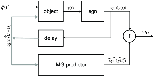
Figure 1: Block scheme presents the MG in the configuration of prediction.

The delay block introduces a one-step delay to its every input sample $y(t)$ and forms the vector $\vec{y}(t-n)$ of $n>1$ past samples. The MG model predicts the next sign of sample exploiting the information included in the signs of previous movements. The block $f$ compares the predicted signal with a real output of the object and calculates the correctness $\Psi(t)$. The correctness $\Psi(t)$ represents the average success rate of prediction and is calculated as a percentage of properly predicted signs of $y$, provided that all samples up to time $t$ are considered:

$$\Psi(t)=\frac{1}{t}\sum_{n=1}^{t}\delta(\mbox{sgn}(y(n)),\widehat{\mbox{sgn}(y(n))})$$ (6)

where $\delta$ stands for Kronecker symbol.

Two types of objects were analyzed: the autoregressive stochastic processes and the time series of real prices of shares. The former is mainly used to demonstrate interesting properties of the model and to learn how to tune its parameters. The latter one is used as an example of practical application of the predictor. In the case of the autoregressive stochastic process, assuming that the definition of the object is known, the maximal theoretical level of $\Psi$ can be calculated as follows:

$$\Psi^{MAX}(t)=\frac{1}{t}\sum_{n=1}^{t}\delta(\mbox{sgn}(y(n)),\mbox{sgn}({\mathbb{E}}[y(n)])).$$ (7)

The expected value ${\mathbb{E}}[y(n)]$ is calculated recursively for each $n$ according to the process definition.

5 Optimization of the parameters

Initially, we apply the predictor to the third order autoregressive time series, AR(3) defined as follows:

$$y(t)=0.7y(t-1)-0.5y(t-2)-0.2y(t-3)+\xi(t),$$ (8)

where $\xi(t)$ is an instance of the standardized gaussian white noise. It is easy to check that the process is stable. It was found numerically that the process is characterized by ${\mathbb{E}}[\Psi^{MAX}]=0.77$, and ${\mathbb{V}ar}[\Psi^{MAX}]<0.01$, where $t=3000$ steps, and the average was taken over ten realizations.

5.1 Majority vs minority game

The model extensively used in literature is based on the grand canonical minority game  [17, 15, 13, 14, 10]. However, it was not obvious for us if the minority mechanism is better than the majority one. In fact we found that, in the case of prediction, both mechanisms are equivalent.

The algorithm of the majority game is very similar to that of the standard minority game. The only difference is a formula (4) which for majority game reads

$$\Phi_{\alpha_{n}^{s}}(t)=a_{\alpha_{n}^{s}}(t)\,g[A(t)].$$ (9)

We consider two time series: the endogenous and exogenous. Considering first the game with endogenous time series we find a number of differences between the minority and majority game. In the minority game no one of strategies is permanently profitable provided that the game is large enough [16, 25]. Hence, the number of winners and losers changes in time. On the contrary, in the majority game the number of winners and losers is stable and, on average, $N(1-\frac{1}{2^{S}})$ agents are in majority. The reasoning behind is similar to that presented in Refs. [23, 24] and utilizes our observation that the first large oscillation creates a comprehensive difference in utilities of strategies. The strategies are divided into two categories: the good with the positive payoff, and bad ones with negative. In any time step $t$ there is on average $N(1-\frac{1}{2^{S}})$ agents with at least one good strategy and only $N/2^{S}$ agents with all bad strategies. Since most of agents has at least one good strategy - they use it. The difference, compared to the minority game, is that those who are in majority are not interested in changing the choice when they win. Similarly, the losers cannot change their situation because they do not have even one good strategy. Given this, the division between these two groups stays stable and the aggregate demand and utilities exhibit the one-directional trend. It persists in contradiction to the minority game, where the processes are mean-reverting. The above is true if the payoff is linear and the feedback effect is incorporated, i.e. the series of decisions is endogenous. The reasoning is slightly modified when the step-like payoff is applied but also in this case the essential differences between the minority and majority game remain.

Intriguingly, both games are equivalent, regardless of the payoff, when series of decisions is exogenous. Originally, in the standard minority game, strategies predicting sign opposite to $y(t)$ are rewarded. Assuming that patterns in the exogenous signal exist, the individuals prefer more often strategies predicting $\mbox{sgn}(y(t))$ incorrectly i.e. most of them fail with prediction. The predictor aggregates decisions of individuals and acts in opposition to the majority, and, predicts correctly. Contrary to the minority game, in the majority game, strategies that correctly forecast $\mbox{sgn}(y(t))$ are rewarded and most of agents follow strategies more frequently recognizing patterns. Subsequently, the predictor acts according to action suggesting the majority and also correctly recognizes patterns. Given this, the majority and minority game should provide the same quality of prediction. This is confirmed by numerical simulations presented in Fig. 2 (right). The experiment was performed using ten realizations of the AR(3) process. The number of strategies per agent $S$ was set to $2$, the memory length $m$ to $3$ and the number of agents $N$ was varied. Two curves show the success rate of prediction related to the minority nad majority approaches. As it is seen, there are no qualitative differences between them. Small distortions are due to random choice of strategies at the beginning of all simulations.

5.2 Tuning of $m$, $N$ and $S$ parameters

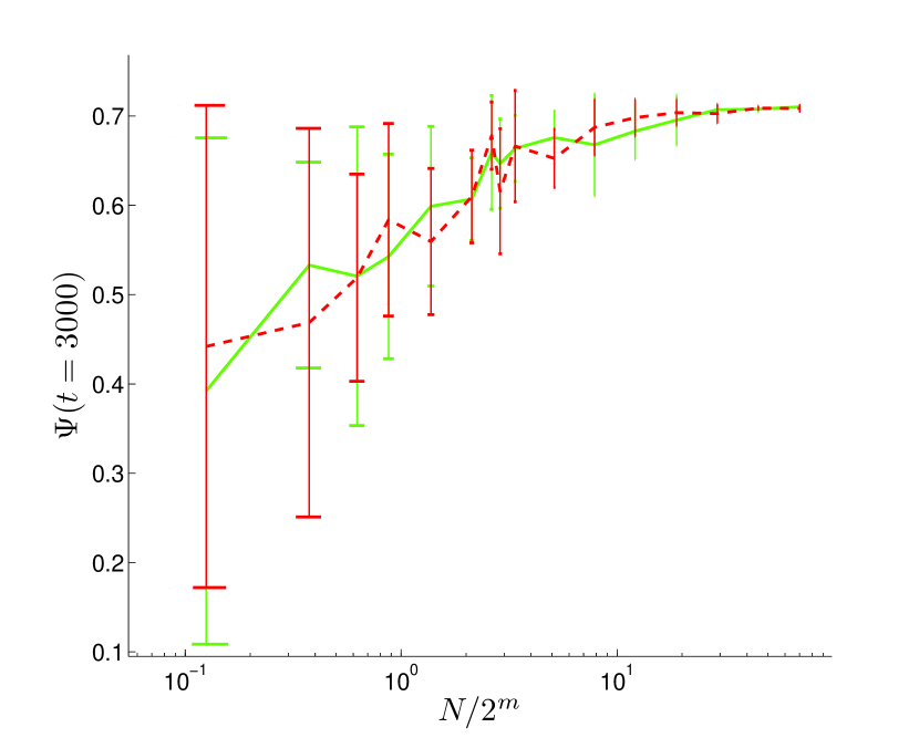
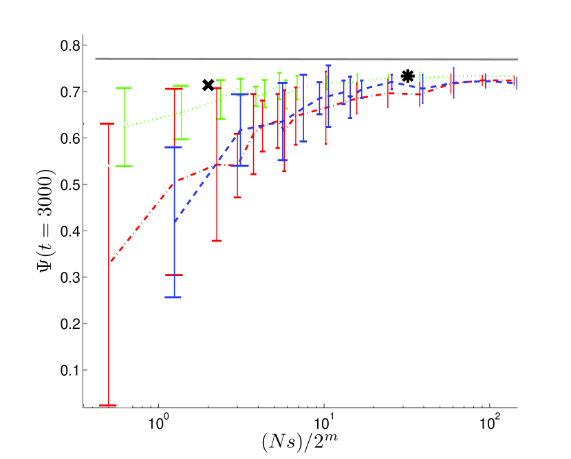
Figure 2: Left: Comparison of correctness $\Psi$ for the minority and majority games for $S=2$ and variable $N$. Red dashed line corresponds to the minority game and green solid line to the majority game. Right: Solid grey line corresponds to the theoretical maximal value, green dotted line corresponds to MG for $N=1$ and various $S$ values, blue dashed line corresponds to MG for $S=5$ and various $N$ values, red dash-dotted line corresponds to MG for $S=2$ and various $N$ values. The ’x’ mark corresponds to MG for $N=1$ and $S=16$ pairwise different strategies from the Reduced Strategy Space.The star ’*’ corresponds to MG for $N=1$ and $S=256$ pairwise different strategies from the Full Strategy Space. Error bars correspond to one standard deviation and curves are drawn to guide ones eye.

Considering three parameters: $m$,$N$ and $S$, at least $m$ requires different optimization techniques than two others. The optimization of $m$ is strictly related to analysis of time series properties, especially the analysis of the range of dependencies between values of $Y$. Therefore it depends on the researcher’s knowledge about the object. There are different methods of finding this range.

If the process is explicitly known, $m$ is equal to the order of this process, e.g. $m=3$ for AR(3). The predictor with $m$ lower than the order cannot work effectively because strategies would incorrectly recognize patterns. Larger values of $m$ would introduce additional and unnecessary noise that would degrade the prediction. The latter effect is further illustrated and explained in the section  6.2.

If the order is unknown but the type of the process is known (e.g. autoregressive one) some techniques based on the autocorrelation analysis can be applied to detect the order, as presented in Ref. [2].

The problem is most difficult if the order and the system are unknown, as it is in many real cases (e.g. prices in financial markets). Still the correlation analysis can suggest the number of past samples be used. In this section we assume that the order of the examined AR process is explicitly given.

In order to find the proper technique for $N$ and $S$ optimization, let us assume that a certain pool of strategies of constant size has to be optimally assigned to agents. It means that, under the constraint $NS=const$, we are looking for the proportion between number of agents $N$ and number of strategies per agent $S$ that maximizes the correctness $\Psi$. We would also like to examine if the optimal proportion is sensitive to the constraint’s change. Our numerical studies are presented in Fig. 2. The correctness is presented as a function of $NS$, as changing the size of the strategies’ pool influences the results. Solid grey line corresponds to the maximal value that is reached by the best possible predictor (in this case linear filter). Blue dashed line corresponds to MG for $S=5$ and various $N$ values, red dash-dotted line corresponds to MG for $S=2$ and various $N$ values. These two curves show that the more strategies per agent the better the correctness $\Psi$, provided that the constraint $NS=const$ is preserved. Following further this reasoning, the most efficient is obtained for just one agent possessing given pool of strategies. Indeed, this is confirmed by the green dotted line corresponding to MG for $N=1$ and various $S$ values. As it is seen, the predictor with such configuration outperforms any other predictor.

In order to reason out of the presented results, assume there are many agents but only one of them has the best strategy. Even if this strategy suggests a correct prediction for itself the prediction of the whole system can be potentially incorrect, provided there is sufficiently many agents with bad strategies. Such situation is less probable when the number of strategies per agent is increased and concurrently the number of agents is decreased. This is impossible if there is only one agent because then the best strategy is always used. Similarly, if the constraint on $NS$ is shifted towards larger values and number of agents is preserved, then the probability, that more and more agents have a correct strategy becomes large. Hence, in the limit $NS\rightarrow\infty$, all agents have the correct strategy and the efficiency of the group is the same as the efficiency of a single agent equipped with the aggregated pool of strategies.

Considering $\Psi$ as a function of the $S$ value, the larger value of $S$, the better results, as there is a larger probability that better strategy is drawn by an agent. However, if $S$ is above some threshold, the pool of strategies is oversampled and many agent’s strategies are the same. Since there is no particular gain if agent has more than one best strategy at his disposal, the success rate does not increase. Given this, one can wonder if a random draw is the most efficient way to generate strategies. Indeed it is not. Only the fully probed strategy space assures that, if the best strategy exists, then it is used in the game, provided $N=1$. The fringe benefit is that there is also no redundancy between strategies, what reduces the computational costs. Hence, the best MG predictor is based on single agent equipped with all pairwise different strategies, i.e. all strategies covering Full Strategy Space (FSS). However, in cases when $m$ is large, it can be hardly possible to generate so huge set of strategies. Therefore, for higher $m$ it seems reasonable to use all strategies from Reduced Strategy Space (RSS). The RSS consists of only $2^{m+1}$ strategies which are pairwise uncorrelated or anticorrelated, i.e. the normalized Hamming distance between them is equal to $0.5$ or $1$ [9]. The RSS apparently reduces the complexity and still assures good quality of prediction as FSS is regularly probed. These statements are visualized in Fig. 2 where marks ’x’ and ’*’ represent results for single agent and all strategies related to RSS (16 strategies) and FSS (256 strategies) respectively. Despite of a numerous differences between both pools the results are close, which indicates a superior power of RSS usage.

The presented above methodology differs significantly from approaches presented by other researchers [17, 13, 10]. In those papers the whole bunch of individuals is used and the strategy distribution is randomly initiated. Although those methods work either, the approach presented here is optimal.

5.3 Nonstationary signals and $\lambda$-GCMG predictor

The agents’ behavior is determined by the strategies’ utilities which they have at their disposal. Generally, the strategies that collect more frequently a positive payoff are characterized by a monotonously rising utilities. The utilities are thus potentially unbounded, what carries some considerable consequences if the exogenous process is a non-stationary one. Namely, if characteristics of a modelled object changes at time $t$ then the group of best strategies would change either. But if, until $t$, some strategies collected many positive payoffs and after time $t$ they are no longer profitable, then many steps with negative payoffs are required to lower their utilities. Hence, after time $t$ the system still uses potentially ineffective strategies. The following example should provide some deeper understanding of this issue.

Let us assume that after 1500 steps the system described by Eq. 8 is replaced by the following one: $y(t)=-0.3y(t-1)-0.2y(t-2)+0.6y(t-3)+\xi(t)$. The new $AR(3)$ process is defined in such a way that the best MG strategies for this process constitute also the set of the worst strategies of the previous process. Trajectories of utilities of GCMG predictor are in Fig. 3.

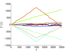
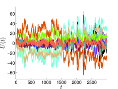
Figure 3: U(t) of all sixteenth pairwise different strategies from RSS for MG characterized by $N=1$ and $m=3$. The first figure corresponds to a classical GCMG. The second figure corresponds to the modified $\lambda$-GCMG with $\lambda=0.97$.

One can see that after time $t=1500$ the predictor still uses strategy which is no longer efficient, but is characterized by the highest $U$. As a result, the $\Psi$ as a function of time starts to decrease, as seen in Fig.5 (green dotted line).

In order to speed up the new appraisal of outdated $U$ we modified the predictor by introducing additional parameter $\lambda$ to the rule (5) that now is as follows.

$$U_{\alpha_{n}}(t+1)=\lambda U_{\alpha_{n}}(t)+\Phi_{\alpha_{n}}(t),$$ (10)

where $\lambda\in[0,1]$. If $\lambda=1$ the strategies have an infinite memory of all previous rewards, what corresponds to standard MG. If $\lambda=0$, then there is no memory effect and the best strategy is the one with the largest payoff in the previous step. The intermediate values $0<\lambda<1$ preserve increasing of $U$ to infinity, when the process is a stationary one, what considerably speeds up the time of adaptation. The exemplified results for the GCMG with $\lambda=0.97$ are presented in Fig. 3 (right). All initial conditions are the same as for picture in the left. It is seen that for $t>1500$ the new best strategy achieves the largest $U$ much faster than the game without $\lambda$ modification. The system is able to quickly adjust to changes, and the success rate of prediction is significantly improved, as presented in Fig. 5.

The cost of the introduction of the additional parameter is a need of its optimization. The heuristic analysis of correctness as a function of $\lambda$ is presented in Fig. 5. The value $\lambda=0.97$ assures the best results, although other values, that are close to it, work effectively either.

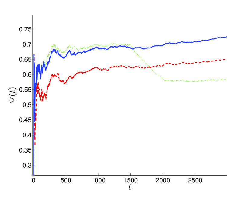
Figure 4: The time evolution of $\Psi(t)$ for $\lambda$-GCMG with $N=1$ and $S=16$ pairwise different strategies from RSS. Red dashed line corresponds to $\lambda=0.7$, solid blue line corresponds to $\lambda=0.97$ , green dotted line corresponds to $\lambda=1$.

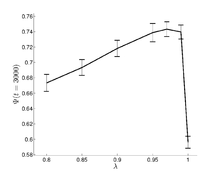
Figure 5: The $\Psi(t)$ at time $t=3000$ for $\lambda$-GCMG with $N=1$, $S=16$ pairwise different strategies from RSS and $\lambda=0.97$. Error bars correspond to one standard deviation and curves are drawn to guide ones eye. Statistics are calculated over 10 realizations of nonstationary AR(3) process.

Summing up, the $\lambda$-GCMG model effectively follows changes in the predicted signal and significantly outperforms the GCMG for a non-stationary process.

6 Sign prediction of assets’ returns

In this section we present the assumed model of movements of share prices. Given this we apply the $\lambda$-GCMG predictor to retrieve dependencies between past and future samples of stocks prices taken from various markets.

6.1 Price movements model

We assume that, generally, the dynamics of returns is driven by two factors where one is endogenous and another one exogenous. The model of return rate is

$$r(t)=f[r(t-1),\ldots,r(t-m)]+\xi(t),$$ (11)

where the first term reflects a dependence on previous returns and the second term represents the influence of external events.

To be precise, because MG predicts only the sign and not a value of sample, we have to assume even stronger:

$$\mbox{sgn(r(t))}=f[\mbox{sgn}\ r(t-1),\ldots,\mbox{sgn}\ r(t-m)]+\xi(t).$$ (12)

We assume that the exact form of function $f$ is unknown and it can evolve over time. In case of the model in Fig. 1, the returns $r(t)$ correspond to signals $y(t)$.

Considering the second term $\xi(t)$, there are many various exogenous factors, e.g. publication of the Gross Domestic Product, inflation, companies annual balances, bankruptcies, etc. Investors react on them in various ways. Therefore, instead of considering reactions of individuals separately, we assume that signals of $\xi(t)$ are instances of IID process, with mean value equal to zero. This signal aggregates reactions of all individuals on all news that appear at time $t$. Such an approach significantly simplifies further analysis, sice we have to pay an attention only to dependencies between past and future returns and not to such relations between exogenous factors.

The assumption that exogenous perturbations to returns are IID variables seems more reasonable in the case of intraday data than for the end-of-day data. As mentioned in the paper [17], exogenous events are relatively infrequent compared to the typical transaction rate in the markets. This suggests that the majority in high-frequency data movements can be potentially self-generated, while the lower frequencies are dominated by exogenous factors.

6.2 Application of $\lambda$-GCMG

We look for a $\lambda$-GCMG model being able to estimate function $f$ in Eq. (12). Using our previous results, we set the following parameter values: $N=1$, $\lambda=0.97$ and the number of strategies covering the RSS. The $m$ value should be chosen from the range $1-10$. This premise is given by the analysis of data from the London Stock Exchange (LSE) presented in Refs. [1, 20, 12]. The precise choice of $m$ requires some additional analysis. If we take a look at Fig. 6, where the $\lambda$-GCMG is applied as a predictor to FW20 time series i.e. futures contracts on WIG20 index that is the index of the twenty largest companies on the Warsaw Stock Exchange, then it is seen that better correctness is achieved for lower $m$ i.e. $m=1$.

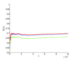
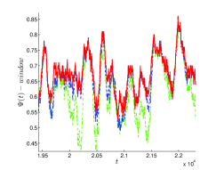
Figure 6: The time evolution of $\Psi(t)$ (left) and $\Psi(t)$ calculated in sliding window of length equal to $100$ (right) for $\lambda$-GCMG with $N=1$, $\lambda=0.97$ and strategies from Reduced Strategy Space. Red solid line corresponds to $m=1$, dashed blue line corresponds to $m=2$ , green dashed-dotted line corresponds to $m=5$ (left). The predicted signal is FW20.

This result, at least at first sight, seems to be counter-intuitive. The RSS of higher order includes all strategies of RSS of lower order and additionally introduces the same number of extra strategies. For example, if $m=2$ then 4 of 8 strategies recognize the same patterns as strategies for $m=1$ and additional 4 strategies introduce new functionality. The explanation is that for higher $m$ the additional strategies, although do not capture properly dependencies, get from time to time higher utility than the basic ones correctly recognizing shorter patterns. This happens randomly, as sometimes samples are in order that is reflected by some of additional strategies. However, the pattern does not truly exist. In the next steps the forecast, based on one of additional strategies, is mostly wrong, what lowers the correctness. In other words, too long memory spoils the predictor introducing noise of unwanted strategies. The more the memory length $m$ exceeds real order of the system, the lower the success rate of prediction. The observed degradation of correctness for longer $m$ indicates that there are no long-range and complicated patterns in the signal or that their nature is more subtle than MG strategies are able to capture. The first statement is supported by observations of the autocorrelation of returns, where the only distinct value is for $\tau=1$. Similar premise is also included in Ref. [18] where the author found that strategies with shorter $m$ are more preferred by individuals.

The success rate for $m=1$, it is mostly above $0.6$, and from time to time even touches the level $0.8$, if calculated in the sliding window. The mean value of correctness is $0.7$ (see Fig. 6 - left), what seems impressive, at the first sight. However, we checked that the correctness of Finite Impulse Response (FIR) Wiener filter [3] of the first order is equal to $0.68$. The use of higher-order filters does not improve the predictor and, at least in this case, the linear regression is good enough to assure similar results.

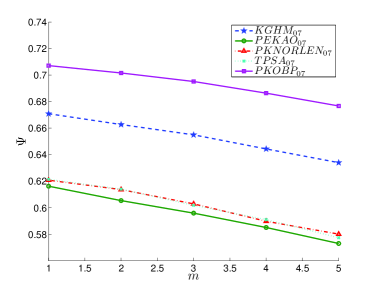
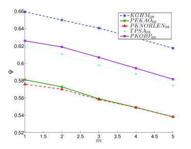
Figure 7: The correctness $\Psi$ as a function of the memory length $m$, for 5 companies with the biggest impact on index WIG20 for two different years 2007 (left) and 2008 (right).

The next question is, whether the results achieved for FW20 are specific only for this asset or they are more universal. We examined separately 5 stocks with the biggest impact on FW20 index: PKNORLEN, PEKAO, KGHM, PKOBP, TPSA, each of them contributing to the index at the level of $11-14\%$. As seen in Fig. 6, the success rate decreases as a function of $m$, regardless of the analyzed year. So the results seem to be time and stock independent.

Another interesting issue is related to the analysis of the best strategy. The question is, whether there is only one strategy permanently outperforming other strategies or, maybe, different strategies lead at various moments? If there is only one, it would mean that patterns do not change over the game or that they do in a way the strategies are unable to capture. One permanently best strategy also would mean that the extended adaptive version of algorithm is, at least in this case, as good as an ordinary GCMG or even as good as a linear filter. Indeed, in Fig. 8 (left) it is seen that one of the strategies permanently outperforms others. Interestingly, this strategy represents the mean-reverting approach, i.e. after history $\mu=1$ it suggests $a=-1$ and after $\mu=-1$ it suggests $a=1$. Accordingly, the opposite strategy representing a trend-follower approach, is the worst one. The results are consistent with autocorrelation analysis where for $\tau=1$ the coefficient is negative. We checked that the results are general for all five examined firms.

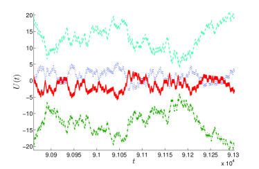
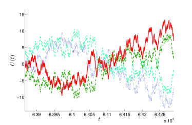
Figure 8: The time evolution of $U(t)$ for all of 4 strategies for $\lambda$-GCMG with $N=1$ and $\lambda=0.97$ for index FW20 (left) and Astrazenca company (right).

The results for Polish market cannot be easily generalized to the London Stock Exchange market. For example, companies like Vodafone or Astrazeneca are not characterized by only one strategy being permanently better than others (cf. Fig. 8 - right). The more so, for Astrazeneca, the best results with the correctness equal to $0.6$ are achieved for $m=2$. It is difficult to explain why such fundamental differences between stock markets exist. One of the hypotheses is that the Polish market is less mature than LSE and dependencies between samples are stronger. Although the hypothesis partially explains the larger values of autocorrelations for $\tau=1$ in Polish market, it does not explain the longer ranges of the LSE autocorrelations. This remains an open question.

The above analysis also shows that it is difficult to build a profitable investing system if one would capture patterns using only agents’ strategies. If a sign of a next increment is known to the investor with encouraging probability, then the investor has to put the order. But placing the order introduces a perturbation to the forecast. If the order is executed, the system would move to the next time step and the transaction would be considered as entailing the positive or negative increment. The investor would predict only its own transactions what, of course, does not assure any profit. Given this, the prediction for at least two steps is required.

7 Conclusion

We applied the minority game as a predictor of an exogenous process. Interestingly, considering parameters’ optimization, we found that the degenerated game with only single agent and all strategies from FSS is the most efficient configuration. The reason behind is as follows. The FSS is accessible to every agent and all agents can use all possible patterns. Since there is only one agent, there is no decision noise from other, badly equipped agents. If using the FSS is computationally impossible, then the RSS is recommended. Considering the quality of prediction, minority and majority games are equivalent. Considering non-stationary signals, the parameter $\lambda$ is introduced in order to speed up the model’s convergence. However, the additional parameter requires extra optimization. This parameter is introduced on heuristic basis.

Applying the predictor to the intraday financial time series allows to effectively perform for one step where the correctness reaches $70\%$ of properly recognized signs. The best strategy in the case of Polish stocks is a mean-reverting one. Only slightly worse predictions are attained by autoregressive systems. Unfortunately, these encouraging results are mostly useless, for building a profitable investing system. We explained that successful acting requires statistically significant forecasts for more than only one step forward. The values of autocorrelation function for $\tau>1$ suggest that it is hard to achieve. Nevertheless, the complexity of human and algorithmic actions reflecting price movements consist surely of nonlinear dependencies not properly captured in the autocorrelation analysis. Therefore, application of MG to the prediction of longer periods seems to be worth to check. The more so, the idea of building a profitable investing system requires, in most cases, not only the knowledge of the direction of the price movement but also some information about the strength of it. Hence, the additional statistical methods should be compounded with the MG-predictor in order to invest effectively. We consider it as a next step in our research.

References

- [1] J.P. Bouchaud, Y. Gefen, M. Potters, and M. Wyart. Fluctuations and response in financial markets: the subtle nature of ‘random’ price changes. In Quantitative Finance, volume 4, pages 176 – 190, 2003.
- [2] G. Box, G. M. Jenkins, and G. Reinsel. Time Series Analysis: Forecasting & Control. Prentice Hall; 3rd edition, 1994.
- [3] R.G. Brown and P.Y.C. Hwang. Introduction to Random Signals and Applied Kalman Filtering with Matlab Exercises and Solutions, 3rd Edition. John Wiley & Sons, INC., 1997.
- [4] A. Cavagna. Irrelevance of memory in the minority game. In Physical Review E, volume 59, pages R3783 – R3786, 1999.
- [5] D. Challet and M. Marsili. Phase transition and symmetry breaking in the minority game. In Physical Review E, volume 60, pages 6271 – 6274, 1999.
- [6] D. Challet and M. Marsili. Relevance of memory in minority games. In Physical Review E, volume 62, pages 1862 – 1868, 2000.
- [7] D. Challet, M. Marsili, and Y.C.Zhang. Modeling market mechanism with minority game. In Physica A, volume 276, pages 284 – 315, 2000.
- [8] D. Challet and Y.C. Zhang. Emergence of cooperation and organization in an evolutionary game. In Physica A, volume 246, pages 407 – 418, 1997.
- [9] D. Challet and Y.C. Zhang. On the minority game: Analytical and numerical studies. In Physica A, volume 256, pages 514 – 532, 1998.
- [10] F. Chen, C. Gou, X. Guo, and J. Gao. Prediction of stock markets by the evolutionary mix-game model. In Physica A, volume 387, pages 3594 – 3604, 2008.
- [11] A.C.C. Coolen. The mathematical theory of minority games: statistical mechanics of interacting agents. Oxford Unversity Press, 2005.
- [12] A.N. Gerig. A theory for market impact: How order flow affects stock price. PhD dissertation, University of Illinois, 2007.
- [13] C. Gou. Predictability of Shanghai Stock Market by agent-based mix-game model. In Proceeding of IEEE ICNN&B 05, pages 1651 – 1655, 2005.
- [14] Chengling Gou. Dynamic behaviors of mix-game models and its application. In Chinese Physics, volume 15, page 1239, 2006.
- [15] P. Jefferies, M.L. Hart, P.M. Hui, and N.F. Johnson. From market games to real-world markets. In The European Physical Journal B, volume 20, pages 493 – 501, 2001.
- [16] N. F. Johnson, M. Hart, and P.M. Hui. Crowd effects and volatility in in markets with competing agents. In Physica A, volume 269, pages 1 – 8, 1999.
- [17] N.F. Johnson, D. Lamper, P. Jefferies, M.L. Hart, and S. Howison. Application of multi-agent games to the prediction of financial time series. In Physica A, volume 299, pages 222 – 227, 2001.
- [18] A. Krause. Evaluating the performance of adapting trading strategies with different memory lengths. In Proceeding of IDEAL 2009, pages 711 – 718, 2009.
- [19] C.Y. Lee. Is memory in the minority game irrelevant? In Physical Review E, volume 65, page 015102, 2001.
- [20] F. Lillo and J.D. Farmer. The long memory of the efficient market. In Studies in Nonlinear Dynamics & Econometrics, volume 8, pages 1 – 33, 2004.
- [21] E. Moro. The minority game: an introductory guide. In Advances in Condensed Matter and Statistical Physics, pages 263 – 286. Nova Science Publishers, Inc., 2004.
- [22] R. Savit, R. Manuca, and R. Riolo. Adaptive competition, market efficiency, and phase transitions. In Physical Review Letters, volume 82, pages 2203 – 2206, 1999.
- [23] K. Wawrzyniak and W. Wiślicki. Multi-market minority game: breaking the symmetry of choice. In Advances in Complex Systems, volume 12, pages 423 – 437, 2009.
- [24] K. Wawrzyniak and W. Wiślicki. Phenomenology of minority games in efficient regime. In Advances in Complex Systems, volume 12, pages 619 – 639, 2009.
- [25] K. Wawrzyniak and W. Wiślicki. Mesoscopic approach to minority games in herd regime. In in preparation, volume tbd, page tbd, 2011.