Three-body model calculations for $N=Z$ odd-odd nuclei with $T=0$ and $T=1$ pairing correlations

Abstract

We study the interplay between the isoscalar ($T=0$) and isovector ($T=1$) pairing correlations in $N=Z$ odd-odd nuclei from ¹⁴N to ⁵⁸Cu by using three-body model calculations. The strong spin-triplet $T=0$ pairing correlation dominates in the ground state of ¹⁴N, ¹⁸F, ³⁰P, and ⁵⁸Cu with the spin-parity $J^{\pi}=1^{+}$, which can be well reproduced by the present calculations. The magnetic dipole and Gamow-Teller transitions are found to be strong in ¹⁸F and ⁴²Sc as a manifestation of SU(4) symmetry in the spin-isospin space. We also discuss the spin-quadrupole transitions in these nuclei.

I Introduction

The pairing correlation is one of the most remarkable effects in nuclear physics. It appears in many properties of nuclei, including odd-even mass staggering, as well as the large energy gap between the first excited and the ground states in even-even nuclei compered to odd-even nuclei. In literature, the spin-singlet $T=1$ pairing has been mainly discussed in nuclear physics, since the large spin-orbit splitting prevents to couple a spin-triplet ($T=0$, $S=1$) pair in the ground state Bertsch2012 ; Sagawa2013 . Another reason for this is that the large neutron-excess along the stability line of the nuclear chart suppresses the proton-neutron pairing. A recent availability of radioactive beams has opened up an opportunity to measure structure properties of unstable nuclei along the $N=Z$ line, strongly enhancing a possibility to measure new properties of nuclei such as pairing correlations related with the spin-triplet $T=0$ pairing. It is thus quite interesting and important to study the competition between the spin-singlet $T=1$ and the spin-triplet $T=0$ pairing interactions in odd-odd $N=Z$ nuclei and seek an experimental evidence for the competition in the spins of low-lying states. In this paper, we focus our study in $sd$- and $pf$- shell nuclei, in which the ground state spins and spin-isospin transitions are observed. In order to study the ground state and the low-lying excited states in odd-odd $N=Z$ nuclei in these mass regions, we apply a three-body model with a density-dependent contact interaction between the valence neutron and proton.

The paper is organized as follows. In Sec. II, we explain the three-body model employed in the present study. In Sec. III, we present the results of the calculations and discuss the ground state properties of odd-odd $N=Z$ nuclei. We also discuss the magnetic moments, the magnetic dipole transitions, the isovector spin-quadrupole transitions, and the Gamow-Teller transitions in these nuclei. We summarize the paper in Sec. IV.

II Model

We first describe the model Hamiltonian for $N=Z$ nuclei, assuming the core+ $p+n$ structure Tanimura12 . This model is based on the three-body model for describing the properties of Borromean nuclei such as ¹¹Li and ⁶He BeEs91 ; EsBeH97 ; HS2005 . In the rest frame of the three-body system, the model Hamiltonian is given by

$$H = \frac{\mbox{\boldmath$p$}_{p}^{2}}{2m}+\frac{\mbox{\boldmath$p$}_{n}^{2}}{2m}+V_{pC}(\mbox{\boldmath$r$}_{p})+V_{nC}(\mbox{\boldmath$r$}_{n})$$ (1)

$$+V_{pn}(\mbox{\boldmath$r$}_{p},\mbox{\boldmath$r$}_{n})+\frac{(\mbox{\boldmath$p$}_{p}+\mbox{\boldmath$p$}_{n})^{2}}{2A_{C}m},$$

where $m$ is the nucleon mass and $A_{C}$ is the mass number of the core nucleus. $V_{pC}$ and $V_{nC}$ are the mean field potentials for the valence proton and neutron, respectively, generated by the core nucleus. These are given as

$$V_{nC}(\mbox{\boldmath$r$}_{n})(r)=V^{(N)}(r_{n}),\ V_{pC}(\mbox{\boldmath$r$}_{p})=V^{(N)}(r_{p})+V^{(C)}(r_{p}),$$ (2)

where $V^{(N)}$ and $V^{(C)}$ are the nuclear and the Coulomb parts, respectively. In Eq. (1), $V_{pn}$ is the pairing interaction between the two valence nucleons. For simplicity, we neglect in this paper the recoil kinetic energy of the core nucleus, that is, the last term in Eq. (1).

The nuclear part of the core-valence particle interaction, Eq. (2), is taken to be

$$V^{(N)}=v_{0}f(r)+v_{ls}\frac{1}{r}\frac{df(r)}{dr}(\mbox{\boldmath$l$}\cdot\mbox{\boldmath$s$}),$$ (3)

where $f(r)$ is a Fermi function defined by $f(r)=1/(1+\exp[(r-R)/a])$. For ¹⁸F nucleus, as in Ref. Tanimura12 , we set $v_{0}=-49.21$ MeV and $v_{ls}=21.6$ MeV$\cdot$fm². For the other nuclei, we adjust $v_{0}$ so as to reproduce the neutron separation energies, while $v_{ls}$ is kept constant for all the nuclei considered in this paper. The radius and the diffuseness parameters are set to be $R=1.27A_{C}^{1/3}$ fm and $a=0.67$ fm, respectively. The Coulomb potential $V^{(C)}$ in the proton mean field potential is generated by a uniformly charged sphere of radius $R$ and charge $Z_{C}e$, where $Z_{C}$ is the atomic number of the core nucleus. We use a contact interaction between the valence neutron and proton, $V_{np}$, given asTanimura12 ,

$$V_{np}(\mbox{\boldmath$r$}_{1},\mbox{\boldmath$r$}_{2}) = \hat{P_{s}}v_{s}\delta(\mbox{\boldmath$r$}_{1}-\mbox{\boldmath$r$}_{2})\left[1+x_{s}\left(\frac{\rho(r)}{\rho_{0}}\right)^{\alpha}\right]$$ (4)

$$+\hat{P_{t}}v_{t}\delta(\mbox{\boldmath$r$}_{1}-\mbox{\boldmath$r$}_{2})\left[1+x_{t}\left(\frac{\rho(r)}{\rho_{0}}\right)^{\alpha}\right],$$

where $\hat{P}_{s}$ and $\hat{P}_{t}$ are the projectors onto the spin-singlet and spin-triplet channels, respectively:

$$\hat{P}_{s}=\frac{1}{4}-\frac{1}{4}{\boldsymbol{\sigma}}_{p}\cdot{\boldsymbol{\sigma}}_{n},\ \hat{P}_{t}=\frac{3}{4}+\frac{1}{4}{\boldsymbol{\sigma}}_{p}\cdot{\boldsymbol{\sigma}}_{n}.$$ (5)

In each channel in Eq. (4), the first term corresponds to the interaction in vacuum while the second term takes into account the medium effect through the density dependence. Here, the core density is assumed to be a Fermi distribution of the same radius and diffuseness as in the core-valence particle interaction, Eq. (3). The strength parameters, $v_{s}$ and $v_{t}$, are determined from the proton-neutron scattering length as EsBeH97

$$v_{s} = \frac{2\pi^{2}\hbar^{2}}{m}\frac{2a^{(s)}_{pn}}{\pi-2a^{(s)}_{pn}k_{\rm cut}},$$ (6)

$$v_{t} = \frac{2\pi^{2}\hbar^{2}}{m}\frac{2a^{(t)}_{pn}}{\pi-2a^{(t)}_{pn}k_{\rm cut}},$$ (7)

where $a^{(s)}_{pn}=-23.749$ fm and $a^{(t)}_{pn}=5.424$ fm KoNi75 are the empirical p-n scattering lengths in the spin-singlet and spin-triplet channels, respectively. $k_{\rm cut}$ is the momentum cut-off introduced in treating the delta function, which is related with the cutoff energy as $E_{\rm cut}=\hbar^{2}k_{cut}^{2}/m.$ The strengths $v_{s}$ and $v_{t}$ determined from the scattering lengths depend on the cutoff energy, $E_{\rm cut}$, as will be discussed in Sec. III. The three parameters $x_{s},\ x_{t}$, and $\alpha$ in the density-dependent terms in Eq. (4) are determined so as to reproduce energies of the ground ($J^{\pi}=1^{+}$), the first excited ($J^{\pi}=3^{+}$), and the second excited ($J^{\pi}=0^{+}$) states in ¹⁸F with respect to the three-body threashold (See also Ref. Tanimura12 ). The density $\rho(r)/\rho_{0}$ is replaced by a Fermi function $f(r)$ hereafter.

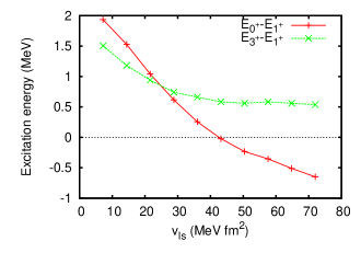
Figure 1: (Color online) The excitation energies of the first 0${}^{+}_{1}$ and the first 3${}^{+}_{1}$ states in ¹⁸F obtained with the three-body model as a function of the spin-orbit strength $v_{ls}$ in the mean-field potential. The excitation energies are measured from the energy of the first 1${}^{+}_{1}$ state.

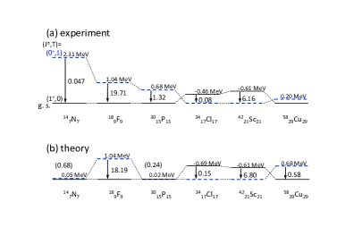
Figure 2: (Color online) The energies of the first 0${}^{+}_{1}$ and the first 1${}^{+}_{1}$ states in $N=Z$ nuclei. The upper panel (a) shows experimental data and the lower panel (b) corresponds to calculated results. The values with the arrows show the transition probabilities for the magnetic dipole transitions, $B(M1)$ (the calcurated values are shown in the brakets for ¹⁴N and ³⁰P). The experimental data are taken from Ref. exp .

The Hamiltonian (1) is diagonalized in the valence two-particle model space. The basis states for this are given by a product of proton and neutron single particle states with the single particle energy $\epsilon^{(\tau)}$, which are obtained with the single-particle potential $V_{\tau C}$ in Eq. (1) ($\tau=p$ or $n$). To this end, the single-particle continuum states are discreized in a large box. We include only those states satisfying $\epsilon^{(p)}_{\alpha}+\epsilon^{(n)}_{\beta}\leq E_{\rm cut}$. We use the proton-neutron formalism without antisymmetrization in order to take into account the breaking of the isospin symmetry due to the Coulomb interaction.

III Results

The spin-orbit potential in the mean-field potentials plays a crucial role in determining the properties of $T=0$ pairing as discussed in Refs. Bertsch2012 ; Poves98 ; Bertsch11 . In Fig. 1, we plot the energy differences between the first 0⁺ and 1⁺ states and between the first 3⁺ and 1⁺ states in ¹⁸F as a function of the spin-orbit coupling strength $v_{ls}$. We use the cutoff energy of $E_{\rm cut}=20$ MeV. It is clearly seen in Fig. 1 that the $T=0$ pairing correlations decreases as the spin-orbit interaction increases. That is, the energy difference $E_{0^{+}}-E_{1^{+}}$ decreases and eventually the spectrum is reversed so that the 0⁺ state becomes the ground state, where the $T=1$ pairing overcomes the $T=0$ pairing.

The calculated spectra for ¹⁴N, ¹⁸F, ³⁰P, ³⁴Cl, ⁴²Sc, and ⁵⁸Cu nuclei are shown in Fig. 2 together with the experimental data. The spin-parity for the ground state of the nuclei in Fig. 2 are $J^{\pi}=1^{+}$ except for ³⁴Cl and ⁴²Sc. This feature is entirely due to the interplay between the isoscalar spin-triplet and the isovector spin-singlet pairing interactions in these $N=Z$ nuclei. In the present calculations, the ratio between the isoscalar and the isovector pairing interactions is $v_{t}/v_{s}=1.9$ for the energy cutoff of the model space, $E_{\rm cut}=20$ MeV. This ratio is somewhat larger than the value $\sim$1.6 obtained in Ref. Bertsch11 from the shell model matrix elements in $p$- and $sd$-shell nuclei. For a larger model space with $E_{\rm cut}=30$ MeV, the ratio becomes 1.6, but the agreement between the experimental data and the calculations somewhat worsens quantitatively even though the general feature remains the same. It is remarkable that the energy differences $\Delta E=E(0^{+}_{1})-E(1^{+}_{1}$) are well reproduced in ³⁴Cl and ⁴²Sc both qualitatively (the inversion of the 1⁺ and 0⁺ states in the ground state) and quantitatively (the absolute value of the energy difference). The model description is somewhat poor in ¹⁴N and ³⁰P because the cores of these two nuclei are deformed, although the ordering of the two lowest levels are correctly reproduced.

The probability of the total spin $S=0$ and $S=1$ components for the $0^{+}$ and the 1⁺ states, respectively, are listed in Table LABEL:tab:1. The total spin $S=0$ and $S=1$ components in two particle configurations can be calculated with a formula

$$|(j_{\pi}j_{\nu})J\rangle=\sum_{L,S}\left\{\begin{array}[]{ccc}l_{\pi}&l_{\nu}&L\\ s&s&S\\ j_{\pi}&j_{\nu}&J\end{array}\right\}\hat{L}\hat{S}\hat{j_{\pi}}\hat{j_{\nu}}|(l_{\pi}l_{\nu})LS;J\rangle$$ (11)

with the $9j$ symbol and a factor $\hat{L}\equiv\sqrt{2L+1}$. For a $j_{\pi}=j_{\nu}=j=l+1/2$ configuration, the $S=0$ and $S=1$ components are given by the factors $(j+1/2)/2j$ and $(j-1/2)/2j$, respectively, for $J$=0. For a $j_{\pi}=j_{\nu}=j=l-1/2$ configuration, on the other hand, they are $(j+1/2)/(2j+2)$ and $(j+3/2)/(2j+2)$ for $S=0$ and $S=1$, respectively. Notice that $s_{1/2}^{2}$ configuration has only $S=0$ component if $J=0$. Otherwise, all the two particle states have a large mixture of the $S=0$ and $S=1$ components. In general, the $S=1$ and $S=0$ components are thus largely mixed in the wave functions of both the ground and the excited states. An exception is ³⁰P. In this nucleus, the dominant configuration in the 0⁺ state is $(2s_{1/2}^{\pi}\otimes 2s_{1/2}^{\nu})$, which can couple only to the total spin $S=0$. On the other hand, in the 1⁺ state, the dominant configuration is $(2s_{1/2}\otimes 1d_{3/2})~{}{T=0}$ which can couple only to the total spin $S=1$ with the total angular momentum $L=2$.

Table 1: The energy difference between the 0${}^{+}_{1}$ and $1^{+}_{1}$ states, $\Delta E=E(0^{+}_{1})-E(1^{+}_{1}$), in $N=Z$ nuclei. The probabilities of the $S=0$ component $P(S=0)$ in the wave functions for the $0_{1}^{+}$ state are shown in the fourth line. The fifth line shows the probability of the $S=1$ component in the 1⁺ state. The probabilities $P(j^{\pi}\otimes j^{\nu})$ for the dominant valence shell proton-neutron configuration are also given for the 0${}^{+}_{1}$ and 1${}^{+}_{1}$ states in the 7th and 8th lines, respectively. The experimental data is taken from Ref. exp .

		14N	18F	30P	34Cl	42Sc	58Cu
$\Delta E$	exp.	2.31	1.04	0.68	$-0.46$	$-0.61$	0.20
(MeV)	cal.	0.05	1.04	0.02	$-0.69$	$-0.61$	0.68
$P(S=0)$ (%)	$0^{+}$	34.8	82.2	94.8	40.7	70.5	65.4
$P(S=1)$ (%)	$1^{+}$	78.3	90.1	95.8	64.3	65.7	92.1
$j$		$1p_{1/2}$	$1d_{5/2}$	$2s_{1/2}$	$1d_{3/2}$	$1f_{7/2}$	$2p_{3/2}$
$P(j^{\pi}\otimes j^{\nu})$	$0^{+}$	97.2	85.2	89.7	98.6	94.2	81.2
(%)	$1^{+}$	96.4	52.1	1.1	98.4	82.7	10.0

We next discuss the magnetic moment for the $1^{+}$ state, and the magnetic dipole transition strength $B(M1)\downarrow$ and the isovector spin-quadrupole transition strength $B(IVSQ)\uparrow$ between $0^{+}_{1}$ and $1^{+}_{1}$ states. The symbol $\downarrow(\uparrow)$ means the transition from the excited (ground) to the ground (excited) states. The magnetic operator is defined as

$$\mu=\langle 1^{+}|\sum_{i}(g_{s}(i)\mbox{\boldmath$s$}_{i}+g_{l}(i)\mbox{\boldmath$l$}_{i})|1^{+}\rangle,$$ (13)

where $g_{s}(i)$ and $g_{l}(i)$ are the spin and the orbital $g$ factors, respectively. The reduced magnetic dipole transition probability is given by

$$B(M1:J_{i}\rightarrow J_{f})=$$

$$\left(\frac{3}{4\pi}\right)\frac{1}{2J_{i}+1}\left|\langle J_{f}||\sum_{i}(g_{s}(i)\mbox{\boldmath$s$}_{i}+g_{l}(i)\mbox{\boldmath$l$}_{i})||J_{i}\rangle\right|^{2},$$ (14)

where the double bar means the reduced matrix element in the spin space. We take the bare $g$ factors $g_{s}(\pi)=5.58$, $g_{s}(\nu)=-3.82$, $g_{l}(\pi)=1$, and $g_{l}(\nu)=0$ for the magnetic moment and the magnetic dipole transitions in the unit of the nuclear magneton $\mu_{N}=e\hbar/2mc$. The spin-quadrupole transition is defined by

$$B(IVSQ:J_{i}\rightarrow J_{f})=$$

$$\frac{1}{2J_{i}+1}\left|\langle J_{f}||\sum_{i}(\tau_{z}(i)r_{i}^{2}[\mbox{\boldmath$\sigma$}(i)Y_{2}(i)]^{(\lambda=1)})||J_{i}\rangle\right|^{2}.$$ (15)

The calculated magnetic moments and the magnetic dipole transitions are listed in Table LABEL:tab:2 together with the spin quadrupole transitions. The calculated magnetic moment in ¹⁴N reproduces well the observed one, while the agreement is worse in ⁵⁸Cu. This is due to the fact that the core of ⁵⁶Ni might be largely broken and the $f_{7/2}-$hole configuration is mixed in the ground state of ⁵⁸Cu  Honma2004 . The values for $B(M1)$ are also shown in Fig. 2. Very strong $B(M1)$ values are found both experimentally and theoretically in two of the $N=Z$ nuclei in Table LABEL:tab:2, that is, in ¹⁸F and ⁴²Sc. The $B(M1)$ value from 0⁺ to 1⁺ in ¹⁸F is the largest one so far observed in the entire region of nuclear chart. We notice that our three-body calculations provide remarkable agreements not only for these strong transitions in ¹⁸F and ⁴²Sc but also quenched transitions in the other $N=Z$ nuclei such as in ¹⁴N and ³⁴Cl.

Table 2: The magnetic moments $\mu$, the magnetic dipole transitions, and the isovector spin quadrupole transitions in the $N=Z$ nuclei. The experimental data of $B(M1)$ values are taken from Ref. exp , while the data for the magnetic moment are taken from Ref. mmdata . The symbol $\downarrow(\uparrow)$ means the transition from the excited (ground) to the ground (excited) states.

		14N	18F	30P	34Cl	42Sc	58Cu
$J^{\pi}_{gs}$		$1^{+}$	$1^{+}$	$1^{+}$	$0^{+}$	$0^{+}$	$1^{+}$
$\mu$ ($\mu_{N}$)	exp.	0.404	–	–	–	–	0.52
	cal.	0.379	0.834	0.318	0.426	0.686	0.283
$B({M}1)\downarrow$ ($\mu_{N}^{2}$)	exp.	0.047	19.71	1.32	0.08	6.16	–
	cal.	0.682	18.19	0.24	0.15	6.81	0.580
$B({SQ})\uparrow$ (fm4)	cal.	33.17	0.85	43.04	74.52	19.61	71.55

In the case of ¹⁸F, the $0^{+}$ and $1^{+}$ states are largely dominated by the $S=0$ and $S=1$ spin components, respectively, with the orbital angular momentum $l=2$ (see Table I). Therefore, the two states can be considered as members of SU(4) multiplet in the spin-isospin space. This is the main reason why the $B(M1)$ value is so large in this nucleus, since the spin-isospin operator $g_{s}^{IV}\mbox{\boldmath$s$}\tau_{z}$ connects between two states in the same SU(4) multiplet, that is, the transition is allowed, and the isovector $g-$ factor is the dominant term in Eq. (14) with $g_{s}^{IV}=(g_{s}(\nu)-g_{s}(\pi))/2=-4.70$. The configurations in ⁴²Sc are also similar to those in ¹⁸F in terms of SU(4) multiplets, although they are dominated by $l=3$ wave functions. For ¹⁴N and ³⁴Cl, the $B(M1)$ transitions do not acquire any enhancement, since the $S=0$ component in the $0^{+}$ state is suppressed due to the $j=l-1/2$ coupling (both the $0^{+}$ and $1^{+}$ states have very large $1p_{1/2}^{2}$ ($1d_{3/2}^{2}$) configurations in ¹⁴N (³⁴C).) These indications for the SU(4) symmetry in ¹⁸F and ⁴²Sc are consistent with the results obtained in Refs. HaBa89 ; VoOr93 ; IsWaBr95 . In nuclei ³⁰P and ⁵⁸Cu, the 1⁺ state is dominated by 1$d_{3/2}2s_{1/2}$ and $2p_{3/2}1f_{5/2}$ configurations, respectively, while the 0⁺ state is governed by the $2s_{1/2}^{2}$ and $2p_{3/2}^{2}$ configurations, respectively. Therefore the isovector spin-quadrupole transitions are largely enhanced in the two nuclei even though the $B(M1)$ is much quenched.

We also calculate the Gamow-Teller (GT) strength

$$B(GT:0^{+}\rightarrow 1^{+})=\frac{g_{A}^{2}}{4\pi}\left|\langle 1^{+}||\sum_{i}t_{-}(i)\mbox{\boldmath$\sigma$}(i)||0^{+}\rangle\right|^{2},$$ (16)

where $g_{A}$ is the axial-vector strength, and summarize the results in Table LABEL:tab:GT. One can again see the strong GT transition between the lowest $0^{+}$ and $1^{+}$ states in $A=18$ and 42 systems, which exhaust a large portion of the GT sum rule value. This can also be interpreted as a manifestation of SU(4) symmetry in the wave functions of these nuclei. We note here again that the result obtained in Ref. HaBa89 by an analysis of GT transition also implies a good SU(4) symmetry in the $A=18$ system. On the other hand, for ⁵⁸Cu, the GT strength is largely fragmented and no strong state in $B(GT)$ is seen near the ground state. The experimental data are consistent with the calcuted results as can be seen in Table LABEL:tab:GT.

Table 3: The Gamow-Teller transition probabilities from the ground states of ¹⁸O to , ⁴²Ca and ⁵⁸Ni nuclei, in the units of $g_{A}^{2}/4\pi$. The experimental data are taken from Ref. GT1 for ¹⁸F, Ref. GT2 for ⁴²Sc and Ref. GT3 for ⁵⁸Cu, respectively .

18O $\rightarrow^{18}$F
$E_{x}$ (MeV)		$B(GT)$ ($g_{A}^{2}/4\pi$)
cal.	(exp.)	cal.	(exp.)
0.0	(0.0)	2.48	(3.11$\pm$ 0.03)
4.79	(—)	0.028	(—)
6.87	(—)	0.036	(—)
42Ca $\rightarrow^{42}$Sc
$E_{x}$ (MeV)		$B(GT)$ ($g_{A}^{2}/4\pi$)
cal.	(exp.)	cal.	(exp.)
0.61	(0.61)	1.80	(2.16 $\pm$ 0.05)
—	(1.89)	—	(0.09 $\pm$ 0.01)
3.71	(3.69)	0.346	(0.15 $\pm$ 0.02)
58Ni $\rightarrow^{58}$Cu
$E_{x}$ (MeV)		$B(GT)$ ($g_{A}^{2}/4\pi$)
cal.	(exp.)	cal.	(exp.)
0.0	(0.0)	0.097	(0.155 $\pm$ 0.01)
1.24	(1.05)	0.74	(0.32 $\pm$ 0.03)

IV summary

We have studied the properties of the lowest 0⁺ and 1⁺ states in the odd-odd $N=Z$ nuclei in the $sd$- and $pf$- shell region with the three-body model with valence proton and neutron and a core. The ratio between the spin-triplet isoscalar and the spin-triplet isovector pairing interactions, $v_{s}/v_{t}$, is determined to be 1.9 based on the neutron-proton scattering lengths and the energy cut-off of the model space. It was pointed out that the energy ordering of the 0⁺ and 1⁺ is very sensitive to the strength of spin-orbit coupling, i.e., the spin-orbit splitting prevents the strong spin-triplet pairing interactions and makes the ground states of ³⁴Cl and ⁴²Sc to have $J^{\pi}=0^{+}$. The energy differences between the lowest 0⁺ and 1⁺ states are well reproduced by our model qualitatively (that is, the inversion of the level ordering between the two states) and quantitatively (that is, the excitation energy). It was shown that the calculated wave functions of the lowest 0⁺ and 1⁺ states in ¹⁸F and ⁴²Sc have typical features of the SU(4) multiplets in the spin-isospin space and give the strong magnetic dipole transitions strength between the $0^{+}$ and $1^{+}$ states. The GT transitions from the neighboring even-even $T=1,T_{z}=1$ nuclei ¹⁸O and ⁴²Ca with the $J^{\pi}=0^{+}$ to the 1⁺ states in the odd-odd $T=0$ nuclei ¹⁸F and ⁴²Sc are also shown to be very strong, exhausting a substantial amount of the GT sum rule. The calculated transitions give quantitatively good accounts of the observed strong $B(M1)$ and $B(GT)$ values in the two nuclei. In the other $N=Z$ nuclei, $B(M1)$ transitions are rather hindered, while the spin-quadrupole transitions are found to be rather strong.

References

- (1) G. F. Bertsch, 50 years of nuclear BCS (edited by R. A. Broglia and V. Zelevinsky, World Scientific, 2012).
- (2) H. Sagawa , Y. Tanimura and K, Hagino , Phys. Rev. C 87, 034310 (2013).
- (3) Y. Tanimura, K, Hagino and H. Sagawa, Phys. Rev. C 86, 044331 (2012).
- (4) G. F. Bertsch and H. Esbensen, Ann. Phys. (NY) 209, 327 (1991).
- (5) H. Esbensen, G. F. Bertsch, and K. Hencken, Phys. Rev. C 56, 3054 (1997).
- (6) K. Hagino and H. Sagawa, Phys. Rev. C 72, 044321 (2005).
- (7) L. Koester and W. Nistler, Z. Phys. A 272, 189 (1975).
- (8) A. Poves and G. Martinez-Pinedo, Phys. Lett. B430, 203(1998).
- (9) G. F. Bertsch and Y. Luo, Phys. Rev. C 81, 064320 (2010).
- (10) Chart of Nuclides, National Nuclear Data Center (http://www.nndc.bnl.gov/).
- (11) N. J. Stone et al., Phys. Rev. C 77, 067302 (2008).
- (12) M. Honma, T. Otsuka, B. A. Brown, and T. Mizusaki, Phys. Rev. C69, 034335 (2004)
- (13) P. Halse and B. R. Barrett, Ann. Phys. (N. Y.) 192, 204 (1989).
- (14) P. Vogel and W. E. Ormand, Phys. Rev. C 47, 623 (1993).
- (15) P. Van Isacker, D. D. Warner, and D. S. Brenner, Phys. Rev. Lett. 74, 4607 (1995).
- (16) D.R. Tilley, H.R. Weller, C.M. Cheves and R.M. Chasteler, Nucl. Phys. A 595, 1 (1995);
- (17) T. Kurtukian Nieto et al., Phys. Rev. C 80, 035502 (2009);
- (18) Y. Fujita et al., EPJ A 13, 411 (2002) and Y. Fujita, private communications.