Some aspects of shift–like automorphisms of $\mathbb{C}^{k}$

Abstract.

The goal of this article is two fold. First, using transcendental shift–like automorphisms of $\mathbb{C}^{k},~{}k\geq 3$ we construct two examples of non–degenerate entire mappings with prescribed ranges. The first example exhibits an entire mapping of $\mathbb{C}^{k},~{}k\geq 3$ whose range avoids a given polydisc but contains the complement of a slightly larger concentric polydisc. This generalizes a result of Dixon–Esterle in $\mathbb{C}^{2}.$ The second example shows the existence of a Fatou–Bieberbach domain in $\mathbb{C}^{k},~{}k\geq 3$ that is constrained to lie in a prescribed region. This is motivated by similar results of Buzzard and Rosay–Rudin. In the second part we compute the order and type of entire mappings that parametrize one dimensional unstable manifolds for shift-like polynomial automorphisms and show how they can be used to prove a Yoccoz type inequality for this class of automorphisms.

1. Introduction

Let ${\rm Aut}(\mathbb{C}^{k})$ be the group of holomorphic automorphisms of $\mathbb{C}^{k}$. For $k\geq 2$, ${\rm Aut}(\mathbb{C}^{k})$ is infinite dimensional as it contains the automorphisms defined by

$$(z_{1},z_{2},\ldots,z_{k})\mapsto(z_{1},\ldots,z_{k-1},h(z_{1},z_{2},\ldots,z_{k-1})+z_{k})$$

where $h$ is an entire function on $\mathbb{C}^{k-1}$. Let ${\rm Aut}_{1}(\mathbb{C}^{k})\subset{\rm Aut}(\mathbb{C}^{k})$ be the subgroup consisting of automorphisms $f$ whose Jacobian $J_{f}\equiv 1$. Thus ${\rm Aut_{1}}(\mathbb{C}^{k})$ consists exactly of those automorphisms that preserve volume. The topology on ${\rm Aut}(\mathbb{C}^{k})$ is the topology of uniform convergence on compact subsets of $\mathbb{C}^{k}$ applied to both a map and its inverse. This gives ${\rm Aut}(\mathbb{C}^{k})$ the structure of a Frechet space and in fact this topology can be induced by a complete metric which may be quickly recalled as follows. For $r>0$ and $f\in{\rm Aut}(\mathbb{C}^{k})$, let $\left\|f\right\|_{r}$ denote the supremum norm of $f$ on the closed ball of radius $r$ centered at origin. For each $n\geq 1$ and $f,g\in{\rm Aut}(\mathbb{C}^{k})$, let

$$d_{n}(f,g)=\max\Big{\{}\left\|f(z)-g(z)\right\|_{n},\left\|f^{-1}(z)-g^{-1}(z)\right\|_{n}\Big{\}}$$

and define

$$d(f,g)=\sum_{n\geq 1}2^{-n}d_{n}(f,g)/(1+d_{n}(f,g)).$$

For $k\geq 2$ and $1\leq\nu\leq k-1$, a shift-like mapping of type $\nu$ is an element of ${\rm Aut}(\mathbb{C}^{k})$ defined by

$$f(z_{1},z_{2},\ldots,z_{k})=(z_{2},\ldots,z_{k},h(z_{k-\nu+1})-az_{1})$$

for some entire function $h$ and $a\in\mathbb{C}^{\ast}$. Such a map is determined by a choice of an entire function $h$ and a non-zero constant $a$. We shall also consider a finite composition of such maps $f=f_{m}\circ\ldots\circ f_{1}$ where each $f_{s}$ is shift-like of type $\nu$ and is determined by an entire function $h_{s}$ and $a_{s}\in\mathbb{C}^{\ast}$. The automorphisms $f$ obtained by choosing $h$ to be a polynomial were introduced and studied by Bedford–Pambuccian in [2] and it was noted that they share many properties with the much studied class of Hénon maps in ${\rm Aut}(\mathbb{C}^{2})$ such as the existence of a filtration, the construction of Green functions and the corresponding stable and unstable currents. These shift-like maps can therefore be thought of as generalizations of Hénon maps and in fact each $f_{s}$ is regular in the sense of Sibony ([17]). However, the composition of more than one shift-like maps of type $\nu$ is only $q$-regular, for some $q\geq 1$, as defined by Guedj–Sibony in [10].

Let $f_{j}\in{\rm Aut}_{1}(\mathbb{C}^{k})$ be a sequence that converges uniformly on compact subsets of $\mathbb{C}^{k}$ to $f$. It is evident that $f$ is injective and $J_{f}\equiv 1$. In fact, Dixon–Esterle observed that (see [6]) the range of $f$ is precisely those points $p\in\mathbb{C}^{k}$ for which the set of preimages $\{f^{-1}_{j}(p)\}$ is bounded. Using this observation they constructed several non-degenerate holomorphic endomorphisms of $\mathbb{C}^{2}$ with prescribed ranges – here, a non-degenerate map is one whose Jacobian does not vanish identically. To cite an example, Theorem 8.13 in [6] constructs a non-degenerate holomorphic endomorphism $G$ of $\mathbb{C}^{2}$ for every given $\epsilon>0$ such that the range $G(\mathbb{C}^{2})$ avoids the closure of the unit polydisc $D^{2}(0,1)\subset\mathbb{C}^{2}$ but contains the complement of the slightly large polydisc $D^{2}(0,1+\epsilon)=\{z\in\mathbb{C}^{2}:|z_{1}|,|z_{2}|<1+\epsilon\}$. Moreover, for each $w\in G(\mathbb{C}^{2})$, there is a bound on the cardinality of the fibre $G^{-1}(w)$ in terms of $\epsilon$ alone. This should be compared with Theorem 8.5 of Rosay–Rudin ([15]) that constructs for a given strictly convex compact set $K\subset\mathbb{C}^{k}$ ($k\geq 2$) and a countable dense subset $E$ of $\mathbb{C}^{n}\setminus K$, a volume preserving biholomorphism from $\mathbb{C}^{k}$ to $\mathbb{C}^{k}$ whose range avoids $K$ but contains $E$. At the heart of the construction in [6] is a sequence in ${\rm Aut}_{1}(\mathbb{C}^{2})$ of the form

$$\theta_{m}(z_{1},z_{2})=(u_{1},u_{2})$$

where

(1.1) $$u_{1} =z_{1}+h_{m}(z_{2})$$

$$u_{2} =z_{2}+h_{m}(u_{1})$$

and the $h_{m}$’s are judiciously chosen entire functions with prescribed behaviour in apriori fixed vertical strips in the complex plane. The sequence $G_{m}=\theta_{1}\circ\theta_{2}\circ\ldots\circ\theta_{m}$ is shown to converge uniformly on compact subsets of $\mathbb{C}^{2}$ to, say $\tilde{G}$ whose range can be understood by keeping track of the conditions imposed on the $h_{m}$’s. Doing this is the main part of the construction and it sheds a great deal of light on the behaviour of $\tilde{G}$. Upto an affine change of coordinates, the desired map $G=\psi\circ\tilde{G}$ where $\psi(z)=(z_{1}^{n},z_{2}^{n})$ for a suitable $n\geq 1$. The genesis of this note lies in our attempt to understand this construction in [6] with a view to constructing similar examples in $\mathbb{C}^{k}$, $k\geq 3$. For $r>0$, let $D^{k}(0,r)\subset\mathbb{C}^{k}$ be the polydisc around the origin with radius $r$ in each of the coordinate directions. It must be mentioned that this technique of constructing entire mappings with prescribed ranges by starting with a suitable sequence in ${\rm Aut}_{1}(\mathbb{C}^{k})$ has been used rather successfully in the recent past and examples include [8], [9], [18] and [20] to cite only a few.

Theorem 1.1.

For every $k\geq 3$ and every $\epsilon>0$, there is a non-degenerate holomorphic mapping $G:\mathbb{C}^{k}\rightarrow\mathbb{C}^{k}$ such that the range $G(\mathbb{C}^{k})$ avoids the closure of the unit polydisc $D^{k}(0,1)$ but contains the complement of the larger polydisc $D^{k}(0,1+\epsilon)$. Moreover, for each $w\in G(\mathbb{C}^{k})$, the cardinality of the fibre $G^{-1}(w)$ is at most $n^{k}$ where $n$ depends only on $\epsilon>0$.

The first step in the proof of this theorem is to identify a sequence in ${\rm Aut}_{1}(\mathbb{C}^{k})$ that has the right dynamical properties to create the desired mapping $G$. To do this, note that $\theta_{m}$ as in (1.1) can be factored as

$$\theta_{m}=\tau_{m}\circ\tau_{m}$$

where

$$\tau_{m}(z_{1},z_{2})=(z_{2},z_{1}+h_{m}(z_{2}))$$

is a shift-like map of type $1$. Thus we are led to consider the sequence

$$\Theta_{m}=\eta_{m}\circ\eta_{m}\circ\ldots\circ\eta_{m}$$

where

$$\eta_{m}(z_{1},z_{2},\ldots,z_{k})=(z_{2},\ldots,z_{k},z_{1}+h_{m}(z_{k}))$$

is a shift-like map of type 1 and $h_{m}$ is a sequence of entire functions with prescribed behaviour in apriori fixed vertical strips. The conditions imposed on the $h_{m}$’s guarantee the uniform convergence of $G_{m}=\Theta_{1}\circ\Theta_{2}\circ\ldots\circ\Theta_{m}$ on compact subsets of $\mathbb{C}^{k}$ and since the method of [6] does not directly generalize to the case $k\geq 3,$ Section $2$ extends and streamlines the proof in [6] in $\mathbb{C}^{2}$ to obtain the desired holomorphic endomorphism of $\mathbb{C}^{k}$ for all $k\geq 3$.

The next result is motivated by the constructions of Fatou-Bieberbach domains that are constrained to lie in apriori prescribed small regions in $\mathbb{C}^{k}$ due to Buzzard [4] and Rosay–Rudin [16]. In particular, Theorem 4.3 in [4] shows that for a given lattice $\Lambda\in\mathbb{C}^{k}$, $k\geq 2$ there exists an $\epsilon>0$ small enough and a Fatou-Bieberbach domain that lies in the complement of the union of the balls $B(q,\epsilon)$ as $q$ runs over all points in $\Lambda$. By working with transcendental shift-like maps of type $1$ again, the basic idea of [6] as discussed above can be adapted to show the existence of a volume preserving endomorphism of $\mathbb{C}^{k}$, $k\geq 2$, whose range avoids large open sets and a specified collection of disjoint polydiscs, but at the same time contains an apriori given collection of disjoint polydiscs as well. To make this precise, fix $a>0$ and for an integer $K\geq 1$, define:

Figure 1.

• $V^{a}_{l}=\big{\{}z\in\mathbb{C}:a+(2l-1)\leq\Re z\leq a+2l\big{\}},\;1\leq l\leq K$,

• $V^{a}_{K+1}=\big{\{}z\in\mathbb{C}:\Re z\geq a+2K+1\big{\}}$,

• $V^{a}_{0}=\big{\{}z\in\mathbb{C}:|\Re z|\leq a\big{\}}$,

• $V^{a}_{-l}=\big{\{}z\in\mathbb{C}:-(a+2l)\leq\Re z\leq-(a+2l-1)\big{\}},\;1\leq l\leq K$,

• $V^{a}_{-(K+1)}=\big{\{}z\in\mathbb{C}:\Re z\leq-(a+2K+1)\big{\}}$,

• $D^{a}_{l}=D^{0}_{l}(a)\cup D^{1}_{\pm l}(a)\cup D^{\pm 2}_{l}(a)\cup\ldots$, where for each $n\in\mathbb{Z}$ and $1\leq|l|\leq K+1$, $D^{n}_{l}(a)$ is a disc of radius $1/8$ centered at the point $(a+(4l-3)/2,2n)\in\mathbb{C}$, and

• $E^{a}_{l}=E^{0}_{l}(a)\cup E^{\pm 1}_{l}(a)\cup E^{\pm 2}_{l}(a)\cup\ldots$, where for each $n\in\mathbb{Z}$ and $1\leq|l|\leq K+1$, $E^{n}_{l}(a)$ is a disc of radius $1/8$ centered at the point $(a+(4l-3)/2,2n+1)\in\mathbb{C}$.

As seen in Figure 1, the regions $V^{a}_{\pm l},V^{a}_{0},V^{a}_{\pm(K+1)}$ are pairwise disjoint vertical strips in the plane and the discs $D^{n}_{l}(a),E^{n}_{l}(a)$, which are pairwise disjoint as well, are contained in the corridors between them.

Theorem 1.2.

For every $a>0$ and $K\geq 1$, there exists an injective, volume preserving holomorphic map $F:\mathbb{C}^{k}\rightarrow\mathbb{C}^{k}$ such that

1. $V^{a}_{l_{1}}\times V^{a}_{l_{2}}\times\ldots\times V^{a}_{l_{k}}\notin F(\mathbb{C}^{k})$, where $1\leq l_{i}\leq K+1$ for every $1\leq i\leq k$,

2. $V^{a}_{-l_{1}}\times V^{a}_{-l_{2}}\times\ldots\times V^{a}_{-l_{k}}\notin F(\mathbb{C}^{k})$, where $1\leq l_{i}\leq K+1$ for every $1\leq i\leq k$,

3. $D^{a}_{l_{1}}\times D^{a}_{l_{2}}\times\ldots\times D^{a}_{l_{k}}\notin F(\mathbb{C}^{k})$, where $|l_{i}|\leq K+1$ for every $1\leq i\leq k$, and

4. $E^{a}_{l_{1}}\times E^{a}_{l_{2}}\times\ldots\times E^{a}_{l_{k}}\in F(\mathbb{C}^{k})$, where $|l_{i}|\leq K+1$ for every $1\leq i\leq k$.

We will henceforth focus on polynomial shift-like maps of type $1$. Let $F=F_{m}\circ F_{m-1}\circ\ldots\circ F_{1}$, $m\geq 2$ where each

$$F_{i}(z_{1},z_{2},\ldots,z_{k})=(z_{2},z_{3},\ldots,z_{k},\alpha_{i}z_{1}+p_{i}(z_{k}))$$

for some polynomial $p_{i}$ of degree $d_{i}\geq 2$ and $\alpha_{i}\not=0$. The degree of $F$ is $d=d_{1}d_{2}\ldots d_{m}$. Let

$$K^{\pm}=\big{\{}z\in\mathbb{C}^{k}:\text{the sequence}\;F^{\pm n}(z)\;\text{is bounded}\big{\}}$$

and $K=K^{+}\cap\;K^{-}$. Suppose $a\in\mathbb{C}^{k}$ is a saddle point of $F$ such that the eigenvalues $\lambda_{1},\lambda_{2},\ldots,\lambda_{k}$ of the derivative $DF(a)$ satisfy $|\lambda_{k}|>1$ and $|\lambda_{i}|<1$ for all $1\leq i\leq k-1$. Such an $a$ will be called a $(k-1,1)$ saddle. The existence of a filtration for $F$ was established in [2] and here we are interested in using it to study the unstable manifolds associated to a $(k-1,1)$ saddle. Now given a $(k-1,1)$ saddle $a$, we will drop the subscript $k$ on the unique eigenvalue which is greater than $1$ in modulus and simply write it as $\lambda$. By Sternberg’s theorem, there is an entire mapping $H:\mathbb{C}\rightarrow\mathbb{C}^{k}$ such that the unstable manifold $W^{u}(a)=H(\mathbb{C})$ with $H(0)=a$ and $F\circ H(t)=H(\lambda t)$ for $t\in\mathbb{C}$. Note that $W^{u}(a)\subset K^{-}$. Let $H(t)=(h_{1}(t),h_{2}(t),\ldots,h_{k}(t))$. Recall that the order $\rho$ of $g\in\mathcal{O}(\mathbb{C})$ is

$$\rho={\rm ord}g=\limsup_{r\rightarrow\infty}\frac{\log\log\sup_{|z|=r}|g(z)|}{\log r}$$

and if $0<\rho<\infty$, we define the type $\sigma$ of $g$ by

$$\sigma=\limsup_{r\rightarrow\infty}(1/r^{\rho})\log{\rm sup}_{|z|=r}|g(z)|.$$

We say that $g$ is of mean type if $0<\sigma<\infty$. It was shown by Fornaess–Sibony [7] that for degree two Hénon maps in $\mathbb{C}^{2}$, each of the coordinate functions $h_{1},h_{2}$ of the map $H$ that parametrizes the unstable manifold of a saddle point, with eigenvalues $0<|\mu|<1<|\lambda|$, are entire functions of order at most $\log 2/\log|\lambda|$. This was strengthened by Jin ([13]) who showed that the order is in fact equal to $\log d/\log|\lambda|$ where $d$ is the degree of a given generalized Hénon map. A related result was also obtained by Cantat ([5]).

For $z=(z_{1},z_{2},\ldots,z_{k})\in\mathbb{C}^{k}$, let $\|z\|=\max_{1\leq i\leq k}|z_{i}|$ and for large $R<\infty$ define

$$V_{i} =\big{\{}z=(z_{1},z_{2},\ldots,z_{k})\in\mathbb{C}^{k}:|z_{i}|>R,|z_{i}|=\|z\|\big{\}}\;\text{for}\;1\leq i\leq k,$$

$$V =\big{\{}z\in\mathbb{C}^{k}:\|z\|\leq R\big{\}},$$

$$V^{+} =V_{k}\;\text{and}\;V^{-}=V_{2}\cup V_{3}\cup\ldots\cup V_{k-1}.$$

Let $G_{j}=F_{j}\circ F_{j-1}\circ\ldots\circ F_{1}$ for all $1\leq j\leq m$. The coordinate projection on the $j$-th factor will be denoted by $\pi_{j}$, i.e., $\pi_{j}(z)=\pi_{j}(z_{1},z_{2},\ldots,z_{k})=z_{j}$ for $1\leq j\leq k$ and for a positive integer $n$, let $[n]=n\mod m$. For a given $\epsilon>0$ and every $1\leq i\leq k$, define $m-1$ constants by

$$D^{l}_{i}=d_{[m-k+i]}d_{[m-k+i-1]}\ldots d_{[m-k+i-(l-1)]}$$

where $1\leq l\leq m-1$. Finally, for $n\geq 0$ and $1\leq i\leq k$, let $z_{i}^{n}=\pi_{i}\circ F^{n}(z)$.

Theorem 1.3.

For a given $\epsilon>0$ there exist $2(k-1)$ constants defined by

$$\log C_{j}(\pm\epsilon)=(1+D^{1}_{j}+D^{2}_{j}+\ldots+D^{m-1}_{j})\log(1\pm\epsilon)$$

where $2\leq j\leq k$ and $M>0$ such that if $z=(z_{1},z_{2},\ldots,z_{k})\in K^{-}$, then for every $n\geq 0$

$$|z_{j}^{n}|\leq C_{j}(\epsilon)^{d^{n}}\max\Big{\{}|z_{j}^{0}|^{d^{n}},M^{d^{n}}\Big{\}}$$

and

$$\max\Big{\{}|z_{j}^{n}|,C_{j}(-\epsilon)^{d^{n}}M^{d^{n}}\Big{\}}\geq C_{j}(-\epsilon)^{d^{n}}|z_{j}^{0}|^{d^{n}}.$$

As a consequence, for the map $F$ as above that has a $(k-1,1)$ saddle point $a\in\mathbb{C}^{k}$ and a corresponding parametrization $H$ of $W^{u}(a)$, we have the following:

Theorem 1.4.

The coordinates $h_{i}$ ($1\leq i\leq k$) of the parametrization $H$ are transcendental entire functions of mean type of order $\rho=\log d/\log|\lambda|$.

Let $\tilde{K}=H^{-1}(K)$. Following Jin ([13]), we say that $\tilde{K}$ is bridged if it does not contain the origin as an isolated point. In this case, as the order of the $h_{i}$’s is finite, the Denjoy–Carleman–Ahlfors theorem implies that $\mathbb{C}\setminus\tilde{K}$ consists of a finite number of components, say $q^{\prime}$. These components may be given a circular ordering, say $U_{1},U_{2},\ldots,U_{q}^{\prime}$, and multiplication by $\lambda$ preserves the ordering on the collection of components. This means that there is an integer $p^{\prime}$ such that $\lambda U_{j}\subset U_{j+p^{\prime}}$ for every $1\leq j\leq q^{\prime}$. Let $N=\gcd(p^{\prime},q^{\prime})$ and $p=p^{\prime}/N,q=q^{\prime}/N$. The reasoning given in [13] yields the following Yoccoz-type inequality for shift-like maps of type $1$ and we will briefly indicate the main steps for the sake of completeness. An enlightening discussion of the relevance of such Yoccoz-type inequalities may be found in [12] while [3] discusses such an inequality for Hénon maps.

Theorem 1.5.

If $\tilde{K}$ is bridged, there is a choice of logarithm $\tau=\log\lambda$ such that

$$\frac{\Re\tau}{|\tau-2\pi ip/q|^{2}}\geq\frac{Nq}{2\log d}.$$

Note that Proposition A in [13] gives a criterion for $\tilde{K}$ to be bridged in the case of Hénon maps in $\mathbb{C}^{2}.$ It is not clear to us whether an analogous criterion is valid for shift-line maps in $\mathbb{C}^{k},~{}k\geq 3.$

2. Proof of Theorem  1.1

As mentioned before, the main idea here is to construct a sequence of automorphisms $\{f_{j}\}\in{\rm Aut}_{1}(\mathbb{C}^{k})$, $k\geq 3$ and use the following observation in [6] to obtain injective, volume preserving holomorphic maps with non-dense range.

Lemma 2.1.

Let $\{f_{n}\}_{n\geqslant 1}$ be sequence of elements of ${\rm Aut}_{1}(\mathbb{C}^{k})$ such that $f_{n}\to F$ uniformly on compact subsets of $\mathbb{C}^{k}$. Then

1. $F$ is injective,

2. $F(\mathbb{C}^{k})$ is a Runge domain,

3. $f_{n}^{-1}(z)$ converges uniformly to $F^{-1}(z)$ on compact subsets of $F(\mathbb{C}^{k})$, and

4. $|{f_{n}^{-1}(z)}|\to\infty$ uniformly on $\mathbb{C}^{k}\diagdown F(\mathbb{C}^{k})$.

We first define an element in ${\rm Aut}_{1}(\mathbb{C}^{k})$ which is essentially a prescribed translation in apriori specified domains in $\mathbb{C}^{k}$. To loosely define these domains, take $k$ copies of $\mathbb{C}$ and divide each copy of $\mathbb{C}$ into two pieces by the vertical line say $\Re z=0$ . Then $\mathbb{C}^{k}$ is the union of $2^{k}$ disjoint domains and their boundaries, where each domain is created by taking the product of $k$ copies of half planes, either the left or right half plane in each factor. Note that each domain is unbounded and the boundary of each domain is piecewise smooth, the smooth faces being open pieces of affine real hypersurfaces. By the Arakelian–Gauthier theorem [1] it is possible to construct an automorphism in ${\rm Aut}_{1}(\mathbb{C}^{k})$ that behaves like an apriori specified translation in this domain. Call this Step 0. Now we iterate the procedure. In Step 1 we dissect the $k$ copies of $\mathbb{C}$ by say $\Re z=1$. This gives rise to another decomposition of $\mathbb{C}^{k}$ into $2^{k}$ disjoint domains, and just as before, we can apply [1] again to construct another element of ${\rm Aut}_{1}(\mathbb{C}^{k})$, which behaves as a translation in each of these domains. Note that these newly created $2^{k}$ domains intersect the previous collection of domains. This gives rise to a finer decomposition of $\mathbb{C}^{k}$ by taking all possible intersections of domains in Step 1 and Step 0. For every $n\geq 1$, Step $n$ is then unambigously defined. The limit of the compositions of these elements in ${\rm Aut}_{1}(\mathbb{C}^{k})$ which are created at each step is of interest to us. The main difficulty in controlling the sequence of composition is to understand its behaviour on the finer and finer domains that are created at each step of this inductive procedure.

The following lemma establishes the existence of maps in ${\rm Aut}_{1}(\mathbb{C}^{k})$ as described above when $k=3.$ The case when $k\geq 4$ is stated separately in the Appendix for the purpose of clarity.

Theorem 2.2.

Let $\rho(z)=\min\{|\pi_{1}(z)|,|\pi_{2}(z)|,|\pi_{3}(z)|\}$. Let $\delta>0$ and $0<\eta<\delta/2.$ For every pair of real triples $\lambda_{1},\lambda_{2},\lambda_{3}$ and $a_{1},a_{2},a_{3},$ there exists a map $\theta\in Aut_{1}(\mathbb{C}^{k})$ such that

1. $|\theta(z)-z+(\lambda_{1},\lambda_{2},\lambda_{3})|<\eta e^{-\rho(z)^{1/4}}$ whenever

   $$\Re\pi_{1}(z)\geqslant a_{1}+\delta,~{}\Re\pi_{2}(z)\geqslant a_{2}+\delta,~{}\Re\pi_{3}(z)\geqslant a_{3}+\delta.$$

2. $|\theta(z)-z+(\lambda_{1},0,\lambda_{3})|<\eta e^{-\rho(z)^{1/4}}$ whenever

   $$\Re\pi_{1}(z)\leqslant a_{1}-\delta,~{}\Re\pi_{2}(z)\geqslant a_{2}+\delta,~{}\Re\pi_{3}(z)\geqslant a_{3}+\delta.$$

3. $|\theta(z)-z+(0,\lambda_{2},\lambda_{3})|<\eta e^{-\rho(z)^{1/4}}$ whenever

   $$\Re\pi_{1}(z)\geqslant a_{1}+\delta,~{}\Re\pi_{2}(z)\geqslant a_{2}+\delta,~{}\Re\pi_{3}(z)\leqslant a_{3}-\delta.$$

4. $|\theta(z)-z+(0,0,\lambda_{3})|<\eta e^{-\rho(z)^{1/4}}$ whenever

   $$\Re\pi_{1}(z)\leqslant a_{1}-\delta,~{}\Re\pi_{2}(z)\geqslant a_{2}+\delta,~{}\Re\pi_{3}(z)\leqslant a_{3}-\delta.$$

5. $|\theta(z)-z+(\lambda_{1},\lambda_{2},0)|<\eta e^{-\rho(z)^{1/4}}$ whenever

   $$\Re\pi_{1}(z)\geqslant a_{1}+\delta,~{}\Re\pi_{2}(z)\leqslant a_{2}-\delta,~{}\Re\pi_{3}(z)\geqslant a_{3}-\lambda_{3}+\delta.$$

6. $|\theta(z)-z+(\lambda_{1},0,0)|<\eta e^{-\rho(z)^{1/4}}$ whenever

   $$\Re\pi_{1}(z)\leqslant a_{1}-\delta,~{}\Re\pi_{2}(z)\leqslant a_{2}-\delta,~{}\Re\pi_{3}(z)\geqslant a_{3}-\lambda_{3}+\delta.$$

7. $|\theta(z)-z+(0,\lambda_{2},0)|<\eta e^{-\rho(z)^{1/4}}$ whenever

   $$\Re\pi_{1}(z)\geqslant a_{1}+\delta,~{}\Re\pi_{2}(z)\leqslant a_{2}-\delta,~{}\Re\pi_{3}(z)\leqslant a_{3}-\lambda_{3}-\delta.$$

8. $|\theta(z)-z+(0,0,0)|<\eta e^{-\rho(z)^{1/4}}$ whenever

   $$\Re\pi_{1}(z)\leqslant a_{1}-\delta,~{}\Re\pi_{2}(z)\leqslant a_{2}-\delta,~{}\Re\pi_{3}(z)\leqslant a_{3}-\lambda_{3}-\delta.$$

Figure 2.

Figure 2 depicts the regions described by the various conditions in the theorem above. These regions are tube domains since their defining conditions involve only the real parts of the coordinate functions. It is therefore sufficient to describe the base of the regions. Note that the base is a domain in $\mathbb{R}^{3}$ where the coordinates are $\Re\pi_{1}(z),\Re\pi_{2}(z)$ and $\Re\pi_{3}(z).$ The $\Re\pi_{1}(z)$ and $\Re\pi_{2}(z)$ axes had been indicated while the $\Re\pi_{3}(z)$ axis is to be understood as pointing outwards. With this convention we have:

• For region (i) and (ii), $\Re\pi_{3}(z)\geq a_{3}+\delta,$

• For region (iii) and (iv), $\Re\pi_{3}(z)\leq a_{3}-\delta,$

• For region (v) and (vi), $\Re\pi_{3}(z)\geq a_{3}-\lambda_{3}+\delta,$

• For region (vii) and (viii), $\Re\pi_{3}(z)\leq a_{3}-\lambda_{3}-\delta.$

Proof.

With $\delta>0$, $0<\eta<\delta/2$ and $n\gg 1$ there exist entire functions $f_{n}^{j}$ for every $1\leq j\leq 3$ satisfying

(i) $$|f_{n}^{1}(z)-\lambda_{1}|\leqslant\frac{1}{n}e^{-|z|^{1/4}}<\eta e^{-|z|^{1/4}}~{}~{}\mbox{if}~{}~{}\Re z\geqslant a_{3}-\lambda_{3}+\delta/2,~{}\mbox{and}$$

$$|f_{n}^{1}(z)-0|\leqslant\frac{1}{n}e^{-|z|^{1/4}}<\eta e^{-|z|^{1/4}}~{}~{}\mbox{if}~{}~{}\Re z\leqslant a_{3}-\lambda_{3}-\delta/2.$$

(ii) $$|f_{n}^{j}(z)-\lambda_{n}|\leqslant\frac{1}{n}e^{-|z|^{1/4}}<\eta e^{-|z|^{1/4}}~{}~{}\mbox{if}~{}~{}\Re z\geqslant a_{j-1}+\delta/2,~{}\mbox{and}$$

$$|f_{n}^{j}(z)-0|\leqslant\frac{1}{n}e^{-|z|^{1/4}}<\eta e^{-|z|^{1/4}}~{}~{}\mbox{if}~{}~{}\Re z\leqslant a_{j-1}-\delta/2,~{}~{}\mbox{where}~{}~{}j=2,3.$$

The existence of such entire functions with the above properties follows from the Arakelian- Gauthier theorem [1] (see [6] as well) which says that if $V\subset\mathbb{C}\cup\{\infty\}\simeq\mathbb{P}^{1}$ is a closed subset of $\mathbb{C}$, such that its complement is connected and locally connected at $\{\infty\}$ then any continuous function $h:V\rightarrow\mathbb{C}$ which is holomorphic in the interior of $V$ can be uniformly approximated on $V$ by entire functions with any apriori specified accuracy. More precisely, if $\omega$ is a positive continuous function on $\mathbb{R}^{+}$ such that

$$\int\limits_{1}^{\infty}\frac{|{\log\omega(t)}|}{t^{3/2}}dt<+\infty$$

then there exists an entire function $g$ over $\mathbb{C}$ such that $|{h(z)-g(z)}|\leqslant\omega(|z|)$ for every $z\in V.$

We apply this theorem to construct, say $f_{n}^{1}$. Take $V$ to be the union of the closed disjoint half planes specified by the condition in (i). The function

$$h(z)=\left\{\begin{array}[]{ll}\lambda_{1},&\hbox{if $\Re z\geq a_{3}-\lambda_{3}+\delta/2$;}\\ 0,&\hbox{if $\Re z\leq a_{3}-\lambda_{3}-\delta/2$.}\end{array}\right.$$

can therefore be approximated by entire functions $f_{n}^{1}$ that satisfy the desired conditions. A similar argument shows the existence of $f_{n}^{2}$ and $f_{n}^{3}.$ Define $\theta_{n}\in{\rm Aut}_{1}(\mathbb{C}^{3})$ as $\theta_{n}(z_{1},z_{2},z_{3})=(v_{1},v_{2},v_{3})$ where

$$v_{1} =z_{1}+f_{n}^{1}(v_{3}),$$

$$v_{2} =z_{2}+f_{n}^{2}(z_{1}),$$

$$v_{3} =z_{3}+f_{n}^{3}(z_{2}).$$

A straight forward calculation shows that $\theta_{n}=(S_{3}\circ S_{3}\circ S_{1})^{-1}$ where each $S_{j}$ is a type 1 shift of the form

$$S_{j}(z_{1},z_{2},z_{3})=(z_{2},z_{3},z_{1}+f_{n}^{j}(z_{3}))~{}\mbox{for all}~{}~{}1\leq j\leq 3.$$

Now let $z\in\mathbb{C}^{3}$ be such that $\Re\pi_{1}(z)\geqslant a_{1}+\delta,\;\Re\pi_{2}(z)\geqslant a_{2}+\delta,\;\Re\pi_{3}(z)\geqslant a_{3}-\lambda_{3}+\delta.$ Then

$$|f_{n}^{j}(z_{j-1})-\lambda_{j}|=|\pi_{j}(\theta_{n}(z))-\pi_{j}(z)+\lambda_{j}|<\eta e^{-\rho(z)^{1/4}}$$

for $j=2,3$ . So

$$\Re v_{3}\geqslant\Re z_{3}-\lambda_{3}-\eta\geqslant a_{3}-\lambda_{3}+\delta/2.$$

Thus

$$|\pi_{1}(\theta_{n}(z))-\pi_{1}(z)+\lambda_{1}|=|f_{n}^{1}(v_{3})-\lambda_{1}|<e^{-|v_{3}|^{1/4}}/n.$$

Since $|v_{3}|>|z_{3}|-|\lambda_{3}|-1$ and $t^{1/4}-(t-\lambda_{3}-1)^{1/4}\to 0$ as $t\to\infty$ there exists a constant $C>0$ such that

$$e^{-|v_{3}|^{1/4}}<Ce^{-|z_{3}|^{1/4}}.$$

If we choose $n$ large enough so that $C/n<\eta$ and $1/n<\eta$, then $\theta_{n}$ satisfies condition (i) of the theorem. Similarly it can be shown that for large $n$, $\theta_{n}$ satisfies all the other conditions. ∎

For $k\geqslant 3$ and $n\geqslant 1$, let

$$\Lambda_{j}^{1}(n)=\Big{\{}z\in\mathbb{C}^{k}:\Re\pi_{j}(z)>n\Big{\}}~{}\mbox{and }\Lambda_{j}^{0}(n)=\Big{\{}z\in\mathbb{C}^{k}:\Re\pi_{j}(z)<n\Big{\}}$$

for $1\leq j\leq k$ and define $2^{k}$ subsets of $\mathbb{C}^{k}$ as

$$Y^{n}(i_{1},i_{2},\ldots,0,0)=\bigcap_{j=1}^{k-2}\Lambda_{j}^{i_{j}}(n)\cap\Lambda_{k-1}^{0}(n)\cap\Lambda_{k}^{0}(n-1),$$

$$Y^{n}(i_{1},i_{2},\ldots,0,1)=\bigcap_{j=1}^{k-2}\Lambda_{j}^{i_{j}}(n)\cap\Lambda_{k-1}^{0}(n)\cap\Lambda_{k}^{1}(n-1),$$

$$Y^{n}(i_{1},i_{2},\ldots,1,0)=\bigcap_{j=1}^{k-2}\Lambda_{j}^{i_{j}}(n)\cap\Lambda_{k-1}^{1}(n)\cap\Lambda_{k}^{0}(n),\mbox{~{}and}$$

$$Y^{n}(i_{1},i_{2},\ldots,1,1)=\bigcap_{j=1}^{k-2}\Lambda_{j}^{i_{j}}(n)\cap\Lambda_{k-1}^{1}(n)\cap\Lambda_{k}^{1}(n),$$

where $i_{j}\in\{0,1\}$ and $1\leq j\leq k-2.$

Let

$$\widetilde{Y}^{n}=\Big{\{}z\in\mathbb{C}^{k}:z\in Y^{n}(i_{1},i_{2},\ldots,i_{k}),\;i_{j}\in\{0,1\}\;~{}\mbox{and}~{}1\leq j\leq k\Big{\}}.$$

Define $P^{n}:\widetilde{Y}^{n}\to\mathbb{C}^{k}$ by

$$P^{n}(z)=z-(i_{k},i_{1},i_{2},\ldots,i_{k-1})$$

for $z\in{Y^{n}(i_{1},i_{2},\ldots,i_{k})}.$

It is evident that the map $P^{n}$ is injective on $\widetilde{Y}^{n}$ and $P^{n}(z)=z$ on $Y^{n}(0,0,\ldots,0)$ for every $n.$ Also

$$P^{n}(z)=z-(1,1,\ldots,1)$$

for $z\in{Y^{n}(1,1,\ldots,1)},$ and so we have

(2.1) $$P^{n}(Y^{n}(1,1,...,1))=Y^{n-1}(1,1,\ldots,1)$$

for every $n\geq 2.$ Let $l_{j}\in\mathbb{N}$ for $1\leq j\leq k-1$ and $l_{k}\in\{0\}\cup\mathbb{N}.$ Define $\Gamma_{j}^{l_{j}},\Gamma_{k}^{l_{k}}\subset\mathbb{C}^{k}$ as

1. $\Gamma_{j}^{l_{j}}=\Big{\{}z\in\mathbb{C}^{k}:l_{j}-1<\Re\pi_{j}(z)<l_{j}~{}\mbox{if}~{}l_{j}>1~{}\mbox{else}~{}\Re\pi_{j}(z)<1\Big{\}}$ for all $1\leq j\leq k-1.$

2. $\Gamma_{k}^{l_{k}}=\Big{\{}z\in\mathbb{C}^{k}:l_{k}-1<\Re\pi_{k}(z)<l_{k}~{}\mbox{if}~{}l_{k}>0~{}\mbox{else}~{}\Re\pi_{k}(z)<0\Big{\}}.$

Let $\Delta(l_{1},\ldots,l_{k})=\bigcap\limits_{j=1}^{k}\Gamma_{j}^{l_{j}}$ and

$$\widetilde{\Delta}=\bigcup\Delta(l_{1},l_{2},\ldots,l_{k})$$

where the union is taken over all possible $l_{j}\geq 1$ for $1\leq j\leq k-1$ and $l_{k}\geq 0.$

Then $\widetilde{\Delta}\subset\widetilde{Y}^{n}$ and hence the map $P^{n}$ is defined on $\widetilde{\Delta}$ for every $n.$ Also note that $P^{n}(\widetilde{\Delta})\subset\widetilde{\Delta}.$

Figure 3.

Figure 3 here represents the sets $\Delta(l_{1},l_{2},\ldots,l_{k})$ when $k=3.$

Now suppose that $z\in\widetilde{\Delta}$. Then $z\in\Delta(l_{1},\ldots,l_{k})$ for some $l_{j}\geq 1$ for $1\leq j\leq k-1$ and $l_{k}\geq 0$. If $l_{z}=\max\{l_{1},l_{2},\ldots,l_{k}\}$ and $m\geq l_{z}$, then $z\in Y^{m}(0,\ldots,0).$ So

$$P^{m}(z)=z~{}$$

whenever $m>l_{z}.$

Therefore the map defined by $S(z)=P^{1}\circ P^{2}\circ\ldots\circ P^{l_{z}}(z)$ is well defined for every $z\in\widetilde{\Delta}$ and hence on $\widetilde{\Delta}.$ Let $\Omega=S(\widetilde{\Delta}).$

Lemma 2.3.

$\Omega\cap\Big{\{}z\in\mathbb{C}^{k}:\Re\pi_{j}(z)>0~{}{\rm for}~{}1\leq j\leq k\Big{\}}=\emptyset.$

Proof.

Let $z_{0}\in\Omega\cap\{z\in\mathbb{C}^{k}:\Re\pi_{j}(z)>0~{}\mbox{for}~{}1\leq j\leq k\}$. Then there exists $w_{0}\in\widetilde{\Delta}$ such that $S(w_{0})=z_{0}$. As $w_{0}\in\widetilde{\Delta}$ it follows that $w_{0}\in\Delta(l_{1},l_{2},\ldots,l_{k})$ for some $k$-tuple $(l_{1},l_{2},\ldots,l_{k})$ and if $l_{w_{0}}=\max\{l_{1},l_{2},\ldots,l_{k}\}$ then

$$z_{0}=S(w_{0})=P^{1}\circ P^{2}\circ\ldots\circ P^{l_{w_{0}}}(w_{0}),$$

i.e.,

$$w_{0}=(P^{l_{w_{0}}})^{-1}\circ\ldots\circ(P^{2})^{-1}\circ(P^{1})^{-1}(z_{0}).$$

Since

$$P^{n}(Y^{n}(1,1,...,1))=Y^{n-1}(1,1,\ldots,1)$$

for every $n\geq 2$ and when $n=1,$ it follows that

$$P^{1}(Y^{1}(1,1,\ldots,1))=\{z\in\mathbb{C}^{k}:\Re\pi_{j}(z)>0~{}\mbox{for}~{}1\leq j\leq k\}$$

which implies $\Re\pi_{j}(w_{0})>l_{w_{0}}~{}\mbox{for}~{}1\leq j\leq k$. This is a contradiction! ∎

Define $T$ on $\Omega$ as $T=S^{-1}_{|\Omega}$ and let $A$ and $B$ be sets defined as

$$A=\Big{\{}z\in\mathbb{C}^{k}\setminus\Omega:\min_{1\leq l\leq k}\{\Re\pi_{l}(z)\}\leqslant 0\Big{\}},~{}B=\mathbb{C}^{k}\setminus\widetilde{\Delta}.$$

Lemma 2.4.

Both $A$ and $B$ have empty interior.

Proof.

That $B$ has empty interior is evident by the definition of $\widetilde{\Delta}.$ Now let

$$C_{l}=\Big{\{}z\in\mathbb{C}^{k}:\min_{1\leq j\leq k}\{\Re\pi_{j}(z))\}\leqslant 0~{}\mbox{and}~{}\Re\pi_{l}(z)\in\mathbb{N}\cup\{0\}\Big{\}}$$

for every $1\leq l\leq k$. Then observe that each $C_{l}$ has empty interior. Suppose there exists $z\in A$ such that $z\notin C_{l}$ for any $l$, then

$$\Re\pi_{j}(z)\notin\mathbb{N}\cup\{0\}~{}\mbox{for}~{}1\leq j\leq k~{}\mbox{and}~{}\min_{1\leq j\leq k}\{\Re\pi_{j}(z)\}<0.$$

Claim: There exists $n_{z}\in\mathbb{N}$ such that

$$\max~{}\Big{\{}\Re\pi_{j}((P^{n_{z}})^{-1}\circ\ldots\circ(P^{2})^{-1}\circ(P^{1})^{-1}(z))\Big{\}}\leq n_{z}.$$

Let

$$w_{n}=(P^{n})^{-1}\circ\ldots\circ(P^{2})^{-1}\circ(P^{1})^{-1}(z).$$

Then note that there exists $j_{0}\in\{1,2,\ldots,k\}$ such that $\Re\pi_{j_{0}}(w_{1})<1.$ This implies that

$$\Re\pi_{j_{0}}(w_{n})<n~{}\mbox{and}~{}\Re\pi_{j_{0}+1}(w_{1})=\Re\pi_{j_{0}+1}(w_{n})$$

for $n>1.$ When $j_{0}=k,$ then the above conditions are to be understood as

$$\Re\pi_{k}(w_{n})<n~{}\mbox{and}~{}\Re\pi_{1}(w_{1})=\Re\pi_{1}(w_{n})$$

for $n>1.$ Then $\Re\pi_{j_{0}+1}(w_{n})$ is bounded, or there exists $n_{1}$ such that $\Re\pi_{j_{0}+1}(w_{n_{1}})\leqslant n_{1}$. Applying the same argument repeatedly we see that there exists $n_{z}$ such that

$$\max~{}\Big{\{}\Re\pi_{j}((P^{n_{z}})^{-1}\circ\ldots\circ(P^{2})^{-1}\circ(P^{1})^{-1}(z))\Big{\}}\leq n_{z}.$$

Let

$$w=(P^{n_{z}})^{-1}\circ\ldots\circ(P^{2})^{-1}\circ(P^{1})^{-1}(z)$$

then

$$\Re\pi_{j}(w)\notin\mathbb{N}\cup\{0\}~{}\mbox{for}~{}1\leq j\leq k$$

i.e., $w\in\widetilde{\Delta}$ and $S(w)=z$, which is a contradiction! ∎

Theorem 2.5.

Let $A,B$ be as above and $T$, $S$ the corresponding mappings on $\Omega$ and $\widetilde{\Delta}$ as mentioned earlier. Then for a given $0<\epsilon<e1/2$ there exist an injective, volume preserving holomorphic map $F:\mathbb{C}^{k}\to\mathbb{C}^{k}$ such that,

1. If $\Re\pi_{j}(z)>\epsilon~{}\mbox{for}~{}1\leq j\leq k$ then $z\notin F(\mathbb{C}^{k}).$

2. $|F(z)-S(z)|<\epsilon$ for every $z\in\mathbb{C}^{k}\setminus B_{\epsilon/2}$ where $B_{\epsilon/2}:=\{z\in\mathbb{C}^{k}:{\rm dist}(z;B)<\epsilon/2\}.$

3. If $z\in\Omega$ such that ${\rm dist}(z;A)>\epsilon$ then $z\in F(\mathbb{C}^{k})$ and $|F^{-1}(z)-T(z)|<\epsilon$.

Proof.

Let $\theta_{n}$ be the element of ${\rm Aut}_{1}(\mathbb{C}^{k})$ which satisfies the conditions of the Theorem 5.1 with $\lambda_{1}=\lambda_{2}=\ldots=\lambda_{k}=1$, $a_{1}=a_{2}=\ldots=a_{k}=n$ and $\delta=\epsilon/2^{n+1}.$ Define

$$\tilde{Z}^{n}=\Big{\{}z\in\mathbb{C}^{k}:\mbox{dist}(z;({\tilde{Y}^{n}})^{c})>{\epsilon}/{2^{n+1}}\Big{\}}$$

for every $n\geqslant 1$, where for a set $E\subset\mathbb{C}^{k},~{}E^{c}$ denotes the complement $\mathbb{C}^{k}\setminus E.$ Then

(2.2) $$|\theta_{n}(z)-P^{n}(z)|<{\epsilon}/{2^{n+1}}$$

for all $z\in\tilde{Z}^{n}$. Here $\widetilde{Y}^{n}$ and $P^{n}$ are as defined earlier. So by condition (viii) of Theorem 5.1 it follows that

$$\sum_{n=m+2}^{\infty}\|I-\theta_{n}\|_{m}<{\epsilon}/{2^{m+2}}$$

for $m\geqslant 1.$ Then from Lemma 8.3 in [6] the sequence $F_{n}$ defined as

$$F_{n}=\theta_{1}\circ\theta_{2}\circ\ldots\circ\theta_{n}$$

converges uniformly on compact sets in $\mathbb{C}^{k}$ to an injective entire mapping $F$ in $\mathbb{C}^{k}.$

Claim: The mapping $F$ so obtained is the required map.

We will first need to prove the following auxiliary step. let

$$\widetilde{\Delta}^{n}=\Big{\{}z\in\mathbb{C}^{k}:\mbox{dist}(z;B)>{\epsilon}/{2}-{\epsilon}/{2^{n+1}}\Big{\}}.$$

Note that $\mathbb{C}^{k}\setminus B_{\epsilon/2}\subset\widetilde{\Delta}^{n}\subset\widetilde{\Delta}$ and $\widetilde{\Delta}^{n}\subset\tilde{Z}^{n}$ for every $n\geqslant 1$. Now define maps $S_{n}$ on $\widetilde{\Delta}^{n}$ as

$$S_{n}(z)=P^{1}\circ P^{2}\circ\ldots\circ P^{n}(z),$$

for every $n$. Then for a given $z\in\mathbb{C}^{k}\setminus B_{\epsilon/2}$, $S_{n}(z)=S(z)$ for large values of $n$. We claim that:

(2.3) $$|F_{n}(z)-S_{n}(z)|<{\epsilon}/{2}-{\epsilon}/{2^{n+1}}$$

for $z\in\tilde{\Delta}^{n},~{}n\geqslant 1.$ It follows from (2.2) that (2.3) holds when $n=1$. So assume that (2.3) holds for some $n\geqslant 1$ and we will show that it holds for $n+1$ as well.

Step 1: $\theta_{n}(\widetilde{\Delta}^{n})\subset\widetilde{\Delta}^{n-1}$ for every $n\geq 1.$

Note that $\widetilde{\Delta}^{n}$ can be described as:

$$\widetilde{\Delta}^{n}= \bigcap_{j=1}^{k-1}\Big{\{}z\in\mathbb{C}^{k}:l_{j}-1+{\epsilon}/{2}-{\epsilon}/{2^{n+1}}<\Re\pi_{j}(z)<l_{j}-{\epsilon}/{2}+{\epsilon}/{2^{n+1}},l_{j}\geq 2,\Re\pi_{j}(z)<1-{\epsilon}/{2}+{\epsilon}/{2^{n+1}}\Big{\}}$$

$$\bigcap\Big{\{}z\in\mathbb{C}^{k}:l_{k}-1+{\epsilon}/{2}-{\epsilon}/{2^{n+1}}<\Re\pi_{k}(z)<l_{k}-{\epsilon}/{2}+{\epsilon}/{2^{n+1}},l_{k}\geq 1,\Re\pi_{k}(z)<-{\epsilon}/{2}+{\epsilon}/{2^{n+1}}\Big{\}}.$$

By Theorem 5.1,

$$|\theta_{n}(z)-(z+(i_{1},i_{2},\ldots,i_{k})|\leqslant{\epsilon}/{2^{n+1}}$$

for all $z\in\widetilde{\Delta}^{n}$ where $i_{j}\in\{0,1\},~{}\mbox{and}~{}1\leq j\leq k.$ Then

$$\Re\pi_{j}(z)-i_{j}-{\epsilon}/{2^{n+1}}\leqslant\Re\pi_{j}(\theta_{n}(z))\leqslant\Re\pi_{j}(z)-i_{j}+{\epsilon}/{2^{n+1}}$$

for $1\leq j\leq k.$ Since $z\in\widetilde{\Delta}^{n}$ we have that

$$l_{j}-1+{\epsilon}/{2}-{\epsilon}/{2^{n+1}}-i_{j}-{\epsilon}/{2^{n+1}}<\Re\pi_{j}(\theta_{n}(z))<l_{j}-{\epsilon}/{2}+{\epsilon}/{2^{n+1}}-i_{j}+{\epsilon}/{2^{n+1}}$$

when $l_{j}\geq 2,$ or

$$\Re\pi_{j}(\theta_{n}(z))<1-{\epsilon}/{2}+{\epsilon}/{2^{n+1}}-i_{j}+{\epsilon}/{2^{n+1}},$$

where $i_{j}\in\{0,1\}~{}\mbox{and}~{}1\leq j\leq k-1.$ Hence

$$l_{j}-1-i_{j}+{\epsilon}/{2}-{\epsilon}/{2^{n}}<\Re\pi_{j}(\theta_{n}(z))<l_{j}-i_{j}-{\epsilon}/{2}+{\epsilon}/{2^{n}}$$

where $l_{j}\geq 2,$ or

$$\Re\pi_{j}(\theta_{n}(z))<1-i_{j}-{\epsilon}/{2}+{\epsilon}/{2^{n}},$$

where $i_{j}\in\{0,1\}$.When $j=k$ we have

$$l_{k}-1+{\epsilon}/{2}-{\epsilon}/{2^{n+1}}-i_{k}-{\epsilon}/{2^{n+1}}<\Re\pi_{k}(\theta_{n}(z))<l_{k}-{\epsilon}/{2}+{\epsilon}/{2^{n+1}}-i_{k}+{\epsilon}/{2^{n+1}}$$

when $l_{k}\geq 1$, or

$$\Re\pi_{k}(\theta_{n}(z))<-{\epsilon}/{2}+{\epsilon}/{2^{n+1}}-i_{k}+{\epsilon}/{2^{n+1}},$$

where $i_{k}\in\{0,1\}.$ Hence

$$l_{k}-1-i_{k}+{\epsilon}/{2}-{\epsilon}/{2^{n}}<\Re\pi_{k}(\theta_{n}(z))<l_{k}-i_{k}-{\epsilon}/{2}+{\epsilon}/{2^{n}}$$

when $l_{k}\geq 1,$ or

$$\Re\pi_{k}(\theta_{n}(z))<-i_{k}-{\epsilon}/{2}+{\epsilon}/{2^{n}},$$

where $i_{k}\in\{0,1\}.$ Thus note that by the definition of $\widetilde{\Delta}^{n-1}$ it follows that $\theta_{n}(z)\in\widetilde{\Delta}^{n-1}$.

Step 2: Assuming that (2.3) holds for some $n$, we will now show that it holds for $n+1$, i.e.,

$$|F_{n+1}(z)-S_{n+1}(z)|<{\epsilon}/{2}-{\epsilon}/{2^{n+2}}$$

for $z\in\widetilde{\Delta}^{n+1}$. Now $F_{n+1}(z)=F_{n}\circ\theta_{n+1}(z)$, and by Step 1, $\theta_{n+1}(z)\in\widetilde{\Delta}^{n}$ if $z\in\widetilde{\Delta}^{n+1}$. By the induction hypothesis it follows that

(2.4) $$|F_{n+1}(z)-S_{n}(\theta_{n+1}(z))|<{\epsilon}/{2}-{\epsilon}/{2^{n+1}}$$

for $z\in\widetilde{\Delta}^{n+1}.$ Also $S_{n+1}(z)=S_{n}\circ P^{n+1}(z)$ and by Theorem 5.1

$$|\theta_{n+1}(z)-P^{n+1}(z)|<{\epsilon}/{2^{n+2}}$$

if $z\in\widetilde{\Delta}^{n+1}.$ Since the maps $S_{n}$ by definition are translation maps it follows that

(2.5) $$|S_{n}(\theta_{n+1}(z))-S_{n+1}(z)|<{\epsilon}/{2^{n+2}}$$

for $z\in\widetilde{\Delta}^{n+1}.$ Thus from (2.4) and (2.5) we get

$$|F_{n+1}(z)-S_{n+1}(z)|<{\epsilon}/{2}-{\epsilon}/{2^{n+2}}$$

for $z\in\widetilde{\Delta}^{n+1}.$ Hence (2.3) holds for every $n\geqslant 1.$

If $z\in\mathbb{C}^{k}\setminus B_{\epsilon/2}$ then $z\in\widetilde{\Delta}^{n}$ for all $n\geqslant 1$, and $S_{n}(z)=S(z)$ for sufficiently large $n$, i.e., for every $n\geqslant n_{z},~{}n_{z}\in\mathbb{N}$. So

$$|F_{n}(z)-S(z)|<{\epsilon}/{2}-{\epsilon}/{2^{n+1}}$$

for every $n\geqslant n_{z}.$ This implies

$$|F(z)-S(z)|<\epsilon.$$

Hence (ii) follows.

To prove (iii), define maps $T_{n}$ on $S_{n}(\tilde{\Delta}^{n})$ as $T_{n}=S_{n}^{-1}$. Let $z\in\Omega$ be such that $\mbox{dist}(z;A)\geqslant\epsilon$. Then

$$\mbox{dist}(z;A)>\epsilon-{\epsilon}/{2^{n}}$$

for every $n$, means that

$$\mbox{dist}(T_{n}(z);B)>\epsilon-{\epsilon}/{2^{n}}$$

for every $n.$

Also, for the given $z\in\Omega$ there exist $n_{z}\in\mathbb{N}$ such that $T_{n}(z)=T(z)~{}\mbox{whenever}~{}n\geqslant n_{z}.$ Let $n\geqslant n_{z}$, and choose $u\in\mathbb{C}^{k}$ such that $|u|\leqslant{\epsilon}/{2}-{\epsilon}/{2^{n+1}}$. Since

$$\mbox{dist}(T_{n}(z);\beta)>\epsilon-{\epsilon}/{2^{n}}~{}\mbox{for every}~{}\beta\in B$$

it follows that

$$\mbox{dist}(T_{n}(z)+u,\beta)\geqslant\mbox{dist}(T_{n}(z),\beta)-\mbox{dist}(T_{n}(z)+u,T_{n}(z))>{\epsilon}/{2}-{\epsilon}/{2^{n+1}}$$

whenever $\beta\in B$. So $T_{n}(z)+u\in\tilde{\Delta}^{n}$ and the pair of points $T_{n}(z)$, $T_{n}(z)+u$ lie in the same component, say $K$ of $\tilde{\Delta}^{n}.$ There exist $a\in\mathbb{C}^{k}$ such that $S_{n}(u)=u-a$ for every $u\in K.$ Set

$$G_{n}(u)=F_{n}(T_{n}(z)+u)-z$$

for $u\in\mathbb{C}^{k}$. Again, if $|u|\leqslant{\epsilon}/{2}-{\epsilon}/{2^{n+1}}$, then

$$S_{n}(T_{n}(z)+u)=T_{n}(z)+u-a=S_{n}(T_{n}(z))+u=z+u.$$

Hence

$$|G_{n}(u)-u| =|F_{n}(T_{n}(z)+u)-z-u|$$

$$=|F_{n}(T_{n}(z)+u)-S_{n}(T_{n}(z)+u)|<{\epsilon}/{2}-{\epsilon}/{2^{n+1}}.$$

Thus it follows from Rouche’s Theorem that there exist $u_{0}\in D(0;{\epsilon}/{2}-{\epsilon}/{2^{n+1}})$ such that $G_{n}(u_{0})=0$. This implies that

$$T_{n}(z)+u_{0}=F_{n}^{-1}(z)$$

and so

$$|F_{n}^{-1}(z)-T_{n}(z)|=|u_{0}|<{\epsilon}/{2}-{\epsilon}/{2^{n+1}}.$$

Since $T_{n}(z)=T(z)$ we get

$$|F_{n}^{-1}(z)-T(z)|<{\epsilon}/{2}-{\epsilon}/{2^{n+1}}$$

for every $n\geqslant n_{z}.$ Thus $|F_{n}^{-1}(z)|<+\infty$ for every $n$ and by Lemma 2.1, $z\in F(\mathbb{C}^{k})$ and $|F^{-1}(z)-T(z)|<\epsilon.$ Hence (iii) follows.

To prove (i), let $z\in\mathbb{C}^{k}$ such that $\Re\pi_{j}(z)>\epsilon$ for every $1\leq j\leq k$ then by Lemma 2.3, $\mbox{dist}(z;A)\geqslant\epsilon$, and $T_{n}(z)=z+(n,n,\ldots,n).$ Let

$$\alpha_{n}=\Big{\{}z\in\mathbb{C}^{k}:\min_{1\leq j\leq k}\{\Re\pi_{j}(z)\}=n\Big{\}}$$

for every $n\geq 0.$ Then $T_{n}(\alpha_{0})=\alpha_{n}$ and $\mbox{dist}(z;\alpha_{0})\geqslant\epsilon$, so

$$\mbox{dist}(T_{n}(z);\alpha_{n})\geqslant\epsilon>\epsilon-{\epsilon}/{2^{n}}.$$

For some $n$ choose $u\in\mathbb{C}^{k}$ such that $|u|\leqslant{\epsilon}/{2}-{\epsilon}/{2^{n+1}}$. Since

$$\mbox{dist}(T_{n}(z);\beta)>\epsilon-{\epsilon}/{2^{n}}$$

for every $\beta\in\alpha_{n},$ it follows that

$$\mbox{dist}(T_{n}(z)+u,\beta)\geqslant\mbox{dist}(T_{n}(z),\beta)-\mbox{dist}(T_{n}(z)+u,T_{n}(z))>{\epsilon}/{2}-{\epsilon}/{2^{n+1}},$$

$~{}\mbox{whenever}~{}\beta\in\alpha_{n}.$ So for $|u|\leqslant{\epsilon}/{2}-{\epsilon}/{2^{n+1}}$, the pair of points $T_{n}(z)$ and $T_{n}(z)+u$ lie in $Y^{n}(1,1,\ldots,1)$, i.e., in the same component, and

$$S_{n}(u)=u-(n,n,\ldots,n)$$

for $u\in Y^{n}(1,1,\ldots,1).$ Set

$$G_{n}(u)=F_{n}(T_{n}(z)+u)-z$$

for $u\in\mathbb{C}^{k}$. Again if $|u|\leqslant{\epsilon}/{2}-{\epsilon}/{2^{n+1}}$, then

$$S_{n}(T_{n}(z)+u)=T_{n}(z)+u-(n,n,\ldots,n)=S_{n}(T_{n}(z))+u=z+u.$$

Hence

$$|G_{n}(u)-u| =|F_{n}(T_{n}(z)+u)-z-u|$$

$$=|F_{n}(T_{n}(z)+u)-S_{n}(T_{n}(z)+u)|<{\epsilon}/{2}-{\epsilon}/{2^{n+1}}.$$

Thus it follows from Rouche’s Theorem that there exist $u_{0}\in D(0;{\epsilon}/{2}-{\epsilon}/{2^{n+1}})$ such that $G_{n}(u_{0})=0$. This implies that $T_{n}(z)+u_{0}=F_{n}^{-1}(z)$, i.e.,

$$|F_{n}^{-1}(z)-T_{n}(z)|<{\epsilon}/{2}-{\epsilon}/{2^{n+1}}$$

for every $n\in\mathbb{N}.$ Now $|T_{n}(z)|\to+\infty$, hence $|F_{n}^{-1}(z)|\to+\infty$ as $n\to\infty.$ Thus by Lemma 2.1, $z\notin F(\mathbb{C}^{k}).$ ∎

Proof of Theorem 1.1.

Set $\alpha=(1+\epsilon)^{{1}/{n}}(\cos(\pi/n))-1$ and note that $0<\alpha<\epsilon$. Choose $m\geq 1$ such that $m\geqslant\alpha+\epsilon+2.$ Let $F$ be the injective entire mapping satisfying the conditions of Theorem 2.5 with $\epsilon=\alpha/2m.$ Then $F$ satisfies the following properties:

1. If $\Re\pi_{j}(z)\geqslant\alpha/2m$ for every $1\leq j\leq k$ then $z\notin F(\mathbb{C}^{k}).$
   

2. If $\Re\pi_{j}(z)\leqslant 1-\alpha/2m~{}\mbox{for every}~{}1\leq j\leq k-1$ and $\Re\pi_{k}(z)\leqslant-\alpha/2m$ then $z\in F(\mathbb{C}^{k}).$
   

3. If $\Re\pi_{1}(z)\leqslant-\alpha/2m$, $\Re\pi_{j}(z)\leqslant 1-\alpha/2m~{}\mbox{for every}~{}2\leq j\leq k-1$ and
   $\alpha/2m\leqslant\Re\pi_{k}(z)\leqslant 1-\alpha/2m$ then $z\in F(\mathbb{C}^{k}).$
   

4. Fix an $l$ such that $1\leq l\leq k-2$. If

   $$\alpha/2m\leqslant \Re\pi_{i}(z)\leqslant 1-\alpha/2m~{}\mbox{for every}~{}1\leq i\leq l,$$

   $$\Re\pi_{l+1}(z)\leqslant-\alpha/2m,$$

   $$\Re\pi_{j}(z)\leqslant 1-\alpha/2m~{}\mbox{for every}~{}l+2\leq j\leq k-1,~{}{\rm and}$$

   $$\alpha/2m\leqslant \Re\pi_{k}(z)\leqslant 1-\alpha/2m$$

   then $z\in F(\mathbb{C}^{k}).$

Property (i) follows directly from Theorem 2.5(a).

Now consider the set $\Delta(1,1,\ldots,1,0)\subset\widetilde{\Delta}$ and note that $S_{|\Delta(1,1,\ldots,1,0)}=P^{1}\equiv\mbox{Identity}$. So if $z$ satisfies property (ii) then

$$z\in S(\Delta(1,1,\ldots,1,0))~{}\mbox{and}~{}\mbox{dist}(z;(S(\Delta(1,1,\ldots,1,0)))^{c})>\alpha/2m.$$

Since $A\subset(S(\Delta(1,1,\ldots,1,0)))^{c}$ and dist$(z;A)>\alpha/2m$, it follows from Theorem 2.5(c) that, $z\in F(\mathbb{C}^{k}).$

Again, consider

$$\Delta(1,1,\ldots,1,1)=\{z\in\mathbb{C}^{k}:\Re\pi_{j}(z)<1,~{}\forall~{}1\leq j\leq k-1,~{}\mbox{and}~{}0<\Re\pi_{k}(z)<1\}$$

which is a subset of $\widetilde{\Delta}$ and $S_{|\Delta(1,1,\ldots,1,1)}(z)=P^{1}(z)=z-(1,0,\ldots,0)$. So if $z$ satisfies property (iii) then

$$z\in S(\Delta(1,1,\ldots,1,1))~{}\mbox{and}~{}\mbox{dist}(z;(S(\Delta(1,1,\ldots,1,1)))^{c})>\alpha/2m.$$

Since $A\subset(S(\Delta(1,1,\ldots,1,1)))^{c}$ and dist$(z;A)>\alpha/2m$, it follows from Theorem 2.5(c) that, $z\in F(\mathbb{C}^{k})$.

Similarly if $z$ satisfies property (iv) for any $1\leq l\leq k-2$ means

$$z\in S(\Delta(\underbrace{2,2,\ldots,2}_{l},1,\ldots 1,1))$$

and

$$~{}\mbox{dist}(z;(S(\Delta(2,2,\ldots,2,1,\ldots,1,1)))^{c})>\alpha/2m.$$

So ${\rm dist}(z;A)>\alpha/2m$, and $z\in F(\mathbb{C}^{k})$.

Define an affine map $L:\mathbb{C}^{k}\to\mathbb{C}^{k}$ as

$$L(z_{1},z_{2},...,z_{k})=(-mz_{1},-mz_{2},\ldots,-mz_{k})+(1+{\alpha}/{2},1+{\alpha}/{2},\ldots,1+{\alpha}/{2}).$$

Let $H:\mathbb{C}^{k}\to\mathbb{C}^{k}$ be given by $H(z)=L\circ F(z).$ Then $H$ satisfies the following properties:

1. If $\Re\pi_{j}(z)\leqslant 1$ for every $1\leq j\leq k$ then $z\notin H(\mathbb{C}^{k}).$
   

2. If $\Re\pi_{k}(z)\geqslant-m+1+\alpha~{}\mbox{for all}~{}1\leq j\leq k-1$ and $\Re\pi_{k}(z)\geqslant 1+\alpha$ then $z\in H(\mathbb{C}^{k}).$
   

3. If $\Re\pi_{1}(z)\geqslant 1+\alpha$, $\Re\pi_{j}(z)\geqslant-m+1+\alpha~{}\mbox{for all}~{}2\leq j\leq k-1$ and $-m+1+\alpha\leqslant\Re\pi_{k}(z)\leqslant 1+\alpha$ then $z\in H(\mathbb{C}^{k}).$
   

4. Fix $l$ such that $1\leq l\leq k-2$. If

   $$-m+1+\alpha\leqslant \Re\pi_{i}(z)\leqslant 1+\alpha~{}\mbox{for all}~{}1\leq i\leq l,$$

   $$\Re\pi_{l+1}(z)\geqslant 1+\alpha,$$

   $$\Re\pi_{j}(z)\geqslant-m+1+\alpha~{}\mbox{for all}~{}l+2\leq j\leq k-1~{}\mbox{, and}$$

   $$-m+1+\alpha\leqslant \Re\pi_{k}(z)\leqslant 1+\alpha$$

   then $z\in H(\mathbb{C}^{k}).$

This can be checked in a straight forward manner using the properties (i)-(iv) stated above and the definition of $L(z).$

Let $\psi(z)=(z_{1}^{n},z_{2}^{n},\ldots,z_{k}^{n})$ and set $G=\psi\circ H.$

Claim: $G$ is the required mapping.

Clearly, the fibre $G^{-1}(z)$ possesses at most $n^{k}$ elements. Now if $z\in\mathbb{C}^{k}$ then by property (i)^′

$$\max\Big{\{}\Re(\pi_{1}\circ H)(z),\Re(\pi_{2}\circ H)(z),\ldots,\Re(\pi_{k}\circ H)(z)\Big{\}}>1$$

so that

$$\max\Big{\{}|\Re(\pi_{1}\circ H)(z)|,|\Re(\pi_{2}\circ H)(z)|,\ldots,|\Re(\pi_{k}\circ H)(z)|\Big{\}}>1,$$

and this gives

$$\max\Big{\{}|\Re(\pi_{1}\circ G)(z)|,|\Re(\pi_{2}\circ G)(z)|,\ldots,|\Re(\pi_{k}\circ G)(z)|\Big{\}}>1.$$

Hence $G(\mathbb{C}^{k})\cap\overline{D(0;1)}=\emptyset.$

Let $u=(\rho_{1}e^{i\theta_{1}},\rho_{2}e^{i\theta_{2}},\ldots,\rho_{p}e^{i\theta_{k}})$ with $|\theta_{j}|\leqslant\pi$ and $\rho_{j}\geqslant 0$ for every $1\leq j\leq k$, be a point in $\mathbb{C}^{k}\setminus D(0;1+\epsilon).$

Case 1: Suppose $\rho_{k}\geqslant 1+\epsilon$. Set $v_{k}=\rho_{k}^{1/n}\cos(\theta_{k}/n)$. Then

$$\Re v_{k}\geqslant(1+\epsilon)^{1/n}\cos(\pi/n)=1+\alpha.$$

Let $\xi_{k}$ be the $n$-th root of $e^{i\theta_{j}}$ such that $\Re\xi_{j}\geqslant 0$ and set $v_{j}=\rho_{j}^{1/n}\xi_{j}$ for every $1\leq j\leq k-1.$ So $\Re v_{j}\geqslant 0>-m+1+\alpha$ for every $1\leq j\leq k-1.$ Hence by property (ii)^′, $v=(v_{1},v_{2},\ldots,v_{k})\in H(\mathbb{C}^{k})$ and $u=\psi(v)\in G(\mathbb{C}^{k}).$

Case 2: Suppose $\rho_{1}\geqslant 1+\epsilon$ and $\rho_{k}<1+\epsilon$. Set $v_{1}=\rho_{1}^{1/n}\cos(\theta_{1}/n)$. Then

$$\Re v_{1}\geqslant(1+\epsilon)^{1/n}\cos(\pi/n)=1+\alpha.$$

Let $\xi_{j}$ be the $n$-th root of $e^{i\theta_{j}}$ such that $\Re\xi_{j}\geqslant 0$ and set $v_{j}=\rho_{j}^{1/n}\xi_{j}$ for every $2\leq j\leq k-1.$ So $\Re v_{j}\geqslant 0>-m+1+\alpha$ for every $2\leq j\leq k-1.$ Let $\xi_{k}$ be the $n$-th root of $e^{i\theta_{k}}$ such that $\Re\xi_{k}\leqslant 0$ and set $v_{k}=\rho_{k}^{1/n}\xi_{k}.$ So

$$-m+1+\alpha\leqslant-(1+\epsilon)<-(1+\epsilon)^{1/n}<\Re v_{k}\leqslant 0<1+\alpha.$$

Hence by property (iii)^′, $v=(v_{1},v_{2},\ldots,v_{k})\in H(\mathbb{C}^{k})$ and $u=\psi(v)\in G(\mathbb{C}^{k}).$

Case 3: Fix $l\in\{1,2,\ldots,k-2\}$ and suppose that $\rho_{l+1}\geqslant 1+\epsilon$, $\rho_{k}<1+\epsilon$ and $\rho_{p}<1+\epsilon$ for every $1\leq p\leq l$. Set $v_{l+1}=\rho_{l+1}^{1/n}\cos(\theta_{l+1}/n)$. Then

$$\Re v_{l+1}\geqslant(1+\epsilon)^{1/n}\cos(\pi/n)=1+\alpha.$$

Let $\xi_{j}$ be the $n$-th root of $e^{i\theta_{j}}$ such that $\Re~{}\xi_{j}\geqslant 0$ and set $v_{j}=\rho_{j}^{1/n}\xi_{j}$ for every $l+2\leq j\leq k-1.$

So $\Re v_{j}\geqslant 0>-m+1+\alpha$ for every $l+2\leq j\leq k$. Let $\xi_{p}$ be the $n$-th root of $e^{i\theta_{p}}$ such that $\Re\xi_{p}\leqslant 0$. Set $v_{p}=\rho_{p}^{1/n}\xi_{p}$ for every $1\leq p\leq l$. Also let $\xi_{k}$ be the $n$-th root of $e^{i\theta_{k}}$ such that $\Re\xi_{k}\leqslant 0$. Set $v_{k}=\rho_{k}^{1/n}\xi_{k}.$ Thus

$$-m+1+\alpha\leqslant-(1+\epsilon)<-(1+\epsilon)^{1/n}<\Re v_{p}\leqslant 0<1+\alpha$$

for every $1\leq p\leq l.$ Also similarly

$$-m+1+\alpha<\Re v_{k}\leqslant 0<1+\alpha.$$

Hence by property (iv), $v=(v_{1},v_{2},\ldots,v_{k})\in H(\mathbb{C}^{k})$ and $u=\psi(v)\in G(\mathbb{C}^{k}).$

Therefore $\mathbb{C}^{k}\setminus D(0;1+\epsilon)\subset G(\mathbb{C}^{k})$ and hence $G$ is the required napping. ∎

3. Proof of Theorem 1.2

In this section we will again use transcendental shift-like maps to construct an injective holomorphic map from $\mathbb{C}^{k}$ to $\mathbb{C}^{k}$ whose range satisfies the properties mentioned in Theorem 1.2. The range is then a Fatou-Bieberbach domain in $\mathbb{C}^{k},~{}k\geq 2$ with these properties.

Recall the definition of the vertical strips $V_{\pm l}^{a},V_{0}^{a},V_{\pm(K+1)}^{a}$ as given before the statement of Theorem 1.2. Note that the definition depends upon the parameters $a$ and $K$. First we construct an entire function on $\mathbb{C}$ that can be approximated with suitably chosen constants in these strips. This is used to construct a shift-like map, hence an element in ${\rm Aut}_{1}(\mathbb{C}^{k}),k\geq 2.$ Call this Step 0. In Step 1, the parameter of definition of these strips is changed from $a$ to $a+2$, and similarly as before we use this entire function to construct an element of ${\rm Aut}_{1}(\mathbb{C}^{k}).$ Proceeding inductively in this way we create at Step $n$ (the parameter value is $a+2n$ now) an entire function on $\mathbb{C}$ with prescibed behaviour in $V_{\pm l}^{a+2n},V_{0}^{a+2n},V_{\pm(K+1)}^{a+2n}$ and hence an element in ${\rm Aut}_{1}(\mathbb{C}^{k}).$ For every $n\geq 0$ we compose the $n$ elements in ${\rm Aut}_{1}(\mathbb{C}^{k})$ so obtained. The limit of the sequence of compositions is of interest to us. The main job here is to define the constants appropriately on the strips at every step so that the sequence of compositions satisfies some desired properties.

Proof of Theorem 1.2.

Define the following sets:

• $\bar{D}^{a}_{l}=\bar{D}^{0}_{l}(a)\cup\bar{D}^{1}_{\pm l}(a)\cup\bar{D}^{\pm 2}_{l}(a)\cup\ldots$, where for each $n\in\mathbb{Z}$ and $1\leq|l|\leq K+1$, $\bar{D}^{n}_{l}(a)$ is a disc of radius $1/4$ centered at the point $(a+(4l-3)/2,2n)\in\mathbb{C}$, and

• $\bar{E}^{a}_{l}=\bar{E}^{0}_{l}(a)\cup\bar{E}^{\pm 1}_{l}(a)\cup\bar{E}^{\pm 2}_{l}(a)\cup\ldots$, where for each $n\in\mathbb{Z}$ and $1\leq|l|\leq K+1$, $\bar{E}^{n}_{l}(a)$ is a disc of radius $1/4$ centered at the point $(a+(4l-3)/2,2n+1)\in\mathbb{C}$.

These are slightly thicker discs than the corresponding ones defined in Section 1.

For any $a>0$ there exist entire functions $f_{a+i},~{}i\geq 0$, satisfying the following properties:

(i) $$|f_{a+i}|<2^{-(4+i)}~{}\mbox{on}~{}V_{0}^{a+i}~{}\mbox{for every}~{}i\geq 0,$$

(ii) $$|f_{a+i}-M|<1~{}\mbox{on}~{}V_{l}^{a+i}~{}\mbox{for every}~{}i\geq 0,~{}\mbox{and}~{}1\leq l\leq K+1,$$

(iii) $$|f_{a+i}+M|<1~{}\mbox{on}~{}V_{-l}^{a+i}~{}\mbox{for every}~{}i\geq 0,~{}\mbox{and}~{}1\leq l\leq K+1,$$

(iv) $$|f_{a+i}-M|<1~{}\mbox{on}~{}\bar{D}_{l}^{a+i}~{}\mbox{for every}~{}i\geq 0,~{}\mbox{and}~{}1\leq|l|\leq K+1,$$

(v) $$|f_{a+i}-M|<2^{-(4+i)}~{}\mbox{on}~{}\bar{E}_{l}^{a+i}~{}\mbox{for every}~{}i\geq 0~{}\mbox{and}~{}1\leq|l|\leq K+1,$$

where $M$ is such that $M>2a+4K+5.$

The existence of these functions is assured by the Arakelian–Gauthier Theorem [1], used similarly as in the proof of Theorem 2.2. Now define $\theta_{a+i}:\mathbb{C}^{k}\to\mathbb{C}^{k}$, $\theta_{a+i}(z_{1},z_{2},\ldots,z_{k})=(u_{1},u_{2},\ldots,u_{k})$ where

$$u_{1} =z_{1}+f_{a+i}(z_{2}),$$

$$u_{2} =z_{2}+f_{a+i}(z_{3}),$$

$$\vdots$$

$$u_{k} =z_{k}+f_{a+i}(u_{1}),$$

for every $i\geq 1$ and let

$$F_{n}=\theta_{a}^{-1}\circ\theta_{a+2}^{-1}\circ\ldots\circ\theta_{a+2(n-1)}^{-1}$$

for every $n\geq 1.$

Note that

$$\theta_{a+2i}^{-1}(u_{1},u_{2},\ldots,u_{k}) =(z_{1},z_{2},\ldots,z_{k})$$

$$=(u_{1}-f_{a+2i}(z_{2}),u_{2}-f_{a+2i}(z_{3}),\ldots,u_{k}-f_{a+2i}(u_{1})).$$

Claim: $F_{n}$ converges uniformly on compact subsets of $\mathbb{C}^{k}$ to $F:\mathbb{C}^{k}\to\mathbb{C}^{k}.$

By Lemma 8.3 of [6] it suffices to show that

$$\sum_{i=1}^{\infty}\|I-\theta_{a+2i}^{-1}\|_{m}<\infty$$

for any $m>0$.

Note that

$$\|I-\theta_{a+2i}^{-1}\|_{m}\leq\max\Big{\{}\|f_{a+2i}(u_{1})\|_{m},\|f_{a+2i}(z_{2})\|_{m},\ldots,\|f_{a+2i}(z_{k})\|_{m}\Big{\}}.$$

Pick $u=(u_{1},u_{2},\ldots,u_{3})\in\mathbb{C}^{k}$ with $|u|\leq m$. Then there exists sufficiently large $i$ such that $a+2i>2m$, which means that $u_{j}\in V_{0}^{a+2i}$ for all $1\leq j\leq k$ and hence $|f_{a+2i}(u_{j})|<{2^{-(4+2i)}}$. Also since $|u_{k}|<m$,

$$|z_{k}|<|u_{k}|+|f_{a+2i}(u_{1})|<m+2^{-(2i+4)}<a+2i,$$

i.e., $z_{k}\in V_{0}^{a+2i}$ and so

$$|f_{a+2i}(z_{k})|<{2^{-(4+2i)}}.$$

Since

$$|z_{k-1}|<|u_{k-1}|+|f_{a+2i}(z_{k})|<m+2^{-(2i+4)}<a+2i,$$

$z_{k-1}\in V_{0}^{a+2i}$ and

$$|f_{a+2i}(z_{k-1})|<{2^{-(4+2i)}}.$$

By applying the same argument for $k-2,k-3,\ldots,1$ we have

$$|f_{a+2i}(z_{j})|<{2^{-(4+2i)}}$$

for every $1\leq j\leq k.$ Hence

$$\|I-\theta_{a+2i}^{-1}\|_{m}<{2^{-(2i+4)}}$$

whenever $a+2i>m.$ Thus $F_{n}$ converges to some $F$ uniformly on compact subsets of $\mathbb{C}^{k}.$

Claim: $F$ satisfies all the properties of Theorem 1.2.

Step 1: We first show that

$$|F_{n}^{-1}(z)|\to\infty~{}\mbox{if}~{}z=(z_{1},z_{2},\ldots,z_{k})\in V_{l_{1}}^{a}\times V_{l_{2}}^{a}\times\ldots\times V_{l_{k}}^{a}$$

whenever $1\leq|l_{j}|\leq K+1.$

Claim:

$$\theta_{a}\Big{(}V_{l_{1}}^{a}\times V_{l_{2}}^{a}\times\ldots\times V_{l_{k}}^{a}\Big{)}\subset V_{K+1}^{a+2}\times V_{K+1}^{a+2}\times\ldots\times V_{K+1}^{a+2}$$

for every $1\leq l_{j}\leq K+1.$

Pick $z\in V_{l_{1}}^{a}\times V_{l_{2}}^{a}\times\ldots\times V_{l_{k}}^{a}.$ Then $\Re z_{j}>a+1$ for every $1\leq j\leq k$ and therefore $\Re f_{a}(z_{j})>M-1.$ Since

$$\Re u_{j}=\Re z_{j}+\Re f_{a}(z_{j+1}),$$

we have

$$\Re u_{j}>a+3+2K=(a+2)+(2K+1)$$

i.e., $u_{j}\in V_{k+1}^{a+2}$ for every $1\leq j\leq k-1.$ When $j=k,$

$$\Re u_{k}=\Re z_{k}+\Re f_{a}(u_{1}).$$

Since $u_{1}\in V_{K+1}^{a+2}\subset V_{K+1}^{a}$, $\Re f_{a}(u_{1})>M-1.$ Thus by a similar argument as above we have that $u_{k}\in V_{k+1}^{a+2}.$ Hence the claim.

Pick $z\in V_{K+1}^{a+2i}\times V_{K+1}^{a+2i}\times\ldots\times V_{K+1}^{a+2i}$ for some $i\geq 1$. Then $\Re z_{j}>a+2i+1$ for every $1\leq j\leq k$ and therefore $\Re f_{a+2i}(z_{j})>M-1$. So if we apply the same arguments as used before it follows that

(3.1) $$\theta_{a+2i}\Big{(}V_{K+1}^{a+2i}\times V_{K+1}^{a+2i}\times\ldots\times V_{K+1}^{a+2i}\Big{)}\subset V_{K+1}^{a+2(i+1)}\times V_{K+1}^{a+2(i+1)}\times\ldots\times V_{K+1}^{a+2(i+1)}$$

for every $i\geq 1.$ Thus

$$|F_{n}^{-1}(z)|=|\theta_{a+2(n-1)}\circ\ldots\circ\theta_{a}(z)|\to\infty$$

if $z\in V_{l_{1}}^{a}\times V_{l_{2}}^{a}\times\ldots\times V_{l_{k}}^{a}~{},~{}1\leq l_{j}\leq K+1.$

Similarly for $z\in V_{-l_{1}}^{a}\times V_{-l_{2}}^{a}\times\ldots\times V_{-l_{k}}^{a}~{},~{}1\leq l_{j}\leq K+1,$ we use the fact that

$$\Re f_{a}(z_{i})<-(a+1)$$

i.e.,

$$\Re f_{a}(z_{j})<-M+1~{}\mbox{for every}~{}1\leq j\leq k$$

to obtain

$$\theta_{a}\Big{(}V_{-l_{1}}^{a}\times V_{-l_{2}}^{a}\times\ldots\times V_{-l_{k}}^{a}\Big{)}\subset V_{-(K+1)}^{a+2}\times V_{-(K+1)}^{a+2}\times\ldots\times V_{-(k+1)}^{a+2}$$

and also

$$\theta_{a+2i}\Big{(}V_{-(K+1)}^{a+2i}\times V_{-(K+1)}^{a+2i}\times\ldots\times V_{-(K+1)}^{a+2i}\Big{)}\subset V_{-(K+1)}^{a+2(i+1)}\times V_{-(K+1)}^{a+2(i+1)}\times\ldots\times V_{-(K+1)}^{a+2(i+1)}$$

for every $i\geq 1.$ Hence

$$|F_{n}^{-1}(z)|=|\theta_{a+2(n-1)}\circ\ldots\circ\theta_{a}(z)|\to\infty$$

if $z\in V_{-l_{1}}^{a}\times V_{-l_{2}}^{a}\times\ldots\times V_{-l_{k}}^{a}~{},~{}1\leq l_{j}\leq K+1.$

Step 2: We show that

$$|F_{n}^{-1}(z)|\to\infty~{}\mbox{if}~{}z=(z_{1},z_{2},\ldots,z_{k})\in D_{l_{1}}^{a}\times D_{l_{2}}^{a}\times\ldots\times D_{l_{k}}^{a}$$

whenever $1\leq|l_{j}|\leq K+1.$

Claim:

$$\theta_{a}\Big{(}D_{l_{1}}^{a}\times D_{l_{2}}^{a}\times\ldots\times D_{l_{k}}^{a}\Big{)}\subset V_{K+1}^{a+2}\times V_{K+1}^{a+2}\times\ldots\times V_{K+1}^{a+2}$$

for every $1\leq|l_{j}|\leq K+1.$

To see this note that if $z_{j}\in D_{l_{j}}^{a}$ then

$$\Re z_{j}>-(a+2K+1),$$

for every $1\leq j\leq k$. See Figure 1. Now since,

$$\Re f_{a}(z_{j})>M-1>2a+4K+4,$$

by similar arguments as before we get that

$$\Re u_{j}>-(a+2K+1)+2a+4K+4=(a+2)+(2K+1)$$

for every $~{}1\leq j\leq k.$ Thus the claim.

Now from (3.1) it follows $|F_{n}^{-1}(z)|\to\infty$ if $z\in D_{l_{1}}^{a}\times D_{l_{2}}^{a}\times\ldots\times D_{l_{k}}^{a}$ where $1\leq|l_{j}|\leq K+1.$

Step 3: We show that

$$|F_{n}^{-1}(z)|<\infty~{}\mbox{if}~{}z=(z_{1},z_{2},\ldots,z_{k})\in E_{l_{1}}^{a}\times E_{l_{2}}^{a}\times\ldots\times E_{l_{k}}^{a}.$$

If $z_{j}\in E_{l_{j}}^{a}$ then $z_{j}\in E_{l_{j}}^{n_{j}}(a)$ for some $n_{j}\geq 0.$ Let $u_{j}^{n}=\pi_{j}(F_{n}^{-1}(z))$ for $n\geq 0.$ Then

$$u_{j}^{n}= u_{j}^{n-1}+f_{a+2(n-1)}(u_{j+1}^{n-1})$$

for every $1\leq j\leq k-1$, and

$$u_{k}^{n}= u_{k}^{n-1}+f_{a+2(n-1)}(u_{1}^{n}).$$

Thus

$$|u_{j}^{1}\pm(a+{4|l_{j}|-3})/{2}+i(2n_{j}+1)| \leq|z_{j}\pm(a+{4|l_{j}|-3})/{2}+i(2n_{j}+1)|+|f_{a}(z_{j+1})|$$

$$<{1}/{8}+{1}/{16}<{1}/{4},$$

i.e., $u_{j}^{1}\in\bar{E}_{l_{j}}^{n_{j}}(a)$ for every $1\leq j\leq k-1,$ and

$$|u_{k}^{1}\pm(a+{4|l_{k}|-3})/{2}+i(2n_{k}+1)| \leq|z_{k}\pm(a+{4|l_{k}|-3})/{2}+i(2n_{k}+1)|+|f_{a}(u_{1})|$$

$$<{1}/{8}+{1}/{16}<{1}/{4},$$

i.e., $u_{k}^{1}\in\bar{E}_{l_{k}}^{n_{k}}(a).$

Case 1: If $\max\{|l_{1}|,|l_{2}|,\ldots,|l_{k}|\}=1$, then from the equations above we have

$$\Re u_{j}^{1} \leq a+({4|l_{j}|-3})/{2}+{1}/{4}<a+1,$$

$$\Re u_{j}^{1} \geq-(a+({4|l_{j}|-3})/{2}+{1}/{4})>-(a+1)$$

for every $1\leq j\leq k.$ Hence

$$\theta_{n}\Big{(}E_{l_{1}}^{n_{1}}(a)\times\ldots\times E_{l_{k}}^{n_{k}}(a)\Big{)}\subset V_{0}^{a+2}\times\ldots\times V_{0}^{a+2}.$$

We make the following induction statement:

(3.2) $$-\bigg{(}a+1+\sum_{m=1}^{n-1}{2^{-(2m+4)}}\bigg{)}\leq\Re u_{j}^{n}\leq\bigg{(}a+1+\sum_{m=1}^{n-1}{2^{-(2m+4)}}\bigg{)}$$

for all $n\geq 1.$ The induction statement is true when $n=1.$ Assume the statement is true for some $n\geq 1$, i.e., $u_{j}^{n}\in V_{0}^{a+2n}.$ Then

(3.3) $$|f_{a+2n}(u_{j}^{n})|<{2^{-(2n+4)}}$$

which gives

$$-{2^{-(n+4)}}<\Re f_{a+2n}(u_{j}^{n})<{2^{-(2n+4)}}$$

and so

$$-\bigg{(}a+1+\sum_{m=1}^{n}{2^{-(2m+4)}}\bigg{)}\leq\Re u_{j}^{n+1}\leq\bigg{(}a+1+\sum_{m=1}^{n}{2^{-(2m+4)}}\bigg{)}$$

This completes the induction argument. Thus we get

$$-(a+2)\leq\Re u_{j}^{n}\leq a+2$$

for every $n\geq 0.$

Also, by arguing as in (3.3) we have that

$$|u_{j}^{n}|\leq|u_{j}^{0}|+\sum_{m=1}^{n-1}{2^{-(m+4)}}$$

for any $n\geq 0.$ Hence the sequence $|F_{n}^{-1}(z)|$ is bounded which implies that $z\in F(\mathbb{C}^{k}).$

Case 2: If $\max\{|l_{1}|,|l_{2}|,\ldots,|l_{k}|\}>1,$ let $N=\max\{|l_{j}|:1\leq j\leq k\}.$

We make the following induction statement:

(3.4) $$|u_{j}^{n}\pm(a+(4|l_{j}|-3)/{2}+i(2n_{j}+1))|\leq{1}/{8}+\sum_{m=0}^{n-1}{2^{-(4+2m)}}$$

for every $n\geq 1.$ Observe that when $n=1$, since

$$|f_{a}(u_{j}^{0})|\leq 2^{-4},\hskip 8.53581pt|f_{a}(u_{1}^{1})|\leq 2^{-4}$$

for every $1\leq j\leq k$ the induction statement (3.4) is true. So if $|l_{j}|>1$ then

$$u_{j}^{1}\in\bar{E}_{\pm(|l_{j}|-1)}^{n_{j}}(a+2)$$

otherwise, as in Case 1

$$u_{j}^{1}\in V_{0}^{a+2}.$$

Now assume the induction statement holds for some $n$. Then if $n<N$

$$u_{j}^{n}\in\bar{E}_{\pm(|l_{j}|-n)}^{n_{j}}(a+2n)$$

for some $1\leq j\leq k$ otherwise, i.e., if $n\geq N$ then

$$u_{j}^{n}\in V_{0}^{a+2n}$$

for every $1\leq j\leq k.$ In either case $|f_{a+2n}(u_{j}^{n})|<{2^{-(n+4)}}$ which implies that

$$|u_{j}^{n+1}\pm(a+(4|l_{j}|-3)/{2}+i(2n_{j}+1))|\leq{1}/{8}+\sum_{m=0}^{n}{2^{-(4+2m)}}$$

whenever $1\leq j\leq k-1.$ Now arguing in the same way for $u_{1}^{n+1}$ we see that (3.4) holds for $u_{k}^{n+1}$ as well. Thus $|F_{n}^{-1}(z)|$ is bounded and hence $z\in F(\mathbb{C}^{k}).$

∎

4. Polynomial Shift-like maps

In this section we prove Theorems 1.3, 1.4 and 1.5.

Consider finitely many polynomial shift-like maps of type 1 in $\mathbb{C}^{k}$ of the form

$$F_{l}(z_{1},z_{2},\ldots,z_{k})=(z_{2},z_{3},\ldots,\alpha_{l}z_{1}+p_{l}(z_{k}))$$

where $1\leq l\leq m$ and $p_{l}$ is a polynomial with degree $d_{l}\geq 2$ and the constants $\alpha_{l}\neq 0.$ Let

(4.1) $$F=F_{m}\circ F_{m-1}\circ\ldots\circ F_{1}$$

The degree of $F$ is $d=d_{1}d_{2}\ldots d_{m}.$

Recall the sets $K^{\pm},K,V^{\pm},V$ for the map $F$ as defined in Section 1. From [2] we have the following basic result:

Lemma 4.1.

$K^{+}\subset V\cup V^{-}$ and $K^{-}\subset V\cup V^{+}.$ Moreover for every $1\leq j\leq m$, let $G_{j}=F_{j}\circ F_{j-1}\circ\ldots\circ F_{1}.$ Then $G_{j}(K^{+})\subset V\cup V^{-}$ and $G_{j}(K^{-})\subset V\cup V^{+}.$

Using this we have the following refined estimates.

Lemma 4.2.

For an arbitrary $\epsilon>0$ there exists $M>0$ such that

1. If $(z_{1},z_{2},\ldots,z_{k})\in K^{-}$ then

   $$(1-\epsilon)|z_{k-1}|^{d_{[m]}}-M \leq|z_{k}|\leq(1+\epsilon)|z_{k-1}|^{d_{[m]}}+M$$

   $$(1-\epsilon)|z_{i-1}|^{d_{[m-k+i]}}-M \leq|z_{i}|\leq(1+\epsilon)|z_{i-1}|^{d_{[m-k+i]}}+M$$

   for every $2\leq i\leq k-1.$

2. If $(z_{1},_{2},\ldots,z_{k})\in G_{j}(K^{-})$, when $1\leq j\leq m-1$ then

   $$(1-\epsilon)|z_{k-1}|^{d_{[j]}}-M \leq|z_{k}|\leq(1+\epsilon)|z_{k-1}|^{d_{[j]}}+M$$

   $$(1-\epsilon)|z_{i-1}|^{d_{[j-k+i]}}-M \leq|z_{i}|\leq(1+\epsilon)|z_{i-1}|^{d_{[j-k+i]}}+M$$

   for every $2\leq i\leq k-1.$

Proof.

Let $(z_{1},z_{2},\ldots,z_{k})\in G_{j}(K^{-})$ for some $1\leq j\leq m.$ Then there exists $(w_{1},w_{2},\ldots,w_{k})\in G_{j-1}(K^{-})$ such that

$$(z_{1},z_{2},\ldots,z_{k}) =F_{j}(w_{1},w_{2},\ldots,w_{k})$$

$$=(w_{1},w_{2},\ldots,w_{p},\alpha_{j}w_{1}+p_{j}(w_{k}))$$

Recall that the filtration $V,V^{\pm}$ is determined by a chosen $R>0.$ Now for sufficiently large $R>0$ there exists $M>0$ such that

$$-M+(1-\epsilon)|w_{k}|^{d_{[j]}}\leq|\alpha_{j}+p_{j}(w_{k})|\leq(1+\epsilon)|w_{k}|^{d_{[j]}}+M,~{}\mbox{and}$$

(4.2) $$-M+(1-\epsilon)|z_{k-1}|^{d_{[j]}}\leq|z_{k}|\leq(1+\epsilon)|z_{k-1}|^{d_{[j]}}+M$$

for every $1\leq j\leq m.$ This gives (ii).

Therefore for a given $i$ with $2\leq i\leq k-1$, if $(z_{1},z_{2},\ldots,z_{k})\in G_{j}(K^{-})$ for some $1\leq j\leq m$ there exists $(w_{1},w_{2},\ldots,w_{k})\in G_{[j-k+i]}(K^{-})$ such that

$$\underbrace{F_{[j]}\circ F_{[j-1]}\circ\ldots\circ F_{[j-k+i+1]}}_{(k-i)}(w_{1},w_{2},\ldots,w_{k})=(z_{1},z_{2},\ldots,z_{k}).$$

By definition this means that

$$(\underbrace{w_{k-i+1},\ldots,w_{k}}_{i},\tilde{w}_{i+1},\ldots,\tilde{w}_{k})=(z_{1},z_{2},\ldots,z_{k}).$$

Hence $z_{i}=w_{k}$ and $z_{i-1}=w_{k-1}.$ Now by (4.2)

(4.3) $$M+(1+\epsilon)|z_{i-1}|^{d_{[j-k+i]}}\leq|z_{i}|\leq(1+\epsilon)|z_{i-1}|^{d_{[j-k+i]}}+M$$

for every $1\leq j\leq m.$

Observe that $K^{-}$ is invariant under $F$, i.e., $K^{-}=G_{m}(K^{-}).$ Now by substituting $j=m$ in (4.2) and (4.3), we obtain (i). ∎

Proof of Theorem 1.3 .

Pick any $z=(\tilde{z}_{1}^{0},\tilde{z}^{0}_{2},\ldots,\tilde{z}^{0}_{k})\in K^{-}$. Then

$$(\tilde{z}_{1}^{0},\tilde{z}_{2}^{0},\ldots,\tilde{z}_{k}^{0}) \xrightarrow{F_{1}}(\tilde{z}_{2}^{0},\tilde{z}_{3}^{0},\ldots,\tilde{z}_{k}^{0},\tilde{z}_{k}^{1})\xrightarrow{F_{2}}\ldots$$

$$\xrightarrow{F_{m}}(\tilde{z}_{k}^{-k+m+1},\tilde{z}_{k}^{-k+m+2},\ldots,\tilde{z}^{k}_{k})$$

where we define $\tilde{z}_{k}^{-j}=\tilde{z}_{k-j}^{0}$ for $0\leq j\leq k-1.$

By Lemma 4.2 it follows that

$$|\tilde{z}_{k}^{i}|\leq(1+\epsilon)\max\Big{\{}|\tilde{z}_{k}^{i-1}|^{d_{[i]}},M^{d_{[i]}}\Big{\}}$$

for $1\leq i\leq m.$ Thus

$$|\tilde{z}_{k}^{m}| \leq(1+\epsilon)\max\Big{\{}(1+\epsilon)\max\Big{\{}\ldots\max\Big{\{}|\tilde{z}_{k}^{0}|,M^{d_{1}}\Big{\}}^{d_{2}},\ldots\Big{\}}^{d_{m}},M^{d_{m}}\Big{\}}$$

$$\leq(1+\epsilon)^{1+d_{[m]}+d_{[m]}d_{[m-1}+\ldots+d_{[m]}d_{[m-1]}\ldots d_{[2]}}\max\Big{\{}|\tilde{z}_{k}^{0}|^{d},M^{d}\Big{\}}$$

$$\leq(1+\epsilon)^{1+D_{k}^{1}+D_{k}^{2}+\ldots+D_{k}^{m-1}}\max\Big{\{}|\tilde{z}_{k}^{0}|^{d},M^{d}\Big{\}}$$

$$\leq C_{k}(\epsilon)\max\Big{\{}|\tilde{z}_{k}^{0}|^{d},M^{d}\Big{\}}.$$

For any $j$, with $2\leq j\leq k-1$ by using the facts

$$|\tilde{z}_{j}^{m}| =|\tilde{z}_{k}^{-k+m+j}|$$

$$\leq(1+\epsilon)^{1+d_{[-k+m+j]}+\ldots+d_{[-k+m+j]}\ldots d_{[2]}}\max\Big{\{}|\tilde{z}_{k}^{0}|^{d_{[-k+m+j]}\ldots d_{[1]}},M^{d_{[-k+m+j]}\ldots d_{[1]}}\Big{\}}$$

and

$$|\tilde{z}_{i+1}^{0}|\leq(1+\epsilon)\max\Big{\{}|\tilde{z}_{i}^{0}|^{d_{[m-k+i+1]}},M^{d_{[m-k+i+1]}}\Big{\}}$$

for every $1\leq i\leq k-1$, it can be concluded that

$$|\tilde{z}_{j}^{m}| \leq(1+\epsilon)^{1+D_{j}^{1}+D_{j}^{2}+\ldots+D_{j}^{m-1}}\max\Big{\{}|\tilde{z}_{j}^{0}|^{d},M^{d}\Big{\}}$$

$$\leq C_{j}(\epsilon)\max\Big{\{}|\tilde{z}_{j}^{0}|^{d},M^{d}\Big{\}}.$$

Now note that if

$$\tilde{z}_{j}^{0}=\pi_{j}\circ F^{n}(z)=z_{j}^{n}$$

then

$$|\tilde{z}_{j}^{m}|=\pi_{j}\circ F(z_{1},z_{2},\ldots,z_{k})=z_{j}^{n+1}$$

where $n\geq 0$ and $1\leq j\leq k.$ Thus applying the above argument for any $n\geq 1$ we have

$$|z_{j}^{n+1}| \leq C_{j}(\epsilon)\max\Big{\{}|z_{j}^{n}|^{d},M^{d}\Big{\}}$$

$$\leq C_{j}(\epsilon)^{1+d+\ldots+d^{n}}\max\Big{\{}|z_{j}^{0}|^{d^{n+1}},M^{d^{n+1}}\Big{\}}$$

$$\leq C_{j}(\epsilon)^{d^{n+1}}\max\Big{\{}|z_{j}^{0}|^{d^{n+1}},M^{d^{n+1}}\Big{\}}$$

which is the first estimate.

To prove the second inequality, i.e.,

$$\max\Big{\{}|z_{j}^{n}|,C_{j}(-\epsilon)^{d^{n}}M^{d^{n}}\Big{\}}\geq C_{j}(-\epsilon)^{d^{n}}|z_{j}^{0}|^{d^{n}}.$$

again Lemma 4.2 is applied to obtain

$$\max\Big{\{}|\tilde{z}_{j}^{0}|,(1-\epsilon)M\Big{\}}\geq(1-\epsilon)|\tilde{z}_{j-1}^{0}|^{d_{[m-k+j]}}$$

for every $2\leq j\leq k.$

Now repeating the steps as before the required inequality is achieved. ∎

The next statement concerns the parametrization of an unstable manifold of an automorphism with a $(k-1,1)$ saddle point and the conjugacy of the restriction of the automorphism to the unstable manifold to its linear part. It is a consequence of Sternberg’s theorem (See [19] and [17]). The proof given below is an adaptation of the proof in $\mathbb{C}^{2}$ given in [14].

Lemma 4.3.

Let $F\in{\rm Aut}(\mathbb{C}^{k})$ with a saddle point $a\in\mathbb{C}^{k}$ of type $(k-1,1).$ Then there exists a holomorphic map $H:\mathbb{C}\to\mathbb{C}^{k}$ such that $H(\mathbb{C})=W^{u}(a)$ and $F\circ H(t)=H(\lambda t)$ where $W^{u}(a)$ is the unstable manifold at $a\in\mathbb{C}^{k}$ and $\lambda$ is the eigenvalue of $DF(a)$ such that $|\lambda|>1.$

Proof.

By a suitable conjugation we can assume the following properties on the map $F:$

1. $a=0$ is the required saddle point.

2. $DF(0)$ is an upper triangular matrix with $\lambda_{k}=\lambda$ and $|\lambda_{i}|\leq 1$ for every $1\leq i\leq k-1.$

Since $DF(0)$ is an upper triangular matrix at the origin, it has the form

(4.4) $$F(z)=(\lambda_{1}z_{1}+f_{1}(z_{1},z_{2},\ldots,z_{k}),\lambda_{2}z_{2}+f_{2}(z_{1},z_{2},\ldots,z_{k}),\ldots,\lambda_{k}z_{k}+f_{k}(z_{1},z_{2},\ldots,z_{k}))$$

where the $f_{i}$’s are polynomials in $\mathbb{C}^{k}$ with the property that deg $z_{k}\geq 2$ in each $f_{i}.$

Since $|\lambda|>1$, choose $s$ such that

$$|\lambda|<s<|\lambda|^{2}.$$

Let $A=s^{-1}DF(0)$. Then all the eigenvalues of $A$ are less than $1$ in modulus, and hence there exists a constant $\alpha_{s}$ such that $|\lambda s^{-1}|<\alpha_{s}<1.$

Define a norm on $\mathbb{C}^{k}$ by

$$\|z\|_{s}=\sum_{i=0}^{\infty}\alpha_{s}^{-i}|A^{i}(z)|.$$

Note that the operator norm of $A$ with respect to $\|.\|_{s}$ in $\mathbb{C}^{k}$ is less than $1$. In fact

$$\|s^{-1}Df(0)\|_{s}=\|A\|_{s}<\alpha_{s}.$$

So there exists a sufficiently small $r>0$ such that

$$\|s^{-1}DF(z)\|_{s}<\alpha_{s}<1$$

for every $z\in B_{r}(0).$ This implies that

$$\|F(z)-F(z^{\prime})\|_{s}<s\|z-z^{\prime}\|_{s}$$

for all $z,z^{\prime}\in B_{r}(0).$ Let $\Delta_{r}$ denote the disc of radius $r$ in $\mathbb{C}.$ Define a map $H_{0}:\Delta_{r}\to B_{r}(0)$ as

$$H_{0}(t)=(0,\ldots,0,t).$$

Let

$$H_{1}(t)=F\circ H_{0}(t/\lambda).$$

Since $|\lambda|>1$ the function $H_{1}$ is well defined on $\Delta_{r}.$ Now from (4.4)

$$H_{1}(t) =F\circ H_{0}(t/\lambda)$$

$$=F(0,\ldots,0,t/\lambda)$$

$$=(\tilde{f}_{1}(t),\tilde{f}_{2}(t),\ldots,\tilde{f}_{k-1}(t),t+\tilde{f}_{k}(t))$$

where deg $\tilde{f}_{i}\geq 2$ for all $1\leq i\leq k.$ Thus there exists a constant $K>0$ such that

(4.5) $$\|H_{0}(t)-H_{1}(t)\|_{s}<K|t|^{2}$$

for $t\in\Delta_{r}.$ Now choose $\rho>0$ such that $\|z\|_{s}<r/2$ for every $z\in B_{\rho}(0)$ and

$$\sum_{n=0}^{\infty}({s}/{|\lambda|^{2}})^{n}K\rho^{2}<r/2.$$

Define $H_{n}:\Delta_{\rho}\to\mathbb{C}^{k}$ inductively as

$$H_{n}(t)=F\circ H_{n-1}(t/\lambda)$$

for every $n\geq 2.$

Claim:

$$\|H_{n}(t)-H_{n-1}(t)\|_{s}\leq({s}/{|\lambda|^{2}})^{n-1}K|t|^{2}$$

for every $n\geq 1.$

From (4.5), the claim is true when $n=1.$ Assume that it holds upto some $n.$ Then

$$\|H_{n}(t)\|_{s} \leq\|H_{0}(t)\|_{s}+\sum_{j=1}^{n-1}\|H_{j}(t)-H_{j-1}(t)\|_{s}$$

$$<r/2+r/2=r.$$

Since $|H_{n}(t)|\leq\|H_{n}(t)\|_{s}$, it follows that $H_{n}(\Delta_{\rho})\subset B_{r}(0).$ Now

$$\|H_{n+1}(t)-H_{n}(t)\|_{s} =\|F\circ H_{n}(t/\lambda)-f\circ H_{n-1}(t/\lambda)\|_{s}$$

$$<s\|H_{n}(t/\lambda)-H_{n-1}(t/\lambda)\|_{s}$$

$$\leq({s}/{|\lambda|^{2}})^{n-1}K|t|^{2}.$$

This proves the claim. It also shows that the sequence $\{H_{n}\}$ converges uniformly on $\Delta_{\rho}$, i.e., $H_{n}\to H$ such that

$$F\circ H(t)=H(\lambda t)$$

where $t\in\Delta_{\rho}.$

The function $H$ obtained locally at the origin can be extended to the entire complex plane in the following manner:

$$H(t)=F^{n}\circ H(t/\lambda^{n}).$$

Consider $G_{n}=\pi_{k}(H_{n}(t))$ for $n\geq 0.$ Since $G_{n}^{\prime}(0)=1$ for all $n\geq 0$, the function $H$ obtained is injective at the origin, and hence on all of $\mathbb{C}.$ Also $G(t)=\pi_{k}(H(t))$ is locally invertible at the origin. Now as the unstable manifold can be realized locally as a graph of a map and $H(\mathbb{C})\subset W^{u}(a)$, it follows that $H(\mathbb{C})=W^{u}(a).$ ∎

It follows that there exists a mapping $H:\mathbb{C}\to\mathbb{C}^{k}$ such that the map $F$ as in (4.1) with a $(k-1,1)$ saddle point at $a\in\mathbb{C}^{k}$, the unstable manifold $W^{u}(a)=H(\mathbb{C})$ and $H(\lambda t)=F\circ H(t).$

Proof of Theorem 1.4.

Let $\rho=\log d/\log|\lambda|$, i.e., $|\lambda|^{\rho}=d.$ We then compute the type, using this value of $\rho$ and show that the coordinates $h_{i}$ of $H$ are of mean type. This will allow us to conclude that the $h_{i}$’s have order $\rho$. By Lemma 4.3 and Theorem 1.3,

$$\sigma_{i} =\limsup_{r\to\infty}\frac{\log\max_{|t|=r}|h_{i}(t)|}{r^{\rho}}$$

$$\leq\limsup_{n\to\infty}\frac{\log\max_{|t|=|\lambda^{n+1}t_{0}|}|h_{i}(t)|}{|\lambda^{n}t_{0}|^{\rho}}$$

$$=\limsup_{n\to\infty}\frac{\log\max_{|t|=|\lambda t_{0}|}|\pi_{i}\circ F^{n}\circ H(t)|}{d^{n}|t_{0}|^{\rho}}$$

$$\leq\limsup_{n\to\infty}\frac{\log\max_{|t|=|\lambda t_{0}|}C_{i}(\epsilon)^{d^{n}}\max\{|h_{i}(t)|^{d^{n}},M^{d^{n}}\}}{d^{n}|t_{0}|^{\rho}}$$

$$=\frac{\log\max_{|t|=|\lambda t_{0}|}C_{i}(\epsilon)\max\{|h_{i}(t)|,M\}}{|t_{0}|^{\rho}}<\infty$$

for every $2\leq i\leq k.$

Claim: $\sigma_{i}>0$ for every $2\leq i\leq k.$

Note that none of the $h_{i}$’s , $1\leq i\leq k$ can be constant. Indeed, if there exists $i_{0}$ such that $h_{i_{0}}$ is constant, by Lemma 4.2 we see that each of the $h_{i}$’s are bounded entire maps on $\mathbb{C}$, and hence they are constant. But this contradicts the fact that $h_{k}(t)$ is locally injective at the origin.

Choose $w_{i}\in\mathbb{C}$ and $t_{0}\in\mathbb{C}$ such that $w_{i}=h_{i}(t_{0})$ and $|w_{i}|$ is sufficiently large. Then from Theorem 1.3 it follows that

$$|w_{n}^{i}|\geq C_{i}(\epsilon)^{d^{n}}|w_{i}|^{d^{n}}$$

where $w_{n}^{i}=\pi_{i}\circ F^{n}(w_{1},w_{2},\ldots,w_{k}).$ Now

$$\sigma_{i} =\limsup_{r\to\infty}\frac{\log\max_{|t|=r}|h_{i}(t)|}{r^{\rho}}$$

$$\geq\limsup_{n\to\infty}\frac{\log|h_{i}(\lambda^{n}t_{0})|}{|\lambda^{n}t_{0}|^{\rho}}$$

$$=\limsup_{n\to\infty}\frac{\log|\pi_{i}\circ F^{n}\circ H(t_{0})|}{|\lambda^{n}t_{0}|^{\rho}}$$

$$\geq\frac{\log C_{i}(\epsilon)+\log|w_{i}|}{|t_{0}|^{\rho}}>0.$$

∎

Lemma 4.4.

Let

$$\sigma_{1}=\limsup_{r\to\infty}\frac{\log\max_{|t|=r}|h_{1}(t)|}{r^{\rho}}.$$

Then $0<\sigma_{1}<\infty$ and

(4.6) $$\limsup_{r\to\infty}\frac{\log\max_{|t|=r}|\pi_{i}\circ G_{j}\circ H(t)|}{r^{\rho}}=d_{[m-k+2]}...d_{[j+i-k]}\sigma_{1}$$

where $1\leq i\leq k$ and $0\leq j\leq m.$

Proof.

Let

$$\alpha_{i}^{j}=\limsup_{r\to\infty}\frac{\log\max_{|t|=r}|\pi_{i}\circ G_{j}\circ H(t)|}{r^{\rho}}$$

for every $1\leq i\leq k$ and $0\leq j\leq m.$

Then observe that so far we have proved that

$$0<\alpha_{i}^{0}<\infty$$

for every $2\leq i\leq k$ and $\alpha_{1}^{0}=\sigma_{1}.$ To show $0<\sigma_{1}<\infty$, note that

$$|\pi_{i}\circ G_{j}\circ H(t)|=|\pi_{i+1}\circ G_{j-1}\circ H(t)|$$

for $1\leq i\leq k-1$ and $1\leq j\leq m$, i.e.,

(4.7) $$\alpha_{i}^{j}=\alpha_{i+1}^{j-1}.$$

By Lemma 4.2

$$|\pi_{i}\circ G_{j}\circ H(t)|\leq(1+\epsilon)|\pi_{i-1}\circ G_{j}\circ H(t)|^{d_{[j-k+i]}}+M$$

i.e.,

$$\alpha_{i}^{j}\leq d_{[j-k+i]}\alpha_{i-1}^{j}$$

for $2\leq i\leq k$ and $0\leq j\leq m.$ It follows from (4.7) that

$$\alpha_{1}^{0}\geq \frac{\alpha_{2}^{0}}{d_{[m-k+2]}}=\frac{\alpha_{1}^{1}}{d_{[m-k+2]}}$$

$$\geq \frac{\alpha_{2}^{1}}{d_{[m-k+2]}d_{[1-k+2]}}=\frac{\alpha_{1}^{2}}{d_{[m-k+2]}d_{[1-k+2]}}$$

$$\vdots$$

$$\geq \frac{\alpha_{2}^{m-1}}{d_{[m-k+2]}d_{[1-k+2]}\ldots d_{[m-1-k+2]}}=\frac{\alpha_{1}^{m}}{d}.$$

Also,

$$\alpha_{1}^{m} =\limsup_{r\to\infty}\frac{\log\max_{|t|=r}|\pi_{1}\circ F\circ H(t)|}{r^{\rho}}$$

$$=\limsup_{r\to\infty}\frac{\log\max_{|t|=r}|H(\lambda t)|}{|t|^{\rho}}$$

$$=\limsup_{r\to\infty}\frac{\log\max_{|t|=r}|H(t)|}{|t|^{\rho}}|\lambda|^{\rho}$$

$$=d\alpha_{1}^{0}.$$

Thus it follows that

$$\alpha_{1}^{0}=\frac{\alpha_{1}^{1}}{d_{[m-k+2]}}=\frac{\alpha_{1}^{2}}{d_{[m-k+2]}d_{[1-k+2]}}=\ldots=\frac{\alpha_{1}^{m}}{d}.$$

Now, as $0<\alpha_{i}^{0}<\infty$ for $2\leq i\leq k$ and $\alpha_{2}^{0}=\alpha_{1}^{1}$,

$$0<\alpha_{1}^{0}=\sigma_{1}<\infty.$$

Also

$$\alpha_{1}^{j}=\limsup_{r\to\infty}\frac{\log\max_{|t|=r}|\pi_{1}\circ G_{j}\circ H(t)|}{r^{\rho}}=d_{[-k+2]}\ldots d_{[j+1-k]}\sigma_{1}$$

for $1\leq j\leq m.$

Assume that (4.6) is true for some $i$, $1\leq i<k$ and for all $1\leq j\leq m$. Then

$$\alpha_{i+1}^{j}=\alpha_{i}^{j+1}=d_{[-k+2]}\ldots d_{[j+(i+1)-k]}\sigma_{1}$$

for every $1\leq j\leq m-1.$ When $j=m,$

$$\alpha_{i+1}^{m} =\limsup_{r\to\infty}\frac{\log\max_{|t|=r}|\pi_{i+1}\circ G_{m}\circ H(t)|}{r^{\rho}}$$

$$=d\alpha_{i+1}^{0}=d\alpha_{i}^{1}=dd_{[-k+2]}\ldots d_{[(i+1)-k]}\sigma_{1}$$

$$=d_{[-k+2]}\ldots d_{[m-1-k+2]}d_{[m-k+2]}\ldots d_{[m+(i+1)-k]}\sigma_{1}.$$

This proves (4.6), and hence completes the proof of Theorem 1.4. ∎

We will now prove Theorem 1.5 following [13]. Note that $\tilde{K}=H^{-1}(K)=H^{-1}(K^{+}).$ From [2], the Green’s function

$$G^{+}(z)=\lim_{n\to\infty}\frac{1}{d^{n}}\log^{+}|F^{n}(z)|$$

is plurisubharmonic and continuous on $\mathbb{C}^{k}$ and is positive and pluriharmonic on $\mathbb{C}^{k}\setminus K^{+}.$ Let $u^{+}(t)=G^{+}\circ H(t).$ Then

$$\tilde{K}=\{t\in\mathbb{C}:u^{+}(t)=0\}$$

and

$$u^{+}(\lambda t)=du^{+}(t)$$

where $d=d_{1}d_{2}\ldots d_{m}.$ The order of $u^{+}$ is

$$\rho={\rm ord}u^{+}=\limsup_{r\to\infty}\frac{\log\max_{|t|=r}u^{+}(t)}{\log r}.$$

Proposition 4.5.

$\rho={\rm ord}u^{+}=\log d/\log|\lambda|.$

Proof.

Let $r\gg 1.$ Then there exists $n\geq 0$ such that

$$|\lambda|^{n}<r<|\lambda|^{n+1}.$$

Since $u^{+}$ is harmonic on $\mathbb{C}$, the maximum principle shows that

$$\frac{\log\max_{|t|=r}u^{+}(t)}{\log r}\leq\frac{\log\max_{|t|=|\lambda|^{n+1}}u^{+}(t)}{\log|\lambda|^{n}}.$$

Hence

$$\rho \leq\limsup_{n\to\infty}\frac{\log\max_{|t|=|\lambda|^{n+1}}u^{+}(t)}{\log|\lambda|^{n}}$$

$$=\limsup_{n\to\infty}\frac{\log\max_{|t|=1}d^{n+1}u^{+}(t)}{n\log|\lambda|}=\frac{\log d}{\log|\lambda|}.$$

Also

$$\rho \geq\limsup_{n\to\infty}\frac{\log\max_{|t|=|\lambda|^{n}}u^{+}(t)}{\log|\lambda|^{n}}$$

$$=\limsup_{n\to\infty}\frac{\log\max_{|t|=1}d^{n}u^{+}(t)}{n\log|\lambda|}=\frac{\log d}{\log|\lambda|}=\frac{\log d}{\log|\lambda|}.$$

Hence $\rho=\log d/\log|\lambda|.$ ∎

We now show that $\mathbb{C}\setminus\tilde{K}$ has finitely many components. For this recall the following (Theorem 8.9 in [11]) fact about subharmonic functions.

Theorem. Let $u_{1}(z),u_{2}(z)\ldots u_{N}(z)$ be non-constant, non-negative, subharmonic functions in the plane satisfying

$$u_{i}u_{j}(z)\equiv 0$$

for $1\leq i<j\leq N$ and $N\geq 2.$ Let

$$B_{j}(r)=\max_{|z|=r}u_{j}(z)$$

and

$$B(r)=\max_{1\leq j\leq N}B_{j}(r).$$

Then

$$\liminf_{r\to\infty}\frac{B(r)}{r^{N/2}}>0.$$

Since ${\rm ord}u^{+}=\rho$ there exists an unbounded sequence $\{r_{n}\}$ of positive real numbers such that

$$\rho=\lim_{n\to\infty}\frac{\log\max_{|t|=r_{n}}u^{+}(t)}{\log r_{n}}.$$

So for an arbitrary $\epsilon>0$

(4.8) $$\max_{|t|=r_{n}}u^{+}(t)\leq r_{n}^{\rho+\epsilon}$$

for sufficiently large $n.$

Suppose $\mathbb{C}\setminus\tilde{K}$ has infinitely many components. Choose an integer $N>\max\{2,2(\rho+\epsilon)\}$ and let $U_{1},U_{2},\ldots,U_{N}$ be a collection of some $N$ components in $\mathbb{C}\setminus\tilde{K}.$ For $1\leq i\leq N$, let

$$u_{i}(z)=\left\{\begin{array}[]{ll}u^{+}(z),&\hbox{if $z\in U_{i}$;}\\ 0,&\hbox{otherwise.}\end{array}\right.$$

From (4.8)

$$\frac{\max_{1\leq i\leq N}\{\max_{|t|=r_{n}}u_{i}(t)\}}{r_{n}^{\rho+\epsilon}}=\frac{B(r_{n})}{r_{n}^{\rho+\epsilon}}\leq 1.$$

Thus

$$\lim_{n\to\infty}\frac{B(r_{n})}{r_{n}^{N/2}}=0,$$

which is a contradiction.

This argument also shows that the number of components of $\mathbb{C}\setminus\tilde{K}$ can at most be $\max\{1,2\rho\}.$

Theorem 4.6.

The number of components of $\mathbb{C}\setminus\tilde{K}$ cannot exceed $\max\{1,2\rho\}.$ Therefore every component of $\mathbb{C}\setminus\tilde{K}$ is periodic under multiplication by $\lambda$.

Proof.

Let the number of components in $\mathbb{C}\setminus\tilde{K}$ be $q^{\prime}$.

Note that if $t\in\mathbb{C}\setminus\tilde{K}$ then $\lambda^{n}t\in\mathbb{C}\setminus\tilde{K}$ for every $n\geq 1$, as

(4.9) $$u^{+}(\lambda^{n}t)=d^{n}u^{+}(t).$$

Therefore

$$\lambda^{n}U_{i}\subset U_{i(n)}$$

for every $n\geq 1$ and $1\leq i\leq q^{\prime}.$ As the number of components in $\mathbb{C}\setminus\tilde{K}$ is finite, for every $1\leq i\leq q^{\prime}$ there exists $n_{i}\geq 1$ such that

$$\lambda^{n_{i}}U_{i}\subset U_{i}.$$

Hence each component is periodic. ∎

Let us recall the notion of an access from [13]. Let $U$ be an open set and $a$ a point in the boundary of $U.$ We say that $a$ is accessible from $U$ if there exists a curve $\gamma:[0,1]\to\overline{U}$ which satisfies $\gamma(0)=a$ and $\gamma((0,1])\subset U.$ We call such a $\gamma$ an access.

Corollary 4.7.

The origin is accessible from an arbitrary component of $\mathbb{C}\setminus\tilde{K}$. Moreover the access $\Gamma$ can be periodic, i.e., if $q$ is the period of the component, there is a path $\Gamma$ satisfying $\Gamma([0,1])\subset\lambda^{q}\Gamma([0,1]).$

Proof.

Pick $t_{0}\in\mathbb{C}\setminus\tilde{K}$, i.e., $t_{0}\in U_{i_{0}}$ where $1\leq i_{0}\leq q^{\prime}$ and let $q_{0}$ be the period of $U_{i_{0}}.$ Then $t_{0}/\lambda^{q_{0}}$ lies in the same component. So there exists a curve $\gamma:[{1}/{2},1]$ such that $\gamma({1}/{2})=t_{0}/\lambda^{q_{0}}$ and $\gamma(1)=t_{0}.$ Now extend the path to $[0,1]$ by

$$\Gamma(\xi)=\left\{\begin{array}[]{ll}0,&\hbox{if $\xi=0$;}\\ (\lambda^{q_{0}})^{-n}\gamma(2^{n}\xi),&\hbox{if $\frac{1}{2}\leq 2^{n}\xi\leq 1$ for $n\geq 0$.}\end{array}\right.$$

Since $\{{t_{0}}/{(\lambda^{q_{0}})^{n}}\}$ is a sequence converging to the origin, $\gamma$ is a well defined access to the origin from $U_{i_{0}}.$ Also

$$\Gamma(\xi)=\lambda^{q_{0}}\Gamma(\xi/2).$$

Thus $\Gamma$ is the required curve. ∎

Lemma 4.8.

The components of $\mathbb{C}\setminus\tilde{K}$ have a natural circular ordering.

Proof.

Let $U_{1},U_{2},\ldots,U_{q^{\prime}}$ be the components of $\mathbb{C}\setminus\tilde{K}$ and $\Gamma_{1},\Gamma_{2},\ldots,\Gamma_{q^{\prime}}$ the corresponding accesses. Choose $0<r\leq\min\{|\Gamma_{1}(1)|,|\Gamma_{2}(1)|,\ldots,|\Gamma_{q^{\prime}}(1)|\}.$ Let

$$\xi_{j}=\min\{0<\xi\leq 1:|\Gamma_{j}(\xi)|=r\}$$

for each $1\leq j\leq q^{\prime}.$ Then the $\Gamma(\xi_{j})$’s are points on the circle $\{z:|z|=r\}$ and hence have a natural circular ordering. Note that the circular ordering is independent of the choice of $\Gamma_{j}$’s. ∎

Let $p^{\prime}:\{1,2,\ldots,q^{\prime}\}\to\mathbb{N}$ be a function such that

$$\lambda U_{i}\subset U_{(i+p^{\prime}(i)){\rm mod}~{}q^{\prime}}.$$

Claim: The function $p^{\prime}$ is constant.

Note that $\lambda U_{i}\cap\lambda U_{j}=\emptyset$ for $i\neq j.$ Since there is a circular ordering on the components of $\mathbb{C}\setminus\tilde{K}$, we see that

$$1+p^{\prime}(1)<2+p^{\prime}(2)<\ldots<q^{\prime}+p^{\prime}(q^{\prime}),$$

i.e., $p^{\prime}$ is an increasing function.

If $p^{\prime}$ is non-constant then there exists a $j_{0}>1$ such that

$$j_{0}=\min\{i:p^{\prime}(i)>p^{\prime}(1),~{}2\leq i\leq q^{\prime}\}.$$

Then

$$1+p^{\prime}(1)\leq(j-1)+p^{\prime}(j-1)<(j_{0}-1)+p^{\prime}(j_{0})$$

for every $2\leq j<j_{0}.$ Since $\lambda(\mathbb{C}\setminus\tilde{K})=\mathbb{C}\setminus\tilde{K}$, there exists $i_{0}>j_{0}$ such that

$$i_{0}+p^{\prime}(i_{0})=(j_{0}-1)+p^{\prime}(j_{0})$$

i.e., $p^{\prime}(i_{0})<p^{\prime}(j_{0})$, which is a contradiction!

This shows that the rotation number $p^{\prime}$ is well defined and hence the period of each component of $\mathbb{C}\setminus\tilde{K}$ is the same. Let $N,~{}p,~{}q$ be as mentioned in Section 1. Then it can be easily seen that $q$ is the period of each component and there are $N$ cycles.

Proposition 4.9.

The following three conditions are equivalent:

1. $\tilde{K}$ is bridged.

2. The component of $\tilde{K}$ containing $0$ is unbounded.

3. $\tilde{K}$ has an unbounded component.

Proof.

If $\tilde{K}$ is bridged and $A$ is the component of $\tilde{K}$ containing origin, there exists $t\in A$ such that $t\neq 0.$ Since $0\in A$, $\lambda^{n}A=A$ for every $n\geq 0.$ Now from (4.9) it follows that $\lambda^{n}t\in A$ for every $n\geq 0$, and hence $A$ is unbounded. Thus $(i)\Rightarrow(ii)\Rightarrow(iii).$

For the converse suppose that $A$ is bounded and hence $\bar{A}$ is compact. Then there exists a simple closed curve around the origin $\Gamma$ in $\mathbb{C}\setminus\tilde{K}$ such that $A\subset D_{\Gamma}$, where $D_{\Gamma}$ is the domain enclosed by the curve $\Gamma.$ Since $\Gamma$ is closed curve in $\mathbb{C}\setminus\tilde{K}$, $\lambda^{j}\Gamma$ is a curve in $\mathbb{C}\setminus\tilde{K}$, for every $j\geq 1.$ Now, if we assume $(iii)$,then there exists an unbounded component in $\tilde{K}$, say $A_{\infty}.$ But $\lambda^{j}\Gamma\cap A_{\infty}\neq\emptyset$ for sufficiently large $j\geq 0$, which is a contradiction! Hence $(iii)\Rightarrow(ii)\Rightarrow(i).$ ∎

Figure 4.

Proof of Theorem 1.5.

The connected components of $\mathbb{C}\setminus\tilde{K}$ can be decomposed into $N$ cycles. Choose one component from each of these cycles and let the resulting collection be relabelled as ${U}_{1},{U}_{2},\ldots,{U}_{N}.$

Define

$$v(t)=\max\{u^{+}(t)-1,0\}.$$

Let

$$D=\{t\in\mathbb{C}:v(t)>0\}$$

and then define $D_{j}=D\cap U_{j}$ for every $1\leq j\leq N.$

Since $\tilde{K}$ is bridged with an unbounded component containing the origin, all branches of the logarithm are well defined on $\mathbb{C}\setminus\tilde{K}$

Let $\gamma_{1}:[0,1]$ be a periodic access to origin in $U_{1}$ as constructed in Corollary 4.7. Extend it to $[0,\infty)$ in the following way

$$\Gamma_{1}=\left\{\begin{array}[]{ll}\gamma_{1},&\hbox{if $0\leq\xi\leq 1$;}\\ (\lambda^{q})^{n}\gamma_{1}({\xi}/{2^{n}}),&\hbox{for $n\geq 1$ and $2^{n-1}\leq\xi\leq 2^{n}$.}\end{array}\right.$$

Let $\Gamma_{2}=\lambda\Gamma_{1}\subset U_{1+p^{\prime}}$. Choose $r>0$, and let

$$\xi_{1}=\min\{\xi:|\Gamma_{1}(\xi)|=r\}$$

$$\xi_{2}=\min\{\xi:|\Gamma_{2}(\xi)|=r\}.$$

Let

$$\theta_{0}=\arg(\Gamma_{2}(\xi_{2})/\Gamma_{1}(\xi_{1}))$$

where $0\geq\theta_{0}<2\pi.$ Fix $a_{2}\in\mathbb{C}$ such that $e^{a_{2}}=\Gamma_{2}(\xi_{2}).$ Lift $\Gamma_{2}$ to a path $\tilde{\Gamma}_{2}:(0,\infty)\to\mathbb{C}$ such that $\tilde{\Gamma}_{2}(\xi_{2})=a_{2}$ using the covering of $\mathbb{C}\setminus\{0\}$ by the exponential map. This correspond to choosing a branch of the logarithm such that $a_{2}=\log\Gamma_{2}(\xi_{2}).$ Let

$$a_{1}=a_{2}-i\theta_{0}.$$

Since $\theta_{0}\in[0,2\pi]$, we may use the same branch of the logarithm to lift $\Gamma_{1}$ to a path $\tilde{\Gamma}_{1}:(0,\infty)\to\mathbb{C}$ such that $\tilde{\Gamma}_{1}(\xi_{1})=a_{1}.$ Now

$$e^{\tilde{\Gamma}_{2}(\xi)}=\Gamma_{2}=\lambda\Gamma_{1}=\lambda e^{\tilde{\Gamma}_{1}(\xi)}.$$

This shows that

$$e^{\tilde{\Gamma}_{2}(\xi)-\tilde{\Gamma}_{1}(\xi)}=\lambda$$

and we may now define

$$\tau=\log\lambda=\tilde{\Gamma}_{2}(\xi)-\tilde{\Gamma}_{1}(\xi).$$

This incidentally shows that the lift $\tilde{\Gamma}_{2}$ is a translate of $\tilde{\Gamma}_{1}.$ We will henceforth work with this choice of the logarithm.

Define $D_{j}^{\prime}=\log D_{j}$ for $1\leq j\leq N$ and let $f(s)=s+q\tau-2\pi ip.$

Claim: If $s\in D_{j}^{\prime}$ then $f(s)\in D_{j}^{\prime}.$

Suppose the ordering in the components is anticlockwise, i.e., $0<\theta_{0}<2\pi.$ Let $s\in D_{j}^{\prime}$. Then $e^{s}\in D_{j}$ and therefore

$$u^{+}(\lambda^{q}e^{s})=d^{q}u^{+}(e^{s})>1.$$

Hence

$$\lambda^{q}e^{s}=e^{\tau q+s}\in D_{j}.$$

But observe that $p^{\prime}q=q^{\prime}p$ which means that a point $s\in D_{j}$ completes $p$-cycles around the origin to get back to $D_{j}$, i.e., $\tau q+s\in D_{j}^{\prime}+2\pi ip.$ Thus the claim.

Note that $\Re\tau=\log|\lambda|>0$ since $|\lambda|>1.$ This shows that

(4.10) $${}\Re f(s)>\Re s.$$

Claim: For every $1\leq j\leq N$, the domains $D_{j}^{\prime}$’s are distributed along the direction $\tau-2\pi ip/q$, i.e., for every point $z\in D_{j}^{\prime}$ the distance of $z$ from the line through the origin in the direction $\tau-2\pi ip/q$ is bounded.

Suppose $s_{j}\in D_{j}^{\prime}$. Let $D_{j}^{\prime}=D^{1}_{j}\cup D^{2}_{j}$ where

$$D^{1}_{j}=\Big{\{}z\in D_{j}^{\prime}:\Re z\leq\Re s_{j}\Big{\}}$$

and

$$D^{2}_{j}=D_{j}^{\prime}\setminus D_{j}^{1}.$$

Since the origin is not a limit point of the $D_{j}$’s it follows that

$$m_{j}=\min\{\Re z:z\in\overline{D_{j}^{\prime}}\}>-\infty.$$

Let $a_{j}\in\overline{D_{j}^{\prime}}$ be such that $\Re a_{j}=m_{j}.$ Then there exists a curve in $\overline{D_{j}^{\prime}}$ joining $a_{j}$ and $s_{j}$. Call it $\beta_{j}^{1}.$ Define

$$[{\beta}_{j}^{1}]=\Big{\{}z\in\mathbb{C}:z\in(\beta_{j}^{1}(t)-2\pi i,\beta_{j}^{1}(t)+2\pi i),0\leq t\leq 1\Big{\}}.$$

Observe that a circle around the origin is mapped to segment of length $2\pi$ parallel to the $y$-axis by the branch of the $\log$ function defined above. So $D_{j}^{1}\subset[{\beta}_{j}^{1}]$ and hence it is bounded, with a finite distance from the line $(\tau-2i\pi p/q)t,~{}t\in(0,\infty).$

If $s_{j}\in D_{j}^{2}\subset D_{j}^{\prime}$ then from (4.10)

$$f(s_{j})=s_{j}+q(\tau-i2\pi p/q)\in D_{j}^{2}\subset D_{j}^{\prime}.$$

There exists a curve say $\beta_{j}^{2}:[0,1]\rightarrow D^{\prime}_{j}$ connecting $s_{j}$ and $f(s_{j}).$ The curve $\beta_{j}^{2}$ can be extended to $[0,\infty)$ in the following way:

$$\beta_{j}^{2}(\xi)=\left\{\begin{array}[]{ll}\beta_{j}^{2},&\hbox{if $0\leq\xi\leq 1$;}\\ f^{n}\circ\beta_{j}^{2}(\xi-n),&\hbox{if $n\leq\xi\leq n+1$ for some $n\geq 1$.}\end{array}\right.$$

Observe that for any point $s\in\mathbb{C}$ the distance of $s$ and $f(s)$ from the line $(\tau-2i\pi p/q)t,~{}t\in(0,\infty)$ is the same. So $\beta_{j}^{2}$ is distributed along the direction of $\tau-2i\pi p/q.$ Now define

$$[{\beta}_{j}^{2}]=\Big{\{}z\in\mathbb{C}:z\in(\beta_{j}^{2}(t)-2\pi i,\beta_{j}^{2}(t)+2\pi i),t\in[0,\infty)\Big{\}}.$$

Then $D_{j}^{2}\subset[{\beta}_{j}^{2}].$ Hence the claim.

Claim: There exists $C>0$ such that

(4.11) $$\bigg{|}{\Re s-\frac{\Re\tau}{|\tau-2i\pi p/q|}|s|}\bigg{|}<C$$

for $s\in\bigcup D_{j}^{\prime}.$

Let

$$\alpha=\cos^{-1}\bigg{(}\frac{\Re\tau}{|\tau-2i\pi p/q|}\bigg{)}.$$

Note that if $s\in\bigcup D_{j}^{\prime}$ then $|s||\sin(\theta-\alpha)|$ is the distance of the point from the line $(\tau-2i\pi p/q)t,~{}t\in(0,\infty)$, and by the previous claim there exist $M>0$ such that

$$|s||\sin(\theta-\alpha)|<M$$

where

$$\theta=\cos^{-1}\bigg{(}\frac{\Re s}{|s|}\bigg{)}.$$

Since the $D_{j}^{\prime}$s are unbounded domains, $\sin(\theta-\alpha)\to 0$ as $|s|\to\infty$, i.e., if $|s|>2M$ then

$$|\sin(\theta-\alpha)|<1/2$$

which means

$$\theta-\alpha\in[-{\pi}/{6},{\pi}/{6}]\subset(-{\pi}/{2},{\pi}/{2}).$$

On $(-{\pi}/{2},{\pi}/{2})$

$$|{2t}/{\pi}|\leq|\sin t|\leq|t|.$$

This shows that when $|s|>2M,$

$$|s|\bigg{|}{\frac{\Re s}{|s|}-\frac{\Re\tau}{|\tau-2i\pi p/q|}}\bigg{|}=~{} 2|s|\bigg{|}\sin\bigg{(}\frac{\theta-\alpha}{2}\bigg{)}\bigg{|}\bigg{|}\sin\bigg{(}\frac{\theta+\alpha}{2}\bigg{)}\bigg{|}$$

$$< ~{}2|s|\bigg{|}\frac{\theta-\alpha}{2}\bigg{|}\bigg{|}\sin\bigg{(}\frac{\theta+\alpha}{2}\bigg{)}\bigg{|}$$

$$< ~{}2|\pi||s||\sin(\theta-\alpha)|\bigg{|}\sin\bigg{(}\frac{\theta+\alpha}{2}\bigg{)}\bigg{|}<+\infty.$$

When $|s|\leq 2M$, (4.11) follows just from the triangle inequality.

For a path $\sigma$ in $\mathbb{C}$ let ${\rm len}(\sigma)$ denote the length of $\sigma.$ Since $\lambda^{n}U_{j}=U_{(j+np^{\prime}){\rm mod}~{}q^{\prime}}$, it follows from the above calculation that

(4.12) $${}{\rm len}\bigg{(}\{\Re s=\xi\}\cap\bigcup_{j=1}^{N}\bigcup_{n=0}^{q-1}\log(\lambda^{n}U_{j})\bigg{)}\leq 2\pi.$$

Now note that

$${\rm len}\bigg{(}\{\Re s=\xi\}\cap\bigcup_{j=1}^{N}\log(U_{j})\bigg{)}= {\rm len}\bigg{(}\{\Re s=\xi+\Re\tau\}\cap\bigcup_{j=1}^{N}\log(\lambda U_{j})\bigg{)}$$

$$= {\rm len}\bigg{(}\{\Re s=\xi+2\Re\tau\}\cap\bigcup_{j=1}^{N}\log(\lambda^{2}U_{j})\bigg{)}$$

$$\vdots$$

$$= {\rm len}\bigg{(}\{\Re s=\xi+(q-1)\Re\tau\}\cap\bigcup_{j=1}^{N}\log(\lambda^{q-1}U_{j})\bigg{)}.$$

Combining this with (4.12), we get

$$2\pi q\Re\tau\geq \int\limits_{\xi}^{\xi+q\Re\tau}{\rm len}\bigg{(}\{\Re s=\xi\}\cap\bigcup_{j=1}^{N}\bigcup_{n=0}^{q-1}\log(\lambda^{n}U_{j})\bigg{)}d\xi$$

$$= \int\limits_{\xi}^{\xi+q\Re\tau}{\rm len}\bigg{(}\{\Re s=\xi\}\cap\bigcup_{j=1}^{N}\log(U_{j})\bigg{)}d\xi+$$

$$\int\limits_{\xi-\Re\tau}^{\xi+(q-1)\Re\tau}{\rm len}\bigg{(}\{\Re s=\xi\}\cap\bigcup_{j=1}^{N}\log(U_{j})\bigg{)}d\xi+$$

$$\vdots$$

$$+ \int\limits_{\xi-(q-1)\Re\tau}^{\xi+\Re\tau}{\rm len}\bigg{(}\{\Re s=\xi\}\cap\bigcup_{j=1}^{N}\log(U_{j})\bigg{)}d\xi,$$

i.e.,

(4.13) $$2\pi q\Re\tau\geq\sum_{n=0}^{q-1}\int\limits_{\xi-n\Re\tau}^{\xi+(q-n)\Re\tau}{\rm len}\bigg{(}\{\Re s=\xi\}\cap\bigcup_{j=1}^{N}\log(U_{j})\bigg{)}d\xi.$$

Since the $\log(U_{j})$’s are invariant under the map $s\mapsto f(s)=s+q\tau-2i\pi p$ we have

$${\rm len}\bigg{(}\{\Re s=\xi\}\cap\bigcup_{j=1}^{N}\log(U_{j})\bigg{)}={\rm len}\bigg{(}\{\Re s=\xi+q\Re\tau\}\cap\bigcup_{j=1}^{N}\log(U_{j})\bigg{)}.$$

So for any $n$, $1\leq n\leq{q-1}$

(4.14) $$\int\limits_{\xi-n\Re\tau}^{\xi}{\rm len}\bigg{(}\{\Re s=\xi\}\cap\bigcup_{j=1}^{N}\log(\lambda^{n}U_{j})\bigg{)}d\xi=\int\limits_{\xi+(q-n)\Re\tau}^{\xi+q\Re\tau}{\rm len}\bigg{(}\{\Re s=\xi\}\cap\bigcup_{j=1}^{N}\log(U_{j})\bigg{)}d\xi.$$

From (4.13) and (4.14) we get that

$$2\pi q\Re\tau \geq q\int\limits_{\xi}^{\xi+q\Re\tau}{\rm len}\bigg{(}\{\Re s=\xi\}\cap\bigcup_{j=1}^{N}\log(U_{j})\bigg{)}d\xi$$

$$\geq q\int\limits_{\xi}^{\xi+q\Re\tau}{\rm len}\bigg{(}\{\Re s=\xi\}\cap\bigcup_{j=1}^{N}D_{j}^{\prime}\bigg{)}d\xi.$$

Therefore

$$\frac{1}{q\Re\tau}\int\limits_{\xi}^{\xi+q\Re\tau}{\rm len}\bigg{(}\{\Re s=\xi\}\cap\bigcup_{j=1}^{N}D_{j}^{\prime}\bigg{)}d\xi\leq\frac{2\pi}{q}.$$

Define subharmonic functions $\{w_{j}\}_{j=1}^{N}$ as follows:

$$w_{j}(s)=\left\{\begin{array}[]{ll}v(e^{s}),&\hbox{if $s\in D_{j}^{\prime}$;}\\ 0,&\hbox{otherwise.}\end{array}\right.$$

For each $1\leq j\leq N$, define a function $\theta_{j}(r):(0,\infty)\to[0,\infty]$ as follows. Restrict $w_{j}$ to $S_{r}$, the circle of radius $r$ around the origin and let $N_{j}(r)\subset S_{r}$ be the collection of of those points $re^{i\psi}$ such that $w_{j}$ has a positive lower bound on the arc $(re^{i(\psi+\epsilon)},re^{i(\psi-\epsilon)})$ for some $\epsilon>0.$ Let $s\in\overline{N_{j}(r)}$. Then

$$\theta_{j}(r)=\left\{\begin{array}[]{ll}0,&\hbox{if $w_{j}(s)>0$ for some $s\in S_{r}\setminus N_{j}(r)$;}\\ \infty,&\hbox{if $S_{r}\subset N_{j}(r)$ or $w_{j}|_{S_{r}}\equiv 0$;}\end{array}\right.$$

else

$$\theta_{j}(r)=\frac{1}{r}\left(\mbox{maximum length of the components of }N_{j}(r)\cap S_{r}\right)$$

otherwise. Choose $r_{0}$ such that if $r>r_{0}$, $\theta_{j}(r)<\infty$ for every $1\leq j\leq N.$ Let $r$ be such that $r_{0}<\kappa r$ where $1/e\leq\kappa<1.$ Then it follows from Tsuji’s inequality that

$$\log\max_{|t|=r}w_{j}(t)\geq\pi\int\limits_{r_{0}}^{\kappa r}\frac{dr}{r\theta_{j}(r)}+\log\max_{|t|=\kappa r_{0}}w_{j}(t)+1/6\;\log(1-\kappa)^{3/2}$$

and hence

(4.15) $$\sum_{j=1}^{n}\log\max_{|t|=r}w_{j}(t)\geq\sum_{j=1}^{n}\pi\int\limits_{r_{0}}^{\kappa r}\frac{dr}{r\theta_{j}(r)}-{\rm const}.$$

The Cauchy–Schwarz inequality shows that

$$N^{2}=\bigg{(}\sum_{j=1}^{N}\frac{\sqrt{r\theta_{j}(r)}}{\sqrt{r\theta_{j}(r)}}\bigg{)}^{2}\leq\bigg{(}\sum_{j=1}^{N}r\theta_{j}(r)\bigg{)}\bigg{(}\sum_{j=1}^{N}\frac{1}{r\theta_{j}(r)}\bigg{)}$$

and

$$(\kappa r-r_{0})^{2}=\bigg{(}\int\limits_{r_{0}}^{\kappa r}\frac{\sqrt{r\theta_{j}(r)}}{\sqrt{r\theta_{j}}}dr\bigg{)}^{2}\leq\bigg{(}\int\limits_{r_{0}}^{\kappa r}r\theta_{j}(r)\bigg{)}\bigg{(}\int\limits_{r_{0}}^{\kappa r}\frac{1}{r\theta_{j}(r)}\bigg{)}.$$

Therefore

(4.16) $$\sum_{j=1}^{N}\int\limits_{r_{0}}^{\kappa r}\pi\frac{dr}{r\theta_{j}(r)}\geq\pi N^{2}\int\limits_{r_{0}}^{\kappa r}\frac{dr}{\sum_{j=1}^{N}r\theta_{j}(r)}\geq\frac{\pi N^{2}(\kappa r-r_{0})^{2}}{\int\limits_{r_{0}}^{\kappa r}\sum_{j=1}^{N}r\theta_{j}(r)dr}.$$

Since the domains $D^{\prime}_{j}$ are directed along $\tau-2\pi ip/q$, for sufficiently large $r>0$, the area of $\bigcup_{j=1}^{N}D_{j}^{\prime}$ upto radius $r$ is bounded above by the area of $\bigcup_{j=1}^{N}D_{j}^{\prime}$ upto the real coordinate $({\Re\tau}/{|\tau-2\pi ip/q|})r$. See the Figure 5 for details.

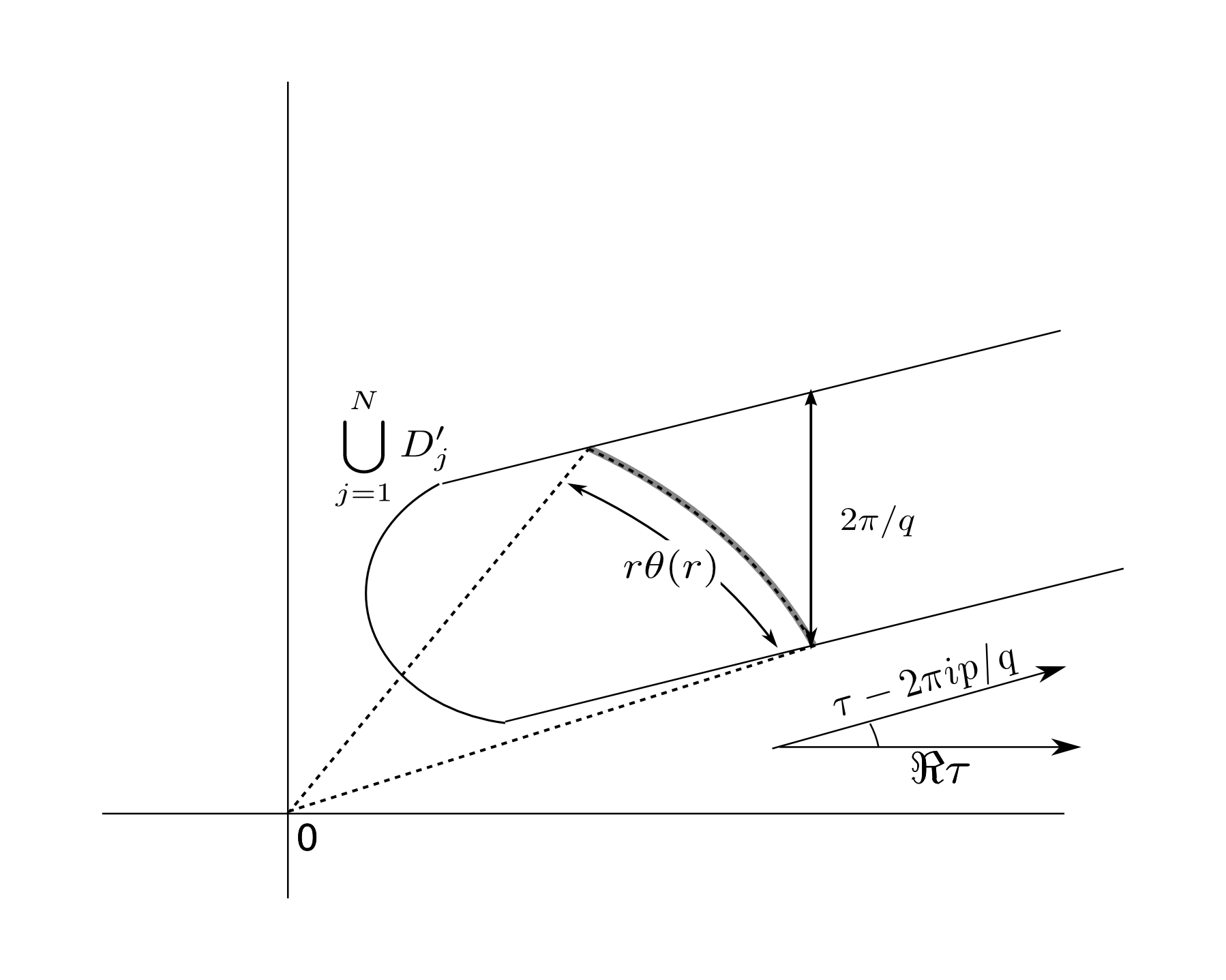
Figure 5.

Therefore from (4.13) it follows that

$$\int\limits_{r_{0}}^{\kappa r}\sum_{j=1}^{N}r\theta_{j}(r)dr \leq\int\limits_{0}^{\frac{\Re\tau}{|\tau-2\pi ip/q|}\kappa r}{\rm len}\bigg{(}\{\Re s=\xi\cap\bigcup_{j=1}^{N}D_{j}^{\prime}\}\bigg{)}d\xi+{\rm const}$$

$$\leq\frac{2\pi}{q}\frac{\Re\tau}{|\tau-2\pi ip/q|}\kappa(r+{\rm const})$$

By substituting the above inequality in (4.16) we get

(4.17) $$\sum_{j=1}^{N}\pi\int\limits_{r_{0}}^{\kappa r}\frac{dr}{r\theta_{j}(r)}\geq\frac{N^{2}q|\tau-2\pi ip/q|}{2\Re\tau}\frac{(\kappa r-r_{0})^{2}}{\kappa(r+{\rm const.})}.$$

Since $|e^{s}|=e^{\Re s}$, the estimate on the left side of (4.15) can be modified as

$$\sum_{j=1}^{N}\log\max_{|s|=r}w_{j}(s) \leq N\log\max_{s\in\bigcup D_{j}^{\prime},|s|=r}v(e^{s})$$

(4.18) $$\leq\max_{s\in\bigcup D_{j}^{\prime},|s|=r}N\Re s\bigg{(}\frac{\log|u^{+}(e^{s})|}{\log|e^{s}|}\bigg{)}.$$

So from (4.15), (4.17) and (4) we get

$$\max_{s\in\bigcup D_{j}^{\prime},|s|=r}N\Re s\bigg{(}\frac{\log|u^{+}(e^{s})|}{\log|e^{s}|}\bigg{)}\geq\frac{N^{2}q|\tau-2\pi ip/q|}{2\Re\tau}\frac{(\kappa r-r_{0})^{2}}{\kappa(r+{\rm const.})}-{\rm const.}$$

and by dividing both sides by $r$, we get

(4.19) $$\max_{s\in\bigcup D_{j}^{\prime},|s|=r}N\frac{\Re s}{|s|}\frac{\log|u^{+}(e^{s})|}{\log|e^{s}|}\geq\frac{N^{2}q|\tau-2\pi ip/q|}{2\Re\tau}\frac{(\kappa r-r_{0})^{2}}{\kappa r(r+{\rm const.})}-\frac{{\rm const.}}{r}.$$

Earlier we have proved that

$$\bigg{|}{\Re s-\frac{\Re\tau}{|\tau-2i\pi p/q|}|s|}\bigg{|}$$

is bounded, i.e.,

$$\lim_{|s|\to\infty}\frac{\Re s}{|s|}=\frac{\Re\tau}{|\tau-2i\pi p/q|}.$$

By taking the limit as $r\to\infty$ in (4.19) we get

(4.20) $$N\frac{\Re\tau}{|\tau-2i\pi p/q|}{\rm ord}u^{+}\geq\frac{\kappa N^{2}q|\tau-2\pi ip/q|}{2\Re\tau}.$$

Since ${\rm ord}u^{+}=\log d/\Re\tau$ and $1/e\leq\kappa<1$ is arbitrary we get

$$\frac{N\log d}{|\tau-2i\pi p/q|}\geq\frac{N^{2}q|\tau-2\pi ip/q|}{2\Re\tau}$$

which reduces to the Yoccoz inequality. ∎

5. Appendix

For a given $\delta>0$ and real numbers $a_{1},a_{2},\ldots,a_{k}$ define a family of subsets $X(i_{2},i_{3},\ldots,i_{k-2})\subset\mathbb{C}^{k}$ where $i_{j}\in\{0,1\}$ for every $j\in\{2,\ldots,k-2\}$ as :

$$X(i_{2},i_{3},\ldots,i_{k-2})=\Big{\{}z\in\mathbb{C}^{k}:\Re\pi_{j-1}(z)\leqslant a_{j-1}-\delta\;\mbox{if}\;i_{j}=0\;\mbox{else}\;\Re\pi_{j-1}(z)\geqslant a_{j-1}+\delta\;\mbox{if}\;i_{j}=1\Big{\}}.$$

Note that $X(i_{2},i_{3},\ldots,i_{k-2})$ is non-empty provided $k>3$.

Theorem 5.1.

Let $\rho(z)=\min\Big{\{}|\pi_{1}(z)|,\ldots,|\pi_{p}(z)|\Big{\}}$. Let $\lambda_{1},\lambda_{2},\ldots,\lambda_{k},a_{1},a_{2},\ldots,a_{k}$ be real constants and let $\delta>0,~{}\eta>0.$ Define a family of maps $\alpha_{j}:\{0,1\}\to\{0,\lambda_{j}\}$ as $\alpha_{j}(0)=0~{},\alpha_{j}(1)=\lambda_{j}$ for all $j=1,2,\ldots,k.$ Then there exists a map $\theta\in Aut_{1}(\mathbb{C}^{k})$ such that

1. $|\theta(z)-z+(\alpha_{1}(1),\alpha_{2}(i_{2}),\ldots,\alpha_{k-2}(i_{k-2}),\alpha_{k-1}(1),\alpha_{k}(1))|<\eta e^{-\rho(z)^{1/4}}$ whenever

   $$z\in X(i_{2},i_{3},\ldots,i_{k-2})\cap\Big{\{}z\in\mathbb{C}^{k}:\Re\pi_{k-2}(z)\geqslant a_{k-2}+\delta,~{}\Re\pi_{k-1}(z)\geqslant a_{k-1}+\delta,~{}\Re\pi_{k}(z)\geqslant a_{k}+\delta\Big{\}}.$$

2. $|\theta(z)-z+(\alpha_{1}(1),\alpha_{2}(i_{2}),\ldots,\alpha_{k-2}(i_{k-2}),\alpha_{k-1}(0),\alpha_{k}(1))|<\eta e^{-\rho(z)^{1/4}}$ whenever

   $$z\in X(i_{2},i_{3},\ldots,i_{k-2})\cap\Big{\{}z\in\mathbb{C}^{k}:\Re\pi_{k-2}(z)\leqslant a_{k-2}-\delta,~{}\Re\pi_{k-1}(z)\geqslant a_{k-1}+\delta,~{}\Re\pi_{k}(z)\geqslant a_{k}+\delta\Big{\}}.$$

3. $|\theta(z)-z+(\alpha_{1}(0),\alpha_{2}(i_{2}),\ldots,\alpha_{k-2}(i_{k-2}),\alpha_{k-1}(1),\alpha_{k}(1))|<\eta e^{-\rho(z)^{1/4}}$ whenever

   $$z\in X(i_{2},i_{3},\ldots,i_{k-2})\cap\Big{\{}z\in\mathbb{C}^{k}:\Re\pi_{k-2}(z)\geqslant a_{k-2}+\delta,~{}\Re\pi_{k-1}(z)\geqslant a_{k-1}+\delta,~{}\Re\pi_{k}(z)\leqslant a_{k}-\delta\Big{\}}.$$

4. $|\theta(z)-z+(\alpha_{1}(0),\alpha_{2}(i_{2}),\ldots,\alpha_{k-2}(i_{k-2}),\alpha_{k-1}(0),\alpha_{p}(1))|<\eta e^{-\rho(z)^{1/4}}$ whenever

   $$z\in X(i_{2},i_{3},\ldots,i_{k-2})\cap\Big{\{}z\in\mathbb{C}^{k}:\Re\pi_{k-2}(z)\leqslant a_{k-2}-\delta,~{}\Re\pi_{k-1}(z)\geqslant a_{k-1}+\delta,~{}\Re\pi_{k}(z)\leqslant a_{k}-\delta\Big{\}}.$$

5. $|\theta(z)-z+(\alpha_{1}(1),\alpha_{2}(i_{2}),\ldots,\alpha_{k-2}(i_{k-2}),\alpha_{k-1}(1),\alpha_{k}(0))|<\eta e^{-\rho(z)^{1/4}}$ whenever

   $$z\in X(i_{2},i_{3},\ldots,i_{k-2})\cap\Big{\{}z\in\mathbb{C}^{k}:\Re\pi_{k-2}(z)\geqslant a_{k-2}+\delta,~{}\Re\pi_{k-1}(z)\leqslant a_{k-1}-\delta,~{}\Re\pi_{k}(z)\geqslant a_{k}-\lambda_{k}+\delta\Big{\}}.$$

6. $|\theta(z)-z+(\alpha_{1}(1),\alpha_{2}(i_{2}),\ldots,\alpha_{k-2}(i_{k-2}),\alpha_{k-1}(0),\alpha_{k}(0))|<\eta e^{-\rho(z)^{1/4}}$ whenever

   $$z\in X(i_{2},i_{3},\ldots,i_{k-2})\cap\Big{\{}z\in\mathbb{C}^{k}:\Re\pi_{k-2}(z)\leqslant a_{k-2}-\delta,~{}\Re\pi_{k-1}(z)\leqslant a_{k-1}-\delta,~{}\Re\pi_{k}(z)\geqslant a_{k}-\lambda_{k}+\delta\Big{\}}.$$

7. $|\theta(z)-z+(\alpha_{1}(0),\alpha_{2}(i_{2}),\ldots,\alpha_{k-2}(i_{k-2}),\alpha_{k-1}(1),\alpha_{k}(0))|<\eta e^{-\rho(z)^{1/4}}$ whenever

   $$z\in X(i_{2},i_{3},\ldots,i_{k-2})\cap\Big{\{}z\in\mathbb{C}^{k}:\Re\pi_{k-2}(z)\geqslant a_{k-2}+\delta,~{}\Re\pi_{k-1}(z)\leqslant a_{k-1}-\delta,~{}\Re\pi_{k}(z)\leqslant a_{k}-\lambda_{k}-\delta\Big{\}}.$$

8. $|\theta(z)-z+(\alpha_{1}(0),\alpha_{2}(i_{2}),\ldots,\alpha_{k-2}(i_{k-2}),\alpha_{k-1}(0),\alpha_{k}(0))|<\eta e^{-\rho(z)^{1/4}}$ whenever

   $$z\in X(i_{2},i_{3},\ldots,i_{k-2})\cap\Big{\{}z\in\mathbb{C}^{k}:\Re\pi_{k-2}(z)\leqslant a_{k-2}-\delta,~{}\Re\pi_{k-1}(z)\leqslant a_{k-1}-\delta,~{}\Re\pi_{k}(z)\leqslant a_{k}-\lambda_{k}-\delta\Big{\}}.$$

Proof.

As in Section 2, we use the Arakelian–Gauthier theorem to establish the existence of entire functions with the following properties:

(i) $$|f_{n}^{1}(z)-\lambda_{1}|\leqslant\frac{1}{n}e^{-|z|^{1/4}}<\eta e^{-|z|^{1/4}}~{}~{}\mbox{if}~{}~{}\Re z\geqslant a_{k}-\lambda_{k}+\delta/2,~{}\mbox{and}$$

$$|f_{n}^{1}(z)-0|\leqslant\frac{1}{n}e^{-|z|^{1/4}}<\eta e^{-|z|^{1/4}}~{}~{}\mbox{if}~{}~{}\Re z\leqslant a_{k}-\lambda_{k}-\delta/2.$$

(ii) $$|f_{n}^{j}(z)-\lambda_{n}|\leqslant\frac{1}{n}e^{-|z|^{1/4}}<\eta e^{-|z|^{1/4}}~{}~{}\mbox{if}~{}~{}\Re z\geqslant a_{j-1}+\delta/2,~{}\mbox{and}$$

$$|f_{n}^{j}(z)-0|\leqslant\frac{1}{n}e^{-|z|^{1/4}}<\eta e^{-|z|^{1/4}}~{}~{}\mbox{if}~{}~{}\Re z\leqslant a_{j-1}-\delta/2,~{}~{}\mbox{where}~{}~{}2\leq j\leq k.$$

Define $\theta_{n}\in{\rm Aut}_{1}(\mathbb{C}^{k})$ as $\theta_{n}(z_{1},z_{2},\ldots,z_{k})=(v_{1},v_{2},\ldots,v_{k})$ as

$$v_{1} =z_{1}+f_{n}^{1}(v_{k}),$$

$$v_{2} =z_{2}+f_{n}^{2}(z_{1}),$$

$$\vdots$$

$$v_{k} =z_{k}+f_{n}^{k}(z_{k-1}).$$

Pick $z\in\mathbb{C}^{k}$ such that $z\in X(i_{2},i_{3},\ldots,i_{k-2})$ for $i_{j}\in\{0,1\}$ for every $1\leq j\leq k-2$ and $\Re\pi_{k-2}(z)\geq a_{j}+\delta,~{}\Re\pi_{k-1}(z)\geq a_{j}+\delta,~{}\Re\pi_{k}(z)\geqslant a_{k}-\lambda_{k}+\delta.$ Then

$$|f_{n}^{j}(z_{j-1})-\alpha_{j}(i_{j})|=|\pi_{j}(\theta_{n}(z))-\pi_{j}(z)+\alpha_{j}(i_{j})|<\eta e^{-\rho(z)^{1/4}}$$

for $2\leq j\leq k-2$ and

$$|f_{n}^{j}(z_{j-1})-\lambda_{j}|=|\pi_{j}(\theta_{n}(z))-\pi_{j}(z)+\lambda_{j}|<\eta e^{-\rho(z)^{1/4}}$$

for $j=k-1,k.$ Therefore

$$\Re v_{k}\geqslant\Re z_{k}-\lambda_{k}-\eta\geqslant a_{k}-\lambda_{k}+\delta/2$$

and hence

$$|\pi_{1}(\theta_{n}(z))-\pi_{1}(z)+\lambda_{1}|=|f_{n}^{1}(v_{k})-\lambda_{1}|<e^{-|v_{k}|^{1/4}}/n.$$

Since $|v_{k}|>|z_{k}|-|\lambda_{k}|-1$ and $t^{1/4}-(t-\lambda_{3}-1)^{1/4}\to 0$ as $t\to\infty$ there exists a constant $C>0$ such that

$$e^{-|v_{k}|^{1/4}}<Ce^{-|z_{k}|^{1/4}}.$$

If we choose $n$ large enough so that $C/n<\eta$ and $1/n<\eta$, then $\theta_{n}$ satisfies condition (i) of the theorem. Similarly it can be shown that for large $n$, $\theta_{n}$ satisfies all the other conditions. ∎

In analogy with Theorem 2.2 which has $2^{3}=8$ regions where the map $\theta$ has apriori prescribed behaviour, one would imagine that there should be $2^{k}$ regions in Theorem 5.1 with specified behaviour for the map obtained there. However, the behaviour of that map can be summarised within the conditions (i) - (viii) because of its shift-like nature. The set $X(i_{2},i_{3},\ldots,i_{k-2})$ is the region where the shift–like behaviour is similar for the coordinates $z_{j}$ with $1\leq j\leq k-3$.

References

- [1] N. U. Arakelian and P. Gauthier: On tangential approximation by entire functions, Izv. Akad. Nauk Armyan. SSSR (6) 17 (1982), 421-441; English transi, in Soviet J. Contemporary Math. 17(1982), 1–22. See [7] in [6].
- [2] E. Bedford and V. Pambuccian: Dynamics of shift-like polynomial diffeomorphisms of , Conform. Geom. Dyn. 2 (1998), 45–55 (electronic).
- [3] E. Bedford and J. Smillie: Polynomial diffeomorphisms of . VI. Connectivity of J, Ann. of Math. (2) 148 (1998), no. 2, 695–735.
- [4] Gregory T. Buzzard: Tame sets, dominating maps, and complex tori, Trans. Amer. Math. Soc. 355 (2003), no. 6, 2557–2568 (electronic).
- [5] S. Cantat: Croissance des variétés instables, Ergodic Theory Dynam. Systems 23 (2003), no. 4, 1025–1042.
- [6] P. G. Dixon, J. Esterle: Michael’s problem and the Poincaré–Fatou–Bieberbach phenomenon, Bull. Amer. Math. Soc. (N.S.) 15 (1986), no. 2, 127–187.
- [7] J. E. Fornaess, N. Sibony: Complex Hénon mappings in and Fatou-Bieberbach domains, Duke Math. J. 65 (1992), no. 2, 345–380.
- [8] J. Globevnik: On Fatou–Bieberbach domains, Math. Z. 229 (1998), no. 1, 91–106.
- [9] J. Globevnik, B. Stensones: Holomorphic embeddings of planar domains into , Math. Ann. 303 (1995), no. 4, 579–597.
- [10] V. Guedj, N. Sibony: Dynamics of polynomial automorphisms of , Ark. Mat. 40 (2002), no. 2, 207–243.
- [11] W. K. Hayman: Subharmonic Functions, Vol. 2, Academic Press Inc., 1989.
- [12] J. Hubbard: Local connectivity of Julia sets and bifurcation loci: three theorems of J. C. Yoccoz, Topological methods in modern mathematics (Stony Brook, NY, 1991), 467–511, Publish or Perish, Houston, TX, 1993.
- [13] T. Jin: Unstable manifolds and the Yoccoz inequality for complex Hénon mappings, Indiana Univ. Math. J. 52 (2003), no. 3, 727–751.
- [14] S. Morosawa, Y. Nishimura, M. Taniguchi, T. Ueda: Holomorphic dynamics, Cambridge University Press, 2000.
- [15] J. P. Rosay, W. Rudin: Holomorphic maps from to , Trans. Amer. Math. Soc. 310 (1988), no. 1, 47–86.
- [16] J. P. Rosay, W. Rudin: Growth of volume in Fatou-Bieberbach regions, Publ. Res. Inst. Math. Sci. 29 (1993), no. 1, 161–166.
- [17] N. Sibony: Dynamique des applications rationnelles de , Dynamique et géométrie complexes (Lyon, 1997), ix–x, xi–xii, 97–185, Panor. Synthéses, 8, Soc. Math. France, Paris, 1999.
- [18] B. Stensones: Fatou-Bieberbach domains with –smooth boundary, Ann. of Math. (2) 145 (1997), no. 2, 365–377.
- [19] S.Sternberg: Local contractions and a theorem of Poincaré, Amer. J. Math 79(1957) 809–823.
- [20] E. F. Wold: Fatou–Bieberbach domains, Internat. J. Math. 16 (2005), no. 10, 1119–1130.