Pion photo- and electroproduction with chiral MAID

Abstract

We present a calculation of pion photo- and electroproduction in manifestly Lorentz-invariant baryon chiral perturbation theory up to and including order $q^{4}$. We fix the low-energy constants by fitting experimental data in all available reaction channels. Our results can be accessed via a web interface, the so-called chiral MAID. We explain how our program works and how it can be used for further analysis.

I Introduction

The pion triplet ($\pi^{+},\pi^{0},\pi^{-}$) comprises the lightest hadrons which are of fundamental importance in our understanding of the strong interactions. In 1935, Yukawa introduced a field mediating the interaction between the proton and the neutron to explain the nature of the forces in the nucleus Yukawa:1935xg . Based on experimental results for the mass defect of deuterium, he estimated the mass associated with the quantum field of the exchanged particle to be $200$ times as large as the electron mass. From the present-day perspective, one-pion exchange is responsible for the long-range part of the nucleon-nucleon interaction (see, e.g., Refs. Epelbaum:2008ga ; Machleidt:2011zz for a review). In 1947, charged pions, produced by cosmic rays at high altitudes, were discovered by Lattes et al. Lattes:1947mw in terms of their decay into muons and neutrinos. Subsequently, charged pions were produced in the laboratory by impinging alpha particles on a carbon target Gardner:1948 ; Burfening:1987na . On the other hand, neutral pions were first produced in terms of proton-nucleon collisions in nuclei Bjorklund:1950zz and photoproduction on nuclei Panofsky:1950gj .

Ever since the nineteen-fifties, the electromagnetic production of pions on the nucleon has been an important source of information on the pion-nucleon interaction. On the theoretical side, the low-energy theorem (LET) of Kroll and Ruderman Kroll:1953vq provided a prediction for the matrix element for charged pion photoproduction at threshold. Based on a few assumptions such as covariance, gauge invariance, and renormalizability, the theorem states that the photoproduction of charged pions at threshold computed to lowest order in the pion-nucleon mass ratio, $\mu=M_{\pi}/m_{N}$, but to arbitrary order in the pion-nucleon coupling constant is equivalent to a calculation in second-order perturbation theory with pseudoscalar coupling, provided that the pion-nucleon coupling constant and the nucleon mass are replaced by their renormalized values. It was also shown that the $\pi^{0}$ production amplitude vanishes in the limit $\mu\to 0$. Multipole expansions for photo- and electroproduction were derived in Refs. Chew:1957tf and Dennery:1961zz , respectively. Because of the large value of the pion-nucleon coupling constant, perturbative methods turned out to be of limited use and, thus, the treatment of pion production focussed on dispersive techniques (see Refs. Hanstein:1996bd ; Hanstein:1997tp ; Kamalov:2002wk ; Pasquini:2004nq ; Pasquini:2006yi ; Pasquini:2007fw ; Drechsel:2007gz for more recent applications).

A new twist originated from the interpretation of pions as the (almost) massless Goldstone bosons of a spontaneous breakdown of chiral symmetry Nambu:1960xd ; Nambu:1961tp ; Goldstone:1961eq ; Goldstone:1962es . As was first discussed in Ref. Nambu:1997wa , chirality conservation in the strong interactions results in the bremsstrahlung of soft pions in any reaction with a change of nucleon helicity. The consequences of this observation for the case of pion electroproduction were first worked out by Nambu and Shrauner Nambu:1997wb . In particular, as a generalization of the Kroll-Ruderman theorem for a virtual photon, their result for the production of charged pions involved the normalized isovector axial form factor.

In quantum chromodynamics (QCD), chiral symmetry originates from the zero-mass limit of $u$ and $d$ quarks in the two-flavor case, with a straightforward generalization if the strange-quark mass is also taken to zero. Although in the pre-QCD era the dynamical origin of chiral symmetry was not known, the symmetry structure was inferred from electromagnetic and weak hadron currents and summarized in terms of the so-called current algebra, i.e., equal-time commutation relations involving vector- and axial-vector currents (see, e.g., Refs. Adler:1968 ; Treiman:1972 ; Alfaro:1973 ). In particular, as first pointed out by Gell-Mann, the equal-time commutation relations still play an important role even if the symmetry is explicitly broken GellMann:1962xb . The so-called partially conserved axial-vector current (PCAC) hypothesis Nambu:1960xd ; Bernstein:1960a ; GellMann:1960np ; Bernstein:1960b assumed that the divergence of the axial-vector current is proportional to a renormalized pion field and would disappear in the limit of massless pions. Numerous predictions have been derived from current algebra (see Refs. Adler:1968 ; Treiman:1972 ; Alfaro:1973 for an overview). For example, as an application to pion photoproduction, Fubini, Furlan, and Rossetti derived dispersion relations, connecting the isoscalar and isovector anomalous magnetic moments of the nucleon with the forward production amplitude for soft pions Fubini:1965 ; Pasquini:2004nq ; Bernard:2005dj . Another example is given by the Adler-Gilman relation Adler:1966gd , providing a consistency relation for pion electroproduction in terms of a chiral Ward identity Adler:1966gd ; Fuchs:2003vw . Finally, by including the PCAC hypothesis, corrections for the threshold amplitudes beyond the LET of Kroll and Ruderman were investigated in, e.g., Refs. DeBaenst:1971hp ; Vainshtein:1972ih ; Scherer:1991cy . A comprehensive overview of the various phenomenological implications of PCAC and current algebra for pion electroproduction can be found in Ref. Amaldi:1979vh .

As an alternative method to the often unwieldy soft-pion techniques, Weinberg constructed an effective Lagrangian for soft-pion interactions reproducing the results of current algebra Weinberg:1966fm . While in the beginning phenomenological Lagrangians were applied with the understanding that they should only be used at tree level Weinberg:1966fm ; Schwinger:1967tc ; Weinberg:1968de ; Coleman:1969sm ; Callan:1969sn , in 1979 it was pointed out by Weinberg Weinberg:1978kz that corrections to the chiral limit could be calculated systematically in terms of an effective field theory (EFT) program. The approach is based on a perturbative calculation using a momentum expansion based on the most general Lagrangian consistent with chiral symmetry. With QCD as the underlying fundamental theory, the corresponding low-energy EFT in terms of pions and nucleons as effective degrees of freedom is chiral perturbation theory (ChPT) Weinberg:1978kz ; Gasser:1983yg ; Gasser:1987rb (see, e.g., Refs. Ecker:1994gg ; Bernard:1995dp ; Scherer:2002tk ; Scherer:2012zzd for an introduction). Assigning a suitable order to the explicit symmetry breaking due to the quark masses, it is possible to include quark-mass effects perturbatively.

Until the 1980s, there was little doubt concerning the validity of the low-energy predictions for pion photoproduction. In particular, the results for the charged channels, which are dominated by the Kroll-Ruderman theorem, were in good agreement with the available data Adamovich:1976 . However, renewed interest in neutral pion photoproduction at threshold was triggered by experimental data Mazzucato:1986dz ; Beck:1990da which indicated a serious disagreement with the predictions for the $s$-wave electric dipole amplitude $E_{0+}$ based on current algebra and PCAC DeBaenst:1971hp . This discrepancy was explained with the aid of ChPT Bernard:1991rt . Pion loops, which are beyond the current-algebra framework, generate infrared singularities in the scattering amplitude which then modify the predicted low-energy expansion of $E_{0+}$ (see also Ref. Davidson:1993et ). Subsequently, several experiments investigated pion photo- and electroproduction in the threshold region Welch:1992ex ; Wang:1992 ; Liu:1994 ; vandenBrink:1995uka ; Blomqvist:1996tx ; Fuchs:1996ja ; Bergstrom:1996fq ; Bernstein:1996vf ; Bergstrom:1997jc ; Kovash:1997tj ; Bergstrom:1998ec ; Distler:1998ae ; Liesenfeld:1999mv ; Korkmaz:1999sg ; Schmidt:2001vg ; Merkel:2001qg ; baumann ; Weis:2007kf ; Merkel:2009zz ; Merkel:2011cf ; Hornidge:2012ca ; Hornidge:2013qka ; Lindgren:2013eta . From the theoretical side, all of the different reaction channels of pion photo- and electroproduction near threshold were extensively investigated by Bernard et al. within the framework of heavy-baryon chiral perturbation theory (HBChPT) Bernard:1992qa ; Bernard:1992nc ; Bernard:1992ys ; Bernard:1993bq ; Bernard:1994dt ; Bernard:1994gm ; Bernard:1995cj ; Bernard:1996ti ; Bernard:1996bi ; Fearing:2000uy ; Bernard:2001gz . In the beginning, the manifestly Lorentz-invariant or relativistic formulation of ChPT (RChPT) was abandoned, as it seemingly had a problem with respect to power counting when loops containing internal nucleon lines come into play. Therefore, HBChPT became a standard tool for the analysis of pion photo- and electroproduction in the threshold region (see, e.g., Ref. FernandezRamirez:2012nw ). In the meantime, the development of the infrared regularization (IR) scheme Becher:1999he and the extended on-mass-shell (EOMS) scheme Gegelia:1999gf ; Fuchs:2003qc offered a solution to the power-counting problem, and RChPT became popular again. For example, pion-nucleon scattering was analyzed at $O(q^{4})$ in both IR and EOMS schemes in Refs. Becher:2001hv and Chen:2012nx , respectively, and at $O(q^{3})$ in the EOMS scheme including the $\Delta$ resonance Alarcon:2012kn .

The aim of the present article is twofold. First, by presenting a full $O(q^{4})$ calculation of pion photo- and electroproduction in the framework of RChPT, we extend the results of Ref. Hilt:2013uf for neutral pion photoproduction on the proton. Second, we present the so-called chiral MAID ($\chi$MAID) website . This program, accessible via a web interface, provides the numerical results of these calculations.

II Pion photo- and electroproduction

In this section we provide a short introduction to our notation for describing the electroproduction of pions,

$$e(k_{i})+N(p_{i})\rightarrow e(k_{f})+N(p_{f})+\pi(q).$$ (1)

The interaction of the electron with the nucleon is of purely electromagnetic type and, due to the small coupling $\alpha=e^{2}/(4\pi)\approx 1/137$, the process can be described in the so-called one-photon-exchange approximation (see Fig. 1). In this approximation, the invariant amplitude ${\cal M}$ may be interpreted as the inner product of the polarization vector $\epsilon_{\mu}$ of the virtual photon (four-momentum $k=k_{i}-k_{f}$) and the hadronic transition current matrix element ${\cal M}^{\mu}$,

$${\cal M}=\epsilon_{\mu}{\cal M}^{\mu},$$ (2)

where

$$\epsilon_{\mu}=e\frac{\bar{u}(k_{f})\gamma_{\mu}u(k_{i})}{k^{2}}$$ (3)

and

$${\cal M}^{\mu}=-ie\langle N(p_{f}),\pi(q)|J^{\mu}(0)|N(p_{i})\rangle.$$ (4)

Therefore, it is sufficient to consider the process

$$\gamma^{*}(k)+N(p_{i})\rightarrow N(p_{f})+\pi(q),$$ (5)

where $\gamma^{\ast}$ refers to a virtual photon.

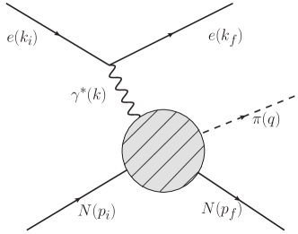
Figure 1: Pion electroproduction in the one-photon-exchange approximation. The momenta of the incoming and outgoing nucleons are $p_{i}$ and $p_{f}$, respectively. The momentum of the incoming/outgoing electron is $k_{i}$/$k_{f}$, where $k=k_{i}-k_{f}$ represents the momentum of the single exchanged virtual photon. The momentum of the pion is labeled $q$. In the case of pion photoproduction, the leptonic vertex and the photon propagator are replaced by the polarization vector of the real photon. The shaded circle represents the full hadronic vertex.

The invariant amplitude of pion photoproduction is obtained by replacing the polarization vector of the virtual photon by the polarization vector of a real photon and taking $k^{2}=0$. Treating the virtual photon as a particle of “mass” $k^{2}=-Q^{2}$, the Mandelstam variables $s$, $t$, and $u$ are defined as

$$s=(p_{i}+k)^{2}=(p_{f}+q)^{2},\ u=(p_{i}-q)^{2}=(p_{f}-k)^{2},\ t=(p_{i}-p_{f})^{2}=(q-k)^{2},$$ (6)

and fulfill

$$s+t+u=2m_{N}^{2}+M_{\pi}^{2}-Q^{2},$$ (7)

where $m_{N}$ and $M_{\pi}$ denote the nucleon mass and the pion mass, respectively. In the case of photoproduction ($k^{2}=0$) only two of the Mandelstam variables are independent. In the center-of-mass (cm) frame, the energies of the photon, $k_{0}$, and the pion, $E_{\pi}$, are given by

$$k_{0}=\frac{W^{2}-m_{N}^{2}-Q^{2}}{2W},\ E_{\pi}=\frac{W^{2}+M_{\pi}^{2}-m_{N}^{2}}{2W},$$ (8)

where $W=\sqrt{s}$ is the cm total energy. The equivalent real photon laboratory energy $E_{\gamma}^{\textnormal{lab}}$ is given by

$$E_{\gamma}^{\textnormal{lab}}=\frac{W^{2}-m_{N}^{2}}{2m_{N}}.$$ (9)

The cm scattering angle $\Theta_{\pi}$ between the pion three-momentum and the $z$-axis, defined by the incoming (virtual) photon, can be related to the Mandelstam variable $t$ via

$$t=M_{\pi}^{2}-2(E_{\gamma}E_{\pi}-|\vec{k}||\vec{q}\hskip 1.42271pt|\cos\Theta_{\pi}).$$ (10)

The matrix element of pion electroproduction can be parametrized in terms of the so-called Ball amplitudes Ball:1961zza , which are defined in a Lorentz-covariant way and are convenient for calculating the process $\gamma^{*}(k)+N(p_{i})\rightarrow N(p_{f})+\pi(q)$,

$$-ie\langle{N^{\prime}\pi}|J^{\mu}(0)|{N}\rangle=\bar{u}(p_{f})\left(\sum_{i=1}^{8}B_{i}V_{i}^{\mu}\right)u(p_{i}).$$ (11)

In Eq. (11), $J^{\mu}$ is the electromagnetic current operator in units of the elementary charge $e>0$, and $u(p_{i})$ and $\bar{u}(p_{f})$ are the Dirac spinors of the nucleon in the initial and final states, respectively. In the following, our convention differs slightly from Ball’s original definition. We use

$$\begin{split}V_{1}^{\mu}&=\gamma^{\mu}\gamma_{5},\quad V_{2}^{\mu}=\gamma_{5}P^{\mu},\quad V_{3}^{\mu}=\gamma_{5}q^{\mu},\quad V_{4}^{\mu}=\gamma_{5}k^{\mu},\\ V_{5}^{\mu}&=\gamma^{\mu}\not{k}\gamma_{5},\quad V_{6}^{\mu}=\not{k}\gamma_{5}P^{\mu},\quad V_{7}^{\mu}=\not{k}\gamma_{5}q^{\mu},\quad V_{8}^{\mu}=\not{k}\gamma_{5}k^{\mu},\end{split}$$ (12)

with $P=(p_{i}+p_{f})/2$ and $\not{k}=\gamma^{\mu}k_{\mu}$. Electromagnetic current conservation, $k_{\mu}{\cal M}^{\mu}=0$, leads to the following two constraints for the amplitudes $B_{i}$,

$$\begin{split}B_{1}+B_{6}k\cdot P+B_{7}k\cdot q+B_{8}k^{2}&=0,\\ B_{2}k\cdot P+B_{3}k\cdot q+B_{4}k^{2}+B_{5}k^{2}&=0.\end{split}$$ (13)

Thus, only six independent amplitudes are required for the description of pion electroproduction. Furthermore, in pion photoproduction ($k^{2}=0$) only four independent amplitudes survive.

Besides Eq. (11), several other parameterizations exist for the matrix element of Eq. (4). Here, we focus on those we used for our calculations. The parameterization of Ref. Drechsel:1992pn takes care of current conservation already from the beginning and, thus, contains only six independent amplitudes $A_{i}$,

$$\mathcal{M}^{\mu}=\bar{u}(p_{f})\left(\sum_{i=1}^{6}A_{i}M_{i}^{\mu}\right)u(p_{i}),$$ (14)

with

$$\begin{split}M_{1}^{\mu}&=-\frac{i}{2}\gamma_{5}\left(\gamma^{\mu}\not{k}-\not{k}\gamma^{\mu}\right),\\ M_{2}^{\mu}&=2i\gamma_{5}\left[P^{\mu}k\cdot\left(q-\frac{1}{2}k\right)-\left(q^{\mu}-\frac{1}{2}k^{\mu}\right)k\cdot P\right],\\ M_{3}^{\mu}&=-i\gamma_{5}\left(\gamma^{\mu}k\cdot q-\not{k}q^{\mu}\right),\\ M_{4}^{\mu}&=-2i\gamma_{5}\left(\gamma^{\mu}k\cdot P-\not{k}P^{\mu}\right)-2m_{N}M_{1}^{\mu},\\ M_{5}^{\mu}&=i\gamma_{5}\left(k^{\mu}k\cdot q-q^{\mu}k^{2}\right),\\ M_{6}^{\mu}&=-i\gamma_{5}\left(\not{k}k^{\mu}-\gamma^{\mu}k^{2}\right).\end{split}$$ (15)

Note that each structure $M_{i}^{\mu}$ satisfies $k_{\mu}M^{\mu}_{i}=0$.

The so-called Chew-Goldberger-Low-Nambu (CGLN) amplitudes $\mathcal{F}_{i}$ are another common parameterization Chew:1957tf ; Dennery:1961zz . These amplitudes are defined in the cm frame via

$$\epsilon_{\mu}\bar{u}(p_{f})\left(\sum_{i=1}^{6}A_{i}M_{i}^{\mu}\right)u(p_{i})=\frac{4\pi W}{m_{N}}\chi_{f}^{\dagger}\mathcal{F}\chi_{i},$$ (16)

where $\chi_{i}$ and $\chi_{f}$ denote initial and final Pauli spinors. Electromagnetic current conservation allows one to work in a gauge where the polarization vector of the virtual photon has a vanishing time component. In terms of the polarization vector of Eq. (3) this is achieved by introducing the vector Amaldi:1979vh

$$a^{\mu}=\epsilon^{\mu}-k^{\mu}\frac{\epsilon_{0}}{k_{0}}=\epsilon^{\mu}-k^{\mu}\frac{\vec{k}\cdot\vec{\epsilon}}{k_{0}^{2}},$$ (17)

where use of $k_{\mu}\epsilon^{\mu}=0$ has been made. Splitting $\vec{a}$ into a longitudinal and a transversal piece,

$$\begin{split}\vec{a}&=\vec{a}_{\parallel}+\vec{a}_{\perp},\\ \vec{a}_{\parallel}&=\vec{a}\cdot\hat{k}\,\hat{k}=\frac{k^{2}}{k_{0}^{2}}\vec{\epsilon}\cdot\hat{k}\,\hat{k},\\ \vec{a}_{\perp}&=\vec{a}-\vec{a}_{\parallel}=\vec{\epsilon}-\vec{\epsilon}\cdot\hat{k}\,\hat{k}=\vec{\epsilon}_{\perp},\end{split}$$ (18)

$\mathcal{F}$ may be written as

$$\begin{split}\mathcal{F}=&i\vec{\sigma}\cdot\vec{a}_{\perp}\mathcal{F}_{1}+\vec{\sigma}\cdot\hat{q}\,\vec{\sigma}\cdot\hat{k}\times\vec{a}_{\perp}\mathcal{F}_{2}+i\vec{\sigma}\cdot\hat{k}\,\hat{q}\cdot\vec{a}_{\perp}\mathcal{F}_{3}+i\vec{\sigma}\cdot\hat{q}\,\hat{q}\cdot\vec{a}_{\perp}\mathcal{F}_{4}\\ &+i\vec{\sigma}\cdot\hat{k}\,\hat{k}\cdot\vec{a}_{\parallel}\mathcal{F}_{5}+i\vec{\sigma}\cdot\hat{q}\,\hat{k}\cdot\vec{a}_{\parallel}\mathcal{F}_{6},\end{split}$$ (19)

where $\hat{q}$ and $\hat{k}$ denote unit vectors in the direction of the pion and the photon, respectively. For the case of pion photoproduction, only the first four terms of Eq. (19) contribute.

The connection between the Ball amplitudes, invariant amplitudes, and CGLN amplitudes can be found in Appendix A. The CGLN amplitudes can be expanded in a multipole series Chew:1957tf ; Dennery:1961zz ; Amaldi:1979vh ,

$$\begin{split}\mathcal{F}_{1}&=\sum_{l=0}^{\infty}\Big{\{}\big{[}lM_{l+}+E_{l+}\big{]}P^{\prime}_{l+1}(x)+\big{[}(l+1)M_{l-}+E_{l-}\big{]}P^{\prime}_{l-1}(x)\Big{\}},\\ \mathcal{F}_{2}&=\sum_{l=1}^{\infty}\Big{\{}(l+1)M_{l+}+lM_{l-}\Big{\}}P^{\prime}_{l}(x),\\ \mathcal{F}_{3}&=\sum_{l=1}^{\infty}\Big{\{}\big{[}E_{l+}-M_{l+}\big{]}P^{\prime\prime}_{l+1}(x)+\big{[}E_{l-}+M_{l-}\big{]}P^{\prime\prime}_{l-1}(x)\Big{\}},\\ \mathcal{F}_{4}&=\sum_{l=2}^{\infty}\Big{\{}M_{l+}-E_{l+}-M_{l-}-E_{l-}\Big{\}}P^{\prime\prime}_{l}(x),\\ \mathcal{F}_{5}&=\sum_{l=0}^{\infty}\Big{\{}(l+1)L_{l+}P^{\prime}_{l+1}-lL_{l-}P^{\prime}_{l}(x)\Big{\}},\\ \mathcal{F}_{6}&=\sum_{l=1}^{\infty}\Big{\{}lL_{l-}-(l+1)L_{l+}\Big{\}}P^{\prime}_{l}(x),\end{split}$$ (20)

where $x=\cos\Theta_{\pi}=\hat{q}\cdot\hat{k}$. In Eq. (20), $P_{l}(x)$ is a Legendre polynomial of degree $l$, $P^{\prime}_{l}=dP_{l}/dx$ and so on, with $l$ denoting the orbital angular momentum of the pion-nucleon system in the final state. The multipoles $E_{l\pm}$, $M_{l\pm}$, and $L_{l\pm}$ are functions of the cm total energy $W$ and the photon virtuality $Q^{2}$ and refer to transversal electric and magnetic transitions and longitudinal transitions, respectively. The subscript $l\pm$ denotes the total angular momentum $j=l\pm 1/2$ in the final state. By inverting the above equations, the angular dependence can be completely projected out Adler:1968tw ; Davidson:1995jm ,

$$\begin{split}E_{l+}=&\int_{-1}^{1}\frac{dx}{2(l+1)}\Big{[}P_{l}\mathcal{F}_{1}-P_{l+1}\mathcal{F}_{2}\\ &+\frac{l}{2l+1}(P_{l-1}-P_{l+1})\mathcal{F}_{3}+\frac{l+1}{2l+3}(P_{l}-P_{l+2})\mathcal{F}_{4}\Big{]},\\ E_{l-}=&\int_{-1}^{1}\frac{dx}{2l}\Big{[}P_{l}\mathcal{F}_{1}-P_{l-1}\mathcal{F}_{2}\\ &-\frac{l+1}{2l+1}(P_{l-1}-P_{l+1})\mathcal{F}_{3}+\frac{l}{2l-1}(P_{l}-P_{l-2})\mathcal{F}_{4}\Big{]},\\ M_{l+}=&\int_{-1}^{1}\frac{dx}{2(l+1)}\left[P_{l}\mathcal{F}_{1}-P_{l+1}\mathcal{F}_{2}-\frac{1}{2l+1}(P_{l-1}-P_{l+1})\mathcal{F}_{3}\right],\\ M_{l-}=&\int_{-1}^{1}\frac{dx}{2l}\left[-P_{l}\mathcal{F}_{1}+P_{l-1}\mathcal{F}_{2}+\frac{1}{2l+1}(P_{l-1}-P_{l+1})\mathcal{F}_{3}\right],\\ L_{l+}=&\int_{-1}^{1}\frac{dx}{2(l+1)}\left[P_{l+1}\mathcal{F}_{6}+P_{l}\mathcal{F}_{5}\right],\\ L_{l-}=&\int_{-1}^{1}\frac{dx}{2l}\left[P_{l-1}\mathcal{F}_{6}+P_{l}\mathcal{F}_{5}\right].\end{split}$$ (21)

In the threshold region, the multipoles $\mathcal{M}_{l\pm}$ ($\mathcal{M}=E,M,L$) are proportional to $|\vec{q}|^{l}$. To get rid of this purely kinematical dependence, one introduces reduced multipoles $\overline{\mathcal{M}}_{l\pm}$ via

$$\overline{\mathcal{M}}_{l\pm}=\frac{\mathcal{M}_{l\pm}}{|\vec{q}|^{l}}.$$ (22)

Due to the assumed isospin symmetry, the process involves only three independent isospin structures for the four physical channels Chew:1957tf . Any amplitude $M$ for producing a pion with Cartesian isospin index $a$ can be decomposed as

$$M(\pi^{a})=\chi_{f}^{\dagger}\left(i\epsilon^{a3b}\tau^{b}M^{(-)}+\tau^{a}M^{(0)}+\delta^{a3}M^{(+)}\right)\chi_{i},\qquad a=1,2,3,$$ (23)

where $\chi_{i}$ and $\chi_{f}$ denote the isospinors of the initial and final nucleons, respectively, and $\tau^{a}$ are the Pauli matrices. The isospin amplitudes corresponding to $A_{i}$ of Eq. (14) obey a crossing symmetry,

$$\begin{split}A^{(0,+)}_{i}&\stackrel{{\scriptstyle s\leftrightarrow u}}{{\longrightarrow}}\eta_{i}A^{(0,+)}_{i},\\ A^{(-)}_{i}&\stackrel{{\scriptstyle s\leftrightarrow u}}{{\longrightarrow}}-\eta_{i}A^{(-)}_{i},\end{split}$$ (24)

where $\eta_{i}=1$ for $i=1,2,4$ and $\eta_{i}=-1$ for $i=3,5,6$. The physical reaction channels are related to the isospin channels via

$$\begin{split}A_{i}(\gamma^{(*)}p\rightarrow n\pi^{+})&=\sqrt{2}\left(A_{i}^{(-)}+A_{i}^{(0)}\right),\\ A_{i}(\gamma^{(*)}p\rightarrow p\pi^{0})&=A_{i}^{(+)}+A_{i}^{(0)},\\ A_{i}(\gamma^{(*)}n\rightarrow p\pi^{-})&=-\sqrt{2}\left(A_{i}^{(-)}-A_{i}^{(0)}\right),\\ A_{i}(\gamma^{(*)}n\rightarrow n\pi^{0})&=A_{i}^{(+)}-A_{i}^{(0)}.\end{split}$$ (25)

In the one-photon-exchange approximation, the differential cross section can be written as

$$\frac{d\sigma}{d\mathcal{E}_{f}d\Omega_{f}d\Omega_{\pi}^{\textnormal{\,cm}}}=\Gamma\frac{d\sigma_{v}}{d\Omega_{\pi}^{\textnormal{\,cm}}},$$ (26)

where the flux of the virtual photon is given by

$$\Gamma=\frac{\alpha}{2\pi^{2}}\frac{\mathcal{E}_{f}}{\mathcal{E}_{i}}\frac{k_{\gamma}}{Q^{2}}\frac{1}{1-\epsilon}.$$ (27)

In Eq. (27), $\mathcal{E}_{i}$ and $\mathcal{E}_{f}$ denote the energy of the initial and final electrons in the laboratory frame, respectively, and $k_{\gamma}=(W^{2}-m_{N}^{2})/(2m_{N})$ is the so-called photon equivalent energy in the laboratory frame. The parameter $\epsilon$ expresses the transverse polarization of the virtual photon in the laboratory frame. In terms of laboratory electron variables it is given by

$$\epsilon=\left(1+2\frac{\vec{k}^{2}}{Q^{2}}\tan^{2}{\left(\frac{\Theta_{e}}{2}\right)}\right)^{-1},$$ (28)

where $\Theta_{e}$ is the scattering angle of the electron.

For an unpolarized target and without recoil polarization detection, the virtual-photon differential cross section for pion production (subscript $v$) can be further decomposed as Drechsel:1992pn

$$\frac{d\sigma_{v}}{d\Omega_{\pi}}=\frac{d\sigma_{T}}{d\Omega_{\pi}}+\epsilon\frac{d\sigma_{L}}{d\Omega_{\pi}}+\sqrt{2\epsilon(1+\epsilon)}\frac{d\sigma_{LT}}{d\Omega_{\pi}}\cos\Phi_{\pi}+\epsilon\frac{d\sigma_{TT}}{d\Omega_{\pi}}\cos{2\Phi_{\pi}}+h\sqrt{2\epsilon(1-\epsilon)}\frac{d\sigma_{LT^{\prime}}}{d\Omega_{\pi}}\sin{\Phi_{\pi}},$$ (29)

where it is understood that the variables of the individual virtual-photon cross sections $d\sigma_{T}/d\Omega_{\pi}$ etc. refer to the cm frame. For further details, especially concerning polarization observables, we refer to Ref. Drechsel:1992pn . The connection to the CGLN amplitudes can be found in Appendix A. Now we have all necessary formulas at hand to calculate pion electroproduction in an arbitrary covariant and gauge-invariant framework. In the following section, we will introduce ChPT as an effective field theory which will allow us to calculate pion production. The upper limit for the cm total energy $W$ is restricted by the fact that we consider pion and nucleon degrees of freedom, only, and do not include the $\Delta(1232)$ resonance Hemmert:1997ye ; Hacker:2005fh ; Pascalutsa:2005vq . Furthermore, given the experience of the description of electromagnetic form factors, a conservative/optimistic estimate for the upper limit of momentum transfers is $Q^{2}=0.1/0.2$ GeV². The inclusion of vector and axial-vector mesons leads to a much improved description of the electromagnetic and axial form factors, respectively Kubis:2000zd ; Schindler:2005ke ; Schindler:2006it ; Bauer:2012pv .

III Chiral perturbation theory

So far, an ab initio QCD calculation of electromagnetic pion production in the low-energy regime is not yet available. However, essential constraints of QCD, resulting from chiral symmetry, its spontaneous breakdown, and the explicit breaking due to the quark masses, may be analyzed in terms of an effective field theory, namely, chiral perturbation theory (see, e.g., Refs. Ecker:1994gg ; Bernard:1995dp ; Scherer:2002tk ; Scherer:2012zzd for an introduction). Starting point is a global $\mbox{SU}(2)_{L}\times\mbox{SU}(2)_{R}\times\mbox{U}(1)_{V}$ symmetry (chiral symmetry) of QCD for massless $u$ und $d$ quarks, which is spontaneously broken down to $\mbox{SU}(2)_{V}\times\mbox{U}(1)_{V}$ in the QCD ground state. In ChPT, the dynamics is expressed in terms of effective degrees of freedom (initially only pions, subsequently also nucleons, etc.) instead of the fundamental degrees of freedom of QCD (quarks and gluons). The purpose of ChPT is the construction of the most general theory describing the dynamics of the Goldstone bosons driven by the underlying chiral symmetry of QCD. It was first developed for the mesonic sector of the lightest pseudoscalar mesons Weinberg:1978kz ; Gasser:1983yg , as these are assumed to represent the Goldstone bosons associated with the spontaneous symmetry breakdown in QCD. The pions can be described via the following unimodular unitary $(2\times 2)$ matrix,

$$\begin{split}U(x)&=\textnormal{exp}\left(i\frac{\Phi(x)}{F}\right),\\ \Phi(x)&=\sum_{i=1}^{3}\tau_{i}\phi_{i}(x)=\left(\begin{array}[]{cc}\pi^{0}(x)&\sqrt{2}\pi^{+}(x)\\ \sqrt{2}\pi^{-}(x)&-\pi^{0}(x)\end{array}\right),\end{split}$$ (30)

where $F$ denotes the pion-decay constant in the chiral limit: $F_{\pi}=F\left[1+O(\hat{m})\right]=92.2$ MeV with $\hat{m}=m_{u}=m_{d}$ being the isospin-symmetric limit of the light-quark masses. The most general effective Lagrangian is constructed in terms of $U$, covariant derivatives, and external fields such that all desired symmetries are fulfilled. The external fields also allow one to systematically incorporate the consequences due to explicit symmetry breaking in terms of the quark masses. This prescription, in principle, leads to a Lagrangian with an infinite number of terms, each accompanied by a low-energy (coupling) constant (LEC). The complete mesonic Lagrangian can symbolically be written as

$$\mathcal{L}_{\pi}=\mathcal{L}_{\pi}^{(2)}+\mathcal{L}_{\pi}^{(4)}+\ldots,$$ (31)

where the superscripts denote the chiral order (number of derivatives) of the Lagrangian. Physical observables are calculated perturbatively in terms of a quark-mass and momentum expansion. As one cannot make predictions by calculating an infinite number of diagrams, Weinberg suggested a power counting scheme Weinberg:1978kz which can be described as follows. Consider a given diagram calculated in the framework of Eq. (31) and re-scale the external momenta linearly, $p_{i}\mapsto tp_{i}$, and the quark masses quadratically, $m_{q}\mapsto t^{2}m_{q}$:

$$\mathcal{M}(tp_{i},t^{2}m_{q})=t^{D}\mathcal{M}(p_{i},m_{q}).$$ (32)

The chiral dimension $D$ of the amplitude $\mathcal{M}$ estimates how important a diagram is for the process at hand. The diagram is said to be of $O(q^{D})$, where $q$ denotes a small momentum or a pion mass and the property small refers to some scale of the order of 1 GeV. In $n$ dimensions, $D$ is given by

$$D = 2+(n-2)N_{L}+\sum_{k=1}^{\infty}2(k-1)N_{2k}^{\pi}$$

$$\geq 2\,\,\textnormal{in four space-time dimensions,}$$

where $N_{L}$ is the number of independent loops and $N_{2k}^{\pi}$ the number of vertices from ${\cal L}_{\pi}^{2k}$. In particular, Eq. (III) establishes a relation between the momentum and loop expansions, because at each chiral order, the maximum number of loops is bounded from above.

The lowest-order Lagrangian is given by Gasser:1983yg

$$\mathcal{L}_{\pi}^{(2)}=\frac{F^{2}}{4}\textnormal{Tr}[D_{\mu}U(D^{\mu}U)^{\dagger}]+\frac{F^{2}}{4}\textnormal{Tr}\left(\chi U^{\dagger}+U\chi^{\dagger}\right),$$ (34)

where the covariant derivative $D_{\mu}U=\partial_{\mu}U-ir_{\mu}U+iUl_{\mu}$ contains the coupling to the external fields $r_{\mu}$ and $l_{\mu}$. The coupling to an external electromagnetic four-vector potential $\mathcal{A}_{\mu}$ is described by $r_{\mu}=l_{\mu}=-e\tau_{3}\mathcal{A}_{\mu}/2$. Furthermore, $\chi=2B(s+ip)$ includes the quark masses as $\chi=2B\hat{m}=M^{2}$, where $M^{2}$ is the squared pion mass at leading order in the quark-mass expansion and $B$ is related to the scalar singlet quark condensate $\left\langle\bar{q}q\right\rangle_{0}$ in the chiral limit Gasser:1983yg ; Colangelo:2001sp . The parameters $F$ and $B$ are the LECs of the leading-order Lagrangian.

For the calculation of pion production at $O(q^{4})$ we also need the next-to-leading-order mesonic Lagrangian Gasser:1983yg ; Gasser:1987rb ,

$$\mathcal{L}_{\pi}^{(4)} = \frac{l_{3}+l_{4}}{16}\left[\textnormal{Tr}(\chi U^{\dagger}+U\chi^{\dagger})\right]^{2}+\frac{l_{4}}{8}\textnormal{Tr}\left[D_{\mu}U(D^{\mu}U)^{\dagger}\right]\textnormal{Tr}\left(\chi U^{\dagger}+U\chi^{\dagger}\right)$$ (35)

$$+i\frac{l_{6}}{2}\textnormal{Tr}\left[f_{\mu\nu}^{R}D^{\mu}U(D^{\nu}U)^{\dagger}+f_{\mu\nu}^{L}(D^{\mu}U)^{\dagger}D^{\nu}U\right]+\ldots,$$

where

$$\begin{split}f^{R}_{\mu\nu}&=\partial_{\mu}r_{\nu}-\partial_{\nu}r_{\mu}-i[r_{\mu},r_{\nu}],\\ f^{L}_{\mu\nu}&=\partial_{\mu}l_{\nu}-\partial_{\nu}l_{\mu}-i[l_{\mu},l_{\nu}].\end{split}$$ (36)

The $l_{i}$ are additional LECs and we have shown only the part of $\mathcal{L}_{\pi}^{(4)}$ relevant for pion electroproduction.

Besides the purely mesonic Lagrangian $\mathcal{L}_{\pi}$, we also need to discuss the part containing the pion-nucleon interaction ($\mathcal{L}_{\pi N}$). For that purpose, let

$$\Psi=\left(\begin{array}[]{c}p\\ n\end{array}\right)$$ (37)

denote the nucleon field with two four-component Dirac fields for the proton and the neutron. Due to the spin-1/2 nature of the nucleon, the construction of $\mathcal{L}_{\pi N}$ also involves gamma matrices. Hence, additional building blocks appear in the construction of the Lagrangian. We refer the reader to Refs. Gasser:1987rb ; Ecker:1995rk ; Fettes:2000gb ; Scherer:2012zzd for further details. The lowest-order Lagrangian is given by Gasser:1987rb

$${\cal L}_{\pi N}^{(1)}=\bar{\Psi}\left(i\not{D}-m+\frac{\texttt{g}_{A}}{2}\gamma^{\mu}\gamma_{5}u_{\mu}\right)\Psi,$$ (38)

with

$$\begin{split}D_{\mu}\Psi&=\left(\partial_{\mu}+\Gamma_{\mu}-iv_{\mu}^{(s)}\right)\Psi,\\ \Gamma_{\mu}&=\frac{1}{2}[u^{\dagger}(\partial_{\mu}-ir_{\mu})u+u(\partial_{\mu}-il_{\mu})u^{\dagger}],\\ u_{\mu}&=i[u^{\dagger}(\partial_{\mu}-ir_{\mu})u-u(\partial_{\mu}-il_{\mu})u^{\dagger}],\\ u&=\sqrt{U},\end{split}$$ (39)

where $v_{\mu}^{(s)}=-e\mathcal{A}_{\mu}/2$. In Eq. (38), the two LECs $m$ and $\texttt{g}_{A}$ denote the chiral limit of the physical nucleon mass and the axial-vector coupling constant, respectively. The expressions for the higher-order Lagrangians in the nucleon sector are lengthy Gasser:1987rb ; Ecker:1995rk ; Fettes:2000gb . Therefore, we focus only on the terms generating contact diagrams in pion photo- and electroproduction. At ${O}(q^{3})$, these terms read

$$\begin{split}\mathcal{L}^{(3)}_{\pi N}&=\frac{d_{8}}{2m}\left(i\bar{\Psi}\epsilon^{\mu\nu\alpha\beta}\textnormal{Tr}\left(\tilde{f}_{\mu\nu}^{+}u_{\alpha}\right)D_{\beta}\Psi+\textnormal{H.c.}\right)\\ &\quad+\frac{d_{9}}{2m}\left(i\bar{\Psi}\epsilon^{\mu\nu\alpha\beta}\textnormal{Tr}\left(f_{\mu\nu}^{+}+2v_{\mu\nu}^{(s)}\right)u_{\alpha}D_{\beta}\Psi+\textnormal{H.c.}\right)\\ &\quad-\frac{d_{20}}{8m^{2}}\left(i\bar{\Psi}\gamma^{\mu}\gamma_{5}\left[\tilde{f}_{\mu\nu}^{+},u_{\lambda}\right]D^{\lambda\nu}\Psi+\textnormal{H.c.}\right)\\ &\quad+i\frac{d_{21}}{2}\bar{\Psi}\gamma^{\mu}\gamma_{5}\left[\tilde{f}_{\mu\nu}^{+},u^{\nu}\right]\Psi,\end{split}$$ (40)

where H.c. refers to the Hermitian conjugate. The pion appears after expanding $u_{\mu}$, and the photon is contained in the field-strength tensors $f_{\mu\nu}^{+}$, $\tilde{f}_{\mu\nu}^{+}$, and $v_{\mu\nu}^{(s)}$. For further definitions, the reader is referred to Ref. Fettes:2000gb . At order $O(q^{4})$, the following additional interaction terms contribute to the contact graphs:

$$\begin{split}\mathcal{L}^{(4)}_{\pi N}&=-\frac{e_{48}}{4m}\left(i\bar{\Psi}\textnormal{Tr}\left(f_{\lambda\mu}^{+}+2v_{\lambda\mu}^{(s)}\right)h^{\lambda}_{\nu}\gamma_{5}\gamma^{\mu}D^{\nu}\Psi+\textnormal{H.c.}\right)\\ &\quad-\frac{e_{49}}{4m}\left(i\bar{\Psi}\textnormal{Tr}\left(f_{\lambda\mu}^{+}+2v_{\lambda\mu}^{(s)}\right)h^{\lambda}_{\nu}\gamma_{5}\gamma^{\nu}D^{\mu}\Psi+\textnormal{H.c.}\right)\\ &\quad+\frac{e_{50}}{24m^{3}}\left(i\bar{\Psi}\textnormal{Tr}\left(f_{\lambda\mu}^{+}+2v_{\lambda\mu}^{(s)}\right)h_{\nu\rho}\gamma_{5}\gamma^{\lambda}D^{\mu\nu\rho}\Psi+\textnormal{H.c.}\right)\\ &\quad-\frac{e_{51}}{4m}\left(i\bar{\Psi}u^{\lambda}\left[D_{\lambda},\textnormal{Tr}\left(f_{\mu\nu}^{+}+2v_{\mu\nu}^{(s)}\right)\right]\gamma_{5}\gamma^{\mu}D^{\nu}\Psi+\textnormal{H.c.}\right)\\ &\quad-\frac{e_{52}}{4m}\left(i\bar{\Psi}u_{\mu}\left[D^{\lambda},\textnormal{Tr}\left(f_{\lambda\nu}^{+}+2v_{\lambda\nu}^{(s)}\right)\right]\gamma_{5}\gamma^{\mu}D^{\nu}\Psi+\textnormal{H.c.}\right)\\ &\quad-\frac{e_{53}}{4m}\left(i\bar{\Psi}u_{\mu}\left[D^{\lambda},\textnormal{Tr}\left(f_{\lambda\nu}^{+}+2v_{\lambda\nu}^{(s)}\right)\right]\gamma_{5}\gamma^{\nu}D^{\mu}\Psi+\textnormal{H.c.}\right)\\ &\quad-\frac{e_{67}}{4m}\left(i\bar{\Psi}\textnormal{Tr}\left(\tilde{f}_{\lambda\mu}^{+}h^{\lambda}_{\nu}\right)\gamma_{5}\gamma^{\mu}D^{\nu}\Psi+\textnormal{H.c.}\right)\\ &\quad-\frac{e_{68}}{4m}\left(i\bar{\Psi}\textnormal{Tr}\left(\tilde{f}_{\lambda\mu}^{+}h^{\lambda}_{\nu}\right)\gamma_{5}\gamma^{\nu}D^{\mu}\Psi+\textnormal{H.c.}\right)\\ &\quad+\frac{e_{69}}{24m^{3}}\left(i\bar{\Psi}\textnormal{Tr}\left(\tilde{f}_{\lambda\mu}^{+}h_{\nu\rho}\right)\gamma_{5}\gamma^{\lambda}D^{\mu\nu\rho}\Psi+\textnormal{H.c.}\right)\\ &\quad-\frac{e_{70}}{4m^{2}}\left(i\bar{\Psi}\left[\tilde{f}_{\lambda\mu}^{+},h_{\nu\rho}\right]{\epsilon^{\lambda\mu\nu}}_{\tau}D^{\rho\tau}\Psi+\textnormal{H.c.}\right)\\ &\quad-\frac{e_{71}}{4m}\left(i\bar{\Psi}\textnormal{Tr}\left(u^{\lambda}\left[D_{\lambda},\tilde{f}_{\mu\nu}^{+}\right]\right)\gamma_{5}\gamma^{\mu}D^{\nu}\Psi+\textnormal{H.c.}\right)\\ &\quad-\frac{e_{72}}{4m}\left(i\bar{\Psi}\textnormal{Tr}\left(u_{\mu}\left[D^{\lambda},\tilde{f}_{\lambda\nu}^{+}\right]\right)\gamma_{5}\gamma^{\mu}D^{\nu}\Psi+\textnormal{H.c.}\right)\\ &\quad-\frac{e_{73}}{4m}\left(i\bar{\Psi}\textnormal{Tr}\left(u_{\mu}\left[D^{\lambda},\tilde{f}_{\lambda\nu}^{+}\right]\right)\gamma_{5}\gamma^{\nu}D^{\mu}\Psi+\textnormal{H.c.}\right)\\ &\quad-\frac{e_{112}}{4m}\left(\bar{\Psi}\textnormal{Tr}\left(f_{\mu\nu}^{+}+2v_{\mu\nu}^{(s)}\right)\tilde{\chi}_{-}\gamma_{5}\gamma^{\mu}D^{\nu}\Psi+\textnormal{H.c.}\right)\\ &\quad-\frac{e_{113}}{4m}\left(\bar{\Psi}\textnormal{Tr}\left(\tilde{f}_{\mu\nu}^{+}\tilde{\chi}_{-}\right)\gamma_{5}\gamma^{\mu}D^{\nu}\Psi+\textnormal{H.c.}\right).\end{split}$$ (41)

In the present calculation, the Lagrangians of Eqs. (40) and (41) will be used at tree level only. In a calculation at $O(q^{4})$, we can replace $m$ by $m_{N}$, because the difference is of $O(q^{2})$ and will first show up at $O(q^{5})$.

In the single-nucleon sector, the power-counting formula of Eq. (III) is modified according to Ecker:1994gg

$$D =1+(n-2)N_{L}+\sum_{k=1}^{\infty}2(k-1)N_{2k}^{\pi}+\sum_{k=1}^{\infty}(k-1)N_{k}^{N}$$ (42)

$$\geq 1\,\,\textnormal{in four space-time dimensions,}$$

where $N_{k}^{N}$ is the number of vertices derived from ${\cal L}_{\pi N}^{(k)}$. When the methods of mesonic ChPT were applied to the one-nucleon sector for the first time, it was noted that loop diagrams contributed to lower orders than predicted by the power counting Gasser:1987rb . In other words, the correspondence between the chiral expansion and the loop expansion was seemingly lost. It was also noted that the violation of the power counting was due to applying dimensional regularization in combination with the modified minimal subtraction scheme of ChPT to loop diagrams. The infrared renormalization of Ref. Becher:1999he and the extended on-mass-shell (EOMS) scheme of Refs. Gegelia:1999gf ; Fuchs:2003qc addressed this problem in a manifestly Lorentz-invariant framework. It was shown that the power-counting-violating terms can be absorbed through a redefinition of the LECs such that the renormalized diagrams satisfy the power counting of Eq. (42). Here, we exploit the results of the EOMS scheme in a somewhat modified manner. To be specific, the $O(q^{3})$ LECs $d_{8}$, $d_{9}$, $d_{20}$, and $d_{21}$ have been adjusted numerically without explicitly separating the power-counting-violating part (the details have already been described in Appendix B of Ref. Hilt:2013uf and will not be repeated here).

IV Calculation of the matrix element

We have calculated the matrix element of Eq. (11) up to and including $O(q^{4})$ in the framework of manifestly Lorentz-invariant baryon chiral perturbation theory. The topologies for the one-loop diagrams were already listed in Ref. Bernard:1992nc . In an effective field theory, every diagram has multiple contributions, where only the structure of the vertices changes. In the present case, the same vertex can have different chiral orders. Hence, up to the accuracy we are working, there exist 85 loop and 20 tree diagrams. Calculating these diagrams is fairly straightforward but cumbersome because of the size of the expressions involved. We therefore used the computer algebra system MATHEMATICA together with the FEYNCALC package Mertig:1990an to calculate the diagrams. Nevertheless, the final result needs to be checked. We have explicitly verified that current conservation, Eqs. (13), and crossing symmetry, Eqs. (24), are fulfilled analytically for our results. To evaluate loop integrals, we made use of the LoopTools package Hahn:2000kx .

In Table 1, we display LECs of $\mathcal{L}_{\pi}$ and $\mathcal{L}_{\pi N}$ which have been extracted from processes other than pion photo- and electroproduction, such as form factors of the nucleon and the pion. On the other hand, all LECs entering only the contact diagrams resulting from the Lagrangians of Eqs. (40) and (41) are determined in fits to pion production data. The details of this procedure are the subject of the next section.

Table 1: LECs determined from other processes.

LEC	Source
$l_{3}$	$M_{\pi}=134.977$ MeV Beringer:1900zz
$l_{4}$, $l_{6}$	pion form factor Bijnens:1998fm
$c_{1}$	proton mass $m_{p}=938.272$ MeV Beringer:1900zz
$c_{2}$, $c_{3}$, $c_{4}$	pion-nucleon scattering Becher:2001hv
$c_{6}$, $c_{7}$	magnetic moment of proton ($\mu_{p}=2.793$) and neutron ($\mu_{n}=-1.913$) Beringer:1900zz
$d_{6}$, $d_{7}$, $e_{54}$, $e_{74}$	world data for nucleon electromagnetic form factors ($Q^{2}<0.3$ $\textnormal{GeV}^{2}$) merkel
$d_{16}$	axial-vector coupling constant $g_{A}=1.2695$ Beringer:1900zz
$d_{18}$	pion-nucleon coupling constant $g_{\pi N}=13.21$ Schroder:2001rc
$d_{22}$	axial radius of the nucleon $\langle r_{A}^{2}\rangle=12/M_{A}^{2}$, $M_{A}=1.026$ GeV Liesenfeld:1999mv

V Determination of low-energy constants

At $O(q^{3})$, four independent LECs exist [see Eq. (40)] which are specifically related to pion photoproduction. Two of them, $d_{20}$ and $d_{21}$, enter the isospin ($-$) channel and are, therefore, only relevant for the production of charged pions. Moreover, they contribute differently to the invariant amplitudes $A_{i}$ of Eq. (14). The remaining two constants $d_{8}$ and $d_{9}$ enter the isospin (+) and (0) channels, respectively, though both in combination with the same Dirac structure. Finally, at $O(q^{3})$ the description of pion electroproduction is a prediction, because no new parameter (LEC) beyond photoproduction is available at that order.

At $O(q^{4})$, 15 additional LECs appear [see Eq. (41)]. In the case of pion photoproduction, the five constants $e_{48}$ – $e_{51}$ and $e_{112}$ contribute to the isospin (0) channel, the five constants $e_{67}$ – $e_{69}$, $e_{71}$, and $e_{113}$ to the isospin (+) channel, and the constant $e_{70}$ to the isospin ($-$) channel. For electroproduction, the (0) and (+) channels each have two more independent LECs $e_{52}$, $e_{53}$ and $e_{72}$, $e_{73}$, respectively. We note that the isospin $(-)$ channel, even at $O(q^{4})$, does not contain any free LEC specifically related to electroproduction.

Now, how can one determine these LECs? Since the LECs parametrize the dynamics of the underlying fundamental theory, namely QCD, they can, in principle, be obtained from lattice QCD. At present, however, the LECs of pion production are not available. Therefore, we focus on a determination in terms of fitting to experimental data, where the accuracy depends on the amount and quality of the available data in the various reaction channels. In this context, one has to determine the energy range in which ChPT can be applied. Initially, ChPT was constructed for the low-energy regime and, therefore, it is particularly suited for the threshold region of pion production. Nevertheless, the situation turns out to be quite different for neutral pion production in comparison with charged pion production. Predictions for the latter are rather precise even at lowest order which is due to the Kroll-Ruderman theorem Kroll:1953vq . The neutral channels are much more involved. There, the breaking of isospin symmetry plays a crucial role. This can be seen experimentally in the cusp in the $E_{0+}$ multipole Faldt:1979fs ; Bernstein:1998ip . Theoretically it stems from the fact that, within a loop, in principle, either a proton and the appropriate pion or a neutron and the appropriate pion can propagate. Both cases contribute to the amplitude but this effect is of higher order in an $O(q^{4})$ calculation. In Ref. Bernard:1993bq the effect was phenomenologically included by using the mass of the $\pi^{\pm}$ within the loops. Here, we also exploit this idea. We consistently use $M_{\pi^{0}}$ and $m_{p}$ for mass parameters in the amplitudes and $M_{\pi^{\pm}}$ and $m_{n}$ for the mass parameters in loop integrals.

The fits we performed are of a nonlinear type in the parameters, because the observables are typically proportional to the squared invariant amplitude. We therefore did several thousand fits with different starting values to make sure that we found not only a local but the global minimum of the reduced $\chi^{2}_{\textnormal{red}}$. In order to estimate the errors of our parameters, we used the so-called bootstrap method efron . The idea is as follows. Assuming a data set $\mathbf{Y}=y_{1},\ldots,y_{n}$ of length $n$, one can create $m$ bootstrap samples $\mathbf{Y}_{1},\ldots,\mathbf{Y}_{m}$ of length $n$, where $m$ should be a sufficiently large number. The data points are randomly chosen to create the new data sets, where some data points now appear several times and others are neglected. Every sample is fitted in the same way as the original data. In the end one has $m$ values for the parameters. According to the bootstrap method, the standard deviation of the $m$ values for each parameter is an estimate for its error. Below, we discuss details for all reaction channels that were analyzed.

V.1 $\gamma+p\rightarrow p+\pi^{0}$

This reaction channel, including the electroproduction case to be discussed in the next subsection, is particularly interesting, because the leading-order term of the threshold production amplitude is predicted to be zero due to the Kroll-Ruderman theorem Kroll:1953vq . The latest experiment at the Mainz Microtron Hornidge:2012ca was designed to analyze the $P$ waves in the threshold region with very high precision. Therefore, not only differential cross sections but also the polarized photon asymmetry $\Sigma$ (see Appendix B) has been measured. In Ref. Hilt:2013uf we already discussed our results for this channel in great detail. Here, we only summarize our findings.

In the past, an analysis of $\pi^{0}$ photoproduction near threshold only involved $S$ and $P$ waves. As was shown in Refs. FernandezRamirez:2009su ; FernandezRamirez:2009jb , $D$ waves are also very important, as they strongly influence the extraction of other multipoles through interference with large $P$ waves. Hence, we used $S$, $P$, and $D$ waves to calculate the observables. This means we had to determine six independent LECs. In HBChPT, one can rearrange these constants such that two appear in $E_{0+}$ and one in every $P$ wave. Previously, the $D$ waves have not been analyzed and so the sixth independent LEC has never been taken into account. In RChPT, the situation is more involved. One cannot rearrange the LECs in such a way as in HBChPT as there always appear new mixings of the constants in the multipoles at higher order in a $1/m_{N}$ expansion (see Appendix A of Ref. Hilt:2013uf ). Expanding the contact terms of the relativistic result in $1/m_{N}$, one obtains for the leading-order term the same result as in HBChPT.

Nevertheless, our fits of the experimental data showed that we could not determine the sixth LEC denoted by $\tilde{e}_{49}=e_{49}+e_{68}$. The problem is that, even though $D$ waves are important, they could not be separated in the current experiment Hornidge:2012ca . Hence, we neglected this LEC. We also neglected the first two energy bins below the $\pi^{+}$ threshold ($E_{\gamma}^{\textnormal{lab}}=147$ MeV and $E_{\gamma}^{\textnormal{lab}}=149.3$ MeV) in our fits, as the experiment of Ref. Hornidge:2012ca was not particularly designed for energies below the $\pi^{+}$ threshold. This region is covered more precisely by other experiments Fuchs:1996ja ; Bergstrom:1996fq ; Schmidt:2001vg . Furthermore, below this threshold the $E_{0+}$ multipole, which dominates there, is strongly constrained by unitarity. Since the data of Ref. Hornidge:2012ca were taken over a much wider energy range than ChPT can be applied to, we had to determine the best energy range for a fit. Former results of HBChPT already indicated an upper limit of $E_{\gamma}^{\textnormal{lab}}<170$ MeV. We used the reduced $\chi^{2}_{\textnormal{red}}$ as an estimator for the energy region to fit.

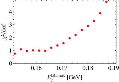
Figure 2: $\chi^{2}_{\textnormal{red}}$ as a function of the fitted energy range from $\pi^{+}$ threshold up to $E_{\gamma}^{\textnormal{lab,max}}$.

In Fig. 2, we show how the $\chi^{2}_{\textnormal{red}}$ changes if one includes all data points up to a maximal energy $E_{\gamma}^{\textnormal{lab,max}}$. It stays around 1 up to bin 8 (bins 1 and 2 corresponding to $E_{\gamma}^{\textnormal{lab}}=147$ MeV and 149.3 MeV, respectively, not shown) and then starts to rise. Furthermore, we took account of the change of the LECs, when including higher energy bins. We decided to take all data up to the first rising bin, namely $E_{\gamma}^{\textnormal{lab}}=165.8$ MeV with $\chi^{2}_{\textnormal{red}}=1.22$. Our results for the LECs, including an error estimate, are shown in Table 2.

Table 2: LECs of the contact diagrams for $\gamma+p\rightarrow p+\pi^{0}$ as obtained from a fit to the data of Ref. Hornidge:2012ca . The $d_{i}$ are given in units of $\textnormal{GeV}^{-2}$ and the $e_{i}$ in units of $\textnormal{GeV}^{-3}$. The errors stem from a bootstrap estimate (see text for details).

LEC	Value
$\tilde{d}_{9}:=d_{8}+d_{9}$	$-2.31\pm 0.02$
$\tilde{e}_{48}:=e_{48}+e_{67}$	$-3.0\pm 0.2$
$\tilde{e}_{49}:=e_{49}+e_{68}$	0
$\tilde{e}_{50}:=e_{50}+e_{69}$	$-1.2\pm 2.1$
$\tilde{e}_{51}:=e_{51}+e_{71}$	$2.3\pm 1.1$
$\tilde{e}_{112}:=e_{112}+e_{113}$	$-4.4\pm 2.1$

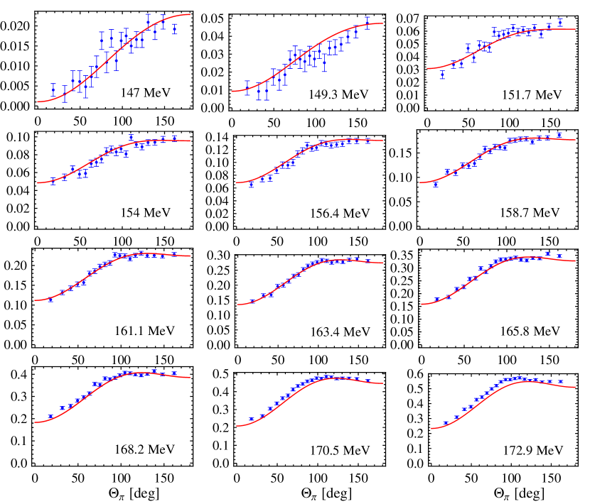
Figure 3: Angular distribution for differential cross sections in $\mu$b/sr for $\gamma+p\rightarrow p+\pi^{0}$. The curves show the results in RChPT at $O(q^{4})$. The data are from Ref. Hornidge:2012ca . The energy $E_{\gamma}^{\textnormal{lab}}$ is given in the panels.

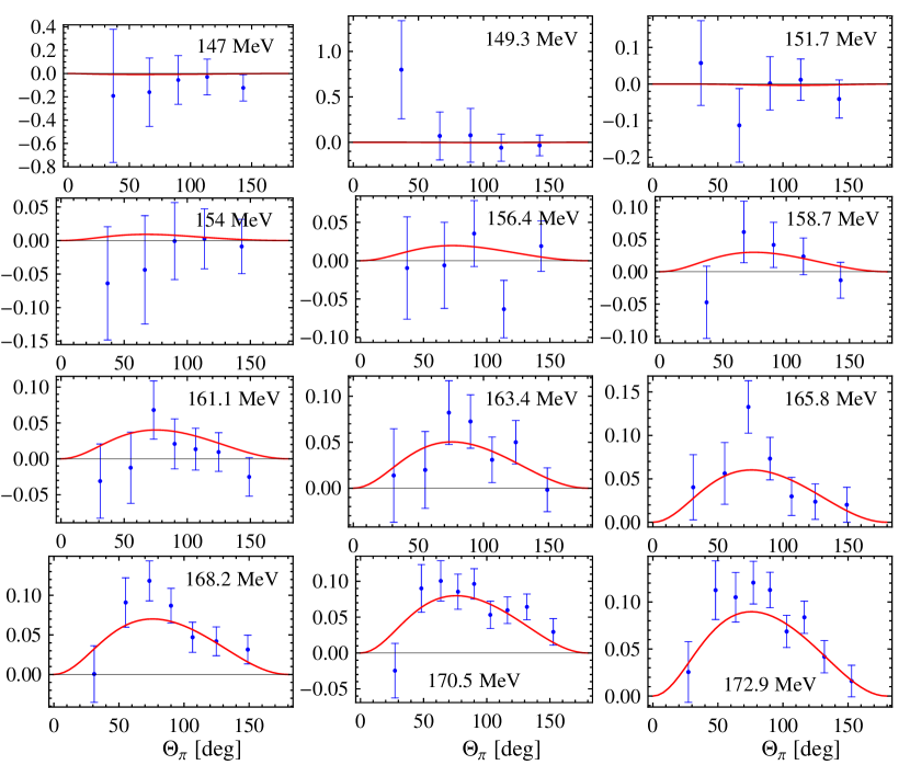
Figure 4: Angular distribution for the polarized photon asymmetries $\Sigma$ for $\gamma+p\rightarrow p+\pi^{0}$. The curves show the results in RChPT at $O(q^{4})$. The data are from Ref. Hornidge:2012ca . The energy $E_{\gamma}^{\textnormal{lab}}$ is given in the panels.

Some exemplary results for the differential cross section and the polarized photon asymmetry are shown in Figs. 3 and 4. In the fitted energy range we get a nice agreement with the data. At higher energies, the calculation starts to deviate from the experiment, because the important $M_{1+}$ multipole, which is dominated by the $\Delta$ resonance, is underestimated. The real parts of the $S$ and $P$ waves are shown in Fig. 5 together with single-energy fits of Ref. Hornidge:2012ca . For comparison, we also show the predictions of the Dubna-Mainz-Taipei (DMT) model Kamalov:2000en ; Kamalov:2001qg and the covariant, unitary, chiral approach of Gasparyan and Lutz (GL) Gasparyan:2010xz .

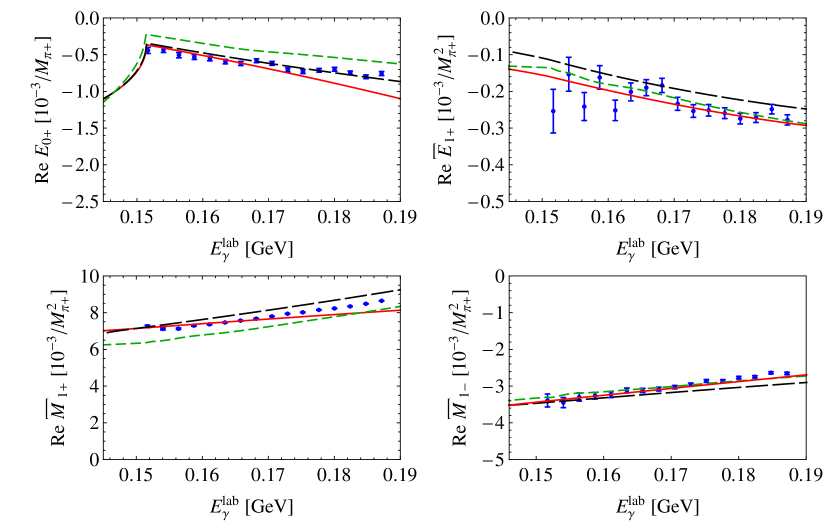
Figure 5: (Color online) $S$- and reduced $P$-wave multipoles for $\gamma+p\rightarrow p+\pi^{0}$. The solid (red) curves show our RChPT calculations at $O(q^{4})$. The short-dashed (green) and long-dashed (black) curves are the predictions of the DMT model Kamalov:2000en ; Kamalov:2001qg and the GL model Gasparyan:2010xz , respectively. The data are from Ref. Hornidge:2012ca .

The multipole $E_{0+}$ agrees nicely with the data in the fitted energy range. The $P$ waves $E_{1+}$ and $M_{1-}$ agree for even higher energies with the single energy fits. The largest deviation can be seen in $M_{1+}$. This multipole is related to the $\Delta$ resonance and the strong rising of the data above 170 MeV can be traced back to the influence of this resonance. As we did not include the $\Delta$ explicitly, this calculation is not able to fully describe its impact on the multipole.

V.2 $\gamma^{*}+p\rightarrow p+\pi^{0}$

After having fixed the LECs of $\pi^{0}$ photoproduction, there remain only two independent structures for electroproduction. We use the latest data of Ref. Merkel:2011cf to determine the corresponding LECs. In Ref. Merkel:2011cf , the differential cross sections $\sigma_{0}=\sigma_{T}+\epsilon\sigma_{L}$ and $\sigma_{LT}$ were precisely measured in the threshold region for different values of $Q^{2}$. We use the same fitting procedure as in photoproduction and also apply the bootstrap method to estimate the errors of the LECs (see Table 3).

Table 3: LECs of the contact diagrams for $\gamma^{\ast}+p\rightarrow p+\pi^{0}$ as obtained from a fit to the data of Ref. Merkel:2011cf . The $e_{i}$ are given in units of $\textnormal{GeV}^{-3}$. The errors stem from a bootstrap estimate (see text for details).

LEC	Value
$\tilde{e}_{52}=e_{52}+e_{72}$	$6.4\pm 0.7$
$\tilde{e}_{53}=e_{53}+e_{73}$	$-0.5\pm 0.2$

We obtain $\chi^{2}_{\textnormal{red}}=1.97$ as the global minimum.

The results for the differential cross sections are shown in Figs. 6 and 7. The calculation agrees nicely with the data. Furthermore, in Fig. 8 we show the total cross section for these energies together with the experimental data Merkel:2009zz ; Merkel:2011cf . Finally, in Fig. 9 we compare our results for the coincidence cross sections $\sigma_{0}$, $\sigma_{TT}$, $\sigma_{LT}$ and the beam asymmetry $A_{LT^{\prime}}$ with the experimental data of Ref. Weis:2007kf and the results of HBChPT Bernard:1996ti and the DMT model Kamalov:2000en ; Kamalov:2001qg .

In general, the DMT model gives a very good description of all observables and amplitudes in the threshold region and can be used as a guideline for theoretical calculations in cases where experimental data do not exist. The HBChPT calculations shown in Fig. 9 were fitted to these data and are taken from Ref. Weis:2007kf . In contrast, our RChPT calculation is not fitted to these data, as all LECs were already determined with the data discussed above. While HBChPT gives a better description for the unpolarized cross section $\sigma_{0}(\Theta_{\pi})=\sigma_{T}(\Theta_{\pi})+\epsilon\sigma_{L}(\Theta_{\pi})$ than our RChPT calculation, a comparison with the separated cross sections $\sigma_{T}$ and $\sigma_{L}$ shows that this is mainly due to a longitudinal cross section which is much too small in the HBChPT fit. For the other observables $\sigma_{LT}$, $\sigma_{TT}$, and the asymmetry $A_{LT^{\prime}}$, RChPT compares much better to the data than HBChPT. It is interesting to note that the asymmetry $A_{LT^{\prime}}$ depends only weakly on LECs and has an important contribution from the parameter-free pion loop contribution.

For the experimental set-up with $\Phi_{\pi}=90^{\circ}$, the asymmetry takes the form [see Eq. (29)]

$$A_{LT^{\prime}}(\Theta_{\pi})=\frac{\sqrt{2\epsilon(1-\epsilon)}\;\sigma_{LT^{\prime}}(\Theta_{\pi})}{\sigma_{T}(\Theta_{\pi})+\epsilon\;\sigma_{L}(\Theta_{\pi})-\epsilon\;\sigma_{TT}(\Theta_{\pi})}\,.$$ (43)

Expanding the observables up to and including $P$ waves, we get at $\Theta_{\pi}=90^{\circ}$

$$A_{LT^{\prime}}(90^{\circ})=\frac{\sqrt{2\epsilon(1-\epsilon)}\;\sqrt{Q^{2}/k_{0}^{2}}\;\mbox{Im}(P_{5}^{*}\,E_{0+}+L_{0+}^{*}\,P_{2})}{|E_{0+}|^{2}+\frac{1}{2}(|P_{3}|^{2}+|P_{2}|^{2})+\epsilon\,(Q^{2}/k_{0}^{2})(|L_{0+}|^{2}+|P_{5}|^{2})-\epsilon\frac{1}{2}(|P_{2}|^{2}-|P_{3}|^{2})}\,,$$ (44)

where $P_{2}=3E_{1+}-M_{1+}+M_{1-}$, $P_{3}=2M_{1+}+M_{1-}$, and $P_{5}=L_{1-}-2L_{1+}$. As a further simplification, we can assume all $P$-wave amplitudes as real numbers, where the magnitudes of $P_{2}$ and $P_{3}$ are much larger than those of all other multipoles. For $\epsilon\approx 1$ we find in very good approximation the simple form

$$A_{LT^{\prime}}(90^{\circ})\approx\frac{\sqrt{2\epsilon(1-\epsilon)}\;\sqrt{Q^{2}/k_{0}^{2}}\;(-P_{2})\;\mbox{Im}(L_{0+})}{P_{3}^{2}}\,.$$ (45)

Therefore, this asymmetry is very sensitive to the imaginary part of the longitudinal $S$ wave $L_{0+}$, hence practically independent of LECs. This is very similar to the case of the target asymmetry $T$ for $\gamma p\to p\pi^{0}$ which we discussed in our previous article Hilt:2013uf . There, the target asymmetry is shown to be the ideal polarization observable to measure $\mbox{Im}(E_{0+})$.

Figure 6: (Color online) Angular distribution for differential cross sections $\sigma_{0}$ in $\mu$b/sr for $\gamma^{*}+p\rightarrow p+\pi^{0}$. The values for the virtual-photon polarization $\epsilon$ are 0.932, 0.882, and 0.829 for increasing $Q^{2}$. The solid (red) curves show our RChPT calculations at $O(q^{4})$. The short-dashed (green) curves are the predictions of the DMT model Kamalov:2000en ; Kamalov:2001qg . The data are from Ref. Merkel:2011cf . The cm energy above threshold $\Delta W$ and the photon virtuality $Q^{2}$ are given in the panels in units of MeV and GeV², respectively.

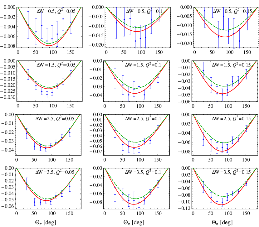
Figure 7: (Color online) Angular distribution for the differential cross sections $\sigma_{LT}$ in $\mu$b/sr for $\gamma^{*}+p\rightarrow p+\pi^{0}$. The curves and the polarization values $\epsilon$ are as in Fig. 6. The data are from Ref. Merkel:2011cf . The cm energy above threshold $\Delta W$ and the photon virtuality $Q^{2}$ are given in the panels in units of MeV and GeV², respectively.

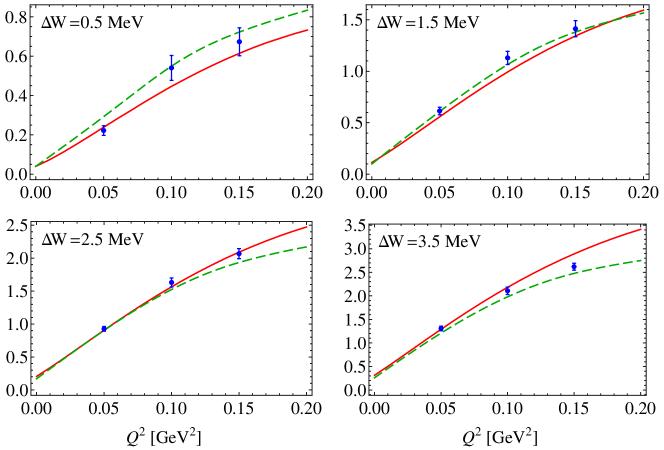
Figure 8: (Color online) Total cross sections in $\mu$b as a function of $Q^{2}$ for different cm energies above threshold $\Delta W$ in MeV. The curves and the polarization values $\epsilon$ are as in Fig. 6. The data are from Refs. Merkel:2009zz ; Merkel:2011cf .

Figure 9: (Color online) Coincidence cross sections $\sigma_{0}$, $\sigma_{TT}$, and $\sigma_{LT}$ in $\mu$b/sr and beam asymmetry $A_{LT^{\prime}}$ in $\%$ at constant $Q^{2}=0.05$ GeV², $\Theta_{\pi}=90^{\circ}$, $\Phi_{\pi}=90^{\circ}$, and $\epsilon=0.93$ as a function of $\Delta W$ above threshold. The solid (red) lines show our RChPT calculations at $O(q^{4})$ and the dotted (black) lines are the heavy-baryon ChPT calculations of Ref. Bernard:1996ti . The dashed (green) curves are obtained from the DMT model Kamalov:2000en ; Kamalov:2001qg . The data are from Ref. Weis:2007kf .

V.3 $\gamma+p\rightarrow n+\pi^{+}$ and $\gamma+n\rightarrow p+\pi^{-}$

We discuss both reaction channels together as we also had to fit them simultaneously. In the production of a $\pi^{0}$ on a proton it is not possible to separate the LECs into their contributions resulting from isospin (0) and (+) amplitudes. In contrast, in the channels involving charged pions one can uniquely determine the LECs in one of the reaction channels alone, as the kinematic structures of the LECs in the ($-$) component differ completely from those of the (0) component. This is ultimately related to the different crossing behavior of Eq. (24) for the different isospin channels.

Strictly speaking, the production of a $\pi^{-}$ on a neutron has never been studied experimentally as there exists no free neutron target. Therefore, one can either study the inverse reaction, namely radiative pion capture, or use, e.g., deuterium as a target. The pion capture cross sections can be completely related to those of pion photoproduction Fearing:2000uy . Here, we focus on all existing data of pion production for both channels as no single experiment contains enough precise data to determine the LECs. We take the world data collected in the data base of the SAID program of Ref. SAID . Besides differential cross sections, there also exist data for the photon asymmetry $\Sigma$, the polarized target asymmetry $T$, and the recoil polarization $P$. For the latter two, the existing data points belong to energies which are very high from the point of view of ChPT. Moreover, these two quantities depend strongly on the imaginary part of the amplitude. Therefore, we cannot describe these data points without including the $\Delta$ resonance and so we do not take them into account.

In the charged channels, the $S$ wave dominates in the threshold region as predicted by the Kroll-Ruderman term Kroll:1953vq . Above threshold, one needs more partial waves to correctly reproduce the full amplitude, as the pion pole enhances higher partial waves. In our fits we therefore use the full CGLN amplitudes to determine the LECs. As before, the procedure relies on multiple fits with random starting values. The errors for the fit parameters are again estimated via the bootstrap method. We also had to estimate the maximum energy to be used for our fit. With the same argument as above, we use $W^{\textnormal{max}}=1160$ MeV, resulting in $\chi^{2}_{\textnormal{red}}=2.39$. In Figs. 10 and 11, we show some exemplary results. For the differential cross sections we find a good agreement with the data up to the highest energies we took into account. The asymmetry $\Sigma$ can also be described quite well over the whole energy range. Only at energies close to the $\Delta$ resonance deviations become visible. Of course, as we have to determine 9 LECs there is some amount of freedom, when fitting the data. In order to illustrate that our results are by no means coincidental, in Fig. 12 we show the $S$- and $P$-wave multipoles of both channels in comparison with the DMT model Kamalov:2000en and the covariant, unitary, chiral approach of GL Gasparyan:2010xz . One can clearly see in the $E_{1+}$ and $M_{1+}$ multipole that we did not include the $\Delta$ resonance explicitly, because the real parts of the multipoles should have a zero crossing at the $\Delta$ resonance position $E_{\gamma}^{\textnormal{lab}}=0.34$ GeV, which is indicated in GL and DMT, as both multipoles start to drop off at the highest energies shown here. The small discrepancies between our calculation and the other two models can be traced back to the data we used. In order to determine $E_{0+}$ and the $P$ waves correctly, one not only needs precise data for the differential cross sections but also for the asymmetry. Here, we only have few data for the asymmetry available and, furthermore, their relative error is bigger compared to the cross sections, which lowers their weight in the fit.

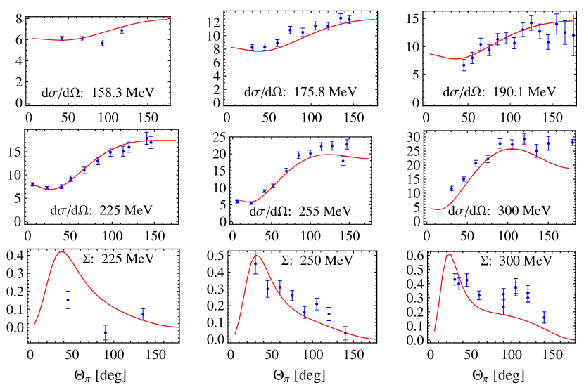
Figure 10: Angular distribution of differential cross sections in $\mu$b/sr and photon asymmetries $\Sigma$ for $\gamma+n\rightarrow p+\pi^{-}$ for different $E_{\gamma}^{\textnormal{lab}}$. The curves show our RChPT calculations at $O(q^{4})$. The data are from Refs. SAID ; Liu:1964bi ; Rossi:1973wf ; Kondo:1974yf ; Ganenko:1976mf ; Fujii:1976jg ; Salomon:1983xn ; Bagheri:1987kf ; Wang:1992 ; Liu:1994 .

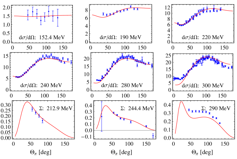
Figure 11: Angular distribution of differential cross sections in $\mu$b/sr and photon asymmetries $\Sigma$ for $\gamma+p\rightarrow n+\pi^{+}$ for different $E_{\gamma}^{\textnormal{lab}}$. The curves show our RChPT calculations at $O(q^{4})$. The data are from Refs. SAID ; Betourne:1968bd ; Fischer:1970df ; Fischer:1972mt ; Fujii:1976jg ; Buechler:1994jg ; Korkmaz:1999sg ; Beck:1999ge ; Branford:1999cp ; Blanpied:2001ae ; Ahrens:2004pf .

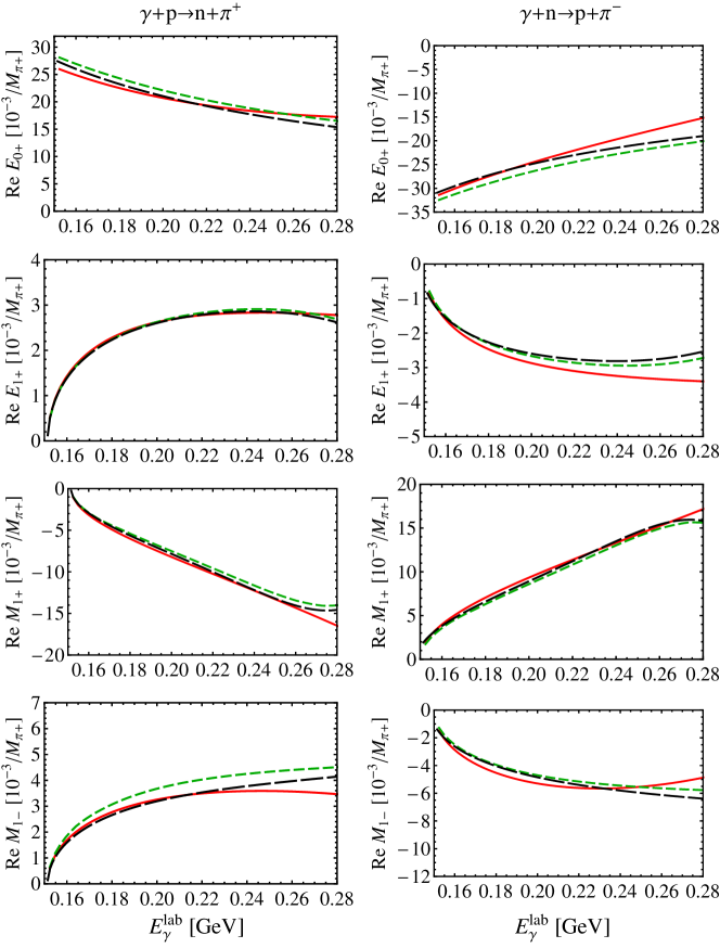
Figure 12: (Color online) $S$- and $P$-wave multipoles for the charged photoproduction channels as a function of $E_{\gamma}^{\textnormal{lab}}$. The solid (red) curves show our RChPT calculations at $O(q^{4})$. The short-dashed (green) and long-dashed (black) curves are the predictions of the DMT model Kamalov:2000en ; Kamalov:2001qg and the GL model Gasparyan:2010xz , respectively.

V.4 $\gamma^{(*)}+p\rightarrow n+\pi^{+}$

In this reaction channel, only a few data points exist in the energy range and for photon virtualities, where ChPT can be applied. Unfortunately, these data of the differential cross sections $\sigma_{T}$ and $\sigma_{L}$ at $W=1125$ MeV are at one fixed angle, namely $\Theta_{\pi}=0^{\circ}$ baumann ; Drechsel:2007sq . Hence, the angular distribution cannot be analyzed. Nevertheless, we use the forward-scattering cross section to fix the two remaining constants through a fit to the data. We refrain from giving an error for these LECs as this is only a first estimate and the amount of data is too small for good statistics. The results of our calculation are shown in Fig. 13. While the theory agrees with the data for $\sigma_{T}$, for $\sigma_{L}$ some deviation is visible.

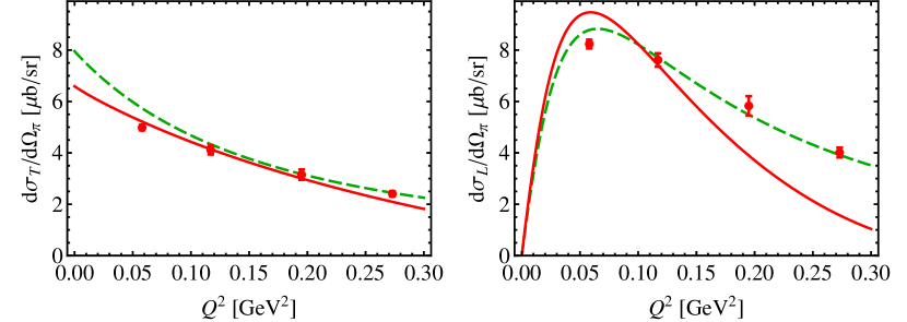
Figure 13: (Color online) Differential cross sections as a function of $Q^{2}$ for $\gamma^{*}+p\rightarrow n+\pi^{+}$ at $W=1125$ MeV and $\Theta_{\pi}=0^{\circ}$. The solid (red) curves show our RChPT calculation at $O(q^{4})$ and the dashed (green) curves are the predictions of the DMT model Kamalov:2000en ; Kamalov:2001qg . The data are from Ref. baumann ; Drechsel:2007sq .

Table 4: Numerical values of all LECs of pion photo- and electroproduction. The $\ast$ indicates constants that appear in electroproduction, only. If possible, the errors were estimated using the bootstrap method (see text for details). In the case of the electroproduction LECs $e_{52}$, $e_{53}$, $e_{72}$, and $e_{73}$ we can only give errors for $\tilde{e}_{52}$ and $\tilde{e}_{53}$ (compare Table 3 and text).

Isospin channel	LEC	Value
0	$d_{9}\ [\textnormal{GeV}^{-2}]$	$-1.22\pm 0.12$
0	$e_{48}\ [\textnormal{GeV}^{-3}]$	$5.2\pm 1.4$
0	$e_{49}\ [\textnormal{GeV}^{-3}]$	$0.9\pm 2.6$
0	$e_{50}\ [\textnormal{GeV}^{-3}]$	$2.2\pm 0.8$
0	$e_{51}\ [\textnormal{GeV}^{-3}]$	$6.6\pm 3.6$
0	$e_{52}^{*}\ [\textnormal{GeV}^{-3}]$	$-4.1$
0	$e_{53}^{*}\ [\textnormal{GeV}^{-3}]$	$-2.7$
0	$e_{112}\ [\textnormal{GeV}^{-3}]$	$9.3\pm 1.6$
+	$d_{8}\ [\textnormal{GeV}^{-2}]$	$-1.09\pm 0.12$
+	$e_{67}\ [\textnormal{GeV}^{-3}]$	$-8.3\pm 1.5$
+	$e_{68}\ [\textnormal{GeV}^{-3}]$	$-0.9\pm 2.6$
+	$e_{69}\ [\textnormal{GeV}^{-3}]$	$-1.0\pm 2.2$
+	$e_{71}\ [\textnormal{GeV}^{-3}]$	$-4.4\pm 3.7$
+	$e_{72}^{*}\ [\textnormal{GeV}^{-3}]$	$10.5$
+	$e_{73}^{*}\ [\textnormal{GeV}^{-3}]$	$2.1$
+	$e_{113}\ [\textnormal{GeV}^{-3}]$	$-13.7\pm 2.6$
$-$	$d_{20}\ [\textnormal{GeV}^{-2}]$	$4.34\pm 0.08$
$-$	$d_{21}\ [\textnormal{GeV}^{-2}]$	$-3.1\pm 0.1$
$-$	$e_{70}\ [\textnormal{GeV}^{-3}]$	$3.9\pm 0.3$

VI Chiral MAID

The complete amplitude at $O(q^{4})$ is a rather lengthy expression and cumbersome to handle. Nevertheless, we wanted to give easy access to anybody who is interested in this calculation. We therefore created $\chi$MAID which is a web interface with certain underlying FORTRAN programs. The main parts of these programs are adopted from MAID2007 Drechsel:2007if . Unfortunately, the computing time for the desired quantities, e.g., cross sections or multipoles, is too high for a web-based application. We avoid calculating the complete amplitude by restricting the input for $\chi$MAID to multipoles up to and including $l=4$ or, in other words, $G$ waves. All observables are derived from the multipoles which we computed beforehand for all reaction channels. The multipoles are calculated for an energy range of $W=1073.3-1190$ MeV and, for electroproduction, through $Q^{2}=0.3\ \textnormal{GeV}^{2}$.

The loop contributions, including their parameters, are fixed and cannot be modified from the outside. On the other hand, the contact diagrams at ${O}(q^{3})$ and ${O}(q^{4})$ enter analytically and the corresponding LECs can be changed arbitrarily (see Table 4 for our present values). This is an important feature in the light of future new experimental data, as more precise data help to get better access to the LECs (see Appendix C).

Of course, $\chi$MAID has a limited range of applicability. First of all, ChPT without additional dynamical degrees of freedom restricts the energy region, where our results can be applied. In the case of neutral pion photoproduction (see Section V.1) one can clearly see that for energies above $E_{\gamma}^{\textnormal{lab}}\approx 170$ MeV the theory starts to deviate from experimental data. In the case of the charged channels the range of applicability is larger, but some observables are quite sensitive to the cutoff of multipoles, as the pion pole term is important at small angles. As an estimate, for $W>1160$ MeV the difference between our full amplitude and the approximation up to and including $G$ waves becomes visible.

VII Summary

We have presented and discussed a full $O(q^{4})$ calculation of pion photo- and electroproduction in the framework of manifestly Lorentz-invariant (relativistic) chiral perturbation theory. By performing fits to the available experimental data, we determined all 19 LECs of the contact graphs at $O(q^{3})$ and $O(q^{4})$ (see Table 4). Our findings can be summarized as follows.

The latest data of Ref. Hornidge:2012ca for $\pi^{0}$ photoproduction on a proton gave us the possibility to determine the $S$ and $P$ waves in the threshold region. The first measurement of the photon asymmetry $\Sigma$ starting from threshold was an important feature of this experiment, because only this way one can access the $S$ and $P$ waves simultaneously. In principle, a sixth LEC exists at $O(q^{4})$ which mainly affects the $E_{2-}$ multipole. Unfortunately, we were not able to pin down this constant and, therefore, neglected it in our fit. Nevertheless, we found a good agreement with the observables and the multipoles up to $E_{\gamma}^{\textnormal{lab}}\approx 170$ MeV.

The experiment of Ref. Merkel:2011cf was utilized to determine the two remaining LECs for $\pi^{0}$ electroproduction on the proton. We found that our results are in good agreement with the available data including the total cross sections. It will be interesting to compare our results with future experiments when further observables can be measured.

In the case of charged pion photoproduction we had to examine both reaction channels simultaneously. None of the existing experiments covered a large enough energy range and, therefore, we decided to use the global data available SAID . The description of the differential cross sections turned out to be satisfactory almost up to the $\Delta$ resonance region. This finding is a little bit misleading as one can clearly see from the results for the asymmetry $\Sigma$, where we find that deviations occur already at somewhat lower energies. Furthermore, the large number of LECs subsume some of the missing imaginary part of the amplitude. This can lead to a wrong picture at the highest energies we took into account, as the missing piece of the imaginary part of the amplitude cannot be included in the LECs.

For charged pion electroproduction we found only one experiment which was suited for an analysis in terms of ChPT baumann ; Drechsel:2007sq . There are only few data points available which, in addition, were measured at a fixed angle, namely in the forward direction. Hence, we consider our analysis only a first estimate. Future experiments will hopefully give us the opportunity to reexamine the two LECs remaining for charged pion electroproduction.

Finally, we presented the web interface $\chi$MAID website . With the estimates for the LECs presented in this article, one can obtain predictions for all desired observables in the threshold region. Therefore, we refrained from showing any additional predictions here. It is clear that new experiments will lead to different estimates for the LECs. For that reason, we included in $\chi$MAID the possibility to change the LECs arbitrarily. This will help to further study the range of validity and applicability of ChPT in the future.

Appendix A Connection between the different sets of amplitudes of pion electroproduction

The connection between the Ball amplitudes $B_{i}$ of Eq. (11) and the invariant amplitudes $A_{i}$ of Eq. (14) can be derived by equating the two parameterizations:

$$\sum_{i=1}^{6}A_{i}M_{i}^{\mu}\stackrel{{\scriptstyle!}}{{=}}\sum_{i=1}^{8}B_{i}V_{i}^{\mu}.$$ (46)

In order to connect the two sets, one can make use of current conservation to eliminate two of the Ball amplitudes [see Eqs. (13)]. By comparing the Lorentz structures, one can read off the following connection [here, we replaced $B_{1}$ and $B_{2}$ by exploiting Eqs. (13)]:

$$\begin{split}A_{1}&=i(B_{5}+m_{N}B_{6}),\\ A_{2}&=-i\frac{k\cdot qB_{3}+k^{2}(B_{4}+B_{5})}{k\cdot P(k^{2}-2k\cdot q)},\\ A_{3}&=iB_{7},\\ A_{4}&=\frac{i}{2}B_{6},\\ A_{5}&=\frac{i}{k^{2}-2k\cdot q}(B_{3}+2B_{4}+2B_{5}),\\ A_{6}&=-iB_{8}.\end{split}$$ (47)

In a similar manner one can relate the invariant amplitudes $A_{i}$ of Eq. (14) to the CGLN amplitudes ${\cal F}_{i}$ of Eq. (19). In the following equations, all (non-invariant) quantities are defined in the cm frame:

$$\begin{split}\mathcal{F}_{1}&=\frac{W-m_{N}}{8\pi W}\sqrt{(E_{i}+m_{N})(E_{f}+m_{N})}\Big{[}A_{1}+(W-m_{N})A_{4}\\ &\quad-\frac{2m_{N}\nu_{B}}{W-m_{N}}(A_{3}-A_{4})+\frac{Q^{2}}{W-m_{N}}A_{6}\Big{]},\\ \mathcal{F}_{2}&=\frac{W+m_{N}}{8\pi W}|\vec{q}\hskip 2.84544pt|\sqrt{\frac{E_{i}-m_{N}}{E_{f}+m_{N}}}\Big{[}-A_{1}+(W+m_{N})A_{4}\\ &\quad-\frac{2m_{N}\nu_{B}}{W+m_{N}}(A_{3}-A_{4})+\frac{Q^{2}}{W+m_{N}}A_{6}\Big{]},\\ \mathcal{F}_{3}&=\frac{W+m_{N}}{8\pi W}|\vec{q}\hskip 2.84544pt|\sqrt{(E_{i}-m_{N})(E_{f}+m_{N})}\left[\frac{2W^{2}-2m_{N}^{2}+Q^{2}}{2(W+m_{N})}A_{2}\right.\\ &\quad\left.+A_{3}-A_{4}-\frac{Q^{2}}{W+m_{N}}A_{5}\right],\\ \mathcal{F}_{4}&=\frac{W-m_{N}}{8\pi W}|\vec{q}\hskip 2.84544pt|^{2}\sqrt{\frac{E_{i}+m_{N}}{E_{f}+m_{N}}}\left[-\frac{2W^{2}-2m_{N}^{2}+Q^{2}}{2(W-m_{N})}A_{2}\right.\\ &\quad\left.+A_{3}-A_{4}+\frac{Q^{2}}{W-m_{N}}A_{5}\right],\\ \mathcal{F}_{5}&=\frac{k_{0}}{8\pi W}\sqrt{\frac{E_{f}+m_{N}}{E_{i}+m_{N}}}\Big{\{}(E_{i}+m_{N})A_{1}\\ &\quad+\left[4m_{N}\nu_{B}\left(W-\frac{3}{4}k_{0}\right)-\vec{k}^{2}W+E_{\pi}\left(W^{2}-m_{N}^{2}+\frac{1}{2}Q^{2}\right)\right]A_{2}\\ &\quad\left.+[E_{\pi}(W+m_{N})+2m_{N}\nu_{B}]A_{3}\right.\\ &\quad+[(E_{i}+m_{N})(W-m_{N})-E_{\pi}(W+m_{N})-2m_{N}\nu_{B}]A_{4}\\ &\quad+(2m_{N}\nu_{B}k_{0}-E_{\pi}Q^{2})A_{5}\\ &\quad-(E_{i}+m_{N})(W-m_{N})A_{6}\Big{\}},\\ \mathcal{F}_{6}&=\frac{k_{0}|\vec{q}\hskip 2.84544pt|}{8\pi W\sqrt{(E_{f}+m_{N})(E_{i}-m_{N})}}\Big{\{}-(E_{i}-m_{N})A_{1}\\ &\quad+\left[\vec{k}^{2}W-4m_{N}\nu_{B}\left(W-\frac{3}{4}k_{0}\right)-E_{\pi}\left(W^{2}-m_{N}^{2}+\frac{1}{2}Q^{2}\right)\right]A_{2}\\ &\quad+[E_{\pi}(W-m_{N})+2m_{N}\nu_{B}]A_{3}\\ &\quad+[(E_{i}-m_{N})(W+m_{N})-E_{\pi}(W-m_{N})-2m_{N}\nu_{B}]A_{4}\\ &\quad+(E_{\pi}Q^{2}-2m_{N}\nu_{B}k_{0})A_{5}\\ &\quad-(E_{i}-m_{N})(W+m_{N})A_{6}\Big{\}},\end{split}$$ (48)

where $2\nu_{B}=-k\cdot q$.

Appendix B differential cross sections

In order to describe the individual parts of the differential cross section, the so-called response functions are commonly used Drechsel:1992pn :

$$\begin{split}R_{T}&=|F_{1}|^{2}+|F_{2}|^{2}+\frac{1}{2}\sin^{2}{\Theta_{\pi}}\left(|F_{3}|^{2}+|F_{4}|^{2}\right)\\ &\quad-\textnormal{Re}\left[2\cos\Theta_{\pi}F_{1}^{*}F_{2}-\sin^{2}\Theta_{\pi}(F_{1}^{*}F_{4}+F_{2}^{*}F_{3}+\cos\Theta_{\pi}F_{3}^{*}F_{4})\right],\\ R_{L}&=|F_{5}|^{2}+|F_{6}|^{2}+2\cos\Theta_{\pi}\textnormal{Re}\left(F_{5}^{*}F_{6}\right),\\ R_{LT}&=-\sin\Theta_{\pi}\textnormal{Re}\left[(F_{2}^{*}+F_{3}^{*}+\cos\Theta_{\pi}F_{4}^{*})F_{5}+(F_{1}^{*}+F_{4}^{*}+\cos\Theta_{\pi}F_{3}^{*})F_{6}\right],\\ R_{TT}&=\sin^{2}\Theta_{\pi}\left[\frac{1}{2}(|F_{3}|^{2}+|F_{4}|^{2})+\textnormal{Re}\left(F_{1}^{*}F_{4}+F_{2}^{*}F_{3}+\cos\Theta_{\pi}F_{3}^{*}F_{4}\right)\right],\\ R_{LT^{\prime}}&=-\sin\Theta_{\pi}\textnormal{Im}\left[(F_{2}^{*}+F_{3}^{*}+\cos\Theta_{\pi}F_{4}^{*})F_{5}+(F_{1}^{*}+F_{4}^{*}+\cos\Theta_{\pi}F_{3}^{*})F_{6}\right].\end{split}$$ (49)

All other parts of the differential cross section are not relevant for the discussions in this article. They can be found in Ref. Drechsel:1992pn . The connection between the response functions and the cross sections reads

$$\begin{split}\frac{d\sigma_{T}}{d\Omega_{\pi}}&=\frac{|\vec{q}|}{k_{\gamma}^{\textnormal{cm}}}R_{T},\\ \frac{d\sigma_{L}}{d\Omega_{\pi}}&=\frac{|\vec{q}|}{k_{\gamma}^{\textnormal{cm}}}\frac{Q^{2}}{k_{0}^{2}}R_{L},\\ \frac{d\sigma_{LT}}{d\Omega_{\pi}}&=\frac{|\vec{q}|}{k_{\gamma}^{\textnormal{cm}}}\frac{Q}{|k_{0}|}R_{LT},\\ \frac{d\sigma_{TT}}{d\Omega_{\pi}}&=\frac{|\vec{q}|}{k_{\gamma}^{\textnormal{cm}}}R_{TT},\\ \frac{d\sigma_{LT^{\prime}}}{d\Omega_{\pi}}&=\frac{|\vec{q}|}{k_{\gamma}^{\textnormal{cm}}}\frac{Q}{|k_{0}|}R_{LT^{\prime}},\end{split}$$ (50)

where $k_{\gamma}^{\textnormal{cm}}=k_{\gamma}m_{N}/W$ is the photon equivalent energy in the cm frame. Furthermore, several polarization observables can be derived. Here, we only need the photon asymmetry,

$$\Sigma=-R_{TT}/R_{T}.$$ (51)

It appears in the case of polarized photons, as the differential cross section $d\sigma/d\Omega_{\pi}$ in the cm frame then gets modulated depending on the angle $\phi$ between the polarization vector of the photon and the reaction plane spanned by the nucleon and pion three momenta:

$$\frac{d\sigma}{d\Omega_{\pi}}(\Theta_{\pi},\phi)=\frac{d\sigma}{d\Omega_{\pi}}(\Theta_{\pi})\left[1-\Sigma(\Theta_{\pi})\cos(2\phi)\right].$$ (52)

Appendix C Making new estimates for LECs

If one is interested in analyzing new experiments and re-estimating the LECs, one can proceed as follows. By switching off the LECs on the $\chi$MAID web page, one gets any desired amplitude or the multipoles with $l\leq 2$ numerically. One can then add the analytic expressions for the contact diagrams given below. From that one can calculate any desired observable and make estimates for the LECs. We give the results for the invariant amplitudes, as they are in a very compact form. The results for the $O(q^{3})$ contact diagrams read

$$\begin{split}A_{1}^{(0)}&=-\frac{2ed_{9}t}{Fm},\\ A_{2}^{(0)}&=-\frac{2ed_{9}\left(k^{2}-M^{2}+t\right)}{Fm\left(M^{2}-t\right)},\\ A_{3}^{(0)}&=0,\\ A_{4}^{(0)}&=-\frac{4ed_{9}}{F},\\ A_{5}^{(0)}&=\frac{ed_{9}(s-u)}{Fm\left(M^{2}-t\right)},\\ A_{6}^{(0)}&=0,\\ A_{1}^{(-)}&=\frac{ed_{20}(s-u)}{4Fm},\\ A_{2}^{(-)}&=0,\\ A_{3}^{(-)}&=-\frac{ed_{20}\left(k^{2}-M^{2}-t\right)}{8Fm^{2}}+\frac{ed_{21}}{F},\\ A_{4}^{(-)}&=\frac{ed_{20}(s-u)}{8Fm^{2}},\\ A_{5}^{(-)}&=0,\\ A_{6}^{(-)}&=-\frac{ed_{20}\left(k^{2}-M^{2}-t\right)}{8Fm^{2}}.\end{split}$$ (53)

The results for the (+) components can be derived from the (0) components by replacing $d_{9}\rightarrow d_{8}$. From a practical point of view, one may replace $m$, $F$, and $M^{2}$ by their physical values $m_{N}$, $F_{\pi}$, and $M_{\pi}^{2}$, as the consequences for the pion production amplitude are of higher order in the chiral expansion. For the $O(q^{4})$ contact diagrams the results read

$$\begin{split}A_{1}^{(0)}&=-e(2e_{49}-e_{51})\frac{k^{2}+M^{2}-t}{2F}\\ &\quad-\frac{ee_{50}}{6Fm^{2}}\left\{2M^{4}+\left[4m^{2}-2(s+u)\right]M^{2}+2m^{4}+s^{2}+u^{2}-2m^{2}(s+u)\right\}\\ &\quad+ee_{52}\frac{k^{2}}{F}-2ee_{112}\frac{M^{2}}{F},\\ A_{2}^{(0)}&=-\frac{2ee_{49}\left(k^{2}+M^{2}-t\right)}{F\left(M^{2}-t\right)}+\frac{2ee_{52}k^{2}}{F\left(M^{2}-t\right)},\\ A_{3}^{(0)}&=e(e_{48}+e_{49})\frac{s-u}{2Fm}+ee_{50}\frac{(k^{2}-M^{2}-t)(s-u)}{12Fm^{3}},\\ A_{4}^{(0)}&=-e(2e_{49}-e_{51})\frac{k^{2}+M^{2}-t}{4Fm}\\ &\quad-\frac{ee_{50}}{12Fm^{3}}\left\{2M^{4}+\left[4m^{2}-2(s+u)\right]M^{2}+2m^{4}+s^{2}+u^{2}-2m^{2}(s+u)\right\}\\ &\quad+ee_{52}\frac{k^{2}}{2Fm}-ee_{112}\frac{M^{2}}{Fm},\\ A_{5}^{(0)}&=\frac{e\left(e_{49}-e_{52}\right)(s-u)}{F\left(M^{2}-t\right)},\\ A_{6}^{(0)}&=\frac{ee_{50}\left(k^{2}-M^{2}-t\right)(s-u)}{12Fm^{3}}+\frac{e\left(e_{52}+e_{53}\right)(s-u)}{4Fm},\\ A_{1}^{(-)}&=-\frac{ee_{70}t(s-u)}{Fm^{2}},\\ A_{2}^{(-)}&=-\frac{ee_{70}\left(k^{2}-M^{2}+t\right)(s-u)}{Fm^{2}\left(M^{2}-t\right)},\\ A_{3}^{(-)}&=0,\\ A_{4}^{(-)}&=-\frac{2ee_{70}(s-u)}{Fm},\\ A_{5}^{(-)}&=\frac{ee_{70}(s-u)^{2}}{2Fm^{2}\left(M^{2}-t\right)},\\ A_{6}^{(-)}&=0.\end{split}$$ (54)

Again, the expressions for the (+) components follow from the (0) components by making the following replacements:

$$e_{48} \rightarrow e_{67},$$

$$e_{49} \rightarrow e_{68},$$

$$e_{50} \rightarrow e_{69},$$

$$e_{51} \rightarrow e_{71},$$

$$e_{52} \rightarrow e_{72},$$

$$e_{53} \rightarrow e_{73},$$

$$e_{112} \rightarrow e_{113}.$$

Moreover, $m$, $F$, and $M^{2}$ may be replaced by their physical values.

References

• (1) H. Yukawa, Proc. Phys. Math. Soc. Jap.  17, 48 (1935).
• (2) E. Epelbaum, H.-W. Hammer, and U.-G. Meißner, Rev. Mod. Phys.  81, 1773 (2009).
• (3) R. Machleidt and D. R. Entem, Phys. Rept.  503, 1 (2011).
• (4) C. M. G. Lattes, H. Muirhead, G. P. S. Occhialini, and C. F. Powell, Nature 159, 694 (1947).
• (5) E. Gardner and C. M. G. Lattes, Science 107, 270 (1948).
• (6) J. Burfening, E. Gardner, and C. M. G. Lattes, Phys. Rev.  75, 382 (1949).
• (7) R. Bjorklund, W. E. Crandall, B. J. Moyer, and H. F. York, Phys. Rev.  77, 213 (1950).
• (8) J. Steinberger, W. K. H. Panofsky, and J. Steller, Phys. Rev.  78, 802 (1950).
• (9) N. M. Kroll and M. A. Ruderman, Phys. Rev.  93, 233 (1954).
• (10) G. F. Chew, M. L. Goldberger, F. E. Low, and Y. Nambu, Phys. Rev.  106, 1345 (1957).
• (11) P. Dennery, Phys. Rev.  124, 2000 (1961).
• (12) O. Hanstein, D. Drechsel, and L. Tiator, Phys. Lett. B 399, 13 (1997).
• (13) O. Hanstein, D. Drechsel, and L. Tiator, Nucl. Phys. A 632, 561 (1998).
• (14) S. S. Kamalov, L. Tiator, D. Drechsel, R. A. Arndt, C. Bennhold, I. I. Strakovsky, and R. L. Workman, Phys. Rev. C 66, 065206 (2002).
• (15) B. Pasquini, D. Drechsel, and L. Tiator, Eur. Phys. J. A 23, 279 (2005).
• (16) B. Pasquini, D. Drechsel, and L. Tiator, Eur. Phys. J. A 27, 231 (2006).
• (17) B. Pasquini, D. Drechsel, and L. Tiator, Eur. Phys. J. A 34, 387 (2007).
• (18) D. Drechsel, B. Pasquini, and L. Tiator, Few-Body Syst.  41, 13 (2007).
• (19) Y. Nambu, Phys. Rev. Lett.  4, 380 (1960).
• (20) Y. Nambu and G. Jona-Lasinio, Phys. Rev.  122, 345 (1961); 124, 246 (1961).
• (21) J. Goldstone, Nuovo Cim.  19, 154 (1961).
• (22) J. Goldstone, A. Salam, and S. Weinberg, Phys. Rev.  127, 965 (1962).
• (23) Y. Nambu and D. Lurie, Phys. Rev.  125, 1429 (1962).
• (24) Y. Nambu and E. Shrauner, Phys. Rev.  128, 862 (1962).
• (25) S. L. Adler and R. F. Dashen, Current Algebras and Applications to Particle Physics (Benjamin, New York, 1968).
• (26) S. Treiman, R. Jackiw, and D. J. Gross, Lectures on Current Algebra and Its Applications (Princeton University Press, Princeton, 1972).
• (27) V. de Alfaro, S. Fubini, G. Furlan, and C. Rossetti, Currents in Hadron Physics (North-Holland, Amsterdam, 1973).
• (28) M. Gell-Mann, Phys. Rev.  125, 1067 (1962).
• (29) J. Bernstein, M. Gell-Mann, and L. Michel, Nuovo Cim. 16, 560 (1960).
• (30) M. Gell-Mann and M. Lévy, Nuovo Cim.  16, 705 (1960).
• (31) J. Bernstein, S. Fubini, M. Gell-Mann, and W. Thirring, Nuovo Cim. 17, 757 (1960).
• (32) S. Fubini, G. Furlan, and C. Rossetti, Nuovo Cim. 40, 1171 (1965).
• (33) V. Bernard, B. Kubis, and U.-G. Meißner, Eur. Phys. J. A 25, 419 (2005).
• (34) S. L. Adler and F. J. Gilman, Phys. Rev.  152, 1460 (1966).
• (35) T. Fuchs and S. Scherer, Phys. Rev. C 68, 055501 (2003).
• (36) P. De Baenst, Nucl. Phys. B 24, 633 (1970).
• (37) A. I. Vainshtein and V. I. Zakharov, Nucl. Phys. B 36, 589 (1972).
• (38) S. Scherer and J. H. Koch, Nucl. Phys. A 534, 461 (1991).
• (39) E. Amaldi, S. Fubini, and G. Furlan, Springer Tracts Mod. Phys.  83, 1 (1979).
• (40) S. Weinberg, Phys. Rev. Lett.  18, 188 (1967).
• (41) J. S. Schwinger, Phys. Lett. B 24, 473 (1967).
• (42) S. Weinberg, Phys. Rev.  166, 1568 (1968).
• (43) S. R. Coleman, J. Wess, and B. Zumino, Phys. Rev.  177, 2239 (1969).
• (44) C. G. Callan, Jr., S. R. Coleman, J. Wess, and B. Zumino, Phys. Rev.  177, 2247 (1969).
• (45) S. Weinberg, Physica A 96, 327 (1979).
• (46) J. Gasser and H. Leutwyler, Annals Phys.  158, 142 (1984).
• (47) J. Gasser, M. E. Sainio, and A. Švarc, Nucl. Phys. B 307, 779 (1988).
• (48) G. Ecker, Prog. Part. Nucl. Phys.  35, 1 (1995).
• (49) V. Bernard, N. Kaiser, and U.-G. Meißner, Int. J. Mod. Phys. E 4, 193 (1995).
• (50) S. Scherer, Adv. Nucl. Phys.  27, 277 (2003).
• (51) S. Scherer and M. R. Schindler, Lect. Notes Phys.  830, 1 (2012).
• (52) M. I. Adamovich, Proc. P. N. Lebedev Physics Institute 71, 119 (1976).
• (53) E. Mazzucato et al., Phys. Rev. Lett.  57, 3144 (1986).
• (54) R. Beck et al., Phys. Rev. Lett.  65, 1841 (1990).
• (55) V. Bernard, N. Kaiser, J. Gasser, and U.-G. Meißner, Phys. Lett. B 268, 291 (1991).
• (56) R. M. Davidson, Phys. Rev. C 47, 2492 (1993).
• (57) T. P. Welch et al., Phys. Rev. Lett.  69, 2761 (1992).
• (58) M. Wang, PhD thesis, University of Kentucky, 1992.
• (59) K. Liu, Radiative $\pi^{-}p$ capture and the low energy theorem, PhD thesis, University of Kentucky, 1994.
• (60) H. B. van den Brink et al., Phys. Rev. Lett.  74, 3561 (1995).
• (61) K. I. Blomqvist et al., Z. Phys. A 353, 415 (1996).
• (62) M. Fuchs et al., Phys. Lett. B 368, 20 (1996).
• (63) J. C. Bergstrom, J. M. Vogt, R. Igarashi, K. J. Keeter, E. L. Hallin, G. A. Retzlaff, D. M. Skopik, and E. C. Booth, Phys. Rev. C 53, 1052 (1996).
• (64) A. M. Bernstein, E. Shuster, R. Beck, M. Fuchs, B. Krusche, H. Merkel, and H. Ströher, Phys. Rev. C 55, 1509 (1997).
• (65) J. C. Bergstrom, R. Igarashi, and J. M. Vogt, Phys. Rev. C 55, 2016 (1997).
• (66) M. A. Kovash [E643 Collaboration], PiN Newslett.  12N3, 51 (1997).
• (67) J. C. Bergstrom, Phys. Rev. C 58, 2574 (1998).
• (68) M. O. Distler et al., Phys. Rev. Lett.  80, 2294 (1998).
• (69) A. Liesenfeld et al. [A1 Collaboration], Phys. Lett. B 468, 20 (1999).
• (70) E. Korkmaz et al., Phys. Rev. Lett.  83, 3609 (1999).
• (71) A. Schmidt et al., Phys. Rev. Lett.  87, 232501 (2001) [Erratum-ibid.  110, 039903 (2013)].
• (72) H. Merkel et al., Phys. Rev. Lett.  88, 012301 (2002).
• (73) D. Baumann, $\pi^{+}$-Elektroproduktion an der Schwelle, PhD thesis (in German), JGU Mainz, 2005, [http://ubm.opus.hbz-nrw.de/volltexte/2006/923/pdf/diss.pdf].
• (74) M. Weis et al. [A1 Collaboration], Eur. Phys. J. A 38, 27 (2008).
• (75) H. Merkel, PoS CD 09, 112 (2009).
• (76) H. Merkel et al., arXiv:1109.5075 [nucl-ex].
• (77) D. Hornidge et al. [A2 and CB-TAPS Collaboration], Phys. Rev. Lett.  111, 062004 (2013).
• (78) D. Hornidge, PoS CD 12, 070 (2013).
• (79) R. Lindgren et al. [Hall A Collaboration], PoS CD 12, 073 (2013).
• (80) V. Bernard, N. Kaiser, J. Kambor, and U.-G. Meißner, Nucl. Phys. B 388, 315 (1992).
• (81) V. Bernard, N. Kaiser, and U.-G. Meißner, Nucl. Phys. B 383, 442 (1992).
• (82) V. Bernard, N. Kaiser, and U.-G. Meißner, Phys. Rev. Lett.  69, 1877 (1992).
• (83) V. Bernard, N. Kaiser, T. S. H. Lee, and U.-G. Meißner, Phys. Rept.  246, 315 (1994).
• (84) V. Bernard, N. Kaiser, and U.-G. Meißner, Phys. Rev. Lett.  74, 3752 (1995).
• (85) V. Bernard, N. Kaiser, and U.-G. Meißner, Z. Phys. C 70, 483 (1996).
• (86) V. Bernard, N. Kaiser, and U.-G. Meißner, Phys. Lett. B 378, 337 (1996).
• (87) V. Bernard, N. Kaiser, and U.-G. Meißner, Phys. Lett. B 383, 116 (1996).
• (88) V. Bernard, N. Kaiser, and U.-G. Meißner, Nucl. Phys. A 607, 379 (1996) [Erratum-ibid. A 633, 695 (1998)].
• (89) H. W. Fearing, T. R. Hemmert, R. Lewis, and C. Unkmeir, Phys. Rev. C 62, 054006 (2000).
• (90) V. Bernard, N. Kaiser, and U.-G. Meißner, Eur. Phys. J. A 11, 209 (2001).
• (91) C. Fernandez-Ramirez and A. M. Bernstein, Phys. Lett. B 724, 253 (2013).
• (92) T. Becher and H. Leutwyler, Eur. Phys. J. C 9, 643 (1999).
• (93) J. Gegelia and G. Japaridze, Phys. Rev.  D 60, 114038 (1999).
• (94) T. Fuchs, J. Gegelia, G. Japaridze, and S. Scherer, Phys. Rev. D 68, 056005 (2003).
• (95) T. Becher and H. Leutwyler, JHEP 0106, 017 (2001).
• (96) Y.-H. Chen, D.-L. Yao, and H. Q. Zheng, Phys. Rev. D 87, 054019 (2013).
• (97) J. M. Alarcon, J. Martin Camalich, and J. A. Oller, Annals Phys.  336, 413 (2013).
• (98) M. Hilt, S. Scherer, and L. Tiator, Phys. Rev. C 87, 045204 (2013).
• (99) Chiral MAID, [http://www.kph.uni-mainz.de/MAID/chiralmaid/].
• (100) J. S. Ball, Phys. Rev.  124, 2014 (1961).
• (101) D. Drechsel and L. Tiator, J. Phys. G 18, 449 (1992).
• (102) S. L. Adler, Annals Phys.  50, 189 (1968).
• (103) R. M. Davidson, Czech. J. Phys.  44, 365 (1995).
• (104) T. R. Hemmert, B. R. Holstein, and J. Kambor, J. Phys. G 24, 1831 (1998).
• (105) C. Hacker, N. Wies, J. Gegelia, and S. Scherer, Phys. Rev. C 72, 055203 (2005).
• (106) V. Pascalutsa and M. Vanderhaeghen, Phys. Rev. D 73, 034003 (2006).
• (107) B. Kubis and U.-G. Meißner, Nucl. Phys. A 679, 698 (2001).
• (108) M. R. Schindler, J. Gegelia, and S. Scherer, Eur. Phys. J. A 26, 1 (2005).
• (109) M. R. Schindler, T. Fuchs, J. Gegelia, and S. Scherer, Phys. Rev. C 75, 025202 (2007).
• (110) T. Bauer, J. C. Bernauer, and S. Scherer, Phys. Rev. C 86, 065206 (2012).
• (111) G. Colangelo, J. Gasser, and H. Leutwyler, Phys. Rev. Lett.  86, 5008 (2001).
• (112) G. Ecker and M. Mojžiš, Phys. Lett.  B 365, 312 (1996).
• (113) N. Fettes, U.-G. Meißner, M. Mojžiš, and S. Steininger, Annals Phys.  283, 273 (2000) [Erratum-ibid.  288, 249 (2001)].
• (114) R. Mertig, M. Bohm, and A. Denner, Comput. Phys. Commun.  64, 345 (1991).
• (115) T. Hahn, Comput. Phys. Commun.  140, 418 (2001).
• (116) J. Beringer et al. [Particle Data Group Collaboration], Phys. Rev. D 86, 010001 (2012).
• (117) J. Bijnens, G. Colangelo, and P. Talavera, JHEP 9805, 014 (1998).
• (118) H. Merkel, private communication.
• (119) H. C. Schröder et al., Eur. Phys. J. C 21, 473 (2001).
• (120) V. Baru, C. Hanhart, M. Hoferichter, B. Kubis, A. Nogga, and D. R. Phillips, Phys. Lett. B 694, 473 (2011).
• (121) G. Fäldt, Nucl. Phys. A 333, 357 (1980).
• (122) A. M. Bernstein, Phys. Lett. B 442, 20 (1998).
• (123) B. Efron and R. J. Tibshirani, An Introduction to the Bootstrap (Chapman & Hall/CRC, Boca Raton, FL, 1993).
• (124) C. Fernandez-Ramirez, A. M. Bernstein, and T. W. Donnelly, Phys. Lett.  B 679, 41 (2009).
• (125) C. Fernandez-Ramirez, A. M. Bernstein, and T. W. Donnelly, Phys. Rev. C 80, 065201 (2009).
• (126) S. S. Kamalov, S. N. Yang, D. Drechsel, O. Hanstein, and L. Tiator, Phys. Rev. C 64, 032201 (2001).
• (127) S. S. Kamalov, G.-Y. Chen, S.-N. Yang, D. Drechsel, and L. Tiator, Phys. Lett. B 522, 27 (2001).
• (128) A. Gasparyan and M. F. M. Lutz, Nucl. Phys. A 848, 126 (2010).
• (129) Center for Nuclear Studies, Data Analysis Center, SAID program,
[http://gwdac.phys.gwu.edu/].
• (130) F. F. Liu, D. J. Drickey, and R. F. Mozley, Phys. Rev.  136, B1183 (1964).
• (131) V. Rossi et al., Nuovo Cim. A 13, 59 (1973).
• (132) K. Kondo et al., Phys. Rev. D 9, 529 (1974).
• (133) V. B. Ganenko et al., Sov. J. Nucl. Phys.  23, 511 (1976).
• (134) T. Fujii et al., Nucl. Phys. B 120, 395 (1977).
• (135) M. Salomon, D. F. Measday, J. M. Poutissou, and B. C. Robertson, Nucl. Phys. A 414, 493 (1984).
• (136) A. Bagheri, K. A. Aniol, F. Entezami, M. D. Hasinoff, D. F. Measday, J. M. Poutissou, M. Salomon, and B. C. Robertson, Phys. Rev. C 38, 875 (1988).
• (137) C. Betourne, J. C. Bizot, J. P. Perez-y-Jorba, D. Treille, and W. Schmidt, Phys. Rev.  172, 1343 (1968).
• (138) G. Fischer, H. Fischer, M. Heuel, G. Von Holtey, G. Knop, and J. Stümpfig, Nucl. Phys. B 16, 119 (1970).
• (139) G. Fischer, G. Von Holtey, G. Knop, and J. Stümpfig, Z. Phys.  253, 38 (1972).
• (140) K. Büchler et al., Nucl. Phys. A 570, 580 (1994).
• (141) R. Beck et al., Phys. Rev. C 61, 035204 (2000).
• (142) D. Branford et al., Phys. Rev. C 61, 014603 (2000).
• (143) G. Blanpied et al., Phys. Rev. C 64, 025203 (2001).
• (144) J. Ahrens et al. [GDH and A2 Collaboration], Eur. Phys. J. A 21, 323 (2004).
• (145) D. Drechsel and T. Walcher, Rev. Mod. Phys.  80, 731 (2008).
• (146) D. Drechsel, S. S. Kamalov, and L. Tiator, Eur. Phys. J. A 34, 69 (2007).