Mechanical control of heat conductivity in microscopic models of dielectrics

Abstract

We discuss a possibility to control a heat conductivity in simple one-dimensional models of dielectrics by means of external mechanical loads. To illustrate such possibilities we consider first a well-studied chain with degenerate double-well potential of the interparticle interaction. Contrary to previous studies, we consider varying length of the chain with fixed number of particles. Number of possible energetically degenerate ground states strongly depends on the overall length of the chain, or, in other terms, on average length of the link between neighboring particles. These degenerate states correspond to mechanical equilibrium, therefore one can say that the transition between them mimics to some extent a process of plastic deformation. We demonstrate that such modification of the chain length can lead to quite profound (almost five-fold) reduction of the heat conduction coefficient. Even more profound effect is revealed for a model with single-well non-convex potential. It is demonstrated that in certain range of constant external forcing this model becomes ”effectively” double-well, and has a multitude of possible states of equilibrium for the same value of the external load. Thus, the heat conduction coefficient can be reduced by two orders of magnitude. We suggest a mechanical model of a chain with periodic double-well potential, which allows control over the heat conduction. The models considered may be useful for description of heat transport in biological macromolecules and for control of the heat transport in microsystems.

I Introduction

Heat conduction in low-dimensional systems has attracted a lot of attention and has been a subject of intensive studies LLP03 . The main objective here is to derive from first principles (on the atomic-molecular level) the Fourier law – proportionality of the heat flux to the temperature gradient $J=-\kappa\nabla T$, where $\kappa$ is the heat conduction coefficient. To date, there exists quite extensive body of works devoted to the numerical modeling of the heat transfer in the one-dimensional chains. Anomalous characteristics of this process are well-known since celebrated work of Fermi, Pasta and Ulam FPU . In integrable systems (harmonic chain, Toda lattice, the chain of rigid disks) the heat flux $J$ does not depend at all on the chain length $L$, therefore, the thermal conductivity formally diverges. The underlying reason for that is that the energy is transferred by non-interacting quasiparticles and therefore one cannot expect any diffusion effects. Non-integrability of the system is a necessary but not sufficient condition to obtain the convergent heat conduction coefficient. Well-known examples are Fermi-Pasta-Ulam (FPU) chainLRP ; LLP1 ; LLP2 , disordered harmonic chain RG ; CL ; D , diatomic 1D gas of colliding particles D1 ; STZ02 ; GNY and the diatomic Toda lattice H . In these non-integrable systems also have divergent heat conduction coefficient; the latter diverges as a power function of length: $\kappa\sim L^{\alpha}$, for $L\rightarrow\infty$. The exponent lies in the interval $0<\alpha<1$.

On the other side, the 1D lattice with on-site potential can have finite conductivity. The simulations had demonstrated the convergence of the heat conduction coefficient for Frenkel-Kontorova chain HLZ98 ; SG03 , the chain with hyperbolic sine on-site potential TBSZ , the chain with $\phi^{4}$ on-site potential HLZ00 ; AK00 and for the chain of hard disks of non-zero size with substrate potential GS04 . The essential feature of all these models is existence of an external potential modeling the interaction with the surrounding system. These systems are not translationally invariant, and, consequently, the total momentum is not conserved. In paper H it has been suggested that the presence of an external potential plays a key role to ensure the convergence of the heat conductivity. This hypothesis has been disproved in works giardina ; savin2 , where it was shown that the isolated chain of rotators (a chain with a periodic potential interstitial interaction) has a finite thermal conductivity. In recent studies ZZWZ12 ; CZWZ12 it was demonstrated that the heat conduction is convergent even in a chain with Morse potential of the nearest-neighbor interaction. It seems that this finding is intimately related to the fact that the ”extension” branch of the potential function is finite – in other terms, a dissociation of the neighboring particles is possible SK13 . Thus, the heat flux is scattered on these fluctuating large gaps between the fragments of the chain.

In the systems mentioned above, the strong non-homogeneities, which critically effect the heat transfer, are caused by the thermal fluctuations. In current work, we would like to explore somewhat different idea – to design the interaction potential and external conditions in a way that the inhomogeneities will appear in controllable manner and with desired density. Thus, it might be possible to control the heat conduction coefficient in wide range by simple variation of the external conditions – for instance, by stretching the chain. In order to accomplish this goal, we study a chain with a double-well (DW) potential of the nearest-neighbor interactions. We also study certain modification of the DW model, which has only one minimum but can acquire the double-well structure under action of external force. These systems are studied both under nonequilibrium conditions using Langevin thermostats, and within the framework of equilibrium molecular dynamics using Green-Kubo formula GK .

In the first time the thermal conductivity of the chain with double-well potential was considered in giardina , with the of help nonequilibrium molecular-dynamics simulation with Nose-Hoover thermostats. It was shown that the use of Nose-Hoover thermostat for the non-equilibrium problems can be misleading FHLZ ; LLM . More accurate modeling of the heat transfer using c Langevin thermostat was presented in Roy .

It seems that neither of these previous works considered the relationship between the variations of the chain length and the thermal conductivity. However, an important feature of the chain with the DW potential is the existence of a large number of possible ground states of the chain. So, the chain with $N$ particles and periodic boundary conditions has $2^{N-1}$ possible ground states with the same energy; the only possible difference between these states is the overall equilibrium length of the chain. We show that the thermal conductivity of the chain depends essentially on its ground state, governed by the length. In each particular simulation, the overall length of the chain is fixed, and all ground states corresponding to this particular value of the length are considered to be equivalent. So, we are going to show that a variation of the chain length brings about significant change of its thermal conductivity. We also show that the same (and even much stronger) effect can be achieved for special design of a single-well nearest-neighbor potential; in this case, the multiplicity of the ground states is achieved by application of a uniform external stretching. Besides, we demonstrate that also the phenomena related to a non-equilibrium heat conduction, like relaxation modes of thermal perturbations, are strongly affected by the number of competing ground states

It should be mentioned that the heat conduction coefficient of some models considered in this paper is believed to be divergent in the thermodynamic limit. This point is not that significant here, since we discuss the effect of length, stretching and number of the ground states in a chain with fixed number of particles. Therefore, the heat conduction coefficient is well-defined in all considered cases.

II Description of the model

Let us consider a general chain with $N$ particles. In a dimensionless form the Hamiltonian of the chain can be written as

$$H=\sum_{n=1}^{N}\frac{1}{2}\dot{u}_{n}^{2}+\sum_{n=1}^{N-1}V(u_{n+1}-u_{n}),$$ (1)

where $N$ is the total number of particles in the chain, $u_{n}$ is a coordinate of the $n$-th particle, dot denotes differentiation with respect to dimensionless time $t$, $V(\rho_{n})$ is the nearest-neighbor interaction potential, $\rho_{n}$ is the length of the $n$-th link between the neighboring particles. The coordinate of the particle $u_{n}$ can not only describe the position of the particles with respect to the the chain axis; it may also correspond to the rotation angle of the $n$-th monomer around the rotation axis. In this sort of models $\rho_{n}$ will denote the relative angle between the $(n+1)$-st and the $n$-th monomer.

We choose the double-well (DW) potential of the interparticle interaction in the following form:

$$V(\rho)=\epsilon(\rho-1)^{2}(\rho-2)^{2},$$ (2)

where we choose $\epsilon=1/2$; it leads to $V^{\prime\prime}(1)=V^{\prime\prime}(2)=1$. The shape of the potential is presented in Fig. 1. The height of the barrier between the minima of the potential $E_{0}=V(1.5)=1/2^{5}=0.0313$.

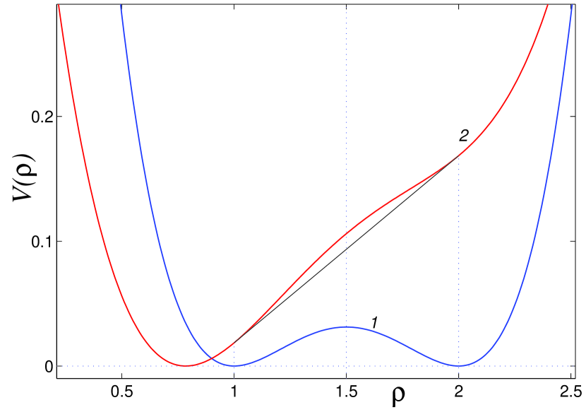
Figure 1: Sketch of double-well potential (2) (curve 1) and single-well potential (8). The straight line connecting the the points $(1,V(1))$ and $(2,V(2))$ of graph single-well potential sets its convex hull.

To simulate the heat transfer in the chain, we use the stochastic Langevin thermostat. The chain has in general $N_{+}+N+N_{-}$ particles. We connect $N_{+}$ particles from one side of the chain to a ”hot” Langevin thermostat with temperature $T_{+}$, and $N_{-}$ particles from the other side – to the Langevin thermostat with temperature $T_{-}$. The corresponding system of equations of motion of the chain can be written as:

$$\ddot{u}_{n} = -\partial H/\partial u_{n}-\gamma\dot{u}_{n}+\xi_{n}^{+},~{}~{}n\leq N_{+},$$

$$\ddot{u}_{n} = -\partial H/\partial u_{n},~{}~{}n=N_{+}+1,...,N_{+}+N,$$ (3)

$$\ddot{u}_{n} = -\partial H/\partial u_{n}-\gamma\dot{u}_{n}+\xi_{n}^{-},~{}~{}n>N_{+}+N,$$

where $\gamma=0.1$ is a relaxation coefficient, $\xi_{n}^{\pm}$ models a white Gaussian noise normalized by the conditions $\langle\xi_{n}^{\pm}(t)\rangle=0$, $\langle\xi_{n}^{+}(t_{1})\xi^{-}_{k}(t_{2})\rangle=0$, $\langle\xi_{n}^{\pm}(t_{1})\xi_{k}^{\pm}(t_{2})\rangle=2\gamma T_{\pm}\delta_{nk}\delta(t_{2}-t_{1})$.

The system of equations of motion (3) was integrated numerically. Considered a chain with fixed ends: $u_{1}\equiv 0$, $u_{N}\equiv(N-1)a$. Used on-initial condition

$$\{u_{n}(0)=(n-1)a,~{}\dot{u}_{n}(0)=0\}_{n=1}^{N},$$

where $1<a<2$ – average value of the chain link length. After an initial transient, thermal equilibrium with the thermostats was established and a stationary heat flux along the chain appeared. A local temperature is numerically defined as $T_{n}=\langle\dot{u}_{n}^{2}\rangle_{t}$ and the local heat flux – as $J_{n}=\bar{a}\langle j_{n}\rangle_{t}$, where $j_{n}=-\dot{u}_{n}V^{\prime}(u_{n}-u_{n-1})$. In numerical simulations we used the following values of temperature $T_{\pm}=(1\pm 0.1)T$ ($T=0.01$, 0.03, 0.1), the relaxation coefficient $\gamma=0.1$, the number of units $N_{\pm}=40$, $N=20$, 40, 80, …, 10240.

This method of thermalization overcomes the problem of the thermal boundary resistance. The distribution of the heat flow $J_{n}$ and the temperature in the chain $T_{n}$ (Fig. 2) clearly demonstrates that inside the ”internal” fragment of the chain $N_{+}<n\leq N_{+}+N$ we observe a heat flux independent on the chain cite, as one would expect in an energy-conserving system. Temperature profile also is almost linear. Thus, from this such simulation one can unambiguously define the heat conduction coefficient of the internal chain fragment:

$$\kappa(N)=J(N-1)/(T_{N_{+}+1}-T_{N_{+}+N}).$$ (4)

Figure 2: Profile of (a) local heat flux $J_{n}$ and (b) local temperature $T_{n}$ in the chain with DW potential (2) for $N_{\pm}=40$, $N=80$, $T_{+}=0.11$, $T_{-}=0.09$. Linear approximation of the temperature distribution (thin red line) is used for evaluation of the heat conduction coefficient $\kappa(N)$.

In thermodynamical limit, one can say that the system obeys the Fourier law, if there exists a finite limit

$$\bar{\kappa}=\lim_{N\rightarrow\infty}\kappa(N).$$

If such limit does exist, one can say that the chain has normal (finite) or convergent heat conduction. In the opposite case, an anomalous heat conduction is observed.

Alternative way for evaluation of the heat conduction coefficient is based on linear response theory, which leads, in particular, to famous Green-Kubo expression GK :

$$\kappa_{c}=\lim_{t\rightarrow\infty}\lim_{N\rightarrow\infty}\frac{1}{NT^{2}}\int_{0}^{t}c(\tau)d\tau,$$ (5)

where the autocorrelation function of the heat flux in the chain is defined as $c(t)=\langle J_{s}(\tau)J_{s}(\tau-t)\rangle_{\tau}$. Here a total heat flux in the chain is defined as $J_{s}(t)=\sum_{n}j_{n}(t)$.

In order to compute the self-correlation function $c(t)$ we simulate a cyclic chain consisting of $N=10^{4}$ particles and couple all these particles to the Langevin thermostat with temperature $T$. After initial thermalization, the chain has been detached from the thermostat and Hamiltonian dynamics has been simulated. In order to improve the accuracy, the self-correlation function has been computed by averaging over $10^{4}$ realizations with independent initial conditions, corresponding to the same initial temperature $T$.

The heat conduction turns out to be convergent if the self-correlation function $c(\tau)$ decreases fast enough as $\tau\rightarrow\infty$. Namely, if the integral in expression (5) converges then the heat conduction may be treated as normal.

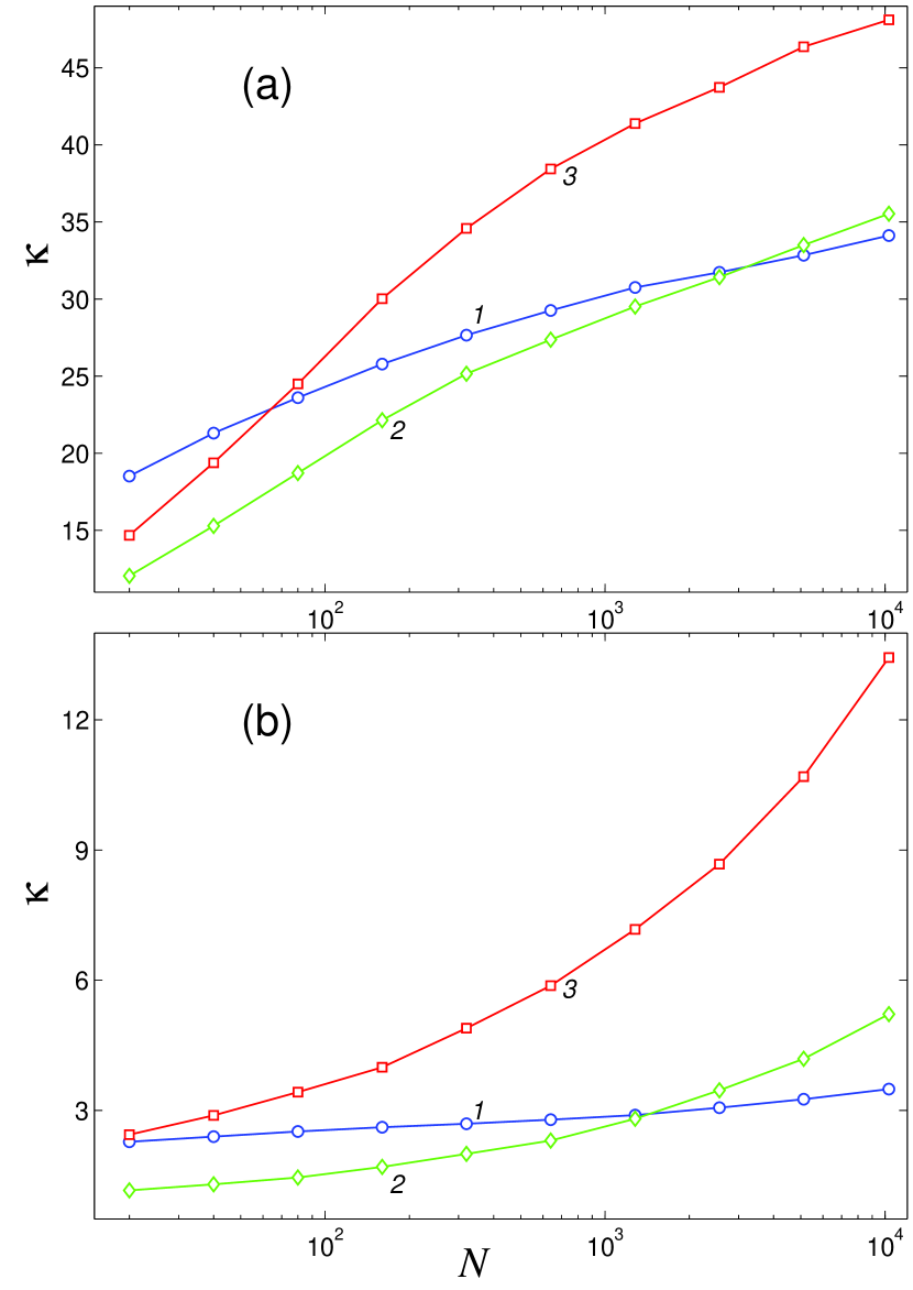
Figure 3: Dependence of the heat conduction coefficient $\kappa$ on the size of the internal chain fragment $N$ for the chain with the DW potential (2) for the average interatomic distance (a) $a=1$ and (b) $a=1.5$ for temperatures $T=0.01$, 0.03, 0.1 (curves 1, 2, 3 respectively).

III Chain with symmetric DW potential

Dependence of the heat conduction coefficient $\kappa$ on the length of the chain fragment between the Langevin thermostats $N$ for the chain with symmetric DW potential (2) is presented in Fig. 3. As one can see from this figure, both for $a=1$ and $a=1.5$ the heat conduction coefficient gown monotonously with $N$ and demonstrates no trend for convergence. For $a=1.5$ the heat conduction coefficient grows like $N^{\alpha}$, with $\alpha=0.09$ for the temperature $T=0.01$ and $\alpha=0.29$ for $T=0.03$, 0.1, as it is demonstrated in Fig. 4.

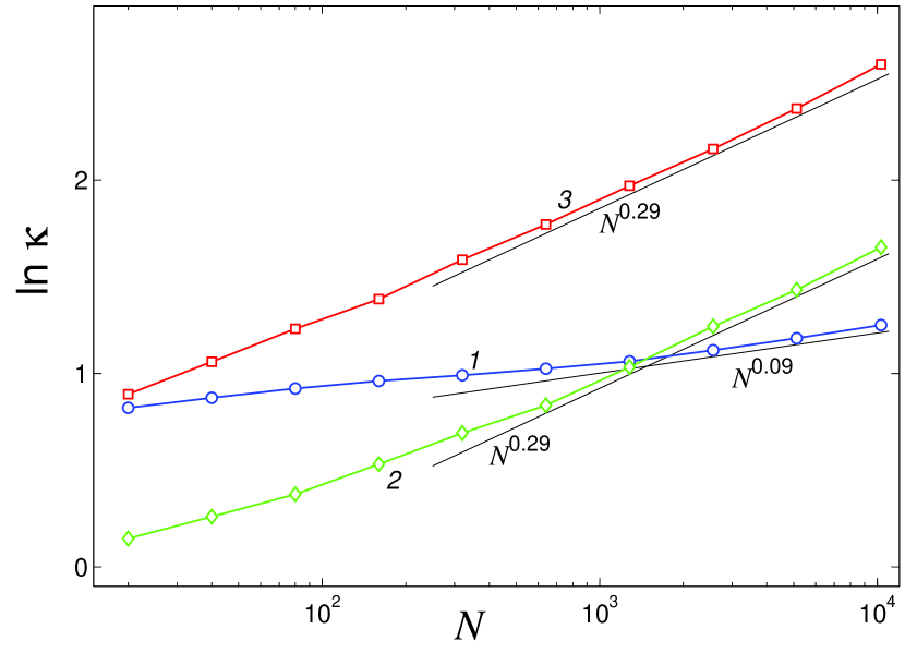
Figure 4: Dependence of the heat conduction coefficient $\kappa$ on the size of the internal chain fragment $N$ for the chain with the DW potential (2) for the average interatomic distance $a=1.5$ for temperatures $T=0.01$, 0.03, 0.1 (curves 1, 2, 3 respectively). The graphs are presented in double logarithmic scale and straight lines correspond to fitting $N^{\alpha}$, $\alpha=0.09,0.29,0.29$ for curves 1, 2, 3 respectively.

Numeric analysis of the heat flux autocorrelation function $c(t)$ as $t\rightarrow\infty$ supports the conclusion on divergent heat conductivity in the system. For all values of the average link length $1\leq a\leq 2$ the function $c(t)$ decreases as $t\rightarrow\infty$ according to the power law $t^{-\beta}$ with exponent $\beta<1$, as it is demonstrated in Fig. 5. According to Green-Kubo formula (5) one arrives to the same conclusion on divergence of the heat conduction coefficient $\kappa(N)$ as $N\rightarrow\infty$. Two approaches used here are independent and point in the same direction – one obtains clear indication that the heat conductivity in the chain with DW potential diverges.

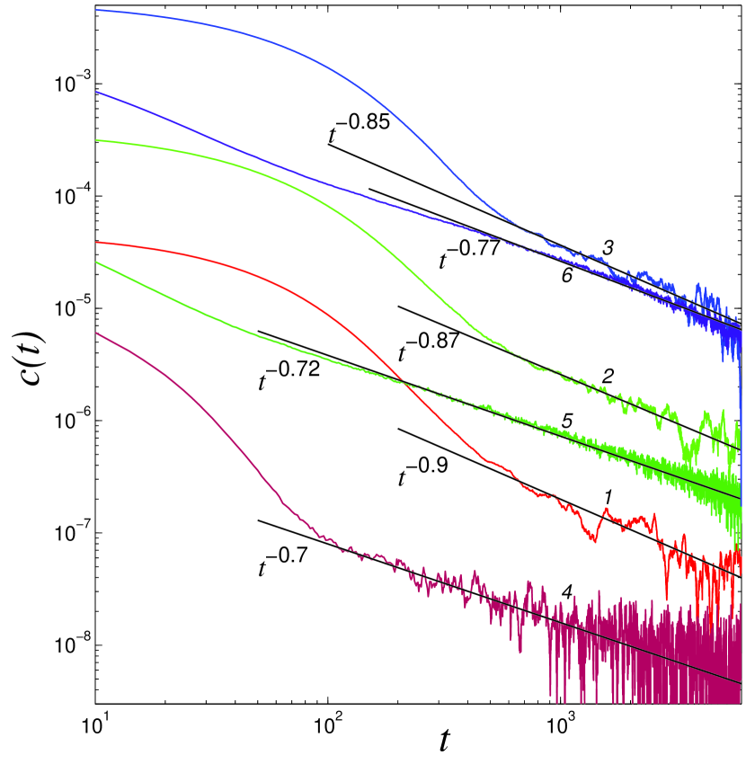
Figure 5: Power-law decrease of the autocorrelation function $c(t)$ for the chain with symmetric DW potential (2) for average link length $a=1$ and temperatures $T=0.01$, 0.03, 0.1 (curves 1, 2, 3 respectively) and $a=1.5$, $T=0.01$, 0.03, 0.1 (curves 4, 5, 6 respectively). The graphs are presented in double logarithmic scale and straight lines correspond to fitting $t^{-\beta}$, $\beta=0.9,0.87,0.85,0.7,0.72,0.77$ for curves 1, 2,…, 6 respectively.

So, as it was already mentioned in the Introduction, it is reasonable to explore and compare the heat conduction coefficient $\kappa(N)$ for some fixed chain length. To be specific, we choose $N=640$ and consider the temperature dependence of the heat conductivity for fixed number of particles and varying average link length. The results are presented in Fig. 6. For all presented values of the link length the heat conductivity in the case of low temperatures $T<0.01$ sharply decreases as the temperature grows. For large temperatures the heat conductivity weakly increases with the temperature. In all cases the minimum is achieved in the temperature interval $0.01\div 0.04$, which is close to the height of the potential barrier. The lowest values of the heat conduction coefficient are obtained for $a=1.5$. This result is quite expectable, since namely for this value of the average link length the number of topologically different degenerate ground states achieves a maximum.

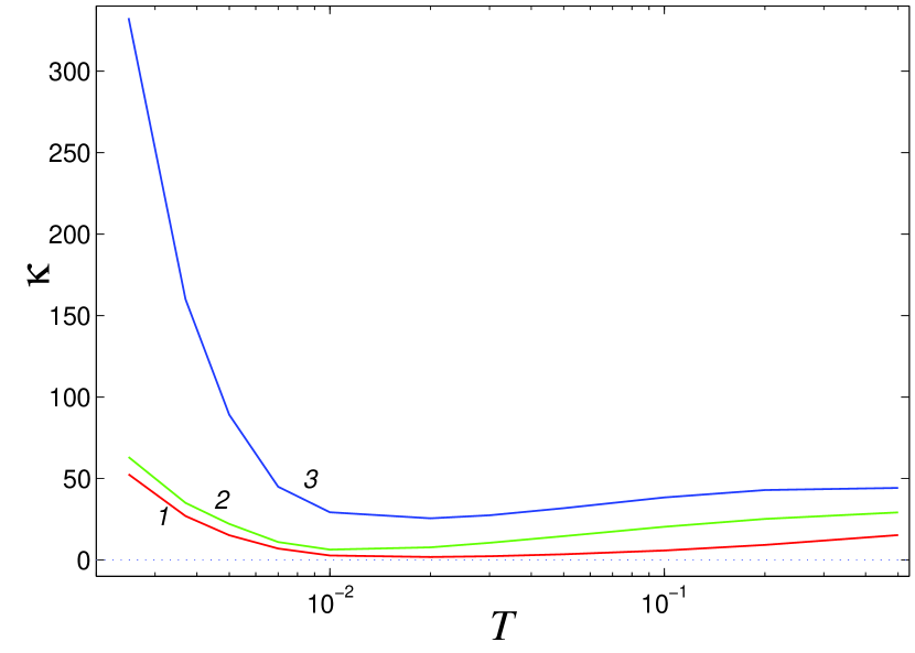
Figure 6: Dependence of the heat conduction coefficient $\kappa$ on temperature $T$ of the chain containing in general $720$ particles ($N=640$, $N_{\pm}=40$) with the DW potential (2) for $a=1.5$, 1.1, 1.0 (curves 1, 2, 3 respectively).

From Fig. 6 one can see that if the average link length $a$ varies from 1 to 1.5, the heat conduction coefficient decreases monotonously. In order to estimate the efficiency of the heat conductivity reduction, we define the reduction coefficient $\mu_{a}=\kappa(a,N,T)/\kappa(1,N,T)$, where $\kappa(a,N,T)$ denotes the heat conduction coefficient for the average link length $a$, number of particles $N$ and temperature $T$. We note that by symmetry considerations it is enough to consider only the interval $1\leq a\leq 1.5$.

A dependence of $\mu_{a}$ on the temperature and the average link length is presented in Fig. 7. The heat conductivity decreases with increase of $a$ for all studied values of the temperature. Maximal efficiency of the reduction is achieved for the temperature $T=0.02$, which is close to the height of the potential barrier $E_{0}=0.0313$. As one could expect, maximal reduction of the heat conductivity occurs at $a=1.5$.

However, other aspect of the reduction phenomenon is somewhat unexpected. In Fig. 8 we present the dependence of the reduction efficiency for different temperatures $\mu_{N}=\kappa(1.5,N,T)/\kappa(1,N,T)$ as a function of the particle number $N$. It is somewhat surprising to see that this dependence is not monotonous. The chain length for which the most efficient reduction of the heat conductivity is observed, strongly depends on the temperature. For instance, for $T=0.01$ the most efficient reduction is observed when $N_{0}=1280$, and for higher temperatures $T=0.03,0.1$ – when $N_{0}=160$.

It is easy to explain why for relatively short chains the reduction efficiency is higher when the chain gets longer. We believe that the reduction of the heat conductivity occurs due to increase of a number of the degenerate ground states. Quite obviously, this effect becomes more profound as the number of particles grows. The decrease of the reduction efficiency for relatively high $N$ is more difficult to explain. Qualitatively, one can speculate that, since the heat conduction coefficient in the chain with DW potential diverges, for very large $N$ the heat transfer is governed by long-wavelength weakly interacting phonons. Such waves are less sensitive to the details of the chain structure and ”feel”  only average density of the particles.

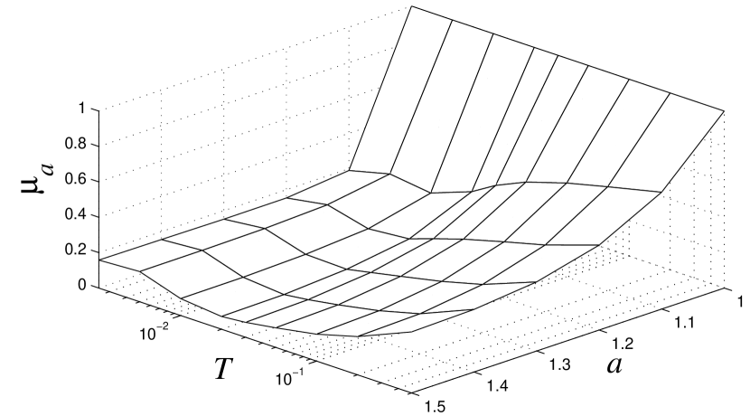
Figure 7: Temperature dependence of the reduction coefficient $\mu_{a}=\kappa(a)/\kappa(1)$ on the average link length $a$.

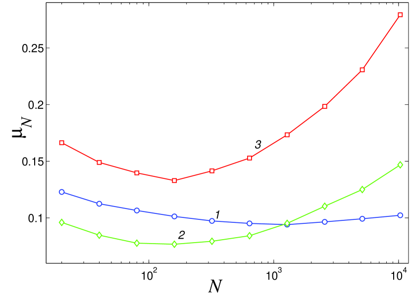
Figure 8: Dependence of the reduction coefficient $\mu_{N}=\kappa(1.5)/\kappa(1)$ on the chain length $N$ for temperature values $T=0.01,0.03,0.1$ (curves 1, 2, 3 respectively).

It is also instructive to compare the process of non-stationary heat conduction in the DW model with different average link length. For this sake, following a methodology developed in GSNS1 ; GSNS2 , we simulate a relaxation of various spatial modes of a thermal perturbation in the cyclic DW chain with $N$ particles. Thus, the initial temperature distribution is defined according to the following relationship:

$$T_{n}=T_{0}+A\cos[2\pi(n-1)/Z],$$ (6)

where $T_{0}$ is the average temperature, $A$ is the amplitude of the perturbation, and $Z$ is the length of the mode (number of particles). The overall number of particles $N$ has to be multiple of $Z$ in order to ensure the periodic boundary conditions.

In order to realize this initial thermal perturbation, each particle in the chain is first attached to a separate Langevin thermostat. In other terms, we integrate numerically the following system of equations:

$$\ddot{u}_{n}=-\partial H/\partial u_{n}-\gamma\dot{u}_{n}+\xi_{n},$$ (7)

where $n=1,2,...,N$, $\gamma=0.1$, and the action of the thermostat is simulated as white Gaussian noise normalized according to conditions

$$\langle\xi_{n}(t_{1})\xi_{k}(t_{2})\rangle=2\gamma T_{n}\delta_{kn}\delta(t_{2}-t_{1}).$$

After the initial heating in accordance with (6), the Langevin thermostat is removed and relaxation of the system to a stationary temperature profile is studied. The results were averaged over $10^{6}$ realizations of the initial profile $\{T_{n}\}_{n=1}^{N}$ in order to reduce the effect of fluctuations.

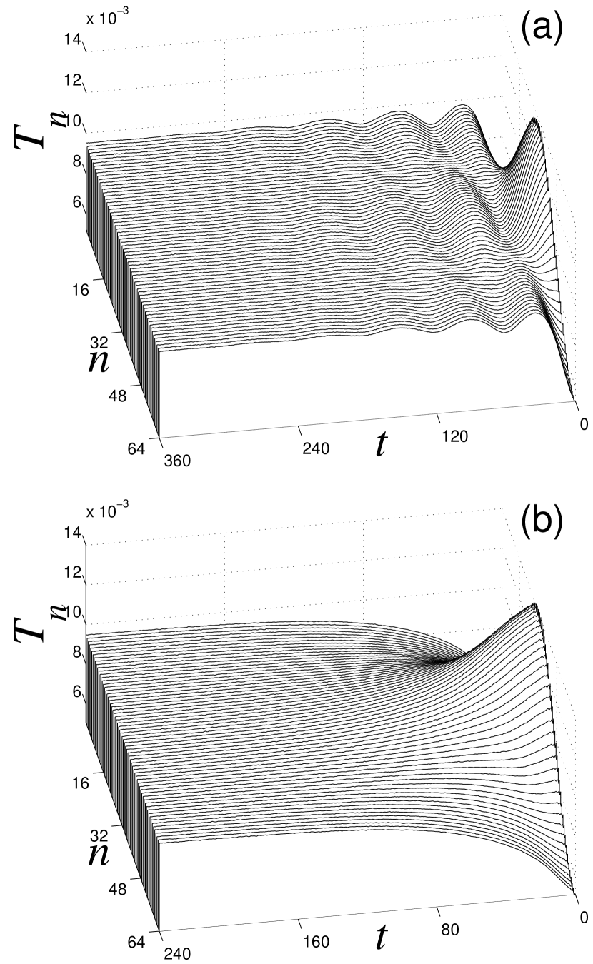
Figure 9: Relaxation of initial periodic thermal profile in the periodic chain with potential (2) $N=1024$, $T_{0}=0.01$, $A=0.05$, $Z=64$ for (a) $a=1$ and (b) $a=1.5$.

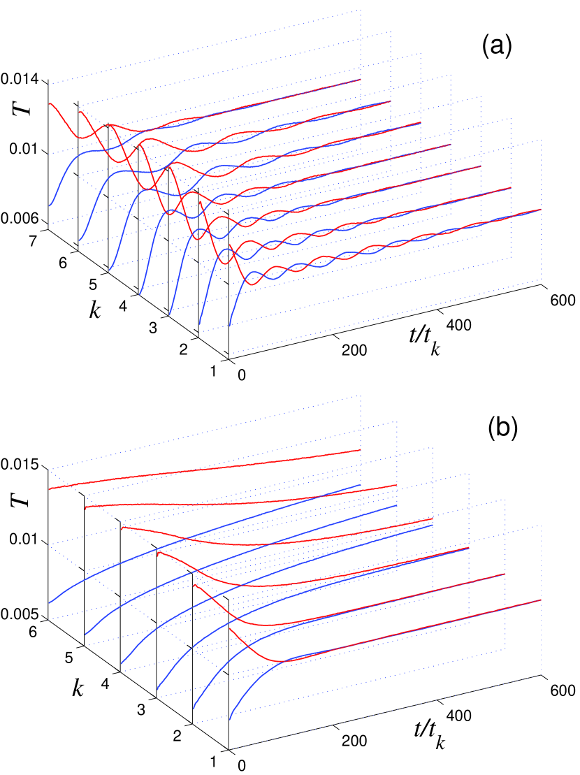
Figure 10: Evolution of the relaxation profile in the periodic chain with double-well potential (2) ($N=2048$, $T_{0}=0.01$, $A=0.05$) for (a) $a=1$ ($Z=2^{3+k}$, $k=1,2,...,7$, $t_{k}=0.15$, 0.3, 0.6, 1.2, 2.0, 4.0, 10.0) and (b) $a=1.5$ ($Z=2^{3+k}$, $t_{k}=0.1\cdot 2^{k-1}$, $k=1,2,...,6$). Time dependence of the mode maximum $T(1+Z/2)$ [red (gray) lines] and minimum T(1) [blue (black) lines] are depicted.

Samples of the non-stationary simulations are presented in Figs. 9 and 10. In both figures, we compare the relaxation of similar thermal perturbation profiles with similar average temperature, perturbation amplitude and spatial wavelength. The only difference is the average link length. We compare the two extreme cases $a=1$ and $a=1.5$. In Fig. 10 one can see that the same thermal perturbation for $a=1$ decays in oscillatory manner, whereas for $a=1.5$ the decay is smooth. Thus, one can suggest that for the case $a=1$ one should take into account phenomena related to hyperbolic corrections to Fourier law (like possibility of the second sound); in the same time, for the case $a=1.5$ one should expect primarily diffusive behavior. This conclusion is further confirmed by simulation results presented in Fig. 9. There we can see that for $a=1$ the oscillatory (i.e. hyperbolic) behavior is observed for very broad diapason of the wavelengths. For all these modes, the thermal perturbations for $a=1.5$ decay in primarily diffusive manner. The reason for this difference, again, is a ”perfect” structure of the ground state for $a=1$ and large number of the degenerate ground states for $a=1.5$.

IV A model with non-convex single-well potential

The results presented in the previous Section suggest that the increase of the number of the ground states peculiar for the DW chain leads to suppression of the heat conduction. One should expect even stronger suppression effect, when the chain is modified in a way that the potential changes from single-well to double-well. Possibility of such modification in particular chain model under action of an external force, and the consequences for the heat conductivity are discussed here. First of all, we suggest a model of the chain with a non-convex single well potential of the nearest-neighbor interaction:

$$V(\rho)=\epsilon(\rho-1)^{2}(\rho-2)^{2}+\beta\rho+c,$$ (8)

where $\epsilon=1/2$, $\beta=0.15$, and (physically insignificant) constant $c$ may be found from a condition $\min V(\rho)=0$. Under these values of parameters potential function (8) has a single minimum at $\rho_{0}=0.89$ (Fig. 1).

Let us consider the case when the chain with potential (8) is elongated by external force $F$ applied to one of its ends, whereas the other end remains fixed. It is easy to see that such external forcing is equivalent to a modification of the interaction potential (8) by addition of negative linear term. This modified potential will have the following form:

$$V^{*}(\rho)=\epsilon(\rho-1)^{2}(\rho-2)^{2}+\beta\rho-F\rho+c.$$ (9)

Thus, the application of the external force can modify the qualitative shape of the potential function. Namely, it is easy to demonstrate that for $F<F_{min}=\beta-\epsilon/3\sqrt{3}$ and for $F>F_{max}=\beta+\epsilon/3\sqrt{3}$ the potential $V^{*}(\rho)$ remains single-well. However for $F_{min}<F<F_{max}$ the effective potential becomes double-well and thus one can expect significant reduction of the heat conductivity as a result of application of the external force.

In our numeric experiments we control the average link length $a$ rather than the value of the external force. However, it is easy to translate between these quantities. Namely, potential function (9) will have two wells if the following condition holds: $a_{min}<a<a_{max}$, where $a_{min}=3/2-1/\sqrt{3}\approx 0.9226$ and $a_{max}=3/2+1/\sqrt{3}\approx 2.0774$.

Creation of the effective double-well potential can be also explained from observation of the single-well potential function (8) depicted in Fig. 1. One can see that this function is not convex (the second derivative is negative for $1\leq\rho\leq 2$). Homogeneous extension of such chain, when all the links have the same length $\rho_{n}\equiv a>\rho_{0}$, is energetically favorable only when the average link length belongs to the interval where the potential function has positive second derivative: $a\leq\rho_{1}=1$ and $a\geq\rho_{2}=2$. If $\rho_{1}<a<\rho_{2}$, it is more favorable to have part of the links with the length $\rho_{n}\equiv\rho_{1}=1$, and the rest of the links – with the length $\rho_{n}\equiv\rho_{2}=2$. In this case, the dependence of the average potential energy per particle on the average link length will follow the straight line connecting the points $(\rho_{1},V(\rho_{1}))$ and $(\rho_{2},V(\rho_{2}))$, as it is demonstrated in Fig. 1 Savin_pnas ; smko13 . Thus, as the average link length increases, the numbers of ”short” and ”long” links vary accordingly, thus giving rise to large number of possible realizations and large variations of the heat conduction coefficient.

Heat transfer in this system has been simulated with the help of Langevin thermostats (3) under fixed-ends boundary conditions: $u_{1}(t)\equiv 0$, $u_{N_{+}+N+N_{-}}=(N_{+}+N+N_{-}-1)a$, where again $a\geq\rho_{0}$ is the average length of the link.

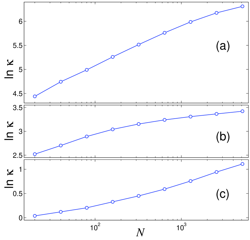
Figure 11: Dependence of heat conduction coefficient $\kappa$ on the chain length $N$ for the chain with single-well nearest-neighbor potential (8) for different values of the average link length: (a) $a=\rho_{0}$, (b) $a=2.0$, (c) $a=1.5$. In all cases the temperature $T=0.01$.

Numeric simulation of the heat conduction demonstrated that for all studied values of the average link length $a\geq\rho_{0}$ the heat conduction coefficient diverges: $\kappa(N)\nearrow\infty$ as $N\nearrow\infty$ – see. Fig. 11. Equilibrium simulations based on Green-Kubo formula (5) bring about the same conclusion.

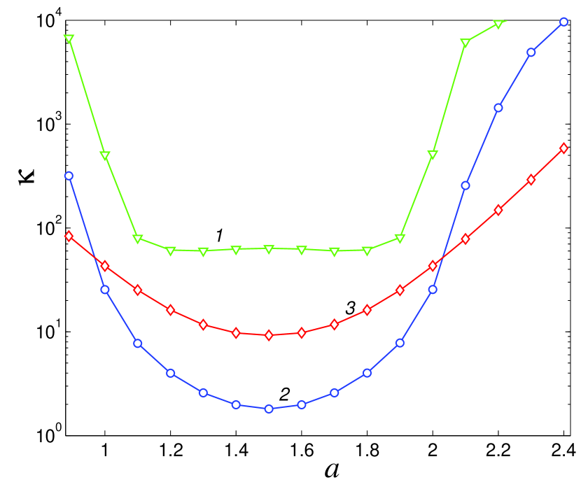
Figure 12: Dependence of the heat conduction coefficient $\kappa$ in the chain with single-well potential of the nearest-neighbor interaction (8) on the average link length $a$ for temperatures $T=0.002$, 0.02, 0.2 (curves 1, 2, 3 respectively). Note a logarithmic scale for $\kappa$. Simulated chain contained in all cases $N_{+}+N+N_{-}$ particles, $N=640$ of them were free and $N_{\pm}=40$ were immersed in the Langevin thermostats with temperatures $T_{\pm}=(1\pm 0.1)T$.

The dependence of the heat conduction coefficient $\kappa$ on the average link length $a$ for the chain with the single-well non-convex potential of the nearest-neighbor interaction (8) is presented in Fig. 12. One can observe extremely significant effect of the chain extension on the heat conduction coefficient. This drastic reduction is observed for values of the average link length approximately in the interval $1<a<2$, in accordance with earlier findings on relationship between a number of possible degenerate (or close energetically) ground states and the reduction of the heat conductivity.

It is possible to say that these drastic modifications of the heat conduction coefficient occur due to ”latent” double-well nature of the non-convex potential of the nearest-neighbor interaction. Notably, the most efficient reduction is achieved when the temperature is close to the height $\epsilon$ of the ”latent” potential barrier. The reduction of the heat conductivity by two orders of magnitude is achieved for $T=0.02$.

It is important to mention that the effective non-convex single-well potential is obtained in effective models of some quasi-one-dimensional objects. For instance, it is realized in $\alpha$-spirals of protein macromolecules, double helix of DNA Savin_pnas ; smko13 , as well as in a model of intermetallic NiAl crystalline nanofilms Dmitriev . In these structures the external extension brings a non-homogeneous equilibrium configurations. Then, one should expect strong effect of external mechanic loads on transport properties in systems of this sort.

V Control in models with convergent heat conduction

All simple models considered above are commonly believed to have the divergent heat conductivity in the thermodynamical limit. In this section, we are going to consider a modification of chain of rotators, which allows external control of the heat conduction coefficient. Simple chain of rotators is believed to exhibit convergent heat conductivity giardina ; savin2 .

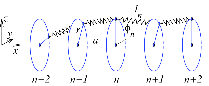
Figure 13: Sketch of the modified chain of rotators

To explain the idea of possible modification, let us consider a mechanical model sketched in Fig. 13 – a chain of equal parallel disks of radius $r$ with centers fixed at equal intervals of length $a$ along $x$ axis. The disks can rotate along $x$ axis and the rotation angle of the $n$-th disk is denoted as $\phi_{n}$. Neighboring disks are coupled by harmonic springs of equal stiffness and equilibrium length. Hamiltonian of such model can be simply expressed as follows:

$$H=\sum_{n=1}^{N}\frac{1}{2}I\dot{\phi}_{n}^{2}+V(\phi_{n+1}-\phi_{n}),$$ (10)

where $I$ is a moment of inertia of the disk. Potential energy of relative rotation appears due to deformation of the springs, which couple the neighboring disks, and is expressed as

$$V(\Delta\phi_{n})=\frac{1}{2}K(l_{n}-L_{0})^{2}$$

$$=\frac{1}{2}K\{[a^{2}+2r^{2}(1-\cos(\Delta\phi_{n})]^{1/2}-L_{0}\}^{2},$$ (11)

Here $\Delta\phi_{n}=\phi_{n+1}-\phi_{n}$ is a relative rotation angle of the neighboring disks, $K$ and $L_{0}$ are the stiffness and equilibrium length of the springs respectively, $l_{n}$ is the length of the $n$-th spring. Potential function (11) will be double-well provided that $a<L_{0}<[a^{2}+4r^{2}]^{1/2}$. The potential minima in this case correspond to the following values of the relative rotation angle:

$$\Delta\phi_{0}=\pm 2\arcsin\{[(L_{0}^{2}-a^{2})/4r^{2}]^{1/2}\}.$$

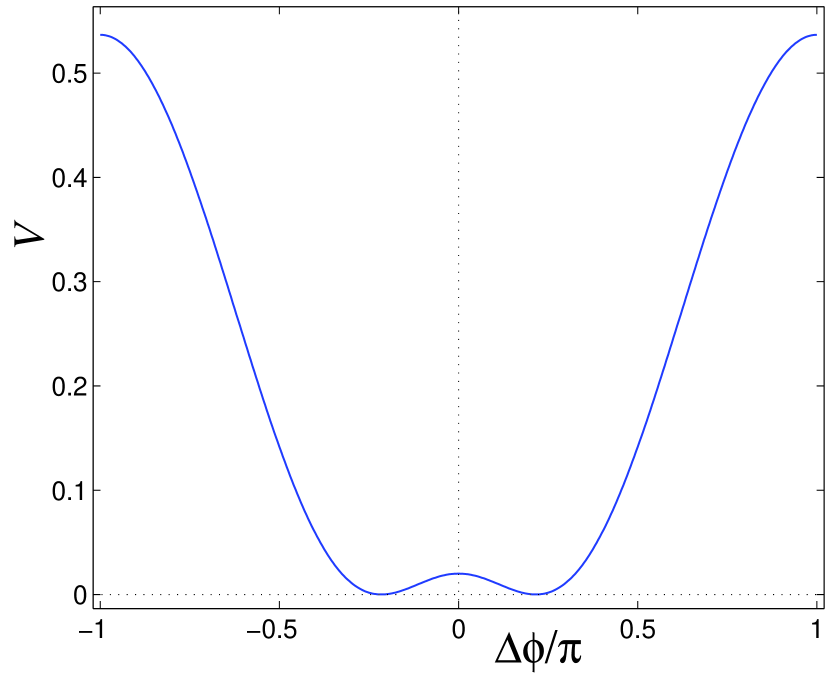
Figure 14: Shape of potential function (11) $V(\Delta\phi)$ for $a=1$, $r=1$, $L_{0}=1.2$, $K=1$. Heights of the potential barriers are $\epsilon_{0}=0.02$, $\epsilon_{1}=0.5367$. The potential function achieves the minima for $\Delta\phi=\pm 0.2152\pi$.

Characteristic shape of the modified potential function (11) is presented in Fig. 14. Without affecting the generality, one can set $I=1$, $a=1$ and $K=1$. To be specific, we also choose $r=1$. Thus, the potential will have two wells for the equilibrium length of the spring in the interval $1<L_{0}<\sqrt{5}$. The function $V(\Delta\phi)$ is $2\pi$-periodic and has two potential barriers $0<\epsilon_{0}<\epsilon_{1}$. If the equilibrium spring length $L_{0}$ will only slightly exceed the distance $a$ between the disk centers, then one will obtain $\epsilon_{0}\ll\epsilon_{1}$. For instance, for $L_{0}=1.2$ one obtains the potential minima $\Delta\phi_{0}=\pm 0.2152\pi\approx 0.6761$, and the barriers $\epsilon_{0}=0.02$, $\epsilon_{1}=0.5367$.

We expect that, similarly to the simple chain of dipole rotators giardina ; savin2 , the chain with Hamiltonian (10) will have converging heat conduction coefficient.

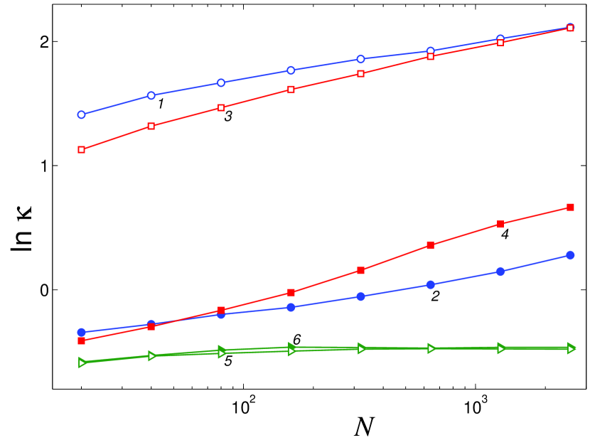
Figure 15: Dependence of the heat conduction coefficient $\kappa$ on the size of the internal chain fragment $N$ for the chain with periodic potential (11) for the average angle between the disks $\varphi_{0}=\Delta\phi_{0}$ and $\varphi_{0}=0$ respectively (curves 1 and 2 for temperature $T$=0.01, curves 3 and 4 – for $T=0.02$, curves 5 and 6 – for $T=0.2$).

To simulate the heat conductivity, we attach the chain ends with $N_{\pm}=40$ disks to Langevin thermostats with temperatures $T_{\pm}=(1\pm 0.1)T$. Then, we simulate numerically the system of equation (3) with potential function obtained from (11) under fixed boundary conditions $\varphi_{0}\equiv 0$, $\varphi_{M}\equiv(N_{+}+N+N_{-}-1)\varphi_{0}$ and with initial conditions

$$\{\varphi_{n}(0)=(n-1)\varphi_{0},~{}~{}\dot{\varphi}_{n}(0)=0\}_{n=1}^{N_{+}+N+N_{-}},$$

where $\varphi_{0}$ – average value of angle between neighboring disks. In other terms, we keep constant relative rotation angle between the ends of the chain (in other terms, we apply constant momentum to the chain) and study the dependence of the heat conduction coefficient on these external conditions.

Dependence of the heat conduction coefficient $\kappa$ on the length of the chain fragment between the Langevin thermostats $N$ for the chain with periodic potential (11) is presented in Fig. 15. As one can see, the value of $N$ for which the heat conductivity converges, strongly depends on the average temperature $T$.

For average temperature $T=0.2$ comparable to a value of the higher potential barrier $\epsilon_{1}$, the convergence is reliably achieved already for $N=320$. We also see that the heat conduction coefficient almost does not depend on $\varphi_{0}$. The latter result seems natural, since the temperature is large enough to allow frequent transitions over the higher barrier; then, the initial mutual rotation of the disks is relaxed.

If the average temperature will be much lower than the higher potential barrier $T\ll\epsilon_{1}$, the relaxation mentioned above will require exponentially large time. In this case, the heat conduction still converges, but the convergence requires consideration of essentially larger values of the chain length $N$. For every chain length, the heat conductivity in the chains with $\varphi_{0}=0$ is significantly higher that in the chains with $\varphi_{0}=\Delta\phi_{0}$. For the average temperature $T=0.01$ the difference is 6.5 times, and for $T=0.02$ – 5 times.

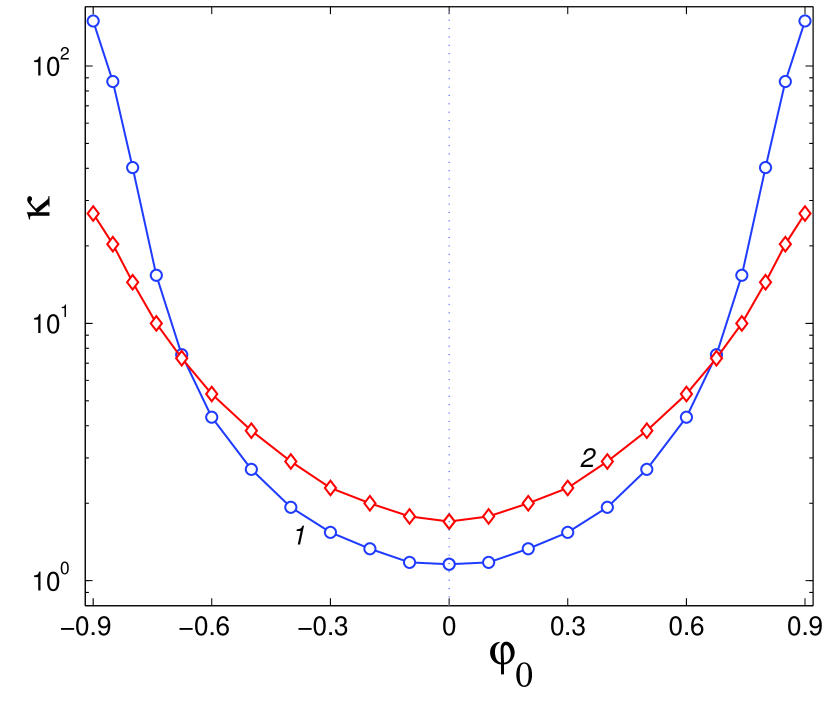
Figure 16: (a) Dependence of the heat conduction coefficient $\kappa$ in the chain with periodic potential of the nearest-neighbor interaction (11) on the average interdipole angle $\varphi_{0}$ for temperatures $T=0.01$, 0.02 (curves 1, 2 respectively).

To check this assumption further, let us consider also the dependence of $\kappa$ on the initial angle between the disks $\varphi_{0}$ for the chain length $N=1280$. In Fig. 16, one can clearly observe that this dependence is strong enough, provided that the temperature is sufficiently low to prevent the fast relaxation.

Physical reasons of this behavior are very similar to those described in the preceding Sections. For $|\varphi_{0}|\leq\Delta\phi_{0}$ the chain has energetically degenerate ground states, where part of the neighboring disk pairs have relative equilibrium angle $\phi_{n+1}-\phi_{n}=\Delta\phi_{0}$, and the other pairs – $\phi_{n+1}-\phi_{n}=-\Delta\phi_{0}$. A number of possible different ground states grows as $|\varphi_{0}|$ tends to zero. That is why the heat conductivity decreases in this limit. This effect becomes more pronounced as the temperature decreases. Still, for extremely small temperatures the heat conductivity will cease to depend on $|\varphi_{0}|$, since even the smaller potential barriers will become prohibitive.

For exponentially large simulation times the dependence of the heat conductivity on the initial relative rotation of the disks is expected to disappear due to thermally activated relaxation over higher potential barriers. In our simulations the times were not large enough to observe this relaxation for lower temperatures. Still, we believe that this problem may be easily overcome. It seems sufficient to act with constant external momentum on the right end of the chain, rather than to fix it. Then, one should investigate a dependence of the heat conduction coefficient on the value of this external momentum.

The idea presented in this Section could be useful for practical design of the systems with controlled heat conductivity. One can use, for instance, the stretched polymer macromolecules. Their heat conductivity can be modified by application of the external momentum.

Concluding remarks

In this paper we demonstrated that one can efficiently control the transport properties of model atomic chains by purely mechanical means. In the case of the chain with double-well interparticle potential, it is enough to change the average interparticle distance in order to modify a number of possible degenerate ground states and to reduce or to increase the heat conductivity. The effect is rather pronounced (about five-fold reduction was observed). However, even stronger effect – reduction by two orders of magnitude – was observed in more realistic model with single-well nonconvex interparticle potential. In this model the heat conductivity is directly related to applied external strain. Also in this case it seems that the reduction effect is caused by formation of ”effective” double-well potential and variation of a number of possible states of mechanical equilibrium.

Modification of thermal conductivity in conditions of external mechanical load can be related to broader field of thermoelasticity. It is well-known that elasticity and plasticity in real materials can be strongly coupled with thermodynamic phenomena and heat transport. It seems, however, that this possible coupling has not received proper attention in numerous recent studies devoted to microscopic foundations of the heat conductivity. Our results demonstrate that these effects can be rather profound. One can be tempted to say that the extension of the chain with the DW potential exemplifies the effect of plasticity on the heat transport. The chain with the single-well potential requires constant external forcing to reduce the heat conductivity; this phenomenon is primarily elastic. Needless to say, these statements are quite crude and schematic; still we believe that the subject is of considerable fundamental interest. Besides, interesting practical implications are straightforward – one can be interested in simple mechanical means of control over heat transport in micro- and nanosystems.

References

- (1) S. Lepri, R. Livi, A. Politi. Thermal conduction in classical low-dimensional lattices. Physics Reports 377, 1-80 (2003).
- (2) E. Fermi, J. Pasta, S. Ulam. Studies of non linear problems. Los Alamos Rpt LA.1940 (1955).
- (3) S. Lepri, L. Roberto, A. Politi. Heat Conduction in Chains of Nonlinear Oscillators. Phys. Rev. Lett. 78, 1896 (1997).
- (4) S. Lepri, R. Livi, A. Politi. Energy transport in anharmonic lattices close and far from equilibrium. Physica D 119, 140 (1998).
- (5) S. Lepri, R. Livi, A. Politi. On the anomalous thermal conductivity of one-dimensional lattices. Evrophys. Lett. 43, 271 (1998).
- (6) R. Rubin and W. Greer, Abnormal Lattice Thermal Conductivity of a One-Dimensional, Harmonic, Isotopically Disordered Crystal. J. Math. Phys. 12, 1686 (1971).
- (7) A. Casher and J.L. Lebowitz, Heat Flow in Regular and Disordered Harmonic Chains. J. Math. Phys. 12, 1701 (1971).
- (8) A. Dhar, Heat Conduction in the Disordered Harmonic Chain Revisited. Phys. Rev. Lett. 86, 5882 (2001).
- (9) A. Dhar, Heat Conduction in a One-Dimensional Gas of Elastically Colliding Particles of Unequal Masses. Phys. Rev. Lett. 86, 3554 (2001).
- (10) A.V. Savin, G.P. Tsironis, and A.V. Zolotaryuk, Heat Conduction in One-Dimensional Systems with Hard-Point Interparticle Interactions. Phys. Rev. Lett. 88, 154301 (2002).
- (11) P. Grassberger, W. Nadler, and L. Yang, Heat Conduction and Entropy Production in a One-Dimensional Hard-Particle Gas. Phys. Rev. Lett. 89, 180601 (2002).
- (12) T. Hatano. Heat conduction in the diatomic Toda lattice revisited. Phys. Rev. E 59, R1 (1999).
- (13) B. Hu, B. Li, and H. Zhao, Heat conduction in one-dimensional chains. Phys. Rev. E 57, 2992 (1998).
- (14) A. V. Savin and O. V. Gendelman, Heat conduction in one-dimensional lattices with on-site potential. Phys. Rev. E 67, 041205 (2003).
- (15) G.P. Tsironis, A.R. Bishop, A.V. Savin, and A.V. Zolotaryuk, Dependence of thermal conductivity on discrete breathers in lattices. Phys. Rev. E 60, 6610 (1999).
- (16) B. Hu, B. Li, and H. Zhao, Heat conduction in one-dimensional nonintegrable systems. Phys. Rev. E 61, 3828 (2000).
- (17) K. Aoki and D. Kuznezov, Bulk properties of anharmonic chains in strong thermal gradients: non-equilibrium theory. Phys. Lett. A 265, 250 (2000).
- (18) O.V. Gendelman and A.V. Savin. Heat Conduction in a One-Dimensional Chain of Hard Disks with Substrate Potential. Phys. Rev. Lett. 92(7), 074301 (2004).
- (19) C. Giardina, R. Livi, A. Politi, and M. Vassalli. Finite thermal conductivity in 1D lattices. Phys. Rev. Lett. 84, 2144 (2000).
- (20) O. V. Gendelman and A. V. Savin. Normal heat conductivity of the one-dimensional lattice with periodic potential of nearest-neighbor interaction. Phys. Rev. Lett. 84, 2381 (2000).
- (21) Y. Zhong, Y. Zhang, J. Wang and H. Zhao. Normal heat conduction in one-dimensional momentum conserving lattices with asymmetric interactions. Phys. Rev. E 85, 060102(R) (2012).
- (22) S. Chen, Y. Zhang, J. Wang, and H. Zhao. Breakdown of the power-law decay prediction of the heat current correlation in one-dimensional momentum conserving lattices. arXiv:1204.5933v3 [cond-mat.stat-mech] 15 Oct 2012.
- (23) A. V. Savin and Y. A. Kosevich Thermal conductivity of the chain with an asymmetric pair interaction. arXiv:submit/0761690 [cond-mat.stat-mech] 17 Jul 2013.
- (24) R. Kubo, M. Toda, N. Hashitsume. Statistical Physics II. / Springer, Ser. Solid State Sci. V. 31 (1991).
- (25) A. Fillipov, B. Hu, B. Li, and A. Zeltser. Energy transport between two attractors connected by a Fermi-Pasta-Ulam chain. J. Phys. A: Math. Gen. 31, 7719 (1998).
- (26) F. Legoll, M. Luskin, and R. Moeckel. Non-ergodicity of Nose-Hoover dynamics. Nonlinearity 22, 1673 (2009).
- (27) D. Roy. Crossover from Fermi-Pasta-Ulam to normal diffusive behavior in heat conduction through open anharmonic lattices. Phys. Rev. E 86, 041102 (2013).
- (28) O.V.Gendelman and A.V.Savin. Nonstationary heat conduction in one-dimensional chains with conserved momentum Phys Rev. E 81, 011105 (2012)
- (29) O.V.Gendelman, R.Shvartsman, B.Madar and A.V.Savin. Nonstationary heat conduction in one-dimensional models with substrate potential Phys Rev. E 86, 020103(R) (2010)
- (30) A. V. Savin, I. P. Kikot, M. A. Mazo, and A. V. Onufriev. Two-phase stretching of molecular chains. PNAS February 1, 2013 201218677.
- (31) A. V. Savin, M. A. Mazo, I. P. Kikot, A. V. Onufriev Two-phase stretching of molecular chains. arXiv:1110.3165v2 [cond-mat.mes-hall] 25 Feb 2013.
- (32) R. I. Babicheva, K. A. Bukreeva, S. V. Dmitriev, and K. Zhou. Discontinuous elastic strain observed during stretching of NiAl signal crystal nanofilms. Computational Materials Science 80 (2013).