Hubbard-corrected DFT energy functionals: the LDA+U description of correlated systems

Abstract

The aim of this review article is to assess the descriptive capabilities of the Hubbard-rooted LDA+U method and to clarify the conditions under which it can be expected to be most predictive. The paper illustrates the theoretical foundation of LDA+U and prototypical applictions to the study of correlated materials, discusses the most relevant approximations used in its formulation, and makes a comparison with other approaches also developed for similar purposes. Open “issues” of the method are also discussed, including the calculation of the electronic couplings (the Hubbard $U$), the precise expression of the corrective functional and the possibility to use LDA+U for other classes of materials. The second part of the article presents recent extensions to the method and illustrates the significant improvements they have obtained in the description of several classes of different systems. The conclusive section finally discusses possible future developments of LDA+U to further enlarge its predictive power and its range of applicability.

I Introduction

After almost five decades from its formulation hohenberg64 ; kohn65 , Density Functional Theory (DFT) still represents the main computational tool to perform electronic structure calculations for systems of realistic complexity. The possibility to express all the ground state properties of a system as functionals of its electronic charge density and the existence of a variational principle for the total energy functional render DFT a practical computational tool of remarkable simplicity and efficiency. Unfortunately, the exact expression of the total energy functional is unknown and approximations are needed in order to use DFT in actual calculations. Most commonly used approximate energy functionals for DFT calculations are constructed as expansions around the homogeneous electron gas limit and fail quite dramatically in capturing the properties of systems whose ground state is characterized by a more pronounced localization of electrons. In fact, within these approximations the electron-electron interaction energy is written as the sum of the classical Coulomb coupling between electronic charge densities (Hartree term) and the so-called “exchange-correlation” (xc) term that is supposed to contain all the corrections needed to recover the many-body terms of electronic interactions, missing from the first. Due to the approximations in the latter contribution and the intrinsic difficulty in modeling its dependence on the electronic charge density, approximate functionals generally provide a quite poor representation of the many-body features of the N-electron ground state. For these reasons, correlated systems (whose physical properties are often controlled by many-body terms of the electronic interactions) still represent a formidable challenge for DFT and, despite the steady and notable progress in the definition of more accurate functionals and corrective approaches, no single scheme has been defined that is able to capture entirely the complexity of the quantum many-body problem, while maintaining a sufficiently low computational cost to perform predictive calculations on systems of realistic complexity.

While the quantitative entity of the inaccuracy of DFT functionals depends on the details of their formulation, on the specific system being modeled, and on the physical properties under investigation, on a more general and qualitative level, the failure in describing the physics of correlated systems can be ascribed to the tendency of approximate xc functionals to over-delocalize valence electrons and to over-stabilize metallic ground states. Paradigmatic examples of problematic systems are Mott insulators mott70 whose electronic localization on atomic-like states is missed by approximate DFT functionals which, instead, predict them to be metallic.

To qualitatively understand the excessive delocalization of electrons induced by approximate energy functionals it is convenient to refer to the expression of the electron-electron interaction energy as the sum of Hartree and xc terms. The over-delocalization of electrons can be attributed to the defective (approximate) account of exchange and correlation interactions in the xc functional that fail to cancel out the eletronic self-interaction contained in the classical Hartree term. In fact, the persistence of this (unphysical) self-interaction makes “fragments” of the same electron (i.e., portions of the charge density associated with it) repel each other, thus inducing an excessive delocalization of the wave functions. In light of these facts, and based on the observation that HF is self-interaction free many of the corrective functionals (e.g., hybrid), formulated to improve the accuracy of DFT, aim to eliminate the residual self-interaction of electrons through the explicit introduction of a (screened or approximate) Fock-exchange term. This correction often results in an insulating ground state associated with a gapped Kohn-Sham (KS) spectrum. However, two important aspects should be kept in mind. First, the KS single-particle energy spectrum is not bound to any physical quantity (so that, for example, there is no guarantee that an insulator should have a gapped KS band structure). Second, the above-mentioned difficulties arise from both exchange and correlation terms of the energy and the lack of cancellation of the electronic self-Coulomb interaction is only the single-electron manifestation of their approximate representation in current xc functionals. A better treatment of correlation effects requires a more precise description of the many-body terms of the electronic energy. Methods and corrective approaches able to handle these degrees of freedom have been formulated and developed in the last decades. DFT + Dynamical Mean Field Theory (DFT+DMFT) metzner89 ; muller89 ; brandt89 ; janis91 ; georges92 ; georges96 ; pavarinibook11 and Reduced Density Matrix Functional Theory (RDMFT) yang00 ; grossepl07 ; requist08 ; grossprb08 ; grosspra09 are two notable examples in this class of computational methods. Both these approaches improve quite significantly the description of correlated systems compared to most DFT functionals available. Unfortunately, while still avoiding the prohibitive cost of wave function-based tractations of the electronic problem (as, e.g., in quantum chemistry approaches), these methods are significantly more computationally intensive than DFT calculations performed with approximate energy functionals, and are both outside the realm of DFT (or even generalized KS theory), thus requiring a significant effort to be implemented in (or to be interfaced with) existing DFT codes.

In recent years, the study of complex systems and phenomena has often been based on computational methods complementing DFT with model Hamiltonians capelle13 . LDA+U, based on a corrective functional inspired to the Hubbard model, is one of the simplest approaches that were formulated to improve the description of the ground state of correlated systems anisimov91 ; anisimov91_2 ; anisimov93_1 ; solovyev94 ; anisimov97 . Due to the simplicity of its expression, and to its low computational cost, only marginally larger than that of “standard” DFT calculations, LDA+U (if not specified otherwise, by this name we indicate a Hubbard, “+U” correction to approximate DFT functionals such as, e.g., LDA, LSDA or GGA) has rapidly become very popular in the ab-initio calculation community. Its use in high-throughput calculations curta11 ; curta12 ; curta13 for materials screening and optimization is quite emblematic of both these advantages the method offers. An additional and quite distinctive advantage LDA+U offers certainly consists in the easy implementation of energy derivatives as, for example, atomic forces and stresses cococcioni10 (to be used in structural optimizations and molecular dynamics simulations sit06 ; sit07 ), or second derivatives, as atomic force constants, (for the calculation of phononsfloris11 ) or elastic constants hsu11 .

While certainly important for its implementation, the simplicity of the LDA+U functional requires a clear understanding of the approximations it is based on and a precise assessment of the the conditions under which it can be expected to provide quantitatively predictive results. This analysis is the main objective of this review article together with the discussion of recent extensions to the corrective functional and of their application to selected case studies.

The reminder of this review article is organized as follows. In section II we will review the historical formulation of LDA+U and the most widely used implementations, discussing the theoretical background of the method in the framework of DFT. In sections III, IV, and V some open questions of the LDA+U method, namely the calculation of the Hubbard $U$, the choice of the localized basis set, and the formulation of the double counting term, will be discussed reviewing and comparing a selection of different solutions proposed in literature to date. In section VI we will present recent extensions to the LDA+U functional that were designed to complete the Hubbard corrective Hamiltonian with inter-site and magnetic interactions. Section VII will focus on the calculation of first and second energy derivatives (forces, stress and dynamical matrices) of the LDA+U energy functional and will present, as an example, the calculation of the phonon spectrum of selected transition-metal oxides. Finally, in section VIII, we will propose some conclusions and an outlook on the possible future of this method.

II Theoretical framework, basic formulations and approximations

II.1 General formulation

The idea LDA+U is based on is quite simple and consists in describing the “strongly correlated” electronic states of a system (typically, localized $d$ or $f$ orbitals) using the Hubbard model  hubbardI ; hubbardII ; hubbardIII ; hubbardIV ; hubbardV ; hubbardVI , while the rest of valence electrons are treated at the level of “standard” approximate DFT functionals. Within LDA+U the total energy of a system can be written as follows:

$$E_{LDA+U}[\rho({\bf\rm r})] = E_{LDA}[\rho({\bf\rm r})]$$ (1)

$$+ E_{Hub}[\{n^{I\sigma}_{mm^{\prime}}\}]-E_{dc}[\{n^{I\sigma}\}].$$

In this equation $E_{LDA}$ represents the approximate DFT total energy functional being corrected and E_Hub is the term that contains the Hubbard Hamiltonian to model correlated states. Because of the additive nature of this correction, it is necessary to eliminate from the (approximate) DFT functional, $E_{LDA}$, the part of the interaction energy to be modeled by $E_{Hub}$. This task is accomplished through the subtraction of the so-called “double-counting” (dc) term $E_{dc}$ that models the contribution of correlated electrons to the DFT energy as a mean-field approximation of $E_{Hub}$. Unfortunately, the dc functional is not uniquely defined (its definition is, indeed, an open issue of LDA+U that will be discussed later in this review), and different possible formulations have been implemented and used in various circumstances. The two most popular choices for the dc term have led to the so-called “around mean-field” (AMF)anisimov91_2 ; czyzyk94 ; petukhov03 ; anisimov07 and “fully localized limit” (FLL)anisimov93_1 ; liechtenstein95 ; anisimov97 ; dudarev98 implementations of the LDA+U. As the names suggest, the first is more suitable to treat fluctuations of the local density in systems characterized by a quasi-homogeneous ditribution of electrons (as metals and weakly correlated systems) while the latter is more appropriate for materials whose electrons are more localized on specific orbitals. An exhaustive discussion on the characteristics of both approaches and of their framing within DFT has been presented in Ref anisimov07 . We will briefly compare these two formulations in section V.1. Most of the rest of this review will focus, however, on the FLL LDA+U which, thanks to its better ability to capture Mott localizaton and increase the width of band gaps in the KS spectrum, has become far more popular and widely used than the AFM.

The FLL formulation of LDA+U was introduced more than two decades ago in a series of seminal papers (see, for example, Refs. anisimov93_1 ; solovyev94 ) and consists of an energy functional that, consistently with Eq. (1) can be written as follows:

$$E_{LDA+U}[\rho({\rm\bf r})]=E_{LDA}[\rho({\rm\bf r})]$$

$$+\sum_{I}\left[\frac{U^{I}}{2}\sum_{{m,\sigma}\neq{m^{\prime},\sigma^{\prime}}}n_{m}^{I\sigma}n_{m^{\prime}}^{I\sigma^{\prime}}-\frac{U^{I}}{2}n^{I}(n^{I}-1)\right]$$ (2)

where $n_{m}^{I\sigma}$ are the occupation numbers of localized orbitals identified by the atomic site index $I$, state index $m$ (e.g., running over the eigenstates of $L_{z}$ for a certain angular quantum number $l$) and by the spin $\sigma$. Although the definition of these occupations depends on the specific implementation of LDA+U, in many DFT codes they are computed from the projection of KS orbitals onto the states of a localized basis set of choice (e.g., atomic states):

$$n^{I\sigma}_{mm^{\prime}}=\sum_{k,v}f_{kv}^{\sigma}\langle\psi_{kv}^{\sigma}|\phi_{m^{\prime}}^{I}\rangle\langle\phi_{m}^{I}|\psi_{kv}^{\sigma}\rangle$$ (3)

where the coefficients $f_{kv}^{\sigma}$ represent the occupations of KS states (labeled by k-point, band and spin indices), determined by the Fermi-Dirac distribution of the corresponding single-particle energy eigenvalues. It is important to note that, upon rotation of atomic orbitals, the quantity defined in Eq. (3) tranforms as a product of atomic orbitals. Therefore, it can be treated as a tensor of rank two (although this requires some care in case a non-orthogonal basis set is used oregan11 ). In this case a more appropriate notation (e.g., with covariant and controvariant indexes) should be adopted as explained in Refs. yu06 ; oregan10 ; oregan11 where it resulted particularly useful for defining the atomic occupations based on non-orthogonal Wannier functions. However, in order to keep the notation simple and to avoid crowding superscripts, we will leave the indexing of the occupation tensor as in Eq. (3) and, in consistency with abundant literature, we will keep calling these quantities “matrices”. The same will be done also for other quantities, as the response “matrices” that will be introduced in the linear response calculation of $U$.

In Eq. (II.1) the following definitions have been adopted: $n^{I\sigma}_{m}=n^{I\sigma}_{mm}$ and $n^{I}=\sum_{m,\sigma}n^{I\sigma}_{m}$. The expression of the corrective term in Eq. (II.1) as a functional of the occupation numbers defined in Eq. (3) highlights how the Hubbard correction operates selectively on the localized orbitals of the system (typically the most correlated ones) while all the other states continue to be treated at the level of approximate DFT functionals. It is important to stress that the one given in Eq. (II.1) is the simplest “incarnation” of the Hubbard functional; in fact, it neglects all the interaction terms involving off-diagonal elements of the occupation matrix and all the exchange couplings. The use of products of occupation numbers ($n_{ij}n_{kl}=\langle c^{\dagger}_{i}c_{j}\rangle\langle c^{\dagger}_{k}c_{l}\rangle$) instead of expectation values of quadruplets of creation and annihilation fermionic operators ($\langle c^{\dagger}_{i}c^{\dagger}_{k}c_{j}c_{l}\rangle$) corresponds to a mean-field like approximation (Hartree-Fock factorization) that is necessary to make the problem tractable within a computational scheme based on single particle (Kohn Sham) wave functions, as DFT. The second and the third terms of the right-hand side of Eq. II.1 represent, respectively, the Hubbard and the double-counting terms specified in Eq. (1).

Using the definition of the atomic orbital occupations given in Eq. (3), it is instructive to derive the Hubbard contribution to the KS potential. From the energy functional in Eq. (II.1) it is easy to obtain:

$$V_{tot}^{\sigma}=V_{LDA}^{\sigma}+\sum_{I,m}U^{I}\left(\frac{1}{2}-n_{m}^{I\sigma}\right)|\phi^{I}_{m}\rangle\langle\phi^{I}_{m}|.$$ (4)

Eq. (4) shows that the Hubbard potential is repulsive for less than half-filled orbitals ($n_{m}^{I\sigma}<1/2$), attractive in all the other cases. Therefore, the Hubbard correction discourages fractional occupations of localized orbitals (often indicating a substantial hybridization with neighbor atoms) and favors the Mott localization of electrons on specific atomic states ($n_{m}^{I\sigma}\rightarrow 1$) while penalizing the occupation of others ($n_{m^{\prime}}^{I\sigma}\rightarrow 0$). The difference between the potential acting on occupied and unoccupied states, approximately equal to $U$, corresponds to an effective discontinuity in correspondance of integer values of $n^{I\sigma}_{m}$. This discontinuity in the potential, a feature of the exact DFT functional, is responsible for the creation of an energy gap in the KS spectrum, equal to the fundamental gap of the system (i.e., the difference between ionization potential and electron affinity in molecules, the HOMO-LUMO gap in crystals) perdew82 ; perdew83 ; godby86 . A better representation of the potential discontinuity in DFT energy functional was, in fact, one of the original purposes of LDA+U anisimov93_1 . Fig. 1 compares the density of state of Fe₂SiO₄ fayalite obtained with GGA and with GGA+U, and illustrates how the Hubbard correction induces the opening of a band gap in the KS spectrum. Fayalite is the iron-rich end memebr of a family of iron-magnesium silicates particularly abundant in the Earth upper mantle and, as many other transition metal compounds, is a Mott insulator. Approximate xc energy functionals result in a metallic single particle (KS) spectrum and tend to over delocalize valence electrons (top panel of Fig. 1). Through a more accurate description of on-site electron-electron interactions, the Hubbard correction is able to re-establish an insulating ground state with a band gap in the band structure of the material.

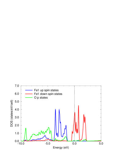
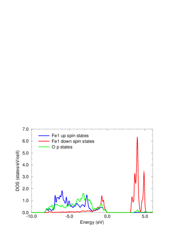
Figure 1: (Color online; adapted from Ref. cococcioni05 ) The density of states (DOS) of Fe₂SiO₄ fayalite obtained with GGA (top graph) and GGA+U (bottom graph). For the sake of clarity, only the contributions from the $d$ states of one of the Fe atoms and of the $p$ states of one of the O atoms are shown. These data were obtained in a study published in Ref. cococcioni05 .

Occasionally, finite band gaps are obtained as a result of crystal field splittings or Hund’s rule (as in NiO and MnO, respectively); however, even in these circumstances, they are underestimated by DFT, compared to experiments. In some cases (with degenerate states at the top of the valence band) the opening of a gap in the band structure through the Hubbard correction requires lowering the electronic subsystem to have a lower symmetry than the crystal, as discussed below.

The opening of a gap in the band structure is only one particular aspect of the effect the Hubbard correction has. Consistently with the predictions of the Hubbard model, the explicit account of on-site electron-electron interactions also favors electronic localization and the onset of an insulating ground state (provided the on-site Coulomb repulsion prevails on the kinetic term of the energy, minimized by electronic delocalization). One example is shown in Fig. 2 that visualizes the density of state (DOS) and the charge density of the highest energy state in CeO₂ with an oxygen vacancy fabris05 ; fabris05_1 . It is evident from the figure that, while GGA predicts the extra charge induced by the oxygen vacancy to be spread among the four Ce atoms around the vacancy and to be described by a delocalized state within the conduction band (top panel), the Hubbard correction induces the localization of the extra two electrons on the atomic $f$ orbitals of two of the Ce atoms around the defect that correspond to a state well localized within the gap of the pristine material. These results were obtained with a Wannier function-based implementation of the LDA+U (to be discussed later in this article) that also predicted the crystal structure and the DOS of reduces surfaces of CeO₂ and Ce₂O₃ in very good agreement with STM, AFM and photoemission experiments. If LDA or GGA were used, instead, the extra charge in the system associated with the O defect would be erroneously spread over the three outermost atomic layers, and the agreement with experimental results would significantly deteriorate fabris05 ; fabris05_1 .

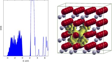
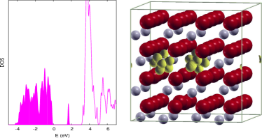
Figure 2: (Color online) Density of electronic states (DOS) and charge density of the gap state in a CeO₂ crystal with an oxygen vacancy (simulated by CeO_1.875). The shaded area in the DOS indicates occupied electronic states and the zero of the energy is fixed at the top of the valence band. The top and bottom panels show the results obtained with GGA and GGA+U, respectively. Results shown in this figure were obtained in a study published in Refs. fabris05 and fabris05_1 .

Similar calculations (albeit not based on Wannier functions) were also performed to study oxygen vacancies on reduced TiO₂ surfaces divalentin09 ; finazzi08 ; mattioli10 . These studies showed that the Hubbard correction was necessary to capture the localization of the extra charge on the $d$ states of the Ti atoms around the O vacancies and the consequent deformation of the crystal in its neighborood (polaronic self-trapment), although the quality of the results depend critically on the value of U and the way the Hubbard functional is used (e.g., with $U$ only on Ti $d$ or on Ti $d$ and O $p$ states).

II.2 Rotationally-invariant formulation

While able to capture the main essence of the LDA+U approach, the formulation presented in Eq. (II.1) is not invariant under rotation of the atomic orbital basis set used to define the occupation numbers $n^{I}_{m\sigma}$. Thus, calculations performed with this functional are affected by an undesirable dependence on the specific unitary transformation of the localized basis set chosen to define the atomic occupations, (Eq. (3)). A unitary-transformation-invariant formulation of LDA+U was introduced in Ref liechtenstein95 . In that work $E_{Hub}$ and $E_{dc}$ were given a more general expression, borrowed from the HF method:

$$E_{Hub}[\{n^{I}_{mm^{\prime}}\}]=$$

$$\frac{1}{2}\sum_{\{m\},\sigma,I}\{\langle m,m^{\prime\prime}|V_{ee}|m^{\prime},m^{\prime\prime\prime}\rangle n^{I\sigma}_{mm^{\prime}}n^{I-\sigma}_{m^{\prime\prime}m^{\prime\prime\prime}}+$$

$$(\langle m,m^{\prime\prime}|V_{ee}|m^{\prime},m^{\prime\prime\prime}\rangle-\langle m,m^{\prime\prime}|V_{ee}|m^{\prime\prime\prime},m^{\prime}\rangle)\times$$

$$n^{I\sigma}_{mm^{\prime}}n^{I\sigma}_{m^{\prime\prime}m^{\prime\prime\prime}}\}$$ (5)

$$E_{dc}[\{n^{I}_{mm^{\prime}}\}]=\sum_{I}\{\frac{U^{I}}{2}n^{I}(n^{I}-1)-$$

$$\frac{J^{I}}{2}[n^{I\uparrow}(n^{I\uparrow}-1)+n^{I\downarrow}(n^{I\downarrow}-1)]\}.$$ (6)

The invariance of the “Hubbard” term (Eq. (II.2)) stems from the fact that the interaction parameters transform as quadruplets of localized wavefunctions, thus compensating the variation of the (product of) occupations they are associated with. In Eq. (II.2), instead, the invariance is due to the dependence of the functional on the trace of the occupation matrices. In Eq. (II.2) the $V_{ee}$ integrals represent electron-electron interactions that are expressed as the integrals of the Coulomb kernel on the wave functions of the localized basis set (e.g., $d$ atomic states), labeled by the index $m$:

$$\langle m,m^{\prime\prime}|V_{ee}|m^{\prime},m^{\prime\prime\prime}\rangle=$$

$$\int d{\rm\bf r}\int d{\rm\bf r}^{\prime}\psi^{*}_{lm}({\rm\bf r})\psi_{lm^{\prime}}({\rm\bf r})\frac{e^{2}}{|{\rm\bf r}-{\rm\bf r}^{\prime}|}\psi^{*}_{lm^{\prime\prime}}({\rm\bf r}^{\prime})\psi_{lm^{\prime\prime\prime}}({\rm\bf r}^{\prime}).$$ (7)

Assuming that atomic (e.g., $d$ or $f$) states are chosen as the localized basis, these integrals can be factorized in a radial and an angular contributions. This factorization stems from the expansion of the Coulomb kernel in spherical harmonics (see Ref. liechtenstein95 and references quoted therein) and yields:

$$\langle m,m^{\prime\prime}|V_{ee}|m^{\prime},m^{\prime\prime\prime}\rangle=\sum_{k}a_{k}(m,m^{\prime},m^{\prime\prime},m^{\prime\prime\prime})F^{k}$$ (8)

where $0\leq k\leq 2l$ ($l$ being the angular quantum number of the localized manifold with $-l\leq m\leq l$). The $a_{k}$ represent the angular factors and correspond to products of Clebsh-Gordan coefficients:

$$a_{k}(m,m^{\prime},m^{\prime\prime},m^{\prime\prime\prime})=$$

$$\frac{4\pi}{2k+1}\sum_{q=-k}^{k}\langle lm|Y_{kq}|lm^{\prime}\rangle\langle lm^{\prime\prime}|Y^{*}_{kq}|lm^{\prime\prime\prime}\rangle.$$ (9)

The quantities $F^{k}$ are the (Slater) integrals involving the radial part of the atomic wave functions $R_{nl}$ ($n$ indicating the atomic shell they belong to). They have the following expression:

$$F^{k}=e^{2}\int d{\rm\bf r}\int d{\rm\bf r}^{\prime}r^{2}r^{\prime 2}R_{nl}^{2}({\rm\bf r})\frac{r^{k}_{<}}{r^{k+1}_{>}}R_{nl}^{2}({\rm\bf r}^{\prime})$$ (10)

where $r_{<}$ and $r_{>}$ indicate, respectively, the shorter and the larger radial distances between $r$ and $r^{\prime}$. For $d$ electrons only $F^{0}$, $F^{2}$, and $F^{4}$ are needed to compute the $V_{ee}$ matrix elements (for higher $k$ values the corresponding $a_{k}$ vanish) while $f$ electrons also require $F^{6}$. Consistently with the definition of the dc term (Eq. (II.2)) as the mean-field approximation of the Hubbard correction (Eq. (II.2)), the effective Coulomb and exchange interactions, $U$ and $J$, can be computed as atomic averages of the corresponding Coulomb integrals over the localized states of the same manifold (in this example atomic orbitals of fixed $l$). For $d$ orbitals it is easy to obtain:

$$U=\frac{1}{(2l+1)^{2}}\sum_{m,m^{\prime}}\langle m,m^{\prime}|V_{ee}|m,m^{\prime}\rangle=F^{0}$$ (11)

$$J=\frac{1}{2l(2l+1)}\sum_{m\neq m^{\prime},m^{\prime}}\langle m,m^{\prime}|V_{ee}|m^{\prime},m\rangle=\frac{F^{2}+F^{4}}{14}.$$ (12)

Although strictly valid for atomic states and unscreened Coulomb kernels, these equations have often been adopted to evaluate screened Slater integrals: once $U$ and $J$ are computed from the ground state of the system of interest, the $F^{k}$ parameters (and the $V_{ee}$ integrals) are extracted using Eqs. (11) and (12) based on the assumption that the ratio between them has the same value as for atomic states (e.g., $F_{2}/F_{4}=0.625$). The limits of this assumption were thoroughly discussed in Ref vaugier12 .

II.3 A simpler formulation

The one presented in section II.2 is the most complete formulation of the LDA+U, with fully orbital-dependent electronic interactions. However, in many occasions, a simpler expression of the Hubbard correction ($E_{Hub}$), introduced in Ref. dudarev98 , is actually adopted and implemented. This simplified functional can be obtained from the full formulation discussed in section II.2 by retaining only the lowest order Slater integrals $F^{0}$ and neglecting all the higher order ones: $F^{2}=F^{4}=J=0$. This simplification corresponds to assuming that $a_{0}(m,m^{\prime},m^{\prime\prime},m^{\prime\prime\prime})=\delta_{m,m^{\prime}}\delta_{m^{\prime\prime},m^{\prime\prime\prime}}$. Using these conditions in Eqs. (II.2) and (II.2), one easily obtains:

$$E_{U}[\{n^{I\sigma}_{mm^{\prime}}\}] = E_{Hub}[\{n^{I}_{mm^{\prime}}\}]-E_{dc}[\{n^{I}\}]=$$ (13)

$$= \sum_{I}\frac{U^{I}}{2}\left[\left(n^{I}\right)^{2}-\sum_{\sigma}{\rm Tr}~{}[({\rm\bf n}^{I\sigma})^{2}]\right]$$

$$- \sum_{I}\frac{U^{I}}{2}n^{I}(n^{I}-1)$$

$$= \sum_{I,\sigma}\frac{U^{I}}{2}{\rm Tr}~{}[{\rm\bf n}^{I\sigma}(1-{\rm\bf n}^{I\sigma})].$$

It is important to stress that the simplified functional in Eq. (13) still preserves the rotational invariance of the one in Eqs. (II.2) and (II.2), through its dependence on the trace of occupation matrices and of their products. On the other hand, the formal resemblance to the HF energy functional is lost in this formulation and only one interaction parameter ($U^{I}$) is needed to specify the corrective functional. It is also worth remarking that, when a non-orthogonal basis set is used to define atomic occupations, the rotational (tensorial) invariance of the Hubbard energy requires the use of a covariant-controvariant formulation (which won’t be detailed in this article), as explained in Ref. oregan11 .

The simplified version of the Hubbard correction, Eq. (13), has been succesfully used in several studies and for most materials it yields similar results as the fully rotationally invariant one (Eq. (II.2) and (II.2)). Some recent literature has shown, however, that the explicit inclusion of the Hund’s rule coupling $J$ is crucial to describe the ground state of systems characterized by non-collinear magnetism spaldin10 ; pickett06 , to capture correlation effects in multiband metals demedici11 ; georges11 , or to study heavy-fermion systems, typically characterized by $f$ valence electrons and subject to strong spin-orbit couplings spaldin10 ; pickett06 ; bultmark09 . A recent study nakamura09 also showed that in some Fe-based superconductors a sizeable $J$ (possibly exceeding the value of $U$) is needed to reproduce (within LDA+U) the experimentally measured magnetic moment of Fe atoms. Several different flavors of corrective functionals with exchange interactions were also discussed in Ref. ylvisaker09 .

Due to the spin-diagonal form of the simplified LDA+U approach in Eq. (13), it has become customary to attribute the Coulomb interaction $U$ an effective value that incorporates the exchange correction: $U_{eff}=U-J$. This practice has been introduced in the original formulation of the simplified functional, in Ref. dudarev98 . As discussed in section VI.2, this assumption is actually not completely justifyable as the resulting functional neglects other interaction terms (proportional to $J$) that are of the same order as the ones responsible for the negative correction to the on-site Hubbard $U$ for parallel-spin electrons.

II.4 Theoretical background and practical remarks

The previous parts introduced the general formulation of the LDA+U functional and reviewed the most widely used implementations. This section is devoted to clarifying in a more detailed way its theoretical foundation (possibly in comparison with other corrective methods), to discussing the possibility to use this tool for the study of various classes of systems and to assessing the conditions under which it can be expected to be most predictive. While useful for a more precise theoretical framing of the method, this part is not essential to understand how LDA+U is implemented in DFT codes and how it works in actual calculations.

II.4.1 LDA+U vs Hartree-Fock and Exact Exchange

The expression of the full rotationally invariant Hubbard functional (Eqs. (II.2)) shows a quite clear resemblance with the Hartree-Fock (HF) energy. Therefore, what the LDA+U correction does could be understood as a substitution of mean-field-like density-density electronic interactions, contained in the approximate exchange-correlation (xc) functional, with a HF-like Hamiltonian. This is much in the same spirit of hybrid functionals in which the exchange part of the xc functional is shaped as a Fock operator (multiplied by a screening factor) constructed on KS states. Some notable differences from HF are, however, to be stressed: $i)$ the effective interactions in the LDA+U functional are screened, rather than based on the bare Coulomb kernel (as in HF); $ii)$ the LDA+U functional only acts on a subset of states (e.g., localized atomic orbitals of $d$ or $f$ kind), rather than on all the states in the system; $iii)$ due to the marked localization of the orbitals the Hubbard functional acts on, the effective interactions are often assumed to be orbital-independent so that, in the simpler formulation of Eq. (13), they are substituted by (or computed from) their atomic averages, Eqs. (11) and (12). This assumption, justified by the fact that more localized states retain their atomic character (and spherical symmetry) to a higher extent, (partially) looses its validity in presence of crystal field or spin-orbit interactions that can lift the degeneracy (and equivalence) of localized orbitals. Although the use of Fock integrals make hybrid functionals appear a more systematic and accurate method to correct some of the above-mentioned flaws of approximate DFT, their calculation incurr in significantly higher computational costs. Furthermore, hybrid functionals also depend on a parameter (as the Hubbard $U$ is often seen for LDA+U), namely the amount of Fock-exchange (mixing coefficient) to be included in the xc functional. The quality of the results can depend sensibly on this parameter that needs to be chosen for each system. This quantity is generally determined semi-empirically (e.g., through fitting of the properties of a large variety of different systems)feng04 , or through a material-dependent optimization, (e.g., by an iterative procedures, as proposed in Ref. marom12 ). Although this mixing coefficient results usually in the 0.2 - 0.3 range, there is no universal value that can be used with all the systems, nor a precise physical meaning attached to it except, perhaps, the not so precisely quantified attenuation of the exchange interaction due to the correlation part of the functional.

The formal similarity with a HF functional may arise some suspect about the possibility to use LDA+U (and hybrid functional) to improve the description of correlated systems. In fact, by definition, HF does not account for electronic correlation and it is quite unrealistic that the complexity of the many-body problem can be captured by the screening of the effective electronic interactions. However, it should be noted that the LDA+U functional, besides still containing a correlation term in the LDA part, operates the Hubbard correction on KS wave functions. These are not associated to any physical meaning other than being constrained to reproduce the exact charge density of the system. On the other hand, the single particle wave functions that are optimized during the self-consistent solution of the Hartree-Fock equations are the ones that minimize the energy of the system in the hypothesis that the ground state many-body wave function is the single Slater determinant that can be constructed out of them. While this is an important difference, the question of whether a HF-like corrective functional acting on the KS orbitals can effectively improve (with respect to approximate exchange correlation functionals) the description of the ground state of correlated systems remains open. Aiming more to a qualitative argument than a conclusive answer, we can observe that if a gap is present in the single-particle (KS) energy spectrum of a system, the occupations of the corresponding energy levels are all 1 or 0, depending on whether the state is in the valence or in the conduction manifold, respectively, and the ground state charge density can be obtained from a single Slater determinant constructed with the fully occupied orbitals. In these circumstances, it is reasonable to expect that a correction formally shaped as a HF energy functional could be effective in improving the representation of the correlated ground state by tuning the width of the energy gap in the single-electron energy spectrum (possibly incorporating the xc potential discontinuity) and favoring integer occupations of the states at the edge of valence and conduction bands. This action can be expected to affect also other physical properties (as, for example, the equilibrium crystal structure and the vibrational spectrum) of the material through the modifications it brings to its electronic structure (charge density). As documented in abundant literature (see, for example, Refs. anisimov91_2 ; anisimov93_1 ; dudarev98 ; bengone00 ; martin02 ; feng04 ; towler94 ), LDA+U and HF (or hybrid functionals) obtain, in fact, a quite good representation of the ground state properties of correlated systems (e.g., transition metal oxides), provided a gap is present in the KS spectrum (e.g., because of crystal field), as in NiO and MnO. When this is not the case and the degeneracy of frontier valence states (closest to the Fermi level) results in fractional occupations and absence of band gaps, a preliminary symmetry breaking is usually required to create the optimal conditions under which these corrections are most effective. However, this preliminary “preparation” of the system has some theoretical and practical implications that will be discussed for the case of FeO in one of the following sections.

II.4.2 Potential discontinuity, band gap and energy linearization

Improving the estimate of the band gap is one of the original objectives of the LDA+U anisimov93_1 ; solovyev94 and can be shown to also address (albeit in an approximate way) well-known flaws of approximate energy functionals, such as the lack of a discontinuity in the xc potential (as discussed after Eq. (4)). To see this, let us consider a $N$-electron isolated system. The fundamental gap is defined as the difference between the ionization potential $I$ and the electron affinity $A$:

$$E_{g} = I-A$$ (14)

$$= [E(N-1)-E(N)]-[E(N)-E(N+1)]$$

$$= E(N+1)+E(N-1)-2E(N)$$

where $E(N)$, $E(N+1)$ and $E(N-1)$ are the total energy of the system in its neutral state and with one electron added to or removed from its orbitals, respectively. It is important to note that the one in the last line of Eq. (14) is a finite-difference approximation of the second derivative of the total energy with respect to the number of electrons. This observation will be useful to understand some approaches to compute the effective interaction $U$ of the Hubbard functional that will be discussed in section III. Based on the expression of the DFT total energy it can be shown (see, e.g., Ref grosslibro ) that:

$$E_{g}=\Delta_{KS}+\Delta_{xc}$$ (15)

where the first term corresponds to the energy gap between the HOMO and the LUMO states from the KS energy spectrum,

$$\Delta_{KS}=\epsilon^{LUMO}_{N}-\epsilon^{HOMO}_{N},$$ (16)

while the second represents the discontinuity in the exchange-correlation potential computed for the neutral system grosslibro :

$$\Delta_{xc}=\frac{\delta E_{xc}[n]}{\delta n({\rm\bf r})}|_{N+\delta}-\frac{\delta E_{xc}[n]}{\delta n({\rm\bf r})}|_{N-\delta},$$ (17)

where the derivatives are evaluated for densities that integrate to $N+\delta$ and $N-\delta$ electrons, respectively, and the limit $\delta\rightarrow 0+$ is implied. The discontinuity of the xc potential is a property of the exact DFT functional which is of fundamental importance to describe, for example, molecular dissociations and electron-transfer processes perdew82 ; perdew83 . In extended systems a discontinuity in the xc potential is also expected for insulating ground states. The fundamental gap can be defined in a similar way as for isolated systems, as the difference between the total energies obtained from calculations with a fraction of electron per unit cell in eccess or in defect with respect to the neutral crystal and compensated by a jellium charge grosspra09 ; chan10 . Most of approximate exchange-correlation functionals, however, miss the discontinuity of the xc potential $\Delta_{xc}$ and yield an analytical dependence of the total energy on $N$.

As illustrated in the discussion after Eq. (4), the Hubbard correction introduces a discontinuity in the potential acting on the orbitals of the localized basis set, whose amplitude is approximately $U$. Therefore, if these localized states are the ones at the borders of valence and conduction manifolds (usually the case for systems this correction is applied to), and the value of $U$ is appropriately chosen, the Hubbard energy functional can be used to reintroduce the discontinuity in the exchange-correlation potential. In particular, since the correction modifies the KS potential, the discontinuity is introduced in the single particle spectrum as well and the KS band gap obtained with the corrected functional can be expected to match the fundamental gap: $\epsilon_{LUMO}^{LDA+U}-\epsilon_{HOMO}^{LDA+U}\approx\Delta_{KS}+\Delta_{xc}$. It is important to remark that this is not a feature of the exact KS theory. Because of this difference, LDA+U could be classified as as a “generalized Kohn-Sham” theory.

The introduction of the exchange-correlation potential discontinuity is also related to (and is the necessary condition for) the linearization of the total energy profile as a function of the number of electrons. As explained in abundant literature (see, for example, Refs. grosslibro ; perdew82 ; levy82 ; yang98 ; yang00 ) a piece-wise linear profile of the energy is characteristic of systems able to exchange electrons with a reservoir of charge. In this context, a fractional number of electrons on the orbitals of these systems is to be interpreted as resulting from a mixture of states with different integer occupations. With the exact xc functional the resulting ground state energy would be the linear combination of those corresponding to nearest integer number of electrons.

The linearizing action of the Hubbard functional on the approximate DFT energy is more evident in its simpler formulation, Eq. (13), that consists of subtracting a quadratic term and adding a linear one. It is important to stress that the “+U” correction linearizes the energy with respect to on-site occupations, rather than the total number of electrons. However, localized orbitals (e.g., $d$ or $f$) can be thought of as belonging to isolated atoms immersed in a “bath” of delocalized states. In addition, they typically belong to open shells and thus represent the frontier states whose occupation changes when the total number of electrons is varied. Therefore, the linearization of the energy with respect to the atomic occupations is a legitimate operation.

The elimination of the (spurious) curvature of the energy profile also makes the Hubbard functional look similar to a self-interaction correction (SIC) perdew81 . In fact, a SIC functional could be easily obtained from the diagonal term of the exact exchange contained in hybrid functionals, whose analogy with LDA+U has already been highlighted. This similarity has also been amply discussed in the context of Koopmans-corrected DFT functionals dabo09 ; dabo10 and won’t be further expanded here. It is worth to stress, however, that LDA+U only corrects localized states, for which self-interaction is generally expected to be stronger. The formal similarity with SIC and hybrid functionals suggests that LDA+U should be also effective in correcting the underestimated band gap of covalent insulators (e.g., Si, Ge, or GaAs), for which the former have often been successfully used. Indeed, while the “standard” “+U” functional (Eq. 13) is not effective on these systems, a generalized formulation of the Hubbard correction with inter-site couplings proves able to achieve this result, as will be discussed in section VI.1.

II.4.3 Degenerate ground states: the case of FeO

The orbital independence of the effective electronic interaction, allows to regard the positive-definite “+U” correction in Eq. (13) as a penalty functional that forces the on-site occupation matrix (Eq. (3)) to be idempotent. This action corresponds to favoring a ground state described by a set of KS states with integer occupations (either 0 or 1). and to imposing a finite gap in the single-particle (Kohn-Sham) energy spectrum. While this is another way to see how the “+U” correction helps improving the description of insulators, it should be kept in mind that the linearization of the energy as a function of orbital occupations is a more general and important effect to be obtained. In fact, in case of degenerate ground states, fractional occupations (resulting, effectively, in a metallic KS system) can, in principle, represent linear combinations of insulating ground states, each having different sets of equivalent single-particle states occupied (and a lower symmetry than their sum). In these cases the total energy should be equal to the corresponding linear combination of the energies of the single insulating ground states. In these situations, an insulating KS system should not be expected/pursued unless the symmetry of the electronic state is decreased and the system “prepared” in one of the equivalent insulating ground states of lower symmetry.

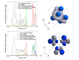
Figure 3: (From Ref. cococcioni05 ; color online). Projected density of states and highest energy occupied orbital of FeO (top) in the unbroken symmetry (upper panels) and broken symmetry states (lower panels).

Transition metal oxides with nearly half-filled or full $d$ shells, as FeO and CuO, are well known examples of materials with degenerate insulating ground states. The case of CuO will be discussed in section VI.2. In FeO all the Fe ions are in their high magnetization configuration with (nominally) five $d$ electrons in the majority-spin states and one in their minority spin counterparts. Because of the rhombohedral symmetry of the crystal and the consequent crystal field splitting of the $d$ energy levels, the minority spin electron occupies two almost degenerate groups of states composed, respectively, by a $z^{2}$ state ($z$ being the rhombohedral axis) and a doublet of states (mostly of $x^{2}-y^{2}$ and $xy$ symmetry with $x$ and $y$ on the (111) planes of the lattice). This degeneracy leads to a ground state associated with a metallic KS system. If LDA+U is used, the total energy is minimized when the doublet degeneracy is lifted (through lowering the rhombohedral symmetry by a tripartition of the metal sublattice) and the minority spin electron is hosted on a combination of $d$ states extending on the (111) planes cococcioni05 , as illustrated in Fig. 3 (lower panel). This solution is actually not unique: in fact, at least three distinct linear combinations (orbital orders) of $d$ states exist, all hosting the minority spin electrons of Fe on (111) planes, that are equivalent and degenerate. Each of them is predicted to be insulating thanks to the lifting of the degeneracy between the states in the doublet group and to the discontinuity in the potential introduced by the Hubbard correction. However, the ground state of the system should be regarded as a linear combination (with equal weights) of these solutions which, in fact, recovers the full rhombohedral symmetry of the crystal. An insulating state, with the minority spin $d$ electrons of Fe hosted on the $z^{2}$ state (along [111]), preserves the rhombohedral symmetry, but has higher energy. In Ref. cococcioni05 it was shown that each of the equivalent ground states with broken symmetry can predict the rhombohedral distortion of the crystal under pressure in better agreement with experiments willis53 ; yagi85 than DFT or GGA+U ground states with full rhombohedral symmetry. This result is shown in Figure 4 that reports the variation of the rhombohedral angle of FeO under pressure and compares the results obtained with GGA (red line), GGA+U with rhombohedral symmetry (green line) and GGA+U in the broken symmetry phase (blue line). This conclusion is in agreement with the results of Ref. gramsh03 , although the ground state stabilized by LDA+U seems to have a different symmetry (and different orbital order) than the one predicted in Ref. cococcioni05 .

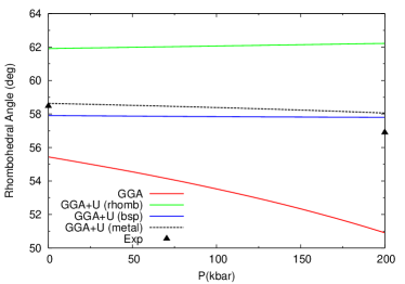
Figure 4: (Adapted from Ref. cococcioni05 ; color online). The rhombohedral angle of FeO as a function of pressure. The solid blue line describes GGA+U results in the broken-symmetry phase (bsp), the red one GGA, the green GGA+U in the rhombohedral symmetry. The dotted line is from GGA+U calculations with a metallic KS spectrum (see text). Diamonds represent the (extrapolations from) experimental data willis53 ; yagi85 .

The necessity to break the symmetry of the electronic system to reach its insulating ground state has also been stressed in Ref. dorado09 where LDA+U is used to study the electronic and structural properties of UO₂. In this work it is also shown that, favoring the anisotropy of localized states, LDA+U often induces the formation of metastable phases in which the system can get trapped. To avoid this inconvenience, a preconditioning of the occupation matrices (and of the Hubbard potential) is sometimes needed.

If the rhombohedral symmetry is not broken to allow for the localization of the minority spin electron of Fe on one of the (111)-planar $d$ states, this electron is equally shared by them resulting in a metallic KS spectrum. If the GGA+U is used on this ground state the dotted line of Fig. 4 is obtained. The good agreement with experimental data and with other GGA+U results in the broken symmetry phase is a confirmation of the idea that the linearization of the energy with respect to the occupation of degenerate states is effective even in cases where no gap appears in the KS single-particle spectrum. A more accurate theoretical analysis shows that this less “orthodox” use of LDA+U (on the fully symmetric and metallic ground state) is less accurate and should be trusted only in cases where the degeneracy that is responsible for the metallic character is not lifted by the deformation.

In some cases, where the degenerate states are quantistically entangled, the breaking of symmetry could have negative consequences on the description of some physical properties and should be imposed with care (if at all). In these cases the use of the Hubbard correction on a degenerate (metallic) state could actually be a better option. A typical example of this type of situations is represented by open-shell singlet molecules, typically affected by the problem of spin contamination. Section VI.1 reports the case of the Ir(ppy)₃ dye (discussed more extensively in Ref. himmetoglu12_2 ) whose open shell excited singlet state is best captured (in consistency with the Slater half-occupation theorem slater72 ) by a configuration having half electron of each spin promoted to the LUMO of the molecule which, in a KS (or band structure) picture, corresponds to a metallic state.

In the case of FeO, discussed above, after the spin symmetry is broken and an antiferromagnetic ground state is obtained, a finite gap in the KS spectrum is obtained after lowering the rhombohedral symmetry of the crystal and breaking the equivalence of $d$ orbitals on the same (111) plane. In CuO, described in section VI.2 of this review, the breaking of the symetry is somewhat harder to obtain as spin and orbital degeneracies reinforce each other. Other transition metal mono-oxides, as NiO, only require spin symmetry breaking (AF ground state) as a (small) gap appear in their KS spectrum due to crystal field. Spin degeneracies also need to be lifted in paramagnetic insulators if a gap in the KS band structure is to be obtained with LDA+U.

The necessity to lower or break the symmetry of the electronic system to obtain an insulating single particle spectrum descends from the degeneracy of the ground state of many correlated materials (e.g., transition metal oxides) and in the multi-reference character of their wave function dimarco12 , whose implications cannot be capture by the straight use of LDA+U on the fully symmetric ground state. More sophisticated methods and corrective approaches, as RDMFT and DFT+DMFT are able to describe degenerate insulators without explicitly lowering the symmetry of the system and can be used to capture metal-to-insulator phase transitions (see, for example, Refs. held01 ; shorikov10 ; sharma13 ). It is significant that these corrective approaches can be shown to also introduce a finite discontinuity in the chemical potential of the system (the corresponding quantity of the potential in a KS framework) grossepl07 ; grosspra09 .

II.4.4 Other flaws and merits of LDA+U

At this point, it is important to highlight also other approximations inherent to the LDA+U description of correlated ground states. Atomic states are treated as effectively localized and their dispersion is neglected, as is the k-point dependence of the effective interaction (the Hubbard $U$). This limit can be alleviated, in part, by taking into account inter-site electronic interactions as explained in Ref. campo10 and in section VI.1 of this review. Another aspect to remark is the fact that LDA+U corresponds to a static correction. In fact, it neglects the frequency dependence of the effective electronic interaction (i.e., of its screening). The numerical difference between statically and dynamically screened effective interactions was already pointed out in Ref. springer98 , that focused on bulk Ni as a case study. In Ref. sasioglu11 the constrained RPA approach arya04 is used to evaluate the Hubbard $U$ in transition metals and to stress the importance of its dependence on frequency for these materials. The variation of $U$ with $\omega$ suggests that the static LDA+U is probably not very accurate for many systems of this type. A possible correction to static models that allows to (partially) account for the frequency dependence of $U$ at low energies ($\omega<\Lambda$ where $\Lambda$ represents the bandwidth of the system) was already proposed in Ref. arya04 . Ref. casula12 has recently discussed the meaning and the importance of using a frequency-dependent Hubbard $U$. In order to account for dynamical effects on correlation (e.g., the frequency dependence of the screening of effective interaction by delocalized electrons) more sophisticated approaches are needed such as, for example, DFT+DMFT metzner89 ; muller89 ; brandt89 ; janis91 ; georges92 ; georges96 , that has been shown to be able to describe metals and Mott insulators and to capture correlation-driven phenomena as metal-to-insulator transitions (see, e.g., Refs. held01 ; shorikov10 ). LDA+U, that can be considered the static (Hartree-Fock-like) limit of DFT+DMFT, can not capture dynamical fluctuations and can lead to qualitatively wrong results in systems, as many rare-earth compounds, where these play an important role in determining both ground and excited state properties as, for example, the strength of hybridization between orbitals or the quasi-particle excitation energies pourovskii05 ; suzuki09 . Unfortunately, DFT+DMFT is significantly more computationally demanding than LDA+U and, while inherently superior in describing multi-reference ground states, it is hardly usable or quite impractical for large systems, for molecular dynamics or for large-scale calculations as, for example, those screening and comparing the total energy of large numbers of different materials and structural phases. Furthermore, DFT+DMFT accounts for electronic correlation using a Hubbard model (solved within the DMFT approximation) wherein each correlated atom is treated as an Anderson impurity in contact with the “bath” represented by the rest of the crystal. Therefore, it shares with LDA+U the dependence of its results on the choice of the interaction parameter $U$ and on the specific double-counting term used to compensate for the correlation energy already contained in the LDA Hamiltonian. Other problematic aspects of DFT+DMFT are instead inherent to the approximations made in solving the Anderson impurity model such as, the finite sampling of the Greens functions on the frequency axis, the lack of self-consistency over the charge density, or the overlook of spatial fluctuations, sometimes cured through the cluster (or cellular) DMFT approach (cDMFT) lic00 ; kotliar01 ; senechal12 . The effects of these approximations will not be further discussed here and the reader is encouraged to review publications dedicated to the DFT+DMFT method (e.g., Ref. pavarinibook11 and references quoted therein).

The small computational cost of LDA+U and the significant improvement it brings to the KS eigenvalues towards their interpretation as single-particle excitation energies have promoted its use in conjunction with methods to compute excitation energies: time-dependent DFT (TDDFT) runge84 ; burke05 and GW hedin65 . The use of TDDFT on extended (crystalline) systems can be quite challenging due to the inability of the (approximate) interaction kernels to capture important long-range interactions sottile05 ; botti07 . Starting TDDFT calculations from a LDA+U functional has proven effective to circumvent this problem and to compute the bound $d-d$ Frenkel excitons in NiO (using a Wannier function basis set) ku10 in quite good agreement with experimental results larson07 ; muller08 . The theoretical relationship between LDA+U and GW methods has been discussed in Ref. anisimov97 . The incorporation of the potential discontinuity in the KS gap has opened the possibility to interpret LDA+U wave functions and KS energies as zeroth-order estimates of their quasi-particle counterparts. Therefore, when applied to a LDA+U reference Hamiltonian, the GW correction, needed to recover the physical value of these quantities, is smaller than with approximate DFT functionals and the simplest approximations (most commonly, G₀W₀) become inherently more accurate. In fact, LDA+U/G₀W₀ has been succesfully used to calculate the quasi particle spectrum of several systems jiang09 ; scheffler10 ; toroker11 ; kanan12 ; patrick12 ; liao11 ; isseroff12 ; kioupakis08 , often improving the results of LDA/G₀W₀.

The negligible computational overload associated with LDA+U also makes it a precious (often the only affordable) method for ab initio calculations aimed at screening large sets of correlated materials to either scout new compounds and phases or to optimize the properties of existing ones for target applications. A typical approach to computational materials design, the high-throughput (HT) technique is a clear example of this type of application of LDA+U. HT is based on the efficient construction of a database of known/computed materials and on a smart data mining technique to select or design optimal candidate systems for target properties curta03 ; fischer06 . LDA+U can be easily implemented and used in HT searches based on DFT calculations. A recent implementation of LDA+U in HT curta11 ; curta12 ; curta13 has demonstrated that a better description of electronic correlation is very useful to make reliable predictions on the properties of correlated materials. Although a qualitative improvement of results over approximate DFT functional is often obtained for correlated materials, the quantitative outcome of LDA+U calculations depends on the value of the Hubbard $U$. For a full exploitation of the potential of HT calculations, an automatic (and run-time) evaluation of this interaction parameter would be highly desirable. Some approaches to obtain the value of $U$ from ab initio calculations are discussed and compared in the next section.

III Computing the Hubbard $U$

III.1 The necessity to compute $U$

From the expression of the Hubbard functionals discussed in previous sections, it is natural to expect the results of the LDA+U method to sensitevely depend on the numerical value of the effective on-site electronic interaction, the Hubbard $U$. A tendency wide-spread in literature is to use this approach for a rough assessment of the role of electronic correlation; therefore, it has become common practice to tune the value of $U$ in a semiempirical way, through seeking agreement with available experimental measurement of certain properties and using the so determined value to make predictions on other aspects of the behavior of systems of interest. Besides being not satisfactory from a conceptual point of view, this practice does not allow to appreciate the variations of the on-site electronic interaction $U$ during chemical reactions, structural/magnetic transitions or, in general, under changing physical conditions. As demonstrated in literature kulik06 ; hsu11 , instead, to capture the variation of the electronic interactions is crucial for modeling in a quantitatively predictive way the above mentioned situations. Therefore, in order to exploit all the potential of this approach it is very important to define a procedure to compute the Hubbard $U$ in a consistent and reliable way. The interaction parameters should be calculated for every atom the Hubbard correction is to be used on, for the considered crystal structure and the specific magnetic ordering of interest. The obtained value depends not only on the atom, its crystallographic position in the lattice, the structural and magnetic properties of the crystal, but also on the localized basis set used to define the on-site occupation in the “+U” functional. Therefore, contrary to another quite common practice, the effective interactions have limited portability and their values should not be extended from one crystal to another, or from one implementation of LDA+U to another but, rather, recomputed each time.

III.2 A brief literature survey

In several works on LDA+U (see, e.g., Ref. anisimov91 ), based on the use of localized basis sets and on the Atomic Sphere Approximation (ASA), the Hubbard $U$ is computed from the variation of the total energy upon changing by one electron the population of the localized (e.g., 3$d$) states of a single atom:

$$U \approx E\left(\frac{n}{2}+1;\frac{n}{2}\right)-E\left(\frac{n}{2};\frac{n}{2}\right)$$ (18)

$$- E\left(\frac{n}{2}+1;\frac{n}{2}-1\right)+E\left(\frac{n}{2};\frac{n}{2}-1\right).$$

In this equation the two numbers in between parenthesis represent the population of the two spin manifolds and the original configuration is spin unpolarized with $n$ electrons on the $d$ shell of each atom. In practice, this quantity is evaluated (thanks to the Janak theorem janak78 ) from the difference between $3d$ energy levels:

$$U\approx\tilde{\epsilon}_{3d}\left(\frac{n}{2}+\frac{1}{2};\frac{n}{2}\right)-\tilde{\epsilon}_{3d}\left(\frac{n}{2}+\frac{1}{2};\frac{n}{2}-1\right)$$ (19)

where $\tilde{\epsilon}(x,y)=\epsilon(x,y)-\epsilon_{F}(x,y)$ ($\epsilon_{F}$ representing the Fermi level). In the expression of Eq. (19) the screening from the other (e.g., $s$ and $p$) states is automatically included by letting their population reorganize when changing the number of electrons on $d$ states. From a comparison between Eqs. (18) - (19) and Eq. (14) it is easy to realize that the $U$ is computed as the effective second derivative of the energy with respect to the occupation of the $d$ orbitals. To ensure that the computed $U$ does not contain contributions from the hopping terms (explicitly accounted for at run-time) the hopping between the $d$ states of the perturbed atom and other states in the crystal is explicitly eliminated. This procedure ensures that the computed $U$ corresponds to the amplitude of the potential discontinuity, $\Delta_{xc}$, and that the gap in the LDA+U KS spectrum has a width equal to the fundamental gap of the system. The possibility to change the occupation of $d$ states and to cut hopping terms with other states are quite specific to implementations that use localized basis sets (e.g., LMTO); other implementations (e.g., using plane waves) require different procedures to compute the effective interaction parameters pickett98 that will be discussed below.

Another method to compute the Coulomb and exchange parameters for DFT+U calculations has been recently proposed in Ref. mosey07 . In this work $U$ and $J$ are evaluated by projecting unrestricted HF molecular orbitals onto atomic orbitals and retaining only on-site (intra-atomic) terms from the Hartree Fock interactions, averaged over the states (of specific angular momentum) of the same atom. While consistent with the HF-like expression of the DFT+U corrective functional, this method yields values for $U$ and $J$ that are somewhat higher than those obtained from other methods, probably due to the use of unscreened Coulomb (and exchange) integrals from UHF. Screening is instead accounted for in other approaches described below.

One of the latest methods to compute the effective (screened) Hubbard $U$ is based on constrained RPA (cRPA) calculations springer98 ; arya04 ; arya06 ; vaugier12 ; sasioglu12 and has become particularly popular within the DFT+DMFT community. This approach yields a fully frequency-dependent interaction parameter that is efficiently screened by “non Hubbard” orbitals. If the polarization of the system is written as the sum of a term from localized (e.g., $d$) states, and one from delocalized ones: $P({\rm\bf r},{\rm\bf r}^{\prime})=P_{d}({\rm\bf r},{\rm\bf r}^{\prime})+P_{r}({\rm\bf r},{\rm\bf r}^{\prime})$, the inverse dielectric function can be factorized as follows: $\epsilon^{-1}=\epsilon_{r}^{-1}\epsilon_{d}^{-1}$. The effective interaction acting on the $d$ (localized) manifold can then be computed from the screening of the electronic interaction kernel due to the reorganization of electrons on extended states. The dielectric function, responsible for this screening, can be defined as follows:

$$\epsilon_{r}({\rm\bf r},{\rm\bf r}^{\prime})=\delta({\rm\bf r},{\rm\bf r}^{\prime})-\int P_{r}({\rm\bf r},{\rm\bf r}^{\prime\prime})f_{Hxc}({\rm\bf r}^{\prime\prime},{\rm\bf r}^{\prime})d{\rm\bf r}^{\prime\prime}.$$ (20)

In this expression $f_{Hxc}({\rm\bf r}^{\prime\prime},{\rm\bf r}^{\prime})$ is the kernel of the Hartree and xc interactions: $f_{Hxc}({\rm\bf r},{\rm\bf r}^{\prime})=\frac{1}{|{\rm\bf r}-{\rm\bf r}^{\prime}|}+\frac{\delta v_{xc}({\rm\bf r})}{\delta\rho({\rm\bf r}^{\prime})}$ vaugier12 . Based on this definition, the effective interaction $W_{r}$ acting on the $d$ (localized) manifold can be computed as:

$$W_{r}=\epsilon_{r}^{-1}f_{Hxc}=\frac{f_{Hxc}}{1-P_{r}f_{Hxc}}.$$ (21)

The Hubbard $U$ is obtained as the expectation value of $W_{r}$ on the wave functions of the localized basis set arya04 ; arya06 . In actual calculations, based on the explicit evaluation of the polarization $P$ springer98 ; arya04 , only the Coulomb kernel is used (hence the name “constrained RPA”). This approximation is based on the assumption that the xc kernel, whose inclusion would make the procedure much more involved and demanding, is numerically less important than the Hartree one and can be safely neglected. From the procedure outlined above $U$ results the effective interaction partially screened by the degrees of freedom not explicitly included in the model Hamiltonian it is used in. In fact, the polarization $P_{r}$, necessary to compute $W_{r}$ (and $U$), is obtained subtracting from the total polarization $P$ the term $P_{d}$ due to $d-d$ transitions (the transitions between correlated $d$ states and non correlated ones are still included). The screening of the interaction due to $P_{d}$ is performed at run-time when solving the DFT+DMFT equations. From the definition of the dielectric function it is easy to show that, when the screening from $P_{d}$ is applied to $W_{r}$, the fully screened interaction is obtained: $W=\epsilon^{-1}f_{Hxc}=\epsilon_{d}^{-1}W_{r}$.

III.3 Computing $U$ from linear-response

III.3.1 Technical aspects and computational procedure

In this section we describe the linear response approach to the calculation of the effective Hubbard $U$ that was introduced in Ref. cococcioni05 . This method (inspired to the one proposed in Ref pickett98 ) has been implemented in the plane-wave pseudopotential total-energy code of the Quantum-ESPRESSO package giannozzi09 . As in the first method outlined above, and consistently with the definition and the intent of the Hubbard corrective functional, the $U$ is calculated from the spurious curvature of the (approximate DFT) total energy of the system as a function of the number of electrons on its localized (atomic) orbitals. In fact, as was briefly discussed in section II.4, when these localized states exchange electrons with the rest of the crystal (acting like a charge reservoir), the total energy obtained from approximate DFT xc functionals varies in an analytic way and its derivative (the effective potential acting on them) misses or significantly underestimates the discontinuity at integer occupations that corresponds to the fundamental gap of the system (Eq. (15)). As demonstrated by quite abundant literature perdew-par82 ; levy82 ; perdewlevy83 , the energy profile should consist, instead, of a series of straigth segments joining the energies corresponding to integer occupations. A visual comparison between the exact (piece-wise linear) and the approximate energy (as functions of the localized states occupations) is made in Fig. 5 where the latter is modeled by a parabola.

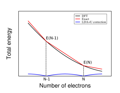
Figure 5: (Color online) Sketch of the total energy profile as a function of the number of electrons in a generic atomic system in contact with a reservoir. The black line represents the DFT energy, the red the exact limit, the blue the difference between the two. The discontinuity in the slope of the red line for integer occupations, corresponds to the difference between ionization potential and electron affinity and thus measures the fundamental gap of the system.

If the curvature of the approximate energy profile is assumed to be constant (actually a very good approximation within single intervals between integer occupations dabo10 ), the expression of the additive correction needed to recover the exact behavior (bottom line in the cartoon of Fig. 5) can be easily worked out as the difference between a parabola and a straight line and results to have the same expression of the Hubbard correction in Eq. (13), provided the $U$ is equal to the (spurious) curvature of the DFT energy profile. Therefore, the main objective of this calculation is to evaluate the second derivative of the total energy of the system with respect to the occupation of the localized states, as defined in Eq. 3.

In codes that are not based on localized basis sets, (and use, e.g., plane waves and pseudopotentials) the on-site occupations are obtained as an outcome from the calculation after projecting Kohn-Sham states on the wave functions of the localized basis set (Eq. (3)). Therefore, to compute the second derivative of the total energy with respect to the occupations, a different approach was adopted that is based on Legendre transforms cococcioni05 . The first step consists in applying a shift to the external potential that only acts on the localized orbitals of a Hubbard atom $I$ through a projection operator:

$$v^{p}_{ext}=v_{ext}+\alpha^{I}\sum_{m}|\phi_{m}^{I}\rangle\langle\phi_{m}^{I}|$$ (22)

(the superscript “p” standing for “perturbed”). In this equation $\alpha^{I}$ represents the amplitude of the perturbation (usually chosen small enough to maintain a linear response regime). The potential in Eq. (22) is the one used to solve the KS equations. They yield a $\alpha$-dependent ground state charge density and total energy:

$$E(\alpha^{I}) = \sum_{i,\sigma}\epsilon_{i}^{\sigma}(\alpha^{I})-\frac{1}{2}\int v_{H}[\rho_{\alpha^{I}}({\rm\bf r})]\rho_{\alpha^{I}}({\rm\bf r})d{\rm\bf r}$$ (23)

$$+ E_{xc}[\rho_{\alpha^{I}}]-\int v_{xc}[\rho_{\alpha^{I}}({\rm\bf r})]\rho_{\alpha^{I}}({\rm\bf r})d{\rm\bf r}$$

where $\epsilon_{i}^{\sigma}(\alpha^{I})$ are the single-particle energies obtained from the solution of the KS problem. An occupation-dependent total energy functional can be recovered from the expression in Eq. (23) using a Legendre transform: $E[\{n^{I}\}]=E(\alpha^{I})-\alpha^{I}n^{I}$ (where $n^{I}$ indicates the value of the on-site occupation corresponding to the perturbed ground state). Based on this definition, the first and second derivatives of the energy are, respectively,

$$\frac{dE}{d(n^{I})}=-\alpha^{I}$$ (24)

and

$$\frac{d^{2}E}{d(n^{I})^{2}}=-\frac{d\alpha^{I}}{d(n^{I})}.$$ (25)

In actual calculations the latter quantity is obtained by solving the Kohn-Sham equations for a range of values of the parameter $\alpha^{I}$ (on every Hubbard atom) centered around 0 and collecting the response of the system in terms of the variation of the total occupations $n^{J}$ of all the atoms. The operation is repeated perturbing each Hubbard atom separately. The quantity that can be directly measured from this series of calculations is the response matrix

$$\chi_{IJ}=\frac{d(n^{I})}{d\alpha^{J}},$$ (26)

where $I$ and $J$ are site indices that label the Hubbard atoms. The curvature of the total energy (Eq. 25) with respect to the occupations $n^{I}$ is thus obtained as the inverse of the response matrix: $d^{2}E/d(n^{I})^{2}=-(\chi^{-1})_{II}$. This quantity is not the effective $U$. In fact, applying a perturbation as the one in Eq. (22) to a non interacting electron system, also results in a response of the occupations (due to the rehybridization of the electronic wave functions) that contributes a finite term to the second derivative of the total energy. Based on Eq. (25) and on the definition of the response matrices, this “non-interacting” contribution can be expressed as $d^{2}E/d(n^{I})_{0}^{2}=-(\chi_{0}^{-1})_{II}$, $d(n^{I})_{0}$ being the variation of occupation due to the above mentioned rehybridization. Being not related to electron-electron interactions, this term should be subtracted from the second derivative of the total energy. The Hubbard $U$ is thus obtained as:

$$U^{I}=(\chi_{0}^{-1}-\chi^{-1})_{II}.$$ (27)

As the response of a non interacting electron gas (with the same density of the interacting one), $\chi_{0}^{-1}$ is sometimes interpreted as the kinetic (or single-body) contribution to the second derivative of the energy pickett98 . In order to understand how $\chi_{0}$ is actually computed, it is useful to realize that it measures the response of the system to a variation of the total potential (while $\chi$ is the response to the variation to the external potential). In other words:

$$\Delta n^{I}=(\chi_{0})_{IJ}\Delta V^{tot}_{J}=\chi_{IJ}\Delta V^{ext}_{J}=\chi_{IJ}\Delta\alpha^{J}.$$ (28)

The calculation of $\chi_{0}$ requires special care in the iterative solution of the Kohn-Sham equations at finite $\alpha^{I}$. In fact, $\chi_{0}$ is calculated from the variation of the atomic occupations immediately after the first diagonalization of the Hamiltonian resulting from the sum of the self-consistent (unperturbed) KS Hamiltonian and the perturbative potential in Eq. (22). At this initial step of the perturbed run, the variation of the external potential has not yet been screened by the response of the electronic charge density (through the Hartree and xc potentials) and is thus coincident with the variation of the total potential: $\Delta V^{tot}_{J}=\Delta V^{ext}_{J}=\Delta\alpha_{J}$. Thus, from Eq. (28), one easily obtains: $(\chi_{0})_{IJ}=(\Delta n^{I}/\Delta\alpha^{J})_{first}$. Therefore, the first diagonalization of the electronic Hamiltonian in the perturbed run must be very precise in order to obtain an accurate non-interacting response matrix $\chi_{0}$. $\chi$ is instead computed after the perturbed calculation has reached self-consistency: $\chi_{IJ}=(\Delta n^{I}/\Delta\alpha^{J})_{last}$.

It is important to stress that the linear-response calculations to compute the response matrices $\chi$ and $\chi_{0}$ are performed in a supercell of the crystal (whose size is determined from the convergence of the obtained Hubbard $U$ cococcioni05 ) where only one atom is perturbed each time. In fact, consistently with the treatment of localized states as isolated atomic orbitals in contact with a bath (represented by the rest of the crystal), and with the definition of the Hubbard $U$ as the energy cost associated with the double occupancy of the orbitals of a single atom, it is necessary to isolate the atom with perturbed states and to avoid the interaction with its periodic images. If the separation between perturbed atoms (i.e., the size of the supercell) is not large enough, the resulting $U$ is screened, to some extent, by the residual coupling between the perturbations on equivalent atoms and, when used in LDA+U calculations (in the actual unit cell of the crystal), it incurs in some double screening. The charge redistribution induced by the perturbation in the external potential, Eq. (22), usually involves multiple Hubbard atoms. This is the reason for which $U$ is obtained from inverting the entire response matrices rather than their single (diagonal) elements. In Ref. cococcioni05 the matrices $\chi$ and $\chi_{0}$ are constrained to represent the response of a system to a neutral perturbation. This amounts to impose the sum of the matrix elements on the same row and the same column to be zero by adding a neutralizing “background” (described by an extra row and an extra column in each of these matrices). However this condition would be legitimate to impose only if there was a perfect overlap between the Hilbert spaces spanned by atomic and KS states (never exactly the case, in practice). Recently, it was realized that a better way to account for the charge reservoir Hubbard atom exchange electrons with, while screening the external perturbation, is to explicitly include in $\chi$ and $\chi_{0}$ the collective response of “non Hubbard” atoms and states (also collected in an extra row and an extra column) and to also consider the response of the system to their collective perturbation (obtained from imposing the same $\alpha$ to all these states at the same time). This refinement was found to have beneficial effects on the convergence of the calculation with the size of the chosen supercell.

Following the same procedure illustrated above for the Hubbard $U$, the intra-atomic exchange interaction $J$ could, in principle, be obtained in a similar way, adding a perturbation that couples with the on-site magnetization $m^{I}=n^{I\uparrow}-n^{I\downarrow}$:

$$v^{p}_{ext}=v_{ext}+\beta^{I}\sum_{m}\left[|\phi_{m}^{I\uparrow}\rangle\langle\phi_{m}^{I\uparrow}|-|\phi_{m}^{I\downarrow}\rangle\langle\phi_{m}^{I\downarrow}|\right].$$ (29)

However, since the total energy is not variational with respect to the magnetization, and the magnetization of a system often reaches its saturation value (compatibly with the number of electronic states), a perturbative approach is generally not viable. Also, in these circumstances, $n^{I}$ and $m^{I}$ are not independent variables (in fact, only one spin population can be perturbed, the other spin states being fully occupied and typically removed from the Fermi level) and only linear combinations of $U$ and $J$ can be obtained from LR, not their separate values. A possible way around this problem consists in perturbing a ground state whose absolute magnetization has been constrained to be lower than its saturation value so that $n^{I}$ and $m^{I}$ can be varied independently. However, calculations of this kind require effective constraints on the atomic magnetization of atoms and turn out to be technically difficult to perform and very delicate to bring to convergence.

Similar problems arise when computing $U$ for fully occupied or empty states. In fact, the linear-response approach discussed above is suitable to calculate the effective electronic coupling of manifolds of states that are either in the vicinity of the Fermi level (and thus partially full), or result from the hibridization of atomic orbitals of different atoms (as, e.g., the valence states in bulk elemental semiconductors). If the manifold is completely full (e.g., the O $p$ states in some transition metal oxides) and distant in energy from the Fermi level or the top of the valence band, their response is very small and may easily fall within the numerical noise of the calculation. In these cases the reliability of the obtained $U$ is questionable (values of 30 eV or higher are not uncommon). Whether or not a preliminary shift of the manifold closer to the Fermi level could be a solution, depends on the specific material and on the entity of the collateral effects this shift has on its electronic structure and its physical properties.

III.3.2 The analytic expression of $U$ and the problem of screening

It is useful, at this point, to study the analytic expression of the Hubbard $U$, obtained, as detailed in appendix A, from the (linear) response of atomic occupations to a perturbation in the potential acting on localized orbitals that is a generalization of the one given in Eq. (22). If the definition of the occupation matrix is extended to contain off-diagonal terms with atomic orbitals belonging to different sites $I$ and $J$, $n^{IJ}_{i,j}=\sum_{n}f_{n}\langle\psi_{n}|\phi_{j}^{J}\rangle\langle\phi_{i}^{I}|\psi_{n}\rangle$ (this extension will be also needed for the LDA+U+V functional, discussed in section VI.1), and the perturbation to the external potential is generalized accordingly to $\Delta V_{ext}^{LM}=\alpha^{LM}_{lm}|\phi^{L}_{l}\rangle\langle\phi^{M}_{m}|$ a four-index response matrix can be defined as follows:

$$\tilde{\chi}^{JKML}_{jkml}=\frac{dn^{JK}_{jk}}{d\alpha^{LM}_{lm}}$$ (30)

where upper case letters indicate atomic sites, lower case letters label atomic states.

The matrix $\tilde{\rm\bf U}$, that is obtained from the inversion of this matrix (and its non-interacting analog $(\tilde{\chi}_{0})^{JKML}_{jkml}$), as indicated in Eq. (27), consists of the expectation values of the Hartree and exchange-correlation interaction kernels over the states of the atomic basis set:

$$\tilde{U}^{OPSR}_{opsr}=(\tilde{\chi}_{0}^{-1}-\tilde{\chi}^{-1})^{OPSR}_{opsr}=$$

$$\int\int(\phi^{O}_{o}({\rm\bf r}))^{*}\phi_{p}^{P}({\rm\bf r})f_{Hxc}({\rm\bf r},{\rm\bf r}^{\prime})\phi^{S}_{s}({\rm\bf r}^{\prime})^{*}\phi^{R}_{r}({\rm\bf r}^{\prime})~{}d{\rm\bf r}~{}d{\rm\bf r}^{\prime}.$$ (31)

This expression might surprise for the lack of screening. A similar result was obtained in Ref. anisimov07 where the definition of an orbital dependent functional, able to eliminate the spurious curvature of the DFT energy and to re-establish the finite discontinuity of the potential, was based on the same unscreened interaction kernel as the one in Eq. (III.3.2). The specialization of this correction to a fixed basis set of Wannier functions also resulted in a final expression resembling closely the LDA+U one with effective interactions computed as in Eq. (III.3.2). It is important to remark that the Hubbard $U$ used in actual LDA+U calculations is not the one given in Eq. (III.3.2) but, rather, the one calculated as in Eq. (27), which is based on the response matrices measuring the variation of the total on-site occupations $n^{I}$ (Eq. (26)) in response to (diagonal) perturbations acting on all the states of each atom. While linear response equations do not have a closed form for the two-atomic-indexes response matrices, the following formal relationship can be derived (appendix A) between the effective Hubbard $U$ and the one in Eq. (III.3.2):

$${\rm\bf U}=({\rm\bf\chi_{0}})^{-1}{\rm\bf A}~{}{\rm\bf\chi}^{-1}.$$ (32)

where the response matrix, defined in Eq. (26), can be obtained from the contraction of its four indices analog in Eq. (30): $\chi^{IR}=\sum_{ir}\tilde{\chi}^{IIRR}_{iirr}$ and the matrix A is defined as follows:

$$A^{RS}=\sum_{rs}\sum_{KQTZ}\sum_{kqtz}\left(\tilde{\chi}_{0}\right)^{RRQK}_{rrqk}\tilde{U}^{KQTZ}_{kqtz}\tilde{\chi}^{ZTSS}_{ztss}$$ (33)

(refer to Eq. (88) for the expression of U in terms of $\tilde{\rm\bf U}$ with explicit sums over state and site indexes). It is instructive, at this point, to compare the effective $U$ obtained from the linear-response (LR) method outlined above, Eq. (89), with the one computed from cRPAarya04 (neglecting the frequency dependence of the dielectric constant), Eq. (21). The difference between the two results is in the way the screening is performed. If all the electronic states were treated explicitly, a bare (i.e., unscreened) interaction (Eq. (III.3.2)) is obtained with both methods. This case has been discussed in appendix A for LR, and would correspond to putting $\epsilon=\epsilon_{d}$ (i.e., $\epsilon_{r}=1$) in the cRPA method. As described earlier, within cRPA the (kernel of the) effective interaction is computed as $\epsilon_{r}^{-1}f_{Hxc}$, through the screening operated by all the electronic degrees of freedom not treated explicitly in the model Hamiltonian (e.g., by $d-s$ or $s-s$ transitions, $s$ indicating non Hubbard states). An analogous approach in LR would require writing $\epsilon^{-1}=\chi_{0}^{-1}\chi$ as the product of two contributions, from localized ($d$) and delocalized ($s$) states or, equivalently, to write $\chi_{0}$ as the sum of $d$ and $s$ terms, $\chi_{0}=\chi_{0}^{d}+\chi_{0}^{s}$. However, this is not possible, due to the “coarse-grained” nature of the response matrices employed. In LR an effective screening of the electronic interaction is operated by the matrix multiplications in Eq. (33) that contain summations over transitions between $d$ states of distinct atomic sites, between $d$ and $s$, and between $s$ and $s$ states. These summations lead to a significant contraction of the computed interactions whose value decreases from 15-30 eV, typical of the unscreened quantitity, to the 2-6 eV range of the effective one. A qualitative argument to understand this result is as follows: when an electron (or a fraction of it) is moved on to a specific atomic site and increases its occupation, it is drawn from other states and orbitals, resulting in negative state- and site-off-diagonal elements of the response matrices in the multiplication of Eq. (33). In other words, the effective energy cost of double occupancy of the considered site is reduced by the decreased weight of other terms of the electron-electron interaction, mostly involving off-diagonal terms of the occupation matrices. From these observations, further detailed at the end of appendix A, we can conclude that the effective $U$ obtained from LR can be best understood as resulting from the downfolding of the electron-electron interaction to the $d$ (localized) states, after the elimination of higher order off-diagonal $d-d$, $d-s$ and $s-s$ transitions.

III.3.3 Ab-initio LDA+U: examples

The calculation of the effective Hubbard $U$, described above, renders the LDA+U an ab initio method, eliminating any need of semi-empirical evaluations of the interaction parameters in the corrective functional. It also introduces the possibility to compute the values of these interactions in consistency with the choice of the localized basis set, the crystal structure, the magnetic phase, the crystallographic position of atoms, etc. This ability proved critical to improve the predictive capability of LDA+U and the agreement of its results with available experimental data for a broad range of different materials and conditions. The capability to compute the interaction parameters significantly improves the description of the structural, electronic and magnetic properties of a variety of transition-metal-containing crystals and was particularly useful in presence of structural transformations cococcioni05 ; hsu09 , magnetic transitions hsu11 and chemical reactions zhou04-1 ; zhou04-2 . In Ref. hsu11 the use of a Hubbard $U$ recomputed for different spin configurations allowed to predict a ground state for the (Mg,Fe)(Si,Fe)O₃ perovskite with high-spin Fe atoms on both A and B sites, and a pressure-induced spin-state crossover of B-site Fe atoms that couples with a significant volume contraction, an increase in the quadrupole splitting (consistent with recent X-ray diffraction and Mössbauer spectroscopy measurements) and a marked anomaly in the bulk modulus of the material under pressure. The calculation of the Hubbard $U$ also improved the energetics of chemical reactions kulik06 ; scherlis07 , and electron-transfer processes sit06 . A recent extension to the linear response approach has further increased its reliability through the self-consistent calculation of the $U$ from an LDA+U ground state campo10 ; kulik06 . This method is mostly useful for systems where the LDA and LDA+U ground states are qualitatively different. It is based on a similar calculation to the one described above except that the perturbative LDA+U calculation is performed with the Hubbard corrective potential frozen to its self-consistent unperturbed value. This strategy guarantees that the “+U” part does not contribute to the response of the system and, consistently to its definition, the Hubbard $U$ is measured as the curvature of the LDA energy in correspondance of the LDA+U ground state. Using the Hubbard $U$ computed at the previous step to induce the LDA+U ground state for the next, the calculation is repeated cyclically until when the input and otput values are numerically consistent. The procedure usually reaches convergence in few cycles (less than five in most cases). Recently a similar self-consistent calculation of $U$ has been also implemented for the cRPA approach karlsson10 .

IV Choosing the localized basis set

The choice of the localized basis set to define the occupation matrix and the possible dependence of the results on this choice remain open issues of the LDA+U method. Very often this choice is dictated by the specific implementation of DFT being used (e.g., based on gaussian functions, muffin-tin orbitals and augmented plane waves, etc). In principle, if the localized basis set were $i)$ orthonormal and $ii)$ complete, $iii)$ the effective interactions had full orbital dependence, and $iv)$ their numerical value was chosen/computed consistently with the basis set, the results obtained from LDA+U calculations would not depend on the choice of the basis set. Since, in practice, the first three conditions (and often the forth too) are never verified, some care must be used in the selection of the localized orbitals. In fact, when basis sets are finite, switching from one to another only generates an equivalent description if the two span the same Hilbert space. Consistently with our plane wave, pseudopotential implementation of LDA+U giannozzi09 , in this section we will only discuss basis sets consisting of atomic orbitals (e.g., from the pseudo potentials) or Wannier functions.

The choice of atomic orbitals (e.g., solutions of the radial Schrödinger equation for isolated atoms, multiplied by spherical harmonics) is somewhat “natural” to LDA+U since it is based on the Hubbard model that was designed to capture the Mott localization of electrons on atoms. In addition, in its simplest version, it contains only “on-site” interaction parameters accounting for the Coulomb repulsion betwen electrons on the same atom. However, as discussed in section II.4, the Hubbard functional can be associated to a broader scope and it can be regarded as a simple correction designed to impose to the exchange correlation potential the discontinuity it is supposed to have (the Hubbard $U$ is actually the amplitude of the discontinuity) and to obtain a Kohn-Sham HOMO-LUMO gap equal to the fundamental gap of the considered system. In its original formulation, it is most effective when the gap is to result from lifting the (nearly exact) degeneracy of localized atomic states (typically $d$ or $f$) of open-shell systems. The localized character of these states is indeed what justifies orbital-, k-point-independent and (usually) atomically averaged effective interactions. This approximation remains indeed well justified even for systems where electronic localization occur on more general orbitals (centered, for example, on bonds). In these cases, however, the correction loses its atomic character and the effective interactions should be recomputed accordingly.

IV.1 Atomic orbitals

Atomic orbitals are usually obtained from the solution of the radial Schrödinger equation for isolated atoms (the angular part is added when performing calculations for the systems of interest). These orbitals are represented by wave functions centered on the single atoms and decaying with the distance from its nucleus: $\phi_{m}^{IR}=\phi_{m}({\rm\bf r}-{\rm\bf\tau_{I}}-{\rm\bf R})$. In this expression ${\rm\bf\tau_{I}}$ is the position of the $I^{th}$ atom in each unit cell of the crystal (or in the molecule), ${\rm\bf R}$ designates the unit cell. The atomic orbital occupations, Eq. 3, should be defined, in principle, by specifying the unit cell the atomic wave function is localized in. However, the periodicity of the crystal allows us to drop this index from the expression of the occupation matrices and to use the definition in Eq. (3). Consequently, the Hubbard energy (per unit cell) does not depend on ${\rm\bf R}$ and can be computed from a single unit cell. The expression in Eq. (13) can be understood as obtained from the unit cell at ${\rm\bf R}={\bf 0}$: $\frac{1}{N}\sum_{{\rm\bf R}I}\frac{U^{I}}{2}Tr\left[{\bf\rm n}^{{\rm\bf R}I\sigma}\left(1-{\bf\rm n}^{{\rm\bf R}I\sigma}\right)\right]=\sum_{I}\frac{U^{I}}{2}Tr\left[{\bf\rm n}^{{\rm\bf 0}I\sigma}\left(1-{\bf\rm n}^{{\rm\bf 0}I\sigma}\right)\right]=\sum_{I}\frac{U^{I}}{2}Tr\left[{\bf\rm n}^{I\sigma}\left(1-{\bf\rm n}^{I\sigma}\right)\right]$. It is important to stress that the projection of the atomic wave function on a Kohn-Sham state at a given k-vector ${\rm\bf k}$ selects the Fourier component of the localized atomic orbital at the same k-vector (and at all the ${\rm\bf k+G}$ points, ${\rm\bf G}$ being a fundamental vector of the reciprocal lattice). Therefore, the calculation of atomic occupations in Eq. 3 would give exactly the same result if, instead of localized atomic orbitals, their Bloch sums were used. This observation will be important when computing the derivatives of the occupation matrices to obtain, for example, forces and stresses (see section VII).

A problem that arises with atomic wave functions is the finite overlap between orbitals belonging to neighbor atoms. This fact compromises the summation rules of atomic occupations in Eq. 3 (some portion of electrons are counted more than once) and make the Hubbard energy and potential less well defined (some occupations may exceed 1). The problem can be solved performing a preliminary orthogonalization of the atomic basis set using, for example, Löwdin decomposition. Within this scheme an orthonormal basis set can be obtained as

$$\phi_{i}^{orth}=\sum_{j}O^{-1/2}_{ij}\phi_{j}$$ (34)

where $O_{ij}=\langle\phi_{i}|\phi_{j}\rangle$ is the overlap matrix between orbitals of the original basis set (the low case indexes $i$ and $j$ are comprehensive of site and state labels). The mixing of orbitals from different sites through the overlap matrix in Eq. 34 leads to a loss of the atomic character of the wave functions; however, the contribution from neighbor sites is usually small and their use in a Hubbard-modeled correction with atomic interactions is still largely legitimate.

It is important to stress that the use of an orthogonalized basis set makes the calculation of energy derivatives significantly more challenging. In fact, the overlap matrix in Eq. (34) does not usually commute with its derivative (nor do its powers, obviously) so that the derivative of ${\rm\bf O}^{-1/2}$ can not be easily obtained from that of ${\rm\bf O}$ (a numerical solution to this problem could be obtained exploiting the fact that ${\rm\bf O}$ should contain a relatively small deviation from the unit matrix ${\rm\bf O}=({\rm\bf 1}+{\rm\bf t})$ and a series expansion on ${\rm\bf t}$ should converge rapidly). As a consequence, when derivatives of the energy are needed, a non-orthogonal basis set is generally used.

It is also useful to keep in mind that the effective interaction parameter to be used in the Hubbard functional is sensitive to the specific localized basis set used to define the atomic occupations and the difference between orthogonalized and non-orthogonalized wave functions is sufficient to cause an appreciable variation in its value. Therefore, the Hubbard $U$ should be recomputed consistently e.g., using the linear response technique discussed in section III, with the same basis set employed in the costruction of the functional.

Another possible way to eliminate or significantly alleviate the orthogonalization problem consists in truncating the atomic wave function at the core radius of the pseudopotential of the atoms they belong to. In this way, the integration of on site occupations is restricted within the regions around the atomic cores and the Hubbard potential amounts to a renormalization of the coefficients $D^{I}_{ij}$ of the non-local pseudopotential:

$$V_{tot} = V_{loc}+V_{NL}+V_{Hub}$$ (35)

$$= V_{loc}+\sum_{I}\sum_{ij}\left(D^{I}_{ij}+\Delta^{I}_{ij}\right)|\beta_{i}^{I}\rangle\langle\beta^{I}_{j}|.$$

In this expression $\Delta^{I}_{ij}$ contains the expectation value of the Hubbard potential on the all-electron partial waves of the pseudopotential, corresponding to the projector waves $\beta^{I}_{i}$. While Eq. (35) uses a formalism that resembles that of ultrasoft pseudopotentials vanderbilt90 , it can be used with general non-local pseudopotentials. This implementation of the Hubbard functional was first introduced in a projector-augmented wave framework in Ref. bengone00 where it was also shown that the charge excluded from the atomic cutoff spheres is usually small and contributes negligible corrections to the Hubbard functional. In Ref. sclauzero13 this pseudopotential implementation of LDA+U was adapted to general non-local pseudopotentials and used to study the ballistic electron transport in Au monoatomic chains. A similar method was also used to construct an atomic self-interaction correction and to effectively embed it in the pseudopotential filippetti03 ; filippetti03_1 ; sanvito07 ; filippetti09 .

IV.2 Wannier functions

If electrons localize on states that are not centered on atoms, a Hubbard corrective functional based on atomic states and on-site only interactions is not likely to improve the description of the corresponding ground state. A possible solution to this problem consists in generalizing the expression of the Hubbard corrective functional to include interaction terms (e.g., between electrons on different atoms) that are usually neglected in the on-site formulations and to partially recover the invariant second-quantization expression of the Hubbard functional hubbardI ; hubbardII ; hubbardIII ; hubbardIV ; hubbardV ; hubbardVI with orbital- and/or site-dependent effective electronic interactions. This approach is the one followed in the formulation of the LDA+U+V correction that, through including inter-site interactions, proves able to capture the localization of electrons on the $sp^{3}$ bonds of covalent semiconductors (e.g., Si). This generalization is presented in section VI.1 and won’t be further discussed here.

An alternative approach to this problem consists in adopting a basis set of orbitals particularly suitable to capture the localization of electrons in the considered system. In the case of elemental band semiconductor (e.g., Si) this would imply to use, for example, Wannier functions centered around the Si-Si bonds. While this choice of basis functions guarantees the possibility to still use a “localization-center-diagonal” interaction term, it requires a preliminary knowledge about the localization centers of the electrons or an additional mathematical criterion (e.g., maximal localization marzari97 ) to precisely define the basis set. Wannier functions have indeed become a quite popular choice in recent years to define corrective functionals and computational schemes to improve the description of electronic localization in strongly correated systems. In Refs lechermann06 ; trimarchi08 , for example, maximally-localized Wannier functions (MLWF) marzari97 were used to facilitate the identification of correlated orbitals and to construct a more flexible and general interface between DFT and DMFT that allows to construct a DFT+DMFT scheme from all possible implementations of DFT as, for example, those based on plane waves and psudopotentials. In Ref. anisimov07 Wannier functions were instead employed to construct a LDA+U - like correction to the DFT total energy aimed at restoring the discontinuity in the exchange-correlation potential, generally missing in approximate functionals. While MLWF are a popular choice for the definition of many of these functionals based on Wannier functions, other schemes have also been employed in literature.

In Refs. oregan10 ; oregan11 ; oregan12 non-orthogonal generalized Wannier functions (NGWF) were used to define a LDA+U scheme compatible with linear-order-scaling ($O(N)$) DFT. Within this implementation, based on a generalized covariant-controvariant definition of the occupation matrix, the total energy is minimized with respect to both the kernel of the density matrix and with respect to the coefficients of the expansion of the NGWF on the Kohn-Sham states. This “internal” minimization, while adding a negligible overload to the calculation, leads to a variational optimization of the localized basis set used in the definition of the Hubbard correction. The WF basis obtained in this way thus results optimally adapted to capture electronic localization and to produce a density matrix as close as possible to be idempotent.

An alternative WF-based LDA+U approach was proposed in Refs fabris05 and fabris05_1 where the Wannier functions were defined (from the Kohn-Sham states of the system) by maximizing their overlap with the atomic wave functions of “Hubbard” atoms. This LDA+U scheme was used to study the electronic structure around an oxygen vacancy on the surface of CeO₂, a material often employed in the catalytic purification of exhaust gases resulting from various processes. It was found that LDA+U (with the Hubbard interaction computed from linear responsecococcioni05 ) favors the reduction of two of the Ce atoms around the oxygen vacancy (first neighbors) from 4+ to 3+, inducing the localization of the two excess electrons on their $f$ states. This redistribution of charge is indeed in better agreement with experiments and chemical intuition than a metallic state with excess elecrons spread among the $f$ orbitals of all the Ce atoms surrounding the vacancy, as predicted by non corrected DFT functionals. More importantly, it was found that the Wannier function-based LDA+U scheme works better, in this case, than one using occupations defined on atomic orbitals. In fact, because of the optimal overlap with the atomic states of “Hubbard” atoms, the use of Wannier functions allowed to effectively separate the fully occupied (valence) manifold from the empty (conduction) one. With all the occupations equal to either 0 or 1, the total energy of the system does not depend on the value of the Hubbard $U$, as it can be easily understood from Eq. (13), and the agreement of the computed reduction energy with availale experiments was significantly improved. It is important to notice that the effective interaction $U$ still controls the position of the Hubbard bands (the Ce $f$ states in this case) with respect to the conduction and valence manifolds. In fact, the Hubbard potential (Eq. (4)) does not vanish in this case and rigidly shifts the energy of the unoccupied states with respect to that of unoccupied ones. Therefore, even in cases where the energy does not depend on $U$, its calculation is still important to accurately describe the electronic properties of the system and its chemical reactivity.

V The double-counting “issue” and the LDA+U for metals

V.1 Comparison between the FLL and the AMF approaches

The choice of the double counting term certainly represents an open issue of the LDA+U method. The lack of an explicit expression of the xc energy makes it difficult to model how electronic correlation is accounted for in approximate DFT energy functionals. As a result, simple dc functionals, like the ones in Eqs. (II.2) and (13), are not general and flexible enough to work equally well for all kinds of systems.

In section II and III it was shown how the “fully-localized” (FLL) formulation of the LDA+U is constructed to impose a finite discontinuity to the xc potential. Since this discontinuity also represents an important term of the fundamental gap of a system, it is natural to expect that this specific formulation is particularly effective to improve the description of semiconductors and insulators, but not well suited to treat metals or “weakly correlated” materials in general. In fact, the eccessive stabilization of occupied states due to the “+U” corrective potential (see Eq. 4) can lead to a description of the ground state inconsistent with experimental data and to quite unphysical results (such as, e.g., the enhancement of the Stoner factor chioncel03 ) or serious discrepancies with available experimental evidence (e.g., in the equilibrium lattice parameter or in the bulk modulus cococcioni05 ) that seriously question its applicability in these cases.

The “around mean-field” (AMF) formulation of LDA+U was introduced to alleviate these difficulties and to improve the description of correlation in systems where electronic localization is less pronounced or for which a metallic behavior is expected. The AMF LDA+U was actually the first one to be introduced anisimov91_2 and in its simplest formulation the energy functional can be expressed as follows:

$$E_{LDA+AMF}=E_{LDA}$$

$$+\frac{1}{2}\sum_{mm^{\prime}\sigma}U(n_{m\sigma}-\langle n\rangle)(n_{m^{\prime}-\sigma}-\langle n\rangle)$$

$$+\frac{1}{2}\sum_{mm^{\prime}\sigma}^{*}(U-J)(n_{m\sigma}-\langle n\rangle)(n_{m^{\prime}\sigma}-\langle n\rangle)$$ (36)

where the asterisk on the second summation indicates it runs over all the $m$ and $m^{\prime}$ such that $m\neq m^{\prime}$ and $\langle n\rangle=\frac{1}{2(2l+1)}\sum_{m\sigma}n_{m\sigma}$. The idea that inspired this formulation is quite different from the one behind the FLL atomic limit czyzyk94 . While the latter can be viewed as introducing a finite energy cost for occupations of localized orbitals deviating from integer values, the AMF corrective functional can be regarded as a penalty against deviations (fluctuations) of the occupations from their mean value. This latter approach corresponds to considering the approximate DFT total energy as containing a mean field approximation of the electron-electron interaction. This is easily seen from the identity czyzyk94 : $n_{m\uparrow}n_{m^{\prime}\downarrow}=n_{m\uparrow}\langle n_{\downarrow}\rangle+\langle n_{\uparrow}\rangle n_{m^{\prime}\downarrow}-\langle n_{\uparrow}\rangle\langle n_{\downarrow}\rangle+(n_{m\uparrow}-\langle n_{m\uparrow}\rangle)(n_{m\downarrow}-\langle n_{m\downarrow}\rangle)$. It is evident that, if the LDA (or any approximate) xc functional contains the first three terms on the rhs of this expression (the mean-field approximation of the quantity on the lhs), the AMF correction, proportional to the last term on the rhs (Eq. (V.1)) is exactly what is needed to recover the product of occupation matrices from its mean field value.

To better understand the differences between the FLL and the AMF formulations of LDA+U it is convenient to follow Ref. czyzyk94 and to rewrite both functionals in the form:

$$E_{LDA+U}=E_{LDA}+H_{Hub}-\langle H_{Hub}\rangle.$$ (37)

In both flavors, $H_{Hub}$ contains electron-electron interactions as modeled in the Hubbard Hamiltonian:

$$H_{Hub} = \frac{1}{2}\sum_{mm^{\prime}\sigma}Un_{m\sigma}n_{m^{\prime}-\sigma}$$ (38)

$$+ \frac{1}{2}\sum_{mm^{\prime}\sigma}^{*}(U-J)n_{m\sigma}n_{m^{\prime}\sigma}$$

(rotational invariance is neglected here) where the asterisk has the same meaning as in Eq. (V.1). The difference between the FLL and the AMF formulations thus amounts to a different dc term $\langle H_{Hub}\rangle$. In fact, one can recover the two corrective functionals using, in Eq. (37), the following two expressions for $\langle H_{Hub}\rangle$ czyzyk94 :

$$\langle H_{Hub}\rangle_{AMF}=UN_{\uparrow}N_{\downarrow}+\frac{1}{2}(U-J)\frac{2l}{2l+1}(N_{\uparrow}^{2}+N_{\downarrow}^{2})$$

$$\langle H_{Hub}\rangle_{FLL}=\frac{U}{2}N(N-1)-\frac{J}{2}\sum_{\sigma}N_{\sigma}(N_{\sigma}-1)$$ (39)

where $N_{\sigma}=\sum_{m}n_{m\sigma}$ and $N=N_{\uparrow}+N_{\downarrow}$. A comparative analysis of these dc terms (in particular, their like-spin parts) highlights the different “philosophy” behind them: while in the AMF every electron interacts with all the electrons in the system (suggesting a spread charge density) and the self-interaction is eliminated through the rescaling (by a factor $\frac{2l}{2l+1}$) of the effective interaction parameter, in the FLL limit, due to a more pronounced localization, each electron interacts with the other N-1. An exhaustive discussion about the main ideas at the basis of both the FLL and the AMF formulations, their theoretical framework within density functional theory, and their specific characteristics, has been also presented in Ref. anisimov07 . A comparison between these two flavors was also offered in Ref. eschrig2003 .

An attempt to obtain a general correction that bridges the AMF and the FLL formulations and is able to treat a broad range of systems with intermediate degrees of electronic localization has been made in Ref. chioncel03 . This work proposes a linear combination of the AMF and the FLL flavors of LDA+U, based on a mixing parameter that has to be determined for each material and is a function of various quantities related to its electronic structure. This approach has been used to study intermetallic chioncel03 and selected rare earth compounds bultmark09 showing promising results and a significant improvement with respect to either functional. In spite of the desirable capability to improve the prediction of properties related to electronic localization (such as, e.g., magnetization) without compromising the description of delocalized electrons, this approach, as well as the AMF itself, has had limited popularity due, perhaps, to the diffusion of DFT+DMFT. In fact, this scheme offers a more rigorous treatment of dynamical effects (particularly important for metallic system) and is able to capture, within the same theoretical framework, the physics of systems and phases characterized by widely different levels of electronic localization. At the same time the LDA+U method has been identified almost exclusively with its FLL limit (because of a closer adherence to the formulation of the Hubbard model) and has been mostly used for systems with strongly localized electrons where the main consequence of (static) electronic correlation usually consists of the onset of an insulating ground state.

Is the FLL formulation only suitable for re-establishing the discontinuity of the xc potential and inserting it in the Kohn-Sham spectrum of a system? In view of its ability to increase the separation in energy between full and empty states, the FLL corrective functional could still be useful to selectively correct the energetics of localized states (i.e., the position of the corresponding bands) while leaving more itinerant ones, or those in the vicinity of the Fermi level uncorrected. In bulk transition metals (generally cubic and often magnetic), for example, it was recognized that the $e_{g}$ subgroup of the $d$ orbitals form bands significantly more localized than the t_2g ones goodenough60 . Consistently with this observation, the use of the FLL “+U” functional to correct only the $e_{g}$ $d$ states of bulk Fe, has shown a significant improvement in the prediction of the equilibrium lattice parameter and of the bulk modulus of the material with respect to LDA+U calculations with the Hubbard functional applied to all the $d$ states. Similar results have also been obtained for a variety of metallic systems leonov11 ; himmetoglu12_1 with an analogous correction on localized $d$ states.

As another example, figure 6 shows the band structure and the density of states of PbCrO₃ and compares GGA (PBE) results (top panel) with GGA+U (bottom panel). The transitions this material undergoes between antiferromagnetic (AFM), ferromagnetic (FM), and canted orders have not yet been completely clarified (see Refs. roth67 ; arevalo08 ; arevalo09 and references quoted therein). The calculations whose results are shown in Fig. 6 (performed within the AFLOW framework curta12 ; curta12_1 ; curta12_2 ) assumed a ferromagnetic ground state.

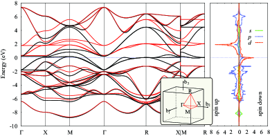
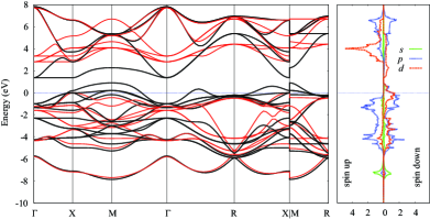
Figure 6: (Obtained from kyang13 , color online) Electronic band structure (left) and density of states (right) of PbCrO₃. The high symmetry Brillouin zone path used for the electronic band structure calculation is shown in the inset. The upper panel shows PBE results, the lower ones, PBE+U. Red lines are for spin up states, black for spin down.

As evident from the figure, the FM order of spins yields a metallic band structure (half-metallic within GGA), even within LDA+U. This is in contrast with the electrical resistance experiments on the material, suggesting (at least at teperatures above 200 K) a semiconducting behavior arevalo09 . While opening a gap in the KS spectrum would probably require splitting (through symmetry breaking) the strong peak of the minority (down) spin $d$ states at the Fermi level in the GGA (PBE) DOS, the Hubbard correction is still effective in shifting the energy of the $d$ states, increasing the overall separation between occupied and unoccupied levels of opposite spin. As a side effect, the Fermi level is pushed downward, towards (and partly within) the occupied $p$ bands. The structural optimization of the crystal performed with LDA+U obtains an equilibrium lattice parameter ($a=b=c=3.91$ Å) in agreement with experimental measurements ($a=b=c=3.91$ Å) and improving upon GGA results ($a=b=c=3.85$ Å). While the accuracy of this result might be fortuitous, it corroborates the idea that, due to the linearization of the energy with respect to the occupation of localized states, the FLL LDA+U can actually improve the results of approximate DFT functionals even when the Hubbard correction does not significantly modifies the energy of states in the immediate sorrounding of the Fermi level. A first example of this use of LDA+U was provided in section 3, discussing the rombohedral distortion of FeO under pressure. A third case will be illustrated in the next section, focusing on the intermetallic Heusler alloy Ni₂MnGa. This example will provide a more precise physical interpretation for the shift in the single particle energies promoted by the Hubbard correction and will illustrate its consequences on the strength of magnetic interactions and on the relative stability of different structural phases.

V.2 Localization and magnetism in Ni₂MnGa

Ni₂MnGa is one of the prototype representative of magnetic Heusler alloys. Materials in this class are often characterized by martensitic transitions occurring near room temperature associated with shape-memory effects. The particular appeal of systems in this family exhibiting a ferromagnetic ground state consists in the possibility to couple structural (martensitic) transitions with magnetic ones (e.g., magnetic ordering, demagnetization, abrupt variations in magnetocrystalline anisotropy, etc) that could lead to the development of applications of technological interest (such as, e.g., actuators, sensors, energy conversion devices, etc) srivastava11 ; magmech-1 ; magmech-2 ; magmech-3 ; magmech-4 ; sozinov02_1 . The design of alloys for which the martensitic and magnetic transitions are optimally coupled and occur at the same critical temperature has been pursued so far by varying the composition of these alloy in a largely empirical way. The precise knowledge of the electronic mechanisms controlling both types of transitions could thus greatly facilitate the search for a material with optimal coupling between these transitions and a high degree of reversibility.

The stoichiometric Ni₂MnGa compound we focused on in a recent work himmetoglu12_1 has a cubic (FCC) austenite phase and is reported to transform (at a temperature of about $200\,{\rm K}$) into a tetragonal martensite, characterized by a structural modulation along the [110] direction kokorin-modul ; martynov-modulated ; kaufmann-modulated ; dai-eoa . Since the Curie magnetic ordering temperature is $350\,{\rm K}$ brown-modulated , both austenite and martensite phases are ferromagnetic across the structural transition. Although some controversy still exists in literature, DFT calculations, performed with GGA exchange correlation functionals, generally predict the minimum of the energy in correspondance of a non-modulated tetragonal structure that has only been observed for non-stoichiometric alloys. This result is illustrated by the blue line in Fig. 7

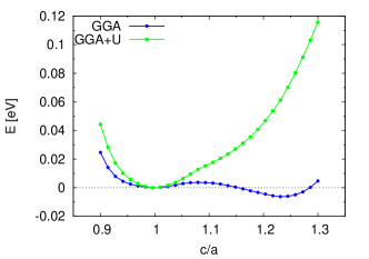
Figure 7: (Adapted from Ref. himmetoglu12_1 ; color online) The ground state energy as a function of $c/a$ for constant volume deformations in GGA and GGA+U.

where the energy profile as a function of the tetragonal distortion $c/a$ is shown ($c/a=1$ corresponding to the cubic austenite). As evident from the figure, the GGA functional achieves the minimum of the energy for an elongated tetragonal cell ($c/a\approx 1.1$) while experiments kokorin-modul ; martynov-modulated ; dai-eoa ; kaufmann-modulated report a martensitic phase consisting of a modulated tetragonal structure with $c/a\approx 0.97$. Since this specific value of $c/a$ is associated with the modulation of the structure, the cubic austenite phase should be obtained as the most stable one, when the modulation is neglected (as in the study presented here). Instead, non modulated tetragonal phases, with $c/a\geq 1$, are reported in experiments for off-stoichiometric compounds characterized, e.g., by excess Mn kokorin-modul ; sozinov02 .

From the density of states of the austenite phase (the one for the martensite would be similar), shown in Fig. 8, it is possible to observe that the states around the Fermi level (and thus responsible for the metallic character of the material) are mostly Ni $d$ states, while Mn $d$ states are largely responsible for the magnetization. In fact, the magnetic moments of Mn, Ni and Ga atoms are, respectively, $3.67\,\mu_{B},\,0.34\,\mu_{B}$ and $-0.13\,\mu_{B}$.

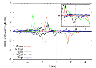
Figure 8: (Adapted from Ref. himmetoglu12_1 , color online) Density of states of the austenite phase calculated using GGA. The relevant symmetry groups of d-orbitals are explicitly indicated.

The discussion at the end of the previous section should clarify the reason why in Ref. himmetoglu12_1 the computational study of this material was performed with the FLL LDA+U corrective functional, selectively applied to the $d$ states of Mn. This strategy results in a more accurate description of the material, with larger magnetic moments on Mn atoms (see Table 1) and the austenite phase more stable than the non-modulated martensite one.

Table 1: Calculated lattice parameter and magnetizations of each atom in the cubic (austenite) phase of Ni₂MnGa.

	$a_{0}\,$ (Å)	$\mu_{\rm Mn}\,(\mu_{B})$	$\mu_{\rm Ni}\,(\mu_{B})$	$\mu_{\rm Ga}\,(\mu_{B})$	$\mu_{\rm tot}\,(\mu_{B}/{\rm cell})$
GGA	$5.83$	$3.67$	$0.34$	$-0.13$	$4.22$
GGA+U	$5.83$	$4.52$	$0.16$	$-0.13$	$4.80$

Fig. 7 compares the energy vs $c/a$ profiles obtained with GGA and GGA+U and highlights how the Hubbard correction eliminates the spurious minimum at $c/a>1$, predicting the cubic (austenite) phase more stable than any non-modulated tetragonal structure. In Ref. himmetoglu12_1 it is also shown that most of the variation in the total energy from the austenite to the martensite phase can be accounted for by a Heisenberg model of the total spin on Mn ions. In particular, computing (from constrained DFT calculations) the interatomic magnetic couplings $J$ in dependence of the tetragonal elongation and subtracting the corresponding Heisenberg term from the total energy, the minimum corresponding to the (non-modulated) martensite phase is eliminated. This result, due to the significant renormalization of the magnetic couplings induced by the Hubbard correction, can be rationalized by describing the localized $d$ electrons on Mn atoms as Anderson impurities interacting with a “bath” of more delocalized Ni $d$ and Ga $p$ electrons. In fact, the Anderson model results in RKKY effective interactions between Mn magnetic moments that have a clear dependence on the Hubbard $U$ (the parameter controlling the energy splitting between full and empty localized Hubbard bands). The Hubbard $U$ (as imposed by the Hubbard correction) suppresses magnetic interactions and reduces the energetic advantage associated with the deformation of the cubic austenite phase into a non modulated tetragonal martensite. As shown in Ref. himmetoglu12_1 , the FLL LDA+U on Mn $d$ states (with the effective $U$ calculated from linear-response theory as described in section III.3) is also able to capture the stabilization of a non-modulated tetragonal phase in compounds with excess Mn with respect to the stoichiometric composition.

This example shows that the use of the FLL LDA+U on the localized states of metals is not only possible, but actually very useful to capture, in certain cases, the effects of electronic localization, for example, on the magnetic and the structural properties of a material. In these instances, where a larger energy separation between Hubbard bands of localized states is needed to improve the description of the material, the LDA+U probably represents a more convenient choice than more sophisticated approaches (as DMFT) that are significantly more computationally demanding. On the other hand, the identification of the localized subset of states to be corrected by the LDA+U functional might not be as trivial as in the case described above, especially if the symmetry of the system is low. In these cases a scheme to automatically select localized states or able to treat localized and delocalized orbitals with equal accuracy would be highly desirable.

VI Extended functionals

VI.1 The LDA+U+V approach: when covalency is important

In this section we will briefly discuss one of the latest extensions to the LDA+U functional: the LDA+U+V campo10 . This modification is shaped on the “extended” Hubbard model and includes both on-site and inter-site electronic interactions. The extended formulation of the Hubbard Hamiltonian has been considered since the early days of this model hubbardIV ; hubbardV and can be expressed as follows:

$$H_{Hub}=t\sum_{\langle i,j\rangle,\sigma}(c^{\dagger}_{i,\sigma}c_{j,\sigma}+h.c.)+U\sum_{i}n_{i,\uparrow}n_{i,\downarrow}+V\sum_{\langle i,j\rangle}n_{i}n_{j}$$ (40)

where $V$ is the effective interaction between electrons on neighbor atomic sites.

The interest on the extended Hubbard model has been revamped in the last decades by the discovery of high T_c superconductors and the intense research activity focusing around them. Whether the inter-site coupling $V$ has a determinant role in inducing superconductivity is, however, still matter of debate andersonsci87 ; andersonprl87 ; imada91 ; hirsch88 ; thakur07 ; jursa96 ; szabo96 ; demello99 . Several studies have also demonstrated that the relative strength of $U$ and $V$ controls many properties of the ground state of correlated materials as, for example, the occurrence of possible phase separations mancini09 , the magnetic order morohoshi08 ; watanabe08 , the onset of charge-density and spin-density-wave regimes vandogen94 . In Refs. anisimov97 ; anisimov96 the inter-site coupling (between $d$ states) was recognized to be important to determine a charge-ordered ground state in mixed-valence systems, while in Ref. verdozzi95 the extended Hubbard Hamiltonian was used to refine the Auger core-valence-valence line shapes of solids. More recently, the extended Hubbard model has been used to study the conduction and the structural properties of polymers and carbon nano-structures and it was shown that the interplay between $U$ and $V$ controls the dimerization of graphene nanoribbons zhu06 .

Our motivation to include inter-site interactions in the formulation of the corrective Hubbard Hamiltonian was the attempt to define a more flexible and general computational scheme able to precisely account for (rather than just suppress) the possible hybridization of atomic states on different atoms. In order to understand the implementation of the LDA+U+V campo10 it is useful to start from a (mean-field-factorized) second-quantization expression of the electronic interaction energy with a full set of site- and orbital- dependent interactions:

$$E_{int} = \frac{1}{2}\sum_{I,J,K,L}\sum_{i,j,k,l}\sum_{\sigma}\>\langle\phi^{I}_{i}\phi^{J}_{j}|V_{ee}|\phi^{K}_{k}\phi^{L}_{l}\rangle\>\times$$ (41)

$$\left(n^{KI\sigma}_{ki}n^{LJ\sigma^{\prime}}_{lj}-\delta_{\sigma\sigma^{\prime}}n^{KJ\sigma}_{kj}n^{LI\sigma^{\prime}}_{li}\right)$$

where the numbers $n^{KI\sigma}_{ki}$ represent the average values of products of creation and annihilation fermion operators ($\langle{c^{I\sigma}_{i}}^{\dagger}c^{K\sigma}_{k}\rangle$), to be associated to generalized occupations, defined as:

$$n^{IJ\sigma}_{mm^{\prime}}=\sum_{k,v}f_{kv}^{\sigma}\langle\psi_{kv}^{\sigma}|\phi_{m^{\prime}}^{J}\rangle\langle\phi_{m}^{I}|\psi_{kv}^{\sigma}\rangle.$$ (42)

In Eq. (42) the indices $m$ and $m^{\prime}$ run over the angular momentum manifolds that are subjected to the Hubbard correction on atoms $I$ and $J$ respectively. It is important to notice that the occupation matrix defined in Eq. (42) contains information about all the atoms in the same unit cell and the on-site occupations defined in Eq. (3) correspond to its diagonal blocks (${\rm\bf n}^{I\sigma}={\rm\bf n}^{II\sigma}$). Generalizing the approach described for the on-site case, the $E_{Hub}$ term of the DFT+U+V can be obtained from Eq. (41) retaining only those terms that contain the interaction between orbitals belonging to couples of neighbor atomic sites: $\langle\phi^{I}_{i}\phi^{J}_{j}|V_{ee}|\phi^{K}_{k}\phi^{L}_{l}\rangle\to\delta_{IK}\delta_{JL}\delta_{ik}\delta_{jl}V^{IJ}+\delta_{IL}\delta_{JK}\delta_{il}\delta_{jk}K^{IJ}$. Similarly to the on-site case, the effective inter-site interactions are assumed to be all equal to their atomic averages over the states of the two atoms: $\langle\phi^{I}_{i}\phi^{J}_{j}|V_{ee}|\phi^{K}_{k}\phi^{L}_{l}\rangle\to\delta_{IK}\delta_{JL}\delta_{ik}\delta_{jl}V^{IJ}=\frac{\delta_{IK}\delta_{JL}\delta_{ik}\delta_{jl}}{(2l_{I}+1)(2l_{J}+1)}\sum_{i^{\prime},j^{\prime}}\langle\phi^{I}_{i^{\prime}}\phi^{J}_{j^{\prime}}|V_{ee}|\phi^{I}_{i^{\prime}}\phi^{J}_{j^{\prime}}\rangle$. Within this hypothesis, and assuming that the inter-site exchange couplings $K^{IJ}$ can be neglected, it is easy to derive the following expression ($U^{I}=V^{II}$):

$$E_{Hub} = \sum_{I}\frac{U^{I}}{2}\left[\>(n^{I})^{2}-\sum_{\sigma}Tr\left[({\rm\bf n}^{II\sigma})^{2}\right]\>\right]$$ (43)

$$+ \sum_{IJ}^{\hskip 14.22636pt\star}\frac{V^{IJ}}{2}\left[n^{I}n^{J}-\sum_{\sigma}Tr({\rm\bf n}^{IJ\sigma}{\rm\bf n}^{JI\sigma})\right]$$

where the star in the second summation operator reminds that for each atom $I$, index $J$ covers all its neighbors up to a given shell. Generalizing the FLL expression of the on-site double-counting term to include inter-site interactions, we arrive at the following expression:

$$E_{dc}=\sum_{I}\frac{U^{I}}{2}n^{I}(n^{I}-1)+\sum_{I,J}^{\hskip 14.22636pt\star}\frac{V^{IJ}}{2}n^{I}n^{J}.$$ (44)

Subtracting Eq. (44) from Eq. (43) it is easy to obtain:

$$E_{UV} = E_{Hub}-E_{dc}=\sum_{I,\sigma}\frac{U^{I}}{2}Tr\left[{\rm\bf n}^{II\sigma}\left({\bf 1}-{\rm\bf n}^{II\sigma}\right)\right]$$ (45)

$$- \sum_{I,J,\sigma}^{\hskip 14.22636pt*}\frac{V^{IJ}}{2}Tr\left[{\rm\bf n}^{IJ\sigma}{\rm\bf n}^{JI\sigma}\right].$$

To better understand the role of the inter-site part of the energy functional it is convenient to derive the correction it contributes to the (generalized) KS potential:

$$V_{UV} = \sum_{I,m,m^{\prime}}\frac{U^{I}}{2}\left(\delta_{mm^{\prime}}-2n^{II\sigma}_{mm^{\prime}}\right)|\phi^{I}_{m}\rangle\langle\phi^{I}_{m^{\prime}}|$$ (46)

$$- \sum_{I,J,m,m^{\prime}}^{\hskip 14.22636pt*}V^{IJ}n^{JI\sigma}_{mm^{\prime}}|\phi^{I}_{m}\rangle\langle\phi^{J}_{m^{\prime}}|.$$

From Eq. (46) it is evident that while the on-site term of the potential is attractive for occupied states that are, at most, linear combinations of atomic orbitals of the same atom (resulting in on-site blocks of the occupation matrix, ${\rm\bf n}^{II\sigma}$, numerically dominant on others), the inter-site interaction stabilizes states that are linear combinations of atomic orbitals belonging to distinct (neighbor) atoms (e.g., molecular orbitals), that lead to large inter-site blocks ${\rm\bf n}^{JI\sigma}$ of the occupation matrix. Thus, the two interactions give rise to competing tendencies, and the character of the resulting ground state depends on the balance between them. Fortunately, the linear-response calculation of the effective interactions, discussed in section III and in Ref. cococcioni05 , offers the possibility to compute both parameters simultaneously (and with no additional cost with respect the on-site case). In fact, the inter-site couplings $V^{IJ}$ correspond to the off-diagonal terms of the interaction matrix defined in Eq. (27).

It is important to stress again that the trace operator in the on-site functional guarantees the invariance of the energy only with respect to rotations of atomic orbitals on the same atomic site. In fact, the on-site corrective functional (Eq. (13)) is not invariant for unitary transformations of the atomic orbital basis set that mix states from different atoms. With the “+U+V” corrective functional the invariance with respect to general rotations within the atomic basis set would be exactly recovered in the limit situation with the same $U$ on all the atoms and equal to all the $V$ between them ($U=V$). In fact, in this case, the sum of on-site and inter-site interactions in Eq. 45 would be proportional to the trace of the square of the generalized occupation matrix in Eq. 42. In the most general case, the differentiation between the interaction parameters would require full orbital dependence for the corrective functional to be invariant. Atomic center and angular momentum dependence of the corrective functional are implicitly included in Wannier-function-based implementations of the LDA+U oregan10 ; oregan12 ; fabris05 ; fabris05_1 ; mazurenko07 ; lechermann06 ; miyake08 . In fact, even starting from an on-site only formulation, re-expressing Wannier functions on the basis of atomic wave functions produces a variety of multi-center/multi-orbital interaction terms. The two approaches would thus lead to equivalent results if all the relevant multiple-center interactions parameters are included in the corrective functionals and are computed consistently with the choice of the orbital basis. While the use of Wannier-functions allows to minimize the number of relevant electronic interactions to be computed (especially if maximally-localized orbitals are used marzari97 ), the atomic orbital representation provides a more intuitive and transparent scheme to select relevant interactions terms (e.g., based on inter-atomic distances), and is more convenient to compute derivatives of the energy as, for example, forces and stresses.

In the implementation of Eq. (45) we have added the possibility for the corrective functional to act on two $l$ manifolds per atom as, for example, the $3s$ and $3p$ orbitals of Si, or the $4s$ and $3d$ orbitals of Ni. The motivation for this extension consists in the fact that different manifolds of atomic states may require to be treated on the same theoretical ground in cases where hybridization is relevant (as, e.g., for bulk Si whose bonding structure is based on the $sp^{3}$ mixing of $s$ and $p$ orbitals).

The new LDA+U+V functional was first employed to study the electronic and structural properties of NiO, Si and GaAs campo10 , prototypical representatives of Mott or charge-transfer (NiO) and band insulators (Si and GaAs). The choice of these systems was made to test the ability of the new functional to bridge the description of the two kinds of insulators. In fact, as discussed in previous sections (see Eq. (15)), the fundamental gap of a system is the sum of the KS gap and the discontinuity in the xc potential (usually missing in most approximate local or semi-local xc functionals) grosslibro . Since the “+U” correction was designed to reintroduce the discontinuity into the xc potential, LDA+U should be equally effective in improving the prediction of the fundamental gap (from the KS spectrum) for both types of materials, and it can be expected to improve the prediction of other properties too.

As other transition-metal oxides, NiO has a cubic rocksalt structure with a rhombohedral symmetry brought about by its AF II ground state. Because of the balance between crystal field and exchange splittings of the $d$ states of Ni, nominally occupied by 8 electrons, the material has a finite KS gap with oxygen $p$ states occupying the top of the valence band. This gap, however, severely underestimates the one obtained from photoemission experiments (of about 4.3 eV sawatzky84 ). LDA+U has been used quite succesfully on this material (the spread of results in literature is mostly due to the different values of $U$ used) providing a band gap between 3.0 and 3.5 eV, and quite accurate estimates for both magnetic moments and equilibrium lattice parameter dudarevnio00 ; bengone00 ; kressenio04 . DFT+U has also been employed to compute the $k$-edge XAS spectrum of NiO using a parameter-free computational approach maurinio09 that has produced results consistent with experimental data. The use of GW from the LDA+U ground state has provided a better estimate of the energy gap compared to LDA+U, even though other details of the density of states were almost unchanged  kobayashi08 .

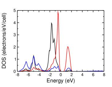
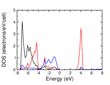
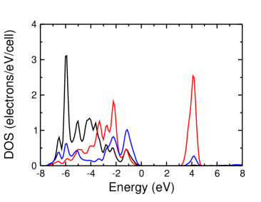
Figure 9: (Reprint of Fig. 2 of Ref. campo10 ; color online) The density of states of NiO obtained with different approximations: GGA (top); GGA+U (center); GGA+U+V (bottom). spin $d$ states of Ni, the blue line the $p$ states of O. The energies were shifted for the top of the valence band to correspond to the zero of the energy in all cases. The black line represents majority spin $d$ states, the red line minority $d$ states, the blue line oxygen $p$ states.

Besides the on-site $U_{Ni}$, the LDA+U+V calculations also included the interactions between nearest neighbor Ni and O ($V_{Ni-O}$) and between second nearest neighbor Ni atoms ($V_{Ni-Ni}$). The corrective functional included interactions between the $d$ states of Ni, between Ni $d$ and O $p$ states and between $d$ and $s$ states of the Ni atoms. Other interactions were found to have a negligible effect on the results and were neglected. The numerical values of the interaction parameters, all determined through the linear-response approach discussed above, can be found in Ref. campo10 . Fig. 9 compares the density of states (DOS) of NiO as obtained from GGA, GGA+U and GGA+U+V calculations. It is easy to observe that the GGA+U+V obtains a band gap of the same width as GGA+U, also maintaining the charge-transfer character of the material with O $p$ states at the top of the valence band, as observed in photoemission experiments. On the contrary, the GGA band gap is too small compared with experiments and also has Ni $d$ states at the top of the valence band. As expected, the inter-site interactions between Ni and O electrons also results in a more pronounced overlap in energy between $d$ and $p$ states.

Table 2: The equilibrium lattice parameter, ($a$, in Bohr atomic radii), the bulk modulus ($B$, in GPa), and the band gap ($E_{g}$, in eV) of NiO obtained with different computational approaches: GGA, “traditional” GGA+U (with U only on the $d$ states of Ni) and GGA+U+V with the interaction parameters computed “self-consistently” from the GGA+U+V ground state (see text). Comparison is made with experimental results on all the computed quantities.

	$a$	$B$	$E_{g}$
GGA	7.93	188	0.6
GGA+U	8.069	181	3.2
GGA+U+V	7.99	197	3.2
Exp	7.89	166-208	3.1-4.3

In table 2 a comparison is made between experiments and calculations on the equilibrium lattice parameter, bulk modulus and energy gap. It can be observed that while GGA provides the best estimate of the experimental lattice parameter, GGA+U+V improves on the result of GGA+U for the lattice parameter and the bulk modulus is also corrected towards the experimental value. Therefore, accounting for inter-site interactions not only is not detrimental for the quality of the LDA+U description of the ground state of correlated materials but also has the potential to improve problematic aspects (e.g., structural properties) counter-balancing the effects of eccessive electronic localization.

The application to Si and GaAs is, in some sense, the “proof of fire” for the LDA+U+V approach, as the insulating character of these materials is due to the hybridization of $s$ and $p$ orbitals from neighbor atoms which leads to a finite splitting between the energy of fully occupied (bonding) and empty (anti-bonding) states. The eccessive stabilization of atomic orbitals induced by the on-site $U$ suppresses the overlap with neighbor atoms and tends to reduce the gap between valence and conduction states campo10 . While providing a quite good description of the ground state properties of these materials, the Kohn-Sham gap obtained from LDA and GGA functionals is significantly smaller than the experimental band gap. Although this is an expected result, corrective methods able to enforce the discontinuity to the xc potential and to improve the size of the fundamental gap, are also beneficial for predicting other properties, and the same can be expected from using Hubbard corrections. A more accurate estimate of the band gap of these materials has been obtained using SIC and hybrid functionals stadele99 ; nguyen09 ; heyd05 or with the GW approach based on an LDA rohlfing93 ; aulbur99 or a EXX aulbur00 ground state.

As mentioned above, for the LDA+U+V method to work on these systems and to capture the $sp^{3}$ hybridization their bonding structure is based on, the Hubbard correction has to be applied to both $s$ and $p$ states and to include a full spectrum of on-site ($U_{pp}$, $U_{ss}$, $U_{sp}$) and inter-site interactions ($V_{pp}$, $V_{ss}$, $V_{sp}$). The linear-response approach to calculate the effective Hubbard $U$, described in section III, allowed to reliably compute all these intereaction parameters and to capture their dependence on the volume of the crystal. In Table 3, the equilibrium lattice parameter, the bulk modulus and the energy band gap obtained from GGA, GGA+U and GGA+U+V calculations on Si and GaAs can be directly compared with the results of experimental measurements (we refer to the data collected in the web-database, Ref. semicondbase ).

Table 3: Comparative results for lattice parameter ($a$, in ${\rm\AA}$), bulk modulus (B, in GPa) and energy gap ($E_{g}$, in eV).

	Si	GaAs
	$a$      B      $E_{g}$	$a$      B      $E_{g}$
GGA	5.479, 83.0, 0.64	5.774, 58.4, 0.19
GGA+U	5.363, 93.9, 0.39	5.736, 52.6, 0.00
GGA+U+V	5.370, 102.5, 1.36	5.654, 67.7, 0.90
Exp.	5.431, 98.0, 1.12	5.653, 75.3, 1.42

As it can be observed from this table, the (on-site only) GGA+U predicts the equilibrium lattice parameter in better agreement with the experimental value than GGA for GaAs while it overcorrects GGA for Si; however, the bulk modulus is improved by GGA+U with respect to the GGA value only in the case of Si. Due to the suppression of the interatomic hybridization, in both cases, the energy band gap is lowered compared to GGA, further worsening the agreement with experiments. The use of the inter-site correction results in a systematic improvement for the evaluation of all these quantities. In fact, encouraging the occupations of hybrid states, the inter-site interactions not only enlarge the splittings between full and empty levels (which increases the size of the band gap), but also make bonds shorter (so that hybridization is enhanced) and stronger, thus tuning both the equilibrium lattice parameter and the bulk modulus of these materials to values closer to the experimental data. Calculations on GaAs explicitly included Ga $3d$ states in the valence manifold as suggested by Ref. schultz08 .

Figure 10: (From Fig. 4 of Ref. campo10 ) The band structure of Si (top) and GaAs (bottom). Continuous lines represent GGA+U+V results and dashed lines represent standard GGA results. All energies were shifted so that the top of valence bands are at zero energy.

Fig. 10 shows a comparison between the band structures of Si and GaAs obtained with GGA and GGA+U+V. It is evident from the figure that the increase in the band gap obtained with the “+U+V” correction is the result of an almost uniform shift of electronic energies (downward for valence, upwards for conduction states) that maintains the overall dispersion pattern.

These results confirm that the extended Hubbard correction is able to significantly improve the description of band insulators and semiconductors with respect to GGA, providing a more accurate estimate of structural and electronic properties. In view of the fact that these systems are normally treated with hybrid functionals or SIC approaches, the good results obtained with LDA+U+V are the demonstration that this approach has similar capabilities. The inaccuracy of the LDA+U (with on-site interactions only) is not inherent to the reference model but rather to the approximations used in its final expression. These results also clarify that, within the single particle KS representation of the $N$-electron problem, band and Mott insulators can be treated with similar corrective approaches.

The fact that LDA+U+V can be equally accurate in the description of band and Mott insulators opens to the possibility to use it in a broad range of intermediate situations where (Mott) electronic localization coexists with or competes against the hybridization of atomic states from neighbor atoms, (as, e.g., in magnetic impurities in semiconductors or metals, high T_c superconductors, etc), or in the description of processes (such as, e.g., electronic charge transfers excitation himmetoglu12_2 ) involving a significant variation in the degree of electronic localization.

In a recent work kulik11_1 LDA+U+V was used to study transition-metal dioxide molecules (e.g., MnO₂). The inclusion of the inter-site interaction was found to be crucial to predict the electronic configuration, the equilibrium structure and its deformations in agreement with experiments. The extended corrective functional has also been used as the starting point of DFT+DMFT calculations and it has been demonstrated that the inclusion of the inter-site interaction at a static mean-field level (with the DMFT calculation performed on atomic impurities) produced results of the same quality of more computationally intensive cluster-DMFT calculations anisimov12 .

More recently, LDA+U+V has been used to calculate the lowest excited state energies of phosphorescent Ir dyes himmetoglu12_2 using the $\Delta$-SCF method ziegler77 . These molecular complexes are widely used as sensitizers in organic electronic devices baldo98 ; holmes09 . In fact, the strong spin-orbit coupling that characterizes their metallic centers, is able to change the spin state of the photo-excited electron-hole pair from singlet to triplet, thus extending its life-time (the recombination process is significantly inhibited by selection rules) and improving the efficiency of the device.

Approximate DFT functionals yield a poor description of the electronic properties of these systems due to the localization of electrons on Ir $d$ orbitals. The excited states of these molecules are of metal-to-ligand charge transfer (MLCT) type, as illustrated in Fig. 11 for one of the studied molecules, Ir(ppy)₃.

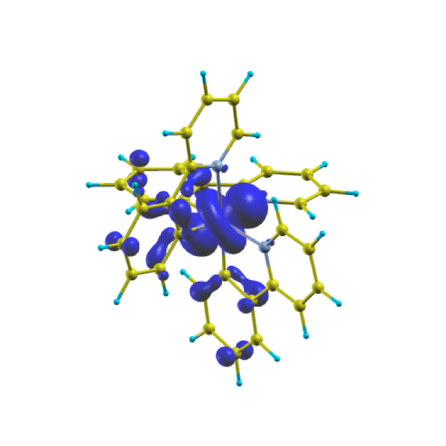
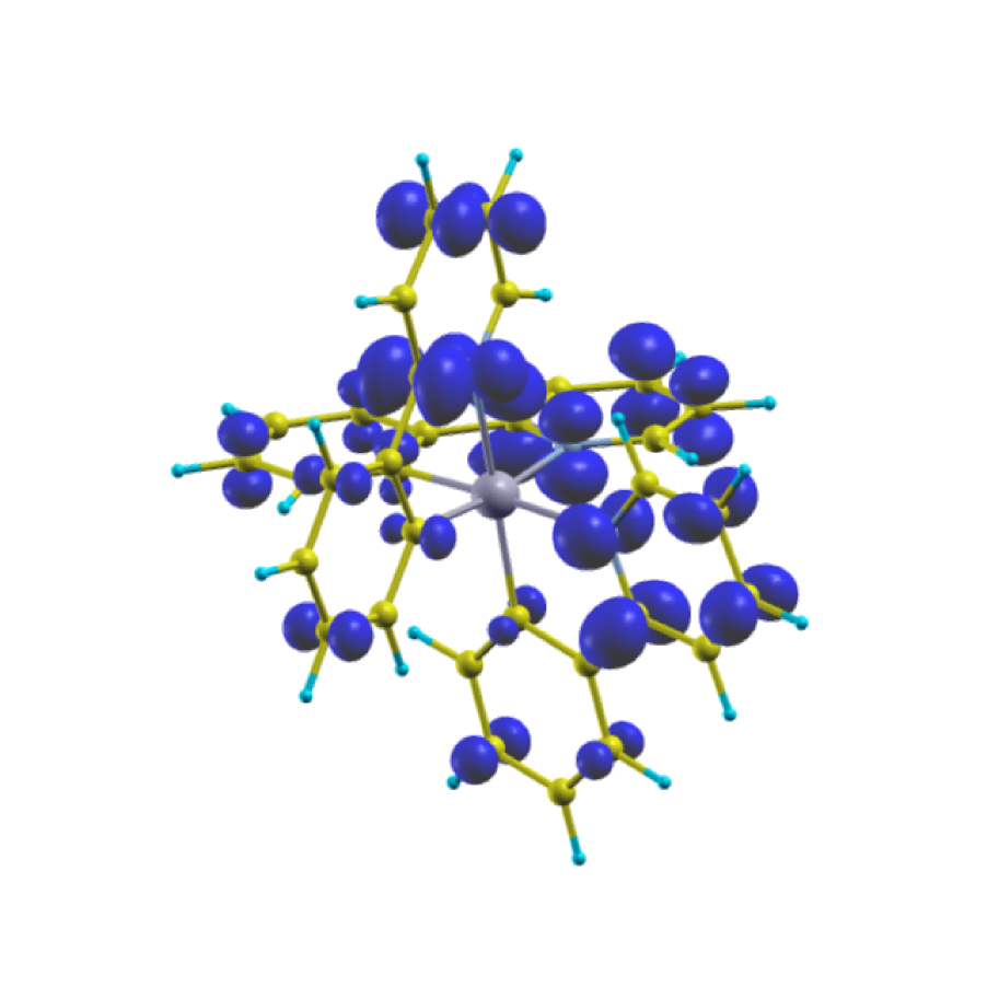
Figure 11: (Adapted from Ref. himmetoglu12_2 ; color online) Ir(ppy)₃ HOMO(left) and LUMO(right) calculated using the ground-state electronic density.

Consequently, an accurate calculation of excited state energies requires that the functional used is able to capture the localization of electrons on the $d$ orbitals of Ir as well as their possible hybridization with the organic ligands. In Ref himmetoglu12_2 it has been shown that a straight use of the Hubbard $U$ correction on Ir $d$ orbitals overlocalize electrons on the metal center, suppresses their hybridization with organic ligands, and results in a poor estimate of excited state energies. Instead, the Hubbard $V$ between the $d$ orbitals of Ir and those of neighbor atoms in the organic ligands corrects for the over-localization and gives results in good agreement with experiments himmetoglu12_2 . TDDFT can also be used to study the excitation energies of this system; however, the MLCT character of these excitation imposes the use of hybrid functionals that allow to capture the non-locality of the electronic interactions.

Table 4: $\Delta$-SCF and TDDFT calculations of the lowest triplet and singlet states for three phosphorescent dyes: Ir(ppy)₃, FIrpic, and PQIr (data from himmetoglu12_2 ). All values are in $eV$ and measured from the ground state energy. The +U+V result is the one obtained after a preliminary structural optimization of the molecule with this approach. TDDFT results were obtained with the Gaussian code g09 , using M06 m06 hybrid functionals.

Ir(ppy)3	GGA	U	TDDFT	U+V	Exp
T	2.32	2.27	2.55	2.44	2.4
S [NSP]	2.50	2.90	2.79	2.73	2.6-2.7
$\Delta\,E_{\rm TS}$ [NSP]	0.18	0.62	0.24	0.29	0.2-0.3
FIrpic	GGA	U	TDDFT	U+V	Exp
T	2.46	2.79	2.66	2.52	2.6
S [NSP]	2.65	3.00	3.0	2.81	3.3-2.9
$\Delta\,E_{\rm TS}$ [NSP]	0.18	0.20	0.34	0.29	0.3-0.7
PQIr	GGA	U	TDDFT	U+V	Exp
T	1.81	2.11	2.01	1.90	2.1
S [NSP]	2.01	2.34	2.37	2.18	2.3
$\Delta\,E_{\rm TS}$ [NSP]	0.19	0.23	0.36	0.28	0.2

Table 4 summarizes the excitation energies computed with LDA+U+V $\Delta$-SCF and TDDFT techniques for three Ir phosphorescent complexes (Ir(ppy)₃, FIrpic, and PQIr) considered in Ref. himmetoglu12_2 and compares them with GGA and GGA+U $\Delta$-SCF calculations and available experimental data. These results show that LDA+U+V represent a viable alternative to more computationally intensive hybrid functionals to compute (either by $\Delta$-SCF or TDDFT) excitation energies that involve electron transfer processes. Ref. himmetoglu12_2 also rationalized the dependence of HOMO and LUMO energies in these molecules on the values of the Hubbard $U$ (on Ir $d$ states) and $V$ (between Ir and its C and N nearest neighbors) showing a predictable behavior of these excitation energies. These observations may provide valuable informations to tune the performance of these molecules through the screening of substitutional impurities in their ligand complexes.

VI.2 DFT+U+J: Magnetism and localization

While invariance is unanimously recognized as a necessary feature of the corrective functional, whether to use the full rotational invariant correction, Eqs. (II.2) and (II.2), or its simpler version, Eq. (13), has often appeared as a matter of taste and has been dictated by the availability of either implementation in current codes. In fact, the two corrective schemes give very similar results for a large number of systems in which electronic localization is not critically dependent on Hund’s rule magnetism. However, as mentioned in section II.3, in some materials that have recently attracted considerable interest, this equivalence does not hold and the explicit inclusion of the exchange interaction ($J$) in the corrective functional appears to be necessary. Examples of systems in this group include recently discovered Fe-pnictides superconductors nakamura09 , heavy-fermion bultmark09 ; pickett06 , non-collinear spin materials spaldin10 , or multiband metals, for which the Hund’s rule coupling, promotes, depending on the filling of localized states, metallic or insulating behaviors demedici11 ; georges11 . In our recent work on CuO himmetoglu11 the necessity to explicitly include the Hund’s coupling $J$ in the corrective functional was determined by a competition (likely to exist in other Cu compounds as well, such as high T_c superconductors), between the tendency to complete the external 3$d$ shell and the onset of a magnetic ground state (dictated by Hund’s rule) with 9 electrons on the $d$ manifold. The precise account of exchange interactions between localized $d$ electrons beyond the simple approach of Eq. (13) (with $U_{eff}=U-J$) turned out to be crucial to predict the electronic and structural properties of this material. In this work we used a simpler $J$-dependent corrective functional than the full rotationally invariant one to achieve this goal. The expression of the functional can be obtained from the full second-quantization formulation of the electronic interaction potential, given in Eq. (41), by keeping only on-site terms that describe the interaction between up to two orbitals. Approximating on-site effective interactions with the (orbital-independent) atomic averages of Coulomb and exchange terms, $U^{I}=\frac{1}{(2l+1)^{2}}\,\sum_{i,j}\langle\phi_{i}^{I}\phi_{j}^{I}|V_{ee}|\phi_{i}^{I}\phi_{j}^{I}\rangle$ and $J^{I}=\frac{1}{(2l+1)^{2}}\,\sum_{i,j}\langle\phi_{i}^{I}\phi_{j}^{I}|V_{ee}|\phi_{j}^{I}\phi_{i}^{I}\rangle$, it is easy to derive the following expression:

$$E_{U+J}=E_{\rm Hub}-E_{\rm dc} = \sum_{I,\,\sigma}\,\frac{U^{I}-J^{I}}{2}\,{\rm Tr}[{\bf n}^{I\,\sigma}\,({\bf 1}-{\bf n}^{I\,\sigma})]$$ (47)

$$+ \sum_{I,\,\sigma}\,\frac{J^{I}}{2}\,{\rm Tr}[{\bf n}^{I\,\sigma}\,{\bf n}^{I\,-\sigma}].$$

Comparing Eqs. (13) and (47), one can see that the on-site Coulomb repulsion parameter ($U^{I}$) is effectively reduced by $J^{I}$ for interactions between electrons of parallel spin and a positive $J$ term further discourages anti-aligned spins on the same site, stabilizing magnetic ground states. The second term on the right-hand side of equation (47) can be explicated as $\sum_{I,\sigma}\,(J^{I}/2)\,\sum_{m,m^{\prime}}n^{I\,\sigma}_{m\,m^{\prime}}\,n^{I\,-\sigma}_{m^{\prime}\,m}$ which shows how it corresponds to an “orbital exchange” between electrons of opposite spins (e.g., up spin electron going from $m^{\prime}$ to $m$ and down spin electron from $m$ to $m^{\prime}$). It is important to notice that this term is genuinely beyond Hartree-Fock. In fact, a single Slater determinant containing the four states $m\uparrow$ , $m\downarrow$, $m^{\prime}\uparrow$ , $m^{\prime}\downarrow$ would produce no interaction term like the one above. Thus, the expression of the $J$ term given in equation (47), based on the product of ${\bf n}^{I\,\sigma}$ and ${\bf n}^{I\,-\sigma}$ is an approximation of a functional that would require the calculation of the 2-body density matrix to be properly included. However, the $J$ term in Eq. (47) can be regarded as the one needed to eliminate a term in the spurious curvature of the energy deriving from the interaction between antiparallel spins. Therefore, its formulation and use in corrective functionals are legitimate. Similar terms in the corrective functional have already been proposed in literature demedici11 ; georges11 ; quan11 ; yoshitake11 ; pavarinibook11 , although within slightly different functionals.

Eq. (47) represents a significant simplification with respect to Eqs. (II.2) and (II.2) and proved crucial to predict the insulating character of the cubic phase of CuO himmetoglu11 .

Unlike other transition metal monoxides (all rhombohedral), CuO has a monoclinic unit cell. In addition, while exhibiting a similar antiferromagnetic ground states (with ferromagnetic planes of Cu atoms alternating with opposite spins - the so-called AFII order), its Neél temperature is significantly lower than predicted from the trend of other materials in this class, suggesting a weaker magnetic interaction between Cu ions. Although it is not the equilibrium structure of this system, the perfectly cubic crystal has been considered as a limiting case of the tetragonal phase grown on selected substrates siemons2009tetragonal or as a proxy system to study the electronic properties of cuprate superconductors grant2008electronic . While the analogy with other transition metal monoxides would suggest an insulating behavior, the cubic phase was invariably predicted to be metallic by approximate DFT, LDA+U and hybrid functional calculations grant2008electronic ; peralta2009jahn ; chen2009hybrid . This outcome is due to a “double” (orbital and spin) degeneracy between the highest energy $e_{g}$ states of each Cu atom where a hole should appear (Cu are nominally in a 2+ oxidation state). As explained in section II.4, these degeneracies need to be lifted if a gap is to appear in the Kohn-Sham spectrum of the material. It is important to notice that the two degeneracies are mutually reinforcing: if spin states have the same energy the material is not magnetic and the symmetry of the crystal is perfectly cubic with an exact degeneracy between $e_{g}$ states. The use of a triclinic super cell of the cubic structure, depicted in Fig. 12,

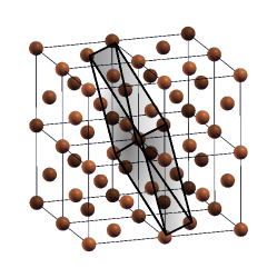
Figure 12: The triclinic supercell used for calculations. Only the Cu atoms are shown for clarity.

and an AFII magnetic order are sufficient to lift both these symmetries. However, no insulating state is obtained if $J$ is set to 0. In fact, the presence of the $p$ states of oxygen at the top of the valence band together with Cu $d$ states makes the partial occupation of both manifolds more energetically favorable than the localization of holes on the $d$ states of Cu atoms (as necessary to obtain a finite magnetization). In particular, a magnetic ground state with an inbalance of population between Cu $d$ states of opposite spin and a (approximately) complete O $p$ manifold has a slightly higher energy than a non magnetic ground state with a larger number of electrons on Cu $d$ states (thus closer to complete its $d$ shell) equally distributed between the two spin, and a hole spread between $d$ and $p$ levels that results in a metallic ground state. A finite Hund’s coupling $J$ favors the magnetic ground state, also resulting in the complete localization of the hole on the Cu $d$ states and in the formation of a band gap. The total energy of the cubic phase (insulating ground state) as a function of the tetragonal distortion, shown in Fig. 13,

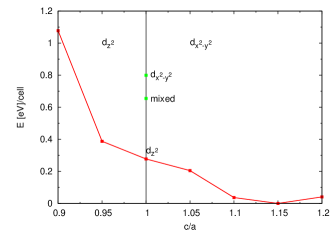
Figure 13: (Adapted from Ref. himmetoglu11 ; color online) Total state energy profile of CuO in the LDA+U+J insulating ground state as a function of $c/a$.

presents a monotonic profile (although the material shows a different orbital ordering with a hole occupying the $z^{2}$ state of Cu for $c/a<1$ and the $x^{2}-y^{2}$ for $c/a>1$).

The energy profile shown in Fig. 13 was obtained recomputing the interaction parameters for every value of $c/a$. $U$, in particular, was calculated self-consistently, using the linear-response approach illustrated in section III.3 on the LDA+U+J ground state of the system (results are shown in Fig. 8 of Ref. himmetoglu11 ). The $J$, instead, was computed (through a generalization of the linear-response technique based on the perturbative potential of Eq. (29)), only from the non magnetic GGA ground state of the cubic phase and the same value was used for all the considered $c/a$ and lattice parameters. In fact, as explained in section III.3, the linear response procedure applied to $m^{I}$ is less reliable and technically more difficult to apply when atoms assume a finite magnetization. Furthermore, the smooth variation of $U_{sc}$ (about 1 eV from $c/a=0.9$ to $c/a=1.2$), shown in Fig. 8 of Ref. himmetoglu11 suggests that the variation of $J$ with the lattice parameter and $c/a$ can be safely neglected.

The monotonic decrease of the energy of the system with the tetragonal distortion of its unit cell, is in contrast with previous studies peralta2009jahn ; chen2009hybrid that obtained a double-well energy profile with two minima corresponding to tetrahedral phases with $c/a<1$ and $c/a>1$, respectively, but in agreement with experiments that reported a stable structure only for $c/a>1$. The LDA+U+J functional was also able to predict the existence of several orbital-ordered states (with the hole hosted on different $d$ orbitals on different Cu atoms) whose energy is not much higher than the ground state one, as indicated in Fig. 13. We argue that these states can play an important role at finite temperature in this and similar Cu-O-based materials.

The study of CuO illustrates the effectiveness of the LDA+U+J in capturing the ground state of systems where (intra-atomic, Hund’s type) magnetic interactions play an important role in determining the localization of electrons on strongly correlated orbitals. The simplicity of the formulation of the “+U+J” corrective functional of Eq. (47) greatly facilitates its use and the implementation of other algorithms (such as, for example, the calculation of forces, stresses cococcioni10 and phonons floris11 ), discussed in section VII, that will be crucial to study, for example, the lattice vibration of systems characterized by a strong Hund’s coupling on strongly localized electrons.

More complex aspects of magnetism in strongly correlated materials require the LDA+U to be extended to a non-collinear spin formalism, as done, for example, in Ref. spaldin10 . This implementation is, in fact, crucial to study correlated systems characterized by canted magnetic moments, strong spin-orbit interactions and magnetic anisotropy (quite common in rare earth compounds) pickett06 , spin-wave excitations (magnons) essenberger11 . Due to the quantity of both formal and physical aspects that would be necessary to discuss for its thorough tractation, this extension of the LDA+U method will not be presented in this work, and the interested reader is encouraged to refer to the above mentioned literature for details.

VII Energy derivatives

One of the most important advantages brought about by the simple formulation of the LDA+U corrective functional is the possibility to easily and efficiently compute total energy derivatives, as forces, stresses, dynamical matrices, etc. These are crucial quantities to identify and characterize the equilibrium structure of materials under different physical conditions, to study the vibrational properties, to perform molecular dynamics calculations and to account for finite ionic temperature effects (typically dominant in insulators). In this section we will review the formalism to calculate forces, stresses, and second derivatives from a LDA+U ground state (Refs. cococcioni10 ; floris11 for details). For most of its part we will assume that the variation of $U$ with the ionic positions and/or the lattice parameters can be neglected; the importance of varying $U$ will be discussed in Sec. VII.4. In the derivation of the Hubbard contribution to total energy derivatives, we will also assume a corrective functional based on atomic orbitals as localized basis sets. This derivation can be easily generalized to other basis sets, provided that the derivative of their localized orbitals can be computed analytically.

VII.1 The Hubbard forces

The Hubbard forces are defined as the negative derivatives of the Hubbard energy with respect to the atomic displacements. Taking the derivative of $E_{U}$ in Eq. (13) it is easy to arrive at the expression:

$$F^{U}_{\alpha,i} = -\frac{\partial E_{U}}{\partial\tau_{\alpha i}}=-\sum_{I,m,m^{\prime},\sigma}\frac{\partial E_{U}}{\partial n^{I\sigma}_{m,m^{\prime}}}\frac{\partial n^{I\sigma}_{m,m^{\prime}}}{\partial\tau_{\alpha i}}$$ (48)

$$= -\frac{U}{2}\sum_{I,m,m^{\prime},\sigma}(\delta_{mm^{\prime}}-2n^{I\sigma}_{m^{\prime}m})\frac{\partial n^{I\sigma}_{m,m^{\prime}}}{\partial\tau_{\alpha i}}$$

where $\delta\tau_{\alpha i}$ is the atomic displacement and $n^{I\sigma}_{m,m^{\prime}}$ are the occupation matrices, defined in Eq. (3). Since the Hellmann-Feynman theorem applies for energy first order derivatives, no response of the electronic wave function has to be taken into account and the symbol $\partial$ indicates only the explicit (“bare”) derivative with respect to atomic positions. Based on the definition in Eq. (3) it is easy to work out the formula for the derivative of the atomic occupations:

$$\frac{\partial n^{I\sigma}_{m,m^{\prime}}}{\partial\tau_{\alpha i}} = \sum_{k,v}f_{kv}[\frac{\partial}{\partial\tau_{\alpha i}}(\langle\psi^{\sigma}_{kv}|\phi^{I}_{m^{\prime}k}\rangle)\langle\phi^{I}_{mk}|\psi^{\sigma}_{kv}\rangle$$ (49)

$$+ \langle\psi^{\sigma}_{kv}|\phi^{I}_{m^{\prime}k}\rangle\frac{\partial}{\partial\tau_{\alpha i}}\left(\langle\phi^{I}_{mk}|\psi^{\sigma}_{kv}\rangle\right)]$$

where $k$ and $v$ are k-point and band indexes, respectively. The problem is then reduced to calculate the quantities

$$\frac{\partial}{\partial\tau_{\alpha j}}\langle\phi^{I}_{m}|\psi^{\sigma}_{kv}\rangle$$ (50)

By virtue of Hellmann-Feynman theorem the quantities in Eq. (50) are calculated considering only the derivative of the atomic wavefunctions, which are explicitely dependent on the ionic positions $\tau_{\alpha i}$:

$$\frac{\partial}{\partial\tau_{\alpha j}}\langle\phi^{I}_{m}|\psi^{\sigma}_{kv}\rangle=\langle\frac{d\phi^{I}_{m}}{d\tau_{\alpha j}}|\psi^{\sigma}_{kv}\rangle.$$ (51)

As the KS state $\psi^{\sigma}_{kv}$ is a Bloch function, the only non-zero Fourier components are at ${\rm\bf k}+{\rm\bf G}$, where ${\rm\bf k}$ is a vector of the Brillouin zone (BZ) and ${\rm\bf G}$ is a reciprocal lattice vector. Therefore, the reciprocal space representation of the product between atomic orbitals and KS wave functions reads:

$$\langle\phi^{I}_{m}|\psi^{\sigma}_{kv}\rangle=\sum_{{\rm\bf G}}\left[c^{I}_{m}({\rm\bf k}+{\rm\bf G})\right]^{*}a^{\sigma}_{v}({\rm\bf k}+{\rm\bf G})$$ (52)

where $c^{I}_{m}$ and $a^{\sigma}_{v}$ are, respectively, the atomic orbital $\phi^{I}_{m}$ and $\psi^{\sigma}_{kv}$ Fourier components. The explicit dependence on the atomic positions is simply obtained via a change of variable in the integral that defines the Fourier transform, and it can be easily demonstrated that

$$c^{I}_{m}({\rm\bf k}+{\rm\bf G})=e^{-i({\rm\bf k}+{\rm\bf G})\cdot\tau_{I}}c^{0}_{m}({\rm\bf k}+{\rm\bf G})$$ (53)

where $c^{0}_{m}$ is the Fourier component of the atomic wave function of the atom $I$ when centered at the origin of the Cartesian system of reference. The structure factor $e^{-i({\rm\bf k}+{\rm\bf G})\cdot\tau_{I}}$ is what determines the dependence of the product in Eq. (50) on the atomic positions. The following expression is easily obtained:

$$\frac{\partial}{\partial\tau_{\alpha j}}\langle\phi^{I}_{m}|\psi^{\sigma}_{kv}\rangle=$$

$$i~{}\delta_{I\alpha}\sum_{{\rm\bf G}}\left(c^{I}_{m}({\rm\bf k}+{\rm\bf G})\right)^{*}a^{\sigma}_{v}({\rm\bf k}+{\rm\bf G})~{}({\rm\bf k}+{\rm\bf G})_{j}$$ (54)

where $({\rm\bf k}+{\rm\bf G})_{j}$ is the component of the vector $({\rm\bf k}+{\rm\bf G})$ along the direction $j$ and the “$i$” in front of the sum is the imaginary unit. Due to the Kronecker $\delta_{I\alpha}$, this derivative is non zero only if the involved atomic function is centered on the atom which is displaced. As a result, the Hubbard corrective functional only contributes to forces on “Hubbard” atoms. This conclusion does not hold for calculations using ultrasoft pseudopotentials vanderbilt90 , that produce finite Hubbard contributions also to forces on non-Hubbard atoms. This special case is not explicitly treated in this review.

VII.2 The Hubbard stresses

From the expression of the Hubbard energy functional in Eq. (13) the Hubbard contribution to the stress tensor can be computed as:

$$\sigma_{\alpha\beta}^{U}=-\frac{1}{\Omega}\frac{\partial E_{U}}{\partial\varepsilon_{\alpha\beta}}$$ (55)

where $\Omega$ is the volume of the unit cell (the energy $E_{U}$ is referred to a single unit cell) and $\varepsilon_{\alpha\beta}$ is the strain tensor. This quantity can be defined from the deformation of the crystal as follows:

$${\bf r}_{\alpha}\rightarrow{\bf r^{\prime}}_{\alpha}=\sum_{\beta}(\delta_{\alpha\beta}+\varepsilon_{\alpha\beta}){\bf r}_{\beta}$$ (56)

where ${\bf r}$ is the space coordinate internal to the unit cell. The calculation of the stress proceeds along the same steps as for the Hubbard forces [Eqs. (48), (49)]. The problem is thus reduced to evaluating the derivative

$$\frac{\partial}{\partial\varepsilon_{\alpha\beta}}\langle\phi^{I}_{mk}|\psi^{\sigma}_{kv}\rangle.$$ (57)

This calculation will follow the procedure presented in Ref. nielsen85 , where a theory for stress and force in quantum mechanical systems was introduced. The functional dependence of atomic and KS wave functions on the strain can be determined by deforming the lattice according to Eq. (56) and studying how these wave functions are modified by the applied distortion (while preserving their normalization), in the assumptions this is small enough to justify first order expansions around ${\mathbf{\epsilon}}=0$. The mathematical details of this calculation can be found in Ref. cococcioni10 and won’t be repeated here. The final expression of the derivative in Eq. (57) is:

$$\frac{\partial}{\partial\varepsilon_{\alpha\beta}}\langle\phi^{I}_{m}|\psi^{\sigma}_{kv}\rangle|_{\varepsilon=0} = -\frac{1}{2}\delta_{\alpha\beta}\langle\phi^{I}_{m}|\psi^{\sigma}_{kv}\rangle$$ (58)

$$- \sum_{G}e^{i({\bf k}+{\bf G})\cdot\tau_{I}}a^{\sigma}_{v}({\bf k}+{\bf G})\times$$

$$\times \partial_{\alpha}[c^{I}_{m}({\bf k}+{\bf G})]^{*}({\bf k}+{\bf G})_{\beta}.$$

The derivative of the Fourier components of the atomic wavefunctions ($\partial_{\alpha}c^{I}_{m}({\bf q})\equiv\partial c^{I}_{m}({\bf q})/\partial q_{\alpha}$) depends on the particular definition of the atomic orbitals. As its expression can vary according to different implementations, it will will not be detailed here.

VII.3 Phonons and second energy derivatives

Second (and higher) order derivatives of the total energy are crucial to characterize the vibrational properties of materials and a large number of connected quantities like Raman spectra, electron-phonon interactions, thermal conductivity, etc. Effective Born charges, dielectric and piezo-electric tensors are also evaluated considering total energy derivatives. It is therefore important to have the capability to compute second and higher order energy derivatives from first principles. This task has represented a considerable challenge when studying correlated systems, for which corrective schemes beyond standard DFT approximations have to be usually employed. In most of these schemes, due to the complexity of the corrective functional and the consequent difficulty in computing derivatives analytically, frozen phonon techniques are normally used. However, these supercell-based techniques are efficient only at high-symmetry points of the reciprocal space, but prohibitively expensive elsewhere, rendering somewhat problematic the convergence of quantities that depend on sums over the entire BZ. For these types of calculations affordable linear-response approaches are highly needed giannozzi91 ; gonze95 ; gonze95_1 ; baroni01 . A linear response calculation of phonons based on Green’s functions (from a DFT+DMFT calculation) has also been proposed in Ref. kotliar03 but the computational cost of this method is prohibitively high for most systems.

In this section we review a recent extension floris11 of the density functional perturbation theory (DFPT) baroni01 to the LDA+U energy functional. Thanks to the low cost of the LDA+U method and the efficiency of DFPT calculations at arbitrary phonon q vectors, this implementation offers an excellent compromise between accuracy and computational efficiency to calculate vibrational spectra of materials and properties related to the higher order derivatives of the Hubbard-corrected total energy.

According to the $2n+1$ theorem, the $n^{th}$ order derivative of the many-body wavefunction give access to total energy derivatives up to the $2n+1$ order. Therefore, in a DFT framework, second (and higher) order derivatives of the energy require the calculation of the first order derivative of the ground state density. This is the main quantity computed by DFPT that obtains it from the self-consistent solution of linear-response equations applied to the DFT ground state. We refer to Ref. baroni01 for an extensive tractation and for the definition of the notation used here. In the following, we specifically treat total energy second derivatives with respect to atomic positions for the calculation of phonons, but the results can be extended to derivatives with respect to any couple of parameters the Hamiltonian depends on.

The displacement $\lambda\equiv\{L\alpha\}$ of an atom $L$ along the direction $\alpha$ from its equilibrium position induces a response $\Delta^{\lambda}n({\rm\bf r})$ of the electronic charge density that leads to a variation $\Delta^{\lambda}V_{SCF}$ of the self-consistent KS potential $V_{SCF}$. The Hubbard potential $V_{Hub}=\sum_{I\sigma mm^{\prime}}U^{I}\left[\frac{\delta_{mm^{\prime}}}{2}-n^{I\sigma}_{mm^{\prime}}\right]|\phi^{I}_{m^{\prime}}\rangle\langle\phi^{I}_{m}|$, also responds to the atomic displacements and its variation, to be added to $\Delta^{\lambda}V_{SCF}$, reads:

$$\Delta^{\lambda}V_{Hub} = \sum_{I\sigma mm^{\prime}}U^{I}\left[\frac{\delta_{mm^{\prime}}}{2}-n^{I\sigma}_{mm^{\prime}}\right]\times$$ (59)

$$\times\left[|\Delta^{\lambda}\phi^{I}_{m^{\prime}}\rangle\langle\phi^{I}_{m}|+|\phi^{I}_{m^{\prime}}\rangle\langle\Delta^{\lambda}\phi^{I}_{m}|\right]$$

$$- \sum_{I\sigma mm^{\prime}}U^{I}\Delta^{\lambda}n^{I\sigma}_{mm^{\prime}}|\phi^{I}_{m^{\prime}}\rangle\langle\phi^{I}_{m}|$$

where

$$\Delta^{\lambda}n^{I\sigma}_{mm^{\prime}}=$$

$$\sum_{i}^{occ}\{\langle\psi_{i}^{\sigma}|\Delta^{\lambda}\phi^{I}_{m}\rangle\langle\phi^{I}_{m^{\prime}}|\psi_{i}^{\sigma}\rangle+\langle\psi_{i}^{\sigma}|\phi^{I}_{m}\rangle\langle\Delta^{\lambda}\phi^{I}_{m^{\prime}}|\psi_{i}^{\sigma}\rangle\}+$$

$$\sum_{i}^{occ}\{\langle\Delta^{\lambda}\psi_{i}^{\sigma}|\phi^{I}_{m}\rangle\langle\phi^{I}_{m^{\prime}}|\psi_{i}^{\sigma}\rangle+\langle\psi_{i}^{\sigma}|\phi^{I}_{m}\rangle\langle\phi^{I}_{m^{\prime}}|\Delta^{\lambda}\psi_{i}^{\sigma}\rangle\}.$$ (60)

In Eq. (60) $|\Delta^{\lambda}\psi_{i}^{\sigma}\rangle$ is the linear response of the KS state $|\psi_{i}^{\sigma}\rangle$ to the atomic displacement and is computed self-consistently with $\Delta^{\lambda}V_{SCF}$ (contaning the Hubbard contribution), during the solution of the DFPT equations baroni01 .

Once $\Delta^{\lambda}n({\rm\bf r})$ is obtained, the dynamical matrix of the system can be computed to calculate the phonon spectrum and the vibrational modes of the crystal. The Hubbard energy contributes to the dynamical matrix with the term

$$\Delta^{\mu}(\partial^{\lambda}E_{\rm Hub}) = \sum_{I\sigma mm^{\prime}}U^{I}\left[\frac{\delta_{m}m^{\prime}}{2}-n^{I\sigma}_{mm^{\prime}}\right]\Delta^{\mu}\left(\partial^{\lambda}n^{I\sigma}_{mm^{\prime}}\right)$$ (61)

$$- \sum_{I\sigma mm^{\prime}}U^{I}\Delta^{\mu}n^{I\sigma}_{mm^{\prime}}\partial^{\lambda}n^{I\sigma}_{mm^{\prime}}$$

which is the total derivative of the Hellmann-Feynman Hubbard forces [Eq. (48)]. Again, in Eq. 61, the symbol $\partial^{\lambda}$ indicates “bare” derivatives, while $\Delta^{\mu}$ also includes linear-response contributions (i.e., variations of the KS wave functions).

In ionic insulators and semiconductors a non-analytical term $C_{I\alpha,J\beta}$ must be added to the dynamical matrix to account for the coupling of longitudinal vibrations with the macroscopic electric field generated by the ion displacement bornlibro54 ; cochran62 . This term, responsible for the LO-TO splitting at ${\rm\bf q}=\Gamma$, depends on the Born effective charge tensor ${\bf Z}^{*}$ and the high-frequency dielectric tensor $\varepsilon^{\infty}$: $C_{I\alpha,J\beta}=\frac{4\pi e^{2}}{\Omega}\frac{({\rm\bf q}\cdot{\rm\bf Z}^{*}_{I})_{\alpha}({\rm\bf q}\cdot{\rm\bf Z}^{*}_{J})_{\beta}}{{\rm\bf q}\cdot\stackrel{{\scriptstyle\leftrightarrow}}{{\varepsilon^{\infty}}}\cdot{\rm\bf q}}$. These quantities can be computed from the transition amplitude $\langle\psi_{c,{\rm\bf k}}|[H_{SCF},{\rm\bf r}]|\psi_{v,{\rm\bf k}}\rangle$ giannozzi91 , where $c$ and $v$ indicate conduction and valence bands, respectively. Due to its non-locality, the Hubbard potential contributes to this quantity with the following term:

$$\langle\psi_{c,{\rm\bf k}}|[V_{\rm Hub}^{\sigma},{\bf r}]|\psi_{v,{\rm\bf k}}\rangle=$$

$$\sum_{Imm^{\prime}}U^{I}\left[\frac{\delta_{mm^{\prime}}}{2}-n^{I\sigma}_{mm^{\prime}}\right]\times$$

$$\times\left[-i\langle\psi_{c,{\rm\bf k}}|\frac{d}{d{\bf k}}\left(|\phi^{I}_{m,{\rm\bf k}}\rangle\langle\phi^{I}_{m^{\prime},{\rm\bf k}}|\right)|\psi_{v,{\rm\bf k}}\rangle\right]$$ (62)

where $\phi^{I}_{m,{\rm\bf k}}$ are Bloch sums of atomic wave functions.

Eqs. (59), (61) and (VII.3) completely define the extension of DFPT to LDA+U, introduced in Ref. floris11 and implemented in the PHONON code of the Quantum ESPRESSO package giannozzi09 .

As a case study we present below the calculations of the vibrational spectrum of MnO and NiO (Fig. 14) floris11 . The Hubbard $U$ for both systems was computed using the linear-response method discussed in section III.3 and resulted 5.25 eV for Mn and 5.77 eV for Ni.

MnO and NiO crystallize in the cubic rock-salt structure but acquire a rhombohedral symmetry due to their antiferromagnetic order consisting of ferromagnetic planes of cations alternating with opposite spin along the [111] direction. Because of the lower symmetry, the cubic diagonals loose their equivalence which leads to the splitting of the transverse optical modes (with oxygen and metal sublattices vibrating against each-other) around the zone center massidda99 .

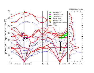
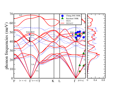
Figure 14: (Adapted from floris11 ; color online) Phonon dispersion and vibrational DOS of MnO (top) and NiO (bottom), calculated with GGA (dashed blue lines) and GGA+U (thick solid red lines). Blue (black) arrows mark the GGA+U (GGA) magnetic splittings and their sign. Upper plot: filled symbols represent experimental data chung03 ; rudolf08 ; haywood71 , and open symbols the results from other calculations (at zone center) massidda99 . Lower plot: symbols represent experimental data chung03 ; reichardt75 .

Fig. 14 compares the vibrational spectrum of MnO and NiO obtained with GGA and GGA+U. As evident from the figure, the Hubbard correction produces an overall increase in the phonon frequencies of both materials, significantly improving the agreement with available experimental results chung03 ; rudolf08 ; haywood71 ; reichardt75 . In particular, it recovers the agreement for the TO and LO modes, strongly underestimated ($\approx$ 15 meV) by GGA. The phonon frequencies computed from the GGA+U ground state lead to a reduced splitting between TO modes compared to GGA, which is also in better agreement with experimental data.

These results demonstrate that electronic correlations have significant effects on the structural and vibrational properties and that the calculation of quantities involving phonons and their interaction with other excitations (e.g., Raman spectra or electron-phonon couplings) or requiring the integration of the vibrational frequencies across the Brillouin zone (e.g., to account for finite ionic temperature effects) must employ corrective functionals accounting for strong correlation.

VII.4 Derivatives of U

In all the previuos sections, while discussing the contribution of the Hubbard functional to energy derivatives, the Hubbard $U$ was kept fixed. In fact, its dependence on the atomic positions and/or the cell parameters is usually assumed to be small and neglected. This is, of course, an approximation, whose validity should be tested carefully, case by case. In fact, some recent works have shown that accounting for the variation of $U$ with the ionic positions and with lattice parameters can be important to obtain quantitatively predictive results. In Ref. hsu09 , focused on the properties of the low-spin ground state of LaCoO₃ under pressure, the Hubbard $U$ was recalculated for every volume explored. This structurally-consistent $U$ proved to be crucial to predict the value of pressure-dependent structural parameters (such as, lattice spacing, rhombohedral angle, Co-O distance and bond angles) in good agreement with experimental data. In Ref. tsuchiya06 the linear-response calculation of the $U$ as a function of the unit cell volume (or the applied pressure) allowed for a precise evaluation of the pressure-induced high-spin to low-spin transition in (Mg_1-xFe_x)O Magnesiowüstite for different Fe concentrations.

The complexity of the analytic expression of the Hubbard $U$ makes it difficult to account for its variation with the atomic position and lattice parameters. However, a recent article kulik11 has introduced a method to efficiently compute the derivative $dU^{I}/dR^{J}$ that allows to capture (at least at first order) the variation of $U$ with the ionic position. This extension is based on the linear-response approach to compute $U$ cococcioni05 discussed in section III. Starting from Eq. 27, it is easy to work out the formal expression of the derivative of the Hubbard $U$ with respect to the atomic positions (atomic and direction indexes are dropped for simplicity):

$$\frac{dU}{d{\bf\rm\tau}}=\frac{d}{d{\bf\rm\tau}}\left(\chi_{0}^{-1}-\chi^{-1}\right)=\chi^{-2}\frac{d\chi}{d{\bf\rm\tau}}-\chi_{0}^{-2}\frac{d\chi_{0}}{d{\bf\rm\tau}}.$$ (63)

The derivative of the respose functions can be also evaluated starting from their definition:

$$\frac{d\chi}{d{\bf\rm\tau}}=\frac{d}{d{\bf\rm\tau}}\frac{dn}{d\alpha}=\frac{d}{d\alpha}\frac{dn}{d{\bf\rm\tau}}\approx\frac{d}{d\alpha}\frac{\partial n}{\partial{\bf\rm\tau}}.$$ (64)

The approximation made in the last equality of this expression allows to use the “bare” derivative of the atomic occupations to compute the derivative of the response matrices. This is the quantity used in the calculation of the Hubbard forces and expressed in Eq. 49. In practice, the derivative of the response matrices $\chi$ and $\chi_{0}$ can be obtained from the same linear response calculation used to compute their values, evaluating the response of the derivative of the atomic occupations (Eq. 49) to the perturbation added to the potential, Eq. 22 (refer to Ref. kulik11 for details). In Ref. kulik11 this approach is used to account for the variation of $U$ with atomic positions during chemical reactions involving bi-atomic molecules. It is demonstrated that a configuration-dependent effective interaction parameter significantly improves the quantitative description of the potential energy surfaces the system explores with respect to calculations (quite common in literature) using the same (average) value of $U$ for all the configurations.

The promising results obtained in Ref. kulik11 give hope that analogous implementations could actually be used to estimate the dependence of $U$ on the strain of a crystal, $dU^{I}/d\epsilon_{\alpha\beta}$, (analogous formulas apply) to be used in the calculation of the stress, and also to compute the contribution to second derivatives. If the derivatives of the Hubbard $U$ could be evaluated automatically (possibly from the expression of the effective interaction in terms of atomic orbitals) its inclusion in calculations would greatly improve the accuracy of molecular dynamics simulations based on LDA+U sit06 ; sit07 .

VIII Summary and outlook

Based on a simple corrective functional modeled on the Hubbard Hamiltonian, the LDA+U method is one of the most widely used computational approaches to correct the inaccuracies of approximate DFT exchange correlation functionals in the description of systems characterized by strongly correlated (and typically localized) electrons. Much of the popularity this method has gained in the scientific community employing DFT as main computational tool is certainly related to the fact that it is straightforward to implement in existing DFT codes, is very simple to use, and carries a very marginal additional computational cost with respect to “standard” functionals. These features, together with the possibility to tune the strength of the Hubbard correction through the numerical value of a single, easy-to-control interaction parameter, have contributed to establish LDA+U as a semiemprical method, or as a tool for a rough (and mostly qualitative) assessment of the effects of electronic correlation on the physical properties of a given system. As a consequence, LDA+U has often been regarded as a semiquantitative approach (as is the Hubbard model it is based on) or, at most, as a first order correction to approximate DFT functionals to provide a starting point for more sophisticated and supposedly more accurate approaches.

In this article we have discussed the LDA+U method with the aim to assess its potential and to clarify the conditions under which it can be expected to provide a quantitative description of correlated materials. The analysis was based on the review of the theoretical foundation of this method, a description of its most common formulations and implementations, and a discussion of its framing in the context of DFT, highlighting the typical problems it aims to address, and the quality of the correction it provides. The discussion about open issues of LDA+U (e.g., the use of specific localized basis sets, the invariance of the corrective functional, the choice of the double counting term) and the illustration of the results obtained from the study of specific materials gave us the possibility to explore the descriptive potentials of this corrective approach and to remark and understand its limits. Through a review of the existing literature it was shown, for example, how LDA+U improves the evaluation of the band gap of insulators, the description of the structural and magnetic properties of correlated systems, the energetics of electron transfer processes and chemical reactions. We also pointed out many difficulties this method encounters in describing the properties of metals or, in general, systems with more delocalized electrons. Particular emphasis was put on the necessity to have a method to compute the effective electronic interactions from first principles. A linear response approach to this problem was described in detail and compared with other methods present in literature. Recent extensions to the formulation of the Hubbard corrective functional were then presented, along with the beneficial effects they have on the accuracy of LDA+U and on the range of systems and phenomena that can be reliably modeled by this method. In particular, it was shown that the inclusion of inter-site Coulomb interactions in the Hubbard corrective functional enables the description of systems where electronic localization occurs on hybridized orbitals or for which excitations from the ground state may be accompanied by electron-transfer processes. At the same time, the extension of the Hubbard corrective Hamiltonian to explicitly include magnetic (Hund’s rule) couplings was discussed highlighting the very significant improvements it brings to the treatment of materials where the onset of a magnetic ground state favors or competes with electronic localization or where spin and charge degrees of freedom are intimately coupled in determining the physical behavior of electrons on strongly localized orbitals. Finally, it was shown that the possibility to easily define and implement energy derivatives of the corrective functional renders LDA+U a quite unique tool to capture the effects of electronic correlation and Coulomb-driven localization on the structural properties of materials (such as, e.g., equilibrium lattice parameters, elastic constants, etc), to perform molecular dynamics simulations, to compute the vibrational spectrum and related quantities (Raman spectra, electron-phonon couplings, etc).

Notwithstanding the inherent limits of this approach (such as, e.g., its static character and the consequent inability to capture dynamical, frequency dependent effects), we argue that LDA+U represents a very useful computational tool to model correlated systems that, while significantly improving the accuracy of approximate DFT energy functionals, presents marginal computational costs, thus enabling the possibility of calculations that would be impossible or overly expensive if based on a more accurate description of the quantum many-body features of the electronic ground state.

LDA+U can provide quantitatively precise predictions about the physical beavior of various systems, provided the appropriate formulation of the corrective functional is used and the effective electronic interactions are precisely computed for all the atomic sites the Hubbard correction acts on. Further extensions and refinements to the Hubbard corrective functional are however highly desirable to improve the accuracy and the numerical efficiency of the LDA+U method. The automatic calculation of the effective electronic interactions (e.g., using the expression in Eq. (III.3.2)) would certainly represent a useful extension to current implementations as it would avoid the need of separate (e.g., linear-response) calculations to achieve this result, and would allow to account for the variation of the electronic couplings with the atomic positions, the magnetic configuration, and the physical conditions the material is subject to. A more flexile expression of the corrective functional (including, e.g., selected multi-site and multi-orbital interaction terms of the Hubbard Hamiltonian) would be also very important to improve its descriptive capability and its numerical accuracy, as demonstrated already by the definition of the LDA+U+V and the LDA+U+J approaches. Extensions of this kind require, however, a very substantial theoretical work that should identify: $i)$ the precise conditions under which the mean-field-like Hubbard functional of LDA+U can be expected to contribute the necessary corrections for a precise representation of the many-body features of electronic interactions; $ii)$ the extensions to the expression of the corrective functional necessary to make it work effectively in more general cases (e.g., metals, paramagnetic insulators, etc). We hope that this work will be completed in the near future and will result in the definition of a generalized corrective functional able to describe degenerate ground states of correlated systems without breaking/lowering the symmetry of the electronic charge density, to automatically distinguish genuine metallic ground states from the overlap of degenerate insulating solutions, and to describe the main effects of possible interplays between charge and spin degrees of freedom.

IX Acknowledgements

Authors would like to thank Dr. S. Fabris and Dr. K. Yang for providing figures 2 and 6 respectively. M. C. acknowledges support from the NSF CAREER award, DMR 1151738.

Appendix A Linear response calculation of U

In this appendix linear-response theory will be used to derive the explicit expression of the Hubbard $U$, as computed in Eq. (27). To this purpose it is useful to start from a generalization of the perturbing potential in Eq. (22) that is based on a non-diagonal projector operator:

$$\Delta V_{ext}^{IJ}=\alpha^{IJ}_{ij}|\phi^{I}_{i}\rangle\langle\phi^{J}_{j}|$$ (65)

where the upper and lower case letters label atomic sites and electronic states, respectively. In linear response-theory the variation of a (Kohn-Sham) wave function can be computed as follows (comprehensive indexes $m$ and $n$ are understood to run over k-points and bands while spin is omitted for simplicity):

$$\Delta\psi_{n}=\sum_{m\neq n}\psi_{m}\frac{\langle\psi_{m}|\Delta V_{scf}|\psi_{n}\rangle}{\epsilon_{n}-\epsilon_{m}}.$$ (66)

In this equation $\Delta V_{scf}$ is the total variation of the self-consistent potential containing, besides $\Delta V_{ext}$, a term originating from the response of the electronic system that reads:

$$\Delta{\hat{V}}_{\rm resp}({\rm\bf r})=\left(\Delta V_{H}({\rm\bf r})+\Delta V_{\rm xc}({\rm\bf r})\right)\ {\hat{K}}({\rm\bf r})\,\,\,,\,\,\,$$ (67)

where ${\hat{K}}({\rm\bf r})=|{\rm\bf r}\rangle\langle{\rm\bf r}|$ and

$$\Delta V_{H}({\rm\bf r})=\int\frac{\Delta\rho({\rm\bf r}^{\prime})}{|{\rm\bf r}-{\rm\bf r}^{\prime}|}d{\rm\bf r}^{\prime}\,\,\,,\,\,\,$$

$$\Delta V_{\rm xc}({\rm\bf r})=\int\frac{\delta v_{\rm xc}({\rm\bf r})}{\delta\rho({\rm\bf r}^{\prime})}\,\Delta\rho({\rm\bf r}^{\prime})d{\rm\bf r}^{\prime}.$$ (68)

To proceed we will assume that the atomic basis set $\{\phi^{I}_{i}\}$ is orthogonal and complete. Therefore the identity can be resolved as:

$$\mathbf{1}=\sum_{Ii}|\phi^{I}_{i}\rangle\langle\phi^{I}_{i}|.$$ (69)

Also, a generalized occupation matrix, analogous to the one defined in Eq. (42), is needed:

$$n^{IJ}_{ij}=\sum_{n}f_{n}\langle\phi_{i}^{I}|\psi_{n}\rangle\langle\psi_{n}|\phi_{j}^{J}\rangle.$$ (70)

For the sake of simplicity, the spin index is dropped for KS states (or can be considered included in their comprehensive index $n$). The $f_{n}$ coefficients represent the occupations of the KS states (determined from the Fermi-Dirac distribution of the corresponding eigenvalues around the Fermi energy). in this part only the case of semiconductors/insulators will be discussed (metals would require to explicitly account for the response of the $f_{n}$, as shown, e.g., in Ref. baroni01 ). Using Eq. (66) the response of the occupation matrix to the external perturbation can be expressed as follows:

$$\Delta n^{IJ}_{ij} = \sum_{n}f_{n}\left[\langle\psi_{n}|\phi_{j}^{J}\rangle\langle\phi_{i}^{I}|\Delta\psi_{n}\rangle+\langle\Delta\psi_{n}|\phi_{j}^{J}\rangle\langle\phi_{i}^{I}|\psi_{n}\rangle\right]$$ (71)

$$= 2~{}Re\sum_{n\in{\rm v}}\sum_{m\in{\rm c}}\frac{\langle\phi_{i}^{I}|\psi_{m}\rangle\langle\psi_{m}|\Delta V_{scf}|\psi_{n}\rangle\langle\psi_{n}|\phi_{j}^{J}\rangle}{\epsilon_{n}-\epsilon_{m}}.$$

The last equality is a consequence of the fact that only the case of semiconductors/insulators is discussed in this part (metals would require to explicitly account for the response of the $f_{n}$, as shown, e.g., in Ref. baroni01 ) which allows to classify KS states as valence ($v$) or conduction ($c$) states according to their occupation ($f_{n}=1$ and $f_{n}=0$, respectively). If the system were non interacting $\Delta V_{resp}=0$, $\Delta V_{scf}=\Delta V_{ext}$. In this case the interacting and non-interacting response matrices coincide: ${\mathbf{\chi}}={\mathbf{\chi}}_{0}$. These conditions are verified if the Hartree and xc potential are the same as in the non perturbed ground state of the system (when the self-consistent solution of the KS equations has been reached) or in the perturbed calculation (which starts from the unperturbed potential and wave functions) at the very first iteration of the diagonalization process when these terms of the electron-electron interaction potential have not yet responded to the perturbation in the external potential. In fact, in these circumstances, the electronic system responds as an independent electron gas of the same density as the real one. Substituting $\Delta V_{scf}$ with $\Delta V_{ext}$ in Eq. (71), $\Delta_{0}n^{IJ}_{ij}$ is obtained. The following equalities define the response matrices (tensors) $\chi$ and $\chi_{0}$:

$$\Delta n^{IJ}_{ij} = \sum_{KLkl}(\chi_{0})^{IJLK}_{ijlk}\langle\phi_{k}^{K}|\Delta V_{scf}|\phi_{l}^{L}\rangle$$ (72)

$$= \sum_{KLkl}\chi^{IJLK}_{ijlk}\langle\phi_{k}^{K}|\Delta V_{ext}|\phi_{l}^{L}\rangle$$

$$= \sum_{KLkl}\chi^{IJLK}_{ijlk}\alpha^{KL}_{kl}$$

Based on the discussion above, the last equality can be used to evaluate $\chi_{0}$ at the first iteration of the perturbed run. From Eqs. (65), (69), (71) and (72) the following expression can be easily derived:

$$(\chi_{0})^{IJLK}_{ijlk}=2~{}Re\sum_{n\in v}\sum_{m\in c}\frac{\langle\phi_{i}^{I}|\psi_{m}\rangle\langle\psi_{n}|\phi^{J}_{j}\rangle\langle\phi^{L}_{l}|\psi_{n}\rangle\langle\psi_{m}|\phi_{k}^{K}\rangle}{\epsilon_{n}-\epsilon_{m}}.$$ (73)

In order to obtain the explicit expression of the Hubbard $U$ it is convenient to rewrite Eq. (27) in a Dyson-like form:

$$\chi=\chi_{0}+\chi_{0}~{}{\rm\mathbf{U}}~{}\chi$$ (74)

where ${\rm\mathbf{U}}$ represent the interaction matrix (tensor) of elements $U^{IJKL}_{ijkl}$. In order to compute the total response matrix $\chi$ we can use the last equality of Eq. (72):

$$\Delta n^{IJ}_{ij} = \sum_{KLkl}\chi^{IJLK}_{ijlk}\langle\phi_{k}^{K}|\Delta V_{ext}|\phi_{l}^{L}\rangle$$ (75)

$$= \sum_{KLkl}\chi^{IJLK}_{ijlk}\alpha^{KL}_{kl}.$$

Therefore, by definition, $\chi^{IJLK}_{ijlk}=\Delta n^{IJ}_{ij}/\alpha^{KL}_{kl}$ (to be understood as a finite-difference approximation of a derivative). Note the inversion in the order of indexes from $\chi$ to $\alpha$: as will be evident from the formulas below, this is required for the covariance of the theory with respect to rotations of the basis set. Using the completeness of the localized orbital basis set (Eq. (69)), it is convenient to rewrite Eq. (71) as follows:

$$\Delta n^{IJ}_{ij}=2\,~{}Re\sum_{n\in v}\sum_{m\in c}\sum_{OP}\sum_{op}\frac{\langle\psi_{n}|\phi_{j}^{J}\rangle\langle\phi_{i}^{I}|\psi_{m}\rangle\langle\psi_{m}|\phi^{O}_{o}\rangle\langle\phi^{O}_{o}|\Delta V_{scf}|\phi_{p}^{P}\rangle\langle\phi_{p}^{P}|\psi_{n}\rangle}{\epsilon_{n}-\epsilon_{m}}.$$ (76)

Using Eqs. (65) and (67) the quantity $\langle\phi^{O}_{o}|\Delta V_{scf}|\phi_{p}^{P}\rangle$ can be easily expressed as follows:

$$\langle\phi^{O}_{o}|\Delta V_{scf}|\phi_{p}^{P}\rangle=\alpha^{OP}_{op}+\langle\phi^{O}_{o}|\Delta V_{resp}|\phi_{p}^{P}\rangle=\alpha^{OP}_{op}+\int\int(\phi^{O}_{o}({\rm\bf r}))^{*}\phi_{p}^{P}({\rm\bf r})f_{Hxc}({\rm\bf r},{\rm\bf r}^{\prime})\Delta\rho({\rm\bf r}^{\prime})~{}d{\rm\bf r}~{}d{\rm\bf r}^{\prime}$$ (77)

where $f_{Hxc}$ is the Hartree and exchange-correlation interaction kernel: $f_{Hxc}({\rm\bf r},{\rm\bf r}^{\prime})=\frac{1}{|{\rm\bf r}-{\rm\bf r}^{\prime}|}+\frac{\delta v_{xc}({\rm\bf r})}{\delta\rho({\rm\bf r}^{\prime})}$. At this point we need the explicit expression of $\Delta\rho({\rm\bf r})$. Using again the completeness condition, Eq. (69), Eq. (66) can be rewritten as:

$$\Delta\psi_{n}({\rm\bf r})=\sum_{m\neq n}\sum_{Ii}\phi^{I}_{i}({\rm\bf r})\frac{\langle\phi^{I}_{i}|\psi_{m}\rangle\langle\psi_{m}|\Delta V_{scf}|\psi_{n}\rangle}{\epsilon_{n}-\epsilon_{m}}.$$ (78)

Using Eq. (76) we easily obtain:

$$\Delta\rho({\rm\bf r}) = \sum_{n}f_{n}\left[\psi_{n}^{*}({\rm\bf r})\Delta\psi_{n}({\rm\bf r})+\psi_{n}({\rm\bf r})\Delta\psi_{n}^{*}({\rm\bf r})\right]=2~{}Re\sum_{RrSs}\sum_{n\in v}\sum_{m\in c}\phi^{S}_{s}({\rm\bf r})^{*}\phi^{R}_{r}({\rm\bf r})\frac{\langle\phi^{R}_{r}|\psi_{m}\rangle\langle\psi_{n}|\phi_{s}^{S}\rangle\langle\psi_{m}|\Delta V_{scf}|\psi_{n}\rangle}{\epsilon_{n}-\epsilon_{m}}$$ (79)

$$= \sum_{RrSs}\phi^{S}_{s}({\rm\bf r})^{*}\phi^{R}_{r}({\rm\bf r})\Delta n^{RS}_{rs}=\sum_{Rr}\sum_{Ss}\sum_{KLkl}\phi^{S}_{s}({\rm\bf r})^{*}\phi^{R}_{r}({\rm\bf r})\chi^{RSLK}_{rslk}\alpha^{KL}_{kl}.$$

Inserting this expression in Eq. (77) we obtain:

$$\langle\phi^{O}_{o}|\Delta V_{scf}|\phi_{p}^{P}\rangle=\alpha^{OP}_{op}+\sum_{Rr}\sum_{Ss}\sum_{KLkl}\left[\int\int(\phi^{O}_{o}({\rm\bf r}))^{*}\phi_{p}^{P}({\rm\bf r})f_{Hxc}({\rm\bf r},{\rm\bf r}^{\prime})\phi^{S}_{s}({\rm\bf r}^{\prime})^{*}\phi^{R}_{r}({\rm\bf r}^{\prime})~{}d{\rm\bf r}~{}d{\rm\bf r}^{\prime}\right]\chi^{RSLK}_{rslk}\alpha^{KL}_{kl}.$$ (80)

Once this expression is used in Eq. (76) we finally arrive at:

$$\Delta n^{IJ}_{ij} = 2\,~{}Re\sum_{n\in v}\sum_{m\in c}\sum_{OPop}\frac{\langle\psi_{n}|\phi_{j}^{J}\rangle\langle\phi_{i}^{I}|\psi_{m}\rangle\langle\psi_{m}|\phi^{O}_{o}\rangle\langle\phi_{p}^{P}|\psi_{n}\rangle}{\epsilon_{n}-\epsilon_{m}}\alpha^{OP}_{op}$$ (81)

$$+ 2\,~{}Re\sum_{n\in v}\sum_{m\in c}\sum_{OPop}\sum_{RSrs}\sum_{KLkl}\frac{\langle\psi_{n}|\phi_{j}^{J}\rangle\langle\phi_{i}^{I}|\psi_{m}\rangle\langle\psi_{m}|\phi^{O}_{o}\rangle\langle\phi_{p}^{P}|\psi_{n}\rangle}{\epsilon_{n}-\epsilon_{m}}\times$$

$$\times \left[\int\int(\phi^{O}_{o}({\rm\bf r}))^{*}\phi_{p}^{P}({\rm\bf r})f_{Hxc}({\rm\bf r},{\rm\bf r}^{\prime})\phi^{S}_{s}({\rm\bf r}^{\prime})^{*}\phi^{R}_{r}({\rm\bf r}^{\prime})~{}d{\rm\bf r}~{}d{\rm\bf r}^{\prime}\right]\chi^{RSLK}_{rslk}\alpha^{KL}_{kl}.$$

Taking the derivative of both members with respect to $\alpha^{KL}_{kl}$ and using Eq. (73), the following Dyson-like expression is finally arrived at:

$$\chi^{IJLK}_{ijlk}=(\chi_{0})^{IJLK}_{ijlk}+\sum_{OPop}\sum_{RSrs}(\chi_{0})^{IJPO}_{ijpo}\left[\int\int(\phi^{O}_{o}({\rm\bf r}))^{*}\phi_{p}^{P}({\rm\bf r})f_{Hxc}({\rm\bf r},{\rm\bf r}^{\prime})\phi^{S}_{s}({\rm\bf r}^{\prime})^{*}\phi^{R}_{r}({\rm\bf r}^{\prime})~{}d{\rm\bf r}~{}d{\rm\bf r}^{\prime}\right]\chi^{RSLK}_{rslk}.$$ (82)

Direct comparison with Eq. (74) yields:

$$U^{OPSR}_{opsr}=\int\int(\phi^{O}_{o}({\rm\bf r}))^{*}\phi_{p}^{P}({\rm\bf r})\left[\frac{1}{|{\rm\bf r}-{\rm\bf r}^{\prime}|}+\frac{\delta v_{xc}({\rm\bf r})}{\delta\rho({\rm\bf r}^{\prime})}\right]\phi^{S}_{s}({\rm\bf r}^{\prime})^{*}\phi^{R}_{r}({\rm\bf r}^{\prime})~{}d{\rm\bf r}~{}d{\rm\bf r}^{\prime}$$ (83)

which is the central result of this appendix. Eq. (83) highlights that the effective interaction computed through the linear response approach illustrated above is nothing else than the expectation value of the $bare$ Hartree and xc kernels on quadruplets of wave functions belonging to the chosen basis set (e.g., orthogonalized atomic orbitals).

In the linear-response calculation of $U$ introduced in Ref. cococcioni05 the perturbation is applied uniformly to all the localized orbitals of the same atom:

$$\Delta V_{ext}^{I}=\alpha^{I}\sum_{i}|\phi_{i}^{I}\rangle\langle\phi^{I}_{i}|$$ (84)

and the response of the system is studied through the variations of the trace of the occupation matrix on each site:

$$\Delta n^{I}=\sum_{i}\Delta n_{ii}^{II}=\sum_{i}\sum_{Rr}\chi^{IIRR}_{iirr}\alpha_{rr}^{RR}=\sum_{R}\alpha^{R}\sum_{ir}\chi^{IIRR}_{iirr}.$$ (85)

In Eq. (85) the last equality is justified by the fact that in the procedure illustrated in Ref. cococcioni05 the strength of the perturbation is uniform over all the states of the same atoms. The response matrix computed by the procedure in Ref. cococcioni05 can thus be expressed as:

$$\tilde{\chi}^{IR}=\sum_{ir}\chi^{IIRR}_{iirr}$$ (86)

and, from Eq. (82), the following equation easily follows:

$$\tilde{\chi}^{IR} = \tilde{\chi}^{IR}_{0}+\sum_{ir}\sum_{KQTZ}\sum_{kqtz}\left(\chi_{0}\right)^{IIQK}_{iiqk}U^{KQTZ}_{kqtz}\chi^{ZTRR}_{ztrr}$$ (87)

$$\equiv \tilde{\chi}^{IR}_{0}+\tilde{\chi}^{IQ}_{0}\tilde{U}^{QZ}\tilde{\chi}^{ZR}\equiv\tilde{\chi}^{IR}_{0}+A^{IR}$$

(repeated indexes are summed over). Unfortunately, Eq. (87) is not closed in $\tilde{\chi}$ and $\tilde{\chi}_{0}$ and the last two equalities (second line) define the quantities $\tilde{\rm\bf U}$ and ${\rm\bf A}$. The computed Hubbard $U$ thus results:

$$\tilde{U}^{QZ}=(\tilde{\chi}_{0}^{-1})^{QR}A^{RS}(\tilde{\chi}^{-1})^{SZ}=\sum_{RS}(\tilde{\chi}_{0}^{-1})^{QR}\left[\sum_{rs}\sum_{KSTM}\sum_{kstm}\left(\chi_{0}\right)^{RRSK}_{rrsk}U^{KSTM}_{kstm}\chi^{MTSS}_{mtss}\right](\tilde{\chi}^{-1})^{SZ}.$$ (88)

In matrix notation this equation can be expressed as:

$$\tilde{\rm\bf U}=({\rm\bf\tilde{\chi}_{0}})^{-1}{\rm\bf A}~{}{\rm\bf\tilde{\chi}}^{-1}.$$ (89)

From the definition given in Eq. (87) we also have:

$$\tilde{\rm\bf U}=({\rm\bf\tilde{\chi}_{0}})^{-1}-{\rm\bf\tilde{\chi}}^{-1}$$ (90)

Combining this equation with Eq. (89) to eliminate $\tilde{\chi}^{-1}$ we obtain:

$$\tilde{\rm\bf U} = (\tilde{\chi}_{0})^{-1}{\rm\bf A}((\tilde{\chi}_{0})^{-1}-\tilde{\rm\bf U})$$ (91)

$$= (\tilde{\chi}_{0})^{-1}{\rm\bf A}(\tilde{\chi}_{0})^{-1}-(\tilde{\chi}_{0})^{-1}{\rm\bf A}\tilde{\rm\bf U}$$

from which, solving for $\tilde{\rm\bf U}$, gives:

$$\tilde{\rm\bf U}=\frac{(\tilde{\chi}_{0})^{-1}{\rm\bf A}(\tilde{\chi}_{0})^{-1}}{1+(\tilde{\chi}_{0})^{-1}{\rm\bf A}}$$ (92)

that shows a formal resemblance to the effective interaction, Eq. (21), computed from cRPA. A more detailed discussion on the comparison between linear-response and cRPA results is offered in the article, after Eq. (33). Notice that, with respect to the notation of section III, the meaning of quantities with and without “$~{}\tilde{}~{}$” is reversed; for example, there $\tilde{U}$ indicated the fully orbital dependent interaction parameter, here it represents the atomically averaged (and orbital independent) one obtained from actual linear response calculations.

In order to understand how the unscreened interaction $U^{KSTM}_{kstm}$, whose value is typically in the 15-30 eV range, is screened to an effective $\tilde{U}^{QZ}$ in the 2-6 eV range, it is appropriate to analyze the expression in Eq. (88). To this purpose it is useful to separate in the response matrices a site- and state- “bi-diagonal” term from off-diagonal ones as follows:

$$\chi^{ZTSS}_{ztss}=\delta_{tz}\delta_{TZ}\chi^{TTSS}_{ttss}+\bar{\chi}^{ZTSS}_{ztss}$$ (93)

(the same decomposition is assumed for $\chi_{0}$). Assuming the dominance of diagonal terms over off-diagonal ones in the occupation matrices, it is fair to deduce that $\bar{\chi}$ is small with respect to the diagonal terms. Also, due to the fact that the increase in the diagonal parts of the occupation matrices usually decreases off-diagonal ones, the two terms of the right hand side of Eq. (93) generally have opposite signs. Inserting Eq. (93) in Eq. (88) one easily obtains:

$$\tilde{U}^{QZ} = \sum_{RS}(\tilde{\chi}_{0}^{-1})^{QR}\left[\sum_{rs}\sum_{KT}\sum_{kt}\left(\chi_{0}\right)^{RRKK}_{rrkk}U^{KKTT}_{kktt}\chi^{TTSS}_{ttss}\right](\tilde{\chi}^{-1})^{SZ}$$ (94)

$$+ \sum_{RS}(\tilde{\chi}_{0}^{-1})^{QR}\left[\sum_{rs}\sum_{KSTM}\sum_{kstm}\left(\bar{\chi}_{0}\right)^{RRSK}_{rrsk}U^{KSTM}_{kstm}\chi^{MTSS}_{mtss}\right](\tilde{\chi}^{-1})^{SZ}$$

$$+ \sum_{RS}(\tilde{\chi}_{0}^{-1})^{QR}\left[\sum_{rs}\sum_{KSTM}\sum_{kstm}\left(\chi_{0}\right)^{RRSK}_{rrsk}U^{KSTM}_{kstm}\bar{\chi}^{MTSS}_{mtss}\right](\tilde{\chi}^{-1})^{SZ}+\mathcal{O}(\bar{\chi}_{0}\bar{\chi}).$$

If the unscreened interaction can be safely approximated by its atomic average, $U^{KKTT}_{kktt}\sim\bar{U}^{KKTT}$, Eq. (94) becomes:

$$\tilde{U}^{QZ} = \bar{U}^{QZ}+\sum_{RS}(\tilde{\chi}_{0}^{-1})^{QR}\left[\sum_{rs}\sum_{KSTM}\sum_{kstm}\left(\bar{\chi}_{0}\right)^{RRSK}_{rrsk}U^{KSTM}_{kstm}\chi^{MTSS}_{mtss}\right](\tilde{\chi}^{-1})^{SZ}$$ (95)

$$+ \sum_{RS}(\tilde{\chi}_{0}^{-1})^{QR}\left[\sum_{rs}\sum_{KSTM}\sum_{kstm}\left(\chi_{0}\right)^{RRSK}_{rrsk}U^{KSTM}_{kstm}\bar{\chi}^{MTSS}_{mtss}\right](\tilde{\chi}^{-1})^{SZ}+\mathcal{O}(\bar{\chi}_{0}\bar{\chi}).$$

As explained above, the second and third terms on the r.h.s. of Eq. (95) are negative (and dominant on the last) and are responsible for the significant difference in value between $\tilde{U}^{QZ}$ and $\bar{U}^{QZ}$.

References

- (1) P. Hohenberg and W. Kohn. Inhomogeneous Electron Gas. Phys. Rev., 136(3B):B864–B871, 1964.
- (2) W. Kohn and L. J. Sham. Self-Consistent Equations Including Exchange and Correlation Effects. Phys. Rev., 140(4A):A1133–A1138, 1965.
- (3) I. G. Austin and N. F. Mott. Metallic and Nonmetallic Behavior in Transition Metal Oxides. Science, 168:71, 1970.
- (4) W. Metzner and D. Vollhardt. Correlated Lattice Fermions in d= Dimensions. Phys. Rev. Lett., 62(3):324–327, 1989.
- (5) E. Muller-Hartmann. Correlated fermions on a lattice in high dimensions. Z. Phys. B: Condens. Matter, 74:507, 1989.
- (6) U. Brandt and C. Mielsch. Thermodynamics and correlation functions of the Falicov-Kimball model in large dimensions. Z. Phys. B: Condens. Matter, 75:365, 1989.
- (7) V. Janis. A new construction of thermodynamic mean-field theories of itinerant fermions: application to the Falicov-Kimball model. Z. Phys. B: Condens. Matter, 83:227, 1991.
- (8) A. Georges and G. Kotliar. Hubbard model in infinite dimensions. Phys. Rev. B, 45(12):6479–6483, 1992.
- (9) A. Georges, G. Kotliar, W. Krauth, and M. J. Rozenberg. Dynamical mean-field theory of strongly correlated fermion systems and the limit of infinite dimensions. Rev. Mod. Phys., 68(1):13, 1996.
- (10) E. Pavarini, E. Koch, D. Vollhardt, and A. Lichtenstein, editors. The LDA+DMFT approach to strongly correlated materials. Forschungszentrum, Julich, 2011. Available from: http://juwel.fz-juelich.de:8080/dspace/handle/2128/4467.
- (11) W. Yang, Y. Zhang, and P. W. Ayers. Degenerate Ground States and a Fractional Number of Electrons in Density and Reduced Density Matrix Functional Theory. Phys. Rev. Lett., 84(22):5172, 2000.
- (12) N. Helbig, N. N. Lathiotakis, M. Albrecht, and E. K. U. Gross. Discontinuity of the chemical potential in reduced-density-matrix-functional theory. Europhysics Lett., 77:67003, 2007.
- (13) R. Requist and O. Pankratov. Generalized Kohn-Sham system in one-matrix functional theory. Phys. Rev. B, 77:235121, 2008.
- (14) S. Sharma, J. K. Dewhurst, N. N. Lathiotakis, and E. K. U. Gross. Reduced density matrix functional for many-electron systems. Phys. Rev. B, 78(20):201103, 2008.
- (15) N. Helbig, N. N. Lathiotakis, and E. K. U. Gross. Discontinuity of the chemical potential in reduced-density-matrix-functional theory for open-shell systems. Phys. Rev. A, 79(2):022504, 2009.
- (16) K. Capelle and V. Leiria Campo Jr. Density functionals and model Hamiltonians: Pillars of many-particle physics. Physics Reports, 528(3):91–159, 2013.
- (17) V. I. Anisimov and O. Gunnarsson. Density-functional calculation of effective Coulomb interactions in metals. Phys. Rev. B, 43(10):7570–7574, 1991.
- (18) V. I. Anisimov, J. Zaanen, and O. K. Andersen. Band theory and Mott insulators: Hubbard U instead of Stoner I. Phys. Rev. B, 44(3):943–954, 1991.
- (19) V. I. Anisimov, I. V. Solovyev, M. A. Korotin, M. T. Czyżyk, and G. A. Sawatzky. Density-functional theory and NiO photoemission spectra. Phys. Rev. B, 48:16929–16934, 1993.
- (20) I. V. Solovyev, P. H. Dederichs, and V. I. Anisimov. Corrected atomic limit in the local-density approximation and the electronic structure of d impurities in Rb. Phys. Rev. B, 50:16861, 1994.
- (21) V. I. Anisimov, F. Aryasetiawan, and A. I. Lichtenstein. First-principles calculations of the electronic structure and spectra of strongly correlated systems: the LDA + U method. J. Phys.: Cond. Matter, 9(4):767, 1997.
- (22) S. Wang, Z. Wang, W. Setyawan, N. Mingo, and S. Curtarolo. Assessing the Thermoelectric Properties of Sintered Compounds via High-Throughput Ab-Initio Calculations. Phys. Rev. X, 1:021012, 2011.
- (23) K. Yang, W. Setyawan, S. Wang, M. Buongiorno Nardelli, and S. Curtarolo. A search model for topological insulators with high-throughput robustness descriptors. Nat. Mat., 11:614–619, 2012.
- (24) S. Curtarolo, G. L. W. Hart, M. Buongiorno Nardelli, N. Mingo, S. Sanvito, and O. Levy. The high-throughput highway to computational materials design. Nat. Mat., 12:191–201, 2013.
- (25) M. Cococcioni. Accurate and efficient calculations on strongly correlated minerals with the LDA+U method; review and perspectives. Reviews in Mineralogy and Geochemistry, 71:147–167, 2010.
- (26) P. H.-L. Sit, M. Cococcioni, and N. Marzari. Realistic, quantitative descriptions of electron-transfer reactions: diabatic surfaces from first-principles molecular dynamics. Phys. Rev. Lett., 97(2):028303, 2006.
- (27) P. H.-L. Sit, M. Cococcioni, and N. Marzari. Car-Parrinello molecular dynamics in the DFT+U formalism: Structure and energetics of solvated ferrous and ferric ions. J. Electroanalytical Chem., 607:107, 2007.
- (28) A. Floris, S. de Gironcoli, E. K. U. Gross, and M. Cococcioni. Vibrational properties of MnO and NiO from DFT+U-based Density Functional Perturbation Theory. Phys. Rev. B, 84:161102(R), 2011.
- (29) H. Hsu, P. Blaha, M. Cococcioni, and R. M. Wentzcovitch. Spin-State Crossover and Hyperfine Interactions of Ferric Iron in MgSiO3 Perovskite. Phys. Rev. Lett., 106(11):118501, 2011.
- (30) J. Hubbard. Electron Correlations in Narrow Energy Bands. Proc. Roy. Soc. Lond. A, 276:238, 1963.
- (31) J. Hubbard. Electron Correlations in Narrow Energy Bands. II. The Degenerate Band Case. Proc. Roy. Soc. Lond. A, 277:237, 1964.
- (32) J. Hubbard. Electron Correlations in Narrow Energy Bands. III. An Improved Solution . Proc. Roy. Soc. Lond. A, 281:401, 1964.
- (33) J. Hubbard. Electron Correlations in Narrow Energy Bands. IV. The Atomic Representation. Proc. Roy. Soc. Lond. A, 285:542, 1965.
- (34) J. Hubbard. Electron Correlations in Narrow Energy Bands. V. A Perturbation Expansion About the Atomic Limit. Proc. Roy. Soc. Lond. A, 296:82, 1967.
- (35) J. Hubbard. Electron Correlations in Narrow Energy Bands. VI. The Connexion with Many-Body Perturbation Theory. Proc. Roy. Soc. Lond. A, 296:100, 1967.
- (36) M. T. Czyżyk and G. A. Sawatzky. Local-density functional and on-site correlations: The electronic structure of La2CuO4 and LaCuO3. Phys. Rev. B, 49(20):14211–14228, 1994.
- (37) A. G. Petukhov, I. I. Mazin, L. Chioncel, and A. I. Lichtenstein. Correlated metals and the method. Phys. Rev. B, 67(15):153106, 2003.
- (38) V. I. Anisimov, A. V. Kozhevnikov, M. A. Korotin, A. V. Lukoyanov, and D. A. Khafizullin. Orbital density functional as a means to restore the discontinuities in the total-energy derivative and the exchange-correlation potential. J. of Phys.: Condens. Matter, 19(10):106206, 2007.
- (39) A. I. Liechtenstein, V. I. Anisimov, and J. Zaanen. Density-functional theory and strong interactions: Orbital ordering in Mott-Hubbard insulators. Phys. Rev. B, 52(8):R5467–R5470, 1995.
- (40) S. L. Dudarev, G. A. Botton, S. Y. Savrasov, C. J. Humphreys, and A. P. Sutton. Electron-energy-loss spectra and the structural stability of nickel oxide: An LSDA+U study. Phys. Rev. B, 57(3):1505–1509, 1998.
- (41) David D. O’Regan, Mike C. Payne, and Arash A. Mostofi. Subspace representations in ab initio methods for strongly correlated systems. Phys. Rev. B, 83:245124, 2011.
- (42) M. J. Han, T. Ozaki, and J. Yu. electronic structure calculation method based on the nonorthogonal pseudoatomic orbital basis. Phys. Rev. B, 73:045110, 2006.
- (43) David D. O’Regan, Nicholas D. M. Hine, Mike C. Payne, and Arash A. Mostofi. Projector self-consistent using nonorthogonal generalized Wannier functions. Phys. Rev. B, 82:081102, 2010.
- (44) J. P. Perdew, R. G. Parr, M. Levy, and J. L. Baldus Jr. Density-Functional Theory for Fractional Particle Number: Derivative Discontinuity of the Energy. Phys. Rev. Lett., 49(23):1961, 1982.
- (45) J. P. Perdew and M. Levy. Physical Content of the Exact Kohn-Sham Orbital Energies: Band Gaps and Derivative Discontinuities. Phys. Rev. Lett., 51(20):1884–1887, 1983.
- (46) R. W. Godby, M. Schlüter, and L. J. Sham. Accurate Exchange-Correlation Potential for Silicon and Its Discontinuity on Addition of an Electron. Phys. Rev. Lett., 56(22):2415–2418, 1986.
- (47) M. Cococcioni and S. de Gironcoli. Linear response approach to the calculation of the effective interaction parameters in the method. Phys. Rev. B, 71(3):035105, 2005.
- (48) S. Fabris, S. de Gironcoli, S. Baroni, G. Vicario, and G. Balducci. Taming multiple valency with density functionals: A case study of defective ceria. Phys. Rev. B, 71:041102, 2005.
- (49) S. Fabris, G. Vicario, G. Balducci, S. de Gironcoli, and S. Baroni. Electronic and Atomistic Structures of Clean and Reduced Ceria Surfaces. The Journal of Physical Chemistry B, 109(48):22860–22867, 2005.
- (50) C. Di Valentin, G. Pacchioni, and A. Selloni. Reduced and n-Type Doped TiO2: Nature of Ti3+ Species. J. Phys. Chem. C, 113(48):20543–20552, 2009.
- (51) E. Finazzi, C. Di Valentin, G. Pacchioni, and A. Selloni. Excess electron states in reduced bulk anatase TiO2: Comparison of standard GGA, GGA + U, and hybrid DFT calculations. J. Chem. Phys., 129(15):154113, 2008.
- (52) G. Mattioli, P. Alippi, F. Filippone, R. Caminiti, and A. Amore Bonapasta. Deep versus Shallow Behavior of Intrinsic Defects in Rutile and Anatase TiO2 Polymorphs. J. Phys. Chem. C, 114(49):21694–21704, 2010.
- (53) L. Vaugier, H. Jiang, and S. Biermann. Hubbard and Hund exchange in transition metal oxides: Screening versus localization trends from constrained random phase approximation. Phys. Rev. B, 86:165105, 2012.
- (54) E. Bousquet and N. Spaldin. dependence in the treatment of noncollinear magnets. Phys. Rev. B, 82:220402, 2010.
- (55) T. Jeong and W. E. Pickett. First-principles study of the electronic structure of heavy fermion YbRh2Si2. Journal of Physics: Condensed Matter, 18(27):6289, 2006.
- (56) L. de’ Medici. Hund’s coupling and its key role in tuning multiorbital correlations. Phys. Rev. B, 83:205112, 2011.
- (57) L. de’ Medici, J. Mravlje, and A. Georges. Janus-Faced Influence of Hund’s Rule Coupling in Strongly Correlated Materials. Phys. Rev. Lett., 107:256401, 2011.
- (58) F. Bultmark, F. Cricchio, O. Grånäs, and L. Nordström. Multipole decomposition of energy and its application to actinide compounds. Phys. Rev. B, 80:035121, 2009.
- (59) H. Nakamura, N. Hayashi, N. Nakai, M. Okumura, and M. Machida. First-principle electronic structure calculations for magnetic moment in iron-based superconductors: An LSDA + negative study. Physica C: Superconductivity, 469(15–20):908 – 911, 2009.
- (60) E. R. Ylvisaker, W. E. Pickett, and K. Koepernik. Anisotropy and magnetism in the method. Phys. Rev. B, 79(3):035103, 2009.
- (61) Xiao-Bing Feng and N. M. Harrison. Metal-insulator and magnetic transition of NiO at high pressures. Phys. Rev. B, 69(3):035114, 2004.
- (62) T. Körzdörfer and N. Marom. Strategy for finding a reliable starting point for demonstrated for molecules. Phys. Rev. B, 86:041110, 2012.
- (63) O. Bengone, M. Alouani, P. Blöchl, and J. Hugel. Implementation of the projector augmented-wave LDA+U method: Application to the electronic structure of NiO. Phys. Rev. B, 62(24):16392–16401, 2000.
- (64) I. de P. R. Moreira, F. Illas, and R. L. Martin. Effect of Fock exchange on the electronic structure and magnetic coupling in NiO. Phys. Rev. B, 65(15):155102, 2002.
- (65) M. D. Towler, N. L. Allan, N. M. Harrison, V. R. Saunders, W. C. Mackrodt, and E. Aprà. Ab initio study of MnO and NiO. Phys. Rev. B, 50:5041–5054, 1994.
- (66) R. M. Dreizler and E. K. U. Gross. Density Functional Theory: An Approach to the Quantum Many-Body Problem. Springer-Verlag, Berlin, Heidelber, New York.
- (67) M. K. Y. Chan and G. Ceder. Efficient Band Gap Prediction for Solids. Phys. Rev. Lett., 105:196403, 2010.
- (68) M. Levy. Electron densities in search of Hamiltonians. Phys. Rev. A, 26(3):1200–1208, 1982.
- (69) Y. Zhang and W. Yang. A challenge for density functionals: Self-interaction error increases for systems with a noninteger number of electrons. J. Chem. Phys., 109(7):2604, 1998.
- (70) J. P. Perdew and A. Zunger. Self-interaction correction to density-functional approximations for many-electron systems. Phys. Rev. B, 23(10):5048–5079, 1981.
- (71) I. Dabo, M. Cococcioni, and N. Marzari. Non-Koopmans Corrections in Density-functional Theory: Self-interaction Revisited. ArXiv e-prints, 2009. arXiv:0901.2637.
- (72) I. Dabo, A. Ferretti, N. Poilvert, Y. Li, N. Marzari, and M. Cococcioni. Koopmans’ conditions for density-functional theory. Physical Review B, 82:115121, 2010.
- (73) T. M. Willis and H. P. Rooksby. Change of structure of ferrous oxide at low temperature. Acta Crystallogr., 6:827, 1953.
- (74) T. Yagi, T. Suzuki, and S. Akimoto. Static Compression of Wüstite (Fe0.98O) to 120 GPa. J. Geophys. Res., 90:8784, 1985.
- (75) S. A. Gramsh, R. E. Cohen, and S. Y. Savrasov. Structure, metal-insulator transitions, and magnetic properties of FeO at high pressures. Am. Mineral., 88:257, 2003.
- (76) B. Dorado, B. Amadon, M. Freyss, and M. Bertolus. calculations of the ground state and metastable states of uranium dioxide. Phys. Rev. B, 79:235125, 2009.
- (77) I. Dabo B. Himmetoglu, A. Marchenko and M. Cococcioni. Role of electronic localization in the phosphorescence of iridium sensitizing dyes. J. Chem. Phys, 137:154309, 2012.
- (78) J. C. Slater and K. H. Johnson. Self-Consistent-Field Cluster Method for Polyatomic Molecules and Solids. Phys. Rev. B, 5:844–853, 1972.
- (79) P. Thunström, I. Di Marco, and O. Eriksson. Electronic Entanglement in Late Transition Metal Oxides. Phys. Rev. Lett., 109:186401, 2012.
- (80) K. Held, G. Keller, V. Eyert, D. Vollhardt, and V. I. Anisimov. Mott-Hubbard Metal-Insulator Transition in Paramagnetic V2O3: An LDA+DMFT(QMC) Study. Phys. Rev. Lett., 86:5345–5348, 2001.
- (81) A. O. Shorikov, Z. V. Pchelkina, V. I. Anisimov, S. L. Skornyakov, and M. A. Korotin. Orbital-selective pressure-driven metal to insulator transition in FeO from dynamical mean-field theory. Phys. Rev. B, 82:195101, 2010.
- (82) S. Sharma, J. K. Dewhurst, S. Shallcross, and E. K. U. Gross. Spectral Density and Metal-Insulator Phase Transition in Mott Insulators within Reduced Density Matrix Functional Theory. Phys. Rev. Lett., 110:116403, 2013.
- (83) V. Leiria Campo Jr and M. Cococcioni. Extended DFT + U + V method with on-site and inter-site electronic interactions. Journal of Physics: Condensed Matter, 22(5):055602, 2010.
- (84) M. Springer and F. Aryasetiawan. Frequency-dependent screened interaction in Ni within the random-phase approximation. Phys. Rev. B, 57:4364–4368, 1998.
- (85) E. Şaşıoğlu, C. Friedrich, and S. Blügel. Effective Coulomb interaction in transition metals from constrained random-phase approximation. Phys. Rev. B, 83:121101, 2011.
- (86) F. Aryasetiawan, M. Imada, A. Georges, G. Kotliar, S. Biermann, and A. I. Lichtenstein. Frequency-dependent local interactions and low-energy effective models from electronic structure calculations. Phys. Rev. B, 70:195104, 2004.
- (87) M. Casula, Ph. Werner, L. Vaugier, F. Aryasetiawan, T. Miyake, A. J. Millis, and S. Biermann. Low-Energy Models for Correlated Materials: Bandwidth Renormalization from Coulombic Screening. Phys. Rev. Lett., 109:126408, 2012.
- (88) L. V. Pourovskii, M. I. Katsnelson, and A. I. Lichtenstein. Correlation effects in electronic structure of actinide monochalcogenides. Phys. Rev. B, 72:115106, 2005.
- (89) M.-T. Suzuki and P. M. Oppeneer. Dynamical mean-field theory of a correlated gap formation in plutonium monochalcogenides. Phys. Rev. B, 80:161103, 2009.
- (90) A. I. Lichtenstein and M. I. Katsnelson. Antiferromagnetism and d-wave superconductivity in cuprates: A cluster dynamical mean-field theory. Phys. Rev. B, 62:R9283–R9286, 2000.
- (91) G. Kotliar, S. Y. Savrasov, G. Pálsson, and G. Biroli. Cellular Dynamical Mean Field Approach to Strongly Correlated Systems. Phys. Rev. Lett., 87:186401, 2001.
- (92) D. Sénéchal. Cluster Dynamical Mean Field Theory. In A. Avella and F. Mancini, editors, Strongly Correlated Systems, volume 171 of Springer Series in Solid-State Sciences, pages 341–371. Springer Berlin Heidelberg, 2012.
- (93) E. Runge and E. K. U. Gross. Density-Functional Theory for Time-Dependent Systems. Phys. Rev. Lett., 52:997, 1984.
- (94) K. Burke, J. Werschnik, and E. K. U. Gross. Time-dependent density functional theory: Past, present, and future. J. Chem. Phys., 123:062206, 2005.
- (95) L. Hedin. New Method for Calculating the One-Particle Green’s Function with Application to the Electron-Gas Problem.
- (96) F. Sottile, F. Bruneval, A. G. Marinopoulos, L. K. Dash, S. Botti, V. Olevano, N. Vast, A. Rubio, and L. Reining. TDDFT from molecules to solids: The role of long-range interactions. Int. J. Quantum Chem., 102:684, 2005.
- (97) S. Botti, A. Schindlmayr, R. D. Sole, and L. Reining. Time-dependent density-functional theory for extended systems. Reports Prog. Phys., 70:357, 2007.
- (98) C.-C. Lee, H. C. Hsueh, and W. Ku. Dynamical linear response of TDDFT with functional: Strongly hybridized Frenkel excitons in NiO. Phys. Rev. B, 82:081106, 2010.
- (99) B. C. Larson, W. Ku, J. Z. Tischler, C.-C. Lee, O. D. Restrepo, A. G. Eguiluz, P. Zschack, and K. D. Finkelstein. Nonresonant Inelastic X-Ray Scattering and Energy-Resolved Wannier Function Investigation of d-d Excitations in NiO and CoO. Phys. Rev. Lett., 99:026401, 2007.
- (100) F. Müller and S. Hüfner. Angle-resolved electron energy-loss spectroscopy investigation of crystal-field transitions on MnO and NiO surfaces: Exchange scattering versus direct scattering. Phys. Rev. B, 78:085438, 2008.
- (101) H. Jiang, R. I. Gomez-Abal, P. Rinke, and M. Scheffler. Localized and Itinerant States in Lanthanide Oxides United by GW @ LDA+U. Phys. Rev. Lett., 102:126403, 2009.
- (102) H. Jiang, R. I. Gomez-Abal, P. Rinke, and M. Scheffler. First-principles modeling of localized states with the approach. Phys. Rev. B, 82:045108, 2010.
- (103) M. C. Toroker, D. K. Kanan, N. Alidoust, L. Y. Isseroff, P. Liao, and E. A. Carter. First principles scheme to evaluate band edge positions in potential transition metal oxide photocatalysts and photoelectrodes. Phys. Chem. Chem. Phys., 13:16644, 2011.
- (104) D. K. Kanan and E. A. Carter. Band Gap Engineering of MnO via ZnO Alloying: A Potential New Visible-Light Photocatalyst. J. Phys. Chem. C, 116:9876, 2012.
- (105) C. E. Patrick and F. Giustino. GW quasiparticle bandgaps of anatase TiO2 starting from DFT + U. J. Phys.: Condens. Matter, 24:202201, 2012.
- (106) P. Liao and E. A. Carter. Testing variations of the GW approximation on strongly correlated transition metal oxides: hematite (-Fe2O3) as a benchmark. Phys. Chem. Chem. Phys., 13:15189, 2011.
- (107) Leah Y. Isseroff and Emily A. Carter. Importance of reference Hamiltonians containing exact exchange for accurate one-shot calculations of Cu2O. Phys. Rev. B, 85:235142, 2012.
- (108) E. Kioupakis, P. Zhang, M. L. Cohen, and S. G. Louie. GW quasiparticle corrections to the LDA+U/GGA+U electronic structure of bcc hydrogen. Phys. Rev. B, 77:155114, 2008.
- (109) S. Curtarolo, D. Morgan, K. Persson, J. Rodgers, and G. Ceder. Predicting Crystal Structures with Data Mining of Quantum Calculations. Phys. Rev. Lett., 91:135503, 2003.
- (110) C. C. Fischer, K. J. Tibbetts, D. Morgan, and G. Ceder. Predicting crystal structure by merging data mining with quantum mechanics. Nat. Mat., 5:641, 2006.
- (111) H. J. Kulik, M. Cococcioni, D. A. Scherlis, and N. Marzari. Density Functional Theory in Transition-Metal Chemistry: A Self-Consistent Hubbard Approach. Phys. Rev. Lett., 97(10):103001, 2006.
- (112) J. F. Janak. Proof that in density-functional theory. Phys. Rev. B, 18:7165–7168, 1978.
- (113) W. E. Pickett, S. C. Erwin, and E. C. Ethridge. Reformulation of the LDA+U method for a local-orbital basis. Phys. Rev. B, 58(3):1201–1209, 1998.
- (114) N. J. Mosey and E. A. Carter. Ab initio evaluation of Coulomb and exchange parameters for calculations. Phys. Rev. B, 76:155123, 2007.
- (115) F. Aryasetiawan, K. Karlsson, O. Jepsen, and U. Schönberger. Calculations of Hubbard from first-principles. Phys. Rev. B, 74:125106, 2006.
- (116) E. Şaşıoğlu, C. Friedrich, and S. Blügel. Strength of the Effective Coulomb Interaction at Metal and Insulator Surfaces. Phys. Rev. Lett., 109:146401, 2012.
- (117) P. Giannozzi, S. Baroni, N. Bonini, M. Calandra, R. Car, C. Cavazzoni, D. Ceresoli, G. L. Chiarotti, M. Cococcioni, I. Dabo, A. Dal Corso, S. de Gironcoli, S. Fabris, G. Fratesi, R. Gebauer, U. Gerstmann, C. Gougoussis, A. Kokalj, M. Lazzeri, L. Martin-Samos, N. Marzari, F. Mauri, R. Mazzarello, S. Paolini, A. Pasquarello, L. Paulatto, C. Sbraccia, S. Scandolo, G. Sclauzero, A. P. Seitsonen, A. Smogunov, P. Umari, and R. M. Wentzcovitch. QUANTUM ESPRESSO: a modular and open-source software project for quantum simulations of materials. Journal of Physics: Condensed Matter, 21(39):395502, 2009.
- (118) J. P. Perdew, R. G. Parr, M. Levy, and J. L. Balduz. Density-Functional Theory for Fractional Particle Number: Derivative Discontinuities of the Energy. Phys. Rev. Lett., 49(23):1691–1694, 1982.
- (119) J. P. Perdew and M. Levy. Physical Content of the Exact Kohn-Sham Orbital Energies: Band Gaps and Derivative Discontinuities. Phys. Rev. Lett., 51(20):1884–1887, 1983.
- (120) H. Hsu, K. Umemoto, M. Cococcioni, and R. M. Wentzcovitch. First-principles study for low-spin LaCoO3 with a structurally consistent Hubbard . Phys. Rev. B, 79(12):125124, 2009.
- (121) F. Zhou, C. A. Marianetti, M. Cococcioni, D. Morgan, and G. Ceder. Phase separation in LixFePO4 induced by correlation effects. Phys. Rev. B, 69(20):201101, 2004.
- (122) F. Zhou, M. Cococcioni, C. A. Marianetti, D. Morgan, and G. Ceder. First-principles prediction of redox potentials in transition-metal compounds with LDA+U. Phys. Rev. B, 70(23):235121, 2004.
- (123) D. A. Scherlis, M. Cococcioni, H.-L. Sit, and N. Marzari. Simulation of Heme using DFT+U: a step toward accurate spin-state energetics. J. Phys. Chem. B, 111:7384, 2007.
- (124) K. Karlsson, F. Aryasetiawan, and O. Jepsen. Method for calculating the electronic structure of correlated materials from a truly first-principles scheme. Phys. Rev. B, 81:245113, 2010.
- (125) David Vanderbilt. Soft self-consistent pseudopotentials in a generalized eigenvalue formalism. Phys. Rev. B, 41(11):7892–7895, 1990.
- (126) G. Sclauzero and A. Dal Corso. Efficient calculations of ballistic electron transport: Application to Au monatomic chains with a CO impurity. Phys. Rev. B, 87:085108, 2013.
- (127) A. Filippetti and N. A. Spaldin. Self-interaction-corrected pseudopotential scheme for magnetic and strongly-correlated systems. Phys. Rev. B, 67:125109, 2003.
- (128) A. Filippetti and N. A. Spaldin. Strong-correlation effects in Born effective charges. Phys. Rev. B, 68:045111, 2003.
- (129) C. D. Pemmaraju, T. Archer, D. Sánchez-Portal, and S. Sanvito. Atomic-orbital-based approximate self-interaction correction scheme for molecules and solids. Phys. Rev. B, 75:045101, 2007.
- (130) A. Filippetti and V. Fiorentini. A practical first-principles band-theory approach to the study of correlated materials. The European Physical Journal B, 71:139–183, 2009.
- (131) Nicola Marzari and David Vanderbilt. Maximally localized generalized Wannier functions for composite energy bands. Phys. Rev. B, 56(20):12847–12865, 1997.
- (132) F. Lechermann, A. Georges, A. I. Poteryaev, S. Biermann, M. Posternak, A. Yamasaki, and O. K. Andersen. Dynamical mean-field theory using Wannier functions: A flexible route to electronic structure calculations of strongly correlated materials. Phys. Rev. B, 74:125120, 2006.
- (133) G. Trimarchi, I. Leonov, N. Binggeli, Dm M. Korotin, and V. I. Anisimov. LDA+DMFT implemented with the pseudopotential plane-wave approach. Journal of Physics: Condensed Matter, 20(13):135227, 2008.
- (134) David D. O’Regan, Nicholas D. M. Hine, Mike C. Payne, and Arash A. Mostofi. Linear-scaling DFT + with full local orbital optimization. Phys. Rev. B, 85:085107, 2012.
- (135) A. G. Petukhov, I. I. Mazin, L. Chioncel, and A. I. Liechtenstein. Correlated metals and the LDA+ method. Phys. Rev. B, 67:153106, 2003.
- (136) Density functional application to strongly correlated electron systems . J. Solid State Chem., 176(2):482 – 495, 2003.
- (137) J. B. Goodenough. Band structure of transition metals and their alloys. Physical Review, 120(1):67, 1960.
- (138) I. Leonov, A. I. Poteryaev, V. I. Anisimov, and D. Vollhardt. Electronic Correlations at the - Structural Phase Transition in Paramagnetic Iron. Phys. Rev. Lett., 106(10):106405, 2011.
- (139) B. Himmetoglu, V. M. Katukuri, and M. Cococcioni. Origin of magnetic interactions and their influence on the structural p roperties of Ni2MnGa and related compounds. Journal of Physics: Condensed Matter, 24(18):185501, 2012.
- (140) W. L. Roth and R. C. DeVries. Crystal and Magnetic Structure of PbCrO3. Journal of Applied Physics, 38(3):951–952, 1967.
- (141) A. M. Arévalo-López, E. Castillo-Martínez, and Alario-Franco M. Á. Electron energy loss spectroscopy in ACrO3 (A = Ca, Sr and Pb) perovskites. J. Phys.: Condens. Matter, 20(50):505207, 2008.
- (142) A. M. Arévalo-López, A. J. Dos santos Garcia, and M. Á. Alario-Franco. Antiferromagnetism and Spin Reorientation in “PbCrO3”. In. Chem., 48(12):5434–5438, 2009.
- (143) S. Curtarolo, W. Setyawan, S. Wang, J. Xue, K. Yang, R. H. Taylor, L. J. Nelson, G. L. W. Hart, S. Sanvito, M. Buongiorno-Nardelli, and O. Mingo, N. Levy. AFLOWLIB.ORG: A distributed materials properties repository from high-throughput ab initio calculations. Comp. Mat. Sci., 58:218, 2012.
- (144) S. Curtarolo, W. Setyawan, G. L. W. Hart, M. Jahnatek, R. V. Chepulskii, R. H. Taylor, S. Wang, J. Xue, K. Yang, O. Levy, M. Mehl, H. T. Stokes, D. O. Demchenko, and Morgan. D.
- (145) Figure 6 was kindly contributed by Dr. K. Yang, one of the developers of the AFLOW framework curta12 ; curta12_1 ; curta12_2 , that was employed in the structural optimization of the material. PbCrO3 corresponds to the ICSD structure n. 160196.
- (146) V. Srivastava, Y. Song, K. Bhatti, and R. D. James. The Direct Conversion of Heat to Electricity Using Multiferroic Alloys. Adv. Energy Mater., 1:97–104, 2011.
- (147) R. Tickle and R. D. James. Magnetic and magnetomechanical properties of ni2mnga. J. Magn. Magn. Mater., 195(3):627–638, 1999.
- (148) M. Chmielus, X. X. Zhang, C. Witherspoon, D. C. Dunand, and P. Müllner. Giant magnetic-field-induced strains in polycrystalline Ni–Mn–Ga foams. Nat. Mater., 8(11):863–866, 2009.
- (149) A. A. Cherechukin, I. E. Dikshtein, D. I. Ermakov, A. V. Glebov, V. V. Koledov, D. A. Kosolapov, V. G. Shavrov, A. A. Tulaikova, E. P. Krasnoperov, and T. Takagi. Shape memory effect due to magnetic field-induced thermoelastic martensitic transformation in polycrystalline Ni-Mn-Fe-Ga alloy. Phys. Lett. A, 291(2-3):175–183, 2001.
- (150) I. Karaman, H. E. Karaca, B. Basaran, D. C. Lagoudas, Y. I. Chumlyakov, and H. J. Maier. Stress-assisted reversible magnetic field-induced phase transformation in Ni2MnGa magnetic shape memory alloys. Scr. Mater., 55(4):403–406, 2006.
- (151) A. Sozinov, A. A. Likhachev, N. Lanska, and K. Ullakko. Giant magnetic-field-induced strain in NiMnGa seven-layered martensitic phase. Applied Physics Letters, 80(10):1746–1748, 2002.
- (152) V. V. Kokorin, V. V. Martynov, and V. Chernenko. Stress-induced martensitic transformations in Ni2MnGa. Scr. Metall. Mater., 26(2):175–177, 1992.
- (153) V. Martynov and V. Kokorin. The crystal structure of thermally-and stress-induced martensites in Ni2MnGa single crystals. J. Phys. III, 2(5):739–749, 1992.
- (154) S. Kaufmann, U. K. Rößler, O. Heczko, M. Wuttig, J. Buschbeck, L. Schultz, and S. Fähler. Adaptive modulations of martensites. Phys. Rev. Lett., 104(14):145702, 2010.
- (155) L. Dai, J. Cullen, and M. Wuttig. Intermartensitic transformation in a NiMnGa alloy. J. Appl. Phys., 95:6957, 2004.
- (156) P. J. Brown, J. Crangle, T. Kanomata, M. Matsumoto, K. U. Neumann, B. Ouladdiaf, and K. R. A. Ziebeck. The crystal structure and phase transitions of the magnetic shape memory compound Ni2MnGa. J. Phys.: Condens. Matter, 14:10159, 2002.
- (157) A. Sozinov, A. A. Likhachev, and K. Ullakko. Crystal Structures and Magnetic Anisotropy Properties of Ni–Mn–Ga Martensitic Phases With Giant Magnetic-Field-Induced Strain. IEEE Transactions on Magnetics, 38(5):2814, 2002.
- (158) P. W. Anderson. The Resonating Valence Bond State in La2CuO4 and Superconductivity. Science, 235:1196–1198, 1987.
- (159) P. W. Anderson, G. Baskaran, Z. Zou, and T. Hsu. Resonating–valence-bond theory of phase transitions and superconductivity in La2CuO4-based compounds. Phys. Rev. Lett., 58(26):2790–2793, 1987.
- (160) M. Imada. Superconducting Correlationof Two-Dimensional Hubbard Model near Half-Filling. J. Phys. Soc. Jpn., 60:2740, 1991.
- (161) J. E. Hirsch, E. Loch, D. J. Scalapino, and S. Tang. Antiferromagnetism and superconductivity: Can a Hubbard U do it all by itself? Physica C, 153-155:549, 1988.
- (162) J. S. Thakur and M. P. Das. Superconducting order parameters in the extended Hubbard model: A simple MEAN-FIELD study. Int. J. Mod. Phys. B, 21:2371, 2007.
- (163) R. Jursa, S. Wermbter, and G. Czycholl. Proceedings of the International Conference on Low Temperature Physics, page 613, 1996.
- (164) A. Szabo and N. S. Ostlund. Modern Quantum Chemistry, Introduction to Advanced Electronic Structure Theory. Dover Publications, Mineola, NY.
- (165) E. V. L. de Mello. The extended Hubbard model applied to phase diagram and the pressure effects in Bi2Sr2CaCu2O8+y. Brazilian J. Phys, 29:551, 1999.
- (166) F. Mancini, F. P. Mancini, and A. Naddeo. Role of the attractive intersite interaction in the extended Hubbard model. Europ. Phys. J. B, 68:309, 2009.
- (167) S. Morohoshi and Y. Fukumoto. Coexisting Ground State of Ferromagnetic and Charge Orderings in the Doped Extended Hubbard Ladder with Intersite Repulsions. J. Phys. Soc. Jpn, 77:105005, 2008.
- (168) T. Watanabe, H. Yokoyama, Y. Tanaka, and J. Inoue. Effects of Off-site Coulomb Interaction in a Hubbard Model on a Triangular Lattice. J. Phys. Chem. Sol., 69:3372, 2008.
- (169) P. G. J. van Dongen. Extended Hubbard model at strong coupling. Phys. Rev. B, 49(12):7904–7915, 1994.
- (170) V. I. Anisimov, I. S. Elfimov, N. Hamada, and K. Terakura. Charge-ordered insulating state of Fe3O4 from first-principles electronic structure calculations. Phys. Rev. B, 54:4387, 1996.
- (171) C. Verdozzi and M. Cini. Extended Hubbard model with off-site interactions: Two-particle spectrum and Auger line shapes. Phys. Rev. B, 51:7412, 1995.
- (172) L. Y. Zhu and W. Z. Wang. Effects of intersite Coulomb interaction on ferromagnetism and dimerization in nanographite ribbons . J. Phys.: Condens. Matt., 18:6273, 2006.
- (173) V. V. Mazurenko, S. L. Skornyakov, A. V. Kozhevnikov, F. Mila, and V. I. Anisimov. Wannier functions and exchange integrals: The example of . Phys. Rev. B, 75(22):224408, 2007.
- (174) T. Miyake and F. Aryasetiawan. Screened Coulomb interaction in the maximally localized Wannier basis. Phys. Rev. B, 77:085122, 2008.
- (175) G. A. Sawatzky and J. W. Allen. Magnitude and Origin of the Band Gap in NiO. Phys. Rev. Lett., 53(24):2339–2342, 1984.
- (176) S. L. Dudarev, L.-M. Peng, S. Y. Savrasov, and J.-M. Zuo. Correlation effects in the ground-state charge density of Mott insulating NiO: A comparison of ab initio calculations and high-energy electron diffraction measurements. Phys. Rev. B, 61(4):2506–2512, 2000.
- (177) A. Rohrbach, J. Hafner, and G. Kresse. Molecular adsorption on the surface of strongly correlated transition-metal oxides: A case study for CO/NiO(100). Phys. Rev. B, 69(7):075413, 2004.
- (178) C. Gougoussis, M. Calandra, A. Seitsonen, C. Brouder, A. Shukla, and F. Mauri. Intrinsic charge transfer gap in NiO from -edge x-ray absorption spectroscopy. Phys. Rev. B, 79(4):045118, 2009.
- (179) S. Kobayashi, Y. Nohara, S. Yamamoto, and T. Fujiwara. GW approximation with method and applications to NiO, MnO, and V2O3 . Phys. Rev. B, 78(15):155112, 2008.
- (180) M. Städele, M. Moukara, J. A. Majewski, P. Vogl, and A. Görling. Exact exchange Kohn-Sham formalism applied to semiconductors. Phys. Rev. B, 59(15):10031–10043, 1999.
- (181) H.-V. Nguyen and S. de Gironcoli. Efficient calculation of exact exchange and RPA correlation energies in the adiabatic-connection fluctuation-dissipation theory. Phys. Rev. B, 79(20):205114, 2009.
- (182) J. Heyd, J. E. Peralta, G. E. Scuseria, and R. L. Martin. Energy band gaps and lattice parameters evaluated with the Heyd-Scuseria-Ernzerhof screened hybrid functional. The Journal of Chemical Physics, 123(17):174101, 2005.
- (183) M. Rohlfing, P. Krüger, and J. Pollmann. Quasiparticle band-structure calculations for C, Si, Ge, GaAs, and SiC using Gaussian-orbital basis sets. Phys. Rev. B, 48(24):17791–17805, 1993.
- (184) W. G. Aulbur, L. Jöonson, and J. W. Wilkins. Quasiparticle Calculations in Solids. Solid State Phys., 54:1, 1999.
- (185) W. G. Aulbur, M. Städele, and A. Görling. Exact-exchange-based quasiparticle calculations. Phys. Rev. B, 62(11):7121–7132, 2000.
- (186) Semiconductor physical properties database. http://www.ioffe.ru/SVA/NSM/Semicond/.
- (187) O. Anatole von Lilienfeld and Peter A. Schultz. Structure and band gaps of Ga-(V) semiconductors: The challenge of Ga pseudopotentials. Phys. Rev. B, 77:115202, 2008.
- (188) Heather J. Kulik and Nicola Marzari. Transition-metal dioxides: A case for the intersite term in Hubbard-model functionals. The Journal of Chemical Physics, 134(9):094103, 2011. doi:10.1063/1.3559452.
- (189) A. S. Belozerov, M. A. Korotin, V. I. Anisimov, and A. I. Poteryaev. Monoclinic phase of VO2: Mott-Hubbard versus band insulator. Phys. Rev. B, 85:045109, 2012.
- (190) T. Ziegler, A. Rauk, and E.J. Baerends. On the calculation of multiplet energies by the Hartree-Fock-Slater method. Theor. Chem. Acc., 43(3):261–271, 1977.
- (191) M. A. Baldo, D. F. O’brien, Y. You, A. Shoustikov, S. Sibley, M. E. Thompson, and S. R. Forrest. Highly efficient phosphorescent emission from organic electroluminescent devices. Nature, 395(6698):151–154, 1998.
- (192) W. A. Luhman and R. J. Holmes. Enhanced exciton diffusion in an organic photovoltaic cell by energy transfer using a phosphorescent sensitizer. Appl. Phys. Lett, 94:3, 2009.
- (193) M. J. Frisch, G. W. Trucks, H. B. Schlegel, G. E. Scuseria, M. A. Robb, J. R. Cheeseman, G. Scalmani, V. Barone, B. Mennucci, G. A. Petersson, H. Nakatsuji, M. Caricato, X. Li, H. P. Hratchian, A. F. Izmaylov, J. Bloino, G. Zheng, J. L. Sonnenberg, M. Hada, M. Ehara, K. Toyota, R. Fukuda, J. Hasegawa, M. Ishida, T. Nakajima, Y. Honda, O. Kitao, H. Nakai, T. Vreven, J. A. Montgomery, Jr., J. E. Peralta, F. Ogliaro, M. Bearpark, J. J. Heyd, E. Brothers, K. N. Kudin, V. N. Staroverov, R. Kobayashi, J. Normand, K. Raghavachari, A. Rendell, J. C. Burant, S. S. Iyengar, J. Tomasi, M. Cossi, N. Rega, J. M. Millam, M. Klene, J. E. Knox, J. B. Cross, V. Bakken, C. Adamo, J. Jaramillo, R. Gomperts, R. E. Stratmann, O. Yazyev, A. J. Austin, R. Cammi, C. Pomelli, J. W. Ochterski, R. L. Martin, K. Morokuma, V. G. Zakrzewski, G. A. Voth, P. Salvador, J. J. Dannenberg, S. Dapprich, A. D. Daniels, Ö. Farkas, J. B. Foresman, J. V. Ortiz, J. Cioslowski, and D. J. Fox. Gaussian09 Revision A.1. Gaussian Inc. Wallingford CT 2009.
- (194) Y. Zhao and D. G. Truhlar. The M06 suite of density functionals for main group thermochemistry, thermochemical kinetics, noncovalent interactions, excited states, and transition elements: two new functionals and systematic testing of four M06-class functionals and 12 other functionals. Theor. Chem. Acc., 120(1):215–241, 2008.
- (195) M. A. Baldo, C. Adachi, and S. R. Forrest. Transient analysis of organic electrophosphorescence. II. Transient analysis of triplet-triplet annihilation. Phys. Rev. B, 62(16):10967, 2000.
- (196) K. Goushi, R. Kwong, J. J. Brown, H. Sasabe, and C. Adachi. Triplet exciton confinement and unconfinement by adjacent hole-transport layers. J. Appl. Phys, 95:7798, 2004.
- (197) S. H. Eom, Y. Zheng, E. Wrzesniewski, J. Lee, N. Chopra, F. So, and J. Xue. White phosphorescent organic light-emitting devices with dual triple-doped emissive layers. Appl. Phys. Lett, 94:153303, 2009.
- (198) C. Adachi, R. Kwong, and S. R. Forrest. Efficient electrophosphorescence using a doped ambipolar conductive molecular organic thin film. Org. Electron., 2(1):37–43, 2001.
- (199) T. Tsuboi and M. Tanigawa. Optical characteristics of PtOEP and Ir(ppy)3 triplet-exciton materials for organic electroluminescence devices. Thin Solid Films, 438:301–307, 2003.
- (200) S. Lamansky, P. Djurovich, D. Murphy, F. Abdel-Razzaq, H.E. Lee, C. Adachi, P.E. Burrows, S.R. Forrest, and M.E. Thompson. Highly phosphorescent bis-cyclometalated iridium complexes: synthesis, photophysical characterization, and use in organic light emitting diodes. J. Am. Chem. Soc., 123(18):4304–4312, 2001.
- (201) T. Hofbeck and H. Yersin. The triplet state of fac-Ir(ppy)3. Inorg. Chem., 2010.
- (202) M. G. Colombo, T. C. Brunold, T. Riedener, H. U. Guedel, M. Fortsch, and H. B. Buergi. Facial tris cyclometalated rhodium (3+) and iridium (3+) complexes: Their synthesis, structure, and optical spectroscopic properties. Inorg. Chem., 33(3):545–550, 1994.
- (203) A. Tsuboyama, H. Iwawaki, M. Furugori, T. Mukaide, J. Kamatani, S. Igawa, T. Moriyama, S. Miura, T. Takiguchi, S. Okada, et al. Homoleptic cyclometalated iridium complexes with highly efficient red phosphorescence and application to organic light-emitting diode. J. Am. Chem. Soc., 125(42):12971–12979, 2003.
- (204) W. Holzer, A. Penzkofer, and T. Tsuboi. Absorption and emission spectroscopic characterization of Ir(ppy)3. Chem. Phys., 308(1):93–102, 2005.
- (205) T. Tsuboi, H. Murayama, S. J. Yeh, M. F. Wu, and C. T. Chen. Photoluminescence characteristics of blue phosphorescent Ir3+-compounds FIrpic and FIrN4 doped in mCP and SimCP. Opt. Mater., 31(2):366–371, 2008.
- (206) K. Ichimura, T. Kobayashi, K. A. King, and R. J. Watts. Excited-state absorption spectroscopy of ortho-metalated iridium (III) complexes. J. Phys. Chem., 91(24):6104–6106, 1987.
- (207) C. Adachi, R. C. Kwong, P. Djurovich, V. Adamovich, M. A. Baldo, M. E. Thompson, and S. R. Forrest. Endothermic energy transfer: A mechanism for generating very efficient high-energy phosphorescent emission in organic materials. Appl. Phys. Lett., 79:2082, 2001.
- (208) R. J. Holmes, S. R. Forrest, Y. J. Tung, R. C. Kwong, J. J. Brown, S. Garon, and M. E. Thompson. Blue organic electrophosphorescence using exothermic host–guest energy transfer. Appl. Phys. Lett., 82:2422, 2003.
- (209) S. Tokito, T. Iijima, Y. Suzuri, H. Kita, T. Tsuzuki, and F. Sato. Confinement of triplet energy on phosphorescent molecules for highly-efficient organic blue-light-emitting devices. Applied physics letters, 83:569, 2003.
- (210) Y. You and S. Y. Park. Inter-ligand energy transfer and related emission change in the cyclometalated heteroleptic iridium complex: facile and efficient color tuning over the whole visible range by the ancillary ligand structure. J. Am. Chem. Soc., 127(36):12438–12439, 2005.
- (211) H. P. Lee, Y. F. Hsu, T. R. Chen, J. D. Chen, K. H. C. Chen, and J. C. Wang. A Novel Cyclometalated Dimeric Iridium Complex Containing an Unsupported IrII- IrII Bond. Inorg. Chem., 48(4):1263–1265, 2009.
- (212) L. Xiao, Z. Chen, B. Qu, J. Luo, S. Kong, Q. Gong, and J. Kido. Recent Progresses on Materials for Electrophosphorescent Organic Light-Emitting Devices. Adv. Mater., 23(8):926–952, 2011.
- (213) S. J. Su, E. Gonmori, H. Sasabe, and J. Kido. Highly efficient organic blue-and white-light-emitting devices having a carrier-and exciton-confining structure for reduced efficiency roll-off. Adv. Mater., 20(21):4189–4194, 2008.
- (214) B. W. D’Andrade and S. R. Forrest. White organic light-emitting devices for solid-state lighting. Adv. Mater., 16(18):1585–1595, 2004.
- (215) B. W. D’Andrade, R. J. Holmes, and S. R. Forrest. Efficient Organic Electrophosphorescent White-Light-Emitting Device with a Triple Doped Emissive Layer. Adv. Mater., 16(7):624–628, 2004.
- (216) B. Himmetoglu, R. M. Wentzcovitch, and M. Cococcioni. First principles study of electronic and structural properties of CuO. Phys. Rev. B, 84:115108, 2011.
- (217) Y.-M. Quan, L.-J. Zou, D.-Y. Liu, and H.-Q. Lin. Influence of electronic correlations on orbital polarizations in the parent and doped iron pnictides. J. of Phys.: Condens. Matter, 24(8):085603, 2012.
- (218) J. Yoshitake and Y. Motome. Trimer Formation and Metal-Insulator Transition in Orbital Degenerate Systems on a Triangular Lattice. J. Phys. Soc. Jap., 80:073711, 2011.
- (219) W. Siemons, G. Koster, D.H.A. Blank, R.H. Hammond, T.H. Geballe, and M.R. Beasley. Tetragonal CuO: End member of the 3d transition metal monoxides. Phys. Rev. B, 79(19):195122, 2009.
- (220) P. M. Grant. Electronic properties of rocksalt copper monoxide: a proxy structure for high temperature superconductivity. In J. Phys. Conf. Ser, volume 129, page 012042. IOP Publishing, 2008.
- (221) G. Peralta, D. Puggioni, A. Filippetti, and V. Fiorentini. Jahn-Teller stabilization of magnetic and orbital ordering in rocksalt CuO. Phys. Rev. B, 80(14):140408, 2009.
- (222) X. Q. Chen, C. L. Fu, C. Franchini, and R. Podloucky. Hybrid density-functional calculation of the electronic and magnetic s tructures of tetragonal CuO. Phys. Rev. B, 80(9):94527, 2009.
- (223) F. Essenberger, S. Sharma, J. K. Dewhurst, C. Bersier, F. Cricchio, L. Nordström, and E. K. U. Gross. Magnon spectrum of transition-metal oxides: Calculations including long-range magnetic interactions using the method. Phys. Rev. B, 84:174425, 2011.
- (224) O. H. Nielsen and R. M. Martin. Stresses in semiconductors: Ab initio calculations on Si, Ge, and GaAs. Phys. Rev. B, 32(6):3792–3805, 1985.
- (225) P. Giannozzi, S. de Gironcoli, P. Pavone, and S. Baroni. Ab initio calculation of phonon dispersions in semiconductors. Phys. Rev. B, 43(9):7231–7242, 1991.
- (226) X. Gonze. Adiabatic density-functional perturbation theory. Phys. Rev. A, 52:1096–1114, 1995.
- (227) X. Gonze. Erratum: Adiabatic density-functional perturbation theory. Phys. Rev. A, 54:4591–4591, 1996.
- (228) S. Baroni, S. de Gironcoli, A. Dal Corso, and P. Giannozzi. Phonons and related crystal properties from density-functional perturbation theory. Rev. Mod. Phys., 73(2):515–562, 2001.
- (229) S. Y. Savrasov and G. Kotliar. Linear Response Calculations of Lattice Dynamics in Strongly Correlated Systems. Physical Review Letters, 90(5):056401, 2003.
- (230) M. Born and K. Huang. Dynamical Theory of Crystal Lattices. Oxford University Press, Oxford, 1954.
- (231) W. Cochran and R. A. Cowley. Dielectric constants and lattice vibrations. J. Phys. Chem. Solids, 23:447, 1962.
- (232) S. Massidda, M. Posternak, A. Baldereschi, and R. Resta. Noncubic Behavior of Antiferromagnetic Transition-Metal Monoxides with the Rocksalt Structure. Phys. Rev. Lett., 82(2):430–433, 1999.
- (233) E. M. L. Chung, D. McK. Paul, G. Balakrishnan, M. R. Lees, A. Ivanov, and M. Yethiraj. Role of electronic correlations on the phonon modes of MnO and NiO. Phys. Rev. B, 68(14):140406, 2003.
- (234) T. Rudolf, Ch. Kant, F. Mayr, and A. Loidl. Magnetic-order induced phonon splitting in MnO from far-infrared spectroscopy. Phys. Rev. B, 77(2):024421, 2008.
- (235) B. C. Haywood and M. F. Collins. Optical phonons in MnO. Journal of Physics C: Solid State Physics, 4(11):1299, 1971.
- (236) W. Reichardt, V. Wagner, and W. Kress. Lattice dynamics of NiO. Journal of Physics C: Solid State Physics, 8(23):3955, 1975.
- (237) T. Tsuchiya, R. M. Wentzcovitch, C. R. S. da Silva, and S. de Gironcoli. Spin Transition in Magnesiowüstite in Earth’s Lower Mantle. Phys. Rev. Lett., 96(19):198501, 2006.
- (238) J. Kulik, H. and N. Marzari. Accurate potential energy surface with a DFT+U(R) approach. J. Chem. Phys., 135:194105, 2011.