Photometry of Variable Stars from Dome A, Antarctica:
Results from the 2010 Observing Season

Abstract

We present results from a season of observations with the Chinese Small Telescope ARray (CSTAR), obtained over 183 days of the 2010 Antarctic winter. We carried out high-cadence time-series aperture photometry of $9{,}125$ stars with $i\lesssim 15.3$ mag located in a 23 square-degree region centered on the south celestial pole.

We identified $188$ variable stars, including $67$ new objects relative to our 2008 observations, thanks to broader synoptic coverage, a deeper magnitude limit and a larger field of view.

We used the photometric data set to derive site statistics from Dome A. Based on two years of observations, we find that extinction due to clouds at this site is less than 0.1 and 0.4 mag during 45% and 75% of the dark time, respectively.

1 Introduction

Synoptic (time-series) astronomy has undergone a dramatic transformation over the past decade thanks to advances in imaging and computer technology. Many high-impact discoveries have taken place, such as transiting exoplanets (Charbonneau et al., 2000) and the detection of supernovae mere hours after explosion (Nugent et al., 2011). These and other astrophysical problems benefit from long, continuous and stable time-series photometry, which until recently could only be achieved from space or via coordinated observations by a world-wide telescope network. The former alternative is expensive, while the latter is fraught with calibration issues, variable weather across the sites, and is highly labor intensive.

One region on Earth – the Antarctic Plateau – offers an excellent alternative to the aforementioned options by providing a combination of extended periods of dark time, high altitude, low precipitable water vapor, extremely low temperatures and a very stable atmosphere with greatly reduced scintillation noise (Kenyon et al., 2006). These conditions enable new or extended observation windows in the infrared and sub-milimeter regions of the electromagnetic spectrum, as well as improved conditions at optical and other wavelengths. The resulting gains in sensitivity and photometric precision over the best temperate sites can reach several orders of magnitude (Storey 2005, 2007, 2009; see also Tables 2 & 4 and Figures 7-11 in Burton 2010). The long “winter night” that occurs at these latitudes and the minimal daily change in elevation for any given source make the performance of a polar site equivalent to that of a six-site network at temperate latitudes (Mosser & Aristidi, 2007). Some disadvantages include the reduced fraction of the celestial sphere that can be observed, prolonged twilight, and possibility of aurorae.

According to metereological studies carried out by Saunders et al. (2009, 2010), the region surrounding Dome A (elevation: 4,093 meters above mean sea level) in the Antarctic plateau is likely the best astronomical site on Earth. In order to further investigate the conditions at this promising site, we developed an observatory capable of year-round operations called PLATO (Ashley et al., 2010; Luong-Van et al., 2010; Yang et al., 2009; Lawrence et al., 2009, 2008; Hengst et al., 2008; Lawrence et al., 2006), and a quad-telescope called CSTAR (the Chinese Small Telescope ARray, Yuan et al., 2008; Zhou et al., 2010b). The observatory is part of the Chinese Kunlun station, located at Dome A.

Several papers were written based on a large amount of high-quality photometric data obtained during the 2008 Antarctic winter: Zou et al. (2010) undertook a variety of sky brightness, transparency and photometric monitoring observations; Zhou et al. (2010a) published a photometric catalog of $\sim 10,000$ stars; and Wang et al. (2011) presented the first catalog of variable stars in the CSTAR field of view.

This paper presents an analysis of the data acquired by the CSTAR#3 telescope during the 2010 Antarctic winter season. §2 briefly describes the observations and data reduction; §3 describes the steps followed to obtain high-precision time-series photometry of the brightest $9{,}125$ stars with well-sampled light curves; §4 discusses the variable stars we discovered and §5 contains our conclusions.

2 Observations and data reduction

2.1 Observations

Observations were carried out using the same CSTAR telescope (unit #3) which we described in detail in Wang et al. (2011). Briefly, it is a Schmidt-Cassegrain wide-field telescope with a pupil entrance aperture of 145 mm, a Sloan $i$-band filter, and a $1K\times 1K$ frame-transfer CCD with a plate scale of $15.7\arcsec/$ pix, giving a field of view $4.5^{\circ}$ on a side. The telescope and camera have no moving parts, to allow for robust operation in the extreme conditions of the Antarctic winter. Therefore, the field of view is centered on the South Celestial Pole (SCP), which lies $\sim 9^{\circ}$ from the zenith at this site, and exposures are short (20-40s) to prevent star trails. The SCP field probes the inner halo of the Milky Way ($l=303^{\circ},b=-27^{\circ}$) and has moderate extinction ($A_{i}=0.31$ mag, Schlafly & Finkbeiner, 2011).

Scientifically-useful images were acquired from 2010 March 29 to 2010 September 27. Table 1 lists the number of images and total integration time per month and Table 2 lists the different integration times used throughout the observing season. More than 338,000 images (equivalent to over 360 GB of data) were collected with a total integration time of 2,553 hours.

2.2 Data Reduction

The preliminary data reduction for raw science frames involved bias subtraction, flat fielding, correction for variations in sky background, fringe pattern subtraction and bad pixel masking. We used the same bias frame from our previous paper, which was created during instrument testing in China. We generated a sky flat by median-combining 2,700 frames with high sky level ($>$ 10,000 ADU) taken throughout the observing season during twilight conditions (Sun elevation angle between 0 and $-10^{\circ}$). Prior to combining the images, we masked any stars present in the individual frames using a detection threshold of $2\sigma$, as well as regions within 10 pixels of any pixel close to saturation (defined as $>$25,000 ADU).

Approximately 35% of the bias-subtracted and flat-fielded images showed low-frequency sky background variations with an amplitude of $\sim 3$% of the mean value, which we subtracted by the following method. We divided each image into 1,024 square sections (32 pixels on a side) and computed the mean and standard deviation of the sky value in each section using the procedure implemented in DAOPHOT (Stetson, 1987). We did not use any sections with sky values above 20,000 or below 0 ADU, or those with standard deviations that exceeded 300 ADU. Those properties are typical of very crowded regions of an image, or indicate the presence of a very bright star, so we replaced the sky value of those sections with the median value of their nearest ten neighbors. We

Table 1: Log of observations

Month	# images	Total exp.
2010		time (hr)
March	1587	17.6
April	31110	345.7
May	39651	405.8
June	69509	579.2
July	97310	631.1
August	73088	406.0
September	30098	167.2
Total	342353	2552.6

llcr 0pt Exposure times Start & End Exp. #
date date (s) images 2010-03-29 & 2010-05-26 40 59843
2010-05-26 2010-07-13 30 114577
2010-07-13 2010-09-27 20 167933

generated a full-resolution background model frame by fitting the 1,024 sky values using a thin-plate spline. We calculated the standard deviation of sky values before and after model subtraction; if the reduction in the scatter was less than a factor of 2, we reduced the section size to 16 pixels on a side and repeated the procedure.

The background-subtracted images exhibited a fringe pattern, which is commonly encountered in CCD images obtained at near-infrared wavelengths (for a review, see Howell, 2012). We created a fringe correction frame and removed this instrumental signature from our images following these steps. First, we selected 1,500 images taken each month with the lowest sky levels during dark time (Sun elevation angle below $-18^{\circ}$) and 1,500 images taken during twilight. This yielded 7 sets of images obtained during twilight and 5 sets acquired during dark time (April to August). The motivation behind creating the two different sets was to check for variations in fringe amplitude as a function of Sun elevation angle.

Next, we removed stars by masking any pixel lying more than $2\sigma$ above the sky level. We combined the frames in each of the 12 sets by sorting the un-masked pixels at each $(x,y)$ position, discarding the lowest 10 values (where the fringe pattern was too low to be useful), and averaging the next 50 values. The fringe pattern had an average peak-to-peak amplitude of 2% of the mean sky value, with no statistically significant variation as a function of time or Sun elevation angle. Therefore, we generated the final fringe frame by taking the minimum pixel value at each location among the 12 sets (to further ensure that no stellar sources were included). The fringe pattern was subtracted from individual frames by iteratively scaling the correction image until the sky background exhibited the lowest r.m.s. value.

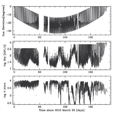
Figure 1: Time-series plots of Sun elevation angle (top panel), sky brightness level (middle panel), and number of stars detected in each image (bottom panel).

3 Photometry

3.1 Frame Selection and Photometry

We carried out initial photometric measurements on the debiased, flattened, sky-subtracted and fringe-corrected images using the same pipeline and procedures described in Wang et al. (2011), which we briefly summarize here. Given the extremely undersampled nature of the images, we performed aperture photometry using DAOPHOT Stetson (1987). We set the aperture radius to 2.5 pixels (equivalent to $39.3\arcsec$) and the sky annulus extended from 4 to 7 pixels (equivalent to $62.8-109.9\arcsec$). The detection threshold was set to $5\sigma$ above the sky background, which typically corresponded to $i\sim 14$ mag.

Figure 1 displays the Sun elevation angle (top panel), sky background in ADU s^-1 (middle panel), and number of stars detected (bottom panel) for each image as a function of time since 2010 March 29. The sky background shows a clear monthly pattern related to the lunar phase. During most of the winter season, the data acquisition system was programmed to stop when the sky level exceeded 14,600 ADU; this limit was raised to 19,400 after 2010 Sep 7. We initially selected frames with Sun elevation angle below $0^{\circ}$ and more than 1,500 stars. These criteria were met by 85.5% (289,343) of all the images acquired during the Antarctic winter. A period of bad weather and ice buildup on the top cover of the instrument during the month of July resulted in the rejection of $\sim$35,000 images (equivalent to 8 days of operations).

The selected images have a median sky level of 32 ADU s^-1, equivalent to a median sky background of $i\!=\!19.8$ mag$/\sq\arcsec$. This value is identical to the value derived by Zou et al. (2010) and similar to our previous determination of 19.6 mag$/\sq\arcsec$ (Wang et al., 2011). Note that all these estimates include contributions from moonlight. The darkest sky background measured during the season (on clear moonless nights) was $i\sim 20.9$ mag$/\sq\arcsec$. The median value of the number of stars detected in an individual frame is 8,600, higher than the corresponding value of 7,500 from the 2008 observations. We attribute this increase to the subtraction of sky background variations described in § 2.2, which enabled the detection of fainter stars at a fixed threshold.

Figure 2: Comparison of the mean instrumental magnitudes of bright stars in common between the 2008 and 2010 CSTAR observations.

We used the initial photometry to register all frames using DAOMATCH and DAOMASTER and created a reference image (hereafter, “master frame”) with $4\times$ finer spatial sampling. We followed the same procedure described in our previous paper, this time based on 2,580 high-quality images obtained during 2010 June 13. We carried out aperture photometry on the master frame using the same parameters listed above and detected approximately 155,000 stars, reaching a depth of $i\sim 20.9$ mag. Additionally, we performed point-spread function photometry that, despite its lower quality due to the undersampled nature of the images, enabled us to estimate the relative magnitudes of stars with overlapping apertures.

3.2 Photometric corrections

We performed all the photometric corrections described in detail in Wang et al. (2011), which included: exposure time normalization, zeropoint correction, sigma rescaling, residual flat fielding, time calibration, masking of satellite trails and saturated regions, spike filtering, and magnitude calibration. We will only discuss the details of magnitude and time calibration since the rest of the procedures were identical to our previous work.

We performed the magnitude calibration by matching the mean instrumental magnitudes of 1,831 stars with $9.3\leq i\leq 12.3$ mag in common between our 2010 and 2008 master frames. Since the mean instrumental magnitudes of each season are referenced to individual images obtained under the best observing conditions (in terms of sky background and number of stars) we would expect them to reflect photometric conditions and therefore have very similar zeropoints. Indeed, we found a zeropoint offset of only $0.018\pm 0.005$ mag as shown in Fig. 2. We transformed the instrumental magnitudes to the Sloan photometric system by applying the offset of $7.45\pm 0.04$ mag previously derived in §3.2 of Wang et al. (2011). That offset was based on the comparison of our photometry with the $i$ synthetic magnitudes derived by Ofek (2008) using the Tycho catalog, which carries an additional systematic uncertainty of 0.02 mag.

Figure 3 shows a time series and a histogram of differential extinction values, based on the photometry procedures described above. We find that extinction due to clouds in the $i$ band at Dome A is less than 0.4 mag during 70% of the dark time, and less that 0.1 mag during 40% of the dark time. These values are similar to those previously derived for the 2008 Antarctic winter season (80% and 50%, respectively, from Wang et al., 2011).

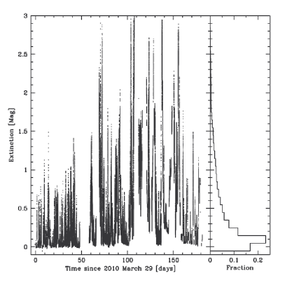
Figure 3: Left panel: time series plots of differential extinction, right panel: distribution of differential extinction.

The computer associated with the CSTAR#3 telescope has a GPS receiver to maintain time synchronization, and this time was to be distributed to computers controlling the other CSTAR telescopes (including the one used for these observations). However, there was a communication problem between the computers throughout the entire observation period, which led to a drift in the time stamp of the FITS images. §4.3 of Zhou et al. (2010a) contains details of the time calibration for the 2008 data; we carried out a similar procedure for the 2010 data as explained below.

We performed the time calibration in three steps. First, we identified two bright stars located very close to R.A.=0h and measured the angle (with respect to the x-axis) of a line extending from the SCP to their positions. We calculated the difference between the measured angle and the one predicted from the time in the FITS headers, and fit a fourth-order polynomial to solve for the time drift. The smallest dispersion was obtained by fitting two different polynomials for the data acquired before and after 2010 June 17. The total clock drift over 6 months amounted to $\sim 190$ seconds as seen in Fig. 4. Next, we used 19 entries in a log (obtained for engineering purposes throughout the season) that listed the time offset between the CSTAR#3 computer and another computer at Dome A which had maintained GPS synchronization. While these data points were not sufficient to solve for the time drift, they served to transform our relative measurements into an absolute reference frame. We obtained an offset of $1337.5\pm 1.6$ s. Lastly, we applied a transformation to the heliocentric reference frame.

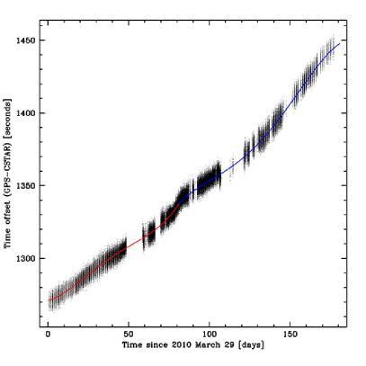
Figure 4: Drift between true local time and computer time, fitted by two fourth-order polynomials.

We later checked the derived time offset by performing a cross-correlation of the light curves of 33 bright, high-amplitude, periodic variables (such as eclipsing binaries and RR Lyraes) that we had previously detected in Wang et al. (2011). We used the latest implementation of the Phase Dispersion Minimization algorithm (Stellingwerf, 1978, 2011), which can robustly handle large gaps in the time series and combines all light curve “segments” to determine a common period. Using this approach, we found a consistent (but less precise) offset of $1270\pm 245$ s.

4 Variable Stars in the CSTAR field

While the primary goal of CSTAR observations is to characterize the observing conditions at Dome A, the rapid cadence of image acquisition and the long duration of the winter night make this a relatively unique data set for studying variable stars and searching for extrasolar planets via the transit method. We used several complementary techniques (described below) to identify variables among the selected stars, since no single approach is sensitive to all types of stellar variability. Some of the methods we used are only sensitive to periodic variability. Most of the algorithms we used are available as part of the VARTOOLS light curve analysis program of Hartman et al. (2008).

Having already characterized the observing conditions at the site based on all the “dark time” data, we restricted our variable-star analysis to the images obtained under the best observing conditions, which we defined as a sky background below 100 ADU s^-1 and an extinction $\leq 0.5$ mag. These criteria were met by $169{,}500$ frames (the “science-quality” sample), corresponding to about 60.9% of the previously selected set of images. Among the rejected images, 3.7% failed to provide a reliable coordinate transformation with respect to the reference frame.

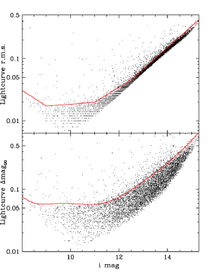
Figure 5: r.m.s. (top) and 90%-ile magnitude range (bottom) of the lightcurves of $9{,}125$ selected stars with sufficient synoptic coverage (see text for details).

We initially selected the brightest $20{,}000$ stars in the master frame (corresponding to a depth of $i\sim 15.3$ mag) for time-series aperture photometry. Once the measurements were carried out, we restricted our analysis to $9{,}125$ objects with valid measurements in at least 20% of the individual science-quality frames (or in 20% of all possible 3,000s time segments) in order to ensure sufficient synoptic coverage. This restriction implies a maximum declination limit of $-87^{\circ}13\arcmin$ for objects in the sample, which we will later use when comparing our variable star statistics with previous studies.

We complemented the search for variables with information obtained from the PSF photometry previously carried out on the master frame, which had a $4\times$ finer pixel scale and represented a 24-hour average stellar flux. For each object of interest, we calculated the fraction of contaminating flux contributed all other stars located closer than a certain distance: the aperture radius ($39.3\arcsec$), the inner edge of the sky annulus ($62.8\arcsec$), and the outer edge of the sky annulus ($109.9\arcsec$). We refer to these three fluxes hereafter as “close”, “medium” and “far” respectively.

Figure 6: Variability statistic $J$ (Stetson, 1996) for $9{,}125$ selected stars with sufficient synoptic coverage (see text for details).

4.1 Search for variability

The first phase of our search for variable stars was aimed at identifying objects with statistically significant variations in magnitude that did not necessarily display a periodic behavior during our observations – including objects such as Miras, other very long-period variables and irregular variables. We used a combination of three metrics to separate constant from variable stars, as detailed below.

We calculated the r.m.s. and the magnitude range spanned by 90% of data points (hereafter, $\Delta i_{90}$) of the light curves of all stars. We determined upper $2\sigma$ envelopes for both quantities as a function of magnitude, shown with red lines in Fig. 5. Stars lying above both envelopes were flagged as possible variables for further analysis. The upturn in both envelopes for $i<9$ mag is probably due to a combination of factors, including the onset of non-linearity in the detector and the dearth of truly constant stars in this magnitude range within our field. The Besançon model of the Galaxy (Robin et al., 2003) predicts that post-main sequence stars (which are very likely to exhibit variability, see Henry et al., 2000) will outnumber main-sequence objects by a ratio of 7 to 1 at this magnitude.

The lowest light curve r.m.s. values (7 mmag) are found at $i\sim 10$ mag, reaching within a factor of 5 of the expected scatter due to scintillation (Young, 1967) for our telescope at Dome A. Given the large number of individual measurements in our photometry, bright ($i<13.5$ mag) stars lying below both envelopes have statistical uncertainties in their mean magnitudes below $2\times 10^{-4}$ mag. As discussed in §3.2 and in Wang et al. (2011), the overall uncertainty of the photometry is dominated by the statistical ($\pm 0.04$ mag) and systematic ($\pm 0.02$ mag) uncertainties of the calibration procedure.

Next, we computed the Welch-Stetson variability index $J$ (§2 of Stetson, 1996), including the usual rescaling of the reported DAOPHOT magnitude errors (Udalski et al., 1994; Kaluzny et al., 1998). The result of this analysis is shown in Fig. 6; as expected for the $J$ statistic, there is a gaussian distribution of values with a mean value close to zero (corresponding to stars with no significant variability), and a one-sided tail (towards positive values) of candidate variable stars. We determined a mean value of $J=0.049\pm 0.038$ by fitting a Gaussian function to all objects with $|J|<0.3$, and flagged stars with $J\geq 0.164$ (equivalent to a $+3\sigma$ selection) for further inspection.

We combined the r.m.s., $\Delta i_{90}$ and $J$ criteria listed above to select 44 variable stars. In addition to passing all 3 variability criteria, the selected objects were also restricted to have contaminating fluxes from nearby companions in the “medium” and “far” apertures below 11.5% and 23% of the total flux, respectively. These limits may have resulted in the rejection of some bona fide aperiodic variables or transient events, but they serve to eliminate false positives from our sample.

4.2 Search for periodic variability

The $J$ statistic was designed to be sensitive to statistically significant photometric variability between neighboring data points, and is well suited to detect continuously-varying objects such as pulsating stars (Miras, Cepheids, RR Lyrae, $\delta$ Scuti, etc.) or contact binaries. It is not particularly sensitive to detached eclipsing binaries (where the variation is restricted to a very small fraction of the phase) or to objects where the variation only becomes statistically significant after phasing many cycles (such as transiting exoplanets or very low amplitude pulsators). Similarly, the other two metrics used in the first phase of the search for variables (light curve r.m.s. and $\Delta i_{90}$) lack sensitivity to small-scale periodic variations. Therefore, we searched for periodic variability among the stars that had failed one or more of the previous selection criteria using two of the techniques described in detail in Wang et al. (2011): the Lomb-Scargle method (Lomb, 1976; Scargle, 1982, hereafter LS) and the “box fitting algorithm” of Kovács et al. (2002, hereafter BLS).

Given the design of the CSTAR system, stars describe daily circular tracks through the CCD. This can lead to spurious detections of periodicity due to small residual flat-field variations. Fortunately, these false positives are easily identified and discarded because the variations occur at frequencies close (0.5-3%) to 1 cycle per sidereal day and their (sub-)harmonics. We considered an object to have significant periodic variability if the period determined by VARTOOLS (based on either the LS or the BLS technique) had a SNR$>30$ and lied outside of the excluded frequencies. We imposed a minimal restriction on contaminating flux for this search, removing 2% of objects where the contaminating flux from other stars in the “close” aperture exceeded 40% of the total. The search for periodic variables can tolerate substantially larger contamination from neighbors for several reasons: very close neighbors (within the instrumental PSF or the measurement aperture) can only decrease the amplitude of the variation but cannot result in a false positive, and future observations can be used to identify which of the confused stars is the actual variable; stars outside the measurement aperture but within the outer sky annulus may produce noisier measurements but the long span of our observations still yields high-quality binned light curves that satisfy the requirement on the SNR of the period determination; any companions that somehow induce a spurious periodic variation will do so at frequencies of 1 cycle/day or one of its harmonics and those have already been removed from consideration.

We detected an additional 136 variables using the LS technique and a further 8 variables using the BLS technique. These algorithms were also applied to the variables previously selected in §4.1 and 16 of those objects were found to exhibit a significant periodicity. The initial periods were refined using the Period04 program (Lenz & Breger, 2005) and the Phase Dispersion Minimization algorithm (Stellingwerf, 1978, 2011).

Approximately two thirds of the periodic variables exhibit a highly regular variation both in terms of period and amplitude (e.g., eclipsing binaries, normal RR Lyraes), a few have a long-term modulation in amplitude (e.g., Blazhko RR Lyraes), and about one third show variations at multiple frequencies. In the latter two cases, we based our analysis in the most significant period.

4.3 Properties of variable stars

Table 8 lists the properties of all detected variables. Column 1 has the 2010 CSTAR ID (a letter n is added at the beginning to avoid confusion with 2008 CSTAR IDs from our previous work); column 2 lists the 2008 CSTAR ID from (Wang et al., 2011), if applicable; column 3 presents the ID from the Guide Star Catalog, version 2.3.2 (GSC2.3), when available; columns 4 and 5 give the right ascension and declination; column 6 contains the mean $i$-band magnitude; column 7 lists the 90% range of the $i$-band light curve; column 8 has the $J$ value; column 9 lists the most significant period (when applicable); column 10 specifies the technique used to find the period; column 11 gives the first time of minimum light contained in our observations (listed only for the periodic variables); column 12 contains a tentative classification of the variable type, when possible; column 13 has additional information, including previous identification of the variables by the All-Sky Automated Survey (Pojmanski, 2005, ASAS,) or inclusion in the General Catalogue of Variable Stars (GCVS, Samus et al., 2009). Representative light curves of periodic variables are shown in Fig. 7, while two-season light curves of selected long-term variables are plotted in Fig. 8. Detailed finding charts including light curve plots for all variables are available through the Chinese Virtual Observatory. All light curve data is also available through this site.

We detected a total of $188$ variables in the 2010 CSTAR data, consisting of $67$ new objects and $121$ stars in common with Wang et al. (2011). We did not recover 36 objects classified as variables in our previous paper for the following reasons: 10 did not have enough data points, 7 were blended, and 19 did not meet the selection criteria adopted in this paper. The new variables detected in this study relative to our previous work were made possible by the deeper magnitude limit and slightly larger field of view ($\delta<-87^{\circ}13\arcmin$) of the 2010 observations, which were respectively due to better sky subtraction and improved alignment of the center of the field with the SCP.

Thanks to the greater depth and synoptic   coverage   of   our   observations,   we obtained   a   $\sim 4\times$   increase   in   the number   of   variables   with   $\delta<-87^{\circ}13\arcmin$  relative  to

Figure 7: Phased light curves of six newly detected periodic variable stars. The periods and 2010 CSTAR IDs are given above each panel. Top row: transiting exoplanet candidate and detached eclipsing binary; middle row: RR Lyrae and $\delta$ Scuti; bottom row: multi-periodic variables phased at the most significant period.

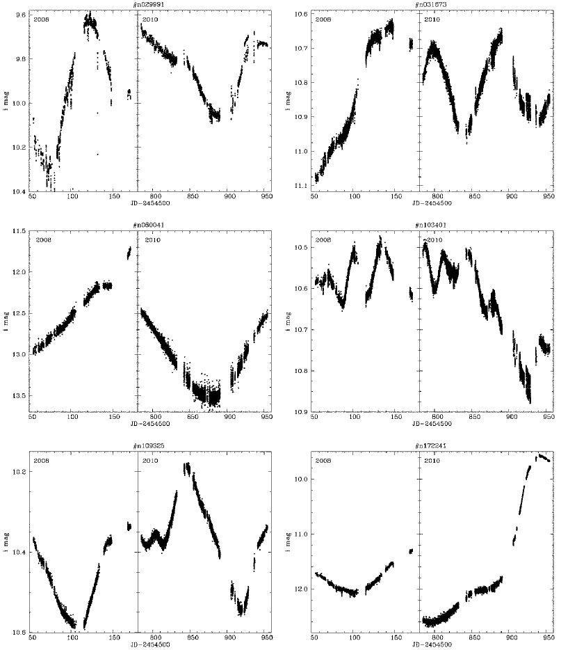
Figure 8: Two-year light curves (left: 2008; right: 2010) for variables with long-term trends.

lllllrrrrlrll 0pt Variable stars ID R.A. Dec. $i$ $\Delta i_{90}$ $J$ Period $T_{0}^{3}$ Class⁴ Note⁵
2010 2008 GSC (J2000.0)¹ (mag) (d) Src² (d) n010320 & $\dots$ S742000016 12:04:48.75 $-$87:23:06.0 8.79 0.18 9.68 $\dots$ $\dots$ $\dots$ IR A
n012443 001707 S74D000321 12:32:42.91 $-$87:26:22.9 11.10 0.55 9.95 0.338544 LS 785.6824 EC A
n012506 $\dots$ S3Y9000067 11:44:32.67 $-$87:27:35.9 10.89 0.12 2.07 31.447988 LS $\dots$ MP
n015318 003125 S3YM000469 10:43:46.63 $-$87:25:10.1 9.69 0.09 3.32 3.602742 LS $\dots$ MP
n015705 $\dots$ S3YM000358 10:04:32.92 $-$87:13:44.7 10.97 0.08 0.65 19.081678 LS $\dots$ MP
n016257 003697 S742000061 12:08:11.93 $-$87:35:39.9 11.56 0.08 0.75 26.567900 LS $\dots$ MP
n016505 003850 S742000043 12:34:25.12 $-$87:34:37.7 10.14 0.06 1.59 17.251594 LS $\dots$ MP A
n017573 004463 S3YM000518 10:40:16.05 $-$87:29:29.8 11.16 0.06 0.58 0.869262 LS 785.7941 ED
n017781 $\dots$ S74D000351 13:21:24.66 $-$87:29:48.4 12.41 0.10 0.25 4.822329 LS $\dots$ MP
n020508 $\dots$ S74D000440 13:01:58.40 $-$87:39:56.3 9.01 0.16 3.11 5.798380 LS 786.5008 ED
n023757 $\dots$ S3YM000018 09:51:32.15 $-$87:28:32.7 13.24 0.18 0.20 0.240900 LS 785.4140 PR
n024696 009171 S3YM000662 10:12:54.85 $-$87:38:22.9 14.10 0.77 1.29 0.591726 LS 785.4091 RL A
n025073 $\dots$ S3YN000420 09:29:27.99 $-$87:21:39.6 9.01 0.32 18.03 $\dots$ $\dots$ $\dots$ IR A
n025734 009952 S742000182 12:43:30.67 $-$87:53:30.9 11.30 0.20 2.89 23.819339 LS $\dots$ MP A
n027942 011616 S3Y9000240 10:56:28.86 $-$87:55:21.0 11.97 0.08 0.55 27.282715 LS $\dots$ MP
n028073 011709 S742000246 12:41:44.27 $-$87:58:28.5 11.37 0.07 0.77 2.951167 LS 787.1734 PR
n028235 011796 S742000286 12:21:35.82 $-$88:00:14.5 12.20 0.26 0.90 1.892910 LS 786.9435 ES
n029044 $\dots$ S742000186 13:28:28.82 $-$87:53:09.2 9.52 0.04 1.86 11.564653 LS $\dots$ MP
n029991 013255 S74F000377 14:54:21.37 $-$87:21:05.0 9.87 0.34 6.41 $\dots$ $\dots$ $\dots$ IR A
n030008 013140 S3Y9000236 10:25:53.99 $-$87:53:40.8 9.83 0.07 1.40 20.978237 LS $\dots$ MP
n031343 014111 S74F000634 14:29:01.63 $-$87:38:16.2 13.74 0.42 0.67 0.174082 LS 785.3263 DS
n031673 014368 S3YM000753 10:03:10.79 $-$87:51:06.2 10.81 0.25 5.38 95.147196 LS $\dots$ MP
n031801 014495 S3Y9000339 10:49:00.65 $-$88:02:17.2 12.30 0.12 0.65 19.218473 LS $\dots$ MP
n034888 016836 S742030458 12:49:16.22 $-$88:11:17.6 13.74 0.30 0.47 0.176214 LS 785.2034 DS
n035474 $\dots$ S74F007170 15:09:55.59 $-$87:25:01.9 9.09 0.08 2.89 $\dots$ $\dots$ $\dots$ IR
n037305 018708 S3YN000609 09:02:20.82 $-$87:37:41.0 12.38 0.09 0.25 1.627880 LS 785.2541 ES
n039537 020436 S3YN000517 08:40:33.28 $-$87:28:38.6 12.60 0.23 0.76 61.305131 LS $\dots$ MP
n039664 020526 S742000504 13:23:49.26 $-$88:16:04.3 12.46 0.42 1.53 2.510726 LS 786.9545 ES A
n040035 $\dots$ S3Y9000616 11:52:51.12 $-$88:23:28.9 9.21 0.06 1.73 17.086312 LS $\dots$ MP
n042221 022489 S3Y9000527 10:01:21.80 $-$88:13:30.8 11.89 0.22 2.51 0.652314 LS 785.7043 EC A
n043406 $\dots$ S3YN000632 08:39:40.85 $-$87:39:02.3 12.21 0.10 0.26 7.165431 BLS 787.9603 ED
n043566 023614 S742000638 12:09:34.38 $-$88:29:59.0 11.49 0.05 0.32 17.256627 LS $\dots$ MP
n044666 $\dots$ S3Y9000612 10:32:32.73 $-$88:25:02.6 13.73 0.14 0.09 3.535402 BLS 788.5108 ED
n045656 $\dots$ S742000672 14:20:52.04 $-$88:14:33.4 12.65 0.08 0.25 0.400924 LS 785.2228 EC
n045983 025440 S742000656 12:12:56.28 $-$88:34:11.6 10.77 0.03 0.37 9.972472 LS $\dots$ MP
n046511 025846 S742000671 14:25:39.12 $-$88:14:54.1 13.77 0.14 0.07 9.618211 LS 788.7800 PR
n047552 026640 S3YB000429 11:17:00.40 $-$88:35:36.4 9.37 0.38 10.24 $\dots$ $\dots$ $\dots$ LT A
n047660 026730 S3YB000202 09:58:36.02 $-$88:23:59.9 12.89 0.11 0.13 2.066699 LS 786.2584 ED
n049496 028221 S3YB000436 11:04:06.48 $-$88:38:02.5 13.55 0.25 0.38 4.815779 LS 788.6982 PR
n050944 029379 S74E000029 15:57:05.68 $-$87:30:05.4 11.93 0.15 0.99 1.553117 LS $\dots$ MP A
n052190 030353 S3YA000615 08:39:40.45 $-$88:03:19.4 12.87 0.09 0.15 1.048425 LS 785.9799 PR
n052325 $\dots$ S74E000072 15:44:44.17 $-$87:46:35.4 8.35 0.09 5.76 $\dots$ $\dots$ $\dots$ IR
n054284 032007 S3YB000225 09:29:39.14 $-$88:30:06.4 11.78 0.12 0.98 0.621863 LS 785.5950 RL A,G
n054942 032544 S3Y8000312 11:48:09.42 $-$88:49:52.6 10.39 0.05 1.27 25.795462 LS $\dots$ MP
n055150 $\dots$ S3YB000458 10:04:40.34 $-$88:40:25.5 9.06 0.04 1.41 0.092508 LS 785.2723 PR
n057617 034669 S743000094 13:50:03.38 $-$88:46:13.2 10.08 0.06 1.40 15.167192 LS $\dots$ MP
n057725 034724 S3YB000482 10:01:18.94 $-$88:44:36.8 10.08 0.10 2.34 43.205800 LS $\dots$ MP A
n057789 $\dots$ S3Y8000318 11:19:13.27 $-$88:53:40.8 12.74 0.10 0.19 1.862438 LS $\dots$ MP
n058002 034997 S743000311 14:29:04.38 $-$88:38:43.7 12.13 0.61 5.88 0.646577 LS 785.6753 RL A
n058442 $\dots$ S3YB000199 08:53:45.85 $-$88:26:33.0 12.41 0.07 0.21 0.258295 LS 785.2335 PR
n058656 035468 S3YA000613 08:08:46.28 $-$88:00:02.0 13.86 0.17 0.09 0.822773 BLS 786.0050 ED
n059543 036162 S3YB000243 09:03:59.29 $-$88:33:07.6 11.40 0.20 1.18 0.873857 LS 785.2020 ES A
n060041 036526 S743000153 15:35:01.14 $-$88:16:11.9 13.16 0.95 4.98 $\dots$ $\dots$ $\dots$ LT
n060566 036939 S743000200 15:25:11.74 $-$88:23:14.9 12.82 0.05 0.05 7.376734 LS 785.7479 PR
n060667 037016 S743000186 15:28:41.36 $-$88:21:44.0 13.63 0.15 0.10 0.157962 LS 785.3571 PR
n060789 $\dots$ S741000025 15:59:17.54 $-$88:00:42.5 14.23 0.26 0.03 6.853790 LS 789.0467 ED
n062144 038255 S743000115 13:53:18.49 $-$88:54:14.6 12.87 0.47 2.17 0.266903 LS 785.2292 EC A
n062519 038580 S3Y8000346 10:50:11.96 $-$88:59:54.1 11.78 0.05 0.21 5.745575 LS 787.1325 PR
n062640 038663 S3YB000253 08:46:12.64 $-$88:33:42.9 12.00 0.44 5.22 0.267127 LS 785.2565 EC A
n062696 $\dots$ S741000340 16:07:56.96 $-$87:59:09.7 11.98 0.08 0.31 1.185502 LS 785.2992 PR
n062884 $\dots$ S740000057 12:30:49.10 $-$89:02:45.7 11.94 0.03 0.06 25.125450 LS 787.7145 PR
n063743 039541 S740000060 12:36:24.67 $-$89:04:02.7 10.97 0.04 0.46 25.161758 LS $\dots$ MP
n064731 040351 S3YA000660 08:02:26.52 $-$88:14:26.1 13.34 0.11 0.13 0.285606 LS 785.4430 PR
n065137 $\dots$ S74E000575 16:31:36.82 $-$87:40:07.7 12.11 0.09 0.27 5.388951 LS 790.4191 ED
n066680 $\dots$ S3YL000291 07:14:42.32 $-$87:22:25.0 11.37 0.07 0.49 $\dots$ $\dots$ $\dots$ IR
n066932 $\dots$ S743000330 15:21:39.34 $-$88:41:59.3 13.00 0.06 0.07 20.753202 LS 785.2020 PR
n068660 043618 S3YB009826 08:40:28.89 $-$88:47:00.4 13.72 0.33 0.26 13.024607 LS 794.0587 ES
n069025 043885 S3YB000275 08:17:16.96 $-$88:37:29.5 14.00 0.17 0.09 9.386448 LS 785.9529 PR
n070113 044751 S740000101 13:01:29.04 $-$89:13:47.0 13.21 0.11 0.14 6.422671 LS 787.0902 PR
n073013 047176 S3YA000181 07:12:14.54 $-$87:51:19.7 12.81 0.15 0.42 2.643748 LS 786.7776 PR
n076289 $\dots$ S3YA000320 07:07:52.74 $-$88:02:11.4 12.94 0.10 0.13 0.789882 LS 785.4483 PR
n076976 050375 S3YB013754 07:39:17.11 $-$88:40:41.7 13.46 0.10 0.06 1.441150 LS 785.6660 PR
n077512 050773 S74E000469 17:10:42.44 $-$87:30:09.3 10.52 0.06 1.12 3.292027 LS $\dots$ MP
n078642 $\dots$ S3Y8000239 08:51:51.07 $-$89:15:21.3 12.27 0.05 0.09 3.481819 LS 785.5641 PR
n080090 052891 S741000155 17:13:18.69 $-$87:42:28.6 9.44 0.17 8.41 59.365516 LS $\dots$ MP A
n080626 $\dots$ S743000493 16:37:09.46 $-$88:43:24.2 11.29 0.04 0.23 35.753464 LS $\dots$ MP
n080649 $\dots$ S3YA000502 07:01:38.41 $-$88:17:02.9 9.60 0.05 1.52 23.466222 LS $\dots$ MP
n080770 053446 S3Y8000220 08:05:03.24 $-$89:07:54.3 12.95 0.13 0.20 1.071988 LS 786.1217 PR
n080929 053570 S743000460 16:44:10.40 $-$88:38:19.9 11.02 0.03 0.26 19.967817 LS $\dots$ MP
n081202 053783 S3Y8000272 09:44:14.75 $-$89:28:17.6 10.48 0.02 0.18 16.047868 LS $\dots$ MP
n083000 $\dots$ S3Y8007194 09:23:04.69 $-$89:29:38.8 13.77 0.23 0.25 0.124657 LS 785.2675 PR
n083359 055495 S3Y8000078 07:43:54.49 $-$89:07:37.3 12.52 0.39 1.45 0.797910 LS 785.8882 EC A
n084427 055854 S3Y8000109 07:54:37.65 $-$89:15:40.9 9.75 0.08 1.67 $\dots$ $\dots$ $\dots$ IR
n085632 057344 S741000539 17:13:42.52 $-$88:24:52.5 11.09 0.09 1.60 20.106163 LS $\dots$ MP
n086263 057775 S3YA000492 06:40:47.15 $-$88:15:21.3 11.73 0.39 4.71 0.438659 LS 785.4511 EC A
n088489 $\dots$ S3YA016263 06:31:32.66 $-$88:11:38.1 12.81 0.09 0.13 0.240723 LS 785.4360 PR
n088653 059811 S3YA000336 06:28:42.76 $-$88:02:41.7 12.35 0.12 0.23 7.254001 LS 787.3637 ED
n090586 061353 S740000342 17:15:45.51 $-$89:00:42.8 10.78 0.02 0.18 0.022641 LS 785.2130 PR
n090919 061658 S741000489 17:36:45.98 $-$88:14:10.5 11.31 0.03 0.24 0.076166 LS 785.2522 PR
n091083 061740 S740000322 17:23:25.05 $-$88:53:37.3 9.99 0.07 2.20 34.479083 LS $\dots$ MP
n091084 061783 S740000308 17:25:37.17 $-$88:49:50.3 13.83 0.35 0.35 0.188993 LS 785.3176 DS
n092211 062683 S3Y8000165 07:46:18.25 $-$89:40:00.7 10.27 0.04 0.75 15.857866 LS $\dots$ MP
n094368 064380 S3YA000248 06:10:28.12 $-$87:53:32.9 14.20 0.24 0.03 2.307363 LS 785.2020 PR
n095083 064944 S741000460 17:51:13.16 $-$88:09:48.8 10.65 0.05 0.96 30.763139 LS $\dots$ MP
n095145 065072 S740000301 17:47:26.35 $-$88:46:07.9 11.87 0.05 0.18 0.620534 LS 785.6897 PR
n096554 066196 S740000469 17:05:16.14 $-$89:51:43.8 9.67 0.04 1.06 26.623757 LS $\dots$ MP
n097049 $\dots$ S740012990 17:55:19.53 $-$89:07:43.2 14.97 0.56 0.14 0.348088 LS 785.2424 PR
n097333 066775 S741000378 17:59:00.73 $-$88:01:32.9 11.76 0.18 1.86 38.853950 LS $\dots$ MP
n099251 068276 SA9S000144 18:22:33.29 $-$89:36:22.9 11.39 0.03 0.20 2.835357 LS 786.8351 PR
n099286 068308 S0SG000353 05:50:34.20 $-$89:06:46.2 12.94 0.08 0.10 0.798947 LS 785.3570 PR
n100083 068908 SA9U000383 18:08:15.09 $-$88:18:02.9 10.83 0.03 0.33 2.842765 LS $\dots$ MP
n101873 $\dots$ S0SH000511 05:43:48.57 $-$88:32:56.9 12.75 0.12 0.22 0.646457 LS 785.3882 PR
n102304 070680 SA9S000413 22:05:02.55 $-$89:52:06.7 13.05 0.21 0.56 1.988474 LS 787.1308 ES
n102641 070941 S0SH000215 05:47:08.05 $-$87:51:00.2 10.23 0.05 1.21 0.606546 LS 785.4046 GD
n103401 071571 S0SH000333 05:43:19.93 $-$88:04:04.3 10.65 0.32 6.76 $\dots$ $\dots$ $\dots$ LT A
n104524 072350 SA9V000050 18:30:57.87 $-$88:43:17.5 9.86 0.04 0.57 9.925551 BLS 788.2407 TR
n104943 072730 SA9U000438 18:29:03.93 $-$88:32:31.9 13.32 0.51 1.85 0.573044 LS 785.7601 RL A
n105244 $\dots$ S0SG000150 00:20:19.58 $-$89:48:38.0 9.43 0.04 1.22 10.923423 LS $\dots$ MP
n108372 $\dots$ SA9S000233 20:34:48.30 $-$89:34:03.2 12.81 0.07 0.12 2.371811 LS 785.4818 PR
n109325 076135 SA9S000115 19:53:21.15 $-$89:22:46.5 10.37 0.33 8.00 $\dots$ $\dots$ $\dots$ IR
n110028 076723 SA9V000063 19:00:22.60 $-$88:47:53.7 10.88 0.21 4.41 $\dots$ $\dots$ $\dots$ IR
n110665 077190 S0SH000448 05:15:49.62 $-$88:17:51.5 10.21 0.04 0.92 11.462763 LS $\dots$ MP
n111158 077508 SA9S000404 22:53:06.46 $-$89:38:40.9 14.07 0.36 0.09 0.133318 LS 785.3185 PR
n111246 077594 SA9V000067 19:08:12.87 $-$88:49:18.5 10.06 0.02 0.48 1.679604 LS 785.5144 PR
n112440 078549 S0SH000321 05:15:49.03 $-$88:04:23.5 13.12 0.16 0.42 5.389812 LS 787.9077 PR
n112694 078773 SA9V000073 19:17:53.08 $-$88:51:11.2 11.81 0.09 0.68 0.372068 LS 785.2474 EC
n113158 $\dots$ SA9S000043 19:33:21.70 $-$89:00:22.9 8.67 0.17 2.29 $\dots$ $\dots$ $\dots$ IR A
n113486 079397 SA9S000068 19:48:57.10 $-$89:07:14.3 10.86 0.02 0.21 4.842585 LS 788.1947 PR
n114115 $\dots$ S0SG000229 03:01:17.31 $-$89:24:30.2 12.38 0.05 0.08 5.767268 BLS 785.6845 TR
n115348 080934 SA9U000331 18:58:35.51 $-$88:12:55.2 11.72 0.24 2.83 62.185489 LS $\dots$ MP
n116034 $\dots$ S0SH000139 05:12:14.90 $-$87:44:42.1 8.43 0.13 8.84 $\dots$ $\dots$ $\dots$ IR A
n116344 081723 SA9U000071 18:48:23.75 $-$87:43:16.4 11.49 0.07 0.67 0.841671 LS 785.5572 GD
n116380 081749 $\dots$ 19:11:53.61 $-$88:27:14.9 10.31 0.03 0.54 88.385466 LS $\dots$ MP
n116491 081845 SA9V000074 19:38:27.80 $-$88:50:55.9 12.90 0.10 0.09 6.759592 LS 785.3202 ED
n116918 082180 S0SG000129 00:29:58.19 $-$89:30:20.3 11.24 0.02 0.15 0.152825 LS 785.3478 DS
n117549 $\dots$ S0SG000213 02:55:59.73 $-$89:17:48.2 12.48 0.06 0.11 0.721620 LS 785.4964 PR
n117763 $\dots$ SA9U000396 19:13:28.77 $-$88:21:56.0 12.84 0.12 0.27 0.151852 LS 785.2020 DS
n118098 083110 S0SG000226 02:11:02.80 $-$89:22:50.3 10.27 0.03 0.43 6.623027 LS $\dots$ MP
n118528 $\dots$ SA9S000384 23:35:11.99 $-$89:27:51.8 14.78 1.23 0.86 0.465790 LS 785.3995 RL G
n118992 $\dots$ SA9S000200 21:24:11.87 $-$89:17:56.5 14.69 0.52 0.15 0.233625 LS 785.2898 DS
n119729 084344 SA9S000371 23:01:30.03 $-$89:25:01.5 13.96 0.18 0.07 2.927708 BLS 786.0597 PR
n121493 085719 S0SG000178 03:08:19.12 $-$89:06:32.2 12.20 0.06 0.18 17.205471 LS $\dots$ MP
n122451 086480 S0SJ000306 03:44:10.88 $-$88:52:09.5 11.19 0.03 0.22 21.496218 LS $\dots$ MP
n122836 $\dots$ SAA5000323 19:02:33.97 $-$87:35:30.2 8.86 0.07 2.42 $\dots$ $\dots$ $\dots$ IR
n123187 087084 SA9S000168 20:57:31.47 $-$89:03:50.3 12.36 0.33 0.76 1.857642 LS 786.7030 ED
n123522 $\dots$ SA9U000336 19:27:57.26 $-$88:13:26.2 8.80 0.32 17.60 $\dots$ $\dots$ $\dots$ IR A
n123706 087501 S0SG000092 01:23:01.27 $-$89:17:09.4 13.60 0.20 0.12 0.193489 LS 785.3819 DS
n123782 087548 S0SH000485 04:20:11.85 $-$88:25:03.5 12.63 0.12 0.61 0.197741 LS 785.2566 DS
n124517 088142 S0SG000093 00:52:40.76 $-$89:17:32.4 13.84 0.38 0.41 0.292944 LS 785.3965 EC
n126026 089391 SA9U000387 19:43:40.77 $-$88:19:20.7 13.49 0.08 0.04 0.136874 LS 785.3534 PR
n128266 $\dots$ S0SJ000248 03:37:18.58 $-$88:38:51.4 9.47 0.04 0.95 7.957924 LS $\dots$ MP
n130449 $\dots$ S0SG000064 00:24:32.27 $-$89:08:48.5 12.69 0.08 0.16 4.314518 LS 789.0505 PR
n131494 093873 SA9S000300 22:17:44.44 $-$89:01:38.1 9.45 0.10 4.05 $\dots$ $\dots$ $\dots$ IR
n132580 094793 S0SU000407 04:36:31.02 $-$87:28:03.3 10.97 0.09 1.50 0.617076 LS 785.5155 PR
n132830 $\dots$ S0SH031178 04:00:54.92 $-$88:09:59.6 14.40 0.25 -0.00 0.159051 BLS 785.2264 PR
n133214 $\dots$ S0SJ000325 02:03:09.66 $-$88:55:31.4 12.04 0.04 0.13 0.444790 LS 785.3150 PR
n134610 096404 SAA5000420 19:43:05.07 $-$87:46:52.4 14.13 0.81 1.38 0.581666 LS 785.3416 RL A
n134728 $\dots$ S0SJ014770 03:14:01.11 $-$88:32:53.1 14.42 0.39 0.07 1.209346 LS 785.8792 ED
n135670 097230 SA9U000295 20:02:18.84 $-$88:02:50.0 12.08 0.10 0.21 9.548319 LS 789.9965 ED
n136750 098092 S0SH000022 03:54:41.13 $-$88:02:50.6 11.61 0.16 2.12 74.090207 LS $\dots$ MP A
n137559 098719 SAA5000417 19:50:26.13 $-$87:44:50.7 12.86 0.25 1.07 0.416436 LS 785.3327 EC
n138555 099529 S0SG000018 00:31:15.83 $-$88:55:17.9 10.80 0.03 0.27 9.422044 LS $\dots$ MP
n140799 $\dots$ S0SJ016907 02:29:57.18 $-$88:34:35.3 14.32 0.22 -0.01 2.852904 LS 787.3254 PR
n142023 $\dots$ S0SH031869 03:31:30.30 $-$88:04:24.4 14.45 0.34 0.07 0.722102 LS 785.7695 ES
n142074 $\dots$ SA9V000177 21:19:45.21 $-$88:28:17.7 13.39 0.16 0.21 43.638939 LS $\dots$ MP
n142981 $\dots$ S0SJ000161 02:41:54.21 $-$88:26:02.9 10.98 0.04 0.47 11.204593 LS $\dots$ MP
n145245 $\dots$ S0SJ000052 00:56:07.00 $-$88:42:17.9 11.36 0.04 0.25 7.994425 LS $\dots$ MP
n145960 $\dots$ S0SJ000031 01:51:34.69 $-$88:33:26.9 12.01 0.06 0.27 10.882430 LS $\dots$ MP
n148233 107478 SAA5000503 20:28:30.07 $-$87:46:16.5 11.81 0.17 0.89 2.192580 LS 786.0746 ED
n148619 $\dots$ SA9V011956 22:28:21.41 $-$88:31:41.0 14.34 0.22 0.01 3.817432 LS 788.6046 PR
n149414 $\dots$ S0SJ000002 03:00:33.53 $-$88:02:59.2 10.13 0.86 29.50 $\dots$ $\dots$ $\dots$ LT A,G
n150808 $\dots$ SA9T000439 23:03:39.20 $-$88:32:14.0 10.34 0.10 2.92 $\dots$ $\dots$ $\dots$ IR A
n152437 110801 S0SI000269 02:42:27.87 $-$88:04:22.5 9.46 0.13 4.84 44.303305 LS $\dots$ MP A
n153006 111298 S0SI000438 02:12:56.05 $-$88:13:52.5 10.03 0.04 1.11 12.116866 LS $\dots$ MP
n156482 $\dots$ SA9T000422 23:57:27.17 $-$88:24:54.5 12.44 0.06 0.11 6.198528 LS 788.5551 ED
n157627 $\dots$ S0SV000431 03:10:59.88 $-$87:35:38.1 10.61 0.08 1.16 $\dots$ $\dots$ $\dots$ IR
n159243 $\dots$ S0SI000372 00:00:50.89 $-$88:19:41.9 9.44 0.04 1.12 0.114436 LS 785.2310 PR
n160137 117654 S0ST000503 02:18:11.67 $-$87:56:11.2 10.57 0.09 1.68 22.012562 LS $\dots$ MP
n161425 118705 S0SI033411 00:53:26.68 $-$88:12:41.4 13.40 0.09 0.06 3.535402 BLS 786.7269 TR
n162294 119488 S0SI000329 00:08:43.43 $-$88:13:48.4 10.07 0.11 3.59 $\dots$ $\dots$ $\dots$ IR
n163148 120188 S0SI000289 00:55:45.92 $-$88:09:11.0 11.18 0.06 0.53 10.923423 LS $\dots$ MP
n163888 $\dots$ SA9T000268 22:46:01.56 $-$88:04:59.2 13.88 0.24 0.09 7.752665 LS 787.3176 ED
n164527 121369 SA9T000310 23:15:35.46 $-$88:07:33.8 10.78 0.05 0.75 24.945468 LS $\dots$ MP
n167071 $\dots$ SAA6000049 21:52:26.36 $-$87:44:20.6 10.59 0.05 0.82 10.560170 LS $\dots$ MP
n167300 $\dots$ SAA7000327 21:12:08.31 $-$87:24:25.1 9.17 0.08 2.21 0.166200 LS $\dots$ MP
n167522 123934 SA9T000282 23:52:30.36 $-$88:03:49.5 13.94 0.14 0.04 0.122034 LS 785.2471 PR
n167944 $\dots$ S0SV012740 02:52:25.60 $-$87:20:21.5 13.66 1.03 5.74 $\dots$ $\dots$ $\dots$ LT
n168446 124666 SAA6000034 21:47:16.29 $-$87:39:06.6 12.84 0.62 3.88 0.458059 LS 785.5620 RL A
n171256 $\dots$ SA9T000182 23:16:45.97 $-$87:54:16.6 11.95 0.07 0.29 8.754028 LS $\dots$ MP
n172241 127850 S0SI014387 00:00:52.46 $-$87:54:27.3 11.38 2.91 61.18 $\dots$ $\dots$ $\dots$ LT G
n173163 $\dots$ SAA6000447 22:12:01.66 $-$87:37:04.2 9.57 0.07 2.75 $\dots$ $\dots$ $\dots$ IR
n176396 $\dots$ SAA6000418 22:17:33.93 $-$87:31:44.4 10.71 0.06 0.79 $\dots$ $\dots$ $\dots$ IR
n177534 131919 S0SI000101 00:01:16.84 $-$87:44:02.9 11.99 0.09 0.24 9.458450 LS 791.1664 ED
n180169 133742 SAA6000366 22:37:07.30 $-$87:28:49.9 11.62 0.49 3.59 0.848393 LS 785.5973 EC A
n181332 $\dots$ SA9T000064 23:30:39.10 $-$87:35:14.8 8.63 0.10 4.51 $\dots$ $\dots$ $\dots$ IR A
n805954 005954 S742000078 12:39:58.23 $-$87:41:37.2 9.78 0.07 2.49 $\dots$ $\dots$ $\dots$ IR
n863059 063059 S3Y8000125 06:49:54.20 $-$89:21:58.8 9.51 0.05 2.01 $\dots$ $\dots$ $\dots$ IR
n897790 097790 SA9V000415 22:23:40.80 $-$88:53:42.9 9.77 0.03 0.78 0.521773 LS 785.6966 GD [1]: from GSC2.3 except for #n116380 (based on CSTAR master image) [2]: [LS], Lomb-Scargle method; [BLS], box-fitting algorithm. [3]: Epoch of primary eclipse or minimum light in JD-2454500. [4]: Classes: [DS]: $\delta$ Scuti; [EC/ED/ES]: eclipsing binary (contact, detached, semi-detached); [GD]: $\gamma$ Doradus; [IR]: irregular; [LT]: long-term variation; [MP]: multi-periodic; [PR]: unclassified periodic; [RL]: RR Lyrae; [TR]: transit-like eclipse; [5]: [A]: in ASAS catalog; [G]: in GCVS.

previous surveys. For example, our observations reach $i\sim 15.3$ mag while the previous study of this area of the sky by ASAS reached a limiting magnitude of $V\sim 14.5$ mag (equivalent to $i\sim 13-14.5$ mag depending on spectral type). We recovered 35 of the 46 previously-known variables in our field; 5 were saturated, 3 were strongly blended and 3 did not meet our minimum requirement for synoptic coverage.

Our observations found significant variability or periodicity for 2.1% of the stars in the sample. This variable star fraction is in good agreement with the expectation for a survey like ours with a photometric precision limit of $\sim 0.02$ mag (see Fig. 9 of Tonry et al., 2005). Among the 44 variables selected by the analysis of §4.1, which did not discriminate by type of variability, 11% are strictly periodic (eclipsing binaries, RR Lyraes, etc.) while an additional 25% exhibit multi-periodic behavior and the the remaining 64% have no significant periodicity.

Table 8 lists statistics for the different types of objects we detected based on both searches (§4.1 and §4.2). The variable types are consistent with expectations for a red-sensitive survey directed towards a halo field. For example, nearly half of all variables exhibit low-amplitude/multi-periodic or long-term/irregular pulsations typical of RGB or AGB stars. 90% of the variables of these types present in our sample have $i<12$ mag, and according to the Besançon model of the Galaxy (Robin et al., 2003) post-main sequence stars dominate the stellar population of our field in that magnitude range. The regular pulsators that we have been able to classify based on light curve shape or period are also post-main sequence or Population II objects, such as RR Lyrae or $\delta$ Scuti stars. In contrast, the eclipsing binaries and unclassified periodic variables have a broader distribution in magnitude, as expected for a mix of evolved and main sequence objects.

lrr 0pt Distribution of variable star types Variable Type N % Multi-periodic 57 30.3
Unclassified periodic 47 25.0
Eclipsing binaries 35 18.6
Irregular/long-term 28 14.9
$\delta$ Sct 8 4.3
RR Lyr 7 3.7
$\gamma$ Dor 3 1.6
Transit-like 3 1.6 0pt Distribution of variable star types

We combined the two years of CSTAR photometry (from the 2008 and 2010 Antarctic winters) to search for changes in the observed properties of the variables. The very fast periodic variable #n090586 exhibited the same three significant frequencies first seen in the 2008 observations (see Fig. 17 of Wang et al., 2011), but the amplitude of each component exhibited significant temporal variations relative to the that season (at the -3.8, 7.8 and 11.4$\sigma$ level, respectively). A comparison of the first and two halves of the 2010 data (Fig. 9) also shows a significant ($-3.9\sigma$) variation for one of the frequencies. We plan further research on this object using a fast-pulsating stellar model.

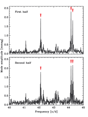
Figure 9: Fourier spectrum of CSTAR #n090586 derived using the Period04 program, based on data obtained during the first (top) and second (bottom) half of the 2010 season. Three significant peaks (at $f_{i}=44.288$, 44.169, and 42.121 cycles d^-1) are detected with varying amplitudes, which exhibit significant changes ($4-11\sigma$) relative to the 2008 season. See text for details.

The 2010 light curve of CSTAR#n057725 ($P=43.2$ d), originally discovered by the ASAS project (Pojmanski, 2005) and classified as a fundamental-mode $\delta$ Cephei variable, showed a dramatic change relative to 2008 as seen in Fig. 10. The Cepheid-like variability seen in the 2008 data (top-left panel), which already showed indications of a change in amplitude, decreased even further and developed a secondary peak in the 2010 data (top-right panel). Furthermore, eclipse-like events can now be seen at two distinct phases of the pulsation (bottom panels) separated by half of the period with depths of $\sim 0.07$ and $\sim 0.03$ mag. The $V$-band ASAS light curve, spanning more than a decade, also shows secular variations in pulsation amplitude. The ASAS classification of this object is very unlikely; at $i=10.1$ mag, a 43-day Cepheid would lie $\sim 17$ kpc away and nearly 8 kpc above the Galactic plane, an extremely improbable location for an $\sim 11M_{\odot}$ star. It is more likely that this object consists of a Population II pulsator, such as an RV Tauri or the Galactic equivalent of an OGLE small-amplitude variable red giant (Soszynski et al., 2004) in a binary system. We plan to undertake additional observations to investigate the nature of this system.

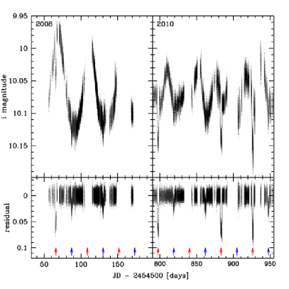
Figure 10: Light curve of CSTAR#n057725, showing the slow reduction in Cepheid-like pulsation amplitude during the 2008 season has been replaced by a more complex variability in 2010. Eclipse-like events seem to be present at two distinct phases indicated with red and blue arrows, respectively.

5 Conclusions and Summary

We have presented the analysis of high-cadence synoptic observations of 23 square degrees centered on the south celestial pole, conducted with the CSTAR#3 telescope at Dome A during 183 days of the 2010 Antarctic winter season. 86% of all frames obtained at a sun elevation angle below $0^{\circ}$ yielded useful data. We measured a median sky background of 19.8 mag $/\sq\arcsec$ over all moon phases and determined that the extinction is below 0.1 mag for 40% of the time (0.4 mag for 70% of the time). All these values are consistent with the site statistics derived from the 2008 season, and reinforce the promise of the Antarctic Plateau for future astronomical work.

We carried out time-series aperture photometry of 9,125 stars with $i<15.3$ mag. We detected $188$ variable stars, including $67$ new objects not included in our previous work thanks to a slightly larger field of view and a deeper magnitude limit. This represents a $\sim 4\times$ increase in the number of variable stars relative to previous surveys of the same region of the sky. We plan follow-up multi-wavelength photometry and high-resolution spectroscopy in the near future of the most interesting variables, such as detached eclipsing binaries and the candidate transiting exoplanets.

Given the coarse pixel scale of our images and our use of aperture photometry, the search for (non-periodic) variable stars was limited to objects with low levels of crowding. This could mitigated by the use of difference imaging techniques in future analyses. The apparent circular motion of stars in the field of view, due to the fixed nature of the telescope and camera, prevented the detection of periodic variability at frequencies close to one sidereal day (and its harmonics) despite the absence of a day/night cycle and the long duration of the observations. Future surveys conducted from Antarctica would greatly benefit from instruments with improved angular resolution, a finer pixel scale, and the ability to track. The recently-deployed AST3 telescopes (Cui et al., 2008) meets all these criteria and should greatly expand our synoptic capabilities in the polar regions.

Lingzhi Wang acknowledges support by: the BaiRen program of the Chinese Academy of Sciences (034031001); the National Natural Science Foundation of China under the Distinguished Young Scholar grant 10825313 and grants 11073005 & 11303041; the Ministry of Science and Technology National Basic Science Program (Project 973) under grant number 2012CB821804; the Excellent Doctoral Dissertation of Beijing Normal University Engagement Fund; and a Young Researcher Grant of the National Astronomical Observatories, Chinese Academy of Sciences.

Lucas Macri and Lifan Wang acknowledge support by the Department of Physics & Astronomy at Texas A&M University through faculty startup funds and the Mitchell-Heep-Munnerlyn Endowed Career Enhancement Professorship in Physics or Astronomy.

This work was supported by the Chinese PANDA International Polar Year project, NSFC-CAS joint key program through grant number 10778706, CAS main direction program through grant number KJCX2-YW-T08, and by the Chinese Polar Environment Comprehensive Investigation & Assessment Programmes (CHINARE). The authors deeply appreciate the great efforts made by the 24-28th Dome A expedition teams who provided invaluable assistance to the astronomers that set up and maintained the CSTAR telescope and the PLATO system. PLATO was supported by the Australian Research Council and the Australian Antarctic Division. Iridium communications were provided by the US National Science Foundation and the US Antarctic Program.

Facility: Dome A: CSTAR

References

- Ashley et al. (2010) Ashley, M. C. B., Allen, G., Bonner, C. S., Bradley, S. G., Cui, X., Everett, J. R., Feng, L., Gong, X., Hengst, S., Hu, J., Jiang, Z., Kulesa, C. A., Lawrence, J. S., Li, Y., Luong-Van, D. M., McCaughrean, M. J., Moore, A. M., Pennypacker, C., Qin, W., Riddle, R., Shang, Z., Storey, J. W. V., Sun, B., Suntzeff, N., Tothill, N. F. H., Travouillon, T., Walker, C. K., Wang, L., Yan, J., Yang, H., York, D. G., Yuan, X., Zhang, X., Zhang, Z., Zhou, X., & Zhu, Z. 2010, Highlights of Astronomy, 15, 627
- Burton (2010) Burton, M. G. 2010, A&A Rev., 18, 417
- Charbonneau et al. (2000) Charbonneau, D., Brown, T. M., Latham, D. W., & Mayor, M. 2000, ApJ, 529, L45
- Cui et al. (2008) Cui, X., Yuan, X., & Gong, X. 2008, in Society of Photo-Optical Instrumentation Engineers (SPIE) Conference Series, Vol. 7012, Society of Photo-Optical Instrumentation Engineers (SPIE) Conference Series
- Hartman et al. (2008) Hartman, J. D., Gaudi, B. S., Holman, M. J., McLeod, B. A., Stanek, K. Z., Barranco, J. A., Pinsonneault, M. H., & Kalirai, J. S. 2008, ApJ, 675, 1254
- Hengst et al. (2008) Hengst, S., Allen, G. R., Ashley, M. C. B., Everett, J. R., Lawrence, J. S., Luong-Van, D. M., & Storey, J. W. V. 2008, in Presented at the Society of Photo-Optical Instrumentation Engineers (SPIE) Conference, Vol. 7012, Society of Photo-Optical Instrumentation Engineers (SPIE) Conference Series
- Henry et al. (2000) Henry, G. W., Fekel, F. C., Henry, S. M., & Hall, D. S. 2000, ApJS, 130, 201
- Howell (2012) Howell, S. B. 2012, PASP, 124, 263
- Kaluzny et al. (1998) Kaluzny, J., Stanek, K. Z., Krockenberger, M., Sasselov, D. D., Tonry, J. L., & Mateo, M. 1998, AJ, 115, 1016
- Kenyon et al. (2006) Kenyon, S. L., Lawrence, J. S., Ashley, M. C. B., Storey, J. W. V., Tokovinin, A., & Fossat, E. 2006, PASP, 118, 924
- Kovács et al. (2002) Kovács, G., Zucker, S., & Mazeh, T. 2002, A&A, 391, 369
- Lawrence et al. (2008) Lawrence, J. S., Allen, G. R., Ashley, M. C. B., Bonner, C., Bradley, S., Cui, X., Everett, J. R., Feng, L., Gong, X., Hengst, S., Hu, J., Jiang, Z., Kulesa, C. A., Li, Y., Luong-Van, D., Moore, A. M., Pennypacker, C., Qin, W., Riddle, R., Shang, Z., Storey, J. W. V., Sun, B., Suntzeff, N., Tothill, N. F. H., Travouillon, T., Walker, C. K., Wang, L., Yan, J., Yang, J., Yang, H., York, D., Yuan, X., Zhang, X. G., Zhang, Z., Zhou, X., & Zhu, Z. 2008, in Presented at the Society of Photo-Optical Instrumentation Engineers (SPIE) Conference, Vol. 7012, Society of Photo-Optical Instrumentation Engineers (SPIE) Conference Series
- Lawrence et al. (2006) Lawrence, J. S., Ashley, M. C. B., Burton, M. G., Cui, X., Everett, J. R., Indermuehle, B. T., Kenyon, S. L., Luong-Van, D., Moore, A. M., Storey, J. W. V., Tokovinin, A., Travouillon, T., Pennypacker, C., Wang, L., & York, D. 2006, in Presented at the Society of Photo-Optical Instrumentation Engineers (SPIE) Conference, Vol. 6267, Society of Photo-Optical Instrumentation Engineers (SPIE) Conference Series
- Lawrence et al. (2009) Lawrence, J. S., Ashley, M. C. B., Hengst, S., Luong-Van, D. M., Storey, J. W. V., Yang, H., Zhou, X., & Zhu, Z. 2009, Rev Sci Instrum, 80, 064501
- Lenz & Breger (2005) Lenz, P. & Breger, M. 2005, Communications in Asteroseismology, 146, 53
- Lomb (1976) Lomb, N. R. 1976, Ap&SS, 39, 447
- Luong-Van et al. (2010) Luong-Van, D. M., Ashley, M. C. B., Cui, X., Everett, J. R., Feng, L., Gong, X., Hengst, S., Lawrence, J. S., Storey, J. W. V., Wang, L., Yang, H., Yang, J., Zhou, X., & Zhu, Z. 2010, in Presented at the Society of Photo-Optical Instrumentation Engineers (SPIE) Conference, Vol. 7733, Society of Photo-Optical Instrumentation Engineers (SPIE) Conference Series
- Mosser & Aristidi (2007) Mosser, B. & Aristidi, E. 2007, PASP, 119, 127
- Nugent et al. (2011) Nugent, P. E., Sullivan, M., Cenko, S. B., Thomas, R. C., Kasen, D., Howell, D. A., Bersier, D., Bloom, J. S., Kulkarni, S. R., Kandrashoff, M. T., Filippenko, A. V., Silverman, J. M., Marcy, G. W., Howard, A. W., Isaacson, H. T., Maguire, K., Suzuki, N., Tarlton, J. E., Pan, Y.-C., Bildsten, L., Fulton, B. J., Parrent, J. T., Sand, D., Podsiadlowski, P., Bianco, F. B., Dilday, B., Graham, M. L., Lyman, J., James, P., Kasliwal, M. M., Law, N. M., Quimby, R. M., Hook, I. M., Walker, E. S., Mazzali, P., Pian, E., Ofek, E. O., Gal-Yam, A., & Poznanski, D. 2011, Nature, 480, 344
- Ofek (2008) Ofek, E. O. 2008, PASP, 120, 1128
- Pojmanski (2005) Pojmanski, G. 2005, VizieR On-line Data Catalog: J/other/AcA/50.177. Originally published in: Acta Astron., 50, 177 (2001)
- Robin et al. (2003) Robin, A. C., Reylé, C., Derrière, S., & Picaud, S. 2003, A&A, 409, 523
- Samus et al. (2009) Samus, N. N., Durlevich, O. V., & et al. 2009, VizieR Online Data Catalog, 10, 2025
- Saunders et al. (2009) Saunders, W., Lawrence, J. S., Storey, J. W. V., Ashley, M. C. B., Kato, S., Minnis, P., Winker, D. M., Liu, G., & Kulesa, C. 2009, PASP, 121, 976
- Saunders et al. (2010) Saunders, W., Lawrence, J. S., Storey, J. W. V., Ashley, M. C. B., Kato, S., Minnis, P., Winker, D. M., Liu, G., & Kulesa, C. 2010, in EAS Publications Series, Vol. 40, EAS Publications Series, ed. L. Spinoglio & N. Epchtein, 89–96
- Scargle (1982) Scargle, J. D. 1982, ApJ, 263, 835
- Schlafly & Finkbeiner (2011) Schlafly, E. F. & Finkbeiner, D. P. 2011, ApJ, 737, 103
- Soszynski et al. (2004) Soszynski, I., Udalski, A., Kubiak, M., Szymanski, M., Pietrzynski, G., Zebrun, K., Szewczyk, O., & Wyrzykowski, L. 2004, Acta Astron., 54, 129
- Stellingwerf (1978) Stellingwerf, R. F. 1978, ApJ, 224, 953
- Stellingwerf (2011) Stellingwerf, R. F. 2011, in RR Lyrae Stars, Metal-Poor Stars, and the Galaxy, ed. A. McWilliam, 47
- Stetson (1987) Stetson, P. B. 1987, PASP, 99, 191
- Stetson (1996) —. 1996, PASP, 108, 851
- Storey (2009) Storey, J. W. 2009, Assoc Asia Pac Phys Soc Bull, 19, 4
- Storey (2005) Storey, J. W. V. 2005, Antarctic Science, 17, 555
- Storey (2007) —. 2007, Chinese Astron. Astrophys., 31, 98
- Tonry et al. (2005) Tonry, J. L., Howell, S. B., Everett, M. E., Rodney, S. A., Willman, M., & VanOutryve, C. 2005, PASP, 117, 281
- Udalski et al. (1994) Udalski, A., Szymanski, M., Stanek, K. Z., Kaluzny, J., Kubiak, M., Mateo, M., Krzeminski, W., Paczynski, B., & Venkat, R. 1994, Acta Astron., 44, 165
- Wang et al. (2011) Wang, L., Macri, L. M., Krisciunas, K., Wang, L., Ashley, M. C. B., Cui, X., Feng, L.-L., Gong, X., Lawrence, J. S., Liu, Q., Luong-Van, D., Pennypacker, C. R., Shang, Z., Storey, J. W. V., Yang, H., Yang, J., Yuan, X., York, D. G., Zhou, X., Zhu, Z., & Zhu, Z. 2011, AJ, 142, 155
- Yang et al. (2009) Yang, H., Allen, G., Ashley, M. C. B., Bonner, C. S., Bradley, S., Cui, X., Everett, J. R., Feng, L., Gong, X., Hengst, S., Hu, J., Jiang, Z., Kulesa, C. A., Lawrence, J. S., Li, Y., Luong-Van, D., McCaughrean, M. J., Moore, A. M., Pennypacker, C., Qin, W., Riddle, R., Shang, Z., Storey, J. W. V., Sun, B., Suntzeff, N., Tothill, N. F. H., Travouillon, T., Walker, C. K., Wang, L., Yan, J., Yang, J., York, D., Yuan, X., Zhang, X., Zhang, Z., Zhou, X., & Zhu, Z. 2009, PASP, 121, 174
- Young (1967) Young, A. T. 1967, AJ, 72, 747
- Yuan et al. (2008) Yuan, X., Cui, X., Liu, G., Zhai, F., Gong, X., Zhang, R., Xia, L., Hu, J., Lawrence, J. S., Yan, J., Storey, J. W. V., Wang, L., Feng, L., Ashley, M. C. B., Zhou, X., Jiang, Z., & Zhu, Z. 2008, in Society of Photo-Optical Instrumentation Engineers (SPIE) Conference Series, Vol. 7012, Society of Photo-Optical Instrumentation Engineers (SPIE) Conference Series
- Zhou et al. (2010a) Zhou, X., Fan, Z., Jiang, Z., Ashley, M. C. B., Cui, X., Feng, L., Gong, X., Hu, J., Kulesa, C. A., Lawrence, J. S., Liu, G., Luong-Van, D. M., Ma, J., Moore, A. M., Qin, W., Shang, Z., Storey, J. W. V., Sun, B., Travouillon, T., Walker, C. K., Wang, J., Wang, L., Wu, J., Wu, Z., Xia, L., Yan, J., Yang, J., Yang, H., Yuan, X., York, D., Zhang, Z., & Zhu, Z. 2010a, PASP, 122, 347
- Zhou et al. (2010b) Zhou, X., Wu, Z., Jiang, Z., Cui, X., Feng, L., Gong, X., Hu, J., Li, Q., Liu, G., Ma, J., Wang, J., Wang, L., Wu, J., Xia, L., Yan, J., Yuan, X., Zhai, F., Zhang, R., & Zhu, Z. 2010b, Research in Astronomy and Astrophysics, 10, 279
- Zou et al. (2010) Zou, H., Zhou, X., Jiang, Z., Ashley, M. C. B., Cui, X., Feng, L., Gong, X., Hu, J., Kulesa, C. A., Lawrence, J. S., Liu, G., Luong-Van, D. M., Ma, J., Moore, A. M., Pennypacker, C. R., Qin, W., Shang, Z., Storey, J. W. V., Sun, B., Travouillon, T., Walker, C. K., Wang, J., Wang, L., Wu, J., Wu, Z., Xia, L., Yan, J., Yang, J., Yang, H., Yao, Y., Yuan, X., York, D. G., Zhang, Z., & Zhu, Z. 2010, AJ, 140, 602