Cooperative Topology Control with Adaptation for Improved Lifetime
in Wireless Sensor Networks

Abstract

Topology control algorithms allow each node in a wireless multi-hop network to adjust the power at which it makes its transmissions and choose the set of neighbors with which it communicates directly, while preserving global goals such as connectivity or coverage. This allows each node to conserve energy and contribute to increasing the lifetime of the network. In this paper, in contrast to most previous work, we consider (i) both the energy costs of communication as well as the amount of available energy at each node, (ii) the realistic situation of varying rates of energy consumption at different nodes, and (iii) the fact that co-operation between nodes, where some nodes make a sacrifice by increasing energy consumption to help other nodes reduce their consumption, can be used to extend network lifetime. This paper introduces a new distributed topology control algorithm, called the Cooperative Topology Control with Adaptation (CTCA), based on a game-theoretic approach that maps the problem of maximizing the network’s lifetime into an ordinal potential game. We prove the existence of a Nash equilibrium for the game. Our simulation results indicate that the CTCA algorithm extends the life of a network by more than 50% compared to the best previously-known algorithm. We also study the performance of the distributed CTCA algorithm in comparison to an optimal centralized algorithm as a function of the communication ranges of nodes and node density.

I Introduction

In wireless ad hoc networks, especially ad hoc sensor networks, the battery life of each node plays a critical role in determining the functional lifetime of the entire network. When a node exhausts its limited energy supply, it may fail to reach nearby nodes leading to a disconnected network and disabling some essential communications. Without energy, the node will also fail to continue the environmental monitoring activities essential to the functional operation of the system. Adding redundant nodes in the network may extend the functional lifetime but it is ultimately a less cost-effective approach. In this paper, we consider the problem of extending the lifetime of a network using a new adaptive game-theoretic approach.

Topology control is among the better-known approaches to conserving energy and prolonging a network’s functional life. In a topology control algorithm, each node adjusts the power at which it makes its transmissions to reduce the energy consumption to only what is needed to ensure topological goals such as connectivity or coverage. Examples of topology control algorithms include Directed Relative Neighborhood Graph (DRNG) [1], Directed Local Spanning Subgraph (DLSS) [1], Step Topology Control (STC) [2] and Routing Assisted Topology Control (RATC) [3]. In most traditional algorithms, the topology of the network is determined at the very beginning of the life of the network where the only consideration for each node is to reduce its transmission power while keeping the graph connected. After the execution of one of these algorithms, each node will transmit at the selected power level until it eventually runs out of energy. However, depending on the location of a node in relation to others, some nodes may end up with a much larger communication radius, and therefore a much larger transmission power, than some others. This uneven distribution of the assigned transmission powers may result in an unbalanced energy consumption at the nodes, leading to some nodes exhausting their energy far sooner than some others. Such a scenario can end the functional life of the network earlier than necessary. This highlights two weaknesses of these algorithms: they are not adaptive to different rates of energy consumption on different nodes and they do not allow cooperation between nodes to extend the network lifetime. Each of these weaknesses is addressed by the algorithm proposed in this paper: Cooperative Topology Control with Adaptation (CTCA).

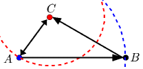
(a) The initial topology of the network where no node can reduce its transmission power.

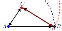
(b) Node $C$ chooses to increase its transmission power so as to directly connect to $B$.

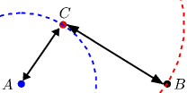
(c) Node $A$ can now reduce its transmission power to directly connect only to $C$.

Figure 1: An example illustrating cooperative topology control.

We illustrate the principle of cooperative topology control with a simple toy example shown in Fig. 1. Suppose Fig. 1(a) illustrates the result of a topology control algorithm, where no node can reduce its transmission power unilaterally without disconnecting the graph. In this figure, the presence of an edge from one node, say $A$, to another node, say $B$, implies that $A$ can transmit at a power level sufficient to reach node $B$. The communication radius of each node is shown by the dashed arcs. Assuming all nodes start out with the same energy supply and make transmissions at the same rate, we note that node $A$ has the largest energy cost and thus has the shortest lifetime. Node $C$, on the other hand, has the smallest transmission power, and therefore, has the longest lifetime. Traditional topology control algorithms discussed above will lead to the situation in Fig. 1(a) ending the functional life of the network when node $A$’s energy is exhausted even though node $C$ would have plenty of remaining energy. Fig. 1(b) illustrates a topology where node $C$ increases its transmission power so that it can now reach node $B$ directly. Now, node $A$ is able to reduce its transmission power to only be directly connected to node $C$, as shown in Fig. 1(c). This involves node $C$ making a sacrifice by increasing the power at which it makes its transmissions in order to allow node $A$ to reduce its transmission power, thus extending the life of node $A$ and of the network.

The actual power consumption for sending and receiving a data packet varies significantly depending on the radio environment of the space where the sensor nodes are located and also the electronics of the devices. The log-distance path loss model based on the path loss as a logarithmic function of the distance $d$ has been confirmed both theoretically and by measurements in a large variety of environments [4, 5, 6]. In this model, the path loss at distance $d$, $PL(d)$ is expressed as:

$$PL(d)=PL(d_{0})+10\gamma\log_{10}(d/d_{0})$$

where the constant $d_{0}$ is an arbitrary reference distance and $\gamma$ is called the path loss exponent. This implies that the energy consumed to make a transmission across a distance $d$ is proportional to $d^{\gamma}$. Since $\gamma$ ranges from 2.5 to 6 in most real environments [4], especially over longer distances, a single transmission over distance $d$ often consumes more energy than two transmissions each over distance $d/2$. This motivates the goal of most topology control algorithms to choose multiple smaller hops in place of a single longer hop with the intent to reduce overall energy consumption. While device electronics can sometimes be such that choosing smaller hops—especially at smaller distances—does not always guarantee lower energy consumption, there is another good reason to choose smaller hops: reducing interference in all communications. Therefore, a general goal of a topology control algorithm is to achieve lower transmission powers for all the sensor nodes in order to reduce both energy consumption and interference [7]. In other words, the topology illustrated in Fig. 1(c) is more desirable.

In this paper, we employ game theory to facilitate such topology control that allows cooperation between nodes as illustrated in Fig. 1. Our approach is through developing an ordinal potential game [8, 3, 9] into which our problem can be mapped, so that all nodes pursue a localized strategy that can be expressed through a single global function, or the global potential function. Our approach also allows an adaptive strategy so that a node does not end up with the same power level through its entire lifetime. This is significant to extending the network lifetime because it is almost always the case that different nodes consume energy at different rates. Our approach to allowing adaptation is through incorporating the energy remaining on the nodes in the neighborhood into the decisions made by each node. Since this remaining energy changes over the life of a network, our topology control algorithm adaptively adjusts the power levels at each node. This constantly keeps shifting energy consumption from nodes with less energy reserves to those with more energy reserves, thus extending the life of the network.

I-A Problem Statement

Given a wireless sensor network, let graph $G(t)=(N,E(t))$ represent its topology at time $t$, where $N_{i}\in N$ represents a node within the network, and $(N_{i},N_{j})\in E(t)$ represents the fact that node $N_{j}$ is within node $N_{i}$’s communication radius and can hear from $N_{i}$ directly at time $t$. Assume $G(t)$ is a connected graph at time $t$. Topology control algorithms have traditionally emphasized preserving connectivity as a constraint while pursuing the goal of reduced energy consumption at each node.

However, depending on the type of application for which an ad hoc sensor network is deployed, it is possible that a network is functional even if a certain subset of nodes runs out of energy [10, 11, 12]. The functional lifetime of a network, therefore, depends on the application in use and consequently, there is some debate on how best to define the functional lifetime of a network. In an ad hoc sensor network with a non-hierarchical topological organization, one may assume an application-dependent parameter, $c$, to define the functional lifetime as the length of time the network topology possesses at least one connected component with $n-c$ or more nodes (where $n$ is the total number of nodes in the network). When $c=0$, the functional lifetime of the network is the length of time $G(t)$ is a connected graph, which is until any node is disconnected or runs out of energy.

We find that a definition of functional lifetime using $c=0$ is a more versatile one for two reasons: firstly, on any application, there may be some crucial nodes which, when they die, can disable the functionality of the network; secondly, a definition based on the $c=0$ case can form the foundation of greedy algorithms designed to extend functional lifetime for $c>0$.

In this paper, therefore, we consider the functional life of the network to have ended when one of the following two cases occurs:

• Case 1: A node reduces its current transmission power in order to save energy, but becomes unable to reach certain nodes and, consequently, loses connection from part of the network.

• Case 2: A node runs out of energy, thus getting disconnected from the rest of the network.

If Case 1 happens, the communication links whose removal caused the network to become disconnected can be restored back into the network to restore the functional life of the network. On the other hand, if Case 2 happens, the network’s functional lifetime cannot be extended in any way. Therefore, to improve the lifetime of the network, (i) Case 1 should be avoided by always ensuring connectivity in the assignment of power levels to the nodes, and (ii) Case 2 should be pushed as far into the future as possible by reducing the rate of energy consumption at the node that is estimated to have the smallest remaining lifetime. The problem can now be defined as one of periodically reassigning the power at which each node makes its transmissions so that the first occurrence of either Case 1 or Case 2 is pushed as far ahead in time as possible.

I-B Contributions and Organization

Section II reviews the related work on approaches that have been employed to increase a wireless sensor network’s lifetime through topology control. Section III analyzes the rationale behind the approach used in this paper and presents a few definitions and lays out the foundational concepts for the game-theoretic approach used in this paper. Section IV proves the existence of a Nash equilibrium for the ordinal potential game used to map our problem. Our proof is based on showing that the difference in individual payoffs for each node from unilaterally changing its strategy and the difference in values of the global potential function have the same sign.

The pseudo-code for the Cooperative Topology Control with Adaptation (CTCA) algorithm is presented in Section V. A simulation-based evaluation of its performance and a comparative analysis with other topology control algorithms are described in Section VI. Our results show that the CTCA algorithm extends the life of a network by more than 50% compared to the best previously-known algorithm. This section also compares the topology delivered by the distributed CTCA algorithm to the optimal solution obtained using a centralized algorithm. We also study the dependence of the performance of CTCA in relation to the optimal on the communication ranges of nodes and on the node density.

Section VII concludes the paper.

II Related Work

The task of extending the life of a wireless sensor network can be tackled through multiple complementary ways involving routing protocols, medium access strategies or any of several other protocols that facilitate network operations. In this section, we will discuss only the approaches most related to this paper; that is, approaches based on changing the topology of the network by individual nodes changing the power levels at which they make their transmissions while preserving network connectivity.

Traditional topology control algorithms such as Small Minimum-Energy Communication Network (SMECN)[13], Minimum Spanning Tree (MST) [14], DRNG[1], DLSS[1] and STC[2] usually start the topology control process with each node transmitting at its maximum transmission power to discover all of its neighbors. Local neighborhood and power-level information is next exchanged between neighbors. The minimum transmission power of each node such that the graph is still connected is later computed at each node without further communication between nodes. The Weighted Dynamic Topology Control (WDTC) [15] algorithm improves upon the work of MST, and considers the remaining energy of each node in addition to the energy cost of communication across each pair of nodes. The algorithm, however, forces bidirectional communication between each pair of nodes and, in addition, requires periodic communication by each node at its maximum possible power level. Other related algorithms seek to offer a robust topology where the graph can stand multiple channel failures; for example, a $k$-connected graph is sought in [16, 17] and a two-tiered network in [18].

Other topology control algorithms may require communication between nodes throughout the topology control process. One typical example is the work described in [19], which is based on a selfish game on network connectivity to help reduce the transmission power on each node. By offering a utility function which indicates a high profit if the node’s transmission power is small and a low profit if the node’s transmission power is large, each node selfishly reduces its transmission power to maximize its profit. On the other hand, if the node has reduced its transmission power to such an extent that the graph becomes disconnected, the profit of each node becomes 0. This algorithm was later improved in [3], where the requirement of global information (to establish connectivity) is eliminated and a distributed topology control algorithm is proposed. Among the first works on using game theory in topology control problems is [20] which gives tight bounds on worst-case Nash equilibria for a game in which the network is required to preserve connectivity. However, this study only considers selfish nodes which try to minimize their energy consumption without considering potential sacrifices nodes can make (by expending more energy) to extend a network’s lifetime.

Another class of topology control algorithms is represented by the work reported in [21], where the authors provide a decentralized static complete-information game for power scheduling, considering both frame success rate and connectivity. Yet other approaches to increasing the lifetime of a wireless sensor network include grouping nodes into clusters to create a communication hierarchy in which nodes in a cluster communicate only with their cluster head and only cluster heads are allowed to communicate with other cluster heads or the sink node [22, 23, 24, 25, 26, 27]. In the work of [28], the authors tried to assign sensor nodes with different initial energy levels so that sensor nodes with high traffic load will be assigned more energy than those with smaller loads. By doing so, with the same amount of overall energy, the network’s lifetime may be extended.

If the network’s lifetime is measured in terms of how many transmissions can be made before the sensor nodes run out of energy, then maximizing the network’s lifetime can be interpreted as maximizing the throughput of the network. In the work of [29], the authors studied the relationship between throughput of the network and its corresponding lifetime under an SINR model. But they focus on a specific network setting where sensor nodes’ neighbors and the communication links are predetermined and the topology of the network remains constant throughout the network’s lifetime.

A survey of topology control algorithms can be found in [30, 31] and a survey of the applications of game theory in wireless sensor networks can be found in [32, 33].

The CTCA algorithm proposed in this paper is the first to use a game-theoretic approach that also adapts to changes in the remaining energy levels of nodes and which allows co-operative behavior amongst nodes. As will be discussed in the following sections, these features allow it to extend the life of a network by more than 50% compared to the best previously-known algorithm.

III Definitions and Preliminaries

In this section, we define terms and concepts that will enable us to specify the localized goals that each node should pursue in order to achieve the global goal of increased lifetime for the network.

Let $W_{i}(t)$ denote the amount of energy remaining at node $N_{i}$ at time $t$. Let $p_{i}(t)$ denote the power at which node $N_{i}$ makes its transmissions at time $t$. As an estimate of the additional length of time before a node runs out of energy, we define the estimated lifetime of node $N_{i}$ at time $t$, denoted by $L_{i}(p_{i}(t),t)$, as the ratio between the amount of remaining energy on the node at time $t$ and the power at which it makes its transmissions at time $t$. That is, $L_{i}(p_{i}(t),t)=W_{i}(t)/p_{i}(t)$. Note that the estimated lifetime may or may not accurately capture the actual remaining lifetime of a node (because its transmission powers may change later or its energy reserves may deplete slower/faster than estimated.) When the context is clear, for brevity, we refer to the estimated lifetime as just the lifetime.

In a system in which the rate of energy consumption is largely balanced across the nodes (which is the goal of this paper as a means to improve network lifetime), the node with the smallest estimated lifetime is likely the one that determines the network’s lifetime. We consider the estimated lifetime of a network as the estimated lifetime of the node with the smallest estimated lifetime. If $N_{i}$ is the node with the smallest estimated lifetime within the network, then it may be possible to improve the network’s lifetime by improving $N_{i}$’s estimated lifetime. Fig. 1 shows an example where node $A$ is able to reduce its transmission power with help from node $C$, thus increasing its estimated lifetime and likely the lifetime of the network.

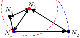
(a) Node $N_{3}$’s initial state, where node $N_{1}$ is not capable of reducing its transmission power without disconnecting the graph.

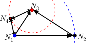
(b) Situation 1: Node $N_{3}$ reduces its transmission power to its potential transmission power, but $N_{1}$’s lifetime cannot be improved.

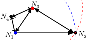
(c) Situation 2: Node $N_{3}$ increases its transmission power to $p(N_{3},N_{2})$. Now, node $N_{1}$ is able to reduce its power without disconnecting the graph.

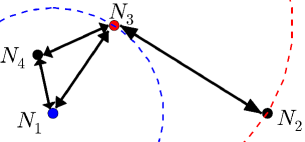
(d) Node $N_{1}$ updates its current transmission power to its potential transmission power, and extends its lifetime and of the network.

Figure 2: An example illustrating how a node should choose its power level so as to increase the network’s lifetime.

We further illustrate the definitions in this section using the topology shown in Fig. 2. Suppose at time $t$, the topology of the network is as shown in Fig. 2(a). Denote by $p(N_{i},N_{j})$ the minimum transmission power at which nodes $N_{i}$ and $N_{j}$ have to transmit to reach each other. We refer to the set of transmission powers that a node may switch to at time $t$ as its available transmission powers at time $t$. Then, according to the topology given by Fig. 2(a), node $N_{3}$’s available transmission powers are: $p(N_{3},N_{1})$, $p(N_{3},N_{2})$ and $p(N_{3},N_{4})$, while its current transmission power is $p(N_{3},N_{1})$ (note that there is no need for node $N_{3}$ to transmit at any power level other than the ones in this available set).

Let $\mathbf{P}$ denote a mapping of nodes in the network to power levels. For example, in Fig. 2(a), the mapping implemented is given by $\mathbf{P}=\{\,N_{1}\rightarrow p(N_{1},N_{2}),N_{2}\rightarrow p(N_{2},N_{3}),N_{3}\rightarrow p(N_{3},N_{1}),N_{4}\rightarrow p(N_{4},N_{3})\,\}$. Since node $N_{3}$ has the potential to transmit at power $p(N_{3},N_{4})$ while still keeping the graph connected, we refer to power $p(N_{3},N_{4})$ as node $N_{3}$’s potential transmission power under this node-to-power mapping $\mathbf{P}$.

In general, the potential transmission power of a node is the smallest available transmission power that the node can use such that the graph is still connected while the power levels at all other nodes remain the same. Let $p^{\prime}_{i}(\mathbf{P})$ denote the potential transmission power of node $N_{i}$ under the node-to-power mapping $\mathbf{P}$. Note that a node’s potential transmission power is no greater than its current transmission power provided that the network is currently connected. That is, $p^{\prime}_{i}(\mathbf{P})\leq p_{i}(t)$ if $G(t)$ is a connected graph and $\mathbf{P}$ is the node-to-power mapping implemented at time $t$.

Transmitting at the potential transmission power as defined above can increase the lifetime of a node beyond its estimated lifetime and, consequently, of the network. To estimate the best lifetime a node can achieve without changing the transmission powers of other nodes and without disconnecting the network, we define the potential lifetime of a node as the ratio between the node’s current remaining energy and its potential transmission power. Let $L^{\prime}_{i}(\mathbf{P},t)$ denote the potential lifetime of node $N_{i}$ at time $t$ under the node-to-power mapping $\mathbf{P}$. Let $p^{\prime}_{i}(\mathbf{P})$ denote its potential transmission power under the node-to-power mapping $\mathbf{P}$. Then, $L^{\prime}_{i}(\mathbf{P},t)=W_{i}(t)/p^{\prime}_{i}(\mathbf{P})$.

If $p^{\prime}_{i}(\mathbf{P})\leq p_{i}(t)$, then $L_{i}(p_{i}(t),t)\leq L^{\prime}_{i}(\mathbf{P},t)$. Therefore, to increase its estimated lifetime, a node should always try to change its current transmission power to its potential transmission power, if they are not the same. Figs. 2(a) and 2(b) illustrate such a process for node $N_{3}$, where it changes its current transmission power from $p(N_{3},N_{1})$ in Fig. 2(a) to its potential transmission power $p(N_{3},N_{4})$ as illustrated in Fig. 2(b).

In Fig. 2(a), suppose node $N_{1}$ is the node that has the smallest estimated lifetime within the network. Then, $N_{1}$’s estimated lifetime has to be improved in order to improve the network’s lifetime. In Fig. 2(b), node $N_{3}$ reduces its transmission power but this does not improve the potential lifetime of node $N_{1}$. This implies that $N_{1}$’s estimated lifetime cannot be improved by node $N_{3}$ reducing its transmission power. On the other hand, if node $N_{3}$ chooses to transmit at a higher power level, $p(N_{3},N_{2})$, as illustrated in Fig. 2(c), then node $N_{1}$’s potential transmission power reduces to $p(N_{1},N_{3})$. Now, node $N_{1}$ can reduce its transmission power to the new potential transmission power as illustrated in Fig. 2(d), thus improving the network’s estimated lifetime.

Let $R_{i}(t)$ denote the set of nodes $N_{i}$ can reach at time $t$; i.e., $R_{i}(t)=\{N_{j}\,|\,p(N_{i},N_{j})\leq p_{i}(t)\}$. Let $I_{i}(t)$ denote the set of nodes that can reach node $N_{i}$ at time $t$, i.e, $I_{i}(t)=\{N_{j}\,|\,p(N_{j},N_{i})\leq p_{j}(t)\}$. Then for any $N_{j}\in I_{i}(t)$, we have $N_{i}\in R_{j}(t)$. We refer to the nodes in the set $R_{i}(t)$ as the reachable neighbors of node $N_{i}$ and the nodes in the set $I_{i}(t)$ as the reverse-link neighbors of $N_{i}$. For example, in Fig. 2(a), $N_{1}$’s reachable neighbors are $N_{2}$, $N_{3}$ and $N_{4}$ while $N_{2}$ has only one reachable neighbor, $N_{3}$. Also, $N_{1}$ is a reverse-link neighbor of $N_{2}$, $N_{3}$ and $N_{4}$. Let $H_{i}(t)=R_{i}(t)\cup N_{i}$ and let $O_{i}(t)=I_{i}(t)\cup N_{i}$.

In Fig. 2(a), note that $N_{1}$’s potential transmission power will not be reduced unless either $N_{3}$ or $N_{4}$ has increased its transmission power to be able to reach $N_{2}$. In general, $N_{i}$’s reachable neighbors are the only nodes who can help $N_{i}$ reduce its potential transmission power; and only the nodes who are $N_{i}$’s reverse-link neighbors may benefit from $N_{i}$’s increase in its transmission power level.

A question worth answering at this point is about what might be the relationship between improving the network’s lifetime and improving node $N_{1}$’s estimated and potential lifetime. As we have stated previously, the network’s estimated lifetime is dependent upon the node with the smallest estimated lifetime. If we compare the power mapping illustrated in Fig. 2(a) and Fig. 2(d), we can see that node $N_{3}$ not only has sacrificed its chance to improve its lifetime but also has sacrificed its own estimated lifetime (increases its current transmission power from $p(N_{3},N_{1})$ to $p(N_{3},N_{2})$) in order to help improve node $N_{1}$’s potential lifetime which is the smallest in Fig. 2(a). When the topology is as illustrated in Fig. 2(d), suppose node $N_{3}$ is the node with the smallest estimated lifetime. If its estimated lifetime in the topology illustrated in Fig. 2(d) is less than that of node $N_{1}$’s in the topology illustrated in Fig. 2(a), the network’s estimated lifetime in fact reduces rather than increases. In such a case, node $N_{3}$ should not choose to increase its transmission power to help improve $N_{1}$’s lifetime, but should instead focus on improving its own estimated lifetime.

For any node $N_{i}$ within the graph, its estimated lifetime will not improve unless it switches to its potential transmission power. That is to say, no node can help node $N_{i}$ with its estimated lifetime except for node $N_{i}$ itself; but as illustrated in Fig. 2, another node may help with $N_{i}$’s potential lifetime. In our example, node $N_{3}$ helps node $N_{1}$ improve its potential lifetime which eventually allows $N_{1}$ to increase its estimated lifetime by changing its transmission power to the potential transmission power.

The above discussion leads to the following primary and secondary goals for each node in order to improve the network’s lifetime while also conserving energy as much as possible:

• Primary goal: Let $m(i)$ denote the node with the smallest potential lifetime amongst the reverse-link neighbors of node $N_{i}$. Let $q$ denote the potential lifetime of node $m(i)$. The primary goal of node $N_{i}$ should be to increase the potential lifetime of node $m(i)$ above $q$ while making sure that its own estimated lifetime does not reduce below $q$.

• Secondary goal: The secondary goal of node $N_{i}$ should be to increase its own estimated lifetime.

The secondary goal is achieved once a node adopts its potential transmission power as its current transmission power (in this situation, its potential lifetime then becomes its estimated lifetime). Note that, if the primary and the secondary goals conflict, a node should always choose to meet the primary goal. This leads us into the design of the cooperative game that each node can play with its reachable neighbors and its reverse-link neighbors.

One may argue that since the ultimate goal is to extend functional lifetime (the primary goal), the secondary goal should be unnecessary. However, there are three reasons why we include the secondary goal in our design of the algorithm.

Firstly, for any realistic algorithm, it is not possible to precisely predict the network lifetime since it is not possible to predict with precision the future traffic load experienced by any given sensor node. As a result, an algorithm can only seek to maximize the estimated functional lifetime of a node and not the actual functional lifetime. Therefore, the secondary goal helps each sensor node save energy as much as possible so that when the estimated functional lifetime deviates from the actual functional lifetime, the node that actually determines the network’s functional lifetime (the one that dies earliest) does not waste any energy by transmitting at a power larger than what was necessary to stay connected. Secondly, as discussed in Section I-A, we define the functional lifetime assuming $c=0$. However, if the functional lifetime for some application is defined assuming that the network function survives until $c>0$ nodes are disconnected, a good heuristic for extending the functional lifetime emerges if we implement the secondary goal in conjunction with the primary goal assuming $c=0$ on the surviving largest connected component every time a node dies. Thirdly, reducing the transmission power of a sensor node may help reduce the interference among transmissions, reducing retransmissions and also helping extend the functional lifetime of the network.

In the above discussion, without loss of generality, we assume that there is only one node $m(i)$ with the smallest potential lifetime amongst reverse-link neighbors of $N_{i}$. If there is a tie with two nodes having identical potential lifetimes, one can always break the tie in the algorithm using a consistently applied second criterion such as the node id.

IV The Ordinal Potential Game

In this section, we present the notation and the utility function governing the ordinal potential game into which we map the problem of extending the lifetime of the network.

IV-A Notation

Table I presents a glossary of terms used in this section. In this paper, for brevity and clarity, we sometimes omit the time index $t$ whenever the corresponding instant of time is clear from the context.

TABLE I: A glossary of selected terms. If the time $t$ specified within each notation is clear within the context, it is omitted for purposes of brevity. In the glossary, however, we list each notation in both forms (with and without $t$).

Notation	Definition
$N$	The set of $n$ nodes within the network. $N=\{N_{1},N_{2},...,N_{n}\}$.
$G(t)$	Graph representing the network topology at time $t$. $G(t)=(N,E(t))$
$p_{i}(t)$ or $p_{i}$	Node $N_{i}$’s transmission power at time $t$.
$\mathbf{P}$	A mapping, $\mathbf{P}:N\rightarrow\mathbb{R}$, of the nodes in the network to transmission power levels. For example, the mapping actually implemented at time $t$ is $\{N_{1}\rightarrow p_{1}(t),N_{2}\rightarrow p_{2}(t),\dots\}$
$\mathbf{P}_{-i}$	A mapping of all the nodes except $N_{i}$ to transmission power levels.
$p(N_{i},N_{j})$	The minimum transmission power needed for node $N_{i}$’s transmissions to reach node $N_{j}$. We assume $p(N_{i},N_{j})=p(N_{j},N_{i})$.
$R_{i}(t)$ or $R_{i}$	The set of nodes reachable by $N_{i}$’s transmissions at time $t$. $R_{i}(t)=\{N_{j}\,|\,(N_{i},N_{j})\in E(t)\}$. This set of reachable neighbors is also called the reachable neighborhood of $N_{i}$.
$H_{i}(t)$ or $H_{i}$	The set including $N_{i}$ and its reachable neighbors. $H_{i}(t)=R_{i}(t)\cup N_{i}$.
$I_{i}(t)$ or $I_{i}$	The set of nodes at time $t$ which can directly reach $N_{i}$ with their transmissions. $I_{i}(t)=\{N_{j}\,|\,(N_{j},N_{i})\in E(t)\}$. This set of reverse-link neighbors of $N_{i}$ is also called reverse-link neighborhood of $N_{i}$.
$O_{i}(t)$ or $O_{i}$	The set including $N_{i}$ and its reverse-link neighbors. $O_{i}(t)=I_{i}(t)\cup N_{i}$.
$\mathbf{P}_{i}$	A mapping, $\mathbf{P}_{i}:H_{i}\rightarrow\mathbb{R}$, of $N_{i}$ and its reachable neighbors to transmission power levels.
$\mathbf{P}_{i,-j}$	A mapping of $N_{i}$ and its reachable neighbors except $N_{j}$ to transmission power levels.
$p^{\prime}_{i}(\mathbf{P}_{i})$	$N_{i}$’s potential transmission power when its and its reachable neighbors’ power levels are given by the mapping $\mathbf{P}_{i}$.
$A_{i}$	$N_{i}$’s possible transmission power choices.
$W_{i}(t)$ or $W_{i}$	$N_{i}$’s remaining energy at time $t$.
$L_{i}(a_{i},t)$	$N_{i}$’s estimated lifetime (remaining) at time $t$ if set to transmit at power $a_{i}$. $L_{i}(a_{i},t)=W_{i}(t)/a_{i}$
$L^{\prime}_{i}(\mathbf{P}_{i},t)$	$N_{i}$’s potential lifetime at time $t$ when its and its reachable neighbors’ transmission powers are given by the mapping $\mathbf{P}_{i}$. $L^{\prime}_{i}(\mathbf{P}_{i},t)=W_{i}(t)/p^{\prime}_{i}(\mathbf{P}_{i})$
$m(i,t)$ or $m(i)$	The node with the smallest potential lifetime among $N_{i}$’s reverse-link neighbors at time $t$. $m(i,t)=arg\min_{N_{j}\in I_{i}(t)}(L^{\prime}_{j}(\mathbf{P}_{j},t))$.

Suppose that at time $t=0$, each node is transmitting at its maximum transmission power $p_{\text{max}}$. Then, the set of nodes that includes $N_{i}$’s reachable neighbors is $R_{i}(0)=\{N_{j}\,|\,p(N_{i},N_{j})\leq p_{\text{max}}\}$. Let $n_{i}$ denote the size of the set $R_{i}(0)$. Therefore, we define the available transmission powers for node $N_{i}$ as $A_{i}=\{p_{i}^{1},p_{i}^{2},\dots,p_{i}^{n_{i}}\}$ where, for any $p_{i}^{k}\in A_{i}$, there exists a node $N_{j}\in R_{i}(0)$ such that $p_{i}^{k}$ is the minimum transmission power required for $N_{i}$ to reach $N_{j}$. Note that a node does not need to transmit at power levels other than the ones needed to reach other nodes within its maximum range.

Let $\mathbf{P}$ denote a mapping of the nodes in the network to transmission power levels. The mapping implemented at time $t$ is $\mathbf{P}=\{\,N_{i}\rightarrow p_{1}(t),N_{2}\rightarrow p_{2}(t),\dots\}$, where $p_{i}(t)$ is the power at which node $N_{i}$ is set to make transmissions at time $t$. We write $\mathbf{P}=\{\,f_{i},\mathbf{P}_{-i}\,\}$ where $f_{i}$ is a mapping of node $N_{i}$ to a certain power level and $\mathbf{P}_{-i}$ is a mapping of all other nodes in the network to power levels.

Let $\mathbf{P}_{i}$ denote a mapping, $\mathbf{P}_{i}:H_{i}\rightarrow\mathbb{R}$, of $N_{i}$ and its reachable neighbors to power levels. We write $\mathbf{P}_{i}=\{\,f_{j},\mathbf{P}_{i,-j}\,\}$ where $f_{j}$ is a mapping of node $N_{j}\in H_{i}$ to a certain power level and $\mathbf{P}_{i,-j}$ is a mapping of all other nodes in $H_{i}$ to power levels.

Let $L_{i}(a_{i},t)$ denote the estimated lifetime of node $N_{i}$ at time $t$ if set to transmit at power level $a_{i}$. Per the definition of estimated lifetime, $L_{i}(a_{i},t)=W_{i}(t)/a_{i}$. If $a_{i}=p^{\prime}_{i}(\mathbf{P}_{i})$, then $L_{i}(a_{i},t)=L^{\prime}_{i}(\mathbf{P}_{i},t)$.

Denote by $m(i,t)$, or $m(i)$ for brevity, the node in $I_{i}(t)$ with the smallest potential lifetime. We define the potential lifetime of $N_{i}$’s reverse-link neighborhood at time $t$ as the potential lifetime of node $m(i)$ at time $t$, i.e., $L^{\prime}_{m(i)}(\mathbf{P}_{m(i)},t)$.

IV-B The utility function

In the following, we present and justify the utility function governing the ordinal potential game upon which our topology control algorithm is based.

As stated in Section III, the primary goal for each sensor node is to improve the potential lifetime of its reverse-link neighborhood without also causing a reduction in the network’s estimated lifetime. While prioritizing the primary goal, the secondary goal of the sensor node is to improve its own estimated lifetime. Both of these goals are captured in the utility function presented in this section.

Let $a_{i}\in A_{i}$ denote a power level that is available to node $N_{i}$ at time $t$. Define the primary utility function (corresponding to the primary goal described in Section III) for node $N_{i}$ with power level $a_{i}$ at time $t$ as:

$$u_{i}^{X}(a_{i},t) =\min\left(\min_{N_{j}\in I_{i}(t)}L^{\prime}_{j}(\{N_{i}\rightarrow a_{i},\mathbf{P}_{j,-i}\},t),L_{i}(a_{i},t)\right)$$

$$=\min\left(L^{\prime}_{m(i)}(\{N_{i}\rightarrow a_{i},\mathbf{P}_{m(i),-i}\},t),L_{i}(a_{i},t)\right)$$ (1)

This is the minimum of the estimated lifetime of node $N_{i}$ at power level $a_{i}$ and the potential lifetime of the node whose value is the minimum amongst its reverse-link neighbors. Maximizing this is the primary goal as explained in Section III.

Define the secondary utility function for node $N_{i}$ with power level $a_{i}$ at time $t$ as:

$$u_{i}^{Y}(a_{i},t)=L_{i}(a_{i},t)$$ (2)

This is the estimated lifetime of node $N_{i}$ when transmitting at power level $a_{i}$ at time $t$. Maximizing this is the secondary goal as also explained in Section III.

Bearing in mind the two goals, primary and secondary, for each node, we define the utility function $u_{i}$ for node $N_{i}$ with power level $a_{i}$ at time $t$ as:

$$u_{i}(a_{i},t) =c_{i}(a_{i},t)\left[u_{i}^{X}(a_{i},t)+\ell_{i}(a_{i},t)u_{i}^{Y}(a_{i},t)\right]$$

$$=c_{i}(a_{i},t)\min\left(L^{\prime}_{m(i)}(\{N_{i}\rightarrow a_{i},,\mathbf{P}_{m(i),-i}\},t),L_{i}(a_{i},t)\right)+c_{i}(a_{i},t)\ell_{i}(a_{i},t)L_{i}(a_{i},t)$$ (3)

where $c_{i}(a_{i},t)$ and $\ell_{i}(a_{i},t)$ are defined in the following paragraphs.

The term $c_{i}(a_{i},t)$ in Eqn. (IV-B) is a binary function indicating whether node $N_{i}$, when set to transmit at power $a_{i}$, is connected to every node $N_{j}\in R_{i}(t)$. More specifically,

$$c_{i}(a_{i},t)=\left\{\begin{aligned} &1,\text{\ if a path exists from $N_{i}$ to each $N_{j}\in R_{i}(t)$}\\ &0,\text{\ otherwise}\end{aligned}\right.$$

If node $N_{i}$ has lost connectivity with a certain node $N_{j}$ by transmitting at power $a_{i}$ at time $t$, i.e., $c_{i}(a_{i},t)=0$, then, the network’s connectivity is lost and by Case 1 in Section I-A, the network’s life has ended. This should be reflected in node $N_{i}$’s own utility function, and thus, $u_{i}(a_{i},t)=0$ when $c_{i}(a_{i},t)=0$. Note that checking for the existence of a path to every $N_{j}\in R_{i}(t)$ is a localized function and does not require global or centralized knowledge.

The term $\ell_{i}(a_{i},t)$ in Eqn. (IV-B) is a binary function indicating whether the node’s own estimated lifetime should be considered when calculating its utility at power level $a_{i}$. In the following, we will describe the conditions under which $\ell_{i}(a_{i},t)$ takes on the values of either $0$ or $1$.

As discussed in Section III, improving its own lifetime is only the secondary goal for every sensor node. When the primary and the secondary goals of a node are in conflict, the secondary goal of improving its own lifetime should yield to the primary goal. Therefore, for $a_{i}$ that leads to this situation, $\ell_{i}(a_{i},t)=0$ indicating that the secondary goal of node $N_{i}$ yields to the primary goal. On the other hand, for the power level $a_{i}$ at which node $N_{i}$ is able to achieve its primary goal without conflict with the secondary goal, $\ell_{i}(a_{i},t)$ should take on the value of 1 and node $N_{i}$ should now focus on its secondary goal as well. In cases where node $N_{i}$ is not able to achieve the primary goal at whichever power it is transmitting, it should then focus on improving its own estimated lifetime and therefore, the function $\ell_{i}(a_{i},t)$ then takes on the value of 1 for every $a_{i}$ selected. The following paragraphs present a formal definition of function $\ell_{i}(a_{i},t)$.

Suppose at power level $a_{i}$, node $N_{i}$ is able to help node $m(i,t)$ reduce its potential transmission power, and its own estimated lifetime at power $a_{i}$ is larger than its reverse-link neighborhood’s previous potential lifetime. Under such a circumstance, we refer to power level $a_{i}$ as a preferred power level of node $N_{i}$. Note that, for a node-to-power mapping $\mathbf{P}$, there may exist several preferred power levels for node $N_{i}$. We denote the set of preferred power levels for node $N_{i}$ under the node-to-power mapping $\mathbf{P}$ as $K_{i}(\mathbf{P_{-i}})$. For any power level $a_{i}\in K_{i}(\mathbf{P_{-i}})$, node $N_{i}$’s reverse-link neighborhood’s potential lifetime is extended by node $N_{i}$ transmitting at power $a_{i}$ and node $N_{i}$’s lifetime at power level $a_{i}$ exceeds its previous reverse-link neighborhood’s potential lifetime. Therefore, at a power level $a_{i}\in K_{i}(\mathbf{P_{-i}})$, the primary goal for node $N_{i}$ is met and node $N_{i}$ should focus on optimizing for its own estimated lifetime (the secondary goal) through the utility function. Therefore, we can conclude that $\ell_{i}(a_{i},t)=1$ in such a case.

If there exists no preferred power level $a_{i}$ at which $N_{i}$ can transmit to increase its primary utility function (indicated by $K_{i}(\mathbf{P_{-i}})=\emptyset$), then also node $N_{i}$ should focus on improving its own estimated lifetime through the utility function. In this case, $N_{i}$’s lifetime should be still be relevant in the local utility function $u_{i}(a_{i},t)$ and so, $\ell_{i}(a_{i},t)=1$ for any value of $a_{i}$.

If neither of the above two cases is valid, then transmitting at power level $a_{i}$ causes a conflict between node $N_{i}$’s primary and secondary goals. In this case, node $N_{i}$ should focus on its primary goal only and therefore, $\ell_{i}(a_{i},t)=0$.

Based on the above reasoning, $\ell_{i}(a_{i},t)$ is defined as:

$$\ell_{i}(a_{i},t)=\left\{\begin{aligned} &1,\text{\ \ }\mathrm{if~{}}K_{i}(\mathbf{P_{-i}})=\emptyset,\mathrm{~{}or~{}}a_{i}\in K_{i}(\mathbf{P_{-i}})\\ &0,\text{\ \ otherwise}\\ \end{aligned}\right.$$

IV-C The ordinal potential game

We are now ready to describe the strategic game $\Gamma=\langle N,A,U\rangle$ as having the following three components:

• Player set $N$: $N_{i}\in N=\{N_{1},N_{2},...,N_{n}\}$ where $n$ is the number of nodes in the network.

• Action set $A$: $a\in A=\Pi_{i=1}^{n}A_{i}$ is the space of all action vectors, where each component $A_{i}$ represents the set of available power levels at which $N_{i}$ may transmit.

• Utility function set $U$: For each player $N_{i}$, utility function $u_{i}:A\rightarrow\mathbb{R}$ as given by Eqn. (IV-B) which models the node’s preferences for its available power level choices. The vector of these utility functions is $U:A\rightarrow\mathbb{R}^{n}$.

Theorem IV.1

The game $\Gamma=\langle N,A,U\rangle$ is an ordinal potential game and its ordinal potential function is given by

$$\Phi(\mathbf{P},t)=C(\mathbf{P})\min_{N_{i}\in N}L^{\prime}_{i}(\mathbf{P}_{i},t)$$ (4)

where $C(\mathbf{P})$ is the binary connectivity function indicating whether the graph is connected with node-to-power mapping $\mathbf{P}$, i.e,

$$C(\mathbf{P})=\left\{\begin{aligned} &1,\text{\ \ if the graph is connected }\\ &0,\text{\ \ otherwise}\\ \end{aligned}\right.$$

Proof:

We will prove this by applying the definition of an ordinal potential game and proving that, at any time instant $t$, the difference in individual utilities for each node from unilaterally changing its strategy and the difference in values of the global potential function have the same sign [9, 34]. Denote the mapping of nodes to power levels as follows: when $N_{i}$ is transmitting at power level $a_{i}$ as $\mathbf{P}=\{N_{i}\rightarrow a_{i},\mathbf{P}_{-i}\}$ and when $N_{i}$ is transmitting at power level $a_{i}^{\prime}$ as $\mathbf{P}^{\prime}=\{N_{i}\rightarrow a_{i}^{\prime},\mathbf{P}_{-i}\}$. First, for the difference in an individual node’s utilities, we have:

$$\Delta u_{i}(t)=u_{i}(\mathbf{P},t)-u_{i}(\mathbf{P}^{\prime},t)$$

Omitting $t$ for brevity, we can rewrite this equation as:

$$\Delta u_{i} =u_{i}(\mathbf{P})-u_{i}(\mathbf{P}^{\prime})$$

$$\hskip-1.99997pt=c_{i}(a_{i})L_{i}(a_{i})\ell_{i}(a_{i})+c_{i}(a_{i})\min\left\{L^{\prime}_{m(i)}(\mathbf{P}),L_{i}(a_{i})\right\}$$

$$\hskip-1.99997pt-c_{i}(a_{i}^{\prime})L_{i}(a_{i}^{\prime})\ell_{i}(a_{i}^{\prime})-c_{i}(a_{i}^{\prime})\min\left\{L^{\prime}_{m(i)}(\mathbf{P^{\prime}}),L_{i}(a_{i}^{\prime})\right\}$$

Note that, with $N_{i}$’s power level being either $a_{i}$ or $a_{i}^{\prime}$, the power levels for the rest of the nodes within the network remain the same. Since at any time instant $t$, $N_{j}\in O_{i}(t)$ are the only nodes whose potential lifetime may be affected by $N_{i}$’s power level, we can thus conclude that for node $N_{j}\not\in O_{i}(t)$, $L^{\prime}_{j}(\mathbf{P},t)=L^{\prime}_{j}(\mathbf{P}^{\prime},t)$.

Now, the difference in the values of the global potential function, $\Delta\Phi(t)$, is:

$$\Delta\Phi(t)=C(\mathbf{P})\min_{N_{i}\in N}L^{\prime}_{i}(\mathbf{P},t)-C(\mathbf{P^{\prime}})\min_{N_{i}\in N}L^{\prime}_{i}(\mathbf{P^{\prime}},t)$$

Since this equation holds for any value of $t$, we can omit $t$ to simplify the notation.

$$\Delta\Phi =C(\mathbf{P})\min_{N_{i}\in N}L^{\prime}_{i}(\mathbf{P})-C(\mathbf{P^{\prime}})\min_{N_{i}\in N}L^{\prime}_{i}(\mathbf{P^{\prime}})$$

$$=C(\mathbf{P})\min\left\{\min_{N_{j}\in O_{i}}L^{\prime}_{j}(\mathbf{P}),\min_{N_{k}\not\in{O_{i}}}L^{\prime}_{k}(\mathbf{P}))\right\}-C(\mathbf{P^{\prime}})\min\left\{\min_{N_{j}\in O_{i}}L^{\prime}_{j}(\mathbf{P^{\prime}}),\min_{N_{k}\not\in{O_{i}}}L^{\prime}_{k}(\mathbf{P^{\prime}})\right\}$$

$$=C(\mathbf{P})\min\left\{T_{i}(\mathbf{P}),T_{-i}(\mathbf{P})\right\}-C(\mathbf{P}^{\prime})\min\left\{T_{i}(\mathbf{P}^{\prime}),T_{-i}(\mathbf{P}^{\prime})\right\}$$

where $T_{i}(\mathbf{P})=\min_{N_{j}\in O_{i}}L^{\prime}_{j}(\mathbf{P})$ is the smallest potential lifetime amongst node $N_{i}$ and its reverse-link neighborhood when the node-to-power mapping is $\mathbf{P}$. Recall that $O_{i}=N_{i}\cup I_{i}$ and therefore:

$$T_{i}(\mathbf{P}) = \min\{L^{\prime}_{i}(\mathbf{P}),\min_{N_{j}\in I_{i}}L^{\prime}_{j}(\mathbf{P})\}$$ (5)

$$= \min\{L^{\prime}_{i}(\mathbf{P}),L^{\prime}_{m(i)}(\mathbf{P})\}$$

$T_{i}(\mathbf{P}^{\prime})$ is similarly defined. $T_{-i}(\mathbf{P})$ and $T_{-i}(\mathbf{P^{\prime}})$ are also defined similarly as $\min_{N_{k}\not\in{O_{i}}}L^{\prime}_{k}(\mathbf{P})$ and $\min_{N_{k}\not\in{O_{i}}}L^{\prime}_{k}(\mathbf{P^{\prime}})$, respectively. Since nodes within $O_{i}$ are the only nodes whose potential lifetime may be influenced by node $N_{i}$’s change in its transmission power, we can therefore conclude that $T_{-i}(\mathbf{P})=T_{-i}(\mathbf{P^{\prime}})$.

Without loss of generality, we assume that $a_{i}>a_{i}^{\prime}$, indicating that if $C(\mathbf{P}^{\prime})=1$, then $C(\mathbf{P})=1$. We can also conclude that $L_{i}(a_{i})<L_{i}(a_{i}^{\prime})$. According to the definition of $C(\mathbf{P})$, if $a_{i}=0$, then $C(\mathbf{P})=0$. The possible cases of $c_{i}(a_{i},t)$ and $c_{i}(a_{i}^{\prime},t)$ are (omitting $t$ for brevity):

• Case 1: $c_{i}(a_{i})=c_{i}(a_{i}^{\prime})=0\Rightarrow C(\mathbf{P})=C(\mathbf{P}^{\prime})=0$

• Case 2: $c_{i}(a_{i})=1,c_{i}(a_{i}^{\prime})=0\Rightarrow C(\mathbf{P}^{\prime})=0$

• Case 3: $c_{i}(a_{i})=c_{i}(a_{i}^{\prime})=1$

In Cases 1 and 2, the network is not connected with $a_{i}$ or $a_{i}^{\prime}$ or both. In these cases, it is easy to prove that $\Delta u_{i}$ and $\Delta\Phi$ have the same sign. We consider Case 3 in detail in the following.

In Case 3, the local graph within $N_{i}$’s range is connected whether $N_{i}$’s power level is $a_{i}$ or $a_{i}^{\prime}$. Since all other nodes except $N_{i}$’s power levels remain the same at time $t$, we can conclude that $C(\mathbf{P})=C(\mathbf{P^{\prime}})$. This leads us to two situations: in one, $C(\mathbf{P})=C(\mathbf{P^{\prime}})=0$, i.e, the full graph $G$ is not connected because of some node located outside of $N_{i}$’s range, and in the other, $C(\mathbf{P})=C(\mathbf{P^{\prime}})=1$, i.e, the full graph $G$ is connected. In the case the graph is not connected, $C(\mathbf{P})=C(\mathbf{P^{\prime}})=0$ and, therefore, $\Delta\Phi_{i}=0$. Thus, we can conclude that $\Delta u_{i}$ and $\Delta\Phi_{i}$ have the same sign. In the following, we now focus on the situation in which the full graph $G$ is connected.

The Case 3 situation in which the graph is connected, i.e., $C(\mathbf{P})=C(\mathbf{P^{\prime}})=1$, can be further categorized into four sub-cases:

• Sub-case (3a):
     $\min\{T_{i}(\mathbf{P}),T_{-i}(\mathbf{P})\}=T_{i}(\mathbf{P})$, and $\min\{T_{i}(\mathbf{P^{\prime}}),T_{-i}(\mathbf{P^{\prime}})\}=T_{i}(\mathbf{P^{\prime}})$.

• Sub-case (3b):
     $\min\{T_{i}(\mathbf{P}),T_{-i}(\mathbf{P})\}=T_{-i}(\mathbf{P})$, and $\min\{T_{i}(\mathbf{P^{\prime}}),T_{-i}(\mathbf{P^{\prime}})\}=T_{i}(\mathbf{P^{\prime}})$.

• Sub-case (3c):
     $\min\{T_{i}(\mathbf{P}),T_{-i}(\mathbf{P})\}=T_{i}(\mathbf{P})$, and $\min\{T_{i}(\mathbf{P^{\prime}}),T_{-i}(\mathbf{P^{\prime}})\}=T_{-i}(\mathbf{P^{\prime}})$.

• Sub-case (3d):
     $\min\{T_{i}(\mathbf{P}),T_{-i}(\mathbf{P})\}=T_{-i}(\mathbf{P})$, and $\min\{T_{i}(\mathbf{P^{\prime}}),T_{-i}(\mathbf{P^{\prime}})\}=T_{-i}(\mathbf{P^{\prime}})$.

Case (3a): In this case, whether $N_{i}$’s power level is $a_{i}$ or $a_{i}^{\prime}$, the node with the smallest potential lifetime lies either within $N_{i}$’s reverse-link neighborhood or is node $N_{i}$ itself. Since $T_{i}(\mathbf{P})=\min\{L^{\prime}_{m(i)}(\mathbf{P}),L^{\prime}_{i}(\mathbf{P})\}$ and $T_{i}(\mathbf{P^{\prime}})=\min\{L^{\prime}_{m(i)}(\mathbf{P^{\prime}}),L^{\prime}_{i}(\mathbf{P^{\prime}})\}$, we can conclude that:

$$\Delta\Phi =T_{i}(\mathbf{P})-T_{i}(\mathbf{P^{\prime}})=\min\left\{L^{\prime}_{m(i)}(\mathbf{P}),L^{\prime}_{i}(\mathbf{P})\right\}-\min\left\{L^{\prime}_{m(i)}(\mathbf{P^{\prime}}),L^{\prime}_{i}(\mathbf{P^{\prime}})\right\}$$ (6)

$$\Delta u_{i} =L_{i}(a_{i})\times\ell_{i}(a_{i})-L_{i}(a_{i}^{\prime})\times\ell_{i}(a_{i}^{\prime})+\min\left\{L^{\prime}_{m(i)}(\mathbf{P}),L_{i}(a_{i})\right\}-\min\left\{L^{\prime}_{m(i)}(\mathbf{P^{\prime}}),L_{i}(a_{i}^{\prime})\right\}$$ (7)

Since a node’s potential transmission power is no larger than its current transmission power, we can conclude that $p_{i}(\mathbf{P})\leq a_{i}$, and $p_{i}(\mathbf{P^{\prime}})\leq a_{i}^{\prime}$. Also, $a_{i}$ is at least one power level larger than $a_{i}^{\prime}$ and, therefore, $p_{i}(\mathbf{P^{\prime}})\leq a_{i}^{\prime}\leq p_{i}(\mathbf{P})\leq a_{i}$. We conclude:

$$L^{\prime}_{i}(\mathbf{P^{\prime}})\geq L_{i}(a_{i}^{\prime})\geq L^{\prime}_{i}(\mathbf{P})\geq L_{i}(a_{i})$$ (8)

Now, there are four sub-sub-cases based on the values of $\ell_{i}(a_{i})$ and $\ell_{i}(a_{i}^{\prime})$:

• Case (3a-i): $\ell_{i}(a_{i})=\ell_{i}(a_{i}^{\prime})=1$

• Case (3a-ii): $\ell_{i}(a_{i})=\ell_{i}(a_{i}^{\prime})=0$

• Case (3a-iii): $\ell_{i}(a_{i})=1$, and $\ell_{i}(a_{i}^{\prime})=0$

• Case (3a-iv): $\ell_{i}(a_{i})=0$, and $\ell_{i}(a_{i}^{\prime})=1$

In the following, we consider each of the above sub-sub-cases.

Case (3a-i): According to the definition of $\ell_{i}(a_{i},t)$, either both power levels $a_{i}$ and $a_{i}^{\prime}$ can help improve node $N_{i}$’s reverse-link neighborhood’s potential lifetime or neither of them can. Therefore, we have $L^{\prime}_{m(i)}(\mathbf{P})=L^{\prime}_{m(i)}(\mathbf{P^{\prime}})$. Note that, $L^{\prime}_{i}(\mathbf{P})\leq L^{\prime}_{i}(\mathbf{P^{\prime}})$. Now, we can rewrite Eqn. (6) as

$$\Delta\Phi =\min\left\{L^{\prime}_{m(i)}(\mathbf{P}),L^{\prime}_{i}(\mathbf{P})\right\}-\min\left\{L^{\prime}_{m(i)}(\mathbf{P^{\prime}}),L^{\prime}_{i}(\mathbf{P^{\prime}})\right\}$$

$$=\min\left\{L^{\prime}_{m(i)}(\mathbf{P^{\prime}}),L^{\prime}_{i}(\mathbf{P})\right\}-\min\left\{L^{\prime}_{m(i)}(\mathbf{P^{\prime}}),L^{\prime}_{i}(\mathbf{P^{\prime}})\right\}$$

$$\leq\min\left\{L^{\prime}_{m(i)}(\mathbf{P^{\prime}}),L^{\prime}_{i}(\mathbf{P^{\prime}})\right\}-\min\left\{L^{\prime}_{m(i)}(\mathbf{P^{\prime}}),L^{\prime}_{i}(\mathbf{P^{\prime}})\right\}$$

$$=0$$

As for $\Delta u_{i}$, since $L_{i}(a_{i})<L_{i}(a_{i}^{\prime})$, and $L^{\prime}_{m(i)}(\mathbf{P})=L^{\prime}_{m(i)}(\mathbf{P^{\prime}})$, we can rewrite Eqn. (7) as:

$$\Delta u_{i} =L_{i}(a_{i})-L_{i}(a_{i}^{\prime})+\min\left\{L^{\prime}_{m(i)}(\mathbf{P}),L_{i}(a_{i})\right\}-\min\left\{L^{\prime}_{m(i)}(\mathbf{P^{\prime}}),L_{i}(a_{i}^{\prime})\right\}$$

$$<\min\left\{L^{\prime}_{m(i)}(\mathbf{P^{\prime}}),L_{i}(a_{i})\right\}-\min\left\{L^{\prime}_{m(i)}(\mathbf{P^{\prime}}),L_{i}(a_{i}^{\prime})\right\}$$

$$\leq\min\left\{L^{\prime}_{m(i)}(\mathbf{P^{\prime}}),L_{i}(a_{i}^{\prime})\right\}-\min\left\{L^{\prime}_{m(i)}(\mathbf{P^{\prime}}),L_{i}(a_{i}^{\prime})\right\}$$

$$=0$$

Therefore, we have $\Delta\Phi\leq 0$ and $\Delta u_{i}<0$. Thus, as for Case (3a-i), $\Delta\Phi$ and $\Delta u_{i}$ share the same sign.

Case (3a-ii): Since $\ell_{i}(a_{i})=\ell_{i}(a_{i}^{\prime})=0$, it indicates that node $N_{i}$’s reverse-link neighborhood’s potential lifetime cannot be extended when node $N_{i}$ is transmitting at either power level $a_{i}$ or $a_{i}^{\prime}$. Thus, we can conclude that $L^{\prime}_{m(i)}(\mathbf{P})=L^{\prime}_{m(i)}(\mathbf{P^{\prime}})$. Following a similar line of deduction as in Case (3a-i), we can conclude that $\Delta\Phi\leq 0$.

As for $\Delta u_{i}$, also following the same line of deduction as in Case (3a-i), we have:

$$\Delta u_{i} =\min\left\{L^{\prime}_{m(i)}(\mathbf{P}),L_{i}(a_{i})\right\}-\min\left\{L^{\prime}_{m(i)}(\mathbf{P^{\prime}}),L_{i}(a_{i}^{\prime})\right\}$$

$$\leq\min\left\{L^{\prime}_{m(i)}(\mathbf{P^{\prime}}),L_{i}(a_{i})\right\}-\min\left\{L^{\prime}_{m(i)}(\mathbf{P^{\prime}}),L_{i}(a_{i}^{\prime})\right\}$$

$$=0$$

This implies that both $\Delta\Phi$ and $\Delta u_{i}$ are no larger than 0 and, therefore, share the same sign.

Case (3a-iii): The fact that $\ell_{i}(a_{i})=1$ and $\ell_{i}(a_{i}^{\prime})=0$ indicates that node $N_{i}$’s preferred power set is not empty and power level $a_{i}$ is one of the preferred power levels while power level $a_{i}^{\prime}$ is not. Therefore, by node $N_{i}$ transmitting at power $a_{i}$, its reverse-link neighborhood’s potential lifetime can be extended. Denote node $N_{i}$’s reverse-link neighborhood’s previous potential lifetime by $L^{\prime}_{\text{pre}}$. We know that $L^{\prime}_{m(i)}(\mathbf{P})>L^{\prime}_{\text{pre}}$. On the other hand, since $\ell_{i}(a_{i}^{\prime})=0$ and $a_{i}>a_{i}^{\prime}$, we can conclude that by node $N_{i}$ transmitting at power level $a_{i}^{\prime}$, its reverse-link neighborhood’s potential lifetime cannot be improved. Thus, we have $L^{\prime}_{m(i)}(\mathbf{P^{\prime}})=L^{\prime}_{\text{pre}}<L^{\prime}_{m(i)}(\mathbf{P})$. Also, according to the definition of $\ell_{i}(a_{i})$, we can conclude $L_{i}(a_{i})>L^{\prime}_{\text{pre}}$. Together with Eqn. (8), we can conclude that $L^{\prime}_{i}(\mathbf{P})\geq L_{i}(a_{i})>L^{\prime}_{m(i)}(\mathbf{P^{\prime}})$. Thus, we can rewrite Eqns. (6) and (7) as:

$$\Delta\Phi =\min\left\{L^{\prime}_{m(i)}(\mathbf{P}),L^{\prime}_{i}(\mathbf{P})\right\}-\min\left\{L^{\prime}_{m(i)}(\mathbf{P^{\prime}}),L^{\prime}_{i}(\mathbf{P^{\prime}})\right\}$$

$$\geq\min\left\{L^{\prime}_{m(i)}(\mathbf{P^{\prime}}),L^{\prime}_{i}(\mathbf{P})\right\}-L^{\prime}_{m(i)}(\mathbf{P^{\prime}})$$

$$>\min\left\{L^{\prime}_{m(i)}(\mathbf{P^{\prime}}),L^{\prime}_{m(i)}(\mathbf{P^{\prime}})\right\}-L^{\prime}_{m(i)}(\mathbf{P^{\prime}})=0$$

$$\Delta u_{i} =L_{i}(a_{i})-\min\left\{L^{\prime}_{m(i)}(\mathbf{P^{\prime}}),L_{i}(a_{i}^{\prime})\right\}+\min\left\{L^{\prime}_{m(i)}(\mathbf{P}),L_{i}(a_{i})\right\}$$

$$\geq L_{i}(a_{i})-L^{\prime}_{m(i)}(\mathbf{P^{\prime}})+\min\left\{L^{\prime}_{m(i)}(\mathbf{P^{\prime}}),L_{i}(a_{i})\right\}$$

$$>\min\left\{L^{\prime}_{m(i)}(\mathbf{P^{\prime}}),L_{i}(a_{i})\right\}>0$$

Therefore, we have proved that, in Case (3a-iii), both $\Delta\Phi$ and $\Delta u_{i}$ are positive numbers, and therefore, share the same sign.

Case (3a-iv): The fact that $\ell_{i}(a_{i})=0$ indicates that the preferred power level set $K_{i}(\mathbf{P_{-i}})$ is not empty and power level $a_{i}$ is not within $K_{i}(\mathbf{P_{-i}})$. On the other hand, since $\ell_{i}(a_{i}^{\prime})=1$, and $\mathbf{P_{-i}}=\mathbf{P^{\prime}_{-i}}$, we can conclude that $a_{i}^{\prime}$ is a preferred power level and $L^{\prime}_{\text{pre}}<L_{i}(a_{i}^{\prime})$. This also indicates that when transmitting at power level $a_{i}^{\prime}$, node $N_{i}$ serves as a relay node for node $m(i)$ enabling it to reduce its transmission power without disconnecting the network. Therefore, by transmitting at power $a_{i}>a_{i}^{\prime}$, node $N_{i}$ should also be able to serve as the bridge node for node $m(i)$. Thus, we can conclude that $L^{\prime}_{m(i)}(\mathbf{P})=L^{\prime}_{m(i)}(\mathbf{P^{\prime}})$. Following similar lines of deduction as in Cases (3a-i) and (3a-ii), we conclude that $\Delta\Phi\leq 0$.

Now, since node $m(i)$’s potential lifetime can be improved by node $N_{i}$ transmitting at power level $a_{i}$, therefore, the only reason why $\ell_{i}(a_{i})=0$ is that by transmitting at this power, node $N_{i}$’s lifetime at power level $a_{i}$ is less than node $m(i)$’s previous potential lifetime, i.e., $L_{i}(a_{i})<L^{\prime}_{\text{pre}}<L_{i}(a_{i}^{\prime})$. We therefore can rewrite Eqn. 7 as:

$$\Delta u_{i} =\min\left\{L^{\prime}_{m(i)}(\mathbf{P}),L_{i}(a_{i})\right\}-\min\left\{L^{\prime}_{m(i)}(\mathbf{P^{\prime}}),L_{i}(a_{i}^{\prime})\right\}-L_{i}(a_{i}^{\prime})$$

$$\leq\min\left\{L^{\prime}_{m(i)}(\mathbf{P^{\prime}}),L_{i}(a_{i}^{\prime})\right\}-\min\left\{L^{\prime}_{m(i)}(\mathbf{P^{\prime}}),L_{i}(a_{i}^{\prime})\right\}-L_{i}(a_{i}^{\prime})$$

$$=0-L_{i}(a_{i}^{\prime})<0$$

Therefore, we have proved that, in Case (3a-iv), $\Delta\Phi$ and $\Delta u_{i}$ share the same sign.

From the above arguments, we have proved that $\Delta\Phi_{i}$ and $\Delta u_{i}$ hold the same sign for all possible sub-cases in Case (3a).

Case (3b): We have $T_{i}(\mathbf{P^{\prime}})<T_{-i}(\mathbf{P^{\prime}})=T_{-i}(\mathbf{P})<T_{i}(\mathbf{P})$. This indicates that by node $N_{i}$ transmitting at power $a_{i}$, its primary goal has been met. Therefore, we have $\ell_{i}(a_{i})=1$, and $\ell_{i}(a_{i}^{\prime})=0$. Then, we have $\Delta\Phi_{i}=T_{-i}(\mathbf{P})-T_{i}(\mathbf{P^{\prime}})>0$ and $\Delta u_{i}=L_{i}(a_{i})+T_{i}(\mathbf{P})-T_{i}(\mathbf{P^{\prime}})>L_{i}(a_{i})>0$. Therefore, in Case (3b), $\Delta\Phi_{i}$ and $\Delta u_{i}$ hold the same sign.

Case (3c): In this case, $T_{i}(\mathbf{P})<T_{-i}(\mathbf{P})=T_{-i}(\mathbf{P^{\prime}})<T_{i}(\mathbf{P^{\prime}})$. Therefore, we have $\Delta\Phi_{i}=T_{i}(\mathbf{P})-T_{-i}(\mathbf{P^{\prime}})<0$. Exactly as in Case (3a), there are four sub-cases depending on the values of $\ell_{i}(a_{i})$ and $\ell_{i}(a_{i}^{\prime})$. For Cases (3c-i), (3c-ii) and (3c-iv), we can follow similar lines of deduction as in Cases (3a-i), (3a-ii) and (3a-iv) to prove that $\Delta u_{i}\leq 0$ and, therefore, $\Delta\Phi_{i}$ and $\Delta u_{i}$ hold the same sign.

As for Case (3c-iii), it can be shown that it is impossible. Following the logic discussed in Case (3a-iii), we have $\Phi_{i}=T_{i}(\mathbf{P})-T_{-i}(\mathbf{P^{\prime}})>T_{i}(\mathbf{P})-T_{i}(\mathbf{P^{\prime}})>0$, which is in contradiction to the assumption in Case (3c-iii) that $T_{i}(\mathbf{P})<T_{i}(\mathbf{P^{\prime}})$.

So, in all sub-cases of Case (3c), $\Delta\Phi_{i}$ and $\Delta u_{i}$ have the same sign.

Case (3d): In this case, we can conclude that $\Delta\Phi_{i}=T_{-i}(\mathbf{P})-T_{i}(\mathbf{P^{\prime}})=0$. Therefore, no matter what the sign of $\Delta u_{i}$, we can conclude that $\Delta\Phi_{i}$ and $\Delta u_{i}$ have the same sign.

This concludes the consideration of all possible cases and sub-cases, in all of which we have shown that $\Delta\Phi(\mathbf{P})$ and $\Delta u_{i}(\mathbf{P})$ have the same sign. This proves that $\Phi(\mathbf{P},t)$ is an ordinal potential function of $u_{i}(\mathbf{P},t)$, and $\Gamma$ is an ordinal potential game. ∎

Since this is an ordinal potential game, seeking the optimal global potential function yields a Nash equilibrium [9, 34]. In the next section, we propose a distributed localized algorithm that adaptively seeks to optimize the global potential function through each node seeking to optimize its own utility function defined in Eqn. (IV-B).

V The CTCA algorithm

This section presents the Cooperative Topology Control with Adaption (CTCA) algorithm in which each node plays the ordinal potential game, discussed in the previous section, with the goal of increasing network lifetime.

V-A Pseudo-code and rationale

We use the same terminology as in the previous section, but for brevity, we omit the time $t$ in our notation.

Input: Maximum transmission power $P_{\text{max}}$

Output: $G_{i}^{\prime}=(V_{i},E_{i}^{\prime})$, the local topology of node $N_{i}$

1 Initialization phase:

2 Broadcast a Hello message with power $p_{\text{max}}$;

3 Compile $R_{i}$;

4 $k\leftarrow$ number of reachable neighbors in $R_{i}$;

5 Compile $A_{i}=\{p(N_{i},N_{j})\,|\,N_{j}\in R_{i}\}$;

6 Sort $A_{i}$ such that $A_{i}[1]<A_{i}[2]<\dots<A_{i}[k]$;

7 Broadcast neighbor info $(N_{j},p(N_{i},N_{j}))$ for $N_{j}\in R_{i}$ with power $A_{i}[k]$;

8 Receive the information sent by neighbor $N_{j}\in R_{i}$;

9 Run DLSS algorithm, determine $p_{i}$, compile $R_{i}$;

10 Broadcast $p_{i}$ with power level $A_{i}[k]$;

11 Receive $p_{j}$ from $N_{j}\in R_{i}$, and compile $I_{i}$;

12 $S_{i}\leftarrow$ AbleToReducePower$(N_{i},p_{i})$;

13 Broadcast $S_{i}$ with power $p_{i}$;

14 Receive $S_{j}$ from $N_{j}\in I_{i}$;

15 Power adjustment phase:

16 EnergyInfoShared $\leftarrow$ False;

17 while $W_{i}>0$ do

18       $q\leftarrow 0$;

19       if not EnergyInfoShared then

20            Broadcast $W_{i}$ with power $p_{i}$;

21             EnergyInfoShared $\leftarrow$ True;

22            

23      end Send remaining energy request for $N_{j}\in I_{i}$;

24       Receive $W_{j}$ from $N_{j}\in I_{i}$;

25       Wait for a random time $t\in[0,T_{1}]$;

26       $p_{i},q\leftarrow$ NAPA($p_{i},q$);

27       Wait for $T_{2}$ time;

28       EnergyInfoShared $\leftarrow$ False;

29       Wait for $T_{3}-T_{2}$ time;

30      

end return $G_{i}$

ALGORITHM 1 CTCA algorithm executed at node $N_{i}$

The pseudo-code of the CTCA algorithm is presented in Fig.  1. The initialization phase of the algorithm (lines 01–13) enables each node to rapidly reduce its transmission power (using the DLSS algorithm executed in line 08), compile $A_{i}$ (the list of power levels that $N_{i}$ can switch to) and prepare for the power adjustment phase illustrated in lines 14–29.

To offer a dynamic environment where each node updates its transmission power periodically, the algorithm operates in rounds. At the beginning of each round, each node broadcasts its current remaining energy if it has not been broadcasted before, which is indicated by the EnergyInfoShared flag. This process is described in lines 17–19. It will also send out a request for its reverse-link neighbors’ current remaining energy levels and update $W_{j}$ for $N_{j}\in I_{i}$ based on the received data as described in lines 21–22. The node will then wait for a random period of time $t$ ranging from $0$ to $T_{1}$ before executing the Neighbor-Assisted Power Adjust (NAPA) function to adjust its transmission power. NAPA is the game-theoretic component of the CTCA algorithm.

The random time interval of $t\in[0,T_{1}]$ is used to introduce randomness in the order in which sensor nodes perform their power adjustment routines. Time $T_{2}$ in line 25 is needed because the energy level on a node is constantly changing and it helps to insert this waiting period to modulate how frequently a node requests energy level information from its reverse-link neighbors and how frequently it broadcasts its current energy level in response to requests from its reachable neighbors. Therefore, to ensure that node $N_{i}$’s reachable neighbors have a relatively up-to-date information on node $N_{i}$’s energy level, node $N_{i}$ changes its EnergyInfoShared flag to False so that once its reachable neighbors request its information, it will send back the latest energy level. On the other hand, node $N_{i}$ should reduce the number of times that its information is sent due to its own energy concerns. Therefore, if node $N_{i}$’s energy level has not changed noticeably so as to affect its reachable neighbors’ actions, it will keep its EnergyInfoShared as True until $T_{2}$ time has passed. Time $T_{3}$ in line 27 is needed to ensure that another round of the topology control process will not begin until the ongoing topology control process has finished.

Input: current power level $p_{i}$, current execution number $q$

Output: new power level $p_{i}$, execution number $q$

1 if $q<Q$ then /* $Q$ is the maximum number of times a node may execute this function per round */

2      $q\leftarrow q+1$;

3       for $N_{j}\in I_{i}$ do

4            if $S_{j}$ then

5                  $k\leftarrow$ index of $p_{j}$ in $A_{j}$;

6                   $L^{\prime}_{j}(\mathbf{P}_{i})\leftarrow A_{j}[k-1]$;

7            else

8                  $L^{\prime}_{j}(\mathbf{P}_{i})\leftarrow p_{j}$;

9                  

10            end

11      end Compute node $m(i)\leftarrow arg\min(L^{\prime}_{j}(\mathbf{P}_{i})\,|\,N_{j}\in I_{i})$;

12       $S_{m}\leftarrow$ received $S_{m}$ from node $m(i)$;

13       $p_{m}\leftarrow$ received node $m(i)$’s current transmission power;

14       $S_{i}\leftarrow$ AbleToReducePower$(N_{i},p_{i})$ ;

15       CanHelp $\leftarrow$ False;

16       if not $S_{m}$ and $p_{m}>\min(A_{m})$ then

17            $N_{c(m)}\leftarrow N_{x}\,|\,p(m(i),N_{x})=p_{m}$;

18             if $N_{c(m)}\in H_{i}$ and ${W_{i}}/{p(N_{i},N_{c(m)})}>L^{\prime}_{m(i)}(\mathbf{P}_{i})$ then

19                  $p_{i}\leftarrow p(N_{i},N_{c(m)})$;

20                   Broadcast NeighborInfo Request with power $p_{i}$;

21                   Receive response from newly added neighbors;

22                   Update $R_{i}$;

23                   $S_{i}\leftarrow$ AbleToReducePower$(N_{i},p_{i})$;

24                   Inform $N_{j}\in\{R_{i}\cup I_{i}\}$ of $(p_{i},S_{i})$;

25                   CanHelp $\leftarrow$ True;

26                  

27            end

28      end if not CanHelp then

29            if $p_{i}>p^{\prime}_{i}(\mathbf{P}_{i})$ then

30                  $p_{\text{temp}}\leftarrow p_{i}$;

31                   $p_{i}\leftarrow p^{\prime}_{i}(\mathbf{P}_{i})$;

32                   Update $R_{i}$.;

33                   $S_{i}\leftarrow$ AbleToReducePower$(N_{i},p_{i})$;

34                   Broadcast $(p_{i},S_{i})$ with power $p_{\text{temp}}$;

35                   Inform $N_{j}\in I_{i}$ of current $(p_{i},S_{i})$;

36                  

37            end

38      end if $S_{i}$ then

39             Wait for a random time $t\in[0,T_{1}]$;

40             $p_{i},q\leftarrow$ NAPA($p_{i},q$);

41      else

42            return $p_{i},q$;

43            

44      end

end

ALGORITHM 2 The Neighbor-Assisted Power Adjust (NAPA) function executed at node $N_{i}$

Input: current power level $p_{i}$

Output: Able to reduce power flag $S_{i}$

1 $N_{c(i)}\leftarrow N_{x}\,|\,p(N_{i},N_{x})=p_{i}$;

2 $W_{c(i)}\leftarrow$ node $N_{c(i)}$’s current power level;

3 $S_{i}\leftarrow$False;

4 $p^{\prime}_{i}(\mathbf{P}_{i})\leftarrow p_{i}$;

5 if $p_{i}>\min(A_{i})$ then

6      for $N_{j}\in R_{i}$ do

7            if $N_{c(i)}\in R_{j}$ and $L_{i}(p_{i})<\frac{W_{c(i)}}{p(N_{c(i)},N_{j})}$ then

8                  $S_{i}\leftarrow$ True;

9                   $k\leftarrow$ index of $p_{i}$ in $A_{i}$;

10                   $p^{\prime}_{i}(\mathbf{P}_{i})\leftarrow A_{i}[k-1]$;

11                   break;

12                  

13            end

14      end

15end return $S_{i}$;

ALGORITHM 3 The AbleToReducePower function executed at node $N_{i}$

The detailed NAPA function is illustrated in Algorithm 2. As we have explained in Section III, each node should always try to meet its primary goal unless it cannot be accomplished. This process for helping improving its primary goal is illustrated in lines 16–26 in Algorithm 2. If $N_{i}$ is to increase its transmission power to help improve its reverse-link neighborhood’s potential lifetime (as illustrated by node $N_{3}$ in Fig.  2(c)), several conditions have to be met:

1. The node with the minimum potential lifetime within $N_{i}$’s reverse-link neighborhood (node $m(i)$) cannot improve its potential lifetime on its own ($S_{m}$ is False), as in node $N_{1}$’s case illustrated in Fig.  2(a).

2. Node $m(i)$ is not transmitting at its minimum transmission power ($p_{m}>\min(A_{m})$).

3. $m(i)$’s potential lifetime can be improved with $N_{i}$ transmitting at a certain larger power $a_{i}$. In this case, $N_{c(m)}\in H_{i}$, indicating that node $N_{i}$ should be transmitting at power $p(N_{i},N_{c(m)})$.

4. $N_{i}$’s lifetime when transmitting at power $p(N_{i},N_{c(m)})$ is larger than its reverse-link neighborhood’s potential lifetime, i.e., $W_{i}/p(N_{i},N_{c(m)})>L^{\prime}_{m(i)}(\mathbf{P}_{i})$.

Conditions (1) and (2) are implemented in line 16 of Algorithm 2, and conditions (3) and (4) are implemented in line 18 in Algorithm 2. If all of the conditions listed above have been met, then node $N_{i}$ will choose to increase its transmission power so as to help improve its reverse-link neighborhood’s potential lifetime. On the other hand, if the node cannot help to improve its reverse-link neighborhood’s potential lifetime (indicated by CanHelp being False in line 28), then it will try to meet its secondary goal of improving its own estimated lifetime. This process is indicated by lines 29–36. In cases where a node can still improve its estimated lifetime, it will schedule to perform the NAPA function again after a random period of time (lines 39–40).

Function AbleToReducePower in Algorithm 3 illustrates the procedure implemented by each node to calculate its potential transmission power. It is also the function that helps a node $N_{i}$ determine its local connectivity function $c_{i}(a_{i},t)$ at power level $a_{i}$. If there exists a reachable neighboring node $N_{j}$ of $N_{i}$ such that $N_{j}$ can communicate with the node that determines $N_{i}$’s current transmission power (denoted by $N_{x}$), then $N_{i}$’s potential transmission power, denoted by $p^{\prime}_{i}(\mathbf{P}_{i})$, is one level below its current transmission power, and $S_{i}$ is True. In other words, there exists a path between node $N_{i}$ and node $N_{x}$ when node $N_{i}$ is transmitting at power level $p^{\prime}_{i}(\mathbf{P}_{i})$, and thus, $c_{i}(p^{\prime}_{i}(\mathbf{P}_{i}),t)=1$. For any power level $a_{i}>p^{\prime}_{i}(\mathbf{P}_{i})$, we have $c_{i}(a_{i}),t)=1$. On the other hand, if such node $N_{j}$ could not be found, we have $p^{\prime}_{i}(\mathbf{P}_{i})=p_{i}$, and $S_{i}$ is False. At this point, for any power level $a_{i}<p_{i}$ and $c_{i}(a_{i},t)=0$. This is because at power level $a_{i}<p_{i}$, node $N_{i}$ is transmitting at a power level lower than what is necessary to stay connected with node $N_{x}$, and therefore, loses its local connectivity. Note that, in either of the two cases, no communication among sensor nodes has to be conducted in order to calculate node $N_{i}$’s local connectivity function $c_{i}(a_{i},t)$.

1 Upon receiving transmission power updates from $N_{j}$

2 if $N_{j}\in I_{i}$ then

3      if $p_{j}<p(N_{j},N_{i})$ then

4            Remove $N_{j}$ from $I_{i}$;

5      else

6            Update $N_{j}$’s entry in $I_{i}$ with $(p_{j},S_{j})$;

7      end

8end if $N_{j}\in R_{i}$ then

9      Update $N_{j}$’s entry in $R_{i}$ with $(p_{j},S_{j})$;

10       $S_{\text{temp}}\leftarrow S_{i}$;

11       $S_{i}\leftarrow$ AbleToReducePower$(N_{i},p_{i})$;

12       if $S_{i}\neq S_{\text{temp}}$ then

13            Broadcast $S_{i}$ with power $p_{i}$;

14             Wait for a random time $t\in[0,T_{1}]$;

15             $p_{i},q\leftarrow$ NAPA($p_{i},q$);

16      end

17end Upon receiving NeighborInfo Request from $N_{j}$

18 if $N_{j}\not\in I_{i}$ then

19      Inform $N_{j}$ of $(W_{i},p_{i},S_{i})$;

20       Add $N_{j}$ to $I_{i}$;

21end Upon receiving remaining energy request

22 if not EnergyInfoShared then

23       Broadcast $W_{i}$ with power level $p_{i}$;

24       EnergyInfoShared $\leftarrow$ True;

25      

end

ALGORITHM 4 Functions executed at $N_{i}$ upon receiving control/request messages.

To ensure up-to-date information sharing amongst a node’s reachable neighborhood and its reverse-link neighborhood, the communication routines that are executed by each node are illustrated in Algorithm 4. These routines ensure that once a node has changed its current status (such as current transmission power, potential transmission power and current remaining energy), nodes whose status may be affected are informed.

As has been proved in the previous section, game $\Gamma=\langle N,A,U\rangle$ is an ordinal potential game, and seeking the optimal global potential function yields a Nash equilibrium. Therefore, given enough time, the NAPA procedure converges to an equilibrium. In our observations, we find that $Q=4$ is adequate to ensure good performance. Therefore, in our implementations, we allow only four executions of the NAPA function per round per node.

The initialization stage of the CTCA algorithm as illustrated in Fig.  1 introduces the same order of computational and communication complexity as the DLSS algorithm, which is $O(\Delta^{2})$. The communication and computation complexity of the CTCA algorithm at each round is $O(\Delta)$.

VI Simulation Results

VI-A Simulation and Energy Consumption Model

The energy model used in our simulation is identical to that used in the research literature on topology control [35, 24]. This model incorporates energy consumption due to transmission, reception, and for radio electronics in both free space and over a multi-path channel above a certain distance threshold.

$$E_{T_{x}}(d) = E_{elec}\times k+\left\{\begin{aligned} \varepsilon_{fs}\times d^{2}\times k\text{\ \ if }d<d_{0}\\ \varepsilon_{mp}\times d^{4}\times k\text{\ \ if }d\geq d_{0}\\ \end{aligned}\right.$$

$$E_{R_{x}} = E_{elec}\times k$$ (9)

where $E_{T_{x}}(d)$ is the energy consumed in transmitting the signal to an area of radius $d$ and $E_{elec}$ is the energy consumed for the radio electronics. $\varepsilon_{fs}$ is the transmitter’s amplifier coefficient in free space and $\varepsilon_{mp}$ is the transmitter’s amplifier coefficient in the multi-path channel. $d_{0}$ is the distance threshold beyond which the channel is considered as multi-path. $E_{R_{x}}$ is the energy consumed in receiving the signal, and $k$ is the number of bits in the packet. Radio parameters are set as $E_{elec}=50nJ/bit$, $\varepsilon_{fs}=10pJ/bit/m^{2}$, $\varepsilon_{mp}=0.0013pJ/bit/m^{4}$, and $d_{0}=87.8m$.

Our simulation is conducted for a square 10km$\times$10km region within which 200 nodes are placed in random locations. Each node is equipped with 40kJ of energy and has a maximum transmission power $p_{\text{max}}$, which corresponds to a transmission radius of 20% of the width of the square region. The constant $T_{3}$ in the CTCA algorithm is chosen to be $1000$ times larger than $T_{1}$, and $T_{2}$ is chosen to be half of $T_{3}$. Each data point in the results reported here is the average of 200 randomly generated graphs. Using the batch means method to estimate confidence intervals, we have determined that the 95% confidence interval is within $\pm$2% for each of the data points reported in our results. In our simulation model, we employ the TinyOS standard [36] for sensor node data transmission, including its packet formats.

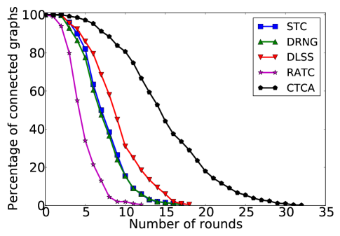
Figure 3: Lifetime comparison against different algorithms

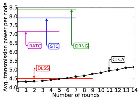
(a) The average transmission power per node plotted against time until 50% of the graphs in the simulation experiments lose connectivity.

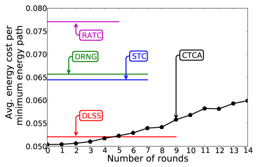
(b) The average energy consumption along the minimum energy path plotted against time until 50% of the graphs in the experiments lose connectivity.

Figure 4: A comparative performance analysis of different algorithms.

VI-B Comparative analysis against other algorithms

In this section, we compare the performance of CTCA algorithm against some of the other algorithms. Among the well-cited algorithms, our criteria for including them in this comparative analysis are the following:

• The algorithm applies to or allows application in which communication is uni-directional, where if node $N_{i}$ is within the communication radius of node $N_{j}$, node $N_{j}$ is not required to be within the communication radius of node $N_{i}$. It is the same assumption that we make in this paper.

• The communication and computational complexity for an adaptive algorithm is $O(\Delta)$ or lower each round.

Based on the above criteria, we have selected Directed Relative Neighborhood Graph (DRNG) [1], Directed Local Spanning Subgraph (DLSS) [1], Step Topology Control (STC) [2], and Routing Assisted Topology Control (RATC) [3]. In the case of the RATC algorithm, it was reported in [3] that when sensor nodes operate under a given level of 3-hop knowledge, the algorithm yields the best performance. Thus, we also allow up to 3-hop level of information to be exchanged among sensor nodes in the RATC algorithm.

In our experiments, every round, each node will send a designated data packet to every other node within the network, i.e, a node will send out $n-1$ packets each round. Data packets are routed through the minimum energy consumption path. In case of the CTCA algorithm, at the beginning of each round, each node adjusts its transmission power according to the energy situation in its local area; as for all other algorithms, each node will send out a hello message to check their neighbors’ availability.

In our simulations, we include the full energy costs of the overhead (such as hello messages) associated with executing each of the algorithms considered in the comparative analysis.

Fig.  3 reports the network lifetime achieved by the different algorithms. For each point in the graph, its x-axis value indicates the number of rounds that has passed. The y-axis value indicates the percentage of graphs (of the 200 randomly generated graphs used as a starting point in the experiments) that are still connected. As shown in the figure, a significantly larger fraction of graphs stay connected when using the CTCA compared to other previously-known algorithms. On average, we find that the life of a network is extended by more than 50% compared to other algorithms.

Fig.  4 reports the network’s parameters (the average transmission power per node and the average energy cost along the minimum energy path) achieved by the different algorithms. For static algorithms such as DLSS, DRNG, STC, and RATC, the topology of the network is determined at the very beginning of the network’s lifetime. Therefore, their network’s parameters remain the same throughout the network’s lifetime, as indicated by straight lines in Figs. 4(a) and 4(b). The CTCA algorithm, on the other hand, changes the topology of the network with time, and thus, produces different parameters each round. In Figs. 4(a) and 4(b), we have reported each algorithm’s performance until 50% of the random graphs that we have generated become disconnected. DLSS is the only algorithm that achieves average transmission power or energy cost per path comparable to the CTCA algorithm. However, as time progresses, all algorithms except CTCA retain the same average transmission power per node until the network’s functional life ends, but the CTCA algorithm adapts accordingly and preserves connectivity for much longer. It is worth noting that, in the case of the CTCA algorithm, between the first round when a graph is connected to the 14th round when it is only 50% likely that it is connected, the average transmission power per node in the CTCA algorithm increases by only about 20%. The same observation can be made for the average energy cost along the minimum energy path.

Note that, the CTCA algorithm is an algorithm that determines the topology of the network. Therefore, in our simulation, to capture how the CTCA algorithm is able to help extend the network’s functional lifetime, we only employ the simplest routing algorithm—routing the packet through the minimum energy path. The performance of the CTCA algorithm may vary depending upon the routing algorithm used to transmit data packets. An efficient routing algorithm may help extend the network’s functional lifetime even further if the energy dissipation can be distributed more evenly. However, whether or not the routing algorithm is an efficient one, the CTCA algorithm accommodates the impact of the routing algorithm because it dynamically adapts to the current energy level at each node.

VI-C Comparison against the optimal solution

In topology control algorithms, the weight of an edge usually reflects the cost of transmission through that particular link. Alternatively, if we assign the weight of an edge $(N_{i},N_{j})$ at time $t$ as:

$$w_{i,j}(t)=\frac{p(N_{i},N_{j})}{W_{i}(t)}$$ (10)

then, this weight function captures the amount of estimated lifetime consumed by the sender node $N_{i}$ if a transmission is made through link $N_{i}\rightarrow N_{j}$. A centralized topology control algorithm to minimize the maximum weight of an edge while preserving connectivity is trivial (e.g., based on removing edges from the graph in order of decreasing weight until removing an edge would destroy connectivity). Let $T_{\text{Opt},r}$ denote the maximum possible estimated lifetime of the network achieved using this optimal algorithm on the input graph in round $r$.

Let $T_{\text{CTCA},r}$ denote the estimated lifetime of the network achieved using the CTCA algorithm on the input graph in round $r$. We define the average price paid by the CTCA algorithm as:

$$\text{Average price paid}=\text{avg}\left(\frac{T_{\text{Opt},r}}{T_{\text{CTCA},r}}\right)$$

In our performance analysis, we compute the above average price paid by taking the average over multiple runs each with a different random graph as the input. We use the term price in line with the traditional terminology in game theory used in metrics comparing Nash equilibrium solutions against the social optimum (e.g., the price of anarchy [37]). In this section, we will use this metric (the average price paid by CTCA) as a measure of the quality of the solution reached by the CTCA algorithm (note that this only measures the quality of the solution and not the energy expended to reach the solution, addressed in the previous subsection in computing actual lifetimes).

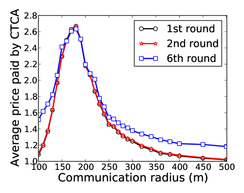
(a) The average price paid by CTCA (average ratio of the optimal lifetime and that achieved by CTCA).

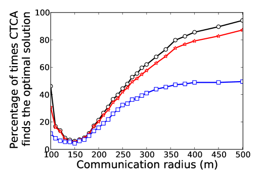
(b) The percentage of times that the CTCA algorithm finds the optimal solution.

Figure 5: The performance of the distributed CTCA algorithm in comparison to the centralized optimal algorithm in different rounds plotted against the communication radius of the nodes.

In the following set of experiments, we study the quality of the solution delivered by the distributed CTCA algorithm in comparison to the centralized optimal solution. In our experiments, we begin with sensor nodes all with the same amount of starting energy (10J) and randomly deployed in a 1000m $\times$ 1000m square region. While the energy levels of nodes at the beginning of the 1st round is the same, the uneven distribution of the energy consumption on the sensor nodes leads to unevenness in the energy levels of the nodes in subsequent rounds. Accommodating this unevenness being an important goal of this paper, we trace the performance of the CTCA algorithm in different rounds (1st, 2nd and 6th). We choose the first round because it is when energy levels are all the same. We choose the 2nd round because this is the first round at the beginning of which energy levels may be different on different nodes. We choose the 6th round because, as shown in Fig. 3, the network may have passed nearly 50% of its lifetime after this many rounds.

VI-C1 The influence of communication radius of nodes

In our first set of experiments, we study the influence of the sensor node’s maximum communication radius on the performance of the CTCA algorithm. We use 200 sensor nodes deployed in the region. We conduct 500 independent simulations and report the results in Fig. 5. Fig. 5(a) reports the average price paid by the CTCA algorithm with different values of the communication radius of nodes in each of rounds 1, 2 and 6. Fig. 5(b) reports the percentage of times that the CTCA algorithm is able to find the optimal solution for different communication radii in those same rounds.

Fig. 5(a) shows that when the communication radius is very small (e.g., at 100 meters or 10% of the length of each side in the square area), the performance of the CTCA algorithm is very close to that of the optimal algorithm (with average price paid close to 1.0). This is because, given the same sensor node density, the topology graph is already very sparse when the communication range of the nodes is relatively small. The CTCA algorithm as well as the optimal algorithm cannot do much to improve the lifetime in this situation. On the other hand, as the communication range of the sensor nodes is increased, the number of choices available to each sensor node when trying to adjust its transmission power increases. A centralized algorithm is better able to exploit these choices because of more information available to it as compared to the localized information available to each node in the distributed CTCA algorithm. As the communication range increases even more, each node is able to gain sufficient information about the region around itself even in a distributed algorithm like CTCA. Therefore, at larger communication ranges, the disparity in the performance of the distributed CTCA algorithm and the centralized optimal algorithm reduces again with the average price paid by the CTCA algorithm reaching closer to 1.0.

The above phenomenon also explains why, as shown in Fig. 5(b), the CTCA algorithm is more likely to find the optimal solution when the communication range of nodes is very low compared to when the range is intermediate. The figure also shows that, as expected, the CTCA algorithm finds the optimal solution with high likelihood when the communication range of the nodes is high. Note that the weaker performance at intermediate ranges is an inherent limitation of a distributed algorithm which works with only localized information and not necessarily of the CTCA algorithm (which performs better than other distributed algorithms as shown in the previous subsection).

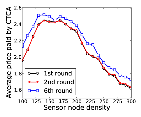
(a) The average price paid by CTCA (average ratio of the optimal lifetime and that achieved by CTCA).

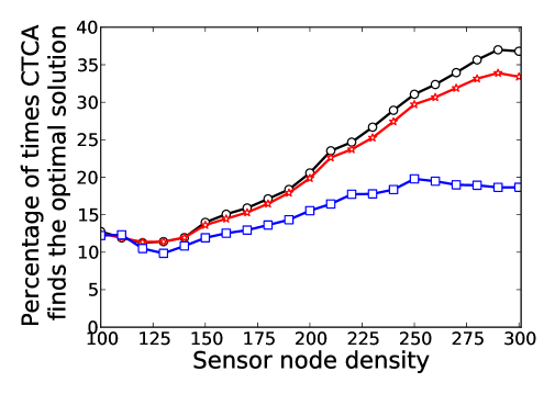
(b) The percentage of times that the CTCA algorithm finds the optimal solution.

Figure 6: The performance of the distributed CTCA algorithm in comparison to the centralized optimal algorithm in different rounds plotted against sensor node density, expressed in number of nodes per square kilometer.

It is of interest to observe that, in round 6, the disparity in the energy levels remaining on different nodes becomes larger and which, in turn, triggers more frequent cooperation between nodes and more changes in the topology. Depending on the order in which different nodes cause these changes, the potential solution space available to the CTCA algorithm can be large. As a result, even though the average performance of the CTCA algorithm in the 6th round is similar to that in other rounds, it is much less likely to reach the perfect optimal solution in the 6th round.

VI-C2 The influence of sensor node density

In our second set of experiments, we limit the maximum communication radius of each sensor node to 200 meters (when the CTCA algorithm performs close to the worst in comparison to the optimal centralized algorithm). To study the impact of the sensor node density on the performance of the CTCA algorithm, we conducted an experiment with sensor node densities ranging from 100 to 300 per square kilometer (i.e., 100 to 300 nodes in the region in our simulation experiments). The results are reported in Fig. 6. Fig. 6(a) reports the average price paid by the CTCA algorithm for different densities in different rounds. Fig. 6(b) reports the percentage of times that the CTCA algorithm is able to find the optimal solution.

In Fig. 6, we observe a similar trend as in Fig. 5 with a dip in the performance at intermediate communication ranges in the former figure and a dip in the performance at intermediate densities in the latter figure. The trend is explained by the same phenomena described earlier in the context of changes in performance with changes in the communication radius of the nodes.

VII Conclusion

In this paper, we proposed a game-theoretic approach for nodes in a sensor network to cooperatively change their transmission powers to help extend the network lifetime. We have proved the existence of a Nash equilibrium for our game and provided an algorithm, Cooperative Topology Control with Adaptation (CTCA), which achieves such an equilibrium. Our simulation results show that the CTCA algorithm is able to improve the lifetime of a wireless sensor network by more than 50% compared to the best previously-known algorithms.

To better assess the performance of the CTCA algorithm, we also compare the quality of the topology delivered by the CTCA algorithm to the optimal solution obtained using a centralized algorithm. Our results show that with increased information available to each node about its region (such as when the communication range is large), the CTCA algorithm performs closer to the optimal one. Also, the more topological options available to each node (such as when the node density is high), the more likely that the average performance of the CTCA algorithm is closer to the optimal one.

While a distributed algorithm like the CTCA is able to perform well with more information or options available at each node, we find that there is a significant gap between the average performance of the CTCA algorithm and the optimal centralized one. Even though the CTCA algorithm performs better than other distributed algorithms, this paper suggests that there may yet be more room for new research on better distributed algorithms.

While our work has used a game-theoretic approach under the constraint that the network remain connected, our algorithm can be adapted to other criteria that describe the functional life of a network (such as whether or not each portion of a certain region is covered by a sensor node within a pre-defined distance). The connectivity is captured in the term $C(\mathbf{P})$ in Equation (4) and can be replaced by a different criterion such as coverage. Our ongoing research is focused on developing and describing a generalized version of this approach.

References

- [1] N. Li and J. C. Hou, “Localized topology control algorithms for heterogeneous wireless networks,” IEEE/ACM Transactions on Networking, vol. 13, no. 6, pp. 1313–1324, December 2005.
- [2] H. Sethu and T. Gerety, “A new distributed topology control algorithm for wireless environments with non-uniform path loss and multipath propagation,” ELSEVIER Ad Hoc Networks, vol. 8, no. 3, pp. 280–294, May 2010.
- [3] R. S. Komali, A. B. MacKenzie, and P. Mahonen, “On selfishness, local information, and network optimality: A topology control example,” in Proc. International Conference on Computer Communication and Networks. New York City: IEEE, 2009, pp. 1–7.
- [4] T. S. Rappaport, Wireless Communications: Principles and Practice, 2nd ed. Upper Saddle River, NJ, USA: Prentice Hall, 2002.
- [5] S. Geng and P. Vainikainen, “Experimental investigation of the properties of multiband UWB propagation channels,” in Proc. Annual IEEE Symposium on Personal, Indoor and Mobile Radio Communications. New York City: IEEE, 2007, pp. 1–5.
- [6] Z. Sun and I. F. Akyildiz, “Channel modeling and analysis for wireless networks in underground mines and road tunnels,” IEEE Transactions on Communications, vol. 58, no. 6, pp. 1758–1768, 2010.
- [7] T. M. Chiwewe and G. P. Hancke, “A distributed topology control technique for low interference and energy efficiency in wireless sensor networks,” IEEE Transactions on Industrial Informatics, vol. 8, no. 1, pp. 11–19, 2012.
- [8] J. R. Marden, G. Arslan, and J. S. Shamma, “Cooperative control and potential games,” IEEE Transactions on Systems, Man, and Cybernetics, vol. 39, no. 6, pp. 1393 – 1407, 2009.
- [9] D. Monderer and L. S. Shapley, “Potential games,” ELSEVIER Games and economic behavior, vol. 14, no. 1, pp. 124–143, 1996.
- [10] I. Dietrich and F. Dressler, “On the lifetime of wireless sensor networks,” ACM Transactions on Sensor Networks, vol. 5, no. 1, pp. 1–39, February 2009.
- [11] J. Deng, Y. S. Han, W. B. Heinzelman, and P. K. Varshney, “Scheduling sleeping nodes in high density cluster-based sensor networks,” Springer Mobile Networks and Applications, vol. 10, no. 6, pp. 825–835, December 2005.
- [12] E. J. Duarte-Melo and M. Liu, “Analysis of energy consumption and lifetime of heterogeneous wireless sensor networks,” in Proc. IEEE Global Telecommunications Conference, vol. 1. New York City: IEEE, 2002, pp. 21–25.
- [13] L. Li and J. Y. Halpern, “Minimum energy mobile wireless networks revisited,” in Proc. IEEE International Conference on Communications. New York City: IEEE, 2001, pp. 278–283.
- [14] N. Li, J. C. Hou, and S. Lui, “Design and analysis of an MST-based topology control algorithm,” in Proc. IEEE International Conference on Computer Communications. New York City: IEEE, 2003, pp. 1702–1712.
- [15] R. Sun, J. Yuan, I. You, X. Shan, and Y. Ren, “Energy-aware weighted graph based dynamic topology control algorithm,” ELSEVIER Simulation Modelling Practice and Theory, vol. 19, no. 8, pp. 1773–1781, 2011.
- [16] M. Hajiaghayi, N. Immorlica, and V. S. Mirrokni, “Power optimization in fault-tolerant topology control algorithms for wireless multi-hop networks,” IEEE/ACM Transactions on Networking, vol. 15, no. 6, pp. 1345 – 1358, December 2007.
- [17] K. Miyao, H. Nakayama, N. Ansari, and N. Kato, “LTRT: An efficient and reliable topology control algorithm for ad-hoc networks,” IEEE Transactions on Wireless Communications, vol. 8, no. 12, pp. 6050–6058, December 2009.
- [18] P. Jianping, H. Y. Thomas, C. Lin, S. Yi, and S. S. X., “Topology control for wireless sensor networks,” in Proc. 9th annual International Conference on Mobile Computing and Networking. New York City: ACM, 2003, pp. 286–299.
- [19] R. S. Komali and A. B. MacKenzie, “Distributed topology control in ad-hoc networks: A game theoretic perspective,” in Proc. IEEE Consumer Communications and Networking Conference. New York City: IEEE, 2006, pp. 563–568.
- [20] S. Eidenbenz, V. S. A. Kumar, and S. Zust, “Equilibria in topology control games for ad hoc networks,” Springer Mobile Networks and Applications, vol. 11, no. 2, pp. 143–159, April 2006.
- [21] H. Ren and M. Q.-H. Meng, “Game-theoretic modeling of joint topology control and power scheduling for wireless heterogeneous sensor networks,” IEEE/ACM Transactions on automation science and engineering, vol. 6, no. 4, pp. 610–625, October 2009.
- [22] N. Ababneh, A. Viglas, H. Labiod, and N. Boukhatem, “ECTC: Energy efficient topology control algorithm for wireless sensor networks,” in Proc. IEEE International Symposium on a World of Wireless, Mobile and Multimedia Networks & Workshops. New York City: IEEE, 2009, pp. 1–9.
- [23] O. Younis and S. Fahmy, “Distributed clustering in ad-hoc sensor networks: A hybrid, energy-efficient approach,” in Proc. IEEE International Conference on Computer Communications. New York City: IEEE, 2004, pp. 1–12.
- [24] G. Koltsidas and F.-N. Pavlidou, “A game theoretical approach to clustering of ad-hoc and sensor networks,” Springer Telecommunication Systems, vol. 47, no. 1, pp. 81–93, 2011.
- [25] H. Üster and H. Lin, “Integrated topology control and routing in wireless sensor networks for prolonged network lifetime,” ELSEVIER Ad Hoc Networks, vol. 9, no. 5, pp. 835 – 851, 2011.
- [26] A. C. Voulkidis, M. P. Anastasopoulos, and P. G. Cottis, “Energy efficiency in wireless sensor networks: A game-theoretic approach based on coalition formation,” ACM Transactions on Sensor Networks, vol. 9, no. 4, pp. 43:1–43:27, July 2013.
- [27] W. Li, F. C. Delicato, and A. Y. Zomaya, “Adaptive energy-efficient scheduling for hierarchical wireless sensor networks,” ACM Transactions on Sensor Networks, vol. 9, no. 3, pp. 33:1–33:34, July 2013.
- [28] A. Xenakis, I. Katsavounidis, and G. Stamoulis, “Investigating wireless sensor network lifetime under static routing with unequal energy distribution,” in Proc. Asia-Pacific Signal Information Processing Association Annual Summit and Conference. New York City: IEEE, 2012, pp. 1–7.
- [29] J. Luo, A. Iyery, and C. Rosenberg, “Throughput-lifetime tradeoffs in multihop wireless networks under an SINR-based interference model,” IEEE Transactions on Mobile Computing, vol. 10, no. 3, pp. 419–433, 2011.
- [30] S. Mahfoudh and P. Minet, “Survey of energy efficient strategies in wireless ad hoc and sensor networks,” in Proc. Seventh International Conference on Networking. New York City: IEEE, 2008, pp. 1–7.
- [31] P. Santi, “Topology control in wireless ad hoc and sensor networks,” ACM Computing Surveys, vol. 37, no. 2, pp. 164–194, June 2005.
- [32] R. Machado and S. Tekinay, “A survey of game-theoretic approaches in wireless sensor networks,” ELSEVIER Computer Networks, vol. 52, no. 16, pp. 3047–3061, August 2008.
- [33] A. A. Aziz, Y. A. Sekercioglu, P. Fitzpatrick, and M. Ivanovich, “A survey on distributed topology control techniques for extending the lifetime of battery powered wireless sensor networks,” IEEE Communications Surveys Tutorials, vol. 15, no. 1, pp. 121 –144, 2013.
- [34] A. B. MacKenzie, L. DaSilva, and L. A. DaSilva, Game Theory for Wireless Engineers. San Rafael, CA, USA: Morgan and Claypool, 2006.
- [35] W. B. Heinzelman, A. P. Chandrakasan, and H. Balakrishnan, “An application-specific protocol architecture for wireless microsensor networks,” IEEE Transactions on Wireless Communications, vol. 4, pp. 660–670, October 2002.
- [36] TinyOS, “TinyOS 2.0.2 documentation,” 2008, http://tinyos.net/tinyos-2.x/doc/txt/tep113.txt.
- [37] E. Koutsoupias and C. Papadimitriou, “Worst-case equilibria,” in Proc. International Symposium on Theoretical Aspects of Computer Science. New York City: Springer, 1999, pp. 404–413.