Supplementary Document

This Supplement contains the proofs and pseudo-codes of the methods referenced in the Methodology section of the paper, as well as supplemental figures and tables for the Numerical examples section of the paper. The proofs involve the basic properties of our CTMC approach, and provide rigorous justification for the algorithms presented in the paper. The pseudo-codes illustrate the overviews of the steps of different methods used in the manuscript. The supplemental figures and tables also provide more extensive justification for the practical applicability of our method to both the phylogenetic and RNA settings.

1 Methodology

We prove here the results stated in the methodology section of the main paper.

1.1 Proposition 1

Proof.

We have, for any $x^{*}=(x_{1},x_{2},\dots,x_{n})\in{\mathcal{X}}^{*}$,

$${\mathbf{1}}(x_{n}=y) \frac{\left(\prod_{i=1}^{n-1}\nu(x_{i},x_{i+1})\right){\mathbb{P}}\left(\sum_{i=1}^{n-1}H_{i}\leq T<\sum_{i=1}^{n}H_{i}\bigg{|}X^{*}=x^{*}\right)}{{\mathbb{P}}_{x}(X_{N}=y)}$$

$$=\frac{{\mathbf{1}}(x_{n}=y){\mathbb{P}}_{x}(X_{1}=x_{1},\dots,X_{n}=x_{n})}{{\mathbb{P}}_{x}(X_{N}=y)}$$

$$\ \ \ \ \ \ \times{\mathbb{P}}\left(\sum_{i=1}^{n-1}H_{i}\leq T<\sum_{i=1}^{n}H_{i}\bigg{|}X_{1}=x_{1},\dots,X_{n}=x_{n}\right)$$

$$={\mathbf{1}}(x_{n}=y)\frac{1}{{\mathbb{P}}_{x}(X_{N}=y)}$$

$$\ \ \ \ \ \ \times{\mathbb{P}}_{x}\left(\sum_{i=1}^{n-1}H_{i}\leq T<\sum_{i=1}^{n}H_{i},X_{1}=x_{1},\dots,X_{n}=x_{n}\right)$$

$$={\mathbb{P}}_{x}(X^{*}=x^{*}|X_{N}=y).$$

Since the right hand side is a conditional distribution,

$$\pi(x^{*})={\mathbb{P}}_{x}(X^{*}=x^{*}|X_{N}=y),$$

is indeed a normalized probability mass function. ∎

1.2 Proposal distributions

We show that the proposal defined in Equation (2) of the main paper hits the target end point $y$ with probability one under the following assumptions:

1. The potential $\rho^{y}(x)$ takes the value zero if and only if $x=y$.

2. The potential always changes by one in absolute value for all proposed states:

   $$\tilde{\mathbb{P}}_{x}\left(|\rho^{y}(X_{2})-\rho^{y}(x)|=1\right)=1.$$

3. For all states $x\neq y$, there is always a way to propose a state that results in a decrease in potential:

   $$\tilde{\mathbb{P}}_{x}(\rho^{y}(X_{2})<\rho^{y}(x))>0\ \ \ \ \textrm{for all }x\in{\mathcal{X}},x\neq y.$$

To simplify the notation, we will drop the $y$ superscript for the remaining of this section.

To prove that the process always hits $y$, it is enough to show that the sequence $\rho(X_{n})$ is a supermartingale, which in our case reduces to showing that ${\mathbb{E}}[\rho(X_{2})|X_{1}]\leq\rho(X_{1}).$

Note that the last condition ensures that the normalizer $\sum_{x^{\prime}_{2}\in D(X_{1})}\nu(X_{1},x^{\prime}_{2})$ is always positive, hence our expression of the proposal is always well defined. Note that technically, we should also require ${\mathbb{P}}_{x}(\rho^{y}(X_{2})<\rho^{y}(x))>0$ to ensure that the second normalizer, $\sum_{x^{\prime}_{2}\notin D(X_{1})}\nu(X_{1},x^{\prime}_{2})$, is also positive, but if this is not the case, the proposal can always be replaced by $\nu$ in these cases without changing the conclusion of the result proven here.

Using the second condition, we have:

$${\mathbb{E}}[\rho(X_{2})|X_{1}] =\alpha_{X_{1}}(\rho(X_{1})-1)+(1-\alpha_{X_{1}})(\rho(X_{1})+1)$$

$$=1-2\alpha_{X_{1}}+\rho(X_{1})$$

$$\leq\rho(X_{1}).$$

Finally, since the supermartingale $\rho(X_{n})$ is non-negative, $\tilde{\mathbb{P}}(N<\infty)=1$, we conclude that the process always hits $y$.

1.3 Proposition 2

Let $\check{X}_{1},\check{X}_{2},\dots$ and $\check{H}_{1},\check{H}_{2},\dots$ denote the states and holding times respectively of a CTMC with rate matrix $\check{Q}$. The states take values in $\{1,2,\dots,n+1\}$, and we let $\check{\mathbb{P}}_{1}$ denote the path probabilities under this process conditioned on starting at $X_{1}=1$. Let $\check{N}$ be defined similarly to $N$ (the random number of states visited):

$$(\check{N}=n) =\left(\sum_{i=1}^{n-1}\check{H}_{i}\leq T<\sum_{i=1}^{n}\check{H}_{i}\right)$$

$$=\left\{\omega\in\check{\Omega}:\sum_{i=1}^{n-1}\check{H}_{i}(\omega)\leq T<\sum_{i=1}^{n}\check{H}_{i}(\omega)\right\}.$$

Here, $\check{\Omega}$ is an auxiliary probability space used to define the above random variables:

$$\check{X}_{i} :\check{\Omega}\to{\mathcal{X}}$$

$$\check{H}_{i} :\check{\Omega}\to[0,\infty).$$

Proof.

For all $i\in\{2,\dots,n+1\}$, only state $i-1$ has a positive rate of transitioning to state $i$, therefore $(\check{X}_{i}=j)\subset(\check{X}_{i-1}=j-1)$ for all $j$. Applying this inductively yields:

$$\left(\exp(T\check{Q})\right)_{1,n} =\check{\mathbb{P}}_{1}\left(\check{X}_{\check{N}}=n\right)$$

$$=\check{\mathbb{P}}_{1}\left(\check{X}_{\check{N}}=n,\check{X}_{\check{N}-1}=n-1\right)$$

$$\ \ \vdots$$

$$=\check{\mathbb{P}}_{1}\left(\check{X}_{\check{N}}=n,\check{X}_{\check{N}-1}=n-1,\dots,\check{X}_{1}=n-\check{N}+1\right)$$

$$=\check{\mathbb{P}}_{1}\left(\check{N}=n,\check{X}_{1}=1,\check{X}_{2}=2,\dots,\check{X}_{n}=n\right)$$

$$=\check{\mathbb{P}}_{1}\left(\check{N}=n\right)\check{\mathbb{P}}_{1}\left(\check{X}_{1}=1,\check{X}_{2}=2,\dots,\check{X}_{n}=n|\check{N}=n\right)$$

$$=\check{\mathbb{P}}_{1}\left(\check{N}=n\right)\prod_{i=2}^{n}\check{\mathbb{P}}(\check{X}_{i}=i|\check{X}_{i-1}=i-1)$$

$$=\check{\mathbb{P}}_{1}\left(\check{N}=n\right)$$

$$=\int\int\cdots\int_{h_{i}>0:h_{1}+h_{2}+\cdots+h_{n}=T}g(h_{1},h_{2},\dots,h_{n})\,\mathrm{d}h_{1}\,\mathrm{d}h_{2}\dots\,\mathrm{d}h_{n}.$$

∎

In this part, for further clarity, we give the pseudo-codes of the proposed algorithms.

Our novel method (denoted as Time Integrated Path Sampling, TIPS) is demonstrated in Algorithm 1. This method uses the propose method introduced in Algorithm 2 in order to sample each particle, consisting of a sequence of states starting at $x$ and ending at the target, $y$. The propose method also employs Algorithm 3 as a part of its structure to sample the particles hitting the target.

Algorithm 1 : TIPS($x,y,T$)

  $s\leftarrow 0$

  for $k=1,2,\dots,K$ do

     $(L,\tilde{p},p)\leftarrow$ propose$(x,\{y\})$

     $\check{Q}\leftarrow\check{Q}(L)$ {See Section ‘Analytic jump integration’}

     $n=|L|$ {The length of the list of states $L$}

     $s\leftarrow s+p\times(\exp(T\check{Q}))_{1,n}/\tilde{p}$

  end for

  return  $s/K$

Algorithm 2 : propose($x,A$)

  $(L,\tilde{p},p)\leftarrow$proposeHittingPath($x,A,$ false)

  $n\sim$ Geo$(\cdot,\beta)$ {Geometric with support 1, 2, …}

  $\tilde{p}\leftarrow p\ \times$ Geo$(n;\beta)$ {Multiply by geometric probability mass function}

  for $i=2,3,\dots,n$ do

     $x^{\prime}\leftarrow$ last$(L)$ {Last state visited in the list $L$}

     $(L^{\prime},\tilde{p}^{\prime},p^{\prime})\leftarrow$proposeHittingPath($x^{\prime},A,$ true)

     $\tilde{p}\leftarrow\tilde{p}\times\tilde{p}^{\prime}$

     $p\leftarrow p\times p^{\prime}$

     $L\leftarrow L\circ L^{\prime}$ {Concatenation of the two lists}

  end for

  return  $(L,\tilde{p},p)$

Algorithm 3 : proposeHittingPath($x,A,b$)

  $p\leftarrow 1$

  $\tilde{p}\leftarrow 1$

  $L\leftarrow$ list($x$) {Creates a new list containing the point $x$}

  for $i=1,2,\dots$ do

     if $x\in A$ and (not($b$) or $i>1$) then

        return  $(L,\tilde{p},p)$

     end if

     $x^{\prime}|x\sim\tilde{\mathbb{P}}(\cdot|X_{i-1}=x)$

     $\tilde{p}\leftarrow\tilde{p}\times\tilde{\mathbb{P}}(X_{i}=x^{\prime}|X_{i-1}=x)$

     $p\leftarrow p\times\nu(x,x^{\prime})$

     $L\leftarrow L\circ x^{\prime}$

     $x\leftarrow x^{\prime}$

  end for

An overview of the parameter estimation method explained in the manuscript is also shown in Algorithm 4. In this algorithm, statio() computes the stationary probability mass function, for example Poisson in the Poisson Indel Process example Bouchard-Côté & Jordan (2012).

Algorithm 4 : TIPS-parameters($\{x_{i},y_{i},T_{i}\}$)

  Initialization:

  Choose initial parameter $\theta^{(1)}$

  $z\leftarrow 0$

  for $(t=2,\cdots,T)$ do

     $\theta^{*}\sim q(\cdot|\theta^{(t-1)})$

     $z^{*}\leftarrow 1$

     for all data index $i$ do

        $z^{*}\leftarrow z^{*}\times$ TIPS($x_{i},y_{i},T_{i}$) $\times$ statio($x_{i}$)

     end for

     $r\leftarrow\frac{p(\theta^{*})}{p(\theta^{(t-1)})}\ \frac{z^{*}}{z}\ \frac{q(\theta^{(t-1)}|\theta^{*})}{q(\theta^{*}|\theta^{(t-1)})}$

     Sample $u\sim\textrm{Uniform}(0,1)$

     if $u<\min\{1,r\}$ then

        $z\leftarrow z^{*}$

        $\theta^{(t)}\leftarrow\theta^{*}$

     else

        $\theta^{(t)}\leftarrow\theta^{(t-1)}$

     end if

  end for

Moreover, Algorithm 5, extends Saeedi & Bouchard-Côté (2011) and demonstrate the revised sequential Monte Carlo (SMC) method for approaching more general types of observations, for example a series of partially observed states, or a phylogenetic tree with observed leaves. Note that this algorithm is amenable to parallelization Lee et al. (2010); Jun et al. (2012).

Algorithm 5 : TIPS-SMC($A_{i},T_{i})$

  Initialization:

  $w_{0,k}\leftarrow 1/K$

  $x_{0,k}\leftarrow$ nil

  for $g=1,2,\dots,G$ do

     for $k=1,2,\dots,K$ do

        $(L,\tilde{p},p)\leftarrow$ propose$(x_{g-1,k},A_{g})$

        $\check{Q}\leftarrow\check{Q}(L)$ {See Section ‘Analytic jump integration’}

        $n=|L|$ {The length of the list of states $L$}

        $w_{g,k}\leftarrow w_{g-1,k}\times p\times(\exp(T_{g}\check{Q}))_{1,n}/\tilde{p}$

        $x_{g,k}\leftarrow$ last$(L)$

     end for

     if ESS$(w_{g,\cdot})<$ threshold then

        $(w_{g,\cdot},x_{g,\cdot})\leftarrow$ resample$(w_{g,\cdot},x_{g,\cdot})$ {Perform SMC resampling step}

     end if

  end for

2 Numerical examples

In this section we have figures and tables for both the phylogenetic and RNA settings. These give more detail on the results that we have obtained from applying our method to these CTMCs.

2.1 Phylogenetics

2.1.1 Validation

We generated 200 pair-wise alignments with $T=3/10,\lambda=\lambda_{\textrm{pt}}=2,\mu=\mu_{\textrm{pt}}=1/2$ and held out the mutations and the true value of parameters $\lambda$ and $\mu$. We approximate the posterior using our method. We show the results of $\lambda$ in the paper and $\mu$ in Figure 1. In both cases the posterior approximation is shown to closely mirror the numerical approximation. The evolution of the Monte Carlo quartiles computed on the prefixes of Monte Carlo samples also show that the convergence is rapid in this case.

Exact	TIPS-parameters	Samples	Monte Carlo Quartiles

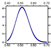
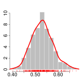
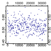
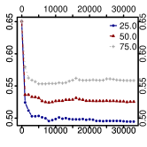
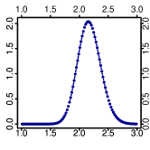
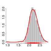
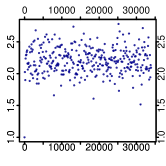
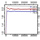
Figure 1: Results of parameter $\mu$ ($1^{st}$ row) in the validation of the implementation using the Poisson Indel Process (PIP). From left to right: posterior obtained via numerical methods; approximate posterior using our method with 64 particles and 35,000 GIMH iterations; sampled parameter values; convergence of the quantile computed from the GIMH output. For further clarity, the results of parameter $\lambda$ ($2^{nd}$ row) are also shown.

		ESS
Parameter	N. Particles	FS	TIPS
$\lambda$	10	175.9	1,556.2
	100	44.6	7,082.7
	1000	25.6	927.8
	10000	35.2	147.5
	100000	12.2	12.4
$\mu$	10	11.3	774.1
	100	90.2	6,761.2
	1000	31.0	903.5
	10000	48.3	128.9
	100000	16.7	12.0

Table 1: Varying the number of particles per MCMC step. We show the effective sample size obtained in a fixed computational budget (wall clock time of 3 days), comparing a GIMH based on our method (TIPS), compared to the forward sampling method (FS). Refer to Section 3 of the main paper for details.

2.1.2 Tree inference

We start by introducing some notation for data on a phylogenetic tree $\tau$. Let $v_{0}$ denote the root, and $V(\tau)$ the other nodes. Let $\varrho(v)$ denote the parent of the node $v\in V(\tau)$. Let $X^{*(v)}=(X^{(v)}_{1},\cdots,X^{(v)}_{N_{v}})$ denote the sequence of molecular strings that evolve from $\varrho(v)$ to $v$. The string $X^{(v)}_{N_{v}}$ at Node $v$ is also denoted by $X^{(v)}$ for simplicity. Note that only the strings at the leaves are observed, denoted ${\mathcal{Y}}$. Denote all unobserved strings by $X^{*}(\tau)=\{X^{*(v)}:v\in V(\tau)\}\backslash{\mathcal{Y}}$, where $\backslash$ is the set difference symbol. The probability of ${\mathcal{Y}}$ and $X^{*}(\tau)=x^{*}(\tau)$ given $\tau,\theta$ is

$${\mathbb{P}}_{\theta}\bigg{(}{\mathcal{Y}},X^{*}(\tau)=x^{*}(\tau)\bigg{|}\tau\bigg{)}=$$

$${\mathbb{P}}\left(X^{*(v_{0})}=x^{*(v_{0})}\right)\prod_{v\in V(\tau)}{\mathbb{P}}_{x^{(\varrho(v))},\theta}\left(X^{*(v)}=x^{*(v)}\right).$$

We use an improper uniform distribution over the strings as the distribution for the root sequence.

In the Bayesian framework, we aim at the posterior on $\tau$, $X^{*}(\tau)$, $\theta$ given ${\mathcal{Y}}$, which has a density proportional to $\gamma(\tau,x^{*}(\tau),\theta)={\mathbb{P}}_{\theta}({\mathcal{Y}},X^{*}(\tau)=x^{*}(\tau)|\tau)p(\tau)p(\theta)$, where $p(\tau)$ is a prior for $\tau$.

For fixed evolutionary parameters, we use the framework of Wang (2012) to estimate the posterior of $\tau$. In this framework, we let the $r$-th partial state $s_{r}$ be a forest that includes the forest topology and the associated branch lengths, denoted $\tau_{r}$, as well as the unobserved strings at the root of each tree in that forest, $x^{*}(\tau_{r})$; i.e. $s_{r}=(\tau_{r},x^{*}(\tau_{r}))$. We used the following sequence of intermediate distributions over forests: $\gamma(s_{r})=\prod_{\tau_{i}\in s_{r}}\gamma(\tau_{i},x^{*}(\tau_{i}))).$ In the weight update step, besides proposing two branch lengths and randomly choosing a pair of trees from the current forest to merge (as in Wang (2012)), we use the proposal distribution described in the Methodology Section of the main paper for proposing the hidden strings, with the only difference that a root sequence is selected uniformly among the intermediate strings on the proposed path. Algorithm 6 shows the component of the algorithm not present in previous work: proposing a root sequence and two discrete paths $L_{\textrm{left}}$ and $L_{\textrm{right}}$ linking this root to its two children. We assume that the pair of sequences to merge, $x_{\textrm{left}}$ and $x_{\textrm{right}}$, as well as the branch lengths connecting each to the newly formed root, $T_{\textrm{left}},T_{\textrm{right}}$, have been picked by a standard phylogenetic SMC proposal, with proposal density $\tilde{p}_{\textrm{tree}}$. These become inputs to Algorithm 6, which returns $(L_{\textrm{left}},L_{\textrm{right}},\tilde{p},p)$. From this output, we compute two auxiliary rate matrices, $\check{Q}_{\textrm{left}}=\check{Q}(L_{\textrm{left}})$ and $\check{Q}_{\textrm{right}}=\check{Q}(L_{\textrm{right}})$, one for each newly formed branch, using the same method as before.

Given all this information, we update the particle weights as follows:

$$w_{g,k}=w_{g-1,k}\frac{p\ \textrm{statio}(x_{\textrm{left}})}{\tilde{p}\ \tilde{p}_{\textrm{tree}}}\ (\exp(T_{\textrm{left}}\check{Q}_{\textrm{left}}))_{1,|L_{\textrm{left}}|}\ (\exp(T_{\textrm{right}}\check{Q}_{\textrm{right}}))_{1,|L_{\textrm{right}}|}.$$

Algorithm 6 : phylo-sequence-proposal($x_{\textrm{left}},T_{\textrm{left}},x_{\textrm{right}},T_{\textrm{right}}$)

  $(L,\tilde{p},p)\leftarrow$ propose($x_{\textrm{left}},x_{\textrm{right}},T_{\textrm{left}}+T_{\textrm{right}}$)

  $i\sim$ Unif$\{1,2,\dots,|L|\}$

  $\tilde{p}\leftarrow\tilde{p}\times 1/|L|$

  $L_{\textrm{left}}\leftarrow$ reverse(sublist($L,1,i$))

  $L_{\textrm{right}}\leftarrow$ sublist($L,i,|L|$)

  return  $(L_{\textrm{left}},L_{\textrm{right}},\tilde{p},p)$

We simulated subsets of molecular sequences with different random seeds according to our evolutionary model. The parameters are: SSM length=3, $\theta_{sub}=0.03$, $\lambda_{pt}=0.05$, $\mu_{pt}=0.2$, $\lambda_{SSM}=2.0$, and $\mu_{SSM}=2.0$. A subset of the data is shown in the Figure 2.

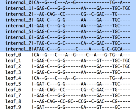
Figure 2: Sequence Simulation. One subset of simulated sequence data for the experiments on trees via SMC.

2.2 RNA Folding Pathways

To compare our method (denoted as TIPS) to that of forward sampling (denoted as FS), we first obtained an absolute accuracy by computing the matrix exponential. Then we computed the absolute log error estimate $\hat{p}$ (i.e., error($\hat{p}$) $=|\log\hat{p}-\log{\mathbb{P}}_{x}(X_{N}=y)|$) of our method and forward sampling on the RNA molecules shown in Table 2. These RNA sequences are short, due to the limit in the size of matrix computed using the matrix exponential. The state spaces for the first two RNA sequences were sufficiently small for computation of the matrix exponential. The complete state space of the last two RNAs were too large for the matrix exponential, so we sampled a subset of the state space.

Sequence	Length	$|{\mathcal{X}}|$	$|S|$
1AFX	12	70	-
1XV6	12	48	-
RNA21	21	$\sim{1100}$	657
HIV	23	$\sim{1500}$	266

Table 2: Biological RNA Sequences.

Figures 3a, 3d show the performance of the FS and TIPS methods, for two short molecules 1AFX and 1XV6, on selective folding times, $\{0.5,2,8\}$. Figures 3b, 3e show the CPU times (in milliseconds) corresponding to the minimum number of particles required to satisfy the certain accuracy level, $I=$ {$\hat{p}:$ error($\hat{p}$) $<1.0$} on different folding times including the selective ones.

The variances of FS and TIPS weights, for $5^{6}=15625$ particles, are also computed and compared on different folding times (see Figures 3c, 3f).

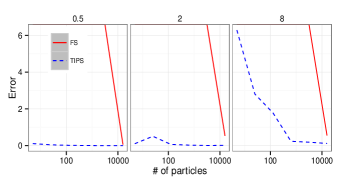
(a) 1AFX- error

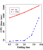
(b) 1AFX- CPU time (ms)

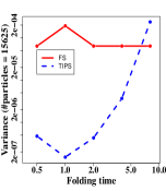
(c) 1AFX- variance

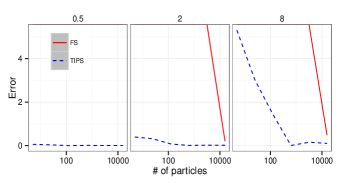
(d) 1XV6 - error

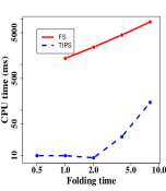
(e) 1XV6 - CPU time (ms)

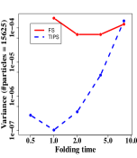
(f) 1XV6 - variance

Figure 3: Performance of our method (TIPS) and forward sampling (FS) on 1AFX and 1XV6 molecules with their whole state space. The relative errors of the estimates vs. folding times, {0.5,2,8} are shown (left) along with the CPU times corresponding to the minimum number of particles required to satisfy the accuracy level $I$ in milliseconds (middle) and the variance of TIPS and FS estimations (right) on folding times, $\{0.5,1,\cdots,8\}$.

Our method has two main tuning parameters, a geometric parameter, $\beta$, over the number of repeated excursions from $y$ to itself, and a parameter, $\alpha$, weighting the probability of the steps decreasing the value of the potential. We found that the accuracy of the sampler in the case of RNA folding pathways was sensitive to the setting of the parameters (see Figure 4). Parameter tuning is an important area of future work.

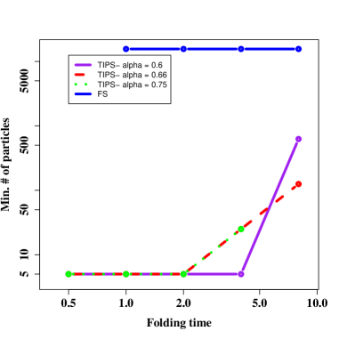
(a)

Figure 4: Tuning parameter $\alpha$. Performance of our method (TIPS) using different values of $\alpha$ compared to forward sampling (FS) for estimating the folding pathway of the 1XV6 molecule on its whole state space.

(a)

(b)

(c)

(d)

(e)

(f)

(g)

(h)

(i)

Figure 5: An example of a sampled folding pathway for the HIV23 molecule with $T=0.125$.

References

• Akkouchi (2008) Akkouchi, M. . On the convolution of exponential distributions. Journal of the Chungcheong Mathematical Society, 21(4):502–510, 2008.
• Amari & Misra (1997) Amari, S. and Misra, R. . Closed-form expressions for distribution of sum of exponential random variables. IEEE Transactions on Reliability, 46(4):519–522, 1997.
• Andrieu & Roberts (2009) Andrieu, C. and Roberts, G. O. . The pseudo-marginal approach for efficient Monte Carlo computations. The Annals of Statistics, 37(2):697–725, 2009.
• Andrieu et al. (2010) Andrieu, C. , Doucet, A. , and Holenstein, R. . Particle Markov chain Monte Carlo methods. J. R. Statist. Soc. B, 72(3):269–342, 2010.
• Arribas-Gil & Matias (2012) Arribas-Gil, A. and Matias, C. . A context dependent pair hidden Markov model for statistical alignment. Statistical Applications in Genetics and Molecular Biology, 11(1):1–29, 2012.
• Beaumont (2003) Beaumont, M. A. . Estimation of population growth or decline in genetically monitored populations. Genetics, 164(3):1139–1160, 2003.
• Bouchard-Côté & Jordan (2012) Bouchard-Côté, A. and Jordan, M. I. . Evolutionary inference via the Poisson indel process. Proc. Natl. Acad. Sci., 10.1073/pnas.1220450110, 2012.
• Bouchard-Côté et al. (2012) Bouchard-Côté, A. , Sankararaman, S. , and Jordan, M. I. . Phylogenetic inference via sequential Monte Carlo. Syst. Biol., 61:579–593, 2012.
• Fan & Shelton (2008) Fan, Y. and Shelton, C. . Sampling for approximate inference in continuous time Bayesian networks. In Tenth International Symposium on Artificial Intelligence and Mathematics, 2008.
• Felsenstein (1981) Felsenstein, J. . Evolutionary trees from DNA sequences: a maximum likelihood approach. J. Mol. Evol., 17:368–376, 1981.
• Felsenstein (2003) Felsenstein, J. . Inferring phylogenies. Sinauer Associates, 2003.
• Flamm et al. (2000) Flamm, C. , Fontana, W. , Hofacker, I. , and Schuster, P. . RNA folding at elementary step resolution. RNA, 6:325–338, 2000.
• Grassmann (1977) Grassmann, W. K. . Transient solutions in Markovian queueing systems. Computers and Operations Research, 4:47–100, 1977.
• Hickey & Blanchette (2011) Hickey, G. and Blanchette, M. . A probabilistic model for sequence alignment with context-sensitive indels. Journal of Computational Biology, 18(11):1449–1464, 2011. doi: doi:10.1089/cmb.2011.0157.
• Huelsenbeck & Ronquist (2001) Huelsenbeck, J. P. and Ronquist, F. . MRBAYES: Bayesian inference of phylogenetic trees. Bioinformatics, 17(8):754–755, 2001.
• Hutter et al. (2009) Hutter, F. , Hoos, H. H. , Leyton-Brown, K. , and Stützle, T. . ParamILS: an automatic algorithm configuration framework. Journal of Artificial Intelligence Research, 36:267–306, October 2009.
• Jun et al. (2012) Jun, S.-H. , Wang, L. , and Bouchard-Côté, A. . Entangled Monte Carlo, 2012.
• Juneja & Shahabuddin (2006) Juneja, S. and Shahabuddin, P. . Handbooks in Operations Research and Management Science, volume 13, chapter Rare-Event Simulation Techniques: An Introduction and Recent Advances, pp.  291–350. Elsevier, 2006.
• Kirkpatrick et al. (2013) Kirkpatrick, B. , Hajiaghayi, M. , and Condon, A. . A new model for approximating RNA folding trajectories and population kinetics. Computational Science & Discovery, 6, January 2013.
• Lakner et al. (2008) Lakner, C. , van der Mark, P. , Huelsenbeck, J. P. , Larget, B. , and Ronquist, F. . Efficiency of Markov chain Monte Carlo tree proposals in Bayesian phylogenetics. Syst. Biol., 57(1):86–103, 2008.
• Lee et al. (2010) Lee, A. , Yau, C. , Giles, M. B. , Doucet, A. , and Holmes, C. C. . On the utility of graphics cards to perform massively parallel simulation of advanced Monte Carlo methods. Journal of Computational and Graphical Statistics, 19(4):769–789, 2010.
• Morrison (2009) Morrison, D. A. . Why would phylogeneticists ignore computerized sequence alignment? Syst. Biol., 58(1):150–158, 2009.
• Munsky & Khammash (2006) Munsky, B. and Khammash, M. . The finite state projection algorithm for the solution of the chemical master equation. J. Chem. Phys., 124(4):044104–1 – 044104–13, 2006.
• Rao & Teh (2011) Rao, V. and Teh, Y. W. . Fast MCMC sampling for Markov jump processes and continuous time Bayesian networks. In Proceedings of the Twenty-Seventh Conference Annual Conference on Uncertainty in Artificial Intelligence (UAI-11), pp. 619–626, Corvallis, Oregon, 2011. AUAI Press.
• Rao & Teh (2012) Rao, V. and Teh, Y. W. . MCMC for continuous-time discrete-state systems. NIPS, 2012.
• Saeedi & Bouchard-Côté (2011) Saeedi, A. and Bouchard-Côté, A. . Priors over Recurrent Continuous Time Processes. NIPS, 24:2052–2060, 2011.
• Schaeffer (2012) Schaeffer, J. M. . The multistrand simulator: Stochastic simulation of the kinetics of multiple interacting dna strands. Master’s thesis, California Institute of Technology, 2012.
• Teh et al. (2008) Teh, Y. W. , Daumé III, H. , and Roy, D. M. . Bayesian agglomerative clustering with coalescents. In Advances in Neural Information Processing Systems (NIPS), 2008.
• Venkataraman et al. (2010) Venkataraman, S. , Dirks, R. M. , Ueda, C. T. , and Pierce, N. A. . Selective cell death mediated by small conditional RNAs. Proc. Natl. Acad. Sci., 107(39):16777–16782, 2010. doi: 10.1073/pnas.1006377107. URL http://www.pnas.org/content/107/39/16777.abstract.
• Wang (2012) Wang, L. . Bayesian Phylogenetic Inference via Monte Carlo Methods. PhD thesis, The University Of British Columbia, August 2012.
• Wang et al. (2013) Wang, Z. , Mohamed, S. , and de Freitas, N. . Adaptive Hamiltonian and Riemann Monte Carlo samplers. In International Conference on Machine Learning (ICML), 2013.