SO(10) Yukawa Unification after the First Run of the LHC

Abstract

In this talk we discuss SO(10) Yukawa unification and its ramifications for phenomenology. The initial constraints come from fitting the top, bottom and tau masses, requiring large $\tan\beta\sim 50$ and particular values for soft SUSY breaking parameters. We perform a global $\chi^{2}$ analysis, fitting the recently observed ‘Higgs’ with mass of order 125 GeV in addition to fermion masses and mixing angles and several flavor violating observables. We discuss two distinct GUT scale boundary conditions for soft SUSY breaking masses. In both cases we have a universal cubic scalar parameter, $A_{0}$. In the first case we consider universal gaugino masses, and universal scalar masses, $m_{16}$, for squarks and sleptons; while in the latter case we have non-universal gaugino masses and either universal scalar masses, $m_{16}$, for squarks and sleptons or D-term splitting of scalar masses. We discuss the spectrum of SUSY particle masses and consequences for the LHC.

1 Introduction

Fermion masses and mixing angles are manifestly hierarchical. The simplest way to describe this hierarchy is with Yukawa matrices which are also hierarchical. Moreover the most natural way to obtain the hierarchy is in terms of effective higher dimension operators of the form

$$W\supset 16_{3}\ 10\ 16_{3}+16_{3}\ 10\ \frac{45}{M}\ 16_{2}+\cdots.$$ (1)

This version of SO(10) models has the nice features that it only requires small representations of SO(10), has many predictions and can, in principle, find an UV completion in string theory. There are a long list of papers by authors such as Albright, Anderson, Babu, Barr, Barbieri, Berezhiani, Blazek, Carena, Chang, Dermisek, Dimopoulos, Hall, Masiero, Murayama, Pati, Raby, Romanino, Rossi, Starkman, Wagner, Wilczek, Wiesenfeldt, and Willenbrock which have followed this line of model building.

The only renormalizable term in $W$ is $\lambda\ 16_{3}\ 10\ 16_{3}$ which gives Yukawa coupling unification

$$\lambda=\lambda_{t}=\lambda_{b}=\lambda_{\tau}=\lambda_{\nu_{\tau}}$$ (2)

at $M_{GUT}$. Note, one CANNOT predict the top mass due to large SUSY threshold corrections to the bottom and tau masses, as shown in Hall et al. (1994); Carena et al. (1994); Blazek et al. (1995). These corrections are of the form

$$\delta m_{b}/m_{b}\propto\frac{\alpha_{3}\ \mu\ M_{\tilde{g}}\ \tan\beta}{m_{\tilde{b}}^{2}}+\frac{\lambda_{t}^{2}\ \mu\ A_{t}\ \tan\beta}{m_{\tilde{t}}^{2}}+{\rm log\ corrections}.$$ (3)

So instead we use Yukawa unification to predict the soft SUSY breaking masses!! In order to fit the data, we need

$$\delta m_{b}/m_{b}\sim-2\%.$$ (4)

For a short list of references on this subject, see Blazek et al. (2002a, b); Baer and Ferrandis (2001); Auto et al. (2003); Tobe and Wells (2003); Dermisek et al. (2003, 2005); Baer et al. (2008a, b, 2009a); Badziak et al. (2011); Gogoladze et al. (2012); Anandakrishnan et al. (2012); Anandakrishnan and Raby (2013); Anandakrishnan et al. (2013).

2 Gauge and Yukawa Unification with Universal Gaugino Masses

In the first case we take $\mu\ M_{\tilde{g}}>0$, thus we need $\mu\ A_{t}<0$ Anandakrishnan et al. (2012, 2013). We assume the following minimal set of GUT scale boundary conditions – universal squark and slepton masses, $m_{16}$, universal cubic scalar parameter, $A_{0}$, universal gaugino masses, $M_{1/2}$, and non-universal Higgs masses [NUHM] or ‘just so’ Higgs splitting, $m_{H_{u}},\ m_{H_{d}}$ or $m_{H_{u(d)}}^{2}=m_{10}^{2}[1-(+)\Delta_{m_{H}}^{2}]$. We then perform a global $\chi^{2}$ analysis fitting the 11 observables as a function of the 11 arbitrary parameters, Fig. 1.

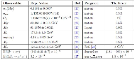
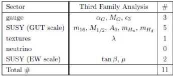
Figure 1: (Left) The 11 low energy observables which enter the $\chi^{2}$ function. (Right) The 11 arbitrary parameters which are varied to minimize $\chi^{2}$.

We find that fitting the top, bottom and tau mass forces us into the region of SUSY breaking parameter space with

$$A_{0}\approx-2m_{16},\;\;m_{10}\approx\sqrt{2}\ m_{16},\;\;m_{16}>\ {\rm few\ TeV},\;\;\mu,M_{1/2}\ll m_{16};$$ (5)

and, finally,

$$\tan\beta\approx 50.$$ (6)

In addition, radiative electroweak symmetry breaking requires $\Delta_{m_{H}}^{2}\approx 13\%$, with roughly half of this coming naturally from the renormalization group running of neutrino Yukawa couplings from $M_{G}$ to $M_{N_{\tau}}\sim 10^{13}$ GeV Blazek et al. (2002a, b).

It is very interesting that the above region in SUSY parameter space results in an inverted scalar mass hierarchy at the weak scale with the third family scalars significantly lighter than the first two families Bagger et al. (2000). This has the nice property of suppressing flavor changing neutral current and CP violating processes.

2.1 Heavy squarks and sleptons

Considering the theoretical and experimental results for the branching ratio $BR(B\rightarrow X_{s}\gamma)$, we argue that $m_{16}\geq 8$ TeV. The experimental value $BR(B\rightarrow X_{s}\gamma)_{\rm exp}=(3.55\pm 0.26)\times 10^{-4}$, while the NNLO Standard Model theoretical value is $BR(B\rightarrow X_{s}\gamma)_{\rm th}=(3.15\pm 0.23)\times 10^{-4}$. The amplitude for the process $B\rightarrow X_{s}\gamma$ is proportional to the Wilson coefficient, $C_{7}$. $C_{7}=C_{7}^{SM}+C_{7}^{SUSY}$ and, in order to fit the data, we see that $C_{7}\approx\pm C_{7}^{SM}$. Thus $C_{7}^{SUSY}\approx-2C_{7}^{SM}\;{\rm or}\;C_{7}^{SUSY}\approx 0$. The dominant SUSY contribution to the branching ratio comes from a stop - chargino loop with $C_{7}^{SUSY}\sim C_{7}^{\chi^{+}}\sim\frac{\mu\ A_{t}}{\tilde{m}^{2}}\ \tan\beta\times sign(C_{7}^{SM})$ (see Fig. 2). Hence, in the former case (which allows for light scalars) $C_{7}\approx-C_{7}^{SM}$, while in the latter case (with heavy scalars) $C_{7}\approx C_{7}^{SM}$.

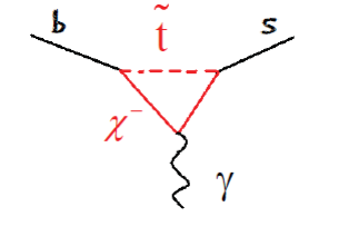
Figure 2: Dominant contribution to the process $b\rightarrow s\ \gamma$ in the MSSM.

Recent LHCb data on the $BR(B\rightarrow K^{*}\ \mu^{+}\ \mu^{-})$ now favors $C_{7}\approx+C_{7}^{SM}$ Aaij et al. (2013) (see Fig. 3).

Figure 3: The forward-backward asymmetry for the process $B\rightarrow K^{*}\ \mu^{+}\ \mu^{-}$ measured by LHCb.

This tension between the processes $b\rightarrow s\gamma$ and $b\rightarrow s\ \ell^{+}\ \ell^{-}$ was already discussed by Albrecht et al. Albrecht et al. (2007). In order to be consistent with this data one requires $C_{7}^{\chi^{+}}\approx 0$ or $C_{7}\approx C_{7}^{SM}+C_{7}^{SUSY}\approx+C_{7}^{SM}$ and therefore $m_{16}\geq 8$ TeV.

In 2007, Albrecht et al. Albrecht et al. (2007) performed a global $\chi^{2}$ analysis of this theory (including the Yukawa structure for all three families). Two of the tables from their paper are exhibited in Fig. 4. This analysis included 27 low energy observables and a reasonable fit to the data was only found for $m_{16}=10$ TeV. Note, the Higgs mass was predicted to be 129 GeV.

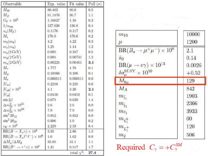
Figure 4: The results obtained by Albrecht et al. for $m_{16}=10$ TeV.

2.2 Light Higgs mass

An approximate formula for the light Higgs mass is given by Carena et al. (1996)

$$m_{h}^{2}\approx M_{Z}^{2}\ \cos^{2}2\beta+\frac{3g^{2}m_{t}^{4}}{8\pi^{2}m_{W}^{2}}\left[\ln\left(\frac{M_{SUSY}^{2}}{m_{t}^{2}}\right)+\frac{X_{t}^{2}}{M_{SUSY}^{2}}\left(1-\frac{X_{t}^{2}}{12M_{SUSY}^{2}}\right)\right]$$ (7)

where $X_{t}=A_{t}-\mu/\tan\beta$. The light Higgs mass is maximized as a function of $X_{t}$ for $X_{t}/M_{SUSY}=\pm\sqrt{6}$, referred to as maximal mixing. Hence we see that for large values of $A_{t}$ and $M_{SUSY}$ it is quite easy to obtain a light Higgs mass of order 125 GeV.

2.3 $B_{s}\rightarrow\mu^{+}\ \mu^{-}$

In this section we argue that the light Higgs boson must be Standard Model-like. To do this we show that the CP odd Higgs boson, $A$, must have mass greater than $\sim$ 1 TeV and as a consequence this is also true for the CP even Higgs boson, $H$, and the charged Higgs bosons, $H^{\pm}$, as well. This is the well-known decoupling limit in which the light Higgs boson couples to matter just like the Standard Model Higgs.

Consider the branching ratio $BR(B_{s}\rightarrow\mu^{+}\ \mu^{-})$ which in the Standard Model is $\sim 3\times 10^{-9}$. In the MSSM this receives a contribution proportional to $\sim\frac{\tan\beta^{6}}{m_{A}^{4}}$. Recent experimental results give Aaij et al. (2012)

$$LHCb\;: =(3.2\stackrel{{\scriptstyle+1.5}}{{-1.2}}\pm 0.2)\times 10^{-9}\; {\rm with}\;1\ {\rm fb}^{-1}(7\;{\rm TeV})\;{\rm and}\;1.1\ {\rm fb}^{-1}(8\;{\rm TeV}).$$ (8)

Since we have $\tan\beta\sim 50$, our only choice is to take the CP odd Higgs mass to be large with $m_{A}\geq 1$ TeV. This is the decoupling limit; hence the light Higgs is SM-like.

2.4 Gluino Mass

We find an upper bound on the gluino mass (constrained by fitting both the bottom quark and light Higgs masses). For $m_{16}=20$ TeV the upper bound at 90% CL is $m_{\tilde{g}}\lesssim 2$ TeV (see Fig. 5). For $m_{16}=30$ TeV the upper bound at 90% CL increases to $m_{\tilde{g}}\lesssim 2.8$ TeV. Note, a gluino with mass $m_{\tilde{g}}\lesssim 1.9$ TeV should be discovered at LHC 14 with 300 fb^-1 of data at 5 $\sigma$ 1244669 (2013)!

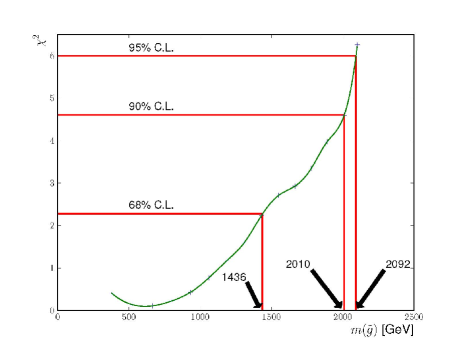
Figure 5: $\chi^{2}$ as a function of the gluino mass obtained by varying $M_{1/2}$ for fixed $m_{16}=20$ TeV or 2 degrees of freedom.

The gluinos in our model prefer to be light, so an important question is what are the present LHC bounds on gluinos in our model? Consider one benchmark point with the spectrum, Tables 6.

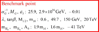
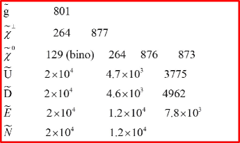
Figure 6: (Left) The value of the 11 parameters determining the benchmark point. (Right) The SUSY particle spectrum for this benchmark point.

The gluino decay branching fractions for this benchmark point are given in Table 7. Note this cannot be described by a simplified model. Hence we cannot use bounds on the gluino mass obtained using simplified models by CMS and ATLAS.

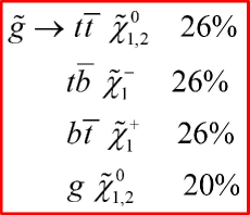
Figure 7: The gluino decay branching fractions for the benchmark point obtained using SDecay.

We have thus re-analyzed the data from CMS, Table 1, for 6 benchmark points with $m_{16}=20$ TeV and different values of the gluino mass.

Analysis	Luminosity	Signal Region	Reference
SS dilepton	10.5	$N_{\mathrm{jet}}\geq 4,\ N_{\mathrm{b-jet}}\geq 2,$	Chatrchyan et al. (2013a)
		$E_{T}^{\mathrm{miss}}>120,\ H_{T}>200$
$\alpha_{T}$ analysis (for Simplified models)	11.7	$N_{\mathrm{jet}}\geq 4,\ N_{\mathrm{b-jet}}=2,\ 775<H_{T}<875$	Chatrchyan et al. (2013b)
(for the benchmark models)		$N_{\mathrm{jet}}\geq 4,\ N_{\mathrm{b-jet}}\geq 2,\ 775<H_{T}<875$
$\Delta\phi$ analysis	19.4	$N_{\mathrm{b-jet}}\geq 3,\ E_{T}^{\mathrm{miss}}>350,\ H_{T}>1000$	Chatrchyan et al. (2013c)

Table 1: The most constraining signal region for each of the analyzes studied in this work. All energies are in units of GeV and luminosity in fb^-1.

We performed a detailed comparison of simplified models, in particular, $BR(\tilde{g}\rightarrow t\ \bar{t}\ \tilde{\chi}^{0}_{1})=$100% and $BR(\tilde{g}\rightarrow b\ \bar{b}\ \tilde{\chi}^{0}_{1})=$100%, vs. the benchmark points from our model Anandakrishnan et al. (2013). We find for the purely hadronic analyzes a 10 - 20% less significant bound, due to the fact there are fewer b-jets as a result of the significant branching fraction, $\tilde{g}\rightarrow g\ \tilde{\chi}^{0}_{1,2}$. The same sign di-lepton bounds are, on the other hand, the most significant. The bottom line is that $m_{\tilde{g}}\geq 1$ TeV.

2.5 Dark Matter

Finally, our LSP is bino-like and thus, using microOmegas, we find it over-closes the universe. One way to solve this problem is to include axions. In this case the bino can decay into an photon and axino. While the dark matter is a linear combination of axinos and axions Baer et al. (2009b).

3 Gauge and Yukawa Unification with Non-Universal Gaugino Masses

This part of the talk is based on the work Anandakrishnan and Raby (2013) and work in progress with Archana Anandakrishnan, B. Charles Bryant and Linda Carpenter. We assume the following GUT scale boundary conditions, namely a universal squark and slepton mass parameter, $m_{16}$, universal cubic scalar parameter, $A_{0}$, “mirage” mediation gaugino masses,

$$M_{i}=\left(1+\frac{g_{G}^{2}b_{i}\alpha}{16\pi^{2}}\log\left(\frac{M_{Pl}}{m_{16}}\right)\right)M_{1/2}$$ (9)

(where $M_{1/2}$ and $\alpha$ are free parameters and $b_{i}=(33/5,1,-3)\;{\rm for}\;i=1,2,3)$. Note, this expression is equivalent to the gaugino masses defined in Choi and Nilles (2007). $\alpha$ in the above expression is related to the $\rho$ in Ref.Lowen and Nilles (2008) as: $\frac{1}{\rho}=\frac{\alpha}{16\pi^{2}}{\rm ln}\frac{M_{PL}}{m_{16}}$. We consider two different cases for non-universal Higgs masses [NUHM] with “just so” Higgs splitting

$$m_{H_{u(d)}}^{2}=m_{10}^{2}-(+)2D$$ (10)

with universal squark and slepton masses, $m_{16}$, or, D-term Higgs splitting, where, in addition, squark and slepton masses are given by

$$m_{a}^{2}=m_{16}^{2}+Q_{a}D,\;\;\{Q_{a}=+1,\{Q,\bar{u},\bar{e}\};-3,\{L,\bar{d}\}\}$$ (11)

with the U(1) D-term, $D$, and SU(5) invariant charges, $Q_{a}$. Note, we take $\mu,\,M_{1/2}<0$. Thus for $\alpha\geq 4$ we have $M_{3}>0,M_{1},M_{2}<0$.

Sector	Third Family Analysis
gauge	$\alpha_{G}$, $M_{G}$, $\epsilon_{3}$
SUSY (GUT scale)	$m_{16}$, $M_{1/2}$, $\alpha$, $A_{0}$, $m_{10}$, $D$
textures	$\lambda$
SUSY (EW scale)	$\tan\beta$, $\mu$
Total #	12

Table 2: The 12 parameters defining the model.

There are 12 parameters and 11 observables, thus we require $\chi^{2}\ll 1$. Nevertheless, since Yukawa unification severely constrains the SUSY breaking sector of the theory we are confident that the SUSY spectrum is robust. Two benchmark points are given in Table 8.

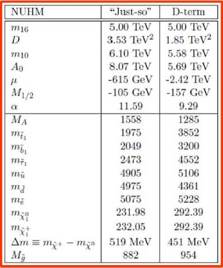
Figure 8: The SUSY spectrum for two benchmark points.

Note, the parameter $\alpha$ which determines the ratio of anomaly mediated and gravity mediated SUSY breaking is large. Thus the spectrum is similar to that of pure anomaly mediation with an almost degenerate neutralino and chargino; both predominantly wino-like. The neutralino and chargino masses in Table 8 are tree level running masses and the factor $\Delta m$ includes the one loop correction to their masses. Note the splitting is of order 500 MeV. As a result the chargino decays predominantly into the neutralino and a single pion. The gluino decay branching fractions for the benchmark point obtained using SDecay is

$$\tilde{g}\rightarrow \{63\%\;\;\tilde{\chi}^{0}\ g,\;{\rm and\ the\ rest\ to}\;\tilde{\chi}^{+}\ b\ \bar{t},\;\tilde{\chi}^{-}\ t\ \bar{b}\} {\rm Just-so\ splitting}$$ (12)

$$\tilde{g}\rightarrow \{56\%\;\;\tilde{\chi}^{+}\ b\ \bar{t},\;\tilde{\chi}^{-}\ t\ \bar{b};\;17\%\;\;\tilde{\chi}^{0}\ t\ \bar{t};\;10\%\;\;\tilde{\chi}^{0}\ b\ \bar{b},\;{\rm and\ the\ rest\ to\ light\ quarks}\} {\rm D-term\ splitting}$$

We are now studying the LHC bounds on the sparticle masses in this model.

3.1 Dark Matter

In this model the dark matter candidate is predominantly wino-like. Therefore, using microOmegas we find, assuming thermal dark matter, that the universe is under-closed. This problem can be avoided if winos are produced non-thermally or with another source of dark matter, such as axions.

4 3 Family Model

The previous results depended solely on SO(10) Yukawa unification for the third family. We now consider a complete three family SO(10) model for fermion masses and mixing, including neutrinos Dermisek and Raby (2005); Dermisek et al. (2006); Albrecht et al. (2007). The model also includes a $D_{3}\times[U(1)\times\mathbb{Z}_{2}\times\mathbb{Z}_{3}]$ family symmetry which is necessary to obtain a predictive theory of fermion masses by reducing the number of arbitrary parameters in the Yukawa matrices. In the rest of this talk we will consider the new results due to the three family analysis. We shall consider the superpotential generating the effective fermion Yukawa couplings. We then perform a global $\chi^{2}$ analysis, including precision electroweak data which now includes both neutral and charged fermion masses and mixing angles.

The superspace potential for the charged fermion sector of this model is given by:

$$W_{ch.fermions}= 16_{3}\ 10\ 16_{3}+16_{a}\ 10\ \chi_{a}$$

$$+\bar{\chi}_{a}\ (M_{\chi}\ \chi_{a}+\ 45\ \frac{\phi_{a}}{\hat{M}}\ 16_{3}\ +\ 45\ \frac{\tilde{\phi}_{a}}{\hat{M}}\ 16_{a}+{\bf A}\ 16_{a})$$

where $45$ is an $SO(10)$ adjoint field which is assumed to obtain a VEV in the B – L direction; and $M$ is a linear combination of an $SO(10)$ singlet and adjoint. Its VEV $M_{0}(1+\alpha X+\beta Y)$ gives mass to Froggatt-Nielsen states. Here $X$ and $Y$ are elements of the Lie algebra of $SO(10)$ with $X$ in the direction of the $U(1)$ which commutes with $SU(5)$ and $Y$ the standard weak hypercharge; and $\alpha$ , $\beta$ are arbitrary constants which are fit to the data.

$$\phi_{a},\quad\tilde{\phi}_{a},\quad A,$$

are $SO(10)$ singlet ’flavon’ fields, and

$$\bar{\chi}_{a},\quad\chi_{a}$$

are a pair of Froggatt-Nielsen states transforming as a $\overline{16}$ and $16$ under $SO(10)$. The ’flavon’ fields are assumed to obtain VEVs of the form

$$\langle\phi_{a}\rangle=\left(\begin{array}[]{c}\phi_{1}\\ \phi_{2}\end{array}\right),\;\;\langle\tilde{\phi}_{a}\rangle=\left(\begin{array}[]{c}0\\ \tilde{\phi}_{2}\end{array}\right).$$ (14)

After integrating out the Froggatt-Nielsen states one obtains the effective fermion mass operators in Fig. 9.

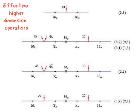
Figure 9: The effective fermion mass operators obtained after integrating out the Froggatt-Nielsen massive states.

We then obtain the Yukawa matrices for up and down quarks, charged leptons and neutrinos given in Fig. 10. These matrices contain 7 real parameters and 4 arbitrary phases.

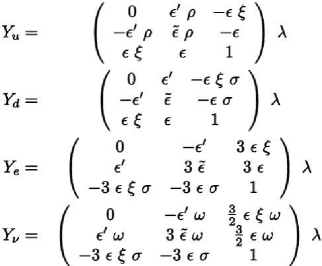
Figure 10: The Yukawa matrices obtained from the effective fermion mass operators after taking into account the flavon VEVs.

Note, the superpotential (Eqn. 4) has many arbitrary parameters. However, at the end of the day the effective Yukawa matrices have many fewer parameters. This is good, because we then obtain a very predictive theory. Also, the quark mass matrices accommodate the Georgi-Jarlskog mechanism, such that $m_{\mu}/m_{e}\approx 9m_{s}/m_{d}$.

We then add 3 real Majorana mass parameters for the neutrino see-saw mechanism. The anti-neutrinos get GUT scale masses by mixing with three $SO(10)$ singlets $\{N_{a},\ a=1,2;\;\;N_{3}\}$ transforming as a $D_{3}$ doublet and singlet respectively. The full superpotential is given by $W=W_{ch.fermions}+W_{neutrino}$ with

$$W_{neutrino}= \overline{16}\left(\lambda_{2}\ N_{a}\ 16_{a}\ +\ \lambda_{3}\ N_{3}\ 16_{3}\right)$$

$$+\;\;\frac{1}{2}\left(S_{a}\ N_{a}\ N_{a}\;\;+\;\;S_{3}\ N_{3}\ N_{3}\right).$$

We assume $\overline{16}$ obtains a VEV, $v_{16}$, in the right-handed neutrino direction, and $\langle S_{a}\rangle=M_{a}$ for $a=1,2$ and $\langle S_{3}\rangle=M_{3}$. The effective neutrino mass terms are given by

$$W=\nu\ m_{\nu}\ \bar{\nu}+\bar{\nu}\ V\ N+\frac{1}{2}\ N\ M_{N}\ N$$ (16)

with

$$V=v_{16}\ \left(\begin{array}[]{ccc}0&\lambda_{2}&0\\ \lambda_{2}&0&0\\ 0&0&\lambda_{3}\end{array}\right),\;M_{N}=diag(M_{1},\ M_{2},\ M_{3})$$ (17)

all assumed to be real. Finally, upon integrating out the heavy Majorana neutrinos we obtain the $3\times 3$ Majorana mass matrix for the light neutrinos in the lepton flavor basis given by

$${\cal M}=U_{e}^{T}\ m_{\nu}\ M_{R}^{-1}\ m_{\nu}^{T}\ U_{e},$$ (18)

where the effective right-handed neutrino Majorana mass matrix is given by:

$$M_{R}=V\ M_{N}^{-1}\ V^{T}\ \equiv\ {\rm diag}(M_{R_{1}},M_{R_{2}},M_{R_{3}}),$$ (19)

with

$$M_{R_{1}}=(\lambda_{2}\ v_{16})^{2}/M_{2},\quad M_{R_{2}}=(\lambda_{2}\ v_{16})^{2}/M_{1},\quad M_{R_{3}}=(\lambda_{3}\ v_{16})^{2}/M_{3}.$$ (20)

5 Global $\chi^{2}$ analysis

Just in the fermion mass sector we can see that the theory is very predictive. We have 15 charged fermion and 5 neutrino low energy observables given in terms of 11 arbitrary Yukawa parameters and 3 Majorana mass parameters. Hence there are 6 degrees of freedom in this sector of the theory. However in order to include the complete MSSM sector we perform the global $\chi^{2}$ analysis with 24 arbitrary parameters at the GUT scale given in Table 3. Note, this is to be compared to the 27 arbitrary parameters in the Standard Model or the 32 parameters in the CMSSM.

Table 3: Parameters entering the global $\chi^{2}$ analysis.

$Sector$	#	$Parameters$
$gauge$	$3$	$\alpha_{G},\ M_{G},\ \epsilon_{3}$
$SUSY\ (GUTscale)$	$5$	$m_{16},\ M_{1/2},\ A_{0},\ m_{H_{u}},\ m_{H_{d}}$
$textures$	$11$	$\lambda,\ \epsilon,\ \epsilon^{\prime},\ \rho,\ \sigma,\ \tilde{\epsilon},\ \xi$
$neutrino$	$3$	$M_{R_{1}},\ M_{R_{2}},\ M_{R_{3}}$
$SUSY\ (EWscale)$	$2$	$\mu,\ \tan\beta$

In this work we have decided to extend the analysis of Albrecht et al. to values of $m_{16}\geq 10$ TeV, including more low energy observables such as the light Higgs mass, the neutrino mixing angle $\theta_{13}$ and lower bounds on the gluino and squark masses coming from recent data. We perform a three family global $\chi^{2}$ analysis. We are using the code, maton, developed by Radovan Dermisek to renormalize the parameters in the theory from the GUT scale to the weak scale, perform electroweak symmetry breaking and calculate squark, slepton, gaugino masses, as well as quark and lepton masses and mixing angles. We also use the Higgs code of Pietro Slavich (suitably revised for our particular scalar spectrum) to calculate the light Higgs mass and SUSY_Flavor_v2.0 Crivellin et al. (2012) to evaluate flavor violating B decays.

There are 24 arbitrary parameters defined mostly at the GUT scale and run down to the weak scale where the $\chi^{2}$ function is evaluated. However the value of $m_{16}$ has been kept fixed in our analysis, so that we can see the dependence of $\chi^{2}$ on this input parameter. Thus with 23 arbitrary parameters we fit 36 observables, giving 13 degrees of freedom. The $\chi^{2}$ function has been minimized using the CERN package, MINUIT.

Initial parameters for benchmark point with $m_{16}=20$ TeV (see Table 4).
(1/$\alpha_{G},\,M_{G},\,\epsilon_{3}$) = ($25.90,\,3.13\times 10^{16}$ GeV, $\,-1.45$ %),
($\lambda,\,\lambda\epsilon,\,\sigma,\,\lambda\tilde{\epsilon},\,\rho,\,\lambda\epsilon^{\prime},\,\lambda\epsilon\xi$) = ($0.60,\,0.031,\,1.14,\,0.0049,\,0.070,\,-0.0019,\,0.0038$),
($\Phi_{\sigma},\,\Phi_{\tilde{\epsilon}},\,\Phi_{\rho},\,\Phi_{\xi}$) = ($0.533,\,0.548,\,3.936,\,3.508$) rad,
($m_{16},\,M_{1/2},\,A_{0},\,\mu(M_{Z})$) = ($20000,\,168,\,-41087,\,1163.25$) GeV,
($(m_{H_{d}}/m_{16})^{2},\,(m_{H_{u}}/m_{16})^{2},\,\tan\beta$) = ($1.85,\,1.61,\,49.82$)
($M_{R_{3}},\,M_{R_{2}},\,M_{R_{1}}$) = ($3.2\times 10^{13}$ GeV, $\,6.1\times 10^{11}$ GeV, $\,0.9\times 10^{10}$ GeV)

The fit is quite good with $\chi^{2}/d.o.f.=2$. However, note that we have not taken into account correlations in the data, so we will just use $\chi^{2}$ as a indicator of the rough goodness of the fit.

Table 4: Benchmark point with ${\boldsymbol{m_{16}=20\;{\rm TeV}}}$.

Observable	Fit value	Exp value	Pull	Sigma
$M_{Z}$	91.1876	91.1876	0.0000	0.4559
$M_{W}$	80.5452	80.3850	0.3982	0.4022
$1/\alpha_{em}$	137.0725	137.0360	0.0533	0.6852
$G_{\mu}\times 10^{5}$	1.1713	1.1664	0.4250	0.0117
$\alpha_{3}$	0.1184	0.1184	0.0467	0.0009
$M_{t}$	174.0184	173.5000	0.3916	1.3238
$m_{b}(m_{b})$	4.1849	4.1800	0.1334	0.0366
$M_{\tau}$	1.7755	1.7768	0.1462	0.0089
$m_{c}(m_{c})$	1.2547	1.2750	0.7876	0.0258
$m_{s}$	0.0964	0.0950	0.2807	0.0050
$m_{d}/m_{s}$	0.0692	0.0526	2.9891	0.0055
$1/Q^{2}$	0.0018	0.0019	0.4749	0.0001
$M_{\mu}$	0.1056	0.1057	0.1049	0.0005
$M_{e}\times 10^{4}$	5.1122	5.1100	0.0862	0.0255
$|V_{us}|$	0.2243	0.2252	0.5964	0.0014
$|V_{cb}|$	0.0415	0.0406	0.4511	0.0020
$|V_{ub}|\times 10^{3}$	3.2023	3.7700	0.6678	0.8502
$|V_{td}|\times 10^{3}$	8.9819	8.4000	0.9675	0.6015
$|V_{ts}|$	0.0407	0.0429	0.8518	0.0026
$\text{sin}2\beta$	0.6304	0.6790	2.3959	0.0203
$\epsilon_{K}$	0.0023	0.0022	0.3823	0.0002
$\Delta M_{Bs}/\Delta M_{Bd}$	39.4933	35.0600	0.6311	7.0246
$\Delta M_{Bd}\times 10^{13}$	3.9432	3.3370	0.9072	0.6682
$m^{2}_{21}\times 10^{5}$	7.5126	7.5450	0.0593	0.5463
$m^{2}_{31}\times 10^{3}$	2.4828	2.4800	0.0135	0.2104
$\text{sin}^{2}\theta_{12}$	0.2949	0.3050	0.2880	0.0350
$\text{sin}^{2}\theta_{23}$	0.5156	0.5050	0.0640	0.1650
$\text{sin}^{2}\theta_{13}$	0.0131	0.0230	1.4134	0.0070
$M_{h}$	124.07	125.30	0.4010	3.0676
$BR(B\rightarrow X_{s}\gamma)\times 10^{4}$	3.4444	3.4300	0.0088	1.6374
$BR(B_{s}\rightarrow\mu^{+}\mu^{-})\times 10^{9}$	1.6210	3.2000	0.9682	1.6308
$BR(B_{d}\rightarrow\mu^{+}\mu^{-})\times 10^{10}$	1.0231	8.1000	0.0000	5.2559
$BR(B\rightarrow\tau\nu)\times 10^{5}$	6.3855	16.6000	1.1436	8.9320
$BR(B\rightarrow K^{*}\mu^{+}\mu^{-})$(low) $\times 10^{8}$	5.1468	19.7000	1.2123	12.0051
$BR(B\rightarrow K^{*}\mu^{+}\mu^{-})$(high) $\times 10^{8}$	7.7469	12.0000	0.5839	7.2835
$q_{0}^{2}(B\rightarrow K^{*}\mu^{+}\mu^{-})$	4.5168	4.9000	0.2945	1.3009
Total $\chi^{2}$			26.5812

In Table 5 we see that the value of $\chi^{2}$ decreases as $m_{16}$ increases, but our analysis shows that the $m_{16}\sim 20$ TeV minimizes $\chi^{2}$, i.e. we have found that $\chi^{2}$ slowly increases for $m_{16}>20$ TeV. Note, we are able to fit the neutrino masses and mixing angles quite well. The two large mixing angles are due to the hierarchy of right-handed neutrino masses. The biggest discrepancy is for the angle $\theta_{13}$. We obtain a value which is closer to 6^∘, rather than the observed value of order 9^∘. In Table 6 we present results for lepton flavor and CP violation.

$m_{16}$	20 TeV	30 TeV
$\chi^{2}$	26.58	29.48
$M_{A}$	1651	2036
$m_{\tilde{t}_{1}}$	3975	5914
$m_{\tilde{b}_{1}}$	5194	7660
$m_{\tilde{\tau}_{1}}$	7994	11620
$m_{\tilde{\chi}^{0}_{1}}$	137	167
$m_{\tilde{\chi}^{+}_{1}}$	279	351
$M_{\tilde{g}}$	851	1004
$\chi^{2}/{\rm dof}$	2	2.2

Table 5: SUSY Spectrum corresponding to two benchmark points. The first two generation scalars have mass of the order of $m_{16}$.

	Current Limit	10 TeV	15 Te V	20 TeV	25 TeV	30 TeV
e EDM $\times 10^{28}$	$<10.5\ e\ cm$	$-0.224$	$-0.0408$	$-0.0173$	$-0.0113$	$-0.0084$
$\mu$ EDM $\times 10^{28}$	$(-0.1\pm 0.9)\times 10^{9}\ e\ cm$	$34.6$	$6.23$	$3.04$	$1.77$	$1.20$
$\tau$ EDM $\times 10^{28}$	$-0.220-0.45\times 10^{12}\ e\ cm$	$-2.09$	$-0.394$	$-0.185$	$-0.109$	$-0.0732$
BR$(\mu\rightarrow e\gamma)\times 10^{12}$	$<2.4$	$5.09$	$1.23$	$0.211$	$0.0937$	$0.0447$
BR$(\tau\rightarrow e\gamma)\times 10^{12}$	$<3.3\times 10^{4}$	$58.8$	$13.9$	$2.40$	$1.04$	$0.502$
BR$(\tau\rightarrow\mu\gamma)\times 10^{8}$	$<4.4$	$1.75$	$0.498$	$0.0837$	$0.0385$	$0.0182$
sin $\delta$		-0.60	-0.87	-0.27	-0.42	-0.53

Table 6: Predictions from the full three family analysis. The dipole moments and branching ratios were calculated using susy_flavor.

6 Conclusion and plans for the future

We have presented an analysis of a theory satisfying Yukawa unification and large $\tan\beta$. The results are encouraging. We find SO(10) Yukawa unification is still alive after LHC 7, 8! Some of the good features are -

• gauge coupling unification is satisfied

• the Higgs mass is of order 125 GeV and Standard Model-like

• there is an inverted scalar mass hierarchy

• for universal gaugino masses we find $m_{\tilde{g}}\geq 1$ TeV and $m_{\tilde{g}}\leq 3$ TeV for $m_{16}\leq 30$ TeV

• for non-universal gaugino masses, the lightest chargino and neutralino are almost degenerate.

Finally, in collaboration with Anandakrishnan, Bryant and Carpenter, we are continuing to analyze the LHC phenomenology of models with effective “mirage” mediation.

References

- Hall et al. (1994) L. J. Hall, R. Rattazzi, and U. Sarid, Phys.Rev. D50, 7048–7065 (1994), hep-ph/9306309.
- Carena et al. (1994) M. S. Carena, M. Olechowski, S. Pokorski, and C. Wagner, Nucl.Phys. B426, 269–300 (1994), hep-ph/9402253.
- Blazek et al. (1995) T. Blazek, S. Raby, and S. Pokorski, Phys.Rev. D52, 4151–4158 (1995), hep-ph/9504364.
- Blazek et al. (2002a) T. Blazek, R. Dermisek, and S. Raby, Phys.Rev.Lett. 88, 111804 (2002a), hep-ph/0107097.
- Blazek et al. (2002b) T. Blazek, R. Dermisek, and S. Raby, Phys.Rev. D65, 115004 (2002b), hep-ph/0201081.
- Baer and Ferrandis (2001) H. Baer, and J. Ferrandis, Phys.Rev.Lett. 87, 211803 (2001), hep-ph/0106352.
- Auto et al. (2003) D. Auto, H. Baer, C. Balazs, A. Belyaev, J. Ferrandis, et al., JHEP 0306, 023 (2003), hep-ph/0302155.
- Tobe and Wells (2003) K. Tobe, and J. D. Wells, Nucl.Phys. B663, 123–140 (2003), hep-ph/0301015.
- Dermisek et al. (2003) R. Dermisek, S. Raby, L. Roszkowski, and R. Ruiz De Austri, JHEP 0304, 037 (2003), hep-ph/0304101.
- Dermisek et al. (2005) R. Dermisek, S. Raby, L. Roszkowski, and R. Ruiz de Austri, JHEP 0509, 029 (2005), hep-ph/0507233.
- Baer et al. (2008a) H. Baer, S. Kraml, S. Sekmen, and H. Summy, JHEP 0803, 056 (2008a), 0801.1831.
- Baer et al. (2008b) H. Baer, S. Kraml, S. Sekmen, and H. Summy, JHEP 0810, 079 (2008b), 0809.0710.
- Baer et al. (2009a) H. Baer, S. Kraml, and S. Sekmen, JHEP 0909, 005 (2009a), 0908.0134.
- Badziak et al. (2011) M. Badziak, M. Olechowski, and S. Pokorski, JHEP 1108, 147 (2011), 1107.2764.
- Gogoladze et al. (2012) I. Gogoladze, Q. Shafi, and C. S. Un, JHEP 1208, 028 (2012), 1112.2206.
- Anandakrishnan et al. (2012) A. Anandakrishnan, S. Raby, and A. Wingerter (2012), 1212.0542.
- Anandakrishnan and Raby (2013) A. Anandakrishnan, and S. Raby (2013), 1303.5125.
- Anandakrishnan et al. (2013) A. Anandakrishnan, B. C. Bryant, S. Raby, and A. Wingerter (2013), 1307.7723.
- Bagger et al. (2000) J. A. Bagger, J. L. Feng, N. Polonsky, and R.-J. Zhang, Phys.Lett. B473, 264–271 (2000), hep-ph/9911255.
- Aaij et al. (2013) R. Aaij, et al., Eur.Phys.J. C73, 2373 (2013), 1208.3355.
- Albrecht et al. (2007) M. Albrecht, W. Altmannshofer, A. J. Buras, D. Guadagnoli, and D. M. Straub, JHEP 0710, 055 (2007), 0707.3954.
- Carena et al. (1996) M. S. Carena, M. Quiros, and C. Wagner, Nucl.Phys. B461, 407–436 (1996), hep-ph/9508343.
- Aaij et al. (2012) R. Aaij, et al. (2012), 1211.2674.
- 1244669 (2013) 1244669 (2013), 1307.7135.
- Chatrchyan et al. (2013a) S. Chatrchyan, et al., JHEP 1303, 037 (2013a), 1212.6194.
- Chatrchyan et al. (2013b) S. Chatrchyan, et al. (2013b), 1303.2985.
- Chatrchyan et al. (2013c) S. Chatrchyan, et al. (2013c), 1305.2390.
- Baer et al. (2009b) H. Baer, M. Haider, S. Kraml, S. Sekmen, and H. Summy, JCAP 0902, 002 (2009b), 0812.2693.
- Choi and Nilles (2007) K. Choi, and H. P. Nilles, JHEP 0704, 006 (2007), hep-ph/0702146.
- Lowen and Nilles (2008) V. Lowen, and H. P. Nilles, Phys.Rev. D77, 106007 (2008), 0802.1137.
- Dermisek and Raby (2005) R. Dermisek, and S. Raby, Phys.Lett. B622, 327–338 (2005), %****␣raby.SO_10_.CETUP.bbl␣Line␣125␣****hep-ph/0507045.
- Dermisek et al. (2006) R. Dermisek, M. Harada, and S. Raby, Phys.Rev. D74, 035011 (2006), hep-ph/0606055.
- Crivellin et al. (2012) A. Crivellin, J. Rosiek, P. Chankowski, A. Dedes, S. Jaeger, et al. (2012), 1203.5023.