A UV complete model for radiative seesaw and electroweak baryogenesis based on the SUSY gauge theory

Abstract

In a class of supersymmetric gauge theories with asymptotic freedom, the low energy effective theory below the confinement scale is described by the composite superfields of the fundamental representation fields. Based on the supersymmetric gauge theory with $N_{c}=2$ and $N_{f}=3$ with an additional unbroken $Z_{2}$ symmetry, we propose a new model where neutrino masses, dark matter, and baryon asymmetry of the Universe can be simultaneously explained by physics below the confinement scale. This is an example for the ultraviolet complete supersymmetric extension of so-called radiative seesaw scenarios with first-order phase transition required for successful electroweak baryogenesis. We show that there are benchmark points where all the neutrino data, the lepton flavor violation data, and the LHC data are satisfied. We also briefly discuss Higgs phenomenology in this model.

I Introduction

The discovery of the Higgs bosonHiggsLHC and measurements of its propertiesHiggsPropLHC at the LHC provide us a clue to explore the essence of electroweak symmetry breaking, which is possibly described by new physics beyond the Standard Model (SM) at the TeV scale. On the other hand, new physics is required to explain phenomena such as neutrino oscillation, existence of dark matter (DM) and baryon asymmetry of the Universe (BAU). If the origins of these phenomena are related to the essence of the Higgs sector, they should also arise from new physics at the TeV scale. In such cases, their origins can be found at current and future collider experiments.

For example, let us consider the scenario of generating neutrino masses by the quantum effectzee ; zeebabu ; ma ; knt ; aks ; aks2 , in which tiny neutrino masses are explained by perturbation of the dynamics at the TeV scale. There is a class of models with right-handed (RH) neutrinos which are assigned the odd-parity under an additional $Z_{2}$ symmetryma ; knt ; aks ; aks2 . The $Z_{2}$ symmetry forces the neutrino masses to be generated only at the quantum level, giving loop suppression to the neutrino masses. Also, the lightest $Z_{2}$-odd particle can be a DM candidate if the $Z_{2}$ symmetry is unbroken. We call such scenarios as radiative seesaw scenarios. The Ma model is the simplest one in such a scenario, in which neutrino masses are generated at the one-loop level by the contribution of an extra $Z_{2}$-odd $\text{SU(2)}_{L}$ scalar doublet (inert doublet) and $Z_{2}$-odd RH neutrinosma . A neutral component of the inert doublet field or the lightest RH neutrino can be the DM. On the other hand, in the Aoki-Kanemura-Seto model (the AKS model)aks ; aks2 , where $Z_{2}$-odd charged and neutral singlet scalars as well as $Z_{2}$-odd RH neutrinos are added to a two Higgs doublet model, neutrino masses are induced at the three-loop level and at the same time the lightest $Z_{2}$-odd particle (the $Z_{2}$-odd neutral singlet or the RH neutrino) can be the DM. In addition, in this model, electroweak baryogenesis can be simultaneously realized due to strong first-order electroweak phase transition(1stOPT) and the CP violating phases in the Higgs sectorEWBG .

These models of radiative seesaw scenarios have been introduced as purely phenomenological models. For example, in the AKS model, some of the coupling constants in the Higgs sector and the new Yukawa coupling constants for the RH neutrinos are of order one in order to satisfy the condition of strong 1stOPT and also to reproduce the neutrino data. Consequently, these coupling constants blow up as the energy scale increases and the Landau pole appears at the point much below the Planck scale or the GUT scale, and the model is well-defined only below the Landau poleaky . This suggests that the model is a low energy effective description of a more fundamental theory above the cutoff scale which corresponds to the Landau pole. It is then a very interesting question what kind of a fundamental theory can lead to such a low energy effective theory.

In this paper, we propose a concrete model of the fundamental theory whose low-energy description gives a phenomenological modelaks of radiative seesaw scenarios with electroweak baryogenesis. In this model, the origin of the Higgs force above the cutoff scale of the low energy theory is a new gauge interaction with asymptotic freedom. In order to describe this picture, we consider the supersymmetric (SUSY) SU($N_{c}$) theory with $N_{f}$ flavorsfatHiggs ; fatbutlight . For $N_{f}=N_{c}+1$, confinement occurs at an infrared (IR) scale $\Lambda_{H}$IntrSei . We here consider the simplest case with $N_{c}=2$ and $N_{f}=3$. In the low-energy effective theory below the confinement scale $\Lambda_{H}$, Higgs superfields $H_{ij}(\sim T_{i}T_{j})$ appear as the composite states of the fundamental superfields $T_{i}\;(i=1,\cdots,6)$ which are doublets of the $\text{SU}(2)_{H}$ gauge symmetrycomposite . In order to realize radiative seesaw scenarios in the low-energy effective theory, we add elementary RH neutrino superfields $N_{i}^{c}\;(i=1,\cdots 3$) to the model. We further impose a $Z_{2}$ symmetry to the model assuming that $N_{i}^{c}$ and some of $T_{i}$’s are $Z_{2}$-odd. Below the confinement scale, the symmetries of the model are $\text{SU}(3)_{C}\times\text{SU}(2)_{L}\times\text{U}(1)_{Y}\times Z_{2}$, under which fifteen Higgs superfields appearKSYam . All the scalar particles required in the AKS model are included in these fifteen Higgs superfields. It is quite interesting that the complicated particle content of the AKS model is predicted by this $\text{SU}(2)_{H}\times Z_{2}$ theory above the cutoff scale without any artificial assumption.

The condition of strongly 1stOPT, $\varphi_{c}/T_{c}\gtrsim 1$, which is required for successful electroweak baryogenesis determines the size of the coupling constants of the Higgs potential at the electroweak scale. This property commonly results in the enhanced triple Higgs boson constant KOS ; GroSer . The electroweak baryogenesis scenario can partially be tested by measuring the triple Higgs boson coupling at future collider experiments. By the renormalization group equation (RGE) analysis of the coupling constant, the scale of the Landau pole is evaluated as $\mathcal{O}(10)\text{TeV}$KSS ; KSSY , which is identical to the confinement scale $\Lambda_{H}$ under the Na$\ddot{\i}$ve Dimensional Analysis (NDA)nda .

In our model, the lightest $Z_{2}$-odd particle in the effective theory can be a DM candidate as in usual radiative seesaw scenarios. If the $R$-parity is also imposed, there are two discrete symmetries, and a rich possibility for the multi-component DM scenario occursmultiDM . In this paper, however, we do not specify the scenario of DM. Detailed analysis for the multi-component DM scenario will be performed in our model elsewherefuture .

We show that the neutrino masses are generated at the loop level in the low-energy effective theory of our model. It contains diagrams of both the Ma model and the AKS model. We find benchmark points in the parameter space where all the current experimental data for Higgs bosons, neutrino data, constraints of lepton flavor violation processes and the condition of strongly 1stOPT are satisfied. We also discuss the possibility of testing this model at current and future collider experiments.

II Model based on SUSY strong dynamics

In this section, we will briefly review a SUSY model with $\text{SU(2)}_{H}\times Z_{2}$ symmetry and six chiral superfields, denoted by $T_{i}\ (i=1,\cdots,6)$, which are doublets of the $\text{SU}(2)_{H}$ gauge symmetry. The superfields $T_{i}$’s are also charged under the SM gauge groups $\text{SU}(2)_{L}\times U(1)_{Y}$. The SM charges and $Z_{2}$ parity assignments on $T_{i}$’s are given in Table 1.

Table 1: The SM charges and $Z_{2}$ parity assignments on the $\text{SU}(2)_{H}$ doublets $T_{i}$.

Superfield	$\text{SU}(3)_{C}$	$\text{SU}(2)_{L}$	$\text{U}(1)_{Y}$	$Z_{2}$
$\left(\begin{array}[]{c}T_{1}\\ T_{2}\end{array}\right)$	1	2	0	$+1$
$T_{3}$	1	1	+1/2	$+1$
$T_{4}$	1	1	$-$1/2	$+1$
$T_{5}$	1	1	+1/2	$-1$
$T_{6}$	1	1	$-$1/2	$-1$

The tree-level superpotential respecting all the gauge symmetries and the $Z_{2}$ parity is written as

$$W_{\text{tree}} =m_{1}T_{1}T_{2}+m_{3}T_{3}T_{4}+m_{5}T_{5}T_{6}\;.$$ (1)

The SU(2)_H gauge coupling becomes non-perturbative at an IR scale, denoted by $\Lambda_{H}$. Below the scale $\Lambda_{H}$, the theory is described in terms of composite chiral superfields, $H_{ij}^{\prime}=T_{i}T_{j}\ (i\neq j)$, which are singlets of SU(2)_H. We have the following dynamically generated superpotential below $\Lambda_{H}$:

$$W_{\text{dyn}} =-\frac{1}{\Lambda^{3}}\epsilon^{ijklmn}H_{ij}^{\prime}H_{kl}^{\prime}H_{mn}^{\prime}\;,$$ (2)

where $\Lambda$ is a dynamically generated scaleIntrSei . The total effective superpotential is simply the sum of $W_{\text{dyn}}$ and $W_{\text{tree}}$:

$$W_{\text{eff}} =W_{\text{dyn}}+W_{\text{tree}}=W_{\text{dyn}}+m_{1}H_{12}^{\prime}+m_{3}H_{34}^{\prime}+m_{5}H_{56}^{\prime}\;.$$ (3)

We cannot determine the normalization for the dynamically generated superpotential. The effective Kähler potential below the scale $\Lambda_{H}$ is also undetermined, and so is the canonical normalization for the mesonic superfields. However,the NDA suggests the following form of the effective Kähler potential and normalization for the effective superpotential at the scale $\Lambda_{H}$nda :

$$K_{\text{eff}}[\Lambda_{H}] \simeq\frac{1}{16\pi^{2}\Lambda_{H}^{2}}H_{ij}^{\prime\dagger}H_{ij}^{\prime}\;,$$ (4)

$$W_{\text{eff}}[\Lambda_{H}] \simeq-\frac{1}{16\pi^{2}\Lambda_{H}^{3}}\epsilon^{ijklmn}H_{ij}^{\prime}H_{kl}^{\prime}H_{mn}^{\prime}+m_{1}H_{12}^{\prime}+m_{3}H_{34}^{\prime}+m_{5}H_{56}^{\prime}\;.$$ (5)

The canonically normalized mesonic superfields $H_{ij}$ at the scale $\Lambda_{H}$ are then given by

$$H_{ij} \simeq\frac{1}{4\pi\Lambda_{H}}H_{ij}^{\prime}\;,$$ (6)

and the superpotential at the scale $\Lambda_{H}$ is rewritten as

$$W_{\text{eff}}[\Lambda_{H}]\simeq 4\pi\epsilon^{ijklmn}H_{ij}H_{kl}H_{mn}+4\pi\Lambda_{H}m_{1}H_{12}+4\pi\Lambda_{H}m_{3}H_{34}+4\pi\Lambda_{H}m_{5}H_{56}\;.$$ (7)

The basic setup explained above is the same as the one in the minimal SUSY fat Higgs modelfatHiggs . In general, fifteen mesonic superfields $H_{ij}$ appear in the low-energy effective theory of the fundamental $\text{SU}(2)_{H}$ gauge theory with 3 flavors. In the minimal SUSY fat Higgs model, the superfields in the low-energy effective theory are made to be identical to those in the nMSSMnMSSM by introducing several $\text{SU}(2)_{H}$ singlet superfields which give masses as large as $\Lambda_{H}$ to ten of the fifteen mesonic superfields. On the other hand, in our model, we do not introduce such additional singlets and thus all the fifteen mesonic chiral superfields remain in the effective theory below $\Lambda_{H}$.

We identify the fifteen mesonic chiral superfields, $H_{ij}$, with the MSSM Higgs doublets, $H_{u},\ H_{d}$, and the exotic chiral superfields in an extended Higgs sector, as

$$H_{u} \equiv\left(\begin{array}[]{c}H_{13}\\ H_{23}\end{array}\right)\;,\quad H_{d}\equiv\left(\begin{array}[]{c}H_{14}\\ H_{24}\end{array}\right)\;,\quad\Phi_{u}\equiv\left(\begin{array}[]{c}H_{15}\\ H_{25}\end{array}\right)\;,\quad\Phi_{d}\equiv\left(\begin{array}[]{c}H_{16}\\ H_{26}\end{array}\right)\;,\quad$$ (16)

$$N \equiv H_{56}\;,\quad N_{\Phi}\equiv H_{34}\;,\quad N_{\Omega}\equiv H_{12}\;,\quad$$

$$\Omega^{+} \equiv H_{35}\;,\quad\Omega^{-}\equiv H_{46}\;,\quad\zeta\equiv H_{36}\;,\quad\eta\equiv H_{45}\;.\quad$$ (17)

The SM charge and $Z_{2}$ parity of these Higgs superfields are summarized in Table 2.

Table 2: The field contents of the Higgs sector below $\Lambda_{H}$.

Field	$\text{SU}(3)_{C}$	$\text{SU}(2)_{L}$	$\text{U}(1)_{Y}$	$Z_{2}$
$H_{u}$	1	2	+1/2	$+1$
$H_{d}$	1	2	$-$1/2	$+1$
$\Phi_{u}$	1	2	+1/2	$-1$
$\Phi_{d}$	1	2	$-$1/2	$-1$
$\Omega^{+}$	1	1	+1	$-1$
$\Omega^{-}$	1	1	$-$1	$-1$
$N$, $N_{\Phi}$, $N_{\Omega}$	1	1	0	$+1$
$\zeta$, $\eta$	1	1	0	$-1$

With these fields, the superpotential in Eq. (7) is rewritten as

$$W_{\text{eff}} =\hat{\lambda}\left\{N(H_{u}H_{d}+v_{0}^{2})+N_{\Phi}(\Phi_{u}\Phi_{d}+v_{\Phi}^{2})+N_{\Omega}(\Omega^{+}\Omega^{-}+v_{\Omega}^{2})\right.$$

$$-\left.NN_{\Phi}N_{\Omega}-N_{\Omega}\zeta\eta+\zeta H_{d}\Phi_{u}+\eta H_{u}\Phi_{d}-\Omega^{+}H_{d}\Phi_{d}-\Omega^{-}H_{u}\Phi_{u}\right\}\;.$$ (18)

After the $Z_{2}$-even neutral fields $N$, $N_{\Phi}$, and $N_{\Omega}$ get vacuum expectation values (vev’s), the relevant terms of the effective superpotential are given byKSYam ; KSSY

$$W_{\text{eff}}= -\mu H_{u}H_{d}-\mu_{\Phi}\Phi_{u}\Phi_{d}-\mu_{\Omega}(\Omega^{+}\Omega^{-}-\zeta\eta)$$

$$+\hat{\lambda}\left\{H_{d}\Phi_{u}\zeta+H_{u}\Phi_{d}\eta-H_{u}\Phi_{u}\Omega^{-}-H_{d}\Phi_{d}\Omega^{+}\right\}\;.$$ (19)

The relevant soft SUSY breaking terms are given by

$${\cal L}_{H} =-m_{H_{u}}^{2}H_{u}^{\dagger}H_{u}-m_{H_{d}}^{2}H_{d}^{\dagger}H_{d}-m_{\Phi_{u}}^{2}\Phi_{u}^{\dagger}\Phi_{u}-m_{\Phi_{d}}^{2}\Phi_{d}^{\dagger}\Phi_{d}$$

$$-m_{\Omega^{+}}^{2}\Omega^{+\,\dagger}\Omega^{+}-m_{\Omega^{-}}^{2}\Omega^{-\,\dagger}\Omega^{-}-m_{\zeta}^{2}\zeta^{\dagger}\zeta-m_{\eta}^{2}\eta^{\dagger}\eta$$

$$-\left\{B\mu H_{u}H_{d}+B_{\Phi}\mu_{\Phi}\Phi_{u}\Phi_{d}+B_{\Omega}\mu_{\Omega}(\Omega^{+}\Omega^{-}+\zeta\eta)+\text{h.c.}\right\}$$

$$-\left\{A_{\zeta}H_{d}\Phi_{u}\zeta+A_{\eta}H_{u}\Phi_{d}\eta+A_{\Omega^{-}}H_{u}\Phi_{u}\Omega^{-}+A_{\Omega^{+}}H_{d}\Phi_{d}\Omega^{+}+\text{h.c.}\right\}$$

$$-\left\{m_{\zeta\eta}^{2}\eta^{\dagger}\zeta+\frac{B_{\zeta}^{2}}{2}\zeta^{2}+\frac{B_{\eta}^{2}}{2}\eta^{2}+\text{h.c.}\right\}\;.$$ (20)

The coupling constant $\hat{\lambda}$ and the cutoff scale $\Lambda_{H}$ are related through the NDA. Under the assumption of the NDA, the coupling constant $\hat{\lambda}$ becomes non-perturbative at $\Lambda_{H}$ as $\hat{\lambda}\simeq 4\pi$. The value of $\hat{\lambda}$ at the cutoff scale $\Lambda_{H}$ is connected to those at low energy scales by RGE. Therefore, the cutoff scale $\Lambda_{H}$ can be predicted from the value of the coupling constant $\hat{\lambda}$ at the electroweak scale, $\hat{\lambda}(\mu_{\text{EW}})$. In this paper, we constrain the range of $\Lambda_{H}$ by requiring that the coupling constant $\hat{\lambda}(\mu_{\text{EW}})$ satisfies the condition of strongly 1stOPT, $\varphi_{c}/T_{c}\gtrsim 1$, which is one of the conditions for successful electroweak baryogenesisEWBG . In general, non-decoupling quantum effects of additional scalar fields make the order of electroweak phase transition strong. In Refs. KSS ; KSSY , some of the extra scalar fields such as $\Phi_{u}$, $\Phi_{d}$, $\Omega^{+}$, $\Omega^{-}$ $\zeta$, and $\eta$ significantly contribute to make the order of electroweak phase transition stronger, when the coupling $\hat{\lambda}$ satisfies $\hat{\lambda}(\mu_{\text{EW}})\gtrsim 1.6$ at the electroweak scale. Correspondingly, the Landau pole appears at the scale around ten TeV.

III Loop induced neutrino masses

We will show that radiative seesaw scenariosaks ; ma are realized in the low energy effective theory of the $\text{SU}(2)_{H}\times Z_{2}$ model by adding $Z_{2}$-odd RH neutrino superfields $N^{c}_{i}$. The superpotential relevant to the neutrino sector is given by

$$W_{N}= y_{N}^{ij}N^{c}_{i}L_{j}\Phi_{u}+h_{N}^{ij}N^{c}_{i}E^{c}_{j}\Omega^{-}+\frac{M_{i}}{2}N^{c}_{i}N^{c}_{i}\;,$$ (21)

where $E^{c}_{i}$ and $L_{i}$ are the RH charged lepton chiral superfields and the lepton doublet chiral superfield, respectively, and the basis of the lepton fields are taken such that both the mass matrix for the $N^{c}_{i}$ and the charged lepton Yukawa matrix are real and diagonal. Notice that the $Z_{2}$ parity prohibits the neutrino Yukawa interactions as $N^{c}_{i}L_{j}H_{u}$ which give neutrino masses at the tree level, so that the type I seesaw mechanism does not work.

In our model, the neutrino masses are radiatively generated by (I) one-loop diagrams and (II) three-loop diagrams. The one-loop diagrams correspond to the coupling constants $y_{N}^{ij}$, and the three-loop diagrams correspond to the coupling constants $h_{N}^{ij}$.

III.1 One-loop contributions

The one-loop diagrams which contribute to the neutrino mass matrix are shown in Fig. 1. These diagrams correspond to the SUSY extension of the Ma modelma . Such mass terms as $\eta^{2}$ or $\zeta^{2}$ cannot be written in the superpotential of our model due to the SUSY dynamics at $\Lambda_{H}$, so that the loop diagrams with RH sneutrinos and $Z_{2}$-odd fermions do not contribute. The contributions to the mass matrix are calculated as

$$m_{ij}^{(\text{I})}=\frac{(y_{N})^{ki}(y_{N})^{kj}}{(4\pi)^{2}}\left\{(O_{0})^{1\alpha}(O_{0})^{1\alpha}M_{k}-(O_{0})^{5\alpha}(O_{0})^{5\alpha}M_{k}\right\}\bar{B}_{0}(m_{\Phi_{\alpha}}^{2},M_{k}^{2})\;,$$ (22)

where the loop function $\bar{B}_{0}$ is given as

$$\bar{B}_{0}(m_{1}^{2},m_{2}^{2})=-\frac{m_{1}^{2}\ln m_{1}^{2}-m_{2}^{2}\ln m_{2}^{2}}{m_{1}^{2}-m_{2}^{2}}\;,$$ (23)

and the matrix $O_{0}$ is the mixing matrix for the $Z_{2}$-odd neutral scalars (see Appendix A).

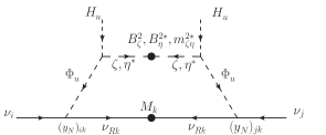
Figure 1: A one-loop diagram which contributes to the neutrino mass matrix.

III.2 Three-loop contributions

The three-loop diagrams which contribute to the neutrino mass matrix are shown in Fig. 2. The contributions are calculated as

$$m_{ij}^{\text{(II)}}= \frac{\hat{\lambda}^{4}v_{u}^{2}(y_{E})_{i}(h_{N}^{*})_{ki}(y_{E})_{j}(h_{N}^{*})_{kj}M_{k}}{(16\pi^{2})^{3}}$$

$$\times\sin^{4}\beta(U_{+}^{*})_{4\gamma}(U_{+})_{4\gamma}(U_{+}^{*})_{4\delta}(U_{+})_{4\delta}\left\{(O_{0})_{2\rho}(O_{0})_{2\rho}-(O_{0})_{6\rho}(O_{0})_{6\rho}\right\}$$

$$\times F(M_{k}^{2},m_{\Phi_{\rho}}^{2};m_{e_{i}}^{2},m_{H^{\pm}}^{2},m_{\Phi^{\pm}_{\gamma}}^{2};m_{e_{j}}^{2},m_{H^{\pm}}^{2},m_{\Phi^{\pm}_{\delta}}^{2})$$

$$+\frac{2\hat{\lambda}^{2}(y_{E})_{i}(h_{N}^{*})_{ki}(y_{E})_{j}(h_{N}^{*})_{kj}M_{k}m_{\tilde{\Phi}^{\pm}_{\gamma}}m_{\tilde{\Phi}^{\pm}_{\delta}}}{(16\pi^{2})^{3}}$$

$$\times(V_{L}^{*})_{2\alpha}(V_{L})_{2\alpha}(V_{L}^{*})_{2\beta}(V_{L})_{2\beta}({U}_{L}^{*})_{2\gamma}({U}_{R})_{2\gamma}({U}_{L}^{*})_{2\delta}({U}_{R})_{2\delta}$$

$$\times\left\{(O_{0})_{3\rho}(O_{0})_{3\rho}-(O_{0})_{7\rho}(O_{0})_{7\rho}\right\}F(M_{k}^{2},m_{\Phi_{\rho}}^{2};m_{\tilde{\chi}^{\pm}_{\alpha}}^{2},m_{\tilde{e}_{Ri}}^{2},m_{\tilde{\Phi}^{\pm}_{\gamma}}^{2};m_{\tilde{\chi}^{\pm}_{\beta}}^{2},m_{\tilde{e}_{Rj}}^{2},m_{\tilde{\Phi}^{\pm}_{\delta}}^{2})\;.$$ (24)

where the loop function $F$ is given byaks2

$$F(M^{2},m_{\Phi}^{2},m_{\chi_{1}}^{2};m_{\phi_{1}}^{2},m_{\Omega_{1}}^{2};m_{\chi_{2}}^{2},m_{\phi_{2}}^{2},m_{\Omega_{2}}^{2})$$

$$=\frac{(16\pi^{2})^{3}}{i}\int\frac{d^{D}k}{(2\pi)^{D}}\frac{1}{k^{2}-M^{2}}\frac{1}{k^{2}-m_{\Phi}^{2}}\int\frac{d^{D}p}{(2\pi)^{D}}\frac{\hbox to0.0pt{\hbox to5.03125pt{\hfil/\hfil}\hss}p}{p^{2}-m_{\chi_{1}}^{2}}\frac{1}{p^{2}-m_{\phi_{1}}^{2}}\frac{1}{(k+p_{1})^{2}-m_{\Omega_{1}}^{2}}$$

$$\phantom{SpaceSpace}\times\int\frac{d^{D}q}{(2\pi)^{D}}\frac{(-\hbox to0.0pt{\hbox to5.00002pt{\hfil$q$\hfil}\hss}/)}{(-q)^{2}-m_{\chi_{2}}^{2}}\frac{1}{(-q)^{2}-m_{\phi_{2}}^{2}}\frac{1}{(k+(-q))^{2}-m_{\Omega_{2}}^{2}}$$

$$=\frac{1}{(M^{2}-m_{\Phi}^{2})(m_{\chi_{1}}^{2}-m_{\phi_{1}}^{2})(m_{\chi_{2}}^{2}-m_{\phi_{2}}^{2})}\int_{0}^{\infty}k_{E}^{2}d(k_{E}^{2})\left(\frac{M^{2}}{-k_{E}^{2}-M^{2}}-\frac{m_{\Phi}^{2}}{-k_{E}^{2}-m_{\Phi}^{2}}\right)$$

$$\phantom{Spac}\times\left\{\bar{B}_{1}(-k_{E}^{2},m_{\chi_{1}}^{2},m_{\Omega_{1}}^{2})-\bar{B}_{1}(-k_{E}^{2},m_{\phi_{1}}^{2},m_{\Omega_{1}}^{2})\right\}$$

$$\phantom{Spac}\times\left\{\bar{B}_{1}(-k_{E}^{2},m_{\chi_{2}}^{2},m_{\Omega_{2}}^{2})-\bar{B}_{1}(-k_{E}^{2},m_{\phi_{2}}^{2},m_{\Omega_{2}}^{2})\right\}\;,$$ (25)

with $\bar{B}_{1}$ being

$$\bar{B}_{1}(p^{2},m_{1}^{2},m_{2}^{2})\equiv-\int_{0}^{1}dxx\ln\frac{(1-x)m_{1}^{2}+xm_{2}^{2}-x(1-x)p^{2}-i\varepsilon}{\mu^{2}}\;.$$ (26)

The numerical behavior of the improper integrals in evaluation of the function $F$ is discussed in Ref. aks2 . The matrices $U_{+}$, $U_{L}$ and $U_{R}$ are mixing matrices for $Z_{2}$-odd charged particles as given in Appendix A, while the matrices ${V}_{L}$ and ${V}_{R}$ are the mixing matrices for the MSSM charginos as

$$V_{R}^{\dagger}\begin{pmatrix}M_{\tilde{W}}&\sqrt{2}m_{W}\cos\beta\\ \sqrt{2}m_{W}\sin\beta&\mu\end{pmatrix}V_{L}=\begin{pmatrix}m_{\tilde{\chi}_{1}}&0\\ 0&m_{\tilde{\chi}_{2}}\end{pmatrix}\;,$$ (27)

where $M_{\tilde{W}}$ is the wino mass. This is a SUSY extension of the AKS modelaks ; aks2 . In the AKS model, extra neutral and charged singlet scalar fields are added to a two Higgs doublet model. The chiral superfields $\zeta$ and $\Omega^{-}$ correspond to these extra singlet scalar fields. In the SUSY extended AKS model, an extra doublet superfield $\Phi_{d}$ is necessary to provide an indispensable quartic scalar interaction such as $H_{u}H_{d}^{\dagger}\Omega^{-}\zeta^{*}$ by F-term. The superfields $\Phi_{u}$ and $\Omega^{+}$ are required for chiral anomaly cancellation. It is surprising that all the superfields required in the SUSY AKS model are automatically provided in the $\text{SU(2)}_{H}\times Z_{2}$ model.

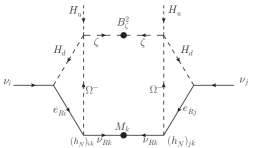
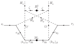
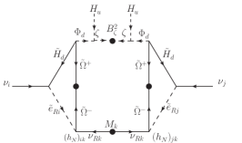
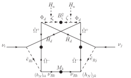
Figure 2: Three-loop diagrams which contribute to the neutrino mass matrix.

III.3 Benchmark points

We here consider the benchmark points where the neutrino oscillation data can be reproduced in addition to make 1stOPT strong as $\varphi_{c}/T_{c}\gtrsim 1$ in the $\text{SU(2)}_{H}\times Z_{2}$ model. In general, both the one-loop and the three-loop diagrams contribute to the neutrino mass generation. However, we here consider the following two limiting cases: (A) one-loop dominant case ($h_{N}^{ij}=0$), and (B) three-loop dominant case ($y_{N}^{ij}=0$). The definition of the two benchmark points are shown in Table 3. The mass of the SM-like Higgs boson is tuned to be $m_{h}=125$ GeV by choosing the parameters in the scalar top sector; i.e., SUSY breaking soft masses and left-right mixing parameter of the stops. For simplicity, we do not put any additional flavor mixing in the scalar lepton mass matrices.

Table 3: Benchmark parameter set for (A) the one-loop dominant case and (B) three-loop dominant case. For both cases, $B_{\Phi}=B_{\Omega}=A_{\zeta}=A_{\eta}=A_{\Omega^{+}}=A_{\Omega^{-}}=0$ is taken.

Case $\hat{\lambda}$ $\tan\beta$ $m_{H^{\pm}}$ $m_{\tilde{W}}$ $\mu$ $\mu_{\Phi}$ $\mu_{\Omega}$ (A) $1.8$ $15$ $350$ GeV $500$ GeV $100$ GeV $550$ GeV $-550$ GeV (B) $1.8$ $30$ $350$ GeV $500$ GeV $100$ GeV $550$ GeV $-550$ GeV

Case $\bar{m}_{\Phi_{u}}^{2}$ $\bar{m}_{\Phi_{d}}^{2}$ $\bar{m}_{\Omega^{+}}^{2}$ $\bar{m}_{\Omega^{-}}^{2}$ $\bar{m}_{\zeta}^{2}$ $\bar{m}_{\eta}^{2}$ (A) $(100\;\text{GeV})^{2}$ $(1500\;\text{GeV})^{2}$ $(1500\;\text{GeV})^{2}$ $(100\;\text{GeV})^{2}$ $(1500\;\text{GeV})^{2}$ $(2000\;\text{GeV})^{2}$ (B) $(1500\;\text{GeV})^{2}$ $(1500\;\text{GeV})^{2}$ $(1500\;\text{GeV})^{2}$ $(30\;\text{GeV})^{2}$ $(1410\;\text{GeV})^{2}$ $(30\;\text{GeV})^{2}$

Case $B_{\zeta}^{2}$ $B_{\eta}^{2}$ $m_{\zeta\eta}^{2}$ (A) $(100\;\text{GeV})^{2}$ $(100\;\text{GeV})^{2}$ $(100\;\text{GeV})^{2}$ (B) $(1400\;\text{GeV})^{2}$ $0$ $0$

Case $M_{1}$ $M_{2}$ $M_{3}$ $m_{\tilde{\nu}_{R1}}$ $m_{\tilde{\nu}_{R2}}$ $m_{\tilde{\nu}_{R3}}$ $m_{\tilde{e}_{Ri}}(i=1,2,3)$ (A) $60$ GeV $120$ GeV $180$ GeV $60$ GeV $120$ GeV $180$ GeV $5000$ GeV (B) $100$ GeV $2000$ GeV $4000$ GeV $100$ GeV $3000$ GeV $5000$ GeV $5000$ GeV

Case $(y_{N})_{ij}$ $(h_{N})_{ij}$ (A) $\begin{pmatrix}-0.439&-0.424&0.512\\ 0.226&0.218&-0.263\\ 0.272&1.36&1.36\end{pmatrix}\times 10^{-4}$ $\begin{pmatrix}0&0&0\\ 0&0&0\\ 0&0&0\\ \end{pmatrix}$ (B) $\begin{pmatrix}0&0&0\\ 0&0&0\\ 0&0&0\\ \end{pmatrix}$ $\begin{pmatrix}0.003&0&0\\ -0.0164-1.26i&-0.02424+0.0049i&-0.0022+0.00097i\\ 0.491-1.581i&0.02461+0.00537i&0.0016+0.0019i\end{pmatrix}$

We will discuss consequences of the benchmark points. First, we will show the strength of 1stOPT $\varphi_{c}/T_{c}$ and related issues in the Table 4. In order to satisfy $\varphi_{c}/T_{c}>1$ by the mechanism discussed in Ref. KSS ; KSSY , we take $\hat{\lambda}=1.8$ which leads to the cut-off scale at around $\Lambda_{H}=5$ TeV on both benchmark points. The enhancement occurs by the non-decoupling loop contributions of $Z_{2}$-odd scalars. These non-decoupling loop contributions affect the triple coupling of the SM-like Higgs boson $\lambda_{hhh}$, and loop effects of $Z_{2}$-odd charged scalars can deviate the decay branching ratio of the Higgs boson into diphoton $\text{B}(h\to\gamma\gamma)$ from the SM prediction. The ratio of $\lambda_{hhh}$ to its SM prediction and the ratio of $\text{B}(h\to\gamma\gamma)$ to its SM prediction are evaluated for each of the benchmark points as shown in Table 4, and one find 10-20% deviations for them.

Table 4: The predicted value of the cut-off scale $\Lambda_{H}$, $\varphi_{c}/T_{c}$, the ratio of the coupling constant $\lambda_{hhh}$ to its SM prediction $\lambda_{hhh}/\left.\lambda_{hhh}\right|_{\text{SM}}$, and the ratio of the branching ratio $\text{B}(h\to\gamma\gamma)$ to its SM prediction $\text{B}(h\to\gamma\gamma)/\left.\text{B}(h\to\gamma\gamma)\right|_{\text{SM}}$.

Case	$\Lambda_{H}$	$\varphi_{c}/T_{c}$	$\lambda_{hhh}/\left.\lambda_{hhh}\right|_{\text{SM}}$	$\text{B}(h\to\gamma\gamma)/\left.\text{B}(h\to\gamma\gamma)\right|_{\text{SM}}$
(A)	$5$ TeV	$1.0$	$1.18$	$0.80$
(B)	$5$ TeV	$1.2$	$1.09$	$0.89$

To see the detail of the non-decoupling effects on the condition of $\varphi_{c}/T_{c}$, $\lambda_{hhh}$ and $\text{B}(h\to\gamma\gamma)$, we show the mass spectrum of $Z_{2}$-odd particles in Table 5. In the case (A), the spectrum is very similar to the one given in Ref. KSSY . There, the charged scalar eigenstate $\Phi_{1}^{\pm}$ and $\Phi_{2}^{\pm}$ are almost from the charged scalar components of $\Omega^{-}$ and $\Phi_{u}$ respectively, and their masses are dominated by the $\hat{\lambda}^{2}v^{2}$ terms. So significant non-decoupling effects appear in 1stOPT, $\lambda_{hhh}$ and $\text{B}(h\to\gamma\gamma)$. In the neutral $Z_{2}$-odd scalar sector, there is no significant non-decoupling effects, because all the mass eigenvalues are not dominated by the Higgs vev contributions. On the other hand, in the case (B), the eigenstates $\Phi_{2}^{0}$ and $\Phi_{3}^{0}$ which are almost from the neutral components of $\eta$ give significant contributions to $\varphi_{c}/T_{c}$ and $\lambda_{hhh}$. In addition, the non-decoupling effect by $\Phi_{1}^{\pm}\sim\Omega^{-}$ contributes to $\varphi_{c}/T_{c}$, $\lambda_{hhh}$ and $\text{B}(h\to\gamma\gamma)$ as same as in the case (A).

Table 5: The mass spectrum for the $Z_{2}$-odd particles obtained from the benchmark points defined in Table 3.

Case $Z_{2}$-odd neutral bosons $\Phi_{1}^{0}$ $\Phi_{2}^{0}$ $\Phi_{3}^{0}$ $\Phi_{4}^{0}$ $\Phi_{5}^{0}$ $\Phi_{6}^{0}$ $\Phi_{7}^{0}$ $\Phi_{8}^{0}$ (A) $88.3$ GeV $88.5$ GeV $1457$ GeV $1462$ GeV $1569$ GeV $1571$ GeV $2023$ GeV $2028$ GeV (B) $126$ GeV $294$ GeV $294$ GeV $1505$ GeV $1506$ GeV $1525$ GeV $1535$ GeV $1992$ GeV

Case $Z_{2}$-odd charged bosons $\Phi_{1}^{\pm}$ $\Phi_{2}^{\pm}$ $\Phi_{3}^{\pm}$ $\Phi_{4}^{\pm}$ (A) $288$ GeV $307$ GeV $1496$ GeV $1517$ GeV (B) $271$ GeV $1459$ GeV $1506$ GeV $1574$ GeV

Case $Z_{2}$-odd neutral fermions $\tilde{\Phi}_{1}^{0}$ $\tilde{\Phi}_{2}^{0}$ $\tilde{\Phi}_{3}^{0}$ $\tilde{\Phi}_{4}^{0}$ (A) $429$ GeV $429$ GeV $721$ GeV $721$ GeV (B) $422$ GeV $422$ GeV $725$ GeV $725$ GeV

Case $Z_{2}$-odd charged fermions $\tilde{\Phi}_{1}^{\pm}$ $\tilde{\Phi}_{2}^{\pm}$ (A) S$429$ GeVS $721$ GeV (B) $422$ GeV $725$ GeV

Next, we will show the neutrino masses and mixing angles obtained on the benchmark points. In order to obtain the neutrino mass scale of order of 0.1 eV, the constants $y_{N}^{ij}$ in the case of (A) are $\mathcal{O}(10^{-4})$. On the other hand, in the case of (B), some elements of $h_{N}^{ij}$ are required to be rather large. Especially, in order to compensate the suppression by the small electron Yukawa coupling, the magnitudes of couplings $h_{N}^{1i}$ are of order one. With the coupling constant matrices $y_{N}^{ij}$ and $h_{N}^{ij}$ given in Table 3, the neutrino mass eigenvalues and the mixing angles are obtained as displayed in Table 6. These predicted values are in the allowed region which is given by the global fitting analysis of neutrino oscillation data asnufit

$$2.28<\frac{|m_{3}^{2}-m_{1}^{2}|}{10^{-3}\;\text{eV}^{2}}<2.70\;,\quad 7.0<\frac{m_{2}^{2}-m_{1}^{2}}{10^{-5}\;\text{eV}^{2}}<8.1,$$

$$0.27<\sin^{2}\theta_{12}<0.34\;,\quad 0.34<\sin^{2}\theta_{23}<0.67\;,\quad 0.016<\sin^{2}\theta_{13}<0.030\;,$$ (28)

where $m_{i}(i=1,2,3)$ are the mass eigenvalues of the neutrinos, and $\theta_{12}$, $\theta_{23}$, and $\theta_{13}$ are the mixing angles relevant to the solar neutrino mixing, atmospheric neutrino mixing and the reactor neutrino mixing respectively.

Table 6: The neutrino masses and mixing angles obtained on the benchmark points defined in Table 3.

Case	$m_{1}$	$m_{2}$	$m_{3}$	$\sin^{2}\theta_{12}$	$\sin^{2}\theta_{23}$	$|\sin\theta_{13}|$
(A)	$0.0\;\text{eV}$	$0.0087\;\text{eV}$	$0.050\;\text{eV}$	$0.31$	$0.50$	$0.14$
(B)	$0.0\;\text{eV}$	$0.0084\;\text{eV}$	$0.050\;\text{eV}$	$0.32$	$0.50$	$0.14$

The coupling constants $y_{N}^{ij}$ and $h_{N}^{ji}$ can give significant contributions to some of the lepton flavor violation processes through the RH neutrino and sneutrino mediation diagrams. The predicted values of the branching ratios $\text{B}(\mu\to e\gamma)$ and $\text{B}(\mu\to eee)$ are listed in Table 7. In the case (A), as already discussed, the coupling constants $y_{N}^{ij}$ are so small that the contribution to the $\mu\to e\gamma$ is suppressed enough to satisfy the current upper bound given by the MEG experiment $\text{B}(\mu\to e\gamma)\leq 5.7\times 10^{-13}$MEG . In addition, the branching ratio of the $\mu\to eee$ is approximately given as

$$\text{B}(\mu\to eee)\sim\frac{\alpha}{4\pi}\text{B}(\mu\to e\gamma)\;.$$ (29)

Then the experimental upper bound on the branching ratio such as $\text{B}(\mu\to eee)\leq 10^{-12}$meee is satisfied once the $\mu\to e\gamma$ is suppressed enough. In the case (B), on the other hand, large coupling constants $h_{N}^{1i}$ enhance the $\mu\to e\gamma$ process. The constraint from $\text{B}(\mu\to eee)$ is also severe in this case, even if the branching ratio $\text{B}(\mu\to e\gamma)$ is suppressed enoughaky . It is because the order one coupling constants $h_{N}^{1i}$ enhance the contributions from box diagram where the RH neutrinos and RH sneutrinos are running in the loop. The predicted values of $\text{B}(\mu\to e\gamma)$ and $\text{B}(\mu\to eee)$ on the benchmark points are shown in Table 7, and we find that they satisfy these experimental upper bounds on both benchmark points. In the case (B), since the branching ratio $\text{B}(\mu\to e\gamma)$ is predicted just below the current limit, it is expected that the $\mu\to e\gamma$ process will be observed in future experiments.

Table 7: The prediction on the branching ratios of lepton flavor violation processes $\text{B}(\mu\to e\gamma)$ and $\text{B}(\mu\to eee)$ on the benchmark points defined in Table 3.

Case	$\text{B}(\mu\to e\gamma)$	$\text{B}(\mu\to eee)$
(A)	$5.2\times 10^{-19}$	$8.1\times 10^{-21}$
(B)	$5.0\times 10^{-13}$	$8.5\times 10^{-13}$

We have found that the benchmark points defined in Table 3 can reproduce the correct values of neutrino masses and mixing angles with satisfying the constraint from lepton flavor violations and with keeping strong enough 1stOPT for electroweak baryogenesis.

III.4 Collider signatures

In this paper, we do not perform any complete analysis of specific collider signals. We here give some comments, and detailed analysis of collider signatures in our model will be discussed elsewhere.

III.4.1 Precise measurements of the Higgs couplings

As shown in Ref. KSSY , in the parameter region where 1stOPT becomes strong enough for successful electroweak baryogenesis, the non-decoupling effect gives significant contributions to Higgs couplings such as the $hhh$ coupling and the $h\gamma\gamma$ coupling. The direction of deviations for these coupling constants are related to each other. Both couplings can deviate as large as $20$% from the SM predictions, which can be tested by future collider experiments. At the LHC, the branching ratio of Higgs to diphoton process will be measured at about 20% accuracy, but the measurement of triple Higgs boson coupling is very challenging. At the HL-LHC with the luminosity of 3000 $\text{fb}^{-1}$, $\text{B}(h\to\gamma\gamma)$ will be measured with 10% accuracyHLLHC . The triple Higgs boson coupling can be measured at the HL-LHC and much better at the ILC. It is expected that the $hhh$ coupling can be measured with the accuracy of about 20 % or better at the ILC with $\sqrt{s}=1$ TeV with 2 ab^-1TDRILC .

III.4.2 Direct search of the extra particles

There are many extra fields which can provide collider signals in our model. The $Z_{2}$-even sector of our model is essentially same as the nMSSM. Therefore we can expect that the collider signals relevant to the $Z_{2}$-even particles are same as them in the nMSSM which are studied in the literaturecollidernMSSM .

Our model is characterized by the $Z_{2}$-odd sector, so that the collider signals in this sector are very important. In the case (A) of our benchmark points, inert doublet-like scalars are light. Collider signatures of the inert doublet scalars have been studied in the literatureColliderID ; AokiKanemura ; AKYok . The inert doublet scalars are color singlet particles, then it is not easy to discover them at the LHC. Even though they can be fortunately discovered at the LHC, precise determination of their masses and quantum numbers are challengingColliderID . On the other hand, the ILC is a very powerful tool to study such non-colored inert doublet particles. At the ILC, the mass of charged inert scalar can be measured in a few GeV accuracy, and the mass of neutral inert scalar can be measured in better than 2 GeV accuracyAKYok .

In the case (B), the $Z_{2}$-odd singlet-like charged particle is required to be light. As discussed in Ref. aks2 , such the light singlet-like charged particle can be studied at the ILC via the pair production such as $e^{+}e^{-}\to\varphi_{1}^{+}\varphi_{1}^{-}$. Furthermore, due to the interaction of $N_{i}^{c}E_{j}^{c}\Omega^{-}$, the production process such as $e^{-}e^{-}\to\varphi_{1}^{-}\varphi_{1}^{-}$ is possible. This process will be a strong evidence of three-loop neutrino mass generation mechanismAokiKanemura . The process can be detected at the $e^{-}e^{-}$ collision option of the ILC or the CLICaks2 ; AokiKanemura .

In addition, the SUSY extended Higgs sector of this model includes several color singlet SUSY partner fermions of the extra scalars. If such SUSY partner particles are discovered, it discriminates our model from non-SUSY models with radiative seesaw scenarios.

III.5 Discussions

III.5.1 Evaluation of the baryon asymmetry of the Universe

For baryogenesis, we focus on the strength of 1stOPT which gives a necessary condition for successful electroweak baryogenesis, and we have not numerically evaluated the prediction on the BAU in our scenario. In order to complete the numerical evaluation of the BAU, we should also take care of the CP phases. Since it is known that the CP violation in the SM is too small for getting the enough large BAUCPinSM , extra CP phases are also required in addition to the mechanism to enhance 1stOPT. In SUSY models, new sources of the CP violation which can contribute to the generation of the BAU can be introducedCPinSUSY . In the literatureSUSYEWBG , numerical evaluation of the BAU due to the electroweak baryogenesis in the MSSM is discussed. In principle, we can introduce the CP phases to the model in the similar ways as the works mentioned above. We then expect to obtain sufficient amount of BAU, once the strong enough 1stOPT is realized.

III.5.2 Dark matter

This model includes an unbroken $Z_{2}$ parity, which provides DM candidates. Since the $Z_{2}$-odd extra fields except for the RH neutrino have quite strong coupling with the Higgs bosons, they conflict with the bounds from direct detection experiments of the DM. We choose the both benchmark points in such a way that the lightest $Z_{2}$-odd particle is the RH neutrino and/or the RH sneutrino. If the $R$ parity is also imposed, the lightest SUSY particle also qualifies as the DM candidate. It leads to a rich possibility of the multi-component DM scenariomultiDM . In this paper we do not specify the scenario of DM. Detailed analysis of the relic abundance and the direct detection constraints are performed elsewhere.

III.5.3 Mediation mechanism of the SUSY breaking

Due to the non-renormalization theorem, the neutrino masses are not generated supersymmetric; i.e., soft SUSY breaking terms are necessary for loop induced neutrino mass models. In our model, SUSY breaking terms in the last line of Eq. (20) are essential. These terms are not forbidden by the gauge symmetry, but no relevant terms are in the superpotential given in Eq. (19). It may suggest a specific mediation mechanism for the SUSY breaking. It is a quite interesting point that the neutrino mass generation is a key to explore the mediation mechanism of SUSY breaking in our model.

IV Conclusions

We have considered a model based on the SUSY gauge theory with $N_{c}=2$ and $N_{f}=3$ with an additional exact $Z_{2}$ symmetry. By adding $Z_{2}$-odd RH neutrinos to the model, we have proposed a concrete model which can be a fundamental theory of a low energy effective theory with radiative seesaw scenarios and with strong 1stOPT. We have shown that radiative seesaw scenarios can be realized in our model and there can be two types of contributions to the neutrino mass matrix; i.e., by one-loop diagrams and also by three-loop diagrams. These contributions correspond to the SUSY versions of the Ma model and the AKS model, respectively. We have also found out the benchmark point for each contributions, where the neutrino oscillation data are correctly reproduced with satisfying the condition of strong 1stOPT and with satisfying the current experimental constraints. Our model is a candidate of the fundamental theory whose low energy effective theory provides solutions to three serious problems in the SM; i.e., neutrino mass, DM and baryogenesis by physics at the TeV scale. Our model can be tested at current and future collider experiments.

Appendix A Mass matrices and mixing matrices for extra fields

Here we will list the mass terms of $Z_{2}$-odd particles which are obtained from the superpotential given by Eq. (19) and the soft SUSY breaking terms given by Eq. (20), and we will define the mixing matrices.

The mass terms for the $Z_{2}$ odd neutral scalars are given by

$$\mathcal{L}=-\begin{pmatrix}\Phi_{u}^{\text{even}}&\zeta^{\text{even}}&\Phi_{d}^{\text{even}}&\eta^{\text{even}}&\Phi_{u}^{\text{odd}}&\zeta^{\text{odd}}&\Phi_{d}^{\text{odd}}&\eta^{\text{odd}}\end{pmatrix}M_{0}^{2}\begin{pmatrix}\Phi_{u}^{\text{even}}\\ \zeta^{\text{even}}\\ \Phi_{d}^{\text{even}}\\ \eta^{\text{even}}\\ \Phi_{u}^{\text{odd}}\\ \zeta^{\text{odd}}\\ \Phi_{d}^{\text{odd}}\\ \eta^{\text{odd}}\end{pmatrix}\;,$$ (30)

where the superscript ”even” and ”odd” denote the CP-even neutral scalar component and CP-odd neutral scalar component respectively. The $8\times 8$ mass matrix $M_{0}^{2}$ can be written as

$$M_{0}^{2}=\begin{pmatrix}M_{\varphi\varphi}^{2}&M_{\varphi\chi}^{2}\\ (M_{\varphi\chi}^{2})^{T}&M_{\chi\chi}^{2}\end{pmatrix}\;,$$ (31)

where the three $4\times 4$ matrices are defined as

$$M_{\varphi\varphi}^{2}=\mathrm{Re}M_{\phi^{0}}^{2}+\begin{pmatrix}0&0&0&0\\ 0&\mathrm{Re}(B_{\zeta}^{2})&0&\mathrm{Re}(m_{\zeta\eta}^{2})\\ 0&0&0&0\\ 0&\mathrm{Re}(m_{\zeta\eta}^{2})&0&\mathrm{Re}(B_{\eta}^{2})\\ \end{pmatrix}\;,$$ (32)

$$M_{\chi\chi}^{2}=\mathrm{Re}M_{\phi^{0}}^{2}+\begin{pmatrix}0&0&0&0\\ 0&-\mathrm{Re}(B_{\zeta}^{2})&0&\mathrm{Re}(m_{\zeta\eta}^{2})\\ 0&0&0&0\\ 0&\mathrm{Re}(m_{\zeta\eta}^{2})&0&-\mathrm{Re}(B_{\eta}^{2})\\ \end{pmatrix}\;,$$ (33)

$$M_{\varphi\chi}^{2}=-\mathrm{Im}M_{\phi^{0}}^{2}+\begin{pmatrix}0&0&0&0\\ 0&-\mathrm{Im}(B_{\zeta}^{2})&0&-\mathrm{Im}(m_{\zeta\eta}^{2})\\ 0&0&0&0\\ 0&\mathrm{Im}(m_{\zeta\eta}^{2})&0&-\mathrm{Im}(B_{\eta}^{2})\\ \end{pmatrix}\;,$$ (34)

and

$$M_{\varphi^{0}}^{2}=\begin{pmatrix}\bar{m}_{\Phi_{u}}^{2}+\hat{\lambda}^{2}\frac{v_{d}^{2}}{2}+D_{\Phi^{0}}&\hat{\lambda}^{*}\mu\frac{v_{u}}{\sqrt{2}}+A_{\zeta}^{*}\frac{v_{d}}{\sqrt{2}}&-B_{\Phi}^{*}\mu_{\Phi}^{*}&\hat{\lambda}^{*}\mu_{\Omega}\frac{v_{d}}{\sqrt{2}}-\hat{\lambda}\mu_{\Phi}^{*}\frac{v_{u}}{\sqrt{2}}\\ \hat{\lambda}\mu^{*}\frac{v_{u}}{\sqrt{2}}+A_{\zeta}\frac{v_{d}}{\sqrt{2}}&\bar{m}_{\zeta}^{2}+\hat{\lambda}^{2}\frac{v_{d}^{2}}{2}&\hat{\lambda}\mu_{\Phi}^{*}\frac{v_{d}}{2}-\hat{\lambda}^{*}\mu_{\Omega}\frac{v_{u}}{\sqrt{2}}&B_{\Omega}\mu_{\Omega}\\ -B_{\Phi}\mu_{\Phi}&\hat{\lambda}^{*}\mu_{\Phi}\frac{v_{d}}{\sqrt{2}}-\hat{\lambda}\mu_{\Omega}^{*}\frac{v_{u}}{\sqrt{2}}&\bar{m}_{\Phi_{d}}^{2}+\hat{\lambda}^{2}\frac{v_{u}^{2}}{2}-D_{\Phi^{0}}&-\hat{\lambda}\mu^{*}\frac{v_{d}}{\sqrt{2}}-A_{\eta}\frac{v_{u}}{\sqrt{2}}\\ \hat{\lambda}\mu_{\Omega}^{*}\frac{v_{d}}{\sqrt{2}}-\hat{\lambda}^{*}\mu_{\Phi}\frac{v_{u}}{\sqrt{2}}&B_{\Omega}^{*}\mu_{\Omega}^{*}&-\hat{\lambda}^{*}\mu\frac{v_{d}}{\sqrt{2}}-A_{\eta}^{*}\frac{v_{u}}{\sqrt{2}}&\bar{m}_{\eta}^{2}+\hat{\lambda}^{2}\frac{v_{u}^{2}}{2}\\ \end{pmatrix}\;.$$ (35)

The matrix $M_{0}^{2}$ is diagonalized by a real orthogonal matrix $O_{0}$ as

$$O_{0}^{T}M_{0}^{2}O_{0}=\begin{pmatrix}m_{\Phi_{1}^{0}}^{2}&0&0&0&0&0&0&0\\ 0&m_{\Phi_{2}^{0}}^{2}&0&0&0&0&0&0\\ 0&0&m_{\Phi_{3}^{0}}^{2}&0&0&0&0&0\\ 0&0&0&m_{\Phi_{4}^{0}}^{2}&0&0&0&0\\ 0&0&0&0&m_{\Phi_{5}^{0}}^{2}&0&0&0\\ 0&0&0&0&0&m_{\Phi_{6}^{0}}^{2}&0&0\\ 0&0&0&0&0&0&m_{\Phi_{7}^{0}}^{2}&0\\ 0&0&0&0&0&0&0&m_{\Phi_{8}^{0}}^{2}\end{pmatrix}\;.$$ (36)

The mass terms for $Z_{2}$-odd neutral fermions are written as

$$\mathcal{L}=-\frac{1}{2}\begin{pmatrix}\tilde{\Phi}_{u}^{0}&\tilde{\zeta}^{0}&\tilde{\Phi}_{d}^{0}&\tilde{\eta}^{0}\end{pmatrix}\tilde{M}_{0}\begin{pmatrix}\tilde{\Phi}_{u}^{0}\\ \tilde{\zeta}^{0}\\ \tilde{\Phi}_{d}^{0}\\ \tilde{\eta}^{0}\end{pmatrix}\;,$$ (37)

where the mass matrix is given by

$$\tilde{M}_{0}=\begin{pmatrix}0&\hat{\lambda}\frac{v_{d}}{\sqrt{2}}&\mu_{\Phi}&0\\ \hat{\lambda}\frac{v_{d}}{\sqrt{2}}&0&0&\mu_{\Omega}\\ \mu_{\Phi}&0&0&-\hat{\lambda}\frac{v_{u}}{\sqrt{2}}\\ 0&-\hat{\lambda}\frac{v_{u}}{\sqrt{2}}&\mu_{\Omega}&0\end{pmatrix}\;.$$ (38)

The mass matrix $\tilde{M}_{0}$ can be diagonalized by a unitary matrix $\tilde{U}_{0}$ as

$$\tilde{U}_{0}^{T}\tilde{M}_{0}\tilde{U}_{0}=\begin{pmatrix}m_{\tilde{\Phi}_{1}^{0}}&0&0&0\\ 0&m_{\tilde{\Phi}_{2}^{0}}&0&0\\ 0&0&m_{\tilde{\Phi}_{3}^{0}}&0\\ 0&0&0&m_{\tilde{\Phi}_{4}^{0}}\end{pmatrix}\;,$$ (39)

and one can obtain the real and positive mass eigenvalues $m_{\tilde{\Phi}_{i}}$.

The mass terms for the $Z_{2}$-odd charged scalars are given by

$$\mathcal{L}=-\begin{pmatrix}(\Phi_{u}^{+})^{*}&(\Omega^{+})^{*}&\Phi_{d}^{-}&\Omega^{-}\end{pmatrix}M_{\pm}^{2}\begin{pmatrix}\Phi_{u}^{+}\\ \Omega^{+}\\ (\Phi_{d}^{-})^{*}\\ (\Omega^{-})^{*}\\ \end{pmatrix}\;,$$ (40)

with the mass matrix being

$$M_{\pm}^{2}=\begin{pmatrix}\bar{m}_{\Phi_{u}}^{2}+\hat{\lambda}^{2}\frac{v_{u}^{2}}{2}+D_{\Phi\pm}&\hat{\lambda}\mu_{\Phi}^{*}\frac{v_{d}}{\sqrt{2}}-\hat{\lambda}^{*}\mu_{\Omega}\frac{v_{u}}{\sqrt{2}}&B^{*}\mu_{\Phi}^{*}&\hat{\lambda}^{*}\mu\frac{v_{d}}{\sqrt{2}}-A_{\Omega^{-}}^{*}\frac{v_{u}}{\sqrt{2}}\\ \hat{\lambda}^{*}\mu_{\Phi}\frac{v_{d}}{\sqrt{2}}-\hat{\lambda}\mu_{\Omega}^{*}\frac{v_{u}}{\sqrt{2}}&\bar{m}_{\Omega^{+}}^{2}+\hat{\lambda}^{2}\frac{v_{d}^{2}}{2}+D_{\Omega\pm}&-\hat{\lambda}^{*}\mu\frac{v_{u}}{\sqrt{2}}+A_{\Omega^{+}}^{*}\frac{v_{d}}{\sqrt{2}}&B^{*}\mu_{\Omega}^{*}\\ B\mu_{\Phi}&-\hat{\lambda}\mu^{*}\frac{v_{u}}{\sqrt{2}}+A_{\Omega^{+}}\frac{v_{d}}{\sqrt{2}}&\bar{m}_{\Phi_{d}}^{2}+\hat{\lambda}^{2}\frac{v_{d}^{2}}{2}-D_{\Phi\pm}&\hat{\lambda}\mu_{\Omega}^{*}\frac{v_{d}}{\sqrt{2}}-\hat{\lambda}^{*}\mu_{\Phi}\frac{v_{u}}{\sqrt{2}}\\ \hat{\lambda}\mu^{*}\frac{v_{d}}{\sqrt{2}}-A_{\Omega^{-}}\frac{v_{u}}{\sqrt{2}}&B\mu_{\Omega}&\hat{\lambda}^{*}\mu_{\Omega}\frac{v_{d}}{\sqrt{2}}-\hat{\lambda}\mu_{\Phi}^{*}\frac{v_{u}}{\sqrt{2}}&\bar{m}_{\Omega^{-}}^{2}+\hat{\lambda}^{2}\frac{v_{u}^{2}}{2}-D_{\Omega\pm}\end{pmatrix}\;.$$ (41)

The mass matrix $M_{\pm}^{2}$ can be diagonalized by a unitary matrix $U_{+}$ as

$$U_{+}^{\dagger}M_{\pm}^{2}{U}_{+}=\begin{pmatrix}m_{{\Phi}_{1}^{\pm}}^{2}&0&0&0\\ 0&m_{{\Phi}_{2}^{\pm}}^{2}&0&0\\ 0&0&m_{{\Phi}_{3}^{\pm}}^{2}&0\\ 0&0&0&m_{{\Phi}_{4}^{\pm}}^{2}\end{pmatrix}\;.$$ (42)

The mass terms of the $Z_{2}$-odd charged fermions are written as

$$\mathcal{L}=-\begin{pmatrix}\tilde{\Phi}_{u}^{+}&\tilde{\Omega}^{+}\end{pmatrix}\tilde{M}_{\pm}\begin{pmatrix}\tilde{\Phi}_{d}^{-}\\ \tilde{\Omega}^{-}\end{pmatrix}\;,$$ (43)

where the mass matrix is given by

$$\tilde{M}_{\pm}=\begin{pmatrix}-\mu_{\Phi}&\hat{\lambda}\frac{v_{u}}{\sqrt{2}}\\ -\hat{\lambda}\frac{v_{d}}{\sqrt{2}}&-\mu_{\Omega}\end{pmatrix}\;.$$ (44)

The mass matrix $\tilde{M}_{\pm}$ is diagonalized by two unitary matrices $U_{L}$ and $U_{R}$ as

$$U_{R}^{\dagger}\tilde{M}_{\pm}U_{L}=\begin{pmatrix}m_{\tilde{\Phi}^{\pm}_{1}}&0\\ 0&m_{\tilde{\Phi}^{\pm}_{2}}\end{pmatrix}\;,$$ (45)

where $m_{\tilde{\Phi}_{i}^{\pm}}$ are the real and positive mass eigenvalues.

References

• (1) G. Aad et al. [ATLAS Collaboration], Phys. Lett. B 716 (2012) 1; S. Chatrchyan et al. [CMS Collaboration], Phys. Lett. B 716 (2012) 30.
• (2) [ATLAS Collaboration], ATLAS-CONF-2013-034; [CMS Collaboration], CMS-PAS-HIG-12-045.
• (3) A. Zee, Phys. Lett. B 93 (1980) 389 [Erratum-ibid. B 95 (1980) 461].
• (4) A. Zee, Nucl. Phys. B 264 (1986) 99; K. S. Babu, Phys. Lett. B 203 (1988) 132.
• (5) E. Ma, Phys. Rev. D 73 (2006) 077301.
• (6) L. M. Krauss, S. Nasri and M. Trodden, Phys. Rev. D 67 (2003) 085002.
• (7) M. Aoki, S. Kanemura and O. Seto, Phys. Rev. Lett.  102 (2009) 051805.
• (8) M. Aoki, S. Kanemura and O. Seto, Phys. Rev. D 80 (2009) 033007.
• (9) V. A. Kuzmin, V. A. Rubakov and M. E. Shaposhnikov, Phys. Lett. B 155 (1985) 36; A. G. Cohen, D. B. Kaplan and A. E. Nelson, Ann. Rev. Nucl. Part. Sci.  43 (1993) 27; M. Quiros, Helv. Phys. Acta 67 (1994) 451; V. A. Rubakov and M. E. Shaposhnikov, Usp. Fiz. Nauk 166 (1996) 493 [Phys. Usp.  39 (1996) 461]; K. Funakubo, Prog. Theor. Phys.  96 (1996) 475; M. Trodden, Rev. Mod. Phys.  71 (1999) 1463; W. Bernreuther, Lect. Notes Phys.  591 (2002) 237; J. M. Cline, hep-ph/0609145; D. E. Morrissey and M. J. Ramsey-Musolf, New J. Phys.  14 (2012) 125003.
• (10) M. Aoki, S. Kanemura and K. Yagyu, Phys. Rev. D 83 (2011) 075016.
• (11) R. Harnik, G. D. Kribs, D. T. Larson and H. Murayama, Phys. Rev. D 70 (2004) 015002.
• (12) S. Chang, C. Kilic and R. Mahbubani, Phys. Rev. D 71 (2005) 015003; A. Delgado and T. M. P. Tait, JHEP 0507 (2005) 023.
• (13) K. A. Intriligator and N. Seiberg, Nucl. Phys. Proc. Suppl.  45BC (1996) 1.
• (14) C. Panagiotakopoulos and K. Tamvakis, Phys. Lett. B 446 (1999) 224; C. Panagiotakopoulos and K. Tamvakis, Phys. Lett. B 469 (1999) 145; C. Panagiotakopoulos and A. Pilaftsis, Phys. Rev. D 63 (2001) 055003; A. Dedes, C. Hugonie, S. Moretti and K. Tamvakis, Phys. Rev. D 63 (2001) 055009.
• (15) C. Liu, Phys. Rev. D 61 (2000) 115001; M. A. Luty, J. Terning and A. K. Grant, Phys. Rev. D 63 (2001) 075001; H. Murayama, hep-ph/0307293; T. Abe and R. Kitano, Phys. Rev. D 88 (2013) 015019.
• (16) S. Kanemura, T. Shindou and T. Yamada, Phys. Rev. D 86 (2012) 055023.
• (17) S. Kanemura, Y. Okada and E. Senaha, Phys. Lett. B 606 (2005) 361.
• (18) C. Grojean, G. Servant and J. D. Wells, Phys. Rev. D 71 (2005) 036001.
• (19) S. Kanemura, E. Senaha and T. Shindou, Phys. Lett. B 706 (2011) 40.
• (20) S. Kanemura, E. Senaha, T. Shindou and T. Yamada, JHEP 1305 (2013) 066.
• (21) H. Georgi, A. Manohar and G. W. Moore, Phys. Lett. B 149 (1984) 234; H. Georgi and L. Randall, Nucl. Phys. B 276 (1986) 241; M. A. Luty, Phys. Rev. D 57 (1998) 1531; A. G. Cohen, D. B. Kaplan and A. E. Nelson, Phys. Lett. B 412 (1997) 301.
• (22) F. D’Eramo and J. Thaler, JHEP 1006 (2010) 109; G. Belanger and J. -C. Park, JCAP 1203 (2012) 038; G. Belanger, K. Kannike, A. Pukhov and M. Raidal, JCAP 1204 (2012) 010; M. Aoki, M. Duerr, J. Kubo and H. Takano, Phys. Rev. D 86 (2012) 076015; M. Aoki, J. Kubo and H. Takano, Phys. Rev. D 87 (2013) 116001.
• (23) S. Kanemura, N. Machida, T. Shindou, and T. Yamada, work in progress.
• (24) G. L. Fogli, E. Lisi, A. Marrone, D. Montanino, A. Palazzo and A. M. Rotunno, Phys. Rev. D 86 (2012) 013012; M. C. Gonzalez-Garcia, M. Maltoni, J. Salvado and T. Schwetz, JHEP 1212 (2012) 123.
• (25) J. Adam et al. [MEG Collaboration] Phys. Rev. Lett. 110 (2013) 201801.
• (26) U. Bellgardt et al. [SINDRUM Collaboration], Nucl. Phys. B 299 (1988) 1.
• (27) ATLAS Collaboration, ATL-PHYS-PUB-2012-001; ATL-PHYS-PUB-2012-004.
• (28) H. Baer, T. Barklow, K. Fujii, Y. Gao, A. Hoang, S. Kanemura, J. List and H. E. Logan et al., arXiv:1306.6352 [hep-ph].
• (29) C. Balazs, M. S. Carena, A. Freitas and C. E. M. Wagner, JHEP 0706 (2007) 066; J. Cao, H. E. Logan and J. M. Yang, Phys. Rev. D 79 (2009) 091701.
• (30) R. Barbieri, L. J. Hall and V. S. Rychkov, Phys. Rev. D 74 (2006) 015007; A. Goudelis, B. Herrmann and O. Stal, arXiv:1303.3010 [hep-ph]; Q. -H. Cao, E. Ma and G. Rajasekaran, Phys. Rev. D 76 (2007) 095011; E. Lundstrom, M. Gustafsson and J. Edsjo, Phys. Rev. D 79 (2009) 035013; E. Dolle, X. Miao, S. Su and B. Thomas, Phys. Rev. D 81 (2010) 035003 X. Miao, S. Su and B. Thomas, Phys. Rev. D 82 (2010) 035009; M. Gustafsson, S. Rydbeck, L. Lopez-Honorez and E. Lundstrom, Phys. Rev. D 86 (2012) 075019.
• (31) M. Aoki and S. Kanemura, Phys. Lett. B 689 (2010) 28.
• (32) M. Aoki, S. Kanemura and H. Yokoya, Phys. Lett. B 725 (2013) 302.
• (33) M. B. Gavela, M. Lozano, J. Orloff and O. Pene, Nucl. Phys. B 430 (1994) 345; M. B. Gavela, P. Hernandez, J. Orloff, O. Pene and C. Quimbay, Nucl. Phys. B 430 (1994) 382; P. Huet and E. Sather, Phys. Rev. D 51 (1995) 379.
• (34) M. Dine, P. Huet, R. L. Singleton, Jr and L. Susskind, Phys. Lett. B 257 (1991) 351; A. G. Cohen and A. E. Nelson, Phys. Lett. B 297 (1992) 111.
• (35) P. Huet and A. E. Nelson, Phys. Rev. D 53 (1996) 4578; P. Huet and A. E. Nelson, Phys. Rev. D 53 (1996) 4578; M. S. Carena, M. Quiros, A. Riotto, I. Vilja and C. E. M. Wagner, Nucl. Phys. B 503 (1997) 387; J. M. Cline, M. Joyce and K. Kainulainen, Phys. Lett. B 417 (1998) 79 [Erratum-ibid. B 448 (1999) 321]; A. Riotto, Nucl. Phys. B 518 (1998) 339; A. Riotto, Phys. Rev. D 58 (1998) 095009; M. Trodden, Rev. Mod. Phys.  71 (1999) 1463; J. M. Cline and K. Kainulainen, Phys. Rev. Lett.  85 (2000) 5519; J. M. Cline, M. Joyce and K. Kainulainen, JHEP 0007 (2000) 018; M. S. Carena, J. M. Moreno, M. Quiros, M. Seco and C. E. M. Wagner, Nucl. Phys. B 599 (2001) 158; M. S. Carena, M. Quiros, M. Seco and C. E. M. Wagner, Nucl. Phys. B 650 (2003) 24.