Cold Bose Atoms Around the Crossing of Quantum Waveguides.

Abstract

We show that massive low energy particles traversing a branching zone or a crossing of quantum waveguides may experience a non standard trapping force that cannot be derived from a potential. For interacting cold Bose atoms we report on the formation of a localised Hartree ground state for three prototype waveguide geometries with broken translational symmetry: a cranked $L$-shaped waveguide $\mathcal{L}$, a $T$-shaped waveguide $\mathcal{T}$ , and the crossing $\mathcal{C}$ of two quantum waveguides. The phenomenon is kinetic energy driven and cannot be described within the Thomas-Fermi approximation. Depending on the ratio $\kappa^{\left(\Gamma\right)}$ of joining lateral tube diameters of the respective waveguides $\Gamma\in\left\{\mathcal{C},\mathcal{L},\mathcal{T}\right\}$ delocalisation commences when the particle number $N$ approaches a critical value $N_{c}^{\left(\Gamma\right)}$. For the case of a binary mixture of two different Bose atom species $A$ and $B$ we observe non standard trapping of both atom species for subcritical particle numbers. A sudden demixing quantum transition takes place as the total particle number $N=N_{A}+N_{B}$ is increased at fixed mixing ratio $N_{A}/N_{B}$. Depending on the mass ratio $m_{A}/m_{B}$ the heavier atom species delocalises first for a wide range of interaction parameters. The numerical calculations are based on a splitting scheme involving an analytic approximation to the short time asymptotics of the imaginary time quantum propagator of a single particle obeying to Dirichlet boundary conditions at the walls inside the respective waveguides.

PACS numbers

03.75.Hh, 67.85.-d, 67.85.Hj, 05.30.Jp, 03.75.Be, 42.25.-p, 03.75.-b

I Introduction

Elementary quantum mechanics predicts, that the dispersion relation $E_{p}=\frac{p^{2}}{2m}$ of a massive particle in free space is modified, when the particle is moving slowly inside a hollow micron-sized capillary tube with a transverse size $w$ comparable to the thermal de Broglie wavelength $\lambda_{th}$ of that particle. This is because boundary conditions at the hard walls of such a tube eliminate an infinite number of solutions to the Schrödinger equation in free space, and the ones remaining are the guided matter waves. In full analogy to $TE$- and $TM$- modes used for transmitting electromagnetic signals along waveguides, also matter waves propagating along the axis of a hollow tube sustain a discrete set of guided modes. For example, guided waves of ultracold neutrons have been observed in metallic thin film waveguides Feng ,Pogossian .

More recently guided matter wave experiments with cold atoms, using various optical techniques for atom confinement in hollow-core dielectric fibers, have been carried out successfully by several groups Renn I , Ito et al , Mueller I , Christensen I , vorrath , Pechkis . Also the trapping and guiding of atoms in the evanescent light field surrounding a thin subwavelength-diameter fiber Barnett et al , K+B+H has been observed recently Nayak et al , Vetsch et al . A new type of atomic-cladding waveguide with a dimension on the sub-micro-meter scale Stern opens further new possibilities for experiments with guided atoms. Also cylindrically blue-tuned dark hollow light beams are capable to transport atoms along their dark core Schiffer et al , jc0 .

With the emergence of guided matter wave experiments the question then arises, what happens if ultra cold particles were carried along curved waveguides, or were transported across the branching zone or the crossing of two waveguides.

Theoretical studies of the motion of particles confined in branching planar stripes srw or curved quantum wires have been the subject of intense theoretical research already for many years ez0 ,ez1 ,D+E , Br+Es , Avishai , sad , Nazarov I , Dauge . It is well known, that inside an infinitely extended straight waveguide the propagation of a stationary mode along the tube axis is enabled only if the energy $E$ of that mode is above a certain excitation threshold $\varepsilon_{xt}>0$, the precise value of $\varepsilon_{xt}$ depending on the geometric shape of the cross section of that waveguide. However, as was shown by Goldstone and Jaffe gj0 , even a slight deviation from being exactly straight may then give rise to the formation of localised states, i.e. there exist stationary eigenstates of the kinetic energy Hamiltonian with an eigenvalue $E_{0}$ below the excitation threshold $\varepsilon_{xt}$. Localised states also exist at a crossing of two waveguides srw . Since such bound states originate from effects of interference, they are absent within a classical point mechanics approach. The trapping force confining the particles by this mechanism is non standard and cannot be derived from a potential. It is based on the rapid variation of kinetic energy of a quantum particle that traverses a crossing or branching region of otherwise translational invariant waveguides.

A long hollow tube with hard walls and constant cross-section along the tube axis will be referred to as a quantum waveguide (QW), if the thermal de Broglie wavelength $\lambda_{th}$ of a particle moving inside is comparable to the transversal size $w$ of the tubes forming that QW. We consider in the following three prototypes of QW geometries with broken translational symmetry. The first consists of two intersecting orthogonal tubes with rectangular cross-section, comprising four arms $\mathcal{A}_{1}$,$...$,$\mathcal{A}_{4}$ and a central zone $\mathcal{A}_{0}$, altogether forming an open three-dimensional waveguide geometry in the guise of a swiss cross $\mathcal{C}$ with boundary surface $\partial\mathcal{C}$ as displayed schematically in Fig.1. The second, in the following referred to as $\mathcal{L}$, consists of a cranked tube that is $L$-shaped, the third, in the following referred to as $\mathcal{T}$ , consists of a $T$-shaped branching joining three tubes, see Fig.1.

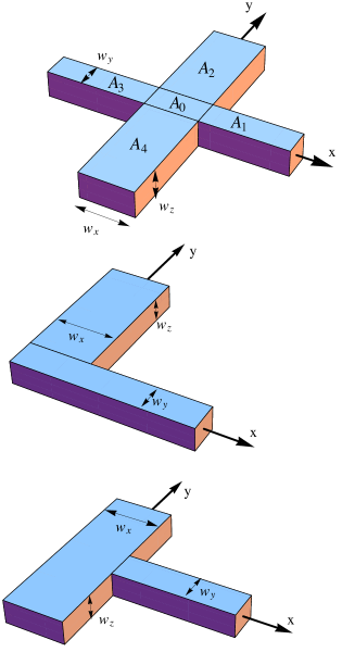
Figure 1: Three prototypes of waveguides with broken translational symmetry. 1) Cross shaped waveguide $\mathcal{C}$ as generated by two intersecting tubes of rectangular cross-section. 2) $L$-shaped waveguide $\mathcal{L}$. 3) $T$-shaped waveguide $\mathcal{T}$ . The respective tube diameters are denoted as $w_{x}$, $w_{y}$, and $w_{z}$.

It appears then natural to ask if a QW with a bulge or bent like $\mathcal{L}$, or with a branching like $\mathcal{T}$ , or a crossing of two waveguides like $\mathcal{C}$, could be used as a particle trap for ultra cold particles. With a repulsive interaction present, the number of Bose particles that may occupy these bound states is limited to a critical maximum value $N_{c}$ lp0 .

In the ensuing discussion we investigate localised ground states of interacting cold Bose atoms inside the waveguides $\Gamma\in\left\{\mathcal{C},\mathcal{L},\mathcal{T}\right\}$ for various cross section areas and various particle numbers $N$. We determine the critical number $N_{c}^{\left(\Gamma\right)}$ of particles that can be trapped around the respective crossing or branching regions. We show for cold Bose atoms confined in such non classical traps that their kinetic energy is not negligible (even for huge particle numbers), and that the Thomas-Fermi approximation does not apply, a characteristic difference to the well known BEC-atom traps with a parabolic potential.

Restricting to a mean field description of ultracold interacting Bose atoms with mass $m$ we are interested in the Hartree ground state

$$\Psi_{G}^{\left(\Gamma\right)}(\mathbf{r}_{1},\mathbf{r}_{2},...,\mathbf{r}_{N})=\psi^{\left(\Gamma\right)}(\mathbf{r}_{1})\psi^{\left(\Gamma\right)}(\mathbf{r}_{2})\cdot\cdot\psi^{\left(\Gamma\right)}(\mathbf{r}_{N})$$ (1)

that forms inside the respective QW’s subject to the constraint

$$\int_{\Gamma}d^{3}r|\psi^{\left(\Gamma\right)}(\mathbf{r})|^{2}=1$$ (2)

The task is then to find the optimal one-particle orbital $\psi^{\left(\Gamma\right)}(\mathbf{r})$ that minimizes the energy of the interacting Bose gas subject to a normalisation constraint ensuring conservation of particle number $N$. Introducing a Lagrange parameter $\mu_{N}^{\left(\Gamma\right)}$ for this constraint the optimal orbital $\psi^{\left(\Gamma\right)}(\mathbf{r})$ is then found solving the Gross-Pitaevskii equation

$$\left(-\frac{\hbar^{2}}{2m}\nabla^{2}+V_{T}^{\left(\Gamma\right)}(\mathbf{r})+\left(N-1\right)\frac{4\pi\hbar^{2}a_{s}}{m}\ |\psi^{\left(\Gamma\right)}(\mathbf{r})|^{2}\right)\psi^{\left(\Gamma\right)}(\mathbf{r})=\mu_{N}^{\left(\Gamma\right)}\psi^{\left(\Gamma\right)}(\mathbf{r})$$ (3)

Here, $a_{S}$ denotes the $s$-wave scattering length characterizing the repulsive two-particle contact interaction. In order that such a mean field description applies all tube size parameters $w_{a}^{\left(\Gamma\right)}$should be large compared to $a_{s}$. For hollow tubes $\Gamma\in\left\{\mathcal{C},\mathcal{L},\mathcal{T}\right\}$ with hard walls $\partial\Gamma$ the effect of the trap potential

$$V_{T}^{\left(\Gamma\right)}(\mathbf{r})=\left\{\begin{array}[]{c}0\text{ for }\mathbf{r}\in\Gamma\\ \infty\text{ for }\mathbf{r}\in\Gamma\end{array}\right.$$ (4)

will be taken into account in the following posing Dirichlet boundary value conditions at these walls:

$$\psi^{\left(\Gamma\right)}(\mathbf{r})|_{\mathbf{r}\in\partial\Gamma}=0$$ (5)

In the numerical calculations we use scaled units: $r_{a}\rightarrow r_{a}/L$, $\,\mu_{N}^{\left(\Gamma\right)}\rightarrow\mu_{N}^{\left(\Gamma\right)}/\varepsilon_{L}$ , where $\varepsilon_{L}=\frac{\hbar^{2}}{2mL^{2}}$ defines the units of energy and $L$ defines the units of length. In particular $a_{S}\rightarrow a_{S}/L\$and $w_{a}^{\left(\Gamma\right)}\rightarrow w_{a}^{\left(\Gamma\right)}/L$ for $a\in\left\{x,y,z\right\}$. In these units then$\frac{4\pi\hslash^{2}}{m}a_{s}=\frac{8\pi a_{s}}{L}\times\left[\varepsilon_{L}L^{3}\right]$ $\rightarrow 8\pi a_{s}$.

I.1 Two-Dimensional or Three-Dimensional Laplace Operator ?

As a first step, we consider the case $N=1$. So we look for a solution of the Schrödinger eigenvalue problem

$$H_{kin}\psi^{\left(\Gamma\right)}(\mathbf{r})=E\psi^{\left(\Gamma\right)}(\mathbf{r})$$ (6)

describing the stationary modes of a single particle of mass $m$ moving inside a waveguide $\Gamma\in\left\{\mathcal{C},\mathcal{L},\mathcal{T}\right\}$ , see Fig. 1. For a large tube height $w_{z}^{\left(\Gamma\right)}\gg\max(w_{x}^{\left(\mathcal{C}\right)},w_{y}^{\left(\mathcal{C}\right)})$ the transversal part $-\frac{\hslash^{2}}{2m}\frac{\partial^{2}}{\partial z^{2}}$ of the kinetic energy operator $H_{kin}=-\frac{\hslash^{2}}{2m}\left(\frac{\partial^{2}}{\partial x^{2}}+\frac{\partial^{2}}{\partial y^{2}}+\frac{\partial^{{}^{2}}}{\partial z^{2}}\right)$ has a vanishing contribution in the ground state, so that the Laplace operator becomes effectively two-dimensional. Theoretical studies on guided matter waves in branching waveguides often assume explicitely such a planar geometry connected to a two-dimensional Laplace operator $\frac{\partial^{2}}{\partial x^{2}}+\frac{\partial^{2}}{\partial y^{2}}$, for example ez0 , ez1 , D+E , Br+Es , Avishai , sad , Dauge , ez3 . But a realistic thin film geometry cannot be described assuming a large thickness parameter $w_{z}^{\left(\Gamma\right)}$.

To elucidate this paradox consider a simple model of a thin film, say a flat box with lateral sizes $w_{x}$, $w_{y}$ and thickness (height) $w_{z}$. For a single particle with mass $m$ moving inside such a box, and obeying to Dirichlet boundary conditions at the walls, the energy levels are well known:

$$E_{n_{x},n_{y},n_{z}}^{\left(3\right)} = \frac{\hslash^{2}}{2m}\left[\left(\frac{n_{x}\pi}{w_{x}}\right)^{2}+\left(\frac{n_{y}\pi}{w_{y}}\right)^{2}+\left(\frac{n_{z}\pi}{w_{z}}\right)^{2}\right]$$ (7)

$$\text{ }n_{x},n_{y},n_{z} \in \left\{1,2,3,...\right\}$$

In a realistic thin film there holds $w_{z}\ll\min\left(w_{x},w_{y}\right)$. If then the kinetic energy (respectively the temperature $k_{B}T$) of a particle is small compared to the level distance $E_{n_{x},n_{y},n_{z}=2}^{\left(3\right)}-E_{n_{x},n_{y},n_{z}=1}^{\left(3\right)}$ , the motion of the particle in the low-energy subspace $n_{z}=1$ may be considered effectively as two-dimensional, the associated energy eigenvalue of the particle being

$$E_{n_{x},n_{y},n_{z}=1}^{\left(3\right)}=E_{n_{x},n_{y}\ }^{\left(2\right)}+\frac{\hslash^{2}}{2m}\left(\frac{\pi}{w_{z}}\right)^{2}$$ (8)

Here $E_{n_{x},n_{y}\ }^{\left(2\right)}$ denotes an eigenvalue of the two-dimensional kinetic energy operator corresponding to a planar geometry ($w_{z}\rightarrow\infty$):

$$E_{n_{x},n_{y}\ }^{\left(2\right)}=\frac{\hslash^{2}}{2m}\left[\left(\frac{n_{x}\pi}{w_{x}}\right)^{2}+\left(\frac{n_{y}\pi}{w_{y}}\right)^{2}\right]$$ (9)

With increasing thickness of the film, i.e. for $w_{z}\rightarrow\infty$ , there holds then $E_{n_{x},n_{y},n_{z}=1}^{\left(3\right)}\rightarrow E_{n_{x},n_{y}\ }^{\left(2\right)}$.

The relation (8) applies for a single ultra cold particle, $N=1$. The GP-equation (3) being nonlinear for $N>1$, the value obtained for $\mu_{N}^{\left(\Gamma\right)}$ (the chemical potential of the $N$-particle ground state of a BEC) in the limit of a planar geometry ($w_{z}\rightarrow\infty$) cannot be related to the value obtained for a finite thickness $w_{z}$ by a simple shift like in (8). For this reason we treat in what follows the full three-dimensional problem.

II Localised Single Particle Ground States Around Branching Zones in
$\mathcal{C}$, $\mathcal{L}$ and $\mathcal{T}$.

Because the arms $\mathcal{A}_{j}$ of the waveguides $\Gamma\in\left\{\mathcal{C},\mathcal{L},\mathcal{T}\right\}$ all have a rectangular cross-section, see Fig.1, the excitation threshold $\varepsilon_{xt}^{\left(\Gamma\right)}$ of a massive particle moving inside those arms is readily identified:

$$\frac{\varepsilon_{xt}^{\left(\Gamma\right)}}{\varepsilon_{L}} = \left[\frac{\pi L}{\max\left(w_{x}^{\left(\Gamma\right)},w_{y}^{\left(\Gamma\right)}\right)}\right]^{2}+\left(\frac{\pi L}{w_{z}^{\left(\Gamma\right)}}\right)^{2}$$ (10)

$$\varepsilon_{L} = \frac{\hslash^{2}}{2mL^{2}}$$

The excitation threshold of a planar wave guide geometry $\mathcal{C}$, as considered by Schult et al. srw , corresponds to the limit $w_{z}^{\left(\mathcal{C}\right)}\rightarrow\infty$.

Generally speaking, the spectrum of the kinetic energy operator $H_{kin}$, when it acts on wave functions with a support identical to the cross shaped domain $\mathcal{C}$, consists of two parts, the continuous spectrum, with associated propagating modes of infinite $L_{2}$-norm that obey to the boundary conditions (5), but are extended over the entire QW, and the discrete (point-like) spectrum, with at least one localised eigenfunctions $\psi_{0,\gamma}^{\left(\mathcal{C}\right)}(\mathbf{r})$ of finite $L_{2}$-norm (2). A quantum particle with energy equal to the eigenvalue $E_{0,\gamma}^{\left(\mathcal{C}\right)}$ of a localised eigenmode $\psi_{0,\gamma}^{\left(\mathcal{C}\right)}(\mathbf{r})$ is trapped in the localisation region around the crossing zone $\mathcal{A}_{0}$, so it cannot propagate along the arms $\mathcal{A}_{1}$,$...$,$\mathcal{A}_{4}$ of the domain $\mathcal{C}$.

The ground state mode $\psi_{0}^{\left(\mathcal{C}\right)}(\mathbf{r})$ of $H_{kin}$ not only solves (6), but obeys to the normalization constraint (2) and fulfills the hard wall boundary condition (5). The associated eigenvalue $E_{0}^{\left(\mathcal{C}\right)}$ of the ground state mode is below the excitation threshold $\varepsilon_{xt}^{\left(\mathcal{C}\right)}$ of the QW:

$$0<E_{0}^{\left(\mathcal{C}\right)}<\varepsilon_{xt}^{\left(\mathcal{C}\right)}$$ (11)

For the cross shaped waveguide $\mathcal{C}$ with its infinitely extended arms $\mathcal{A}_{1}$,…,$\mathcal{A}_{4}$ the normalization condition (2) cannot be fulfilled if the energy eigenvalue $E_{0}^{\left(\mathcal{C}\right)}$ of the particle was above the excitation threshold $\varepsilon_{xt}^{\left(\mathcal{C}\right)}$. Remarkably, the continuous spectrum of the kinetic energy operator $H_{kin}$ may also contain embedded discrete eigenvalues $E_{0,\gamma}^{\left(\mathcal{C}\right)}>\varepsilon_{xt}^{\left(\mathcal{C}\right)}$, with associated eigenfunctions $\psi_{0,\gamma}^{\left(\mathcal{C}\right)}(\mathbf{r})$ that are localised srw , but display characteristic nodes along various symmetry planes of the domain $\mathcal{C}$. Below we identify some of these embedded eigenstates $\psi_{0,\gamma}^{\left(\mathcal{C}\right)}(\mathbf{r})$ of the Hamiltonian $H_{kin}$ as new ground states associated with the action of $H_{kin}$ being restricted to wavefunctions with a support equal to the waveguides $\mathcal{L}$ and $\mathcal{T}$.

Starting at initial time $\tau_{0}$ from an intial configuration $\psi_{\mathcal{A}_{l}}\left(\mathbf{r};\tau_{0}\right)$ prescribed in the subdomains $\mathcal{A}_{l}$ $\subset\mathcal{C}$ , we now calculate for $j\in\left\{0,1,2,3,4\right\}$ intermediate configurations $\psi_{\mathcal{A}_{j}}\left(\mathbf{r};\tau_{n}\right)$ from the recursion Supplementary Material

$$\tau_{n+1} = \tau_{n}+\Delta\tau\text{ for }n=0,1,2,3,...$$ (12)

$$\psi_{\mathcal{A}_{j}}\left(\mathbf{r};\tau_{n+1}\right) = \sum_{l=0}^{4}\int_{\mathcal{A}_{l}}d^{3}r^{\prime}\mathcal{K}_{\mathcal{A}_{j},\mathcal{A}_{l}}\left(\mathbf{r},\mathbf{r}^{\prime};\Delta\tau\right)\psi_{\mathcal{A}_{l}}\left(\mathbf{r}^{\prime};\tau_{n}\right)$$

According to what has been stated in Supplementary Material , a normalized ground state mode $\psi_{0}^{\left(\mathcal{C}\right)}(\mathbf{r})$ with energy eigenvalue $E_{0}^{\left(\mathcal{C}\right)}$ is then determined by the limit $n\rightarrow\infty$ of this process:

$$\psi_{0}^{\left(\mathcal{C}\right)}(\mathbf{r})=\lim_{n\rightarrow\infty}\frac{\psi(\mathbf{r};\tau_{n})}{\sqrt{\int_{\mathcal{C}}d^{3}r^{\prime}\ \left|\psi(\mathbf{r}^{\prime};\tau_{n})\right|^{2}}}$$ (13)

Here, for $\mathbf{r\in}\mathcal{A}_{j}$ and $\mathbf{r}^{\prime}\mathbf{\in}\mathcal{A}_{l}$ , the kernel functions $\mathcal{K}_{\mathcal{A}_{j},\mathcal{A}_{l}}\left(\mathbf{r},\mathbf{r}^{\prime};\Delta\tau\right)=\left[\left\langle\mathbf{r}\right|e^{-\Delta\tau H_{kin}}\left|\mathbf{r}^{\prime}\right\rangle\right]_{\mathbf{r}\in\mathcal{A}_{j},\mathbf{r}^{\prime}\in\mathcal{A}_{l}}$ represent the various pieces of the short-time expansion of the imaginary time quantum propagator obeying to Dirichlet boundary value conditions at the walls $\partial\mathcal{C}$ of our waveguide. Explicit expressions for the kernel functions $\mathcal{K}_{\mathcal{A}_{j},\mathcal{A}_{l}}\left(\mathbf{r},\mathbf{r}^{\prime};\Delta\tau\right)$ for small $\Delta\tau$ are listed in appendix B.

The short-time asymptotics of the associated quantum propagator at real time $\left[\left\langle\mathbf{r}\right|e^{-i\Delta tH_{kin}}\left|\mathbf{r}^{\prime}\right\rangle\right]_{\mathbf{r}\in\mathcal{A}_{j},\mathbf{r}^{\prime}\in\mathcal{A}_{l}}$actually describes an isotropic source of particles that emanate during time $\Delta t$ from the location $\mathbf{r}^{\prime}$ of the source at intial time $t=0$ along classical trajectories to the endpoint $\mathbf{r}$, possibly undergoing mirror reflection at the hard walls $\partial\mathcal{C}$. The full quantum mechanics at later times $t_{n}=n\Delta t$ is recovered then by the superposition principle as represented by the Chapman-Kolmogorov identity (12). For a thorough discussion why quantum motion of a massive particle for short times $\Delta t$ may indeed be considered as classical see Gosson&Hiley .

In the numerical calculations we represent the functions $\psi_{\mathcal{A}_{l}}\left(\mathbf{r}^{\prime};\tau_{n}\right)$ by the method of barycentric interpolation Trefethen II , restricting the points $\mathbf{r}\in$ $\mathcal{A}_{j}$ and $\mathbf{r}^{\prime}\in\mathcal{A}_{l}$ to a (non equidistant) Chebyshev tensor grid. The number of grid points, say in the arm $\mathcal{A}_{1}$, we chose $N_{x}\times N_{y}\times N_{z}=40\times 20\times 20$. As time step we chose $\Delta\tau=0.01\times\left[\frac{\hbar}{\varepsilon_{L}}\right]$. The integrals with the kernel functions need then to be evaluated (with high accuracy) for fixed $\Delta\tau$ and a fixed geometry with tube diameters $w_{a}^{\left(\mathcal{C}\right)}=2L_{a}$ just once, at the start of the iteration. Details of the analytical and numerical calculations can be found in Supplementary Material .

Symmetry Classification.

The group of discrete symmetry operations leaving the cross shaped domain $\mathcal{C}$ invariant is the well known (abelian) point group $D_{2h}$. It consists of eight discrete symmetry operations, namely the identity $id$ and the inversion operation $I$, the rotations $C_{2}\left(x\right)$, $C_{2}\left(y\right)$, $C_{2}\left(z\right)$ around the axes $\mathbf{e}_{x},\mathbf{e}_{y},\mathbf{e}_{z}\$by an angle $\pi$, and the reflections $\sigma\left(xy\right)$ , $\sigma\left(xz\right)$, $\sigma\left(yz\right)$ at the respective $xy$-, $xz$- and $yz$-symmetry planes. Therefore, because the kernel $K(\mathbf{r},\mathbf{r}^{\prime};\Delta\tau)$ is invariant under all operations of the point group $D_{2h}$ (applied simultaneously to $\mathbf{r}$ and $\mathbf{r}^{\prime}$), choosing an intial wave function $\psi_{\gamma}^{\left(in\right)}\left(\mathbf{r}\right)$ that is a representation of $D_{2h}$, all the iterated functions $\psi_{\gamma}(\mathbf{r};\tau_{n})$ will preserve the parity $\pm 1$ of the intial wave function $\psi_{\gamma}^{\left(in\right)}\left(\mathbf{r}\right)$ under these eight symmetry operations. Here the label $\gamma\in\left\{A_{g},B_{1g},B_{2g},B_{3g},A_{u},B_{1u},B_{2u},B_{3u}\right\}$ specifies the possible (irreducible) representations of $D_{2h}$.

Being interested mainly in the ground state of the kinetic energy operator $H_{kin}$, when the latter is restricted to operate on wave functions with a support equal to the domain $\mathcal{C}$ and obeying to Dirichlet boundary conditions at the walls $\partial\mathcal{C}$, we restrict in the following to a subspace of eigenmodes that all are even under reflection at the symmetry plane $z=0$, thus prohibiting for $\gamma$ any other option but $\gamma\in\left\{A_{g},B_{1g},B_{2u},B_{3u}\right\}$. Also let us assume (without loss of generality) a restriction for the lateral tube diameters, $w_{y}^{\left(\mathcal{C}\right)}\leq w_{x}^{\left(\mathcal{C}\right)}$.

The Ground State Modes in $\mathcal{C}$ , $\mathcal{L}$ and $\mathcal{T}$.

Depending on the choice of symmetry of the intial wave function $\psi_{\gamma}^{\left(in\right)}\left(\mathbf{r}\right)$ at the start, we find employing the iteration explained in Supplementary Material , besides the ground state $\psi_{0,A_{g}}^{\left(\mathcal{C}\right)}(\mathbf{r})$ with eigenvalue $E_{0,A_{g}}^{\left(\mathcal{C}\right)}<\varepsilon_{xt}^{\left(\mathcal{C}\right)}$, for symmetries $\gamma\in\left\{B_{1g},B_{2u},B_{3u}\right\}$ further localised modes $\psi_{0,\gamma}^{\left(\mathcal{C}\right)}(\mathbf{r})$ with a corresponding eigenvalue $E_{0,\gamma}^{\left(\mathcal{C}\right)}>\varepsilon_{xt}^{\left(\mathcal{C}\right)}$. It is a feature of such eigenmodes $\psi_{0,\gamma}^{\left(\mathcal{C}\right)}(\mathbf{r})$ that on one hand the corresponding eigenvalue $E_{0,\gamma}^{\left(\mathcal{C}\right)}$ belongs to the point spectrum of $H_{kin}$, on the other hand it is embedded into the continuous spectrum of $H_{kin}$ comprising the stationary modes with infinite $L_{2}$-norm propagating along the infinitely extended arms $\mathcal{A}_{j}$ of the domain $\mathcal{C}$.

In the case of $A_{g}$-symmetry the localised mode $\psi_{0,A_{g}}^{\left(\mathcal{C}\right)}(\mathbf{r})$ stays invariant under all symmetry operations of the group $D_{2h}$. The corresponding eigenvalue $E_{0,A_{g}}^{\left(\mathcal{C}\right)}$ of $\psi_{0,A_{g}}^{\left(\mathcal{C}\right)}(\mathbf{r})$ is below the excitation threshold $\varepsilon_{xt}^{\left(\mathcal{C}\right)}$of the waveguide $\mathcal{C}$ , so that $0<$ $E_{0,A_{g}}^{\left(\mathcal{C}\right)}<\varepsilon_{xt}^{\left(\mathcal{C}\right)}$. The mode $\psi_{0,A_{g}}^{\left(\mathcal{C}\right)}(\mathbf{r})$ is nodeless inside $\mathcal{C}$, and it remains for arbitrary tube widths $w_{y}^{\left(\mathcal{C}\right)}$ and $w_{x}^{\left(\mathcal{C}\right)}$ localised around the crossing zone $\mathcal{A}_{0}\subset\mathcal{C}$. The mode $\psi_{0}^{\left(\mathcal{C}\right)}(\mathbf{r})\equiv\psi_{0,A_{g}}^{\left(\mathcal{C}\right)}(\mathbf{r})$ represents the highly symmetric ground state of a particle moving inside $\mathcal{C}$.

In the case of $B_{1g}$-symmetry the localised eigenmode $\psi_{0,B_{1g}}^{\left(\mathcal{C}\right)}(\mathbf{r})$ has odd parity under the reflections $\sigma\left(xz\right)$, $\sigma\left(yz\right)$:

$$\psi_{0,B_{1g}}^{\left(\mathcal{C}\right)}(x,y,z) = -\psi_{0,B_{1g}}^{\left(\mathcal{C}\right)}(-x,y,z)$$ (14)

$$\psi_{0,B_{1g}}^{\left(\mathcal{C}\right)}(x,y,z) = -\psi_{0,B_{1g}}^{\left(\mathcal{C}\right)}(x,-y,z)$$

Clearly, the mode $\psi_{0,B_{1g}}^{\left(\mathcal{C}\right)}(\mathbf{r})$ displays inside the domain $\mathcal{C}$ two nodal surfaces coinciding with the symmetry planes $x=0$ and $y=0$. In the limit of a large tube height $w_{z}^{\left(\mathcal{C}\right)}\gg L$ and assuming tube widths $w_{x}^{\left(\mathcal{C}\right)}=w_{y}^{\left(\mathcal{C}\right)}=2L$ the localised eigenmode $\psi_{0,B_{1g}}^{\left(\mathcal{C}\right)}(\mathbf{r})$ was first obtained in srw . However, a localised embedded mode $\psi_{0,B_{1g}}^{\left(\mathcal{C}\right)}(\mathbf{r})$ ceases to exist if the tube widths ratio $\kappa^{\left(\mathcal{C}\right)}=\frac{w_{y}^{\left(\mathcal{C}\right)}}{w_{x}^{\left(\mathcal{C}\right)}}\leq 1$ is too small. A localised mode $\psi_{0,B_{1g}}^{\left(\mathcal{C}\right)}(\mathbf{r})$ only exists if $\kappa_{c,B_{1g}}^{\left(\mathcal{C}\right)}<\kappa^{\left(\mathcal{C}\right)}\leq 1$, where according to our calculations the lower bound is $\kappa_{c,B_{1g}}^{\left(\mathcal{C}\right)}\simeq 0.89$ , independent on $w_{z}^{\left(\mathcal{C}\right)}$.

In the case of $B_{3u}$-symmetry the localised eigenmode $\psi_{0,B_{3u}}^{\left(\mathcal{C}\right)}(\mathbf{r})$ has odd parity under the reflection $\sigma\left(yz\right)$, but has even parity under the reflection $\sigma\left(xz\right)$:

$$\psi_{0,B_{3u}}^{\left(\mathcal{C}\right)}(x,y,z) = -\psi_{0,B_{3u}}^{\left(\mathcal{C}\right)}(-x,y,z)$$ (15)

$$\psi_{0,B_{3u}}^{\left(\mathcal{C}\right)}(x,y,z) = \psi_{0,B_{3u}}^{\left(\mathcal{C}\right)}(x,-y,z)$$

The mode $\psi_{0,B_{3u}}^{\left(\mathcal{C}\right)}(\mathbf{r})$ reveals inside the domain $\mathcal{C}$ a nodal surface coinciding with the plane $x=0$. Assuming a symmetrical choice of tube widths $w_{x}^{\left(\mathcal{C}\right)}=w_{y}^{\left(\mathcal{C}\right)}\$ no localised embedded eigenmode $\psi_{0,B_{3u}}^{\left(\mathcal{C}\right)}(\mathbf{r})$ exists for any box height $w_{z}^{\left(\mathcal{C}\right)}$. But a localised embedded mode $\psi_{0,B_{3u}}^{\left(\mathcal{C}\right)}(\mathbf{r})$ indeed exists for $\kappa^{\left(C\right)}<\kappa_{c,B_{3u}}^{\left(\mathcal{C}\right)}$, where according to our calculations the upper bound is $\kappa_{c,B_{3u}}^{\left(\mathcal{C}\right)}\simeq 0.63$ , independent on $w_{z}^{\left(\mathcal{C}\right)}$. The case of $B_{2u}$-symmetry is very similar to the case of $B_{3u}$-symmetry. Corresponding to a transposition of coordinate labels $x$ and $y$ it needs here no separate discussion.

Next we consider two subdomains of $\mathcal{C}$, the $T$-shaped subdomain $\mathcal{T}$ , see Fig.1, and the $L$-shaped subdomain $\mathcal{L}$, see Fig.1:

$$\mathcal{T} = \left\{\left(x,y,z\right)\in\mathcal{C\;}|\;x\geq 0\text{ }\right\}$$ (16)

$$\mathcal{L} = \left\{\left(x,y,z\right)\in\mathcal{C\;}|\;\left(x\geq 0\right)\wedge\left(y\geq 0\right)\text{ }\right\}$$

There holds $\mathcal{L}\subset\mathcal{T\subset C}$, the domain $\mathcal{L}$ forming a quarter and the domain $\mathcal{T}$ forming a half of the original cross shaped domain $\mathcal{C}$. The respective tube diameters $w_{a}^{\left(\Gamma\right)}$ are then connected:

$$w_{z}^{\left(\mathcal{L}\right)} = w_{z}^{\left(\mathcal{T}\right)}=w_{z}^{\left(\mathcal{C}\right)}$$ (17)

$$2w_{y}^{\left(\mathcal{L}\right)} = w_{y}^{\left(\mathcal{T}\right)}=w_{y}^{\left(\mathcal{C}\right)}$$

$$2w_{x}^{\left(\mathcal{L}\right)} = 2w_{x}^{\left(\mathcal{T}\right)}=w_{x}^{\left(\mathcal{C}\right)}$$

This implies for the excitation thresholds $\varepsilon_{xt}^{\left(\mathcal{L}\right)}$and $\varepsilon_{xt}^{\left(\mathcal{T}\right)}$ of the waveguides $\mathcal{L}$ and $\mathcal{T}$ according to (10) the property

$$\varepsilon_{xt}^{\left(\mathcal{C}\right)}=\,\varepsilon_{xt}^{\left(\mathcal{L}\right)}\leq\varepsilon_{xt}^{\left(\mathcal{T}\right)}$$ (18)

Incidentally, if the localised embedded mode $\psi_{0,B_{1g}}^{\left(\mathcal{C}\right)}(\mathbf{r})$ is restricted to the $L$-shaped subdomain $\mathcal{L\subset C}$, it coincides with the ground state mode $\psi_{0\ }^{\left(\mathcal{L}\right)}(\mathbf{r})$ of the Hamiltonian $H_{kin}$ , granted the action of the operator $H_{kin}$ is restricted solely to wave functions with a support identical to $\mathcal{L}$. By construction, the function

$$\psi_{0\ }^{\left(\mathcal{L}\right)}(\mathbf{r})=\psi_{0,B_{1g}}^{\left(\mathcal{C}\right)}(\mathbf{r})|_{\mathbf{r\in}\mathcal{L}}$$ (19)

obeys at the walls $\partial\mathcal{L}$ of $\mathcal{L}$ to Dirichlet boundary value conditions, because both nodal planes of the mode $\psi_{0,B_{1g}}^{\left(\mathcal{C}\right)}(\mathbf{r})$, namely $x=0$ and $y=0$, now also belong to the boundary $\partial\mathcal{L}$ of $\mathcal{L}$, see Fig.1. Inside $\mathcal{L}$ the mode $\psi_{0\ }^{\left(\mathcal{L}\right)}(\mathbf{r})$ is nodeless. For the corresponding eigenvalue $E_{0}^{\left(\mathcal{L}\right)}\equiv E_{0,B_{1g}}^{\left(\mathcal{C}\right)}$ there holds $E_{0}^{\left(\mathcal{L}\right)}<\,\varepsilon_{xt}^{\left(\mathcal{L}\right)}$.

Similarly, if the localised solution $\psi_{0,B_{3u}}^{\left(\mathcal{C}\right)}(\mathbf{r})$ is restricted to the $T$-shaped subdomain $\mathcal{T\subset C}$, it coincides with the ground state $\psi_{0\ }^{\left(\mathcal{T}\right)}(\mathbf{r})$ of the Hamiltonian $H_{kin}$, granted the action of the operator $H_{kin}$ is restricted solely to wave functions with a support identical to $\mathcal{T}$. The function

$$\psi_{0\ }^{\left(\mathcal{T}\right)}(\mathbf{r})=\psi_{0,B_{3u}}^{\left(\mathcal{C}\right)}(\mathbf{r})|_{\mathbf{r\in}\mathcal{T}}$$ (20)

obeys at the walls $\partial\mathcal{T}$ of $\mathcal{T}$ to Dirichlet boundary value conditions, the nodal plane $x=0$ now also belonging to the boundary $\partial\mathcal{T}$ , see Fig.1. Inside $\mathcal{T}$ the mode $\psi_{0\ }^{\left(\mathcal{T}\right)}(\mathbf{r})$ is nodeless. For the corresponding eigenvalue $E_{0}^{\left(\mathcal{T}\right)}\equiv E_{0,B_{3u}}^{\left(\mathcal{C}\right)}$ there holds $E_{0}^{\left(\mathcal{T}\right)}<\,\varepsilon_{xt}^{\left(\mathcal{T}\right)}$.

In Fig.2 we display the highly symmetric localised ground state $\psi_{0}^{\left(\mathcal{C}\right)}(\mathbf{r})$ of $H_{kin}$ for a particle moving inside $\mathcal{C}$, for two sets of tube diameters $w_{a}^{\left(\mathcal{C}\right)}$, restricting to the plane $z=0$. The wave function $\psi_{0}^{\left(\mathcal{C}\right)}(\mathbf{r})$ takes on its maximum value at the center $\mathbf{r}_{M}=(0,0,0)$ of the crossing zone $\mathcal{A}_{0}$, while it vanishes everywhere at the hard walls $\partial\mathcal{C}$, and it decays exponentially along the axes of the arms $\mathcal{A}_{1}$,$...$,$\mathcal{A}_{4}$.

In Fig.3 we display the localised ground state $\psi_{0}^{\left(\mathcal{L}\right)}(\mathbf{r})$ of $H_{kin}$ for a particle moving inside $\mathcal{L}$, for two sets of tube diameters $w_{a}^{\left(\mathcal{L}\right)}$, restricting to the plane $z=0$. The wave function $\psi_{0}^{\left(\mathcal{L}\right)}(\mathbf{r})$ takes on its maximum value at the center of the corner zone of $\mathcal{L}$, while it vanishes everywhere at the hard walls $\partial\mathcal{L}$, and it decays exponentially along the axes directions $\mathbf{e}_{x}$ and $\mathbf{e}_{y}$.

In Fig.4 we display the localised ground state $\psi_{0}^{\left(\mathcal{T}\right)}(\mathbf{r})$ of $H_{kin}$ for a particle moving inside $\mathcal{T}$, for two sets of tube diameters $w_{a}^{\left(\mathcal{T}\right)}$, restricting to the plane $z=0$. The wave function $\psi_{0}^{\left(\mathcal{T}\right)}(\mathbf{r})$ takes on its maximum value at the center of the branching zone of $\mathcal{T}$, while it vanishes everywhere at the hard walls $\partial\mathcal{T}$, and it decays exponentially along the axes directions $\mathbf{e}_{x}$ and $\mathbf{e}_{y}$.

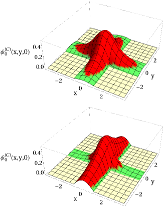
Figure 2: The highly symmetric groundstate $\psi_{0}^{\left(\mathcal{C}\right)}\left(\mathbf{r}\right)$ localised around the crossing zone of a wave-guide $\mathcal{C}$ for different choice of tube widths. Upper plot $w_{x}^{\left(\mathcal{C}\right)}=w_{y}^{\left(\mathcal{C}\right)}=w_{z}^{\left(\mathcal{C}\right)}=2L$ , lower plot $w_{x}^{\left(\mathcal{C}\right)}=w_{z}^{\left(\mathcal{C}\right)}=2L$ and $w_{y}^{\left(\mathcal{C}\right)}=0.6w_{x}^{\left(\mathcal{C}\right)}$. Both plots restrict to the plane $z=0$. Length measured in units of $L$.

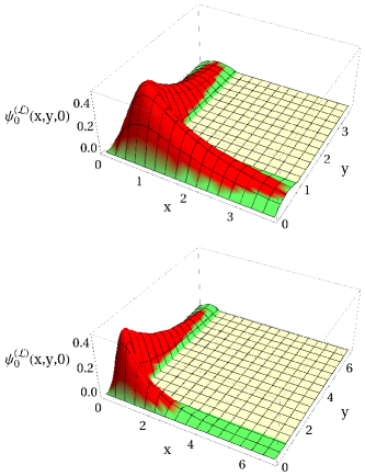
Figure 3: The localised groundstate $\psi_{0}^{\left(\mathcal{L}\right)}\left(\mathbf{r}\right)$ around the corner zone of an $L$-shaped waveguide $\mathcal{L}$ for different choice of tube widths. Upper plot $w_{x}^{\left(\mathcal{L}\right)}=w_{y}^{\left(\mathcal{L}\right)}=L$ and $w_{z}^{\left(\mathcal{L}\right)}=2L$, lower plot $w_{x}^{\left(\mathcal{L}\right)}=L$, $w_{z}^{\left(\mathcal{L}\right)}=2L$ and $w_{y}^{\left(\mathcal{L}\right)}=0.95w_{x}^{\left(\mathcal{L}\right)}$. Both plots restrict to the plane $z=0$. Length measured in units of $L$.

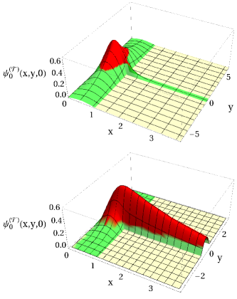
Figure 4: The localised groundstate $\psi_{0}^{\left(\mathcal{T}\right)}\left(\mathbf{r}\right)$ around the branching zone of the $T$-shaped waveguide $\mathcal{T}$ for different choice of tube widths. Upper plot $w_{x}^{\left(\mathcal{T}\right)}=L$, $w_{y}^{\left(\mathcal{T}\right)}=0.6L$ and $w_{z}^{\left(\mathcal{T}\right)}=2L$ , lower plot $w_{y}^{\left(\mathcal{T}\right)}=1.2L$, $w_{x}^{\left(\mathcal{T}\right)}=L$ and $w_{z}^{\left(\mathcal{T}\right)}=2L$. Both plots restrict to the plane $z=0$. Length measured in units of $L$.

In Fig.5 we display for all three waveguides $\Gamma\in\left\{\mathcal{C},\mathcal{T},\mathcal{L}\right\}$ the eigenvalues $E_{0\ }^{\left(\Gamma\right)}$ of the associated ground state eigenmode $\psi_{0\ }^{\left(\Gamma\right)}(\mathbf{r})$ , plotting the ratios $E_{0\ }^{\left(\Gamma\right)}/\varepsilon_{xt\ }^{\left(\Gamma\right)}$ as a function of the thickness parameter $w_{z}^{\left(\Gamma\right)}$ of the respective waveguides, restricting to a symmetric choice of tube widths, $\kappa^{\left(\Gamma\right)}\equiv w_{y}^{\left(\Gamma\right)}/w_{x}^{\left(\Gamma\right)}=1$. In the limit of a thin layer, $w_{z}^{\left(\Gamma\right)}\rightarrow 0$ , there holds $E_{0\ }^{\left(\Gamma\right)}\rightarrow\varepsilon_{xt\ }^{\left(\Gamma\right)}$. For thick layers (not a ’thin’ film) corresponding to the planar limit $w_{z}^{\left(\Gamma\right)}\rightarrow\infty$ (two-dimensional Laplace operator), calculations based on our heat kernel method confirm the eigenvalue $E_{0\ }^{\left(\mathcal{C}\right)}=0.659$ $\times\varepsilon_{xt\ }^{\left(\mathcal{C}\right)}$ for the ground state $\psi_{0\ }^{\left(\mathcal{C}\right)}(\mathbf{r})$ for a symmetric crossing $\mathcal{C}$ with $\kappa^{\left(\mathcal{C}\right)}=1$ , and the eigenvalue $E_{0\ }^{\left(\mathcal{L}\right)}=0.929$ $\times\varepsilon_{xt\ }^{\left(\mathcal{L}\right)}$for the ground state $\psi_{0\ }^{\left(\mathcal{L}\right)}(\mathbf{r})$ for a symmetric cranked waveguide $\mathcal{L}$ with $\kappa^{\left(\mathcal{L}\right)}=1$, in complete agreement with previous calculations srw , ez2 , Amore , Avishai , Trefethen I based on solving the two-dimensional Schrödinger eigenvalue problem with a variational collocation ansatz.

We find that the eigenvalue $E_{0\ }^{\left(\Gamma\right)}$ of the ground state modes $\psi_{0\ }^{\left(\Gamma\right)}(\mathbf{r})$ of a massive particle moving inside a realistic thin film or three-dimensional QW depends indeed strongly on the thickness parameter $w_{z}^{\left(\Gamma\right)}$, as can be seen from the results displayed in Fig.5, Fig.6. While the eigenvalues $E_{0\ }^{\left(\Gamma\right)}$certainly depend on $w_{z}^{\left(\Gamma\right)}$, the localisation lengths $\lambda_{x}^{\left(\Gamma\right)}$ and $\lambda_{y}^{\left(\Gamma\right)}$ of the eigenmodes $\psi_{0\ }^{\left(\Gamma\right)}(\mathbf{r})$ along the respective tube axes $\mathbf{e}_{x}$ and $\mathbf{e}_{y}$ of the waveguides $\Gamma\in\left\{\mathcal{C},\mathcal{T},\mathcal{L}\right\}$ are independent on the tickness parameter $w_{z}^{\left(\Gamma\right)}$, because at a large distance to the respective branching zones of $\Gamma$ the Schrödinger eigenvalue problem (6) is completely separable.

For an asymmetric crossing of two waveguides with different tube widths, assuming $w_{y}^{\left(\mathcal{C}\right)}<w_{x}^{\left(\mathcal{C}\right)}$, see Fig.1, the localised ground state $\psi_{0\ }^{\left(\mathcal{C}\right)}(\mathbf{r})$ then decays exponentially along the axes $\mathbf{e}_{x}$ and $\mathbf{e}_{y}$ of $\mathcal{C}$, displaying a smaller decay length $\lambda_{x}^{\left(\mathcal{C}\right)}$ along the tube axes $\pm\mathbf{e}_{x}$ of the arms with shorter lateral size $w_{y}^{\left(\mathcal{C}\right)}$, and a larger decay length $\lambda_{y}^{\left(\mathcal{C}\right)}$ along the tube axes $\pm\mathbf{e}_{y}$ of the arms with wider lateral size $w_{x}^{\left(\mathcal{C}\right)}$.

While there always exists a localised ground state $\psi_{0\ }^{\left(\mathcal{C}\right)}(\mathbf{r})$ around the crossing zone $\mathcal{A}_{0}\subset$ $\mathcal{C}$ for any choice of tube widths $w_{y}^{\left(\mathcal{C}\right)}\$and $w_{x}^{\left(\mathcal{C}\right)}$, see Fig.7, a localised ground state $\psi_{0\ }^{\left(\mathcal{L}\right)}(\mathbf{r})$ around the corner of the cranked $L$-shaped waveguide $\mathcal{L}$ only exists if the tube widths ratio $\kappa^{\left(\mathcal{L}\right)}=\frac{w_{y}^{\left(\mathcal{L}\right)}}{w_{x}^{\left(\mathcal{L}\right)}}$ is not too small, i.e. a localised ground state exists provided $\kappa_{c}^{\left(\mathcal{L}\right)}<\kappa^{\left(\mathcal{L}\right)}\$, with $\kappa_{c}^{\left(\mathcal{L}\right)}$ denoting a characteristic lower bound of tube widths ratios. Choosing $w_{z}^{\left(\mathcal{L}\right)}=2L=w_{x}^{\left(\mathcal{L}\right)}$ we obtain from our three-dimensional numerical calculations a value around $\kappa_{c}^{\left(\mathcal{L}\right)}\simeq\allowbreak 0.89$ , see Fig.7.

On the other hand, for an asymmetric wave guide $\mathcal{T}$ a localised ground state $\psi_{0\ }^{\left(\mathcal{T}\right)}(\mathbf{r})$ around the branching zone of $\mathcal{T}$ only exists, if the ratio $\kappa^{\left(\mathcal{T}\right)}=\frac{w_{y}^{\left(\mathcal{T}\right)}}{w_{x}^{\left(\mathcal{T}\right)}}$ is not too big, i.e. a localised ground state exists provided $0<\kappa^{\left(\mathcal{T}\right)}<\kappa_{c}^{\left(\mathcal{T}\right)}$. Choosing $w_{z}^{\left(\mathcal{T}\right)}=L=w_{x}^{\left(\mathcal{T}\right)}$ we find from our three-dimensional numerical calculations a value around $\kappa_{c}^{\left(\mathcal{T}\right)}\simeq 1.26$ , see Fig.7.

Similar (equivalent) results for asymmetric (but planar) waveguides were recently obtained by Nazarov Nazarov II , and independently by Amore et al. Amore using precise numerical collocation (using many grid points). Coupled waveguide geometries of finite extension may also display a high sensitivity of the localisation of the ground state mode to slight changes of the geometrical shape dng , dng1 .

A possible physical explanation why for a single particle a localised ground state ceases to exist around the corner zone in $\mathcal{L}$ for $\kappa^{\left(\mathcal{L}\right)}\leq\kappa_{c}^{\left(\mathcal{L}\right)}$, and likewise ceases to exist around the branching zone in $\mathcal{T}$ for $\kappa_{c}^{\left(\mathcal{T}\right)}\leq\kappa^{\left(\mathcal{T}\right)}$, but always exists around the crossing zone $\mathcal{A}_{0}\subset\mathcal{C}$ for any $\kappa^{\left(\mathcal{C}\right)}>0$, we discuss in the next section III

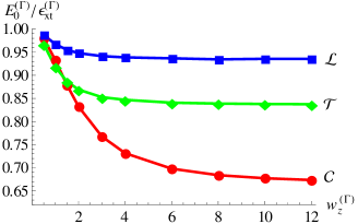
Figure 5: The ratio $E_{0}^{\left(\Gamma\right)}/\varepsilon_{xt}^{\left(\Gamma\right)}$ of the eigenvalue $E_{0}^{\left(\Gamma\right)}$ to the threshold energy $\varepsilon_{xt\ }^{\left(\Gamma\right)}$ corresponding to the localised groundstate mode $\psi_{0}^{\left(\Gamma\right)}\left(\mathbf{r}\right)$ in the respective waveguide geometries $\Gamma\in\left\{\mathcal{C},\mathcal{T},\mathcal{L}\right\}$ as a function of the tube height $w_{z}^{\left(\Gamma\right)}$, assuming fixed tube widths $w_{x}^{\left(\Gamma\right)}=w_{y}^{\left(\Gamma\right)}$. Length measured in units of $L$.

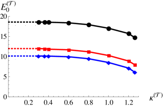
Figure 6: The eigenvalue $E_{0}^{\left(\mathcal{T}\right)}$ of the localised groundstate mode $\psi_{0}^{\left(\mathcal{T}\right)}\left(\mathbf{r}\right)$ in the $T$-shaped waveguide geometry vs. the lateral tube widths ratio $\kappa^{\left(\mathcal{T}\right)}=w_{y}^{\left(\mathcal{T}\right)}/w_{x}^{\left(\mathcal{T}\right)}$ assuming different tube heights: $w_{z}^{\left(\mathcal{T}\right)}=L$ (black), $w_{z}^{\left(\mathcal{T}\right)}=2L$ (red), $w_{z}^{\left(\mathcal{T}\right)}=4L$ (blue). Energy measured in units of $\varepsilon_{L}$.

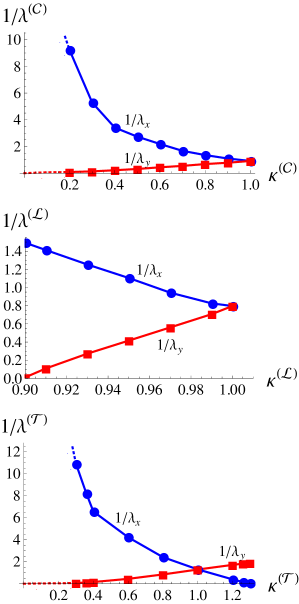
Figure 7: Inverse localisation lengths $1/\lambda_{y}^{\left(\Gamma\right)}$ along tube axis $\mathbf{e}_{y}$ (red line) and $1/\lambda_{x}^{\left(\Gamma\right)}$ along tube axis $\mathbf{e}_{x}$ (blue line) of prototype waveguides $\Gamma\in\left\{\mathcal{C},\mathcal{L},\mathcal{T}\right\}$ as function of respective tube widths ratio $\kappa^{\left(\Gamma\right)}=w_{y}^{\left(\Gamma\right)}/w_{x}^{\left(\Gamma\right)}$ for constant tube height $w_{z}^{\left(\Gamma\right)}=2L$. Upper plot $w_{x}^{\left(\mathcal{C}\right)}=2L$, middle plot $w_{x}^{\left(\mathcal{L}\right)}=L$, lower plot $w_{x}^{\left(\mathcal{T}\right)}=L$. If $\kappa^{\left(\mathcal{L}\right)}<\kappa_{c}^{\left(\mathcal{L}\right)}\simeq 0.89$ no localised ground state $\psi_{0}^{\left(\mathcal{L}\right)}\left(\mathbf{r}\right)$ exists, if $\kappa^{\left(\mathcal{T}\right)}>\kappa_{c}^{\left(\mathcal{T}\right)}\simeq 1.26$ no localised ground state $\psi_{0}^{\left(\mathcal{T}\right)}\left(\mathbf{r}\right)$ exists. Length measured in units of $L$.

III Reason for Non Standard Trapping Around Branching Zones in Quantum Waveguides

Besides bouncing back and forth from the hard walls a classical particle senses no extra force when it moves, say along the tube axis $\mathbf{e}_{y}$, inside the cross shaped waveguide $\mathcal{C}$. The question is then, why in quantum mechanics the ground state $\psi_{0}^{\left(\mathcal{C}\right)}(\mathbf{r})$ of a particle moving inside $\mathcal{C}$ is always localised around the crossing zone $\mathcal{A}_{0}\subset\mathcal{C}$ with an eigenvalue $E_{0}^{\left(\mathcal{C}\right)}$ below the excitation threshold $\varepsilon_{xt}^{\left(\mathcal{C}\right)}$. The key observation to answer this question is, that far from the crossing zone $\mathcal{A}_{0}$, say deep inside the arms $\mathcal{A}_{2}$ and $\mathcal{A}_{4}$, the Schrödinger eigenvalue problem is separable, so that $\psi_{0}^{\left(\mathcal{C}\right)}\left(\mathbf{r}\right)=\psi_{\perp}^{\left(\mathcal{C}\right)}\left(\mathbf{r}_{\perp}\right)\phi_{0}^{\left(\mathcal{C}\right)}(y)$. Introducing the function

$$\phi_{0}^{\left(\mathcal{C}\right)}(y)=\int_{-\infty}^{\infty}dx\int_{-L_{z}}^{L_{z}}dz\ \psi_{\perp}^{\left(\mathcal{C}\right)}\left(\mathbf{r}\right)\psi_{0}^{\left(\mathcal{C}\right)}\left(\mathbf{r}\right)$$ (21)

we see that (6) is equivalent to a one-dimensional Schrödinger eigenvalue problem

$$\left[-\partial_{y}^{2}+V_{\perp}^{\left(\mathcal{C}\right)}(y)\right]\phi_{0}^{\left(\mathcal{C}\right)}(y)=E_{0}^{\left(\mathcal{C}\right)}\phi_{0}^{\left(\mathcal{C}\right)}(y)$$ (22)

, but with an effective potential $V_{\perp}^{\left(\mathcal{C}\right)}(y)$ generated by the transversal kinetic energy,

$$V_{\perp}^{\left(\mathcal{C}\right)}(y)=\frac{\int_{-\infty}^{\infty}dx\int_{-L_{z}}^{L_{z}}dz\ \psi_{\perp}^{\left(\mathcal{C}\right)}\left(\mathbf{r}\right)\left(-\partial_{x}^{2}-\partial_{z}^{2}\right)\psi_{0}^{\left(\mathcal{C}\right)}\left(\mathbf{r}\right)}{\int_{-\infty}^{\infty}dx\int_{-L_{z}}^{L_{z}}dz\ \psi_{0}^{\left(\mathcal{C}\right)}\left(\mathbf{r}\right)\psi_{\perp}^{\left(\mathcal{C}\right)}\left(\mathbf{r}\right)}$$ (23)

, as the coordinate $y$ runs along the tube axis $\mathbf{e}_{y}$.

III.1 Non Standard Trapping in $\mathcal{C}$.

For example, consider equal tube diameters $w_{x}^{\left(\mathcal{C}\right)}=w_{y}^{\left(\mathcal{C}\right)}=w_{z}^{\left(\mathcal{C}\right)}=2L$. Then a rather accurate fit to the spatial variation of the transversal part $\psi_{\perp}^{\left(\mathcal{C}\right)}\left(\mathbf{r}\right)$ of the numerically calculated three-dimensional ground state wave function $\psi_{0}^{\left(\mathcal{C}\right)}\left(\mathbf{r}\right)$ inside the respective tube segments $\mathcal{A}_{j}$ is

$$\psi_{\perp}^{\left(\mathcal{C}\right)}\left(\mathbf{r}\right)=\left\{\begin{array}[]{c}a_{\perp}\cos\left(\frac{\pi}{2L}x\right)\cos\left(\frac{\pi}{2L_{z}}z\right)\text{ for }\mathbf{r\in}\mathcal{A}_{2}\cup\mathcal{A}_{4}\\ \frac{a_{\perp}}{\cosh^{2}\left(\frac{x}{2\lambda}\right)}\cos\left(\frac{\pi}{2L_{z}}z\right)\text{for }\mathbf{r\in}\mathcal{A}_{0}\cup\mathcal{A}_{1}\cup\mathcal{A}_{3}\\ 0\text{ for }\mathbf{r\notin}\mathcal{C}\end{array}\right.$$

Here, the length $\lambda$ is equal to the numerically determined localisation length of the three-dimensional ground state wave function $\psi_{0}^{\left(\mathcal{C}\right)}\left(\mathbf{r}\right)$ for a single particle, see Fig.2.

As can be seen in Fig.8, the effective potential $V_{\perp}^{\left(\mathcal{C}\right)}(y)$ calculated from (23) takes on the form of a one-dimensional box-shaped potential as one traverses the crossing zone $\mathcal{A}_{0}\subset\mathcal{C}$ along the tube axis $\mathbf{e}_{y}$:

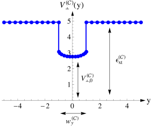
Figure 8: Effective one-dimensional potential $V_{\perp}^{\left(\mathcal{C}\right)}(y)\$ vs. $y$ as sensed by a particle traversing the crossing region of the waveguide $\mathcal{C}$. Length and energy measured in units of $L$ and $\varepsilon_{L}$, respectively.

$$V_{\perp}^{\left(\mathcal{C}\right)}(y)=\left\{\begin{array}[]{c}V_{\perp,0}^{\left(\mathcal{C}\right)}\text{\ for }\left|y\right|<L\\ \varepsilon_{xt}^{\left(\mathcal{C}\right)}\text{ for }\left|y\right|>L\end{array}\right.$$ (24)

, with $\varepsilon_{xt}^{\left(\mathcal{C}\right)}=\lim_{\left|y\right|\rightarrow\infty}V_{\perp}^{\left(\mathcal{C}\right)}(y)>V_{\perp,0}^{\left(\mathcal{C}\right)}\geq 0$ denoting here the excitation threshold in the arms $\mathcal{A}_{2}$ , $\mathcal{A}_{4}$. Actually there holds $\varepsilon_{xt}^{\left(\mathcal{C}\right)}>V_{\perp,0}^{\left(\mathcal{C}\right)}$ for arbitrary cross shaped waveguides $\mathcal{C}$, so the potential $V_{B}^{\left(\mathcal{C}\right)}(y)$ is always attractive and has therefore a finite binding strength (scaled units)

$$b_{\perp\ }^{\left(\mathcal{C}\right)}=\sqrt{\varepsilon_{xt}^{\left(\mathcal{C}\right)}-V_{\perp,0}^{\left(\mathcal{C}\right)}}$$ (25)

The existence of a bound state with even parity localised inside the box $\left|y\right|<L$ is then granted (see any standard text on Quantum Mechanics, e.g. QM ). So it is the rapid change of the transversal kinetic energy that occurs in our waveguide system around the crossing zone $\mathcal{A}_{0}\subset\mathcal{C}$ , see Figure (1), that provides the physical mechanism for trapping a quantum particle of mass $m$ in that region. Via the excitation threshold $\varepsilon_{xt}^{\left(\mathcal{C}\right)}$ , see 10, the strength of this unconventional trapping force is not only dependent on the respective tube sizes $w_{a}^{\left(\mathcal{C}\right)}$ , but also dependent on mass, a lighter particle thus experiencing a stronger trapping force than a heavier one!

Because for an attractive one-dimensional box-shaped potential $V_{\perp}^{\left(\mathcal{C}\right)}(y)$ there always exists a localised ground state with even parity for any value of the binding strength $b_{\perp\ }^{\left(\mathcal{C}\right)}>0$, one may further simplify the problem. Being only interested in the asymptotic behaviour of the ground state $\phi_{0}^{\left(\mathcal{C}\right)}(y)$ at a large distance $\left|y\right|>>L$ to the crossing zone $\mathcal{A}_{0}$ , we may replace $V_{\perp}^{\left(\mathcal{C}\right)}(y)$ by an equivalent attractive delta function potential (scaled units):

$$V_{\perp}^{\left(\mathcal{C}\right)}(y)\rightarrow\widetilde{V}_{\perp}^{\left(\mathcal{C}\right)}(y)=\varepsilon_{xt}^{\left(\mathcal{C}\right)}-\frac{2}{\lambda}\delta(y)$$ (26)

The associated normalised bound state wave function $\widetilde{\phi}_{0}^{\left(\mathcal{C}\right)}(y)$ is then (see any standard text on Quantum Mechanics, for example QM ):

$$\widetilde{\phi}_{0}^{\left(\mathcal{C}\right)}(y)=\sqrt{\frac{1}{\lambda}}\exp\left(-\frac{\left|y\right|}{\lambda}\right)$$ (27)

This formula provides for $\left|y\right|>>L$ the asymptotic behaviour of the ground state $\phi_{0}^{\left(\mathcal{C}\right)}(y)$. It follows at once that the eigenvalue $E_{0}^{\left(\mathcal{C}\right)}$ associated with $\phi_{0}^{\left(\mathcal{C}\right)}(y)$ is given by (scaled units)

$$E_{0}^{\left(\mathcal{C}\right)}=\varepsilon_{xt}^{\left(\mathcal{C}\right)}-\frac{1}{\lambda^{2}}$$ (28)

In order that such a toy model actually makes sense it is mandatory that $\lambda>L$ , where $w_{y}^{\left(\mathcal{C}\right)}=2L$ measures the lateral size of the crossing zone, see Fig.8. It turns out that our results from the full three-dimensional numerical calculations for the localised ground state $\psi_{0}^{\left(\mathcal{C}\right)}\left(\mathbf{r}\right)$ indeed fulfill this requirement.

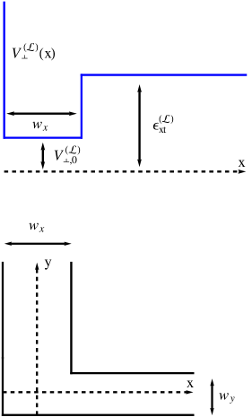
Figure 9: Effective one-dimensional attractive potential $V_{\perp}^{\left(\mathcal{L}\right)}(x)\$ vs. $x$ as sensed by a particle approaching the corner zone of the $L$-shaped waveguide $\mathcal{L}$. Length and energy measured in units of $L$ and $\varepsilon_{L}$, respectively.

III.2 Non Standard Trapping in $\mathcal{L}$.

The cranked $L$-shaped waveguide $\mathcal{L}$ displayed in Fig.1 may be considered as a subdomain (one quarter) of the crossing geometry $\mathcal{C}$. To keep the notation compatible with the one employed to describe the original waveguide $\mathcal{C}$, the height of the tubes comprising $\mathcal{L}$ is denoted as $w_{z}^{\left(\mathcal{L}\right)}=2L_{z}$, while the lateral widths of the tubes with axis $\mathbf{e}_{y}$ and $\mathbf{e}_{x}$, respectively, are denoted as $w_{x}^{\left(\mathcal{L}\right)}=\frac{w_{x}^{\left(\mathcal{C}\right)}}{2}=L$ and $w_{y}^{\left(\mathcal{L}\right)}=\frac{w_{y}^{\left(\mathcal{C}\right)}}{2}=L_{y}$. Traversing the domain $\mathcal{L}$, say parallel to the tube axis $\mathbf{e}_{x}$ , see Fig.1, there results in analogy to the previous consideration for the domain $\mathcal{C}$ an effective one-dimensional Schrödinger eigenvalue problem

$$\left[-\partial_{x}^{2}+V_{\perp}^{\left(\mathcal{L}\right)}(x)\right]\phi_{0}^{\left(\mathcal{L}\right)}(x)=E_{0}^{\left(\mathcal{L}\right)}\phi_{0}^{\left(\mathcal{L}\right)}(x)$$ (29)

Here, the support of $\phi_{0}^{\left(\mathcal{L}\right)}(x)$ is restricted to the half line $x>0$ with the effective one-dimensional potential, see (23), now describing the drop in the transversal kinetic energy around the corner of $\mathcal{L}$ :

$$V_{\perp}^{\left(\mathcal{L}\right)}(x)=\left\{\begin{array}[]{c}\infty\text{ for }x=0\\ V_{\perp,0}^{\left(\mathcal{L}\right)}\text{ for }0<x<L\\ \varepsilon_{xt}^{\left(\mathcal{L}\right)}\ \text{for }L<x\end{array}\right.$$ (30)

The constant $V_{\perp,0}^{\left(\mathcal{L}\right)}$ $<\varepsilon_{xt}^{\left(\mathcal{L}\right)}$ describes the effect, that the transversal kinetic energy may assume a finite value inside the central region $\mathcal{A}_{0}$, possibly also depending on the tube size parameters $w_{a}^{\left(\mathcal{L}\right)}$.

The problem to find the ground state for this potential $V_{\perp}^{\left(\mathcal{L}\right)}(x)$ on the half line $0<x<\infty$ is equivalent to looking for the lowest lying eigenstate with odd parity for an attractive one-dimensional box-shaped potential $V_{\perp}^{\left(\mathcal{C}\right)}(x)$ of the type (24) extended along the full real axis $-\infty<x<\infty$. As is well known, the existence of a localised eigenstate with odd parity for an attractive box-shaped potential like $V_{\perp}^{\left(\mathcal{C}\right)}(x)$ requires a sufficiently strong binding strength (scaled units)

$$b_{\perp\ }^{\left(\mathcal{L}\right)}=\sqrt{\varepsilon_{xt}^{\left(\mathcal{L}\right)}-V_{\perp,0}^{\left(\mathcal{L}\right)}}>\frac{\pi}{2}$$ (31)

(see any standard text on Quantum Mechanics, for example QM ). It is clear from what has been said, that there exists no localised ground state around the corner of a quantum waveguide $\mathcal{L}$ if its tube widths ratio $\kappa^{\left(\mathcal{L}\right)}=\frac{w_{y}^{\left(\mathcal{L}\right)}}{w_{x}^{\left(\mathcal{L}\right)}}$ is below a critical value $\kappa_{c}^{\left(\mathcal{L}\right)}$, in agreement with results obtained from the full three-dimensional numerical calculations presented in Fig.7. As the ratio $\kappa^{\left(\mathcal{L}\right)}$ approaches its lower bound $\kappa_{c}^{\left(\mathcal{L}\right)}$, the binding strength $b_{\perp\ }^{\left(\mathcal{L}\right)}$ approaches (from above) the critical value $\frac{\pi}{2}$, and the localisation length $\lambda$ diverges.

III.3 Non Standard Trapping in $\mathcal{T}$.

Traversing the waveguide $\mathcal{T}$ along the tube axis $\mathbf{e}_{y}$, see Fig.1, the effective one-dimensional potential associated with the drop in the transversal kinetic energy around the braching zone may be described by a potential $V_{\perp}^{\left(\mathcal{T}\right)}\left(x=\frac{w_{x}^{\left(\mathcal{T}\right)}}{2},y\right)$ vs. $y$ similar to the one displayed in Fig.8 for the waveguide $\mathcal{C}$. But traversing $\mathcal{T}$ along the tube axis $\mathbf{e}_{x}$ the corresponding effective potential $V_{\perp}^{\left(\mathcal{T}\right)}\left(x,y=\frac{w_{y}^{\left(\mathcal{T}\right)}}{2}\right)$ vs. $x$ is similar to the one displayed in Fig.9 for the domain $\mathcal{L}$. It follows from what has been said before, that a localised ground state around the branching zone of a $T$-shaped waveguide $\mathcal{T}$ exists only if the ratio of tube widths $\kappa^{\left(\mathcal{T}\right)}=\frac{w_{y}^{\left(\mathcal{T}\right)}}{w_{x}^{\left(\mathcal{T}\right)}}$ is not too large, thus ensuring a large enough binding strength $b_{\perp\ }^{\left(\mathcal{T}\right)}>\frac{\pi}{2}$ of the effective potential $V_{\perp}^{\left(\mathcal{T}\right)}\left(x\right)$, in agreement with the results of the full three-dimensional numerical calculations presented in Fig.7.

IV Localised BEC Ground States Around Branching Zones in $\mathcal{C}$ , $\mathcal{L}$ and $\mathcal{T}$.

To find the optimal GP-orbital $\psi^{\left(\mathcal{C}\right)}(\mathbf{r})$ determining the Hartree ground state (1) of an interacting BEC confined around the crossing zone of the waveguide $\mathcal{C}$ we need to solve the Gross-Pitaevskii equation (3). To construct a suitable splitting scheme we consider an auxiliary diffusion process:

$$-\frac{\partial}{\partial\tau}\psi(\mathbf{r},\tau)=\left[H_{kin}+U_{\psi}(\mathbf{r},\tau)\right]\psi(\mathbf{r},\tau)$$ (32)

However, because the amplitude of the auxiliary wave function $\psi(\mathbf{r},\tau)$ decays exponentially with diffusion time $\tau$ as the diffusion process progresses the interaction term neeeds explicit normalization Krotscheck :

$$U_{\psi}(\mathbf{r},\tau)=\left(N-1\right)\frac{4\pi\hbar^{2}a_{s}}{m}\ \frac{\left|\psi(\mathbf{r},\tau)\right|^{2}}{\int_{\mathcal{C}}d^{3}r^{\prime}\ \left|\psi(\mathbf{r}^{\prime},\tau)\right|^{2}}$$ (33)

Apparently, for large diffusion time $\tau$ then $U_{\psi}(\mathbf{r},\tau)$ becomes independent on $\tau$. The seeked localised GP-orbital is thus given by

$$\psi^{\left(\mathcal{C}\right)}(\mathbf{r})=\lim_{\tau\rightarrow\infty}\frac{\psi(\mathbf{r},\tau)}{\sqrt{\int_{\mathcal{C}}d^{3}r^{\prime}\left|\psi(\mathbf{r}^{\prime},\tau)\right|^{2}}}$$ (34)

In sharp contrast to the behaviour in a harmonic trap, now the kinetic energy in the localised Hartree ground of a BEC, that is confined around the crossing zone $\mathcal{A}_{0}$ of $\mathcal{C}$ by the described non standard trapping force, dominates over the interaction energy even for a large particle number $N$. To solve for a large particle number $N$ the Gross-Pitaevskii equation (3) accurately, a specially tailored splitting scheme is useful as described in the appendix A. The update rule that determines $\psi(\mathbf{r},\tau_{n+1})$ from a given $\psi(\mathbf{r},\tau_{n})$ for a short diffusion time interval $\Delta\tau$ consists of the following five steps:

$$\psi(\mathbf{r},\tau_{0}) = \psi^{\left(in\right)}(\mathbf{r})$$ (35)

$$\tau_{n+1} = \tau_{n}+\Delta\tau\text{ for }n=0,1,2,...$$

$$\psi^{\left(IV\right)}(\mathbf{r},\tau_{n}) = e^{-\frac{\Delta\tau}{6}U_{\psi}(\mathbf{r},\tau_{n})}\psi(\mathbf{r},\tau_{n})$$

$$\psi^{\left(III\right)}(\mathbf{r},\tau_{n}) = \int_{\mathcal{C}}d^{3}\mathbf{r}^{\prime}K(\mathbf{r},\mathbf{r}^{\prime},\frac{\Delta\tau}{2})\psi^{\left(IV\right)}(\mathbf{r}^{\prime},\tau_{n})$$

$$\psi^{\left(II\right)}(\mathbf{r},\tau_{n}) = e^{-\frac{2\Delta\tau}{3}U_{\psi}(\mathbf{r},\tau_{n})}\psi^{\left(III\right)}(\mathbf{r},\tau_{n})$$

$$\psi^{\left(I\right)}(\mathbf{r},\tau_{n}) = \int_{\mathcal{C}}d^{3}\mathbf{r}^{\prime}K(\mathbf{r},\mathbf{r}^{\prime},\frac{\Delta\tau}{2})\psi^{\left(II\right)}(\mathbf{r}^{\prime},\tau_{n})$$

$$\psi(\mathbf{r},\tau_{n+1}) = e^{-\frac{\Delta\tau}{6}U_{\psi}(\mathbf{r},\tau_{n})}\psi^{\left(I\right)}(\mathbf{r},\tau_{n})$$

Here the kernel $K(\mathbf{r},\mathbf{r}^{\prime},\frac{\Delta\tau}{2})$ is associated with the kinetic energy operator $H_{kin}$ of a single particle moving inside $\mathcal{C}$ and obeying to Dirichlet boundary value conditions at the walls $\partial\mathcal{C}$ of that waveguide, see appendix B. It acts on the functions $\psi^{\left(IV\right)}(\mathbf{r}^{\prime},\tau_{n})$ and $\psi^{\left(II\right)}(\mathbf{r}^{\prime},\tau_{n})$ as described in the previous section II.

In the numerical calculations with the proposed splitting scheme we chose $\Delta\tau=0.01\times\left[\frac{\hbar}{\varepsilon_{L}}\right]$. The obtained results clearly show, that the optimal GP-orbital is indeed localised around the crossing zone $\mathcal{A}_{0}$, provided $1\leq N\leq N_{c}^{\left(\mathcal{C}\right)}$, where $N_{c}^{\left(\mathcal{C}\right)}$ denotes a critical particle number depending on the tube sizes $w_{a}^{\left(\mathcal{C}\right)}=2L_{a}$ and the $s$-wave scattering length $a_{s}$ of the Bose atoms. Physically, $N_{c}^{\left(\mathcal{C}\right)}$ has the meaning of the maximal number of particles that can be trapped in the localised Hartree ground state by the described non standard confinement mechanism. In particular, like in the case $N=1$, there exist localised GP-orbitals $\psi_{\gamma}\left(\mathbf{r}\right)$ displaying different discrete symmetries $\gamma\in\left\{A_{g},B_{1g},B_{2u},B_{3u}\right\}$.

Not unexpectedly, the Hartree ground state (1) with the lowest energy in the waveguide system $\mathcal{C}$ is buildt from the orbital $\psi^{\left(\mathcal{C}\right)}(\mathbf{r})\equiv\psi_{A_{g}}\left(\mathbf{r}\right)$ , which orbital is nodeless in $\mathcal{C}$. Like in the single particle case, the optimal GP-orbital $\psi^{\left(\mathcal{C}\right)}(\mathbf{r})$ is localised around the origin $\mathbf{r}=$ $\mathbf{0}$ of the crossing zone $\mathcal{A}_{0}\subset\mathcal{C}$, but the exponential decay of $\psi^{\left(\mathcal{C}\right)}(\mathbf{r})$ with increasing distance to the crossing zone is slower for higher particle numbers $N$, see Fig.10.

A similar behaviour is also found for the other localised GP-orbitals $\psi_{\gamma}\left(\mathbf{r}\right)$ with symmetry representation $\gamma\in\left\{B_{1g},B_{3u}\right\}$, corresponding to the localised GP-orbitals $\psi^{\left(\mathcal{L}\right)}(\mathbf{r})$ and $\psi^{\left(\mathcal{T}\right)}(\mathbf{r})$ comprising the localised BEC ground states around the branching zones of the quantum waveguides $\mathcal{L}$ and $\mathcal{T}$ , respectively. In Fig.11, Fig.12, Fig.13 we show for the waveguides $\mathcal{L}$ and $\mathcal{T}$ the profiles of the localised GP-orbitals $\psi^{\left(\mathcal{L}\right)}(\mathbf{r})$ and $\psi^{\left(\mathcal{T}\right)}(\mathbf{r})$ for different particle numbers $N$. For $N\geq N_{c}^{\left(\Gamma\right)}$ , where $N_{c}^{\left(\Gamma\right)}$ denotes a critical particle number associated with the respective waveguide geometries $\Gamma\in\left\{\mathcal{C},\mathcal{L},\mathcal{T}\right\}$, a localised GP-orbital $\psi^{\left(\Gamma\right)}(\mathbf{r})$ ceases to exist.

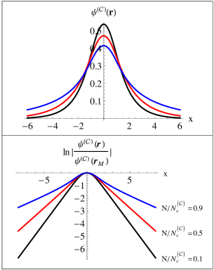
Figure 10: Profile of the GP-orbital $\psi^{(\mathcal{C})}\left(\mathbf{r}\right)$ comprising the Hartree ground state localised around the crossing zone of the waveguide $\mathcal{C}$ for different particle number ratios $N/N_{c}^{\left(\mathcal{C}\right)}$: black line $N/N_{c}^{\left(\mathcal{C}\right)}=0.1$ , red line $N/N_{c}^{\left(\mathcal{C}\right)}=0.5$, blue line $N/N_{c}^{\left(\mathcal{C}\right)}=0.9$. Results shown correspond to tube sizes $w_{x}^{\left(\mathcal{C}\right)}=w_{y}^{\left(\mathcal{C}\right)}=w_{z}^{\left(\mathcal{C}\right)}=2L$. Distance $x$ measured in units of $L$.

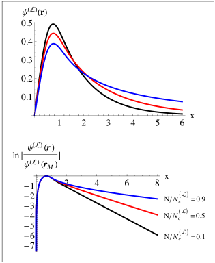
Figure 11: Profile of the GP-orbital $\psi^{(\mathcal{L})}\left(\mathbf{r}\right)$ comprising the Hartree ground state localised around the corner zone of the waveguide $\mathcal{L}$ for different particle number ratios $N/N_{c}^{\left(\mathcal{L}\right)}$: black line $N/N_{c}^{\left(\mathcal{L}\right)}=0.1$ , red line $N/N_{c}^{\left(\mathcal{L}\right)}=0.5$, blue line $N/N_{c}^{\left(\mathcal{L}\right)}=0.9$. Results shown correspond to tube sizes $w_{x}^{\left(\mathcal{L}\right)}=w_{y}^{\left(\mathcal{L}\right)}=L$, $w_{z}^{\left(\mathcal{L}\right)}=2L$. Distance $x$ measured in units of $L$.

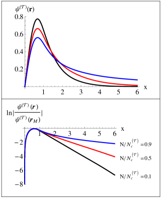
Figure 12: Profile along tube axis direction $\mathbf{e}_{x}$ of the GP-orbital $\psi^{(\mathcal{T})}\left(\mathbf{r}\right)$ comprising the Hartree ground state localised around the branching zone of the waveguide $\mathcal{T}$ for different particle number ratios $N/N_{c}^{\left(\mathcal{T}\right)}$: black line $N/N_{c}^{\left(\mathcal{T}\right)}=0.1$ , red line $N/N_{c}^{\left(\mathcal{T}\right)}=0.5$, blue line $N/N_{c}^{\left(\mathcal{T}\right)}=0.9$. Results shown correspond to tube sizes $w_{x}^{\left(\mathcal{T}\right)}=w_{y}^{\left(\mathcal{T}\right)}=L$, $w_{z}^{\left(\mathcal{T}\right)}=2L$. Distance $x$ measured in units of $L$.

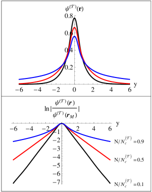
Figure 13: Profile along tube axis direction $\mathbf{e}_{y}$ of the GP-orbital $\psi^{(\mathcal{T})}\left(\mathbf{r}\right)$ comprising the Hartree ground state localised around the branching zone of the waveguide $\mathcal{T}$ for different particle number ratios $N/N_{c}^{\left(\mathcal{T}\right)}$: black line $N/N_{c}^{\left(\mathcal{T}\right)}=0.1$ , red line $N/N_{c}^{\left(\mathcal{T}\right)}=0.5$, blue line $N/N_{c}^{\left(\mathcal{T}\right)}=0.9$. Results shown correspond to tube sizes $w_{x}^{\left(\mathcal{T}\right)}=w_{y}^{\left(\mathcal{T}\right)}=L$, $w_{z}^{\left(\mathcal{T}\right)}=2L$. Distance $y$ measured in units of $L$.

For the determination of the optimal orbital $\psi^{\left(\Gamma\right)}\left(\mathbf{r}\right)$ and the associated chemical potential $\mu_{N}^{\left(\Gamma\right)}$ of the Hartree ground state of the BEC only the effective interaction parameter $\left(N-1\right)$ $\frac{8\pi a_{s}}{L}\$matters (scaled units). As displayed in Fig.14, the critical particle number $N_{c}^{\left(\Gamma\right)}$ displays the expected linear increase as the respective tube diameter $w_{z}^{\left(\Gamma\right)}$ increases.

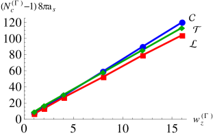
Figure 14: Plot of the critical particle number $N_{c}^{(\Gamma)}-1$ vs. box height $w_{z}^{\left(\Gamma\right)}$ for the cross shaped geometry $\mathcal{C}$ (blue line), $T$-shaped geometry $\mathcal{T}$ (green line) and $L$-shaped geometry $\mathcal{L}$ (red line). Choice of tube width parameters: $w_{x}^{\left(\mathcal{C}\right)}=w_{y}^{\left(\mathcal{C}\right)}=2L$ , $w_{x}^{\left(\mathcal{T}\right)}=w_{y}^{\left(\mathcal{T}\right)}=L$ and $w_{x}^{\left(\mathcal{L}\right)}=w_{y}^{\left(\mathcal{L}\right)}=L$. Tube height $w_{z}^{\left(\Gamma\right)}$ measured in units of $L$.

Once the (normalized!) optimal GP-orbital $\psi^{\left(\Gamma\right)}(\mathbf{r})$ has been found for the respective waveguide geometries $\Gamma\in\left\{\mathcal{C},\mathcal{L},\mathcal{T}\right\}$, it follows directly from (3) by taking a scalar product with the adjoint orbital $\left[\psi^{\left(\Gamma\right)}(\mathbf{r})\right]^{{\dagger}}$ an explicit expression for the Lagrange parameter $\mu_{N}^{\left(\Gamma\right)}$:

$$\mu_{N}^{\left(\Gamma\right)}=\frac{E_{kin}^{\left(\Gamma\right)}\left(N\right)+2E_{int}^{\left(\Gamma\right)}\left(N\right)}{N}$$ (36)

Here

$$E_{int}^{\left(\Gamma\right)}\left(N\right)=\frac{N\left(N-1\right)}{2}\frac{4\pi\hbar^{2}a_{s}}{m}\int_{\Gamma}d^{3}r|\psi^{\left(\Gamma\right)}(\mathbf{r})|^{4}$$ (37)

and

$$E_{kin}^{\left(\Gamma\right)}\left(N\right)=N\int_{\Gamma}d^{3}r\left[\psi^{\left(\Gamma\right)}(\mathbf{r})\right]^{{\dagger}}H_{kin}\psi^{\left(\Gamma\right)}(\mathbf{r})$$ (38)

, respectively, denote the interaction energy and the kinetic energy of the $N$-particle Hartree ground state (1) associated with $\psi^{\left(\Gamma\right)}(\mathbf{r})$. With

$$E^{\left(\Gamma\right)}(N)=E_{kin}^{\left(\Gamma\right)}\left(N\right)+E_{int}^{\left(\Gamma\right)}\left(N\right)$$ (39)

denoting the total energy of the respective $N$-particle Hartree ground states (1) there holds as an identity

$$\mu_{N}^{\left(\Gamma\right)}=E^{\left(\Gamma\right)}(N)-E^{\left(\Gamma\right)}(N-1)$$ (40)

So it is manifest that the Lagrange parameter $\mu_{N}^{\left(\Gamma\right)}$ has the physical meaning of the chemical potential in the ground state of a BEC.

In (15) we plot for the Hartree ground state of a BEC localised around the crossing zone inside $\mathcal{C}$ the ratio of the interaction energy $E_{int}^{\left(\mathcal{C}\right)}$ to the kinetic $E_{kin}^{\left(\mathcal{C}\right)}$ energy vs. particle number $N$. The plot clearly indicates, that such a BEC is dominated by its kinetic energy, so that the profile of the particle density cannot be described by the Thomas-Fermi approximation. A similar behaviour we find for the waveguides $\mathcal{L}$ and $\mathcal{T}$. This finding is in sharp contrast to an interacting cold Bose gas confined in a harmonic trap, where the kinetic energy compared to the interaction energy becomes negligible small for large $N$ proportional to $N\ ^{-\frac{4}{5}}$ .

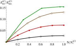
Figure 15: Ratio $E_{int}^{\left(\mathcal{C}\right)}/E_{kin}^{\left(\mathcal{C}\right)}$ as a function of normalized particle number $(N-1)/N_{c}^{\left(\mathcal{C}\right)}$ for the Hartree ground state localised around the crossing zone of the waveguide $\mathcal{C}$. The curves refer to at fixed choice of lateral tube diameters $w_{x}^{\left(\mathcal{C}\right)}=w_{y}^{\left(\mathcal{C}\right)}=2L$, but different tube heights: $w_{z}^{\left(\mathcal{C}\right)}=L$ (open black circles), $w_{z}^{\left(\mathcal{C}\right)}=2L$ (red squares), $w_{z}^{\left(\mathcal{C}\right)}=4L$ (open brown circles), $w_{z}^{\left(\mathcal{C}\right)}=8L$ (green diamonds). Further increase of $w_{z}^{\left(\mathcal{C}\right)}$ gives for $E_{int}^{\left(\mathcal{C}\right)}/E_{kin}^{\left(\mathcal{C}\right)}$ results close to the results obtained for $w_{z}^{\left(\mathcal{C}\right)}=8L$.

The localisation lengths $\lambda_{N,x\ }^{\left(\Gamma\right)}$ and $\lambda_{N,y\ }^{\left(\Gamma\right)}$, which describes the exponential decay of the GP-orbital $\psi^{\left(\Gamma\right)}\left(\mathbf{r}\right)$ away from the localisation zone along the tube axes $\mathbf{e}_{x}$ and $\mathbf{e}_{y}$ of $\Gamma$, are given by

$$1/\lambda_{N,a}^{\left(\Gamma\right)} = -\lim_{s\rightarrow\infty}\frac{1}{\left|\mathbf{r}_{M}+s\mathbf{e}_{a}\right|}\ln\left|\frac{\psi^{\left(\Gamma\right)}\left(\mathbf{r}_{M}+s\mathbf{e}_{a}\right)}{\psi^{\left(\Gamma\right)}\left(\mathbf{r}_{M}\right)}\right|$$ (41)

$$a \in \left\{x,y\right\}$$

, where $\mathbf{r}_{M}$ denotes a suitable reference position, say where the modulus $\left|\psi^{\left(\Gamma\right)}\left(\mathbf{r}\right)\right|$ attains its maximum, see also Fig.10, Fig.11, Fig.12, Fig.13. As a rule the arms of $\Gamma\in\left\{\mathcal{C},\mathcal{L},\mathcal{T}\right\}$ with a narrower lateral diameter are associated with a shorter localisation length.

In Fig.17 the inverse localisation lengths $1/\lambda_{N,x}^{\left(\Gamma\right)}$ and $1/\lambda_{N,y}^{\left(\Gamma\right)}$ are plotted vs. particle number $N$ (using $L$ as unit of length) for two sets of lateral tube diameters with ratio $\kappa^{\left(\Gamma\right)}=\frac{w_{y}^{\left(\Gamma\right)}}{w_{x}^{\left(\Gamma\right)}}$. The green curves refer to a symmetric choice $\kappa^{\left(\Gamma\right)}=1$ assuming $w_{x}^{\left(\mathcal{C}\right)}=2L$, $w_{x}^{\left(\mathcal{L}\right)}=L$, $w_{x}^{\left(\mathcal{T}\right)}=L$ and tube heights $w_{z}^{\left(\Gamma\right)}=2L$. The blue and red curves refer to an asymmetric choice of tube widths, $\kappa^{\left(\mathcal{C}\right)}=0.8$ , $\kappa^{\left(\mathcal{L}\right)}=0.95$, $\kappa^{\left(\mathcal{T}\right)}=0.8$. The results of our full three-dimensional numerical calculations clearly show that depending on the choice of $\kappa^{\left(\Gamma\right)}$ the localisation length along the arms of wider lateral diameter commences to diverge when the particle number $N$ approaches the critical particle number $N_{c}^{\left(\Gamma\right)}=N_{c}^{\left(\Gamma\right)}\left(w_{x}^{\left(\Gamma\right)},w_{y}^{\left(\Gamma\right)},w_{z}^{\left(\Gamma\right)}\right)$. Apparently the inverse of the larger localisation length scales linearly with particle number $N$ over the full range $1\leq N\leq N_{c}^{\left(\Gamma\right)}$.

For the chemical potential $\mu_{N}^{\left(\Gamma\right)}$ of the localised Hartree ground state inside the respective waveguides $\Gamma\in\left\{\mathcal{C},\mathcal{T},\mathcal{L}\right\}$ there holds $0<\mu_{N}^{\left(\Gamma\right)}<\varepsilon_{xt}^{\left(\Gamma\right)}$. In Fig.18 we plot the square root $\sqrt{\varepsilon_{xt}^{\left(\Gamma\right)}-\mu_{N}^{\left(\Gamma\right)}}$ of the difference of the excitation threshold $\varepsilon_{xt}^{\left(\Gamma\right)}$ to the chemical potential $\mu_{N}^{\left(\Gamma\right)}$ vs. particle number $N$ choosing the respective tube diameters like in Fig.17. A linear decrease with increasing particle number $N$ of the function $\sqrt{\varepsilon_{xt}^{\left(\Gamma\right)}-\mu_{N}^{\left(\Gamma\right)}}$ is clearly visible in all results of our numerical calculations over the full range $1\leq N\leq N_{c}^{\left(\Gamma\right)}$. For $N\ \rightarrow N_{c}^{\left(\Gamma\right)}$ with $N_{c}^{\left(\Gamma\right)}=N_{c}^{\left(\Gamma\right)}\left(w_{x}^{\left(\Gamma\right)},w_{y}^{\left(\Gamma\right)},w_{z}^{\left(\Gamma\right)}\right)$ the chemical potential $\mu_{N}^{\left(\Gamma\right)}$ approaches the excitation threshold $\varepsilon_{xt}^{\left(\Gamma\right)}$ for a single particle. We find excellent agreement of the numerical results for $\mu_{N}^{\left(\Gamma\right)}$ with the following scaling relation

$$\frac{\mu_{N=N_{c}}^{\left(\Gamma\right)}-\mu_{N}^{\left(\Gamma\right)}}{\mu_{N=N_{c}}^{\left(\Gamma\right)}-\mu_{N=1}^{\left(\Gamma\right)}}=\left(1-\frac{N-1}{N_{c}^{\left(\Gamma\right)}-1}\right)^{2}$$ (42)

The displayed apparent linear scaling of $\sqrt{\mu_{N=N_{c}}^{\left(\Gamma\right)}-\mu_{N}^{\left(\Gamma\right)}}$ vs. particle number $N$ is in sharp contrast to the well known scaling $\mu_{N}$ $\varpropto N^{\frac{2}{5}}$ of the chemical potential $\mu_{N}$ in a conventional harmonic atom trap Pethick&Smith . Though for (anharmonic) shallow atom trap potentials there also exists a critical particle number $N_{c}$, only small deviations to the scaling $\mu_{N}$ $\varpropto N^{\frac{2}{5}}$ have been reported Martikainen . For comparison we show in Fig. 16 the function $\sqrt{\mu_{N=N_{c}}-\mu_{N}}$ as obtained for shallow conservative trap potentials Martikainen , and also for a harmonic trap of finite depth. It is clearly visible, that the described non standard trapping around a crossing or branching zone of a QW with regard to the dependence on particle number $N$ noticeably differs from results obtained for conservative trap potentials.

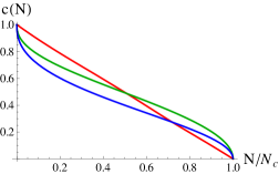
Figure 16: The function $c\left(N\right)=\sqrt{\frac{\mu_{N=N_{c}}-\mu_{N}}{\mu_{N=N_{c}}-\mu_{N=1}}}$ vs. normalized particle numbers $N/N_{c}$ for chemical potential $\mu_{N}$ corresponding to: (i) a shallow conservative trap potential as considered in Ref.Martikainen (blue line), (ii) a harmonic trap potential of finite depth (green line), (iii) the non standard trapping around the crossing of a QW (red line). The particle number $N_{c}$ denotes the maximum number of particles in the respective traps.

In Fig.19 we display the effect interactions have on the localisation length $1/\lambda_{N,x}^{\left(\Gamma\right)}$ and $1/\lambda_{N,y}^{\left(\Gamma\right)}$ of the ground state of a BEC for various particle numbers $N$ as a function of the ratio $\kappa^{\left(\Gamma\right)}=\frac{w_{y}^{\left(\Gamma\right)}}{w_{x}^{\left(\Gamma\right)}}$ of lateral tube diameters (we assume $w_{y}^{\left(\mathcal{C}\right)}\leq w_{x}^{\left(\mathcal{C}\right)}$). The previously established bounds for the localisation of a single particle are clearly changed, see Fig.7. According to our numerical calculations a localised Hartree ground state exists (i) around the crossing zone of the waveguide $\mathcal{C}\$ only for $\kappa_{c}^{\left(\mathcal{C}\right)}\left(N\right)<\ \kappa^{\left(\mathcal{C}\right)}$, (ii) around the corner of the waveguide $\mathcal{L}$ only for $\kappa_{c}^{\left(\mathcal{L}\right)}\left(N\right)<\kappa^{\left(\mathcal{L}\right)}$ , and (iii) around the branching zone of the waveguide $\mathcal{T}$ only in the interval $\kappa_{c,1}^{\left(\mathcal{T}\right)}\left(N\right)<\ \kappa^{\left(\mathcal{T}\right)}<\kappa_{c,2}^{\left(\mathcal{T}\right)}\left(N\right)$. We find all the lower bounds $\kappa_{c}^{\left(\mathcal{C}\right)}\left(N\right)$, $\kappa_{c}^{\left(\mathcal{L}\right)}\left(N\right)$ and $\kappa_{c,1}^{\left(\mathcal{T}\right)}\left(N\right)$ increase as $N$ increases, while the upper bound $\kappa_{c,2}^{\left(\mathcal{T}\right)}\left(N\right)$ decreases as $N$ increases.

The observed scaling laws for the localisation lengths $\lambda_{N,a}^{\left(\Gamma\right)}$ (see Fig. 17) and the non standard scaling law of the chemical potential $\mu_{N}^{\left(\Gamma\right)}$ vs. particle number $N$ (see Fig. 18), as obtained from our full three-dimensional numerical calculations, can be explained in terms of analytical results derived from a simple toy model that we discuss in section V.

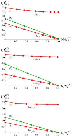
Figure 17: The inverse localisation lengths $1/\lambda_{N,x}^{\left(\Gamma\right)}$ and $1/\lambda_{N,y}^{\left(\Gamma\right)}$ along the respective tube axes $\mathbf{e}_{x}$ and $\mathbf{e}_{y}$ vs. particle number $N$ of the Hartree ground state of a BEC localised around the crossing or branching zone of three prototype waveguides $\Gamma\in\left\{\mathcal{C},\ \mathcal{L},\mathcal{T}\right\}$. All plots refer to a tube height $w_{z}^{\left(\Gamma\right)}=2L$. All green lines (S) correspond to a symmetric choice of lateral tube diameters $w_{y}^{\left(\Gamma\right)}=w_{x}^{\left(\Gamma\right)}$, all red lines (A) correspond to an asymmetric choice $w_{y}^{\left(\Gamma\right)}<w_{x}^{\left(\Gamma\right)}$.  1) waveguide $\mathcal{C}$ : $w_{x}^{\left(\mathcal{C}\right)}=2L$, $w_{y}^{\left(\mathcal{C}\right)}=0.8w_{x}^{\left(\mathcal{C}\right)}$. 2) waveguide $\mathcal{L}$ : $w_{x}^{\left(\mathcal{L}\right)}=L$, $w_{y}^{\left(\mathcal{L}\right)}=0.95w_{x}^{\left(\mathcal{L}\right)}$. 3) waveguide $\mathcal{T}$ : $w_{x}^{\left(\mathcal{T}\right)}=L$, $w_{y}^{\left(\mathcal{T}\right)}=0.8w_{x}^{\left(\mathcal{T}\right)}$. In all plots $L$ denotes the unit of length.

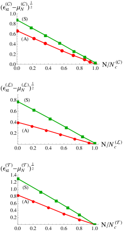
Figure 18: The chemical potential $\mu_{N}^{\left(\Gamma\right)}$ vs. particle number $N$ of the Hartree ground state of a BEC localised around the crossing or branching zone of three prototype waveguides $\Gamma\in\left\{\mathcal{C},\ \mathcal{L},\mathcal{T}\right\}$. All plots refer to a tube height $w_{z}^{\left(\Gamma\right)}=2L$. All green lines (S) correspond to a symmetric choice of lateral tube diameters $w_{y}^{\left(\Gamma\right)}=w_{x}^{\left(\Gamma\right)}$, all red lines (A) correspond to an asymmetric choice $w_{y}^{\left(\Gamma\right)}<w_{x}^{\left(\Gamma\right)}$.  1) waveguide $\mathcal{C}$ : $w_{x}^{\left(\mathcal{C}\right)}=2L$, $w_{y}^{\left(\mathcal{C}\right)}=0.8w_{x}^{\left(\mathcal{C}\right)}$. 2) waveguide $\mathcal{L}$ : $w_{x}^{\left(\mathcal{L}\right)}=L$, $w_{y}^{\left(\mathcal{L}\right)}=0.95w_{x}^{\left(\mathcal{L}\right)}$. 3) waveguide $\mathcal{T}$ : $w_{x}^{\left(\mathcal{T}\right)}=L$, $w_{y}^{\left(\mathcal{T}\right)}=0.8w_{x}^{\left(\mathcal{T}\right)}$. In all plots $\varepsilon_{L}$ denotes the unit of energy.

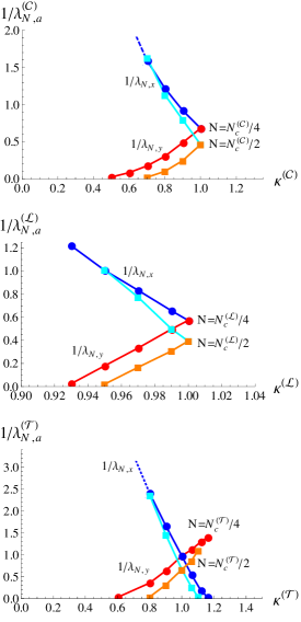
Figure 19: Inverse localisation length $1/\lambda_{N,y}^{\left(\Gamma\right)}$ (red and orange line) and $1/\lambda_{N,x}^{\left(\Gamma\right)}$ (blue and cyan line) of the Hartree ground state in the quantum waveguides $\Gamma\in\left\{\mathcal{C},\mathcal{L},\mathcal{T}\right\}$ for different ratios $\kappa^{\left(\Gamma\right)}=w_{y}^{\left(\Gamma\right)}/w_{x}^{\left(\Gamma\right)}$ of lateral tube diameters. Curves shown refer to two choices of particle numbers: $N=0.25N_{c}^{\left(\Gamma\right)}$ and $N=0.5N_{c}^{\left(\Gamma\right)}$. Here $N_{c}^{\left(\Gamma\right)}$ denotes the critical particle number of the respective waveguide assuming $\kappa^{\left(\Gamma\right)}=1$. Tube height is for all plots $w_{z}^{\left(\Gamma\right)}=2L$, lateral tube widths are $w_{x}^{\left(\mathcal{C}\right)}=2L$, $w_{x}^{\left(\mathcal{L}\right)}=L$, $w_{x}^{\left(\mathcal{T}\right)}=L$.  In all plots $L$ denotes the unit of length.

V Scaling Laws for Localisation Length and Chemical Potential vs. Particle Number $N$ from a Toy Model.

When a single atom traverses the crossing zone $\mathcal{A}_{0}$ of size $2L$ of the waveguide $\mathcal{C}$ its transversal kinetic energy undergoes a sudden drop. As shown already in section III for a single particle, see also lp0 , the influence of this sudden drop on the asymptotic decay of the ground state can be modelled by an attractive delta-function potential $-\frac{2}{\lambda}\delta(x)$ , corresponding to a localisation length $\lambda>L$. Such a delta-function potential is equivalent to a jump condition for the first derivative of the wave function taken at $x=0$:

$$\left[\partial_{x}\phi(x)\ \right]_{x=0^{-}}^{x=0^{+}}\ =-\frac{2}{\lambda}\phi(0)$$ (43)

The Gross Pitaevskii equation (3) determining the $N$-particle Hartree ground state (1) of a BEC in terms of the optimal GP-orbital $\psi^{\left(\mathcal{C}\right)}\left(\mathbf{r}\right)$ can be projected at large distance $x$ to the crossing zone $\mathcal{A}_{0}$ to one dimension making the separation ansatz

$$\psi^{\left(\mathcal{C}\right)}\left(\mathbf{r}\right)\rightarrow\psi_{\perp}^{\left(\mathcal{C}\right)}\left(\mathbf{r}_{\perp}\right)\phi(x)$$

The function $\phi_{N}(x)$ in this case solves a one-dimensional non linear Schrödinger equation (scaled units):

$$\left[-\partial_{x}^{2}+\varepsilon_{xt}-\mu_{N}-\frac{2}{\lambda_{N}}\delta(x)+\left(N-1\right)g_{s}\left|\phi(x)\right|^{2}\right]\phi(x)=0$$ (44)

Here $g_{s}$ describes the strength of the effective repulsive two-body interaction potential (as projected to one-dimension), and $\mu_{N}$ is the chemical potential ensuring the usual normalization constraint of the GP-orbital.

To solve this differential equation we make an ansatz for $\phi(x)$ depending on three parameters, the amplitude $A_{N}$ , the localisation length $\lambda_{N}>0$ and a shift parameter $s_{N}>0$ :

$$\phi_{N}\left(x\right)=\frac{A_{N}}{\sinh\left(\frac{|x|+s_{N}}{\lambda_{N}}\right)}$$ (45)

This ansatz solves (44) and the boundary condition (43), provided

$$\mu_{N} = \varepsilon_{xt}-\frac{1}{\lambda_{N}^{2}}$$ (46)

$$\lambda_{N} = \frac{\lambda}{1-\frac{\left(N-1\right)g_{s}\lambda}{4}}>0$$

$$\exp\left(-\frac{s_{N}}{\lambda_{N}}\right) = \sqrt{\frac{\frac{\lambda_{N}}{\lambda}-1}{\frac{\lambda_{N}}{\lambda}+1}}$$

$$A_{N} = \frac{1}{\sqrt{2\lambda_{N}\left(\frac{\lambda_{N}}{\lambda}-1\right)}}$$

The amplitude $A_{N}$ is fixed by the usual wavefunction normalization. Apparently, for $N\rightarrow 1$ there holds $\lambda_{N}\rightarrow\lambda+0$. In this limit, $A_{N}$ and the parameter ratio $\frac{s_{N}}{\lambda_{N}}$ both display a singularity, so that the expression obtained for $\phi_{N=1}\left(x\right)\$coincides with the wavefunction (27) of a single particle.

As the particle number $N$ (per cross section area $w_{y}\times w_{z}$) increases it is seen from Eq.(46) that the localisation length $\lambda_{N}$ increases, and it diverges as $N$ approaches a critical particel number $N_{c}$ given by

$$N_{c}=1+\frac{4}{\lambda g_{s}}$$ (47)

This critical particle number $N_{c}$, depending on the localisation length $\lambda$ for one particle and the effective interaction strength $g_{s}$ for two particles, determines the maximal capacity of a localised BEC ground state build from the respective optimal GP-orbitals to bind Bose-atoms around a crossing or branching zone of quantum waveguides. For $N>N_{c}$ a localised solution for the ground state orbital ceases to exist. As the described localisation-delocalisation quantum transition is sharp, it should be possible to determine in an experiment that critical particle number $N_{c}\$rather precisely.

Elimination of the interaction constant $g_{s}$ in terms of the observable critical particle number $N_{c}$ leads to the following scaling law of the localisation length $\lambda_{N}$ of the optimal GP-orbital:

$$\lambda_{N}=\frac{\lambda}{1-\frac{N-1}{N_{c}-1}}$$ (48)

In the range $1\leq N<N_{c}$ we obtain then for the chemical potential $\mu_{N}$ the expression (scaled units)

$$\mu_{N}=\varepsilon_{xt}-\frac{1}{\lambda^{2}}\left(1-\frac{N-1}{N_{c}-1}\right)^{2}$$ (49)

At the critical particle number $N=N_{c}$ the chemical potential assumes the value $\mu_{N=N_{c}}=\varepsilon_{xt}$.

Overall we find, that the dependence on particle number $N$ of the inverse localisation length $1/\lambda_{N}^{\left(\mathcal{C}\right)}$ , and the dependence on particle number $N$ of the function$\sqrt{\varepsilon_{xt}^{\left(\mathcal{C}\right)}-\mu_{N}^{\left(\mathcal{C}\right)}}$, as numerically calculated solving the full three-dimensional GP-equation and displayed in Fig.17 and in Fig.18 (the green curves correspond to equal lateral tube diameters $w_{x}^{\left(\mathcal{C}\right)}=w_{y}^{\left(\mathcal{C}\right)}$) both agree very well with the analytical scaling laws (48) and (49). Indeed Eq.(49) fully coincides with the scaling law Eq.(42) reported in section IV.

The chemical potential $\mu_{N}$ of a system of $N$ interacting Bose atoms is connected to the ground state energy $E\left(N\right)$ by

$$\mu_{N}=E\left(N\right)-E\left(N-1\right)$$ (50)

Solving this difference equation for $E\left(N\right)$ assuming $N\geq 2$ gives

$$E\left(N\right)=N\cdot\mu_{N=1}+\frac{1}{\lambda^{2}}\frac{N\left(N-1\right)}{N_{c}-1}\left(1-\frac{\frac{N}{3}-\frac{1}{6}}{N_{c}-1}\right)$$ (51)

The energy $E\left(N\right)$ should be observable as the release energy of the system, say switching off the lasers creating the ’walls’ of an hollow optical waveguide. In the non-interacting (ideal) Bose gas there holds $N_{c}\rightarrow\infty$ , so that one finds the expected result $E^{\left(0\right)}\left(N\right)=N\cdot\left(\varepsilon_{xt}-\frac{1}{\lambda^{2}}\right)$.

It is instructive to express for the $N$-particle BEC ground state (1) the expectation values of the kinetic energy (38) and the interaction energy (37) in terms of the chemical potential $\mu_{N}$ and the total energy $E\left(N\right)$. Making use of the general relations

$$E_{kin}(N)+E_{int}(N) = E\left(N\right)$$ (52)

$$E_{kin}(N)+2E_{int}(N) = N\mu_{N}\$$

one obtains for $N>>1$ :

$$\frac{E_{int}(N)}{E_{kin}(N)}=\frac{1}{1+3E\left(1\right)\lambda^{2}}+O\left(\frac{1}{N}\right)$$ (53)

In our three-dimensional numerical calculations reported in the previous section for the crossing waveguide $\mathcal{C}$ we found this ratio assumes for all tube size parameters $w_{z}^{\left(\mathcal{C}\right)}>0$ a value substantially smaller than unity. This finding is confirmed quantitatively by our $1D$-toy model inserting the ground state energy (51) into the expressions (53). For a large particle number $N\gg 1$, which according to Fig. (14) corresponds to a choice $w_{z}^{\left(\mathcal{C}\right)}\gg L$, one finds $E_{int}(N_{c})\leq 0.15\times E_{kin}(N_{c})$ , in good agreement with the results displayed in Fig.15. Thus it is evident that for the localised Hartree ground state around the crossing zone of the quantum waveguide $\mathcal{C}$ the Thomas-Fermi approximation does not apply. This is in sharp contrast to the $N$-particle ground state of a BEC that forms in a harmonic trap Pethick&Smith , where for $N\gg 1$ the interaction energy is large compared to the kinetic energy, so that the density profile of such a BEC is well reproduced by the Thomas-Fermi approximation.

VI Binary Mixture of Cold Bose Atoms in $\mathcal{C}$.

The previously described non standard trapping mechanism for cold particles moving around the crossing zone of a waveguide $\mathcal{C}$ is kinetic energy driven. It is then interesting to study a binary BEC consisting of two different species of Bose atoms, say with mass $m_{A}>m_{B}$. The associated two-particle contact interaction parameters of the atoms (using obvious notation for the respective $s$-wave scattering lengths) we denote as

$$g_{AA} = \frac{4\pi\hslash^{2}a_{A\ }}{m_{A}}$$ (54)

$$g_{BB} = \frac{4\pi\hslash^{2}a_{B\ }}{m_{B}}$$

$$g_{AB} = 2\pi\hslash^{2}a_{AB\ }\left(\frac{1}{m_{A}}+\frac{1}{m_{B}}\right)$$

, see for example Pethick&Smith . Let then $N_{A}$ be the number of Bose atoms of type $A$ , and $N_{B}=N-N_{A}$ be the number of Bose atoms of type $B$. Within mean field theory the ground state of such a binary BEC is then a generalization of the Hartree ground state describing a single atom species Bose condensate:

$$\Psi_{G}(\mathbf{r}_{1},\mathbf{r}_{2},...,\mathbf{r}_{N})=\prod\limits_{j=1}^{N_{A}}\psi_{A}(\mathbf{r}_{j})\,\prod\limits_{j=N_{A}+1\ }^{N_{A}+N_{B}}\psi_{B}(\mathbf{r}_{j})$$ (55)

The task is then to find the optimal Hartree orbitals $\psi_{A}(\mathbf{r})$ and $\psi_{B}(\mathbf{r})$, that minimize the expectation value of the Hamiltonian of the interacting Bose gas mixture in that ground state, subject to the constraint that the number of particles, $N_{A}$ and $N_{B}$ respectively, are both conserved. This constraint engenders for $\psi_{A}(\mathbf{r})$ and $\psi_{B}(\mathbf{r})$ the normalization conditions

$$\int_{\mathcal{C}}d^{3}r|\psi_{A}(\mathbf{r})|^{2}=1=\int_{\mathcal{C}}d^{3}r|\psi_{B}(\mathbf{r})|^{2}$$ (56)

It is not required that the optimal orbitals $\psi_{A}(\mathbf{r})$ and $\psi_{B}(\mathbf{r})$ are orthogonal.

Introducing Lagrange parameters $\mu_{A}$ and $\mu_{A}$ for these normalization constraints (56), the respective optimal orbitals are solutions to the following $2\times 2$-system of coupled Hartree equations

$$\left[H_{A,kin}+\left(N_{A}-1\right)g_{AA}\ |\psi_{A}(\mathbf{r})|^{2}+N_{B}g_{AB}|\psi_{B}(\mathbf{r})|^{2}\right]\psi_{A}(\mathbf{r}) = \mu_{A}\psi_{A}(\mathbf{r})$$ (57)

$$\left[H_{B,kin}+N_{A}g_{AB}|\psi_{A}(\mathbf{r})|^{2}+\left(N_{B}-1\right)g_{BB}\ |\psi_{B}(\mathbf{r})|^{2}\right]\psi_{B}(\mathbf{r}) = \mu_{B}\psi_{B}(\mathbf{r})$$

Here $H_{A,kin}$ and $H_{B,kin}$ denote the kinetic energy operators associated with a single $A$- or $B$-atom, respectively:

$$\frac{m_{A}}{m_{B}}H_{A,kin}=-\frac{\hbar^{2}}{2m_{B}}\nabla^{2}=H_{B,kin}$$ (58)

It follows, that lighter atoms moving along the armes $\mathcal{A}_{j}\subset\mathcal{C}$ have a higher excitation threshold (10) than the heavier ones:

$$\frac{\varepsilon_{xt,B}}{\varepsilon_{xt,A}}=\frac{m_{A}}{m_{B}}$$ (59)

To solve the coupled equations (57) we consider (like in the afore mentioned case of an interacting Bose gas consisting of only one atom species) a suitable auxiliary diffusion process. Introducing $2\times 2$-matrix notation we write

$$-\frac{\partial}{\partial\tau}\psi(\mathbf{r},\tau)=\left[H_{kin}+U_{\psi}(\mathbf{r},\tau)\right]\psi(\mathbf{r},\tau)$$ (60)

where

$$H_{kin}\psi(\mathbf{r},\tau)=\left[\begin{array}[]{cc}H_{A,kin}&0\\ 0&\frac{m_{A}}{m_{B}}H_{A,kin}\end{array}\right]\left[\begin{array}[]{c}\psi_{A}(\mathbf{r},\tau)\\ \psi_{B}(\mathbf{r},\tau)\end{array}\right]$$ (61)

Because the amplitude of the auxiliary wave functions $\psi_{A}(\mathbf{r},\tau)$ and $\psi_{B}(\mathbf{r},\tau)$ decay exponentially with diffusion time $\tau$ as the diffusion process progresses the interaction term neeeds explicit normalization:

$$U_{\psi}(\mathbf{r},\tau) = \left[\begin{array}[]{cc}\ \frac{\left(N_{A}-1\right)g_{AA}\left|\psi_{A}(\mathbf{r},\tau)\right|^{2}}{\int_{\mathcal{C}}d^{3}r^{\prime}\left|\psi_{A}(\mathbf{r}^{\prime},\tau)\right|^{2}},&\frac{N_{B}g_{AB}\ \psi_{A}(\mathbf{r,\tau})\psi_{B}^{{\dagger}}(\mathbf{r,\tau})}{\sqrt{\int_{\mathcal{C}}d^{3}r^{\prime}\left|\psi_{A}(\mathbf{r}^{\prime},\tau)\right|^{2}}\sqrt{\int_{\mathcal{A}}d^{3}r^{\prime}\left|\psi_{B}(\mathbf{r}^{\prime},\tau)\right|^{2}}}\\ \frac{N_{A}g_{AB}\ \psi_{B}(\mathbf{r,\tau})\psi_{A}^{{\dagger}}(\mathbf{r,\tau})}{\sqrt{\int_{\mathcal{C}}d^{3}r^{\prime}\left|\psi_{A}(\mathbf{r}^{\prime},\tau)\right|^{2}}\sqrt{\int_{\mathcal{C}}d^{3}r^{\prime}\left|\psi_{B}(\mathbf{r}^{\prime},\tau)\right|^{2}}}&,\ \frac{\left(N_{B}-1\right)g_{BB}\left|\psi_{B}(\mathbf{r},\tau)\right|^{2}}{\int_{\mathcal{C}}d^{3}r^{\prime}\left|\psi_{B}(\mathbf{r}^{\prime},\tau)\right|^{2}}\end{array}\right]$$ (65)

Apparently, for large diffusion time $\tau$ then $U_{\psi}(\mathbf{r},\tau)$ becomes independent on $\tau$. The seeked optimal Hartree orbitals are given by

$$\psi_{A}(\mathbf{r}) = \lim_{\tau\rightarrow\infty}\frac{\psi_{A}(\mathbf{r},\tau)}{\sqrt{\int_{\mathcal{C}}d^{3}r^{\prime}\ \left|\psi_{A}(\mathbf{r}^{\prime},\tau)\right|^{2}}}$$ (66)

$$\psi_{B}(\mathbf{r}) = \lim_{\tau\rightarrow\infty}\frac{\psi_{B}(\mathbf{r},\tau)}{\sqrt{\int_{\mathcal{C}}d^{3}r^{\prime}\ \left|\psi_{B}(\mathbf{r}^{\prime},\tau)\right|^{2}}}$$

In practice, the (normalized!) Hartree orbitals are calculated as numerical solutions to the system of diffusion equations (60) extending the afore mentioned splitting scheme (35) to the case of a two component spinor, as indicated in (61).

One obtains directly from (57), by taking a scalar product with $\psi_{A}(\mathbf{r})$ in the first line, and with $\psi_{B}(\mathbf{r})$ in the second line, explicit expressions for the Lagrange parameters $\mu_{A}$ and $\mu_{B}$ depending on the interaction strengths $g_{AA}$ , $g_{AB}$ , $g_{BB}$ and the particle numbers $N_{A}$ and $N_{B}$:

$$\mu_{A} = \int_{\mathcal{C}}d^{3}r\left[\begin{array}[]{c}\psi_{A}^{{\dagger}}(\mathbf{r})H_{A,kin}\psi_{A}(\mathbf{r})\\ +\left(N_{A}-1\right)g_{AA}|\psi_{A}(\mathbf{r})|^{4}\\ +N_{B}g_{AB}|\psi_{A}(\mathbf{r})|^{2}|\psi_{B}(\mathbf{r})|^{2}\end{array}\right]$$ (70)

$$\mu_{B} = \int_{\mathcal{C}}d^{3}r\left[\begin{array}[]{c}\psi_{B}^{{\dagger}}(\mathbf{r})H_{B,kin}\psi_{B}(\mathbf{r})\\ +\left(N_{B}-1\right)g_{BB}|\psi_{B}(\mathbf{r})|^{4}\\ +N_{A}g_{AB}|\psi_{A}(\mathbf{r})|^{2}|\psi_{B}(\mathbf{r})|^{2}\end{array}\right]$$ (74)

We readily confirm the identity

$$N_{A}\mu_{A}+N_{B}\mu_{B}=E_{kin}\left(N_{A},N_{B}\right)+2E_{int}\left(N_{A},N_{B}\right)$$ (75)

, where

$$E_{kin}\left(N_{A},N_{B}\right) = \int_{\mathcal{C}}d^{3}r\ \left[\begin{array}[]{c}N_{A}\psi_{A}^{{\dagger}}(\mathbf{r})H_{A,kin}\psi_{A}(\mathbf{r})\\ +N_{B}\psi_{B}^{{\dagger}}(\mathbf{r})H_{B,kin}\psi_{B}(\mathbf{r})\end{array}\right]$$ (78)

$$E_{int}\left(N_{A},N_{B}\right) = \int_{\mathcal{C}}d^{3}r\left[\begin{array}[]{c}\frac{N_{A}\left(N_{A}-1\right)}{2}g_{AA}|\psi_{A}(\mathbf{r})|^{4}\\ +\frac{N_{B}\left(N_{B}-1\right)}{2}g_{BB}|\psi_{B}(\mathbf{r})|^{4}\\ +N_{A}N_{B}g_{AB}|\psi_{A}(\mathbf{r})|^{2}|\psi_{B}(\mathbf{r})|^{2}\end{array}\right]$$ (82)

denotes the kinetic energy, respectively the interaction energy in the $N$-particle binary BEC ground state (55).

With the total energy the system has,

$$E\left(N_{A},N_{B}\right)=E_{kin}\left(N_{A},N_{B}\right)+E_{int}\left(N_{A},N_{B}\right)$$ (83)

, and with $\mu_{A}$ and $\mu_{B}$ as stated in (70), there follows as an identity

$$\mu_{A} = E\left(N_{A},N_{B}\right)-E\left(N_{A}-1,N_{B}\right)$$ (84)

$$\mu_{B} = E\left(N_{A},N_{B}\right)-E\left(N_{A},N_{B}-1\right)$$

Because atoms species $A$ and $B$ are distinguishable, there exist two different chemical potentials in a binary mixture.

The localisation lengths $\lambda_{A}$ and $\lambda_{B}$ for the two atom species $A$ and $B$, respectively, follow from the asymptotic decay of the respective Hartree orbitals $\psi_{A}(\mathbf{r})$ and $\psi_{B}(\mathbf{r})$, see (41). These localisation lengths depend not only on the choice of interaction strength parameters (54), but also on the lateral tube diameters of the joining waveguides, and of course on the mixing ratio $\frac{N_{A}}{N_{B}}$ of particle numbers $N_{A}$ and $N_{B}$.

We discuss now the results obtained for a cross shaped waveguide geometry $\mathcal{C}$ with equal tube sizes $w_{x}^{\left(\mathcal{C}\right)}=w_{y}^{\left(\mathcal{C}\right)}=w_{z}^{\left(\mathcal{C}\right)}=2L$. Choosing $m=m_{B}$ as unit of mass, $L$ as unit of length and $\varepsilon_{L}=\frac{\hslash^{2}}{2mL^{2}}$ as unit of energy, the respective excitation thresholds for atom species $A$ and $B$ are $\varepsilon_{xt,B}=\varepsilon_{L}\times\frac{\pi^{2}}{2}$ and $\varepsilon_{xt,A}=\frac{m_{B}}{m_{A}}\varepsilon_{xt,B}$. As an example we study the trapping of a dilute binary cold Bose gas consisting of ${}^{23}Na$- and ${}^{87}Rb$-atoms (in this case $\frac{m_{A}}{m_{B}}=\frac{87}{23}\simeq\allowbreak 3.\,\allowbreak 78$ ). The interaction strength parameters (54) for this sytem we take from Xiong , $g_{AA}:g_{AB}:g_{BB}=1:1.7:2$. Calculating the optimal Hartree orbitals $\psi_{A}(\mathbf{r})$ and $\psi_{B}(\mathbf{r})$ with this set of interaction parameters we find, see Fig.22 and in particular Fig.20, that the orbitals associated with the heavier $A$-atoms display a longer localisation length than those of the lighter $B$-atoms, as the total particle number $N=N_{A}+N_{B}=(1+\frac{N_{A}}{N_{B}})\times N_{B}$ is increased at a fixed mixing ratio $\frac{N_{A}}{N_{B}}$. When a pair of critical particle numbers $\left(N_{c,A}^{\star},N_{c,B}^{\star}\right)$ is reached in this process, see Fig.20, there happens a sudden demixing quantum transition. The heavier $A$-atoms delocalise, so that the condensate that then remains localised around the crossing of $\mathcal{C}$ is a pure single atom BEC consisting only of the lighter $B$-atoms. Correspondingly, the chemical potential $\mu_{A}$ approaches the excitation threshold $\varepsilon_{xt,A}$ of the $A$-atoms as $N_{B}\rightarrow N_{c,B}^{\star}$ from below, see Fig.21. The critical particle number $N_{c,B}^{\star}$ characterizing this demixing quantum transition decreases as the mixing ratio $\frac{N_{A}}{N_{B}}$ is increased. In Fig.20 $N_{c,B}$ denotes (for the waveguide $\mathcal{C}$ under consideration) the maximum particle number $N_{B}$ that can be trapped in the pure Hartree ground state consisting only of $B$-atoms. The localisation length $\lambda_{B}$ and the chemical potential $\mu_{B}$ of the GP-orbital $\psi_{B}(\mathbf{r})$ undergo, depending on the mixing ratio $\frac{N_{A}}{N_{B}}$ and on the mass ratio $\frac{m_{A}}{m_{B}}$ , at a particular particle number $N_{B}=N_{c,B}^{\star}$ a jump. Both quantities, the localisation length $\lambda_{B}$ and the chemical potential $\mu_{B}$ , assume then in the remaining interval $N_{c,B}^{\star}<$ $N_{B}<N_{c,B}$ values corresponding to a localised single atom species Hartree ground state, see Fig.17, Fig. 18. Like in the single atom species case, see Fig. 18, the scaling of the chemical potentials $\mu_{A}$ and $\mu_{B}$ vs. particle number $N$ at fixed mixing ratio $\frac{N_{A}}{N_{B}}$, see Fig. 21, differs noticeably from the scaling of the chemical potential for standard conservative atom trap potentials Pethick&Smith .

It should be pointed out that for binary mixtures of Bose atoms confined in standard conservative atom trap potentials, well known stability criteria Pethick&Smith describe possible coexistence and also segregation of phases dependent on the interaction parameters $g_{AA}$, $g_{AB}$, $g_{BB}$. However, such criteria are not directly applicable to the above described sudden demixing transition, because around the branching or crossing zone of a QW the kinetic energy of a localised binary BEC dominates by far the interaction energy, so that the Thomas-Fermi approximation is false. For instance, if one adds a small number $N_{A}\ll N_{B}$ of $A$-atoms to a cloud of $B$-atoms confined in a standard conservative atom trap potential, the $A$-atoms either reside at the surface formed by the $B$-atom cloud, or are positioned deep inside of the $B$-atom cloud , depending on the interaction strengths 54. Our calculations of atom density profiles $n_{A}\left(\mathbf{r}\right)=N_{A}\left|\psi_{A}\left(\mathbf{r}\right)\right|^{2}$ and $n_{B}\left(\mathbf{r}\right)=N_{B}\left|\psi_{B}\left(\mathbf{r}\right)\right|^{2}$ , see for example Fig.22, indicate for a wide range of interaction parameters, that this scenario does not apply for cold Bose atoms trapped around the branching zone or crossing of a QW.

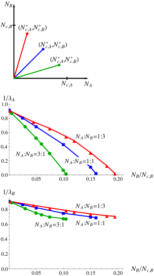
Figure 20: Demixing quantum transition of a binary cold BEC consisting of $A$- and $B$-atoms confined around the crossing of $\mathcal{C}$ assuming equal tube diameters $w_{x}^{\left(\mathcal{C}\right)}=w_{y}^{\left(\mathcal{C}\right)}=w_{z}^{\left(\mathcal{C}\right)}=2L$. Plots show the respective inverse localisation lengths $1/\lambda_{A}$ and $1/\lambda_{B}$ vs. particle number $N=N_{A}+N_{B}=(\frac{N_{A}}{N_{B}}+1)N_{B}$ for three different mixing ratios: red line $N_{A}:N_{B}=1:3$, blue line $N_{A}:N_{B}=1:1$, green line $N_{A}:N_{B}=3:1$. Mass ratio $\frac{m_{A}}{m_{B}}=\frac{87}{23}$ and interaction parameters $g_{AA}:g_{AB}:g_{BB}=1:1.7:2$ describe a binary BEC mixture consisting of ${}^{23}Na$- and ${}^{87}Rb$-atoms.

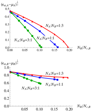
Figure 21: Chemical potentials $\mu_{A}$ and $\mu_{B}$ of a binary BEC mixture vs. particle number $N=N_{A}+N_{B}=(\frac{N_{A}}{N_{B}}+1)N_{B}$ assuming a fixed mixing ratio $N_{A}:N_{B}$. Here $\epsilon_{xt,B}=\varepsilon_{L}\times\frac{\pi^{2}}{2}$ and $\varepsilon_{xt,A}=\frac{m_{B}}{m_{A}}\varepsilon_{xt,B}$ denote the respective excitation thresholds for atoms with mass $m_{A}$ and $m_{B}$. Unit of length is $L$, unit of energy $\varepsilon_{L}=\frac{\hslash^{2}}{2m_{B}\ L^{2}}$. Mass and interaction parameters like in Fig.20.

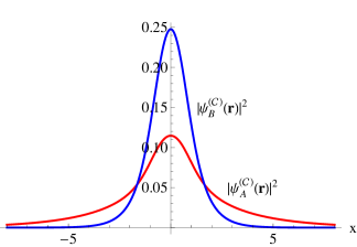
Figure 22: The profiles $|\psi_{A}^{(\mathcal{C})}(\mathbf{r})|^{2}$ and $|\psi_{B}^{(\mathcal{C})}(\mathbf{r})|^{2}$ along the axis $\mathbf{e}_{x}$ of the ground state GP-orbitals in a binary BEC mixture consisting of $A$- and $B$-atoms, assuming a mixing ratio $N_{A}:N_{B}=1:10$ and a filling fraction $N_{B}/N_{c,B}^{\star}=0.9$. Mass and interaction parameters like in Fig.20.

VII Conclusions

We have studied (within the range of validity of mean field theory) localised matter wave ground states of cold Bose atoms for different prototypes of quantum waveguides with broken translational symmetry: i) a waveguide system $\mathcal{C}$ akin to the shape of a swiss cross, ii) a waveguide $\mathcal{L}$ in the guise of a cranked $L$ with a rectangular corner, iii) a $T$-shaped waveguide $\mathcal{T}$ consisting of three branching arms, see Fig.1. The associated trapping mechanism is non standard, because the force confining the particles around the branching zone or crossing of waveguides cannot be derived from a potential.

Based on an analytic expression, that approximates for small propagation times $\Delta\tau$ the quantum propagator of a single particle at imaginary time, we solved numerically the three-dimensional Gross-Pitaevskii equation inside those quantum waveguides using a suitable splitting scheme, and found depending on the choice of the ratio $\kappa^{\left(\Gamma\right)}$ of lateral tube widths, for fixed particle number $N$, various localised Hartree ground states describing non standard trapping of cold interacting Bose atoms. The kernel representing the imaginary time quantum propagator implemented into the algorithm obeys by construction the Dirichlet boundary conditions at the walls $\partial\Gamma$ of the associated waveguides $\Gamma\in\left\{\mathcal{C},\mathcal{L},\mathcal{T}\right\}$ exactly.

Observing, that the transversal kinetic energy of a particle undergoes a rapid drop, when it traverses along a straight line the branching zone of the respective arms inside the waveguides $\Gamma$, we suggested an explanation for the existence of a localised ground state in section III. We also discussed the non existence of localised states in the waveguides $\Gamma$ for too small, respectively too large, lateral tube widths ratios $\kappa^{\left(\Gamma\right)}$, see Fig.7 and Fig.19. Analytical scaling laws obtained in section V for the dependence on $N$ of the localisation length $\lambda_{N}$ and the chemical potential $\mu_{N}$ agree very well with the results of the three-dimensional numerical calculations. We found that the kinetic energy of a BEC confined by this non standard trapping mechanism is by a factor seven(!) larger than the interaction energy, see Fig.15, so that the density profile of a BEC trapped around the branching or crossing zone of waveguides, see for example Fig.10 and Fig.22, cannot be described by the Thomas-Fermi approximation.

For the case of a binary mixture of two different Bose atom species $A$ and $B$ we observed non standard trapping of both atom species for subcritical particle numbers $N_{A}$ and $N_{B}$ around the branching or crossing zone of quantum waveguides. A sudden demixing quantum transition takes place at a critical particle number $N^{\star}=$ $N_{c,A}^{\star}+N_{c,B}^{\star}$ as the total particle number $N=N_{A}+N_{B}$ is increased at fixed mixing ratio $N_{A}/N_{B}$, see Fig. 20. Depending on the mass ratio $m_{A}/m_{B}$ the heavier atom species delocalises first for a wide range of interaction parameters. We found that in this case the dominant energy is not the interaction energy, but the kinetic energy of the atoms. This feature could perhaps be used to seperate isotopes.

Finally we mention, that the choice of a hard wall boundary condition (5) at the walls $\partial\Gamma$ of our waveguides $\Gamma\in\left\{\mathcal{C},\mathcal{L},\mathcal{T}\right\}$ serves in our calculations just as a convenient model. Choosing more general Robin boundary conditions (with a positive slip length), or replacing the walls of the tubes by a steep harmonic potential (which should be more appropriate to describe confinement generated by optical dipole forces) in no way changes qualitatively any of the above described localisation phenomena of cold matter waves around the branching or crossing zones of quantum waveguides.

Appendix A

The Magnus expansion theorem states for the product of the exponential of two linear operators $\hat{A}$ and $\hat{B}$ Wilcox

$$e^{\hat{A}}\circ e^{\hat{B}}=e^{\hat{A}+\hat{B}+\frac{1}{2}\left[\hat{A},\hat{B}\right]+\frac{1}{12}\left[\hat{A}-\hat{B},\left[\hat{A},\hat{B}\right]\right]+...}$$ (85)

, where $\left[\hat{A},\hat{B}\right]=\hat{A}\circ\hat{B}-\hat{B}\circ\hat{A}$. By explicit calculation, it can then be shown introducing a small parameter $\tau$:

$$\widehat{S}(\tau) = e^{-\frac{\tau}{2}\hat{A}}\circ e^{-\tau\hat{B}}\circ e^{-\frac{\tau}{2}\hat{A}}$$

$$= e^{-\tau\left(\hat{A}+\hat{B}\right)+\frac{\tau^{3}}{24}\left[\hat{A}+2\hat{B},\left[\hat{A},\hat{B}\right]\right]+O\left(\tau^{5}\right)...}$$

All even powers of $\ \tau$ in the exponent cancel as can be seen from the identity $\widehat{S}(\tau)\widehat{S}(-\tau)=\hat{1}$. There follows with real parameters $\lambda_{1}$, $\lambda_{2}>0$ :

$$\begin{array}[]{c}e^{-\lambda_{1}\tau\hat{B}}\circ e^{-\frac{\tau}{2}\hat{A}}\circ e^{-\lambda_{2}\tau\hat{B}}\circ e^{-\frac{\tau}{2}\hat{A}}\circ e^{-\lambda_{1}\tau\hat{B}}\\ \\ =\exp\left\{\begin{array}[]{c}-\left(2\lambda_{1}+\lambda_{2}\right)\tau\hat{B}\ -\tau\hat{A}\\ -\frac{\tau^{3}}{24}\left(4\lambda_{1}-\lambda_{2}\right)\left[\hat{A},\left[\hat{A},\hat{B}\right]_{-}\right]_{-}\\ -\frac{\tau^{3}}{24}\left(\left(\lambda_{1}+\lambda_{2}\right)4\lambda_{1}-2\lambda_{2}^{2}\right)\left[\hat{B},\left[\hat{B,}\hat{A}\right]_{-}\right]_{-}\\ +o\left(\tau^{5}\right)\end{array}\right\}\end{array}$$ (87)

Let us assume $||\hat{B}||\ll||\hat{A}||$. In order that equation (87) represents an accurate approximation to the original time development operator $e^{-\tau\left(\hat{A}+\hat{B}\right)}$ for small $\tau$ we require now $\lambda_{1}=\frac{1}{6}$ , $\lambda_{2}=\frac{2}{3}$. We consequently obtain that the accuracy of the approximation

$$e^{-\tau\left(\hat{A}+\hat{B}\right)}\simeq e^{-\frac{\tau}{6}\hat{B}}\circ e^{-\frac{\tau}{2}\hat{A}}\circ e^{-\frac{2\tau}{3}\hat{B}}\circ e^{-\frac{\tau}{2}\hat{A}}\circ e^{-\frac{\tau}{6}\hat{B}}$$ (88)

is of order $O\left(\tau^{2}||\hat{B}||^{2}+\tau^{4}||\hat{A}||^{4}\right)$. This property provides the basis of the splitting scheme as stated in (35).

Appendix B

It is convenient to write $w_{a}^{\left(\mathcal{C}\right)}=2L_{a}$ for the respective tube diameters $w_{a}^{\left(\mathcal{C}\right)}$ of the arms $\mathcal{A}_{j}\subset\mathcal{C}$, see Fig.1. One-dimensional heat kernels obeying to homogeneous Dirichlet boundary conditions at the end points of the intervals $\left[L_{a},\infty\right]$ , $\left[-\infty,-L_{a}\right]$ and $\left[-L_{a},L_{a}\right]$ may be found by the standard mirror method of Sommerfeld:

$$u,u^{\prime} \in \mathbb{R}$$ (89)

$$k(u-u^{\prime},\tau) = \frac{1}{\sqrt{4\pi\tau}}\exp\left[-\frac{(u-u^{\prime})^{2}}{4\tau}\right]$$

$$k_{[L_{a},\infty]}^{(D)}(u,u^{\prime};\tau) = k(u-u^{\prime};\tau)-k(u+u^{\prime}-2L_{a};\tau)$$

$$k_{[-\infty,-L_{a}]}^{(D)}(u,u^{\prime};\tau) = k(u-u^{\prime};\tau)-k(u+u^{\prime}+2L_{a};\tau)$$

$$k_{[-L_{a},L_{a}]}^{(D)}(u,u^{\prime};\tau) = \sum_{n\in\mathbb{Z}}\left[k(u-u^{\prime}+4nL_{a};\tau)\right.$$

$$\left.-k(u+u^{\prime}+(4n+2)L_{a};\tau)\right]$$

We show in Supplementary Material , that the short time expansion of the three-dimensional imaginary time quantum propagator $K(\mathbf{r},\mathbf{r}^{\prime};\Delta\tau)=\left\langle\mathbf{r}\right|e^{-\Delta\tau H_{kin}}\left|\mathbf{r}^{\prime}\right\rangle$ obeying to Dirichlet boundary conditions at the walls $\partial\mathcal{C}$ of a cross shaped waveguide $\mathcal{C}$, assumes for a small diffusion time $\Delta\tau>0$ the following explicit guise:

$$\left[K(\mathbf{r},\mathbf{r}^{\prime};\Delta\tau)\right]_{\mathbf{r}\in\mathcal{A}_{j},\mathbf{r}^{\prime}\in\mathcal{A}_{l}}=\mathcal{K}_{\mathcal{A}_{j},\mathcal{A}_{l}}\left(\mathbf{r},\mathbf{r}^{\prime};\Delta\tau\right)=\mathcal{K}_{\mathcal{A}_{j},\mathcal{A}_{l}}^{\left(\perp\right)}\left(\mathbf{r}_{\perp},\mathbf{r}_{\perp}^{\prime};\Delta\tau\right)k_{[-L_{z},L_{z}]}^{\left(D\right)}(z,z^{\prime};\Delta\tau)$$ (90)

$$\mathcal{K}_{\mathcal{A}_{0},\mathcal{A}_{0}}^{\left(\perp\right)}\left(\mathbf{r}_{\perp},\mathbf{r}_{\perp}^{\prime};\Delta\tau\right)=\left[\begin{array}[]{c}k_{[-L_{x},L_{x}]}^{\left(D\right)}(x,x^{\prime};\Delta\tau)k_{[-L_{y},L_{y}]}^{\left(D\right)}(y,y^{\prime};\Delta\tau)\\ \\ +\left[C_{\mathcal{A}_{3},\mathcal{A}_{0}}(x,x^{\prime};\Delta\tau)-C_{\mathcal{A}_{1},\mathcal{A}_{0}}(x,x^{\prime};\Delta\tau)\right]k_{[-L_{y},L_{y}]}^{\left(D\right)}(y,y^{\prime};\Delta\tau)\\ \\ +k_{[-L_{x},L_{x}]}^{\left(D\right)}(x,x^{\prime};\Delta\tau)\left[C_{\mathcal{A}_{4},\mathcal{A}_{0}}(y,y^{\prime};\Delta\tau)-C_{\mathcal{A}_{2},\mathcal{A}_{0}}(y,y^{\prime};\Delta\tau)\right]\end{array}\right]$$

$$\mathcal{K}_{\mathcal{A}_{0},\mathcal{A}_{1}}^{\left(\perp\right)}\left(\mathbf{r}_{\perp},\mathbf{r}_{\perp}^{\prime};\Delta\tau\right) = C_{\mathcal{A}_{1},\mathcal{A}_{1}}(x,x^{\prime};\Delta\tau)k_{[-L_{y},L_{y}]}^{\left(D\right)}(y,y^{\prime};\Delta\tau)$$

$$\mathcal{K}_{\mathcal{A}_{0},\mathcal{A}_{2}}^{\left(\perp\right)}\left(\mathbf{r}_{\perp},\mathbf{r}_{\perp}^{\prime};\Delta\tau\right) = k_{[-L_{x},L_{x}]}^{\left(D\right)}(x,x^{\prime};\Delta\tau)C_{\mathcal{A}_{2},\mathcal{A}_{2}}(y,y^{\prime};\Delta\tau)$$

$$\mathcal{K}_{\mathcal{A}_{0},\mathcal{A}_{3}}^{\left(\perp\right)}\left(\mathbf{r}_{\perp},\mathbf{r}_{\perp}^{\prime};\Delta\tau\right) = -C_{\mathcal{A}_{3},\mathcal{A}_{3}}(x,x^{\prime};\Delta\tau)k_{[-L_{y},L_{y}]}^{\left(D\right)}(y,y^{\prime};\Delta\tau)$$

$$\mathcal{K}_{\mathcal{A}_{0},\mathcal{A}_{4}}^{\left(\perp\right)}\left(\mathbf{r}_{\perp},\mathbf{r}_{\perp}^{\prime};\Delta\tau\right) = -k_{[-L_{x},L_{x}]}^{\left(D\right)}(x,x^{\prime};\Delta\tau)C_{\mathcal{A}_{4},\mathcal{A}_{4}}(y,y^{\prime};\Delta\tau)$$

$$\mathcal{K}_{\mathcal{A}_{1},\mathcal{A}_{0}}^{\left(\perp\right)}\left(\mathbf{r}_{\perp},\mathbf{r}_{\perp}^{\prime};\Delta\tau\right) = \left[C_{\mathcal{A}_{3},\mathcal{A}_{0}}(x,x^{\prime};\Delta\tau)-C_{\mathcal{A}_{1},\mathcal{A}_{0}}(x,x^{\prime};\Delta\tau)\right]k_{[-L_{y},L_{y}]}^{\left(D\right)}(y,y^{\prime};\Delta\tau)$$

$$\mathcal{K}_{\mathcal{A}_{1},\mathcal{A}_{1}}^{\left(\perp\right)}\left(\mathbf{r}_{\perp},\mathbf{r}_{\perp}^{\prime};\Delta\tau\right) = \left[k_{[L_{x},\infty]}^{\left(D\right)}(x,x^{\prime};\Delta\tau)+C_{\mathcal{A}_{1},\mathcal{A}_{1}}(x,x^{\prime};\Delta\tau)\right]k_{[-L_{y},L_{y}]}^{\left(D\right)}(y,y^{\prime};\Delta\tau)$$

$$\mathcal{K}_{\mathcal{A}_{1},\mathcal{A}_{2}}^{\left(\perp\right)}\left(\mathbf{r}_{\perp},\mathbf{r}_{\perp}^{\prime};\Delta\tau\right) = 0=\mathcal{K}_{\mathcal{A}_{1},\mathcal{A}_{4}}^{\left(\perp\right)}\left(\mathbf{r}_{\perp},\mathbf{r}_{\perp}^{\prime};\Delta\tau\right)$$

$$\mathcal{K}_{\mathcal{A}_{1},\mathcal{A}_{3}}^{\left(\perp\right)}\left(\mathbf{r}_{\perp},\mathbf{r}_{\perp}^{\prime};\Delta\tau\right) = -C_{\mathcal{A}_{3},\mathcal{A}_{3}}(x,x^{\prime};\Delta\tau)k_{[-L_{y},L_{y}]}^{\left(D\right)}(y,y^{\prime};\Delta\tau)$$

$$\mathcal{K}_{\mathcal{A}_{2},\mathcal{A}_{0}}^{\left(\perp\right)}\left(\mathbf{r}_{\perp},\mathbf{r}_{\perp}^{\prime};\Delta\tau\right) = k_{[-L_{x},L_{x}]}^{\left(D\right)}(x,x^{\prime};\Delta\tau)\left[C_{\mathcal{A}_{4},\mathcal{A}_{0}}(y,y^{\prime};\Delta\tau)-C_{\mathcal{A}_{2},\mathcal{A}_{0}}(y,y^{\prime};\Delta\tau)\right]$$

$$\mathcal{K}_{\mathcal{A}_{2},\mathcal{A}_{1}}^{\left(\perp\right)}\left(\mathbf{r}_{\perp},\mathbf{r}_{\perp}^{\prime};\Delta\tau\right) = 0=\mathcal{K}_{\mathcal{A}_{2},\mathcal{A}_{3}}^{\left(\perp\right)}\left(\mathbf{r}_{\perp},\mathbf{r}_{\perp}^{\prime};\Delta\tau\right)$$

$$\mathcal{K}_{\mathcal{A}_{2},\mathcal{A}_{2}}^{\left(\perp\right)}\left(\mathbf{r}_{\perp},\mathbf{r}_{\perp}^{\prime};\Delta\tau\right) = k_{[-L_{x},L_{x}]}^{\left(D\right)}(x,x^{\prime};\Delta\tau)\left[k_{[L_{y},\infty]}^{\left(D\right)}(y,y^{\prime};\Delta\tau)+C_{\mathcal{A}_{2},\mathcal{A}_{2}}(y,y^{\prime};\Delta\tau)\right]$$

$$\mathcal{K}_{\mathcal{A}_{2},\mathcal{A}_{4}}^{\left(\perp\right)}\left(\mathbf{r}_{\perp},\mathbf{r}_{\perp}^{\prime};\Delta\tau\right) = -k_{[-L_{x},L_{x}]}^{\left(D\right)}(x,x^{\prime};\Delta\tau)C_{\mathcal{A}_{4},\mathcal{A}_{4}}(y,y^{\prime};\Delta\tau)$$

$$\mathcal{K}_{\mathcal{A}_{3},\mathcal{A}_{0}}^{\left(\perp\right)}\left(\mathbf{r}_{\perp},\mathbf{r}_{\perp}^{\prime};\Delta\tau\right) = \left[C_{\mathcal{A}_{3},\mathcal{A}_{0}}(x,x^{\prime};\Delta\tau)-C_{\mathcal{A}_{1},\mathcal{A}_{0}}(x,x^{\prime};\Delta\tau)\right]k_{[-L_{y},L_{y}]}^{\left(D\right)}(y,y^{\prime};\Delta\tau)$$

$$\mathcal{K}_{\mathcal{A}_{3},\mathcal{A}_{1}}^{\left(\perp\right)}\left(\mathbf{r}_{\perp},\mathbf{r}_{\perp}^{\prime};\Delta\tau\right) = C_{\mathcal{A}_{1},\mathcal{A}_{1}}(x,x^{\prime};\Delta\tau)k_{[-L_{y},L_{y}]}^{\left(D\right)}(y,y^{\prime};\Delta\tau)$$

$$\mathcal{K}_{\mathcal{A}_{3},\mathcal{A}_{2}}^{\left(\perp\right)}\left(\mathbf{r}_{\perp},\mathbf{r}_{\perp}^{\prime};\Delta\tau\right) = 0=\mathcal{K}_{\mathcal{A}_{3},\mathcal{A}_{4}}^{\left(\perp\right)}\left(\mathbf{r}_{\perp},\mathbf{r}_{\perp}^{\prime};\Delta\tau\right)$$

$$\mathcal{K}_{\mathcal{A}_{3},\mathcal{A}_{3}}^{\left(\perp\right)}\left(\mathbf{r}_{\perp},\mathbf{r}_{\perp}^{\prime};\Delta\tau\right) = \left[k_{[-\infty,-L_{x}]}^{\left(D\right)}(x,x^{\prime};\Delta\tau)-C_{\mathcal{A}_{3},\mathcal{A}_{3}}(x,x^{\prime};\Delta\tau)\right]k_{[-L_{y},L_{y}]}^{\left(D\right)}(y,y^{\prime};\Delta\tau)$$

$$\mathcal{K}_{\mathcal{A}_{4},\mathcal{A}_{0}}^{\left(\perp\right)}\left(\mathbf{r}_{\perp},\mathbf{r}_{\perp}^{\prime};\Delta\tau\right) = k_{[-L_{x},L_{x}]}^{\left(D\right)}(x,x^{\prime};\Delta\tau)\left[C_{\mathcal{A}_{4},\mathcal{A}_{0}}(y,y^{\prime};\Delta\tau)-C_{\mathcal{A}_{2},\mathcal{A}_{0}}(y,y^{\prime};\Delta\tau)\right]$$

$$\mathcal{K}_{\mathcal{A}_{4},\mathcal{A}_{1}}^{\left(\perp\right)}\left(\mathbf{r}_{\perp},\mathbf{r}_{\perp}^{\prime};\Delta\tau\right) = 0=\mathcal{K}_{\mathcal{A}_{4},\mathcal{A}_{3}}^{\left(\perp\right)}\left(\mathbf{r}_{\perp},\mathbf{r}_{\perp}^{\prime};\Delta\tau\right)$$

$$\mathcal{K}_{\mathcal{A}_{4},\mathcal{A}_{2}}^{\left(\perp\right)}\left(\mathbf{r}_{\perp},\mathbf{r}_{\perp}^{\prime};\Delta\tau\right) = k_{[-L_{x},L_{x}]}^{\left(D\right)}(x,x^{\prime};\Delta\tau)C_{\mathcal{A}_{2},\mathcal{A}_{2}}(y,y^{\prime};\Delta\tau)$$

$$\mathcal{K}_{\mathcal{A}_{4},\mathcal{A}_{4}}^{\left(\perp\right)}\left(\mathbf{r}_{\perp},\mathbf{r}_{\perp}^{\prime};\Delta\tau\right) = k_{[-L_{x},L_{x}]}^{\left(D\right)}(x,x^{\prime};\Delta\tau)\left[k_{[-\infty,-L_{y}]}^{\left(D\right)}(y,y^{\prime};\Delta\tau)-C_{\mathcal{A}_{4},\mathcal{A}_{4}}(y,y^{\prime};\Delta\tau)\right]$$

$$C_{\mathcal{A}_{1},\mathcal{A}_{0}}(x,x^{\prime};\tau) = \sum_{n=-\infty}^{\infty}\textnormal{sgn}\left[\ x^{\prime}-\left(4n+1\right)L_{x}\right]k(\left|x-L_{x}\right|+\ \left|x^{\prime}-\left(4n+1\right)L_{x}\right|;\tau)$$ (91)

$$C_{\mathcal{A}_{2},\mathcal{A}_{0}}(y,y^{\prime};\tau) = \sum_{n=-\infty}^{\infty}\textnormal{sgn}\left[\ y^{\prime}-\left(4n+1\right)L_{y}\right]k(\left|y-L_{y}\right|+\ \left|y^{\prime}-\left(4n+1\right)L_{y}\right|;\tau)$$

$$C_{\mathcal{A}_{1},\mathcal{A}_{1}}(x,x^{\prime};\tau) = \textnormal{sgn}\left(x^{\prime}-L_{x}\right)k(\left|x-L_{x}\right|+\left|x^{\prime}-L_{x}\right|;\tau)$$

$$C_{\mathcal{A}_{2},\mathcal{A}_{2}}(y,y^{\prime};\tau) = \textnormal{sgn}\left(y^{\prime}-L_{y}\right)k(\left|y-L_{y}\right|+\left|y^{\prime}-L_{y}\right|;\tau)$$

$$C_{\mathcal{A}_{3},\mathcal{A}_{0}}(x,x^{\prime};\tau) = \sum_{n=-\infty}^{\infty}\textnormal{sgn}\left[x^{\prime}+\left(4n+1\right)L_{x}\right]k(\left|x+L_{x}\right|+\left|x^{\prime}+\left(4n+1\right)L_{x}\right|;\tau)$$

$$C_{\mathcal{A}_{4},\mathcal{A}_{0}}(y,y^{\prime};\tau) = \sum_{n=-\infty}^{\infty}\textnormal{sgn}\left[y^{\prime}+\left(4n+1\right)L_{y}\right]k(\left|y+L_{y}\right|+\left|y^{\prime}+\left(4n+1\right)L_{y}\right|;\tau)$$

$$C_{\mathcal{A}_{3},\mathcal{A}_{3}}(x,x^{\prime};\tau) = \textnormal{sgn}\left(x^{\prime}+L_{x}\right)k(\left|x+L_{x}\right|+\left|x^{\prime}+L_{x}\right|;\tau)$$

$$C_{\mathcal{A}_{4},\mathcal{A}_{4}}(y,y^{\prime};\tau) = \textnormal{sgn}\left(y^{\prime}+L_{y}\right)k(\left|y+L_{y}\right|+\left|y^{\prime}+L_{y}\right|;\tau)$$

References

- (1) Y.P. Feng, C.F. Majkrzak, S.K. Sinha, D.G. Wieserl, H. Zhang, and H.W. Deckman, Phys. Rev. B 49, 10814 (1994).
- (2) S.P. Pogossian, A. Menelle, H. LeGall, J. Ben-Youssef, and J.M. Desvignes, J. Appl. Phys. 83, 1159 (1997).
- (3) M.J. Renn, D. Montgomery, O. Vdovin, D.Z. Anderson, C.E. Wieman, and E.A. Cornell, Phys. Rev. Lett. 75, 3253 (1995).
- (4) H. Ito, T. Nakata, K. Sakaki, M. Ohtsu, K.I. Lee and W. Jhe, Phys. Rev. Lett. 76, 4500 (1996).
- (5) D. Mueller, E.A. Cornell, D.Z. Anderson, and E.R.I. Abraham Phys. Rev. A 61, 033411 (2000).
- (6) C.A. Christensen, S. Will, M. Saba, G. Jo, Y. Shin, W. Ketterle and D. Pritchard, Phys. Rev. A 78, 033429 (2008).
- (7) S. Vorrath, S.A. Möller, P. Windpassinger, K. Bongs and K. Sengstock, New Journal of Physics 12, 123015 (2010).
- (8) J.A. Pechkis and F.K. Fatemi, Optics Express 20, 13409 (2012).
- (9) A.H. Barnett, S.P. Smith, M. Olshanii, K.S. Johnson, A.W. Adams, and P. Prentiss, Phys. Rev. A 61, 023608 (2000).
- (10) F.L. Kien, V.I. Balykin, and K. Hakuta, Phys. Rev. A 70, 063403 (2004).
- (11) K.P. Nayak, P.N. Melentiev, M. Morinaga, F.L. Kien, V.I. Balykin, and K. Hakuta, Optics Express 15, 5431 (2007).
- (12) E. Vetsch, D. Reitz, G. Sagué, R. Schmidt, S.T. Dawkins and A. Rauschenbeutel, Phys. Rev. Lett. 104, 203603 (2010).
- (13) L. Stern, B. Desiatov, I. Goykhman, and U. Levy, Nature Com. 4, 1548 (2013)
- (14) M. Schiffer, M. Rauner, S. Kuppens, M. Zinner, K. Sengstock, and W. Ertmer, Appl. Phys. B 67, 705 (1998).
- (15) A. Jaouadi, N. Gaaloul, B. Viaris de Lesegno, M. Telmini, L. Pruvost, and E. Charron, Phys. Rev. A 82, 023613 (2010).
- (16) R.L. Schult , D.G. Ravenhall, and H.W. Wyld, Phys. Rev. B 39, 5476 (1989).
- (17) P. Exner and V.A. Zagrebnov, J. Phys. A 38, L463 (2005).
- (18) P. Exner and P. Seba, J. Math. Phys. 30, 2574 (1989).
- (19) P. Duclos and D. Exner, Rev. Math. Phys. 7, 73 (1995).
- (20) M.W.J. Bromley and B.D. Esry, Phys. Rev. A 68, 043609 (2003).
- (21) Y. Avishai, D. Bessis, B.G. Giraud, and G. Mantica, Phys. Rev. B 44, 8028 (1991).
- (22) E. Sadourni and W.P. Schleich, AIP Conf.Proc. 1323, 283 (2010).
- (23) S.A. Nazarov, Acoustical Physics 56, 1004 (2010).
- (24) M. Dauge, Y. Lafranche, and N. Raymond, ESAIM: Proc. 35, 14 (2012).
- (25) J. Goldstone and R.L. Jaffe, Phys. Rev. B 45, 14100 (1992).
- (26) P. Leboeuf and N. Pavloff, Phys. Rev. A 64, 033602 (2001).
- (27) D. Borisov, P. Exner, and A. Golovina, arXiv: 1210.0449 [math-phys].
- (28) A.L. Delitsyn , B.T. Nguyen, and D.S. Grebenkov, Eur. Phys. J. B 85, 176 (2012).
- (29) L.N. Trefethen, Approximation Theory and Approximation Praxis, SIAM (2013).
- (30) M. de Gosson and B.Hiley, Phys. Lett. A 377 (42), 3005 (2013).
- (31) P. Exner, P. Seba, and P. Stovicek, Czech. J. Phys. B 39, 181 (1989).
- (32) P. Amore, M. Rodriguez, and C.A. Terreo-Escalante, J. Phys. A 45, 105303 (2012).
- (33) L.N. Trefethen and T. Betcke, Computed eigenmodes of planar regions, Contemporary Mathematics (2005).
- (34) S.A. Nazarov and A.V. Shanin, Computational Mathematics and Computational Physics 51, 96 (2011).
- (35) A.L. Delitsyn , B.T. Nguyen, and D.S. Grebenkov, Eur. Phys. J. B 85, 371 (2012).
- (36) G. Baym, ”Lectures on Quantum Mechanics” , 6th ed. (Benjamin, 1978).
- (37) S.A. Chin and E. Krotscheck, Physical Review E 72, 036705 (2005).
- (38) C.J. Pethick and H. Smith, Bose-Einstein Condensation in Dilute Gases, 2nd ed. (Cambridge University Press, New York, 2008).
- (39) D. Xiong, X. Li, F. Wang, and D. Wang et al, arXiv: 1305.7091 (2013).
- (40) R.M. Wilcox, J. Math. Phys. 8, 962 (1967).
- (41) J.P. Martikainen, Phys. Rev. A 63, 043602 (2001).
- (42) A. Markowsky and N. Schopohl, ”Supplemental material to: Cold Bose Atoms Around the Crossing of a Quantum Waveguide”, (submitted to Phys. Rev. A).