Thermal Density Functional Theory in Context

I Abstract

This chapter introduces thermal density functional theory, starting from the ground-state theory and assuming a background in quantum mechanics and statistical mechanics. We review the foundations of density functional theory (DFT) by illustrating some of its key reformulations. The basics of DFT for thermal ensembles are explained in this context, as are tools useful for analysis and development of approximations. We close by discussing some key ideas relating thermal DFT and the ground state. This review emphasizes thermal DFT’s strengths as a consistent and general framework.

II Introduction

The subject matter of high-energy-density physics is vast HEDP03 , and the various methods for modeling it are diverse MD06 ; GBBC12 ; STVM00 . The field includes enormous temperature, pressure, and density ranges, reaching regimes where the tools of plasma physics are appropriate A04 . But, especially nowadays, interest also stretches down to warm dense matter (WDM), where chemical details can become not just relevant, but vital KD09 . WDM, in turn, is sufficiently close to zero-temperature, ground-state electronic structure that the methods from that field, especially Kohn-Sham density functional theory (KS DFT) KRDM08 ; RMCH10 , provide a standard paradigm for calculating material-specific properties with useful accuracy.

It is important to understand, from the outset, that the logic and methodology of KS-DFT is at times foreign to other techniques of theoretical physics. The procedures of KS-DFT appear simple, yet the underlying theory is surprisingly subtle. Consequently, progress in developing useful approximations, or even writing down formally correct expressions, has been incredibly slow. As the KS methodology develops in WDM and beyond, it is worth taking a few moments to wrap one’s head around its logic, as it does lead to one of the most successful paradigms of modern electronic structure theory B12 .

This chapter sketches how the methodology of KS DFT can be generalized to warm systems, and what new features are introduced in doing so. It is primarily designed for those unfamiliar with DFT to get a general understanding of how it functions and what promises it holds in the domain of warm dense matter. Section 2 is a general review of the basic theorems of DFT, using the original methodology of Hohenberg-Kohn HK64 and then the more general Levy-Lieb construction L79 ; L83 . In Section 3, we discuss approximations, which are always necessary in practice, and several important exact conditions that are used to guide their construction. In Section 4, we review the thermal KS equations M65 and some relevant statistical mechanics. Section 5 summarizes some of the most important exact conditions for thermal ensembles PPFS11 ; DT11 . Last, but not least, in Section 6 we review some recent results that generalize ground-state exact scaling conditions and note some of the main differences between the finite-temperature and the ground-state formulation.

III Density functional theory

A reformulation of the interacting many-electron problem in terms of the electron density rather than the many-electron wavefunction has been attempted since the early days of quantum mechanics T27 ; F27 ; F28 . The advantage is clear: while the wavefunction for interacting electrons depends in a complex fashion on all the particle coordinates, the particle density is a function of only three spatial coordinates.

Initially, it was believed that formulating quantum mechanics solely in terms of the particle density gives only an approximate solution, as in the Thomas-Fermi method T27 ; F27 ; F28 . However, in the mid-1960s, Hohenberg and Kohn HK64 showed that, for systems of electrons in an external potential, all the properties of the many-electron ground state are, in principle, exactly determined by the ground-state particle density alone.

Another important approach to the many-particle problem appeared early in the development of quantum mechanics: the single-particle approximation. Here, the two-particle potential representing the interaction between particles is replaced by some effective, one-particle potential. A prominent example of this approach is the Hartree-Fock method F30 ; H35 , which includes only exchange contributions in its effective one-particle potential. A year after the Hohenberg-Kohn theorem had been proven, Kohn and Sham KS65 took a giant leap forward. They took the ground state particle density as the basic quantity and showed that both exchange and correlation effects due to the electron-electron interaction can be treated through an effective single-particle Schrödinger equation. Although Kohn and Sham wrote their paper using the local density approximation, they also pointed out the exactness of that scheme if the exact exchange-correlation functional were to be used (see Section III.3). The KS scheme is used in almost all DFT calculations of electronic structure today. Much development in this field remains focused on improving approximations to the exchange-correlation energy (see Section IV).

The Hohenberg-Kohn theorem and Kohn-Sham scheme are the basic elements of modern density-functional theory (DFT) B12 ; B07 ; BW13 . We will review the initial formulation of DFT for non-degenerate ground states and its later extension to degenerate ground states. Alternative and refined mathematical formulations are then introduced.

III.1 Introduction

The non-relativistic Hamiltonian for $N$ interacting electrons moving in a static potential $v({\bf r})$ reads (in atomic units)

$$\hat{H}=\hat{T}+\hat{V}_{ee}+\hat{V}:=-\frac{1}{2}\sum_{i=1}^{N}\nabla^{2}_{i}+\frac{1}{2}\sum_{\stackrel{{\scriptstyle i,j=1}}{{i\neq j}}}^{N}\frac{1}{|{\bf r}_{i}-{\bf r}_{j}|}+\sum_{i=1}^{N}v({\bf r}_{i}).$$ (1)

Here, $\hat{T}$ is the total kinetic-energy operator, $\hat{V}_{ee}$ describes the repulsion between the electrons, and $\hat{V}$ is a local (multiplicative) scalar operator. This includes the interaction of the electrons with the nuclei (considered within the Born-Oppenheimer approximation) and any other external scalar potentials.

The eigenstates, $\Psi_{i}({\bf r}_{1},...,{\bf r}_{N})$, of the system are obtained by solving the eigenvalue problem

$$\hat{H}\Psi_{i}({\bf r}_{1},...,{\bf r}_{N})=E_{i}\Psi_{i}({\bf r}_{1},...,{\bf r}_{N}),$$ (2)

with appropriate boundary conditions for the physical problem at hand. Eq. (2) is the time-independent Schrödinger equation. We are particularly interested in the ground state, the eigenstate with lowest energy, and assume the wavefunction can be normalized.

Due to the interactions among the electrons, $\hat{V}_{ee}$, an explicit and closed solution of the many-electron problem in Eq. (2) is, in general, not possible. But because accurate prediction of a wide range of physical and chemical phenomena requires inclusion of electron-electron interaction, we need a path to accurate approximate solutions.

Once the number of electrons with Coulombic interaction is given, the Hamiltonian is determined by specifying the external potential. For a given $v({\bf r})$, the total energy is a functional of the many-body wavefunction $\Psi({\bf r}_{1},...,{\bf r}_{N})$

$$E_{v}[\Psi]=\langle\Psi|\hat{T}+\hat{V}_{ee}+\hat{V}|\Psi\rangle\;.$$ (3)

The energy functional in Eq. (3) may be evaluated for any $N$-electron wavefunction, and the Rayleigh-Ritz variational principle ensures that the ground state energy, $E_{v}$, is given by

$$E_{v}=\inf_{\Psi}E_{v}[\Psi],$$ (4)

where the infimum is taken over all normalized, antisymmetric wavefunctions. The Euler-Lagrange equation expressing the minimization of the energy is

$$\frac{\delta}{\delta\Psi}\left\{E_{v}[\Psi]-\mu\left[\langle\Psi|\Psi\rangle-1\right]\right\}=0,$$ (5)

where the functional derivative is performed over $\Psi\in{\cal L}^{2}(\mathbb{R}^{3N})$ (defined as in Ref. ED11 ). Relation (5) again leads to the many-body Schrödinger equation and the Lagrangian multiplier $\mu$ can be identified as the chemical potential.

We now have a procedure for finding approximate solutions by restricting the form of the wavefunctions. In the Hartree-Fock (HF) approximation, for example, the form of the wave-function is restricted to a single Slater determinant. Building on the HF wavefunction, modern quantum chemical methods can produce extremely accurate solutions to the Schrödinger equation S10 . Unfortunately, wavefunction-based approaches that go beyond HF usually are afflicted by an impractical growth of the numerical effort with the number of particles. Inspired by the Thomas-Fermi approach, one might wonder if the role played by the wavefunction could be played by the particle density, defined as

$$n({\bf r}) :=\langle\Psi|\sum_{i=1}^{N}\delta({\bf\hat{r}}-{\bf\hat{r}}_{i})|\Psi\rangle$$

$$=N\int d{\bf r}_{2}...\int d{\bf r}_{N}\Big{|}\Psi({\bf r},{\bf r}_{2},...,{\bf r}_{N})\Big{|}^{2},$$ (6)

from which

$$\int{d^{3}r}~{}n({\bf r})=N.$$ (7)

In that case, one would deal with a function of only three spatial coordinates, regardless of the number of electrons.

III.2 Hohenberg-Kohn theorem

Happily, the two-part Hohenberg-Kohn (HK) Theorem assures us that the electronic density alone is enough to determine all observable quantities of the systems. These proofs cleverly connect specific sets of densities, wavefunctions, and potentials, exposing a new framework for the interacting many-body problem.

Let $\bf{P}$ be the set of external potentials leading to a non-degenerate ground state for $N$ electrons. For a given potential, the corresponding ground state, $\Psi$, is obtained through the solution of the Schrödinger equation:

$$v~{}~{}\longrightarrow~{}~{}\Psi,~{}~{}\mbox{with}~{}~{}v\in\bf{P}.$$ (8)

Wavefunctions obtained this way are called interacting v-representable. We collect these ground state wavefunctions in the set $\bf{W}$. The corresponding particle densities can be computed using definition (III.1):

$$\Psi~{}~{}\longrightarrow~{}~{}n,~{}~{}\mbox{with}~{}~{}\Psi\in\bf{W}.$$ (9)

Ground state particle densities obtained this way are also called interacting v-representable. We denote the set of these densities as $\bf{D}$.

III.2.1 First part

Given a density $n\in\bf{D}$, the first part of the Hohenberg-Kohn theorem states that the wavefunction $\Psi\in\bf{W}$ leading to $n$ is unique, apart from a constant phase factor. The proof is carried out by reductio ad absurdum and is illustrated in Figure 1.

Figure 1: The Hohenberg-Kohn proves the one-to-one mappings between potentials and ground-state wavefunctions and between ground-state wavefunctions and ground-state densities. The dotted lines indicated by question marks show the two-to-one mappings disproved by Hohenberg and Kohn ED11 ; DG90 .

Consider two different wavefunctions in $\bf{W}$, $\Psi_{1}$ and $\Psi_{2}$, that differ by more than a constant phase factor. Next, let $n_{1}$ and $n_{2}$ be the corresponding densities computed by Eq. (III.1). Since, by construction, we are restricting ourselves to non-degenerate ground states, $\Psi_{1}$ and $\Psi_{2}$ must come from two different potentials. Name these $v_{1}$ and $v_{2}$, respectively.

Assume that these different wavefunctions yield the same density:

$$\Psi_{1}\neq\Psi_{2}~{}~{}\mbox{but}~{}~{}n_{1}({\bf r})=n_{2}({\bf r}).$$ (10)

Application of the Rayleigh-Ritz variational principle yields the inequality

$$\langle\Psi_{1}|\hat{H}_{1}|\Psi_{1}\rangle<\langle\Psi_{2}|\hat{H}_{1}|\Psi_{2}\rangle,$$ (11)

from which we obtain

$$E_{1}<\langle\Psi_{2}|\hat{H}_{2}+(\hat{V}_{1}-\hat{V}_{2})|\Psi_{2}\rangle=E_{2}+\int{d^{3}r}~{}n_{1}({\bf r})\left[v_{1}({\bf r})-v_{2}({\bf r})\right].$$ (12)

Reversing the role of systems 1 and 2 in the derivation, we find

$$E_{2}<\langle\Psi_{1}|\hat{H}_{1}+(\hat{V}_{2}-\hat{V}_{1})|\Psi_{1}\rangle=E_{1}+\int{d^{3}r}~{}n_{2}({\bf r})\left[v_{2}({\bf r})-v_{1}({\bf r})\right].$$ (13)

The assumption that the two densities are equal, $n_{1}({\bf r})=n_{2}({\bf r})$, and addition of the inequalities (12) and (13) yields

$$E_{1}+E_{2}<E_{1}+E_{2},$$ (14)

which is a contradiction. We conclude that the foregoing hypothesis (10) was wrong, so $n_{1}\neq n_{2}$. Thus each density is the ground-state density of, at most, one wavefunction. This mapping between the density and wavefunction is written

$$n~{}\longrightarrow~{}\Psi,~{}\mbox{with}~{}n\in{\bf D}~{}\mbox{and}~{}\Psi\in\bf{W}.$$ (15)

III.2.2 Second part

Having specified the correspondence between density and wavefunction, Hohenberg and Kohn then consider the potential. By explicitly inverting the Schrödinger equation,

$$\sum_{i=1}^{N}v({\bf r}_{i})=E-\frac{\left(\hat{T}+\hat{V}_{ee}\right)\Psi({\bf r}_{1},{\bf r}_{2},...,{\bf r}_{N})}{\Psi({\bf r}_{1},{\bf r}_{2},...,{\bf r}_{N})},$$ (16)

they show the elements $\Psi$ of $\bf{W}$ also determine the elements $v$ of $\bf{P}$, apart from an additive constant.

We summarize this second result by writing

$$\Psi~{}\longrightarrow~{}v,~{}\mbox{with}~{}\Psi\in{\bf W}~{}\mbox{and}~{}v\in\bf{P}.$$ (17)

III.2.3 Consequences

Together, the first and second parts of the theorem yield

$$n\longrightarrow v+const,~{}~{}\mbox{with}~{}n\in{\bf D}~{}\mbox{and}~{}v\in\bf{P},$$ (18)

that the ground state particle density determines the external potential up to a trivial additive constant. This is the first HK theorem.

Moreover, from the first part of the theorem it follows that any ground-state observable is a functional of the ground-state particle density. Using the one-to-one dependence of the wavefunction, $\Psi[n]$, on the particle density,

$$\langle\Psi|\hat{O}|\Psi\rangle=\langle\Psi[n]|\hat{O}|\Psi[n]\rangle=O[n].$$ (19)

For example, the following functional can be defined:

$$E_{v,\rm HK}[n] :=\langle\Psi[n]|\hat{T}+\hat{V}_{ee}+\hat{V}|\Psi[n]\rangle$$

$$=F_{\rm HK}[n]+\int{d^{3}r}~{}n({\bf r})v({\bf r}),$$ (20)

where $v$ is a given external potential and $n$ can be any density in $\bf{D}$. Note that

$$F_{\rm HK}[n]:=\langle\Psi[n]|\hat{T}+\hat{V}_{ee}|\Psi[n]\rangle$$ (21)

is independent of $v$. The second HK theorem is simply that $F_{\rm HK}[n]$ is independent of $v({\bf r})$. This is therefore a universal functional of the ground-state particle density. We use the subscript, ${\rm HK}$, to emphasize that this is the original density functional of Hohenberg and Kohn.

Let $n_{0}$ be the ground-state particle density of the potential $v_{0}$. The Rayleigh-Ritz variational principle (4) immediately tells us

$$E_{v_{0}}=\min_{n\in\bf{D}}E_{v_{0},\rm HK}[n]=E_{v_{0},\rm HK}[n_{0}].$$ (22)

We have finally obtained a variational principle based on the particle density instead of the computationally expensive wavefunction.

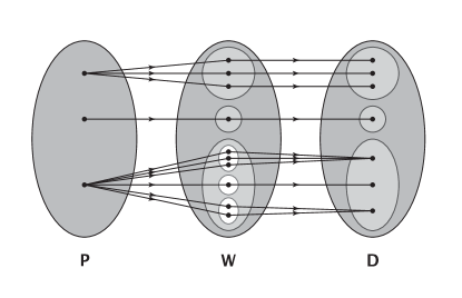
III.2.4 Extension to degenerate ground states

The Hohenberg-Kohn theorem can be generalized by allowing $\bf{P}$ to include local potentials having degenerate ground states L79 ; Kohn:85 ; DG90 , . This means an entire subspace of wavefunctions can correspond to the lowest eigenvalue of the Schrödinger equation (2). The sets $\bf{W}$ and $\bf{D}$ are enlarged accordingly, to include all the additional ground-state wavefunctions and particle densities.

In contrast to the non-degenerate case, the solution of the Schrödinger equation (2) now establishes a mapping from $\bf{P}$ to $\bf{W}$ which is one-to-many (see Figure 2). Moreover, different degenerate wavefunctions can have the same particle density. Equation (III.1), therefore, establishes a mapping from $\bf{W}$ to $\bf{D}$ that is many-to-one. However, any one of the degenerate ground-state densities still determines the potential uniquely.

Figure 2: The mappings between sets of potentials, wavefunctions, and densities can be extended to include potentials with degenerate ground states. This is seen in the one-to-many mappings between $\bf{P}$ and $\bf{W}$. Note also the many-to-one mappings from $\bf{W}$ to $\bf{D}$ caused by this degeneracy GV08 ; DG90 .

The first part of the HK theorem needs to be modified in light of this alteration of the mapping between wavefunctions and densities. To begin, note that two degenerate subspaces, sets of ground states of two different potentials, are disjoint. Assuming that a common eigenstate $\Psi$ can be found, subtraction of one Schrödinger equation from the other yields

$$(\hat{V}_{1}-\hat{V}_{2})\Psi=(E_{1}-E_{2})\Psi.$$ (23)

For this identity to be true, the eigenstate $\Psi$ must vanish in the region where the two potentials differ by more than an additive constant. This region has measure greater than zero. Eigenfunctions of potentials in $\bf{P}$, however, vanish only on sets of measure zero L85 . This contradiction lets us conclude that $v_{1}$ and $v_{2}$ cannot have common eigenstates. We then show that ground states from two different potentials always have different particle densities using the Rayleigh-Ritz variational principle as in the non-degenerate case.

However, two or more degenerate ground state wavefunctions can have the same particle density. As a consequence, neither the wavefunctions nor a generic ground state property can be determined uniquely from knowledge of the ground state particle density alone. This demands reconsideration of the definition of the universal $F_{\rm HK}$ as well. Below, we verify that the definition of $F_{\rm HK}$ does not rely upon one-to-one correspondence among ground state wavefunctions and particle densities.

The second part of the HK theorem in this case proceeds as in the original proof, with each ground state in a degenerate level determining the external potential up to an additive constant. Combining the first and second parts of the proof again confirms that any element of $\bf{D}$ determines an element of $\bf{P}$, up to an additive constant. In particular, any one of the degenerate densities determines the external potential. Using this fact and that the total energy is the same for all wavefunctions in a given degenerate level, we define $F_{\rm HK}$:

$$F_{\rm HK}[n]:=E\left[v[n]\right]-\int{d^{3}r}~{}v[n]({\bf r})n({\bf r}).$$ (24)

This implies that the value of

$$F_{\rm HK}[n]=\langle\Psi_{0}\rightarrow n|\hat{T}+\hat{V}_{ee}|\Psi_{0}\rightarrow n\rangle$$ (25)

is the same for all degenerate ground-state wavefunctions that have the same particle density. The variational principle based on the particle density can then be formulated as before in Eq. (22).

III.3 Kohn-Sham scheme

The exact expressions defining $F_{\rm HK}$ in the previous section are only formal ones. In practice, $F_{\rm HK}$ must be approximated. Finding approximations that yield usefully accurate results turns out to be an extremely difficult task, so much so that pure, orbital-free approximations for $F_{\rm HK}$ are not pursued in most modern DFT calculations. Instead, efficient approximations can be constructed by introducing the Kohn-Sham scheme, in which a useful decomposition of $F_{\rm HK}$ in terms of other density functionals is introduced. In fact, the Kohn-Sham decomposition is so effective that effort on orbital-free DFT utilizes the Kohn-Sham structure, but not its explicitly orbital-dependent expressions.

Consider the Hamiltonian of $N$ non-interacting electrons

$$\hat{H}_{s}=\hat{T}+\hat{V}:=-\frac{1}{2}\sum_{i=1}^{N}\nabla^{2}_{i}+\sum_{i=1}^{N}v({\bf r}_{i}).$$ (26)

Mimicking our procedure with the interacting system, we group external local potentials in the set $\bf{P}$. The corresponding non-interacting ground state wavefunctions $\Psi_{s}$ are then grouped in the set $\bf{W^{s}}$, and their particle densities $n_{s}$ are grouped in $\bf{D^{s}}$. We can then apply the HK theorem and define the non-interacting analog of $F_{\rm HK}$, which is simply the kinetic energy:

$$T_{s}[n_{s}]:=E\left[v[n_{s}]\right]-\int{d^{3}r}~{}v[n_{s}]({\bf r})n_{s}({\bf r}).$$ (27)

Restricting ourselves to non-degenerate ground states, the expression in Eq. (27) can be rewritten to stress the one-to-one correspondence among densities and wavefunctions:

$$T_{s}[n_{s}]=\langle\Psi_{s}[n_{s}]|\hat{T}|\Psi_{s}[n_{s}]\rangle\;.$$ (28)

We now introduce a fundamental assumption: for each element $n$ of $\bf{D}$, a potential $v_{s}$ in $\bf{P^{s}}$ exists, with corresponding ground-state particle density $n_{s}=n$. We call $v_{s}$ the Kohn-Sham potential. In other words, interacting v-representable densities are also assumed to be non-interacting v-representable. This maps the interacting problem onto a non-interacting one.

Assuming the existence of $v_{s}$, the HK theorem applied to the class of non-interacting systems ensures that $v_{s}$ is unique up to an additive constant. As a result, we find the particle density of the interacting system by solving the non-interacting eigenvalue problem, which is called the Kohn-Sham equation:

$$\hat{H}_{s}\Phi=E\Phi.$$ (29)

For non-degenerate ground states, the Kohn-Sham ground-state wavefunction is a single Slater determinant. In general, when considering degenerate ground states, the Kohn-Sham wavefunction can be expressed as a linear combination of several Slater determinants L83 ; EE83 . There also exist interacting ground states with particle densities that can only be represented by an ensemble of non-interacting particle densities Averill:92 ; Wang:96 ; Schipper:98 ; Schipper:99 ; UK01 . We will come back to this point in Section III.5.

Here we continue by considering the simplest cases of non-degenerate ground states. Eq. (29) can be rewritten in terms of the single-particle orbitals as follows:

$$\left[-\frac{1}{2}\nabla^{2}+v_{s}({\bf r})\right]\varphi_{i}({\bf r})=\epsilon_{i}\varphi_{i}({\bf r})\;.$$ (30)

The single-particle orbitals $\varphi_{i}({\bf r})$ are called Kohn-Sham orbitals and Kohn-Sham wavefunctions are Slater determinants of these orbitals. Via the Kohn-Sham equations, the orbitals are implicit functionals of $n({\bf r})$. We emphasize that – although in DFT the particle density is the only basic variable – the Kohn-Sham orbitals are proper fermionic single-particle states. The ground-state Kohn-Sham wavefunction is obtained by occupying the $N$ eigenstates with lowest eigenvalues. The corresponding density is

$$n({\bf r})=\sum_{i=1}^{N}n_{i}|\varphi_{i}({\bf r})|^{2},$$ (31)

with $n_{i}$ the $i^{\rm th}$ occupation number.

In the next section, we consider the consequences of introducing the Kohn-Sham system in DFT.

III.3.1 Exchange-correlation energy functional

A large fraction of $F_{\rm HK}[n]$ can be expressed in terms of kinetic and electrostatic energy. This decomposition is given by

$$F_{\rm HK}[n]=T_{s}[n]+U[n]+E_{xc}[n]~{}.$$ (32)

The first term is the kinetic energy of the Kohn-Sham system,

$$T_{s}[n]=-\frac{1}{2}\sum_{i=1}^{N}\int\!\!{\rm d}^{3}r\;\varphi^{*}_{i}({\bf r})\nabla^{2}\varphi_{i}({\bf r})\;.$$ (33)

The second is the Hartree energy (a.k.a. electrostatic self-energy, a.k.a. Coulomb energy),

$$U[n]=\frac{1}{2}\int\int{d^{3}r}{d^{3}r^{\prime}}~{}\frac{n({\bf r})n({\bf r^{\prime}})}{|{\bf r}-{\bf r^{\prime}}|}\;.$$ (34)

The remainder is defined as the exchange-correlation energy,

$$E_{xc}[n]:=F_{\rm HK}[n]-T_{s}[n]-U[n]~{}.$$ (35)

For systems having more than one particle, $E_{xc}$ accounts for exchange and correlation energy contributions. Comparing Eqs. (32) and (III.2.3), the total energy density functional is

$$E_{v,\rm HK}[n]=T_{s}[n]+U[n]+E_{xc}[n]+\int{d^{3}r}~{}n({\bf r})v({\bf r}).$$ (36)

Consider now the Euler equations for the interacting and non-interacting system. Assuming the differentiability of the functionals (see Section III.5), these necessary conditions for having energy minima are

$$\frac{\delta F_{\rm HK}}{\delta n({\bf r})}+v({\bf r})=0$$ (37)

and

$$\frac{\delta T_{s}}{\delta n({\bf r})}+v_{s}({\bf r})=0,$$ (38)

respectively. With definition (32), from Eqs. (37) and (38), we obtain

$$v_{s}({\bf r})=v_{H}[n]({\bf r})+v_{xc}[n]({\bf r})+v({\bf r}).$$ (39)

Here, $v({\bf r})$ is the external potential acting upon the interacting electrons, $v_{H}[n]({\bf r})$ is the Hartree potential,

$$v_{H}[n]({\bf r})=\int{d^{3}r^{\prime}}\frac{n({\bf r^{\prime}})}{|{\bf r}-{\bf r^{\prime}}|}=\frac{\delta U}{\delta n({\bf r})},$$ (40)

and $v_{xc}[n]({\bf r})$ is the exchange-correlation potential,

$$v_{xc}[n]({\bf r})=\frac{\delta E_{xc}[n]}{\delta n({\bf r})}.$$ (41)

Through the decomposition in Eq. (32), a significant part of $F_{\rm HK}$ is in the explicit form of $T_{s}[n]+U[n]$ without approximation. Though often small, the $E_{xc}$ density functional still represents an important part of the total energy. Its exact functional form is unknown, and it therefore must be approximated in practice. However, good and surprisingly efficient approximations exist for $E_{xc}$.

We next consider reformulations of DFT, which allow analysis and solution of some important technical questions at the heart of DFT. They also have a long history of influencing the analysis of properties of the exact functionals.

III.4 Levy’s formulation

An important consequence of the HK theorem is that the Rayleigh-Ritz variational principle based on the wavefunction can be replaced by a variational principle based on the particle density. The latter is valid for all densities in the set $\bf{D}$, the set of v-representable densities. Unfortunately, v-representability is a condition which is not easily verified for a given function $n({\bf r})$. Hence it is highly desirable to formulate the variational principle over a set of densities characterized by simpler conditions. This was provided by Levy L79 and later reformulated and extended by Lieb L83 . In this and the sections that follow, Lebesgue and Sobolev spaces are defined in the usual way ED11 ; RS81 .

First, the set $\bf{W}$ is enlarged to $\bf{W_{N}}$, which includes all possible antisymmetric and normalized $N$-particle wavefunctions $\Psi$. The set $\bf{W_{N}}$ now also contains $N$-particle wavefunctions which are not necessarily ground-state wavefunctions to some external potential $v$, though it remains in the same Sobolev space ED11 as $\bf{W}$: ${\cal H}^{1}(\mathbb{R}^{3N})$. Correspondingly, the set $\bf{D}$ is replaced by the set $\bf{D_{N}}$. $\bf{D_{N}}$ contains the densities generated from the $N$-particle antisymmetric wavefunctions in $\bf{W_{N}}$ using Eq. (III.1):

$${\bf D_{N}}=\left\{n\mid n({\bf r})\geq 0,\int d^{3}r~{}n({\bf r})=N,n^{1/2}({\bf r})\in{\cal H}^{1}(\mathbb{R}^{3})\right\}.$$ (42)

The densities of $\bf{D_{N}}$ are therefore called $N$-representable. Harriman’s explicit construction H81 shows that any integrable and positive function $n({\bf r})$ is $N$-representable.

Figure 3: This diagram shows the two-step minimization of Levy’s constrained search. The first infimum search is over all wavefunctions corresponding to a certain density $n_{i}$. The second search runs over all of the densities GV08 ; PY89 .

Levy reformulated the variational principle in a constrained-search fashion (see Figure 3):

$$E_{v}=\inf_{n\in\bf{D_{N}}}~{}~{}\left\{\inf_{\Psi\rightarrow n|\Psi\in\bf{W_{N}}}\langle\Psi|\hat{T}+\hat{V}_{ee}|\Psi\rangle+\int{d^{3}r}~{}n({\bf r})v({\bf r})\right\}.$$ (43)

In this formulation, the search inside the braces is constrained to those wavefunctions which yield a given density $n$ – therefore the name “constrained search”. The minimum is then found by the outer search over all densities. The potential $v({\bf r})$ acts like a Lagrangian multiplier to satisfy the constraint on the density at each point in space. In this formulation, $F_{\rm HK}$ is replaced by

$$F_{\rm LL}[n]:=\inf_{\Psi\rightarrow n}\langle\Psi|\hat{T}+\hat{V}_{ee}|\Psi\rangle,~{}~{}\mbox{with}~{}\Psi\in{\bf{W_{N}}}~{}\mbox{and}~{}n\in\bf{D_{N}}\;.$$ (44)

The functional $E_{\rm HK}$ can then be replaced by

$$E_{v,\rm LL}[n]:=F_{\rm LL}[n]+\int{d^{3}r}~{}n({\bf r})v({\bf r}),~{}~{}\mbox{with}~{}n\in\bf{D_{N}}.$$ (45)

If, for a given $v_{0}$, the corresponding ground-state particle density, $n_{0}$, is inserted, then

$$E_{v_{0},\rm LL}[n_{0}]=E_{v_{0},\rm HK}[n_{0}]=E_{v_{0}},$$ (46)

from which

$$F_{\rm LL}[n]=F_{\rm HK}[n],~{}~{}\mbox{for~{}all}~{}n~{}\in~{}\bf{D}~{}.$$ (47)

Furthermore, if any other particle density is inserted, we obtain

$$E_{v_{0},\rm LL}[n]\geq E_{v_{0}},~{}~{}\mbox{for}~{}~{}n\neq n_{0}~{}~{}\mbox{and}~{}n\in\bf{D_{N}}.$$ (48)

In this approach, the degenerate case does not require particular care. In fact, the correspondences between potentials, wavefunctions and densities are not explicitly employed as they were in the previous Hohenberg-Kohn formulation. However, the $N$-representability is of secondary importance in the context of the Kohn-Sham scheme. There, it is still necessary to assume that the densities of the interacting electrons are non-interacting v-representable as well. We discuss this point in more detail in the next section.

Though it can be shown that the $F_{\rm LL}[n]$ infimum is a minimum L83 , the functional’s lack of convexity causes a serious problem in proving the differentiability of $F_{\rm LL}$ L83 . Differentiability is needed to define an Euler equation for finding $n({\bf r})$ self-consistently. This is somewhat alleviated by the Lieb formulation of DFT (see below).

III.5 Ensemble-DFT and Lieb’s formulation

In the remainder of this section, we are summarizing more extensive and pedagogical reviews that can be found in Refs. ED11 , DG90 , and L03 . Differentiability of functionals is, essentially, related to the convexity of the functionals. Levy and Lieb showed that the set $\bf{D}$ is not convex L83 . In fact, there exist combinations of the form

$$n({\bf r})=\sum_{k=1}^{M}\lambda_{k}n_{k}({\bf r}),~{}\lambda_{k}=1~{}~{}(0\leq\lambda_{k}\leq 1),$$ (49)

where $n_{k}$ is the density corresponding to degenerate ground state $\Psi_{k}$, that are not in $\bf{D}$ L83 ; L82 .

A convex set can be obtained by looking at ensembles. The density of an ensemble can be defined through the (statistical, or von Neuman) density operator

$$\hat{D}=\sum_{k=1}^{M}\lambda_{k}|\Psi_{k}\rangle\langle\Psi_{k}|,~{}~{}\mbox{with}~{}\sum_{k=1}^{M}\lambda_{k}=1~{}~{}(0\leq\lambda_{k}\leq 1)\;.$$ (50)

The expectation value of an operator $\hat{O}$ on an ensemble is defined as

$$O:=\mbox{Tr}\left\{\hat{D}\hat{O}\right\},$$ (51)

where the symbol “Tr” stands for the trace taken over an arbitrary, complete set of orthonormal $N$-particle states

$$\mbox{Tr}\{\hat{D}\hat{O}\}:=\sum_{k}\langle\Phi_{k}|(\hat{D}\hat{O})|\Phi_{k}\rangle.$$ (52)

The trace is invariant under unitary transformations of the complete set for the ground-state manifold of the Hamiltonian $\hat{H}$ [see Eq.(50)]. Since

$$\mbox{Tr}\left\{\hat{D}\hat{O}\right\}=\sum_{k=1}^{M}\lambda_{k}\langle\Psi_{k}|\hat{O}|\Psi_{k}\rangle,$$ (53)

the energy obtained from a density matrix of the form (50) is the total ground-state energy of the system.

Densities of the form (49) are called ensemble v-representable densities, or E-V-densities. We denote this set of densities as $\bf{D_{EV}}$. Densities that can be obtained from a single wavefunction are said to be pure-state (PS) v-representable, or PS-V-densities. The functional $F_{\rm HK}$ can then be extended as VALONE:80

$$F_{\rm EHK}[n]:=Tr\left\{\hat{D}\left(\hat{T}+\hat{V}_{ee}\right)\right\},~{}~{}\mbox{with}~{}n\in\bf{D_{EV}}$$ (54)

where $\hat{D}$ has the form (50) and is any density matrix giving the density $n$. However, the set $\bf{D_{EV}}$, just like $\bf{D}$, is difficult to characterize. Moreover, as for $F_{\rm HK}$ and $F_{\rm LL}$, a proof of the differentiability of $F_{\rm EHK}$ (and for the non-interacting versions of the same functional) is not available.

In the Lieb formulation, however, differentiability can be addressed to some extent L83 ; Englisch:84a ; Englisch:84b . In the work of Lieb, $\bf{P}$ is restricted to $\bf{P}={\cal L}^{3/2}(\mathbb{R}^{3})+{\cal L}^{\infty}(\mathbb{R}^{3})$ and wavefunctions are required to be in

$${\bf W_{N}}=\left\{\Psi\mid||\Psi||=1,T[\Psi]\leq\infty\right\}.$$ (55)

The universal functional is defined as

$$F_{\rm L}[n]:=\inf_{\hat{D}\rightarrow n\in\bf{D_{N}}}Tr\left\{\hat{D}\left(\hat{T}+\hat{V}_{ee}\right)\right\},$$ (56)

and it can be shown that the infimum is a minimum L83 . Note that in definition (56), $\hat{D}$ is a generic density matrix of the form

$$\hat{D}=\sum_{k}\lambda_{k}|\Psi_{k}\rangle\langle\Psi_{k}|,~{}~{}\mbox{with}~{}\sum_{k}\lambda_{k}=1~{}~{}(0\leq\lambda_{k}\leq 1)~{},$$ (57)

where $\Psi_{k}\in\bf{W_{N}}$. The sum is not restricted to a finite number of degenerate ground states as in Eq. (50). This minimization over a larger, less restricted set leads to the statements

$$F_{\rm L}[n]\leq F_{\rm LL}[n],~{}~{}\mbox{for}~{}n\in\bf{D_{N}},$$ (58)

and

$$F_{\rm L}[n]=F_{\rm LL}[n]=F_{\rm HK}[n],~{}~{}\mbox{for}~{}n\in\bf{D}\;.$$ (59)

$F_{\rm L}[n]$ is defined on a convex set, and it is a convex functional. This implies that $F_{\rm L}[n]$ is differentiable at any ensemble v-representable densities and nowhere else L83 . Minimizing the functional

$$E_{\rm L}[n]:=F_{\rm L}[n]+\int{d^{3}r}~{}n({\bf r})v({\bf r})\;$$ (60)

with respect to the elements of $\bf{D_{EV}}$ by the Euler-Lagrange equation

$$\frac{\delta F_{\rm L}}{\delta n({\bf r})}+v({\bf r})=0$$ (61)

is therefore well-defined on the set $\bf{D_{EV}}$ and generates a valid energy minimum.

We finally address, although only briefly, some important points about the Kohn-Sham scheme and its rigorous justification. The results for $F_{\rm L}$ carry over to $T_{\rm L}[n]$. That is, the functional

$$T_{\rm L}[n]=\inf_{\hat{D}\rightarrow n}Tr\left\{\hat{D}\hat{T}\right\},~{}~{}\mbox{with}~{}n\in\bf{D_{N}}$$ (62)

is differentiable at any non-interacting ensemble v-representable densities and nowhere else. We can gather all these densities in the set $\bf{D^{s}_{EV}}$. Then, the Euler-Lagrange equation

$$\frac{\delta T_{\rm L}}{\delta n({\bf r})}+v_{s}({\bf r})=0$$ (63)

is well defined on the set $\bf{D^{s}_{EV}}$ only. One can then redefine the exchange-correlation functional as

$$E_{xc,\rm L}[n]=F_{\rm L}[n]-T_{\rm L}[n]-U[n],$$ (64)

and observe that the differentiability of $F_{\rm L}[n]$ and $T_{\rm L}[n]$ implies the differentiability of $E_{xc}[n]$ only on $\bf{D_{EV}}\cap\bf{D^{s}_{EV}}$. The question as to the size of the latter set remains. For densities defined on a discrete lattice (finite or infinite) it is known Chayes:85 that $\bf{D_{EV}}=\bf{D^{s}_{EV}}$. Moreover, in the continuum limit, $\bf{D_{E}}$ and $\bf{D^{s}_{E}}$ can be shown to be dense with respect to one another  L83 ; Englisch:84a ; Englisch:84b . This implies that any element of $\bf{D_{EV}}$ can be approximated, with an arbitrary accuracy, by an element of $\bf{D^{s}_{EV}}$. But, whether or not the two sets coincide remains an open question.

IV Functional Approximations

Numerous approximations to $E_{xc}$ exist, each with its own successes and failures B12 . The simplest is the local density approximation (LDA), which had early success with solidsKS65 . LDA assumes that the exchange-correlation energy density can be approximated locally with that of the uniform gas. DFT’s popularity in the chemistry community skyrocketed upon development of the generalized gradient approximation (GGA) P86 . Inclusion of density gradient dependence generated sufficiently accurate results to be useful in many chemical and materials applications.

Today, many scientists use hybrid functionals, which substitute a fraction of single-determinant exchange for part of the GGA exchange B88 ; B93 ; LYP88 . More recent developments in functional approximations include meta-GGAs PS01 , which include dependence on the kinetic energy density, and hyper-GGAs PS01 , which include exact exchange as input to the functional. Inclusion of occupied and then unoccupied orbitals as inputs to functionals increases their complexity and computational cost; the idea that this increase is coupled with an increase in accuracy was compared to Jacob’s Ladder PS01 . The best approximations are based on the exchange-correlation hole, such as the real space cutoff of the LDA hole that ultimately led to the GGA called PBE PBE96 ; PBE98 . An introduction to this and some other exact properties of the functionals follows in the remainder of this section.

Another area of functional development of particular importance to the warm dense matter community is focused on orbital-free functionals DG90 ; KJTH09 ; KJTH09b ; KT12 ; WC00 . These approximations bypass solution of the Kohn-Sham equations by directly approximating the non-interacting kinetic energy. In this way, they recall the original, pure DFT of Thomas-Fermi theory T27 ; F27 ; F28 . While many approaches have been tried over the decades, including fitting techniques from computer science SRHM12 , no general-purpose solution of sufficient accuracy has been found yet.

IV.1 Exact Conditions

Though we do not know the exact functional form for the universal functional, we do know some facts about its behavior and the relationships between its components. Collections of these facts are called exact conditions. Some can be found by inspection of the formal definitions of the functionals and their variational properties. The correlation energy and its constituents are differences between functionals evaluated on the true and Kohn-Sham systems. As an example, consider the kinetic correlation:

$$T_{c}[n]=T[n]-T_{s}[n].$$ (65)

Since the Kohn-Sham kinetic energy is the lowest kinetic energy of any wavefunction with density $n({\bf r})$, we know $T_{c}$ must be non-negative. Other inequalities follow similarly, as well as one from noting that the exchange functional is (by construction) never positive B07 :

$$E_{x}\leq 0,~{}E_{c}\leq 0,~{}U_{c}\leq 0,~{}T_{c}\geq 0.$$ (66)

Some further useful exact conditions are found by uniform coordinate scaling LP85 . In the ground state, this procedure requires scaling all the coordinates of the wavefunction by a positive constant $\gamma$, while preserving normalization to $N$ particles:

$$\Psi_{\gamma}({\bf r_{1}},{\bf r_{2}},...,{\bf r_{N}})=\gamma^{3N/2}\Psi(\gamma{\bf r_{1}},\gamma{\bf r_{2}},...,\gamma{\bf r_{N}}),$$ (67)

which has a scaled density defined as

$$n_{\gamma}({\bf r})=\gamma^{3}n(\gamma{\bf r}).$$ (68)

Scaling by a factor larger than one can be thought of as squeezing the density, while scaling by $\gamma<1$ spreads the density out. For more details on the many conditions that can be extracted using this technique and how they can be used in functional approximations, see Ref. B07 .

Of greatest interest in our context are conditions involving exchange-correlation and other components of the universal functional. Through application of the foregoing definition of uniform scaling, we can write down some simple uniform scaling equalities. Scaling the density yields

$$T_{s}[n_{\gamma}]=\gamma^{2}T_{s}[n]$$ (69)

for the non-interacting kinetic energy and

$$E_{x}[n_{\gamma}]=\gamma~{}E_{x}[n]$$ (70)

for the exchange energy. Such simple conditions arise because these functionals are defined on the non-interacting Kohn-Sham Slater determinant. On the other hand, although the density from a scaled interacting wavefunction is the scaled density, the scaled wavefunction is not the ground-state wavefunction of the scaled density. This means correlation scales less simply and only inequalities can be derived for it.

Another type of scaling that is simply related to coordinate scaling is interaction scaling, the adiabatic change of the interaction strength PK03 . In the latter, the electron-electron interaction in the Hamiltonian, $V_{ee}$, is multiplied by a factor, $\lambda$ between 0 and 1, while holding $n$ fixed. When $\lambda=0$, interaction vanishes. At $\lambda=1$, we return to the Hamiltonian for the fully interacting system. Due to the simple, linear scaling of $V_{ee}$ with coordinate scaling, we can relate it to scaling of interaction strength. Combining this idea with some of the simple equalities above leads to one of the most powerful relations in ground-state functional development, the adiabatic connection formula GL76 ; LP75 :

$$E_{xc}[n]=\int_{0}^{1}d\lambda U_{xc}[n](\lambda),$$ (71)

where

$$U_{xc}[n](\lambda)=V_{ee}[\Psi^{\lambda}[n]]-U[n]$$ (72)

and $\Psi^{\lambda}[n]$ is the ground-state wavefunction of density $n$ for a given $\lambda$ and

$$\Psi^{\lambda}[n]({\bf r_{1}},{\bf r_{2}},...,{\bf r_{N}})=\lambda^{3N/2}\Psi[n_{1/\lambda}](\lambda{\bf r_{1}},\lambda{\bf r_{2}},...,\lambda{\bf r_{N}}).$$ (73)

Interaction scaling also leads to some of the most important exact conditions for construction of functional approximations, the best of which are based on the exchange-correlation hole. The exchange-correlation hole represents an important effect of an electron sitting at a given position. All other electrons will be kept away from this position by exchange and correlation effects, due to the antisymmetry requirement and the Coulomb repulsion, respectively. This representation allows us to calculate $V_{ee}$, the electron-electron repulsion, in terms of an electron distribution function.

To define the hole distribution function, we need first to introduce the pair density function. The pair density, $P({\bf r},{\bf r^{\prime}})$ describes the distribution of the electron pairs. This is proportional to the the probability of finding an electron in a volume $d^{3}r$ around position ${\bf r}$ and a second electron in the volume $d^{3}r^{\prime}$ around ${\bf r^{\prime}}$. In terms of the electronic wavefunction, it is written as follows

$$P({\bf r},{\bf r^{\prime}})=N(N-1)\int d^{3}r_{3}\ldots\int d^{3}r_{N}~{}|\Psi({\bf r},{\bf r^{\prime}},\ldots,{\bf r}_{N})|^{2}.$$ (74)

We then can define the conditional probability density of finding an electron in $d^{3}r^{\prime}$ after having already found one at ${\bf r}$, which we will denote $n_{2}({\bf r},{\bf r^{\prime}})$. Thus

$$n_{2}({\bf r},{\bf r^{\prime}})=P({\bf r},{\bf r^{\prime}})/n({\bf r}).$$ (75)

If the positions of the electrons were truly independent of one another (no electron-electron interaction and no antisymmetry requirement for the wavefunction) this would be just $n({\bf r}^{\prime})$, independent of ${\bf r}$. But this cannot be, as

$$\int d^{3}r^{\prime}~{}n_{2}({\bf r},{\bf r^{\prime}})=N-1.$$ (76)

The conditional density integrates to one fewer electron, since one electron is at the reference point. We therefore define a “hole” density:

$$n_{2}({\bf r},{\bf r^{\prime}})=n({\bf r^{\prime}})+n_{\rm hole}({\bf r},{\bf r^{\prime}}).$$ (77)

which is typically negative and integrates to -1  PK03 :

$$\int d^{3}r^{\prime}~{}n_{\rm hole}({\bf r},{\bf r^{\prime}})=-1.$$ (78)

The exchange-correlation hole in DFT is given by the coupling-constant average:

$$n_{xc}({\bf r},{\bf r^{\prime}})=\int_{0}^{1}d\lambda~{}n^{\lambda}_{\rm hole}({\bf r},{\bf r^{\prime}}),$$ (79)

where $n^{\lambda}_{\rm hole}$ is the hole in $\Psi^{\lambda}$. So, via the adiabatic connection formula (Eq. 71), the exchange-correlation energy can be written as a double integral over the exchange-correlation hole:

$$E_{xc}=\frac{1}{2}\int d^{3}r~{}n({\bf r})\int d^{3}r^{\prime}~{}\frac{n_{xc}({\bf r},{\bf r^{\prime}})}{\left|{\bf r}-{\bf r^{\prime}}\right|}.$$ (80)

By definition, the exchange hole is given by $n_{x}=n^{\lambda=0}_{\rm hole}$ and the correlation hole, $n_{c}$, is everything not in $n_{x}$. The exchange hole may be readily obtained from the (ground-state) pair-correlation function of the Kohn-Sham system. Moreover $n_{x}({\bf r},{\bf r})=0$, $n_{x}({\bf r},{\bf r^{\prime}})\leq 0$, and for one particle systems $n_{x}({\bf r},{\bf r^{\prime}})=-n({\bf r^{\prime}})$. If the Kohn-Sham state is a single Slater determinant, then the exchange energy assumes the form of the Fock integral evaluated with occupied Kohn-Sham orbitals. It is straightforward to verify that the exchange-hole satisfies the sum rule

$$\int d^{3}r^{\prime}~{}n_{x}({\bf r},{\bf r^{\prime}})=-1\;;$$ (81)

and thus

$$\int d^{3}r^{\prime}~{}n_{c}({\bf r},{\bf r^{\prime}})=0\;.$$ (82)

The correlation hole is a more complicated quantity, and its contributions oscillate from negative to positive in sign. Both the exchange and the correlation hole decay to zero at large distances from the reference position ${\bf r}$.

These and other conditions on the exact hole are used to constrain exchange-correlation functional approximations. The seemingly unreasonable reliability of the simple LDA has been explained as the result of the “correctness” of the LDA exchange-correlation hole EBPb96 ; JG89 . Since the LDA is constructed from the uniform gas, which has many realistic properties, its hole satisfies many mathematical conditions on this quantity BPL94 . Many of the most popular improvements on LDA, including the PBE generalized gradient approximation, are based on models of the exchange-correlation hole, not just fits of exact conditions or empirical data PBE96 . In fact, the most successful approximations usually are based on models for the exchange-correlation hole, which can be explicitly tested CFN00 . Unfortunately, insights about the ground-state exchange-correlation hole do not simply generalize as temperatures increase, as will be discussed later.

V Thermal DFT

Thermal DFT deals with statistical ensembles of quantum states describing the thermodynamical equilibrium of many-electron systems. The grand canonical ensemble is particularly convenient to deal with the symmetry of identical particles. In the limit of vanishing temperature, thermal DFT reduces to an equiensemble ground state DFT description E10 , which, in turn, reduces to the standard pure-state approach for non-degenerate cases.

While in the ground-state problem the focus is on the ground state energy, in the statistical mechanical framework the focus is on the grand canonical potential. Here, the grand canonical Hamiltonian plays an analogous role as the one played by the Hamiltonian for the ground-state problem. The former is written

$$\hat{\Omega}=\hat{H}-\tau\hat{S}-\mu\hat{N},$$ (83)

where $\hat{H}$, $\hat{S}$, and $\hat{N}$ are the Hamiltonian, entropy, and particle-number operators. The crucial quantity by which the Hamiltonian differs from its grand-canonical version is the entropy operator:

$$\hat{S}=-~{}k_{B}\ln\hat{\Gamma}\;,$$ (84)

where

$$\hat{\Gamma}=\sum_{N,i}{w_{N,i}}|\Psi_{N,i}\rangle\langle\Psi_{N,i}|\;.$$ (85)

$|\Psi_{N,i}\rangle$ are orthonormal $N$-particle states (that are not necessarily eigenstates in general) and $w_{N,i}$ are normalized statistical weights satisfying $\sum_{N,i}w_{N,i}=1$. $\hat{\Gamma}$ allows us to describe the thermal ensembles of interest.

Observables are obtained from the statistical average of Hermitian operators

$$O[\hat{\Gamma}]={\mbox{Tr}}~{}\{\hat{\Gamma}\hat{O}\}=\sum_{N}\sum_{i}w_{N,i}\langle\Psi_{N,i}|\hat{O}|\Psi_{N,i}\rangle\;.$$ (86)

These expressions are similar to Eq. (53), but here the trace is not restricted to the ground-state manifold.

In particular, consider the average of the $\hat{\Omega}$, $\Omega[\hat{\Gamma}]$, and search for its minimum at a given temperature, $\tau$, and chemical potential, $\mu$. The quantum version of the Gibbs Principle ensures that the minimum exists and is unique (we shall not discuss the possible complications introduced by the occurrence of phase transitions). The minimizing statistical operator is the grand-canonical statistical operator, with statistical weights given by

$$w_{N,i}^{0}=\frac{\exp[-\beta({E}_{N,i}^{0}-\mu N)]}{\sum_{N,i}\exp[-\beta({E}_{N,i}^{0}-\mu N)]}.$$ (87)

${E}_{N,i}^{0}$ are the eigenvalues of $N$-particle eigenstates. It can be verified that $\Omega[\hat{\Gamma}]$ may be written in the usual form

$$\Omega=E-\tau S-\mu N=-k_{B}\tau\ln{Z_{G}},$$ (88)

where $Z_{G}$ is the grand canonical partition function; which is defined by

$$Z_{G} =\sum_{N}\sum_{j}e^{-\beta({E}_{N,i}^{0}-\mu N)}\;.$$ (89)

The statistical description we have outlined so far is the standard one. Now, we wish to switch to a density-based description and thereby enjoy the same benefits as in the ground-state problem. To this end, the minimization of $\Omega$ can be written as follows:

$$\Omega^{\tau}_{v-\text{\scriptsize{$\mu$}}}=\min_{n}\left\{F^{\tau}[n]+\int d^{3}r~{}n({\bf r})(v({\bf r})-\mu)\right\}$$ (90)

with $n({\bf r})$ an ensemble $N$-representable density and

$$F^{\tau}[n]:=\min_{\hat{\Gamma}\to n}F^{\tau}[\hat{\Gamma}]=\min_{\hat{\Gamma}\to n}\left\{T[\hat{\Gamma}]+V_{ee}[\hat{\Gamma}]-\tau S[\hat{\Gamma}]\right\}.$$ (91)

This is the constrained-search analog of the Levy functional L79 ; PY89 , Eq. (44). It replaces the functional originally defined by Mermin M65 in the same way that Eq. (44) replaces Eq. (21) in the ground-state theory.

Eq. (91) defines the thermal universal functional. Universality of this quantity means that it does not depend explicitly on the external potential nor on $\mu$. This is very appealing, as it hints at the possibility of widely applicable approximations.

We identify ${\Gamma}^{\tau}[n]$ as the minimizing statistical operator in Eq. (91). We can then define other interacting density functionals at a given temperature by taking the trace over the given minimizing statistical operator. For example, we have:

$$T^{\tau}[n] :=T[\hat{\Gamma}^{\tau}[n]]$$ (92)

$$V_{ee}^{\tau}[n] :=V_{ee}[\hat{\Gamma}^{\tau}[n]]$$ (93)

$$S^{\tau}[n] :=S[\hat{\Gamma}^{\tau}[n]].$$ (94)

In order to introduce the thermal Kohn-Sham system, we proceed analogously as in the zero-temperature case. We assume that there exists an ensemble of non-interacting systems with same average particle density and temperature of the interacting ensemble. Ultimately, this determines the one-body Kohn-Sham potential, which includes the corresponding chemical potential. Thus, the noninteracting (or Kohn-Sham) universal functional is defined as

$$F_{s}^{\tau}[n]:=\min_{\hat{\Gamma}\to n}K^{\tau}[\hat{\Gamma}]=K^{\tau}[\hat{\Gamma}_{s}^{\tau}[n]]=K_{s}^{\tau}[n],$$ (95)

where $\hat{\Gamma}_{s}^{\tau}[n]$ is a statistical operator that describes the Kohn-Sham ensemble and $K^{\tau}[\hat{\Gamma}]:=T[\hat{\Gamma}]-\tau S[\hat{\Gamma}]$ is a combination we have chosen to call the kentropy.

We can also write the corresponding Kohn-Sham equations at non-zero temperature, which are analogous to Eqs. (30) and (39) KS65 :

$$\left[-\frac{1}{2}\nabla^{2}+v_{s}({\bf r})\right]\varphi_{i}({\bf r})=\epsilon^{\tau}_{i}\varphi_{i}({\bf r})$$ (96)

$$v_{s}({\bf r})=v_{H}[n]({\bf r})+v_{xc}[n]({\bf r})+v({\bf r}).$$ (97)

The accompanying density formula is

$$n({\bf r})=\sum_{i}f_{i}|\varphi_{i}({\bf r})|^{2},$$ (98)

where

$$f_{i}=\left(1+e^{\left(\epsilon^{\tau}_{i}-\mu\right)/\tau}\right)^{-1}.$$ (99)

Eqs. (96) and (97) look strikingly similar to the case of non-interacting Fermions. However, the Kohn-Sham weights, $f_{i}$, are not simply the familiar Fermi functions, due to the temperature dependence of the Kohn-Sham eigenvalues.

Through the series of equalities in Eq. (95), we see that the non-interacting universal density functional is obtained by evaluating the kentropy on a non-interacting, minimizing statistical operator which, at temperature $\tau$, yields the average particle density $n$. The seemingly simple notation of Eq. (95) reduces the kentropy first introduced as a functional of the statistical operator to a finite-temperature functional of the density. From the same expression, we see that the kentropy plays a role in this framework analogous to that of the kinetic energy within ground-state DFT. Finally, we spell-out the components of $F_{s}^{\tau}[n]$:

$$F_{s}^{\tau}[n]=T_{s}^{\tau}[n]-\tau S_{s}^{\tau}[n]\;,$$ (100)

where $T_{s}^{\tau}[n]:=T[\hat{\Gamma}_{s}^{\tau}[n]]$ and $S_{s}^{\tau}[n]:=S[\hat{\Gamma}_{s}^{\tau}[n]]$.

Now we identify other fundamental thermal DFT quantities. First, consider the decomposition of the interacting grand-canonical potential as a functional of the density given by

$$\Omega^{\tau}_{v-\text{\scriptsize{$\mu$}}}[n]=F_{s}^{\tau}[n]+U[n]+{\cal F}^{\tau}_{xc}[n]+\int d^{3}r~{}n({\bf r})\left(v({\bf r})-\mu\right)\;.$$ (101)

Here, $U[n]$ is the Hartree energy having the form in Eq. (34). The adopted notation stresses that temperature dependence of $U[n]$ enters only through the input equilibrium density. The exchange-correlation free-energy density functional is given by

$${\cal F}^{\tau}_{xc}[n]=F^{\tau}[n]-F_{s}^{\tau}[n]-U[n]\;.$$ (102)

It is also useful to introduce a further decomposition:

$${\cal F}_{xc}^{\tau}[n]:={\cal F}_{x}^{\tau}[n]+{\cal F}_{c}^{\tau}[n]\;.$$ (103)

This lets us analyze the two terms on the right hand side along with their components.

The exchange contribution is

$${\cal F}^{\tau}_{x}[n]=V_{\rm ee}[\Gamma^{\tau}_{s}[n]]-U[n]\;.$$ (104)

Note that the average on the right hand side is taken with respect to the Kohn-Sham ensemble and that kinetic and entropic contributions do not contribute to exchange effects explicitly. Interaction enters in Eq. (104) in a fashion that is reminiscent of (but not the same as) finite-temperature Hartree-Fock theory. In fact, ${\cal F}^{\tau}_{x}[n]$ may be expressed in terms of the square modulus of the finite-temperature Kohn-Sham one-body density matrix. Thus ${\cal F}^{\tau}_{x}[n]$ has an explicit, known expression, just as does ${\cal F}^{\tau}_{s}[n]$. For the sake of practical calculations, however, approximations are still needed.

The fundamental theorems of density functional theory were proven for any ensemble with monotonically decreasing weights T79 and were applied to extract excitations GOK88 ; OGKb88 ; N98 . But simple approximations to the exchange for such ensembles are corrupted by ghost interactions GPG02 contained in the ensemble Hartree term. The Hartree energy defined in Eq. (34) is defined as the electrostatic self-energy of the density, both for ground-state DFT and at non-zero temperatures. But the physical ensemble of Hartree energies is in fact the Hartree energy of each ensemble member’s density, added together with the weights of the ensembles. Because the Hartree energy is quadratic in the density, it therefore contains ghost interactions GPG02 , i.e., cross terms, that are unphysical. These must be canceled by the exchange energy, which must therefore contain a contribution:

$$\Delta E^{GI}_{X}=\sum_{i}w_{i}U[n_{i}]-U\left[\sum_{i}w_{i}n_{i}\right].$$ (105)

Such terms appear only when the temperature is non-zero and so are missed by any ground-state approximation to $E_{x}$.

Consider, now, thermal DFT correlations. We may expect correctly that these will be obtained as differences between interacting averages and the noninteracting ones. The kinetic correlation energy density functional is

$$T_{c}^{\tau}[n]:=T^{\tau}[n]-T_{s}^{\tau}[n],$$ (106)

and similar forms apply to $S_{c}^{\tau}[n]$ and $K_{c}^{\tau}[n]$. Another important quantity is the correlation potential density functional. At finite-temperature, this is defined by

$$U^{\tau}_{c}[n]:=V_{\rm ee}[\Gamma^{\tau}[n]]-V_{\rm ee}[\Gamma^{\tau}_{s}[n]]\;.$$ (107)

Finally, we can write the correlation free energy as follows

$${\cal F}^{\tau}_{c}[n]=K_{c}^{\tau}[n]+U^{\tau}_{c}[n]=E_{c}^{\tau}[n]-\tau S_{c}^{\tau}[n]$$ (108)

where

$$K_{c}^{\tau}[n]=T_{c}^{\tau}[n]-\tau S^{\tau}_{c}[n]\;$$ (109)

is the correlation kentropy density functional and

$$E_{c}^{\tau}[n]:=T_{c}^{\tau}[n]+U_{c}^{\tau}[n]\;$$ (110)

generalizes the expression of the correlation energy to finite temperature. Above, we have noticed that entropic contributions do not enter explicitly in the definition of ${\cal F}^{\tau}_{x}[n]$. From Eq. (108), on the other hand, we see that the correlation entropy is essential for determining ${\cal F}^{\tau}_{c}[n]$. Further, it may be grouped together the kinetic contributions (as in the first identity) or separately (as in the second identity), depending on the context of the current analysis.

In the next section, we consider finite-temperature analogs of the exact conditions described earlier for the ground state functionals. This allow us to gain additional insights about the quantities identified so far.

VI Exact Conditions at Non-Zero Temperature

In the following, we review several properties of the basic energy components of thermal Kohn-Sham DFT PPFS11 ; DT11 .

We start with some of the most elementary properties, their signs PPFS11 :

$${\cal F}_{x}^{\tau}[n]\leq 0,~{}{\cal F}_{c}^{\tau}[n]\leq 0,~{}U_{c}^{\tau}[n]\leq 0,~{}K_{c}^{\tau}[n]\geq 0.$$ (111)

The sign of ${\cal F}_{x}^{\tau}[n]$ is evident from the definition given in terms of the Kohn-Sham one-body reduced density matrix ED11 . The others may be understood in terms of their variational properties. For example, let us consider the case for $K_{c}^{\tau}[n]$. We know that the Kohn-Sham statistical operator minimizes the kentropy

$$K_{s}^{\tau}[n]=K^{\tau}[\hat{\Gamma}_{s}^{\tau}[n]]\;.$$ (112)

Thus, we also know that $K_{s}^{\tau}[n]$ must be less than $K^{\tau}[n]=K^{\tau}[\Gamma^{\tau}[n]]$, where $\Gamma^{\tau}[n]$ is the equilibrium statistical operator. This readily implies that

$$K_{c}^{\tau}[n]=K^{\tau}[\hat{\Gamma}^{\tau}[n]]-K^{\tau}[\hat{\Gamma}_{s}^{\tau}[n]]\geq 0.$$ (113)

An approximation for $K_{c}^{\tau}[n]$ that does not respect this inequality will not simply have the “wrong” sign. Much worse is that results from such an approximation will suffer from improper variational character.

A set of remarkable and useful properties are the scaling relationships. What follows mirrors the zero-temperature case, but an important and intriguing difference is the relationship between coordinate and temperature scaling.

We first introduce the concept of uniform scaling of statistical ensembles in terms of a particular scaling of the corresponding statistical operators. Wavefunctions of each state in the ensemble can be scaled as in Eq. (67). At the same time, we require that the statistical mixing is not affected, so the statistical weights are held fixed under scaling (we shall return to this point in Section VII.1). In summary, the scaled statistical operator is

$$\hat{\Gamma}_{\gamma}:=\sum_{N}\sum_{i}w_{N,i}|\Psi_{\gamma,N,i}\rangle\langle\Psi_{\gamma,N,i}|,$$ (114)

where (the representation free) Hilbert space element $|\Psi_{\gamma}\rangle$ is such that $\Psi_{\gamma}({\bf r}_{1},...,{\bf r}_{N})=\langle{\bf r}_{1},...,{\bf r}_{N}|\Psi_{\gamma}\rangle$. For sake of simplicity, we restrict ourselves to states of the type typically considered in the ground-state formalism.

Eq. (114) leads directly to scaling relationships for any observable. For instance, we find

$$N[\hat{\Gamma}_{\gamma}] =N[\hat{\Gamma}],$$ (115)

$$T[\hat{\Gamma}_{\gamma}] =\gamma^{2}T[\hat{\Gamma}],\text{ and}$$ (116)

$$S[\hat{\Gamma}_{\gamma}] =S[\hat{\Gamma}]\;.$$ (117)

Combining these, we find

$$\hat{\Gamma}_{s}^{\tau}[n_{\gamma}]=\hat{\Gamma}_{\gamma,s}^{\tau/\gamma^{2}}[n]\text{ and }F_{s}^{\tau}[n_{\gamma}]=\gamma^{2}F_{s}^{\tau/\gamma^{2}}[n].$$ (118)

Eq. (118) states that the value of the non-interacting universal functional evaluated at a scaled density is related to the value of the same functional evaluated on the unscaled density at a scaled temperature. Eq. (118) constitutes a powerful statement, which becomes more apparent by rewriting it as follows PPFS11 :

$$F_{s}^{\tau^{\prime}}[n]=\frac{\tau^{\prime}}{\tau}F_{s}^{\tau}[n_{{\sqrt{\tau/\tau^{\prime}}}}].$$ (119)

This means that, if we know $F_{s}^{\tau}[n]$ at some non-zero temperature $\tau$, we can find its value at any other temperature by scaling its argument.

Scaling arguments allow us to extract other properties of the functionals, such as some of their limiting behaviors. For instance, we can show that in the “high-density” limit, the kinetic term dominates PPFS11 :

$$T_{s}^{\infty}[n]=\lim_{\gamma\rightarrow+\infty}F_{s}[n_{\gamma}]/\tau^{2}\;$$ (120)

while in the “low-density” limit, the entropic term dominates:

$$S_{s}^{\infty}[n]=\lim_{\gamma\rightarrow 0}F_{s}[n_{\gamma}]\tau.$$ (121)

Also, we may consider the interacting universal functional for a system with coupling strength equal to $\lambda$

$$F^{\tau,\lambda}[n]=\min_{\hat{\Gamma}\rightarrow n}\left\{T[\hat{\Gamma}]+\lambda V_{ee}[\hat{\Gamma}]-\tau S[\hat{\Gamma}]\right\},$$ (122)

and note that in general,

$$\hat{\Gamma}^{\tau,\lambda}[n]\neq\hat{\Gamma}^{\tau}[n].$$ (123)

We can relate these two statistical operators PPFS11 . In fact, one can prove

$$\hat{\Gamma}^{\tau,\lambda}[n]=\hat{\Gamma}_{\lambda}^{\tau/\lambda^{2}}[n_{1/\lambda}]\text{ and }F^{\tau,\lambda}[n]=\lambda^{2}F^{\tau/\lambda^{2}}[n_{1/\lambda}].$$ (124)

In the expressions above, a single superscript implies full interaction PPFS11 . Eq. (124) demands scaling of the coordinates, the temperature, and the strength of the interaction at once. This procedure connects one equilibrium state to another equilibrium state, that of a “scaled” system. Eq. (124) may be used to state other relations similar to those discussed above for the non-interacting case.

Scaling relations combined with the Hellmann-Feynman theorem allow us to generate the thermal analog of one of the most important statements of ground-state DFT, the adiabatic connection formula PPFS11 :

$${\cal F}_{xc}^{\tau}[n]=\int_{0}^{1}d\lambda~{}U_{xc}^{\tau}[n](\lambda),$$ (125)

where

$$U_{xc}^{\tau}[n](\lambda)=V_{ee}[\hat{\Gamma}^{\tau,\lambda}[n]]-U[n]$$ (126)

and a superscript $\lambda$ implies an electron-electron interaction strength equal to $\lambda$. The interaction strength runs between zero, corresponding to the noninteracting Kohn-Sham system, and one, which gives the fully interacting system. All this must be done while keeping the density constant. In thermal DFT, an expression like Eq. (125) offers the appealing possibility of defining an approximation for ${\cal F}_{xc}^{\tau}[n]$ without having to deal with kentropic contributions explicitly.

Another interesting relation generated by scaling connects the exchange-correlation to the exchange-only free energy PPFS11 :

$${\cal F}_{x}^{\tau}[n]=\lim_{\gamma\to\infty}{\cal F}_{xc}^{\gamma^{2}\tau}[n_{\gamma}]/\gamma.$$ (127)

This may be considered the definition of the exchange contribution in an xc functional, and so Eq. (127) may also be used to extract an approximation for the exchange free energy, if an approximation for the exchange-correlation free energy as a whole is given (for example, if obtained from Eq. (125)).

Despite decades of research P79b ; PD84 ; PD00 ; DAC86 , thermal exchange-correlation GGAs have not been fully developed. The majority of the applications in the literatures have adopted two practical methods: one uses plain finite-temperature LDA, the other uses ground-state GGAs within the thermal Kohn-Sham scheme. This latter method ignores any modification to the exchange-correlation free energy functional due to its non-trivial temperature dependence. As new approximations are developed, exact conditions such as those above are needed to define consistent and reliable thermal approximations.

VII Discussion

In this section, we discuss several aspects that may not have been fully clarified by the previous, relatively abstract sections. First, by making use of a simple example, we will illustrate in more detail the tie between temperature and coordinate scaling. Then, with the help of another example, we will show how scaling and other exact properties of the functionals can guide development and understanding of approximations. The last subsection notes some complications in importing tools directly from ground-state methods to thermal DFT.

VII.1 Temperature and Coordinate Scaling

Here we give an illustration of how the scaling of the statistical operators introduced in the previous section is applicable to thermal ensembles. Our argument applies – with proper modifications and additions, such as the scaling of the interaction strength – to all Coulomb-interacting systems with all one-body external potentials. For sake of simplicity, we shall restrict ourselves to non-interacting fermions in a one-dimensional harmonic oscillator at thermodynamic equilibrium.

Let us start from the general expression of the Fermi occupation numbers

$$n_{i}(\tau,\mu\epsilon_{i})=\left(1+e^{\beta(\epsilon_{i}-\mu)}\right)^{-1},$$ (128)

where $\epsilon_{i}$ is the $i^{\rm th}$ eigenvalue of the harmonic oscillator, $\epsilon_{i}=\omega(i+1/2)$. For our system, the (time-independent) Schrödinger equation is:

$$\left\{-\frac{1}{2}\frac{d^{2}}{dx^{2}}+v(x)\right\}\phi_{i}(x)=\epsilon_{i}\phi_{i}(x)\;.$$ (129)

Now, we multiply the $x$-coordinates by $\gamma$

$$\left\{-\frac{1}{2\gamma^{2}}\frac{d^{2}}{dx^{2}}+v(\gamma x)\right\}\phi_{i}(\gamma x)=\epsilon_{i}\phi_{i}(\gamma x).$$ (130)

We then multiply both sides by $\gamma^{2}$:

$$\left\{-\frac{1}{2}\frac{d^{2}}{dx^{2}}+\gamma^{2}v(\gamma x)\right\}\phi_{i}(\gamma x)=\gamma^{2}\epsilon_{i}\phi_{i}(\gamma x).$$ (131)

Substituting $\tilde{v}(x)=\gamma^{2}v(\gamma x)$, $\tilde{\phi}_{i}(x)=\sqrt{\gamma}\phi_{i}(\gamma x)$ (to maintain normalization), and $\tilde{\epsilon}_{i}=\gamma^{2}\epsilon_{i}$ yields

$$\left\{-\frac{1}{2}\frac{d^{2}}{dx^{2}}+\tilde{v}(x)\right\}\tilde{\phi}_{i}(x)=\tilde{\epsilon}_{i}\tilde{\phi}_{i}(x).$$ (132)

The latter may be interpreted as the Schrödinger equation for a “scaled” system. In the special case of the harmonic oscillator,

$$\gamma^{2}v(\gamma x)=\gamma^{4}v(x),$$ (133)

the frequency scales quadratically, consistent with the scaling of the energies described just above. Now, let us look at the occupation numbers for the “scaled” system

$$n_{i}(\tau,\tilde{\mu},\tilde{\epsilon}_{i})=\left(1+e^{\beta(\tilde{\epsilon}_{i}-\tilde{\mu})}\right)^{-1},$$ (134)

where $\tilde{\mu}=\gamma^{2}\mu$ (in this way, the average number of particle is kept fixed too). These occupation numbers are equal to those of the original system at a temperature $\tau/\gamma^{2}$,

$$n_{i}(\tau,\tilde{\mu},\tilde{\epsilon}_{i})=n_{i}(\tau/\gamma^{2},\mu,\epsilon_{i}).$$ (135)

Thus the statistical weights of the scaled system are precisely those of the original system, at a suitably scaled temperature.

VII.2 Thermal-LDA for Exchange Energies

In ground-state DFT, uniform coordinate scaling of the exchange has been used to constrain the form of the exchange-enhancement factor in GGAs. In thermal DFT, a “reduction” factor, $R_{x}$, enters already in the expression of a LDA for the exchange energies. This lets us capture the reduction in exchange with increasing temperature, while keeping the zero-temperature contribution well-separated from the modification entirely due to non-vanishing temperatures.

The behavior of $R_{x}$ can be understood using the basic scaling relation for the exchange free energy. Observe that, from the scaling of $\hat{\Gamma_{s}}^{\tau}$, $U$, and $V_{ee}[\Gamma^{\tau}_{s}[n]]$, one readily arrives at

$${\cal F}_{x}^{\tau}[n_{\gamma}]=\gamma{\cal F}_{x}^{\tau/\gamma^{2}}[n].$$ (136)

Since

$${\cal F}_{x}^{{\rm LDA},\tau}[n]=\int~{}d^{3}r~{}f_{x}^{\tau}(n(r)),$$ (137)

Eq. (136) implies that a thermal-LDA exchange free energy density must have the form PPFS11

$$f_{x}^{{\rm unif},\tau}(n)=e_{x}^{\rm unif}(n)R_{x}(\Theta),$$ (138)

where $e_{x}^{\rm unif}(n)=-A_{x}n^{4/3}$, $A_{x}=(3/4\pi)(3\pi^{2})^{1/3}$, and $R_{x}$ can only depend on $\tau$ and $n$ through the electron degeneracy $\Theta=2\tau/(3\pi^{2}n({\bf r}))^{2/3}$.

The LDA is exact for the uniform electron gas and so automatically satisfies many conditions. As such, it also reduces to the ground-state LDA as temperature drops to zero:

$$R_{x}\rightarrow 1~{}{\rm as}~{}\tau\rightarrow 0.$$ (139)

Moreover, for fixed $n$, we expect

$${\cal F}^{\tau}_{x}/U\rightarrow 0~{}{\rm as}~{}\tau\rightarrow\infty$$ (140)

because the effect of the Pauli exclusion principle drops off as the behavior of the system becomes more classical. Moreover, since $U[n]$ does not depend explicitly on the temperature, fixing $n$ also fixes $U$. We conclude that, the reduction factor must drop to zero:

$$R_{x}\rightarrow 0~{}{\rm as}~{}\tau\rightarrow\infty.$$ (141)

Figure 4: Perrot and Dharma-Wardana’s parameterization PD84 of the thermal reduction factor for the exchange free energy for the uniform gas is plotted versus the electron degeneracy parameter

Now, let us consider the parameterization of $R_{x}$ for the uniform gas by Perrot and Dharma-Wardana PD84 :

$$R^{\rm unif}_{x}(\Theta) \approx$$

$$\left(\frac{4}{3}\right) \frac{0.75+3.04363\Theta^{2}-0.092270\Theta^{3}+1.70350\Theta^{4}}{1+8.31051\Theta^{2}+5.1105\Theta^{4}}$$

$$\times\tanh{\Theta^{-1}}\;,$$ (142)

Here, $\Theta=\tau/\epsilon_{F}=2\tau/k_{F}^{2}$ and $k_{F}$ is the Fermi wavevector. Note the factor of $4/3$ that is not present in their original paper, which arises because we include a factor of $3/4$ in $A_{x}$ they do not. Fig. 4 shows the plot of this reduction factor. From both Fig. 4 and Eq. (VII.2), it is apparent that the parametrization satisfies all the exact behaviors discussed just above.

VII.3 Exchange-Correlation Hole at Non-Zero Temperature

Previously, we have emphasized that in ground-state DFT, the exchange-correlation hole function was vital for constructing reliable approximations. Therefore, it is important to reconsider this quantity in the context of thermal DFT. As we show below, this does not come without surprises.

In the grand canonical ensemble, the pair correlation function is a sum over statistically weighted pair correlation functions of each of the states in the ensemble labeled with collective index, $\nu$ (in this section, we follow notation and convention of Refs. P85b and PK98b ). A state $\Psi_{\lambda,\nu}$ has particle number $N_{\nu}$, energy $E_{\nu}$, and corresponds to $\lambda$-scaled interaction. If its weight in the ensemble is denoted as

$$w_{\lambda,\nu}=\frac{e^{-\beta(E_{\lambda,\nu}-\mu N_{\nu})}}{\sum_{\nu}e^{-\beta(E_{\lambda,\nu}-\mu N_{\nu})}},$$ (143)

the ensemble average of the exchange-correlation hole density is

$$\left\langle n_{xc}^{\lambda}({\bf r},{\bf r^{\prime}})\right\rangle=\sum_{\nu}w_{\lambda,\nu}n_{xc,\nu}^{\lambda}({\bf r},{\bf r^{\prime}}).$$ (144)

However, the exchange-correlation hole function used to obtain ${\cal F}^{\tau}_{xc}$ through a $\lambda$ integration requires the addition of more complicated terms PK98b :

$$n_{xc}^{\lambda}({\bf r},{\bf r^{\prime}}) =\left\langle n_{xc}^{\lambda}({\bf r},{\bf r^{\prime}})\right\rangle$$

$$+\sum_{\nu}w_{\lambda,\nu}\frac{[n_{\lambda,\nu}({\bf r})-n({\bf r})]}{n({\bf r})}[n_{\lambda,\nu}({\bf r^{\prime}})+n_{xc,\nu}^{\lambda}({\bf r},{\bf r^{\prime}})],$$ (145)

where $n_{xc,\nu}^{\lambda}$ is the usual exchange-correlation hole corresponding to $\Psi_{\lambda,\nu}$ with particle density $n_{\lambda,\nu}$.

Thus, the sum rule stated in the ground state gets modified as follows Pb85

$$\int d^{3}r^{\prime}~{}n_{xc}^{\lambda}({\bf r},{\bf r^{\prime}})=-1+\sum_{\nu}w_{\lambda,\nu}\frac{n_{\lambda,\nu}({\bf r})}{n({\bf r})}[N_{\nu}-\langle N\rangle].$$ (146)

The last expression shows that the sum rule for the thermal exchange-correlation hole accounts for an additional term due to particle number fluctuations. Worse still, this term carries along with it state-dependent, and therefore system-dependent, quantities. This is an important warning that standard methodologies for producing reliable ground-state functional approximations must be properly revised for use in the thermal context.

VIII Conclusion

Thermal density functional theory is an area ripe for development in both fundamental theory and the construction of approximations because of rapidly expanding applications in many areas. Projects underway in the scientific community include construction of temperature-dependent GGAs PPB13 , exact exchange methods for non-zero temperatures GCG10 , orbital-free approaches at non-zero temperatures KST12 , and continued examination of the exact conditions that may guide both of these developments PPB13 . In the world of warm dense matter, simulations are being performed, often very successfully PSTD12 , generating new insights into both materials science and the quality of our current approximations PPB13b . As discussed above, techniques honed for zero-temperature systems should be carefully considered before being applied to thermal problems. Studying exact properties of functionals may guide efficient progress in application to warm dense matter. In context, thermal DFT emerges as as a clear and solid framework that provides users and developers practical and formal tools of general fundamental relevance.

IX Acknowledgments

We would like to thank the Institute for Pure and Applied Mathematics for organization of Workshop IV: Computational Challenges in Warm Dense Matter and for hosting APJ during the Computational Methods in High Energy Density Physics long program. APJ thanks the U.S. Department of Energy (DE-FG02-97ER25308), SP and KB thank the National Science Foundation (CHE-1112442), and SP and EKUG thank European Community’s FP7, CRONOS project, Grant Agreement No. 280879.

References

- (1) N.R.C.C. on High Energy Density Plasma Physics Plasma Science Committee, Frontiers in High Energy Density Physics: The X-Games of Contemporary Science (The National Academies Press, 2003)
- (2) T.R. Mattsson, M.P. Desjarlais, Phys. Rev. Lett. 97, 017801 (2006)
- (3) F.R. Graziani, V.S. Batista, L.X. Benedict, J.I. Castor, H. Chen, S.N. Chen, C.A. Fichtl, J.N. Glosli, P.E. Grabowski, A.T. Graf, S.P. Hau-Riege, A.U. Hazi, S.A. Khairallah, L. Krauss, A.B. Langdon, R.A. London, A. Markmann, M.S. Murillo, D.F. Richards, H.A. Scott, R. Shepherd, L.G. Stanton, F.H. Streitz, M.P. Surh, J.C. Weisheit, H.D. Whitley, High Energy Density Physics 8(1), 105 (2012)
- (4) K.Y. Sanbonmatsu, L.E. Thode, H.X. Vu, M.S. Murillo, J. Phys. IV France 10(PR5), Pr5 (2000)
- (5) S. Atzeni, J. Meyer-ter Vehn, The Physics of Inertial Fusion: Beam-Plasma Interaction, Hydrodynamics, Hot Dense Matter (Clarendon Press, 2004)
- (6) M.D. Knudson, M.P. Desjarlais, Phys. Rev. Lett. 103, 225501 (2009)
- (7) A. Kietzmann, R. Redmer, M.P. Desjarlais, T.R. Mattsson, Phys. Rev. Lett. 101, 070401 (2008)
- (8) S. Root, R.J. Magyar, J.H. Carpenter, D.L. Hanson, T.R. Mattsson, Phys. Rev. Lett. 105(8), 085501 (2010)
- (9) K. Burke, J. Chem. Phys. 136, 150901 (2012)
- (10) P. Hohenberg, W. Kohn, Phys. Rev. 136(3B), B864 (1964)
- (11) M. Levy, Proceedings of the National Academy of Sciences of the United States of America 76(12), 6062 (1979)
- (12) E.H. Lieb, Int. J. Quantum Chem. 24(3), 243 (1983)
- (13) N.D. Mermin, Phys. Rev. 137, A: 1441 (1965)
- (14) S. Pittalis, C.R. Proetto, A. Floris, A. Sanna, C. Bersier, K. Burke, E.K.U. Gross, Phys. Rev. Lett. 107, 163001 (2011)
- (15) J.W. Dufty, S.B. Trickey, Phys. Rev. B 84, 125118 (2011). Interested readers should note that Dufty and Trickey also have a paper concerning interacting functionals in preparation.
- (16) L.H. Thomas, Math. Proc. Camb. Phil. Soc. 23(05), 542 (1927)
- (17) E. Fermi, Rend. Acc. Naz. Lincei 6 (1927)
- (18) E. Fermi, Zeitschrift für Physik A Hadrons and Nuclei 48, 73 (1928)
- (19) V. Fock, Z. Phys. 61, 126 (1930)
- (20) D.R. Hartree, W. Hartree, Proceedings of the Royal Society of London. Series A - Mathematical and Physical Sciences 150(869), 9 (1935)
- (21) W. Kohn, L.J. Sham, Phys. Rev. 140(4A), A1133 (1965)
- (22) K. Burke. The ABC of DFT (2007). Available online.
- (23) K. Burke, L.O. Wagner, Int. J. Quant. Chem. 113, 96 (2013)
- (24) F. Schwabl, Quantum Mechanics (Springer-Verlag, 2007)
- (25) J.J. Sakurai, Modern Quantum Mechanics (Revised Edition) (Addison Wesley, 1993)
- (26) E. Engel, R.M. Dreizler, Density Functional Theory: An Advanced Course (Springer–Verlag, 2011)
- (27) C.D. Sherrill, The Journal of Chemical Physics 132(11), 110902 (2010)
- (28) R.M. Dreizler, E.K.U. Gross, Density Functional Theory: An Approach to the Quantum Many-Body Problem (Springer–Verlag, 1990)
- (29) W. Kohn, in Highlight of Condensed Matter Theory, ed. by F. Bassani, F. Fumi, M. P. Tosi (North-Holland, Amsterdam, 1985), p. 1
- (30) G.F. Giuliani, G. Vignale (eds.), Quantum Theory of the Electron Liquid (Cambridge University Press, 2008)
- (31) R. Dreizler, J. da Providência, N.A.T.O.S.A. Division (eds.), Density Functional Methods in Physics (Springer Dordrecht, 1985). NATO ASI B Series
- (32) H. Englisch, R. Englisch, Physica A: Statistical Mechanics and its Applications 121(1-2), 253 (1983)
- (33) F. W. Averill, G. S. Painter, Phys. Rev. B 15, 2498 (1992)
- (34) S. G. Wang, W. H. E. Scharz, J. Chem. Phys. 105, 4641 (1996)
- (35) P. R. T. Schipper, O. V. Gritsenko, E. J. Baerends, Theor. Chem. Acc. 99, 4056 (1998)
- (36) P. R. T. Schipper, O. V. Gritsenko, E. J. Baerends, J. Chem. Phys. 111, 4056 (1999)
- (37) C.A. Ullrich, W. Kohn, Phys. Rev. Lett. 87, 093001 (2001)
- (38) M. Reed, B. Simon, I: Functional Analysis (Methods of Modern Mathematical Physics) (Academic Press, 1981)
- (39) J. Harriman, Phys. Rev. A 24, 680 (1981)
- (40) R.G. Parr, W. Yang, Density Functional Theory of Atoms and Molecules (Oxford University Press, 1989)
- (41) R. van Leeuwen, Adv. in Q. Chem. 43, 24 (2003)
- (42) M. Levy, Phys. Rev. A 26, 1200 (1982)
- (43) S. V. Valone, J. Chem. Phys. 73, 1344 (1980)
- (44) H. Englisch, R. Englisch, Phys. Stat. Solidi B 123, 711 (1984)
- (45) H. Englisch, R. Englisch, Phys. Stat. Solidi B 124, 373 (1984)
- (46) J. T. Chayes, L. Chayes, M. B. Ruskai, J. Stat. Phys 38, 497 (1985)
- (47) J. Perdew, Phys. Rev. B 33, 8822 (1986)
- (48) A.D. Becke, Phys. Rev. A 38(6), 3098 (1988)
- (49) A.D. Becke, The Journal of Chemical Physics 98(7), 5648 (1993)
- (50) C. Lee, W. Yang, R.G. Parr, Phys. Rev. B 37(2), 785 (1988)
- (51) J.P. Perdew, K. Schmidt, in Density Functional Theory and Its Applications to Materials, ed. by V.E.V. Doren, K.V. Alsenoy, P. Geerlings (American Institute of Physics, Melville, NY, 2001)
- (52) J.P. Perdew, K. Burke, M. Ernzerhof, Phys. Rev. Lett. 77(18), 3865 (1996). ibid. 78, 1396(E) (1997)
- (53) J. Perdew, K. Burke, M. Ernzerhof, Phys. Rev. Lett. 80, 891 (1998)
- (54) V.V. Karasiev, R.S. Jones, S.B. Trickey, F.E. Harris, Phys. Rev. B 80, 245120 (2009)
- (55) V.V. Karasiev, R.S. Jones, S.B. Trickey, F.E. Harris, Phys. Rev. B 87, 239903 (2013)
- (56) V. Karasiev, S. Trickey, Computer Physics Communications 183(12), 2519 (2012)
- (57) Y.A. Wang, E.A. Carter, in Theoretical Methods in Condensed Phase Chemistry, ed. by S.D. Schwartz (Kluwer, Dordrecht, 2000), chap. 5, p. 117
- (58) J.C. Snyder, M. Rupp, K. Hansen, K.R. Mueller, K. Burke, Phys. Rev. Lett. 108, 253002 (2012)
- (59) M. Levy, J. Perdew, Phys. Rev. A 32, 2010 (1985)
- (60) J.P. Perdew, S. Kurth, in A Primer in Density Functional Theory, ed. by C. Fiolhais, F. Nogueira, M.A.L. Marques (Springer, Berlin / Heidelberg, 2003), pp. 1–55
- (61) O. Gunnarsson, B. Lundqvist, Phys. Rev. B 13, 4274 (1976)
- (62) D. Langreth, J. Perdew, Solid State Commun. 17, 1425 (1975)
- (63) M. Ernzerhof, K. Burke, J.P. Perdew, in Recent Developments and Applications in Density Functional Theory, ed. by J.M. Seminario (Elsevier, Amsterdam, 1996)
- (64) R. Jones, O. Gunnarsson, Rev. Mod. Phys. 61, 689 (1989)
- (65) K. Burke, J. Perdew, D. Langreth, Phys. Rev. Lett. 73, 1283 (1994)
- (66) A.C. Cancio, C.Y. Fong, J.S. Nelson, Phys. Rev. A 62, 062507 (2000)
- (67) H. Eschrig, Phys. Rev. B 82, 205120 (2010)
- (68) A. Theophilou, J. Phys. C 12, 5419 (1979)
- (69) E. Gross, L. Oliveira, W. Kohn, Phys. Rev. A 37, 2809 (1988)
- (70) L. Oliveira, E. Gross, W. Kohn, Phys. Rev. A 37, 2821 (1988)
- (71) A. Nagy, Phys. Rev. A 57, 1672 (1998)
- (72) N.I. Gidopoulos, P.G. Papaconstantinou, E.K.U. Gross, Phys. Rev. Lett. 88, 033003 (2002)
- (73) F. Perrot, Phys. Rev. A 20, 586 (1979)
- (74) F. Perrot, M.W.C. Dharma-wardana, Phys. Rev. A 30, 2619 (1984)
- (75) F. Perrot, M.W.C. Dharma-wardana, Phys. Rev. B 62(24), 16536 (2000)
- (76) R.G. Dandrea, N.W. Ashcroft, A.E. Carlsson, Phys. Rev. B 34(4), 2097 (1986)
- (77) J. Perdew, in Density Functional Method in Physics, vol. 123 of NATO Advanced Study Institute, Series B: Physics, ed. by R. Dreizler, J. da Providencia (Plenum, New York, 1985)
- (78) S. Kurth, J.P. Perdew, in Strongly Coupled Coulomb Systems, ed. by G.J. Kalman, J.M. Rommel, K. Blagoev (Plenum Press, New York, NY, 1998)
- (79) J.P. Perdew, International Journal Of Quantum Chemistry 28(Suppl. 19), 497 (1985)
- (80) A. Pribram-Jones, S. Pittalis, K. Burke. In preparation.
- (81) M. Greiner, P. Carrier, A. Görling, Phys. Rev. B 81, 155119 (2010)
- (82) V.V. Karasiev, T. Sjostrom, S.B. Trickey, Phys. Rev. B 86, 115101 (2012)
- (83) K.U. Plagemann, P. Sperling, R. Thiele, M.P. Desjarlais, C. Fortmann, T. Döppner, H.J. Lee, S.H. Glenzer, R. Redmer, New Journal of Physics 14(5), 055020 (2012)
- (84) A. Pribram-Jones, S. Pittalis, K. Burke. In preparation.