Recent progress and challenges in exploiting graphics processors in computational fluid dynamics

Abstract

The progress made in accelerating simulations of fluid flow using GPUs, and the challenges that remain, are surveyed. The review first provides an introduction to GPU computing and programming, and discusses various considerations for improved performance. Case studies comparing the performance of CPU- and GPU-based solvers for the Laplace and incompressible Navier–Stokes equations are performed in order to demonstrate the potential improvement even with simple codes. Recent efforts to accelerate CFD simulations using GPUs are reviewed for laminar, turbulent, and reactive flow solvers. Also, GPU implementations of the lattice Boltzmann method are reviewed. Finally, recommendations for implementing CFD codes on GPUs are given and remaining challenges are discussed, such as the need to develop new strategies and redesign algorithms to enable GPU acceleration.

1 Introduction

The computational demands of scientific computing are increasing at an ever-faster pace as scientists and engineers attempt to model increasingly complex systems and phenomena. This trend is equally true in the case of fluid flow simulations, where accurate models require large numbers of grid points and, therefore, large, expensive computer systems. In particular, high Reynolds numbers—the domain of many real-world flows—require denser computational grids to resolve the scales of importance or even turbulent flows. Modeling reactive flows, with realistic/detailed chemical models involving large numbers of species and reactions, can increase the computational demands further by another order of magnitude. Due to the stringent hardware requirements warranted by such computational demands, high-fidelity simulations are typically not accessible to most industrial or academic researchers and designers.

In the past, we could rely on computational capabilities improving with time, simply waiting for the next generation of central processing units (CPUs) to enable previously inaccessible calculations. However, in recent years, the pace of increasing processor speeds slowed, largely due to limitations in power consumption and heat dissipation preventing further decreases in transistor size. Power consumption, and, therefore, heat output, scales with processor area, while processor speed scales with the square root of area. Adding cores allows processors to increase overall performance via parallelism while minimizing larger power consumption by avoiding significant increases in overall area. In order to keep up with Moore’s law—processor speeds doubling roughly every year and a half—processor manufacturers are embracing parallelism. Top-of-the-line CPUs used in personal computers and supercomputing clusters contain four to eight cores. Graphics processing units (GPUs), on the other hand, consist of many hundreds to thousands of—albeit fairly simple—processing cores, and fall in the category of “many-core” processors. This level of parallelism matches that of large clusters of CPUs.

Regarding the need for parallel computing, it would depend on whether the types of problems can be parallelized or whether they are fundamentally serial calculations. The key to parallel problems (sometimes termed “embarrassingly parallel”) is data independence: multiple tasks must be able to operate on data independently. Examples of embarrassingly parallel problems include matrix multiplication, Monte Carlo simulations, calculating cell fluxes across space in the finite volume approach, and calculating finite differences across a grid. In contrast, calculating the Fibonacci sequence is inherently serial, as each term relies on the previous two. In general, iterative solution methods are serial, although the internal calculations of each iteration might be parallelizable.

As researchers identify computing problems with appropriate data parallelism, GPUs are becoming popular in many scientific computing areas such as molecular dynamics [Elsen:2006gc, Stone:2007hk, Anderson:2008bt, Friedrichs:2009ir, Hardy:2009kk], protein folding [Beberg:2009jw], quantum chemistry [Vogt:2008gk, Yasuda:2008bb, OlivaresAmaya:2010bc], computational finance [Surkov:2010eh, Pages:2011cw, Fatone:2012cd], data mining [Jian:2011fm], and a variety of computational medical techniques such as computed tomography scan processing [Sherbondy:2003kt, Mueller:2006wq, Birk:2011fr, Birk:2012fx], white blood cell detection and tracking [Boyer:2009ct], cardiac simulation [Nimmagadda:2011in], and radiation therapy dose calculation [Pratx:2011fm]. In 2007 and 2008, Owens et al. [Owens:2007ts, Owens:2008ku] surveyed the use of GPUs in general purpose computations, but as the popularity of GPU acceleration exploded in recent years many more areas are under investigation. Most efforts moving existing applications to GPUs demonstrated around an order of magnitude (or more, in some cases) improvement in performance.

This survey is structured as follows. First, we introduce GPU computing and discuss topics related to programming and optimizing the performance of applications running on graphics processors. Second, we present two case studies relevant to computational fluid dynamics (CFD): a finite-volume Laplace equation solver for heat conduction in a square plate, and a finite-difference incompressible Navier–Stokes solver for lid-driven cavity flow. We use these simple examples to demonstrate the potential performance improvement of GPU codes relative to CPU versions, and also discuss various methods to optimize GPU applications. Next, we review efforts to both modify existing and create new CFD solvers for GPU acceleration, covering laminar, turbulent, and chemically reactive flow solvers. In addition, we briefly review efforts to accelerate the relatively new lattice Boltzmann method (LBM), for simulating fluid flows, on GPUs. Finally, we discuss the progress made thus far to exploit GPUs for CFD simulations as well as remaining challenges, and make some recommendations.

Note that while the current work focused on GPUs, the developed approaches can apply to future many-core processing architectures in general. In fact, in the case of the OpenCL programming language [Munshi:2011wk], the same programs written for GPUs now should be useable on whatever many-core processing standard is adopted—it is designed for executing programs on heterogeneous computing platforms. There is a trend toward massively parallel processors, and GPUs are an early entry in this category.

2 GPU Computing

As their name suggests, GPUs were initially developed for graphics/video processing and display purposes, and programmed with specialized graphics languages. In these applications, where many thousands to millions of pixels need to be displayed onscreen simultaneously, throughput is more important than latency. In contrast, CPUs execute a single instruction (or few instructions, in the case of multiple cores) rapidly. This led to the current highly parallel architecture of modern graphics processors. The explosive growth of GPU processing capabilities—as well as diminishing costs in recent years—has been propelled mainly by the video game industry’s demands for fast, high-quality processing (both for onscreen images and physics engines), and these trends will likely continue driven by commercial demand. Figure 1 demonstrates this recent growth in performance, comparing the theoretical peak floating-point operations per second (FLOPS) of modern multicore CPUs and GPUs; the newest GPUs offer more than an order of magnitude higher performance, although no data was available for the most recent CPU models.

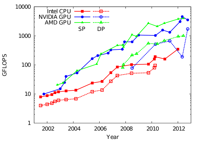
Figure 1: Theoretical peak performance of Intel CPUs and NVIDIA/AMD GPUs, measured in GFLOPS (gigaFLOPS, i.e., billion floating-point operations per second), over the past decade. “SP” and “DP” refer to single and double precision, respectively. Note that the performance is presented in logarithmic scale. Source: John Owens personal communication and vendor specifications.

2.1 Programming GPUs

The current generation of GPU application programming interfaces (APIs), such as CUDA [NVIDIA:2011wf] and OpenCL [Munshi:2011wk], enables a C-like programming experience while exposing the underlying massively parallel architecture. Fortunately, this avoids programming in the graphics pipeline directly. We will focus our discussion on CUDA, a programming platform created and supported by NVIDIA, but OpenCL, an open-source framework supported by multiple vendors, is similar so the same concepts apply (albeit with slightly different names for equivalent features). This section is not intended to function as a complete reference for programming CUDA applications, but only to give a brief overview of the CUDA paradigm. Interested readers should see the textbooks, e.g., by Kirk and Hwu [Kirk:2010we] and Sanders and Kandrot [Sanders:2010tq].

In CUDA, a parallel function is known as a “kernel,” which consists of many threads that perform tasks concurrently. Functions intended for operation on the GPU (the device) and the CPU (the host) are preceded with __device__ and __host__, respectively. Kernel functions are indicated with __global__. Threads are organized into three-dimensional blocks, which in turn are organized into a two-dimensional grid. All threads in a grid execute the same kernel function. The specific location (coordinate) of a thread inside the hierarchy of blocks and grids can be accessed using the variables threadIdx and blockIdx; the dimensions of the block (i.e., the number of threads) and grid (i.e., the number of blocks) can be retrieved using blockDim and gridDim, respectively.

Figure 2 shows a simple kernel function for adding two vectors, compared with an equivalent CPU function. Note that instead of looping through the elements, the threads of the kernel function independently and concurrently add the elements of the two vectors. In general, parallelizing applications for use on GPUs follows this pattern, replacing loops with kernel functions where data may be operated on independently. In this example, both the addend vectors and the sum vector are stored in the GPU’s global memory, which is accessible to all threads in a kernel. Memory on the device must be allocated using the cudaMalloc function prior to the kernel launch, and memory must be explicitly transferred between the host and the device outside the kernel using the cudaMemcpy function. The structures of the thread blocks and grid are specified using the dimBlock and dimGrid variables. In the example given in Fig. 2, for simplicity, both are one-dimensional arrays, with the grid consisting of one block for each element in the vector.

⬇

// C vector addition

void vector_Add (int size, const float *a,

const float *b, float *c) {

for (int i = 0; i < size; ++i) {

c[i] = a[i] + b[i];

}

}

int main (void) {

int size = 10;

...

vector_Add (size, A, B, C);

...

}

⬇

// CUDA vector addition

__global__ void vector_Add_CUDA (int size,

const float *a, const float *b, float *c) {

int ind = blockIdx.x * blockDim.x + threadIdx.x;

c[ind] = a[ind] + b[ind];

}

int main (void) {

int size = 10;

...

dim3 dimGrid (size, 1); dim3 dimBlock (1, 1);

vector_Add_CUDA <<<dimGrid, dimBlock>>>(size, Ad, Bd, Cd);

...

}

Figure 2: Examples of vector addition on the CPU (top) and the GPU (bottom).

Another avenue for accelerating applications using GPUs is OpenACC [OpenACC:2011vn, Reyes:2012wg], which uses compiler directives (e.g., #pragma) placed in Fortran, C, and C++ codes to identify sections of code to be run in parallel on GPUs. This approach is similar to OpenMP [Dagum:1998hb, Chandra:2001ts, Board:2011wl] for parallelizing work across multiple CPUs or CPU cores that share memory. OpenACC is an open standard being jointly developed by NVIDIA, Cray, the Portland Group, and CAPS. Since OpenACC is relatively new and immature, only a few groups have used OpenACC thus far to accelerate their applications. Wienke et al. [Wienke:2012vj] found that OpenACC achieved 80% of the performance of OpenCL in simulations of bevel gear cutting, but only 40% in solving the neuromagnetic inverse problem in the neuroimaging technique magnetoencephalography (reconstructing focal activity in the brain). Reyes et al. [Reyes:2012] showed a similar range of performance, comparing OpenACC with CUDA implementations of LU decomposition, a thermal simulation tool, and a nonlinear global optimization algorithm for DNA sequence alignments. Recently, Levesque et al. [Levesque:2012] reported on their experience hybridizing Sandia National Laboratory’s massively parallel direct numerical simulation code S3D from MPI-only to MPI/OpenMP/OpenACC for three levels of parallelism; we will discuss their results in greater detail in Section LABEL:sec:reactive.

⬇

// OpenACC vector addition

#pragma acc kernels

void vector_Add (int size, const float *restrict a,

const float *restrict b, float *restrict c) {

for (int i = 0; i < size; ++i) {

c[i] = a[i] + b[i];

}

}

int main (void) {

int size = 10;

...

vector_Add (size, A, B, C);

...

}

Figure 3: Example of vector addition using OpenACC directives.

Figure 3 shows the vector addition example with OpenACC compiler directives. With the exception of the restrict keyword added to the function arguments, the only modification to the original CPU version is the single #pragma acc line added before the loop. The main benefit of the OpenACC approach (as well as OpenMP) is that compatible programs may be accelerated without modifying the underlying source code—a non-OpenACC-enabled compiler would treat the directives as comments. Fortran code is handled similarly, albeit with a different directive indicator syntax (C$ACC or !$acc rather than #pragma acc). This contrasts greatly with porting applications written for the CPU to either CUDA or OpenCL, which must be completely rewritten. This convenience comes at the cost of slightly degraded performance, but OpenACC allows researchers to accelerate existing code in a matter of hours, rather than days or weeks. We will compare the performance of OpenACC implementations of our case studies in Section 3.

2.2 GPU performance considerations

In this section we will discuss some topics related to GPU performance, with an emphasis on configuring appropriate device memory and thread execution. For a more comprehensive source, see the textbook by Kirk and Hwu [Kirk:2010we]. As before, we focus on CUDA programming and its naming conventions, while the same principles apply to OpenCL.

Selecting appropriate memory types for different data is the first place to begin improving the performance of a GPU program. Global memory, which the CPU uses to transfer data to and from the GPU, is accessible to all threads in a grid. However, accessing the global memory is fairly slow, and many threads attempting to access the global memory will build up traffic congestion—further slowing communication. In fact, one measure of the performance of a GPU application is the compute to global memory access (CGMA) ratio, which is the ratio of floating point computations to global memory access calls. If the CGMA ratio is around one, then the performance of a GPU application will be limited by the global memory access latency rather than the floating-point processing speed of the particular GPU hardware. A GPU application can only achieve best performance if the CGMA ratio is much higher than one. Typically, excess global memory use is eliminated by using other, faster GPU memory types.

Constant memory offers one alternative to global memory when global access is needed. This is read only, and offers high bandwidth when all threads access the same memory location simultaneously. The CPU transfers data to constant memory on the device before a kernel is executed, and this data cannot be modified by the GPU. Similar to constant memory is texture memory, which is also read-only and available to all threads. Texture memory is cache-optimized for two-dimensional access, as it is a descendent of the GPU’s display capabilities (textures map a two-dimensional image to a three-dimensional surface).

There are also device memory types accessible at the block and thread levels. Shared memory is allocated for each thread block, and is an efficient way for threads in the same block to cooperate—it is roughly 100 times faster than global memory. Registers are private memory blocks available to each thread which also offer fast access. In addition, threads have access to private local memory, which is actually stored in the global memory (and has the corresponding slow access time). Automatic arrays (arrays declared with non-constant size) are stored in the local memory in CUDA, so these should be avoided. Instead, only arrays with a constant size when compiling should be used. Since each GPU offers a limited amount of memory, properly configuring memory is an important task in designing an application. In general, memory will be the limiting factor governing the number of concurrent threads; for example, each thread block offers a limited amount of shared memory and registers.

Another performance consideration relates to the execution of threads. Recall that threads are organized into blocks, which are in turn organized in a grid. Thread blocks can be executed by the GPU in any order, but blocks are not necessarily execution units themselves. Instead, blocks are partitioned into “warps” for execution. In the current generation of CUDA devices, each warp consists of 32 threads. If a block consists of more than 32 threads, the block is partitioned into multiple warps based on the thread index (e.g., threadIdx). A block whose size is not divisible by 32 will be padded with extra threads. All threads in a warp must follow the same instruction path, otherwise threads will diverge and reduce performance significantly. For example, if some threads in warp execute the if statement in an if-then-else construct, while others follow the else path, the GPU can no longer execute the threads concurrently and multiple passes are required (in this example, doubling the execution time). To avoid thread divergence, thread blocks should be organized so that warps follow the same control paths.

It is impossible to avoid using global memory since it is the primary route to transferring data between the CPU and GPU. One way to improve the performance of global memory access is to exploit “memory coalescing” techniques. Understanding coalescing requires some insight into the physical nature of global memory. On CUDA-enabled GPU devices, global memory is typically implemented using dynamic random access memory (DRAM), the same type used on personal computers and workstations. DRAM stores bits of data as tiny electrical charges in small capacitors; reading memory from DRAM cells requires a sensor to share and measure these charges. In order to speed up this relatively slow procedure, the sensor accesses consecutive memory locations around the requested location to increase the data read rate. This hardware behavior can be exploited by instructing threads in the same warp to access consecutive memory locations. If this is detected, the GPU will automatically coalesce (or combine) these memory accesses into a single operation, allowing much higher global memory bandwidth. Interested readers should see Kirk and Hwu [Kirk:2010we] and Jang et al. [Jang:2011ct] for more detail and examples.

Current-generation GPUs have limited bandwidth to process instructions (e.g., floating-point calculations, conditional branches). One common way to improve performance by removing unnecessary instructions is to perform loop unrolling. This avoids both conditional branch instructions (checking if the loop is finished) and the loop counter update. Also, the indices of accessed arrays are now constants rather than changing variables, enabling further optimization. In some compilers, this can be achieved with a #pragma unroll compiler directive preceding the loop, but, where practical, manual unrolling ensures high performance.

Another consideration that is particularly relevant to scientific computations on the GPU is the use of hardware-accelerated transcendental functions, which are significantly faster than corresponding software versions. These can be called by prefixing functions with “__”, e.g., cos() becomes __cos(). Currently, these hardware functions are limited to single-precision calculations; only the software versions of double-precision functions are available, although this may change in the future. The enhanced performance comes at the cost of slightly reduced accuracy. For example, the maximum ulp (“units in the last place”) errors of the software exp(x) and hardware __exp(x) are 2 and $2+\text{floor}\left(\left|1.16x\right|\right)$, respectively. The CUDA Programming Guide describes the error of all the available hardware and software functions [NVIDIA:2011wf]. Automatic use of the hardware functions can also be achieved with the compiler flag “-use_fast_math,” which automatically converts all potential (single-precision) functions to their hardware equivalents.

3 Case studies

We performed two case studies, relevant to CFD, in order to demonstrate the potential acceleration of CFD applications using graphics processors. For both studies, four versions were compared: single-core CPU, six-core CPU using OpenMP, native GPU using CUDA, and GPU-accelerated using OpenACC. The GPU performance experiments were performed using an NVIDIA Tesla c2075 GPU with $6\text{\,}\mathrm{GB}$ of global memory. An Intel Xeon X5650 CPU, running at $2.67\text{\,}\mathrm{GHz}$ with $256\text{\,}\mathrm{kB}$ of L2 cache memory per core and $12\text{\,}\mathrm{MB}$ of L3 cache memory, served as the host processor for the GPU calculations and ran the single-core CPU and OpenMP calculations.

We used the GNU Compiler Collection (gcc) version 4.6.2 (with the compiler options “-O3 -ffast-math -std=c99 -m64”) to compile the CPU programs, the PGI Compiler toolkit version 12.9 to compile the OpenMP (“-fast -mp”) and OpenACC (“-acc -ta=nvidia,cuda4.2,cc20 -lpgacc”) versions, and the CUDA 5.0 compiler nvcc version 0.2.1221 (“-O3 -arch=sm_20 -m64”) to compile the GPU version. The functions cudaSetDevice() and acc_init() were used to hide any device initialization delay in the CUDA and OpenACC implementations, respectively.

3.1 Laplace solver

3.1.1 Methodology

The first case study we performed consisted of solving Laplace’s equation for heat conduction in a square plate. The boundary conditions were a constant zero (nondimensionalized) temperature along the sides and bottom, and a constant temperature of one along the top. Laplace’s equation alone is a fairly trivial example, but due to its relevance to many approaches to solving the pressure term in the Navier–Stokes equations we included it here. Using the finite volume method with a constant grid, the discretization of the equation is:

$$\nabla^{2}T =\frac{\partial^{2}T}{\partial x^{2}}+\frac{\partial^{2}T}{\partial y^{2}}=0$$ (1)

$$a_{P}T_{P} =a_{W}T_{W}+a_{E}T_{E}+a_{S}T_{S}+a_{N}T_{N}+S_{u}$$ (2)

$$a_{P} =a_{W}+a_{E}+a_{S}+a_{N}-S_{P}$$ (3)

$$a_{W} =a_{E}=k\frac{\delta y}{\delta x}$$ (4)

$$a_{S} =a_{N}=k\frac{\delta x}{\delta y}$$ (5)

where k is the thermal conductivity, $\delta x$ and $\delta y$ are the grid spacing in the $x$ and $y$ directions respectively, and $S_{u}$ and $S_{P}$ represent source terms used for boundary conditions. All quantities are dimensionless. For the given boundary conditions,

$$x =0:\quad a_{W}=0$$ (6)

$$x =1:\quad a_{E}=0$$ (7)

$$y =0:\quad a_{S}=0$$ (8)

$$y =1:\quad\begin{cases}a_{N}=0\\ S_{u}=2kw\frac{\delta x}{\delta y}\\ S_{P}=-2kw\frac{\delta x}{\delta y}\end{cases}$$ (9)

where $w$ is the thickness of the plate.

We solved Eq. (2) iteratively using the red-black Gauss–Seidel (GS) method with successive over-relaxation (SOR). Traditional GS or SOR approaches are not suitable for use on parallel CPU or GPU systems since the order of operations is neither known nor controllable, and conflicts in accessing and writing to memory may occur (although Jacobi iteration is suitable for parallel/GPU implementation, since calculation of new values depends only on old values). Red-black SOR solves this problem by coloring the grid like a checkerboard, alternating red and black cells. First, the algorithm updates values at red cells—which depend only on black cells—then black cells—which depend only on red cells. Both of these operations can be performed in parallel. Red-black SOR was first used to solve a system of linear equations on vector and parallel computer systems by Adams and Ortega [Adams:1982], although introduced earlier (e.g., by Young [Young:1971]). Liu et al. [Liu:2011] provided a more detailed analysis of red-black SOR implemented on GPUs.

In order to show the importance of redesigning algorithms for GPUs, we enabled flags in the code for various optimization steps. The initial, naively implemented GPU code matched the original serial CPU version: two GPU kernel functions updated the temperatures in the red and black cells, returning residual values for every cell each iteration (in order to determine when the SOR algorithm stops). In a first optimization step, we organized the thread blocks such that threads in the same warp access adjacent locations in global memory to activate coalescing. Next, we improved this coalesced memory access by storing the temperature values for the red and black cells in two arrays—such that read and write operations always accessed neighboring memory locations, rather than every other. Finally, to minimize the GPU-CPU memory transfer each iteration, we used shared memory to calculate the maximum residual of each block, such that only a single value per block needed to be transferred back to the CPU rather than values for all threads. Additionally, in order to avoid thread divergence caused by conditional statements for boundary conditions, “ghost cells” that held constant temperatures of zero surrounded the computational domain. Therefore, at the boundaries these cells could be accessed instead of needing a conditional statement to avoid an out-of-bounds array access error.

We also explored using texture memory to store the constant coefficient arrays (e.g., $a_{P}$, $a_{W}$, etc.), but found the performance to be equivalent or worse than coalesced global memory. In addition, for single-precision calculations “atomic” memory operations can be used to allow threads in different blocks to access the same points in global memory. This enables global reduction operations, in this case allowing a single residual value to be transferred from the GPU to the CPU per iteration rather than one per block as with the shared memory alone. We found that using atomic operations improved performance about 5% or less; the savings in memory transfer likely balanced the generally low performance of such operations.

The OpenACC solver was based on the CPU solver, with directives instructing the compiler to use the GPU on loops matching the kernel functions of the GPU solver—no other changes to the underlying CPU code were made. The OpenMP solver was created the same way, using the appropriate compiler directives. No specific optimization instructions were given to either the OpenMP or OpenACC solver; rather, we allowed the compiler to manage this automatically.

In order to study the performance of the native GPU and OpenACC solvers against the CPU versions, we varied the mesh size from 128² to 8192². The source code was written in standard and CUDA C for the CPU and GPU versions, respectively, with compiler directives added to the CPU version to create OpenMP and OpenACC versions. In the fully optimized (corresponding to the shared-memory implementation) CUDA-based GPU version, we kept a constant block size of 128 $\times$ 1 (except for the case of the mesh size being 128, where we used 64 $\times$ 1), aligned with either the vertical or horizontal directions depending on if the global memory coalescing flag was enabled (arranged so that thread warps aligned with adjacent locations in memory, as described above). The naive, coalesced global memory, and improved coalescing configurations used grid sizes of $N\times\nicefrac{{N}}{{B}}$, $\nicefrac{{N}}{{B}}\times N$, and $\nicefrac{{N}}{{2B}}\times N$, respectively, where N is the number of mesh cells in one direction (e.g., 512) and B is the block size (e.g., 128). The fully-optimized, shared memory configuration built on the improved coalescing configuration and thus used the same grid size. In order to perform a fair comparison, the serial CPU code—and, therefore, the OpenMP and OpenACC versions—used the red-black SOR algorithm, with separate arrays for the red and black pressure values in the same manner as the optimized GPU versions.

3.1.2 Results

First, we demonstrate the importance of redesigning algorithms for GPU computing, taking into consideration GPU-specific performance improvements. Figure 4 shows the performance of the naive GPU solver and with various optimization steps for double-precision calculations. Single-precision results showed similar trends, requiring about half the computational time. By specifically optimizing the code for execution on graphics cards, we increased the performance of the GPU code by up to a factor of nearly 19 compared to the naive implementation.

Next, we compared the performance of the single-core CPU, six-core CPU, fully optimized CUDA-based GPU, and OpenACC-based GPU solvers over a wide range of mesh sizes for double-precision calculations, shown in Fig. 5. At mesh sizes of 1024² and above, the GPU solver ran faster than the CPU solver on either one or six cores; at most, the GPU solver performed up to about 10 and 4.6 times faster than the single-core and six-core CPU solvers, respectively, for double precision. The single-precision code performed similarly: the CUDA-based GPU solver ran about 16 and 4.6 faster than the single- and six-core CPU versions, at best.

At smaller mesh sizes, the OpenACC implementation ran nearly five times slower than the native, fully optimized GPU version, but as the mesh size increased this gap decreased to nearly zero, demonstrating almost equal performance at the largest grid sizes. This behavior was replicated in single-precision calculations, although the OpenACC solver performed about 8% slower at the largest grid sizes and 6.9 times slower at the smallest mesh sizes.

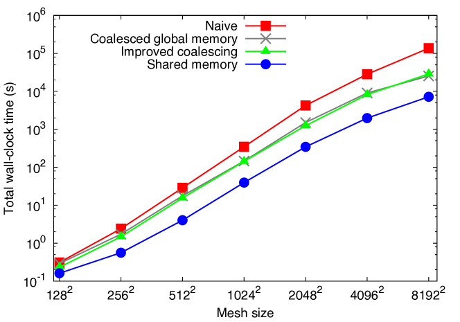
Figure 4: Performance of GPU solver with various optimization approaches, for a wide range of mesh sizes. The “shared memory” implementation is fully optimized.

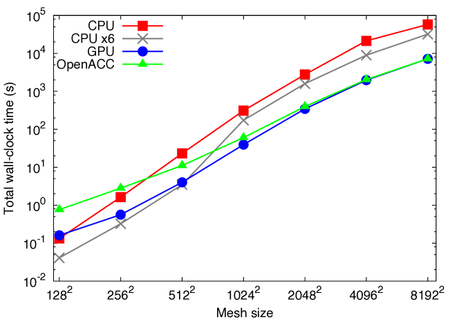
Figure 5: Performance comparison of the CPU Laplace solver on one core and six cores (via OpenMP), the fully optimized CUDA-based GPU solver, and OpenACC-based GPU solver, for a wide range of mesh sizes.

Note that we did not optimize the block size for the GPU solver, but left it constant for this simple demonstration. Similarly, we allowed the OpenACC compiler to determine the optimal configuration, rather than manually adjust its equivalents (“gang” and “vector” sizes). More in-depth optimization could further improve performance for both implementations.

Finally, we observed that while the native fully optimized GPU solver showed the best performance for larger grid sizes, the OpenACC version performed nearly as well, especially for double-precision calculations. These results suggest that OpenACC is a good alternative to writing native GPU code, especially considering the fact that porting CPU applications to CUDA can require days to weeks of work while adding the OpenACC compiler directives takes only hours or even minutes. However, OpenACC support is currently limited, and can only be applied to applications that already favor parallelization—such as those based on loops with independent iterations—and where functions may be inlined. With this in mind, OpenACC is a good choice to quickly accelerate existing code and determine potential speedup, while writing native GPU applications offers the highest potential performance if fully optimized. In either case, algorithms may need to be redesigned in order to support massive parallelization, although this was not necessary in the current example.

3.2 Lid-driven cavity flow

3.2.1 Methodology

The second case study consisted of solving the two-dimensional, laminar incompressible Navier–Stokes equations based on the finite difference method, using the solution procedure given by Griebel et al. [Griebel:1998]. The domain was discretized with a uniform, staggered grid (i.e., the pressure values are located at the centers of grid cells while velocity values are located along the edges). Briefly, the discretized momentum (assuming no gravity/body-force terms) and pressure-Poisson equations are: rCl F_i,j^(n) & = u_i,j^(n)
+  δt ( 1Re ( [ ∂2u ∂x2 ]_i,j^(n) + [ ∂2u ∂y2 ]_i,j^(n) ) - [ ∂(u2) ∂x ]_i,j^(n) - [ ∂(uv) ∂y ]_i,j^(n) ) ,
3ri = 1, …, i_max - 1,  j = 1, …, j_max ,
G_i,j^(n) = v_i,j^(n)
+  δt ( 1Re ( [ ∂2v ∂x2 ]_i,j^(n) + [ ∂2v ∂y2 ]_i,j^(n) ) - [ ∂(uv) ∂x ]_i,j^(n) - [ ∂(v2) ∂y ]_i,j^(n) ) ,
3ri = 1, …, i_max,  j = 1, …, j_max - 1 , rCl pi+1,j(n+1)- 2 pi,j(n+1)+ pi-1,j(n+1)(δx)2 & + pi,j+1(n+1)- 2 pi,j(n+1)+ pi,j-1(n+1)(δy)2
= 1δt ( Fi,j(n)- Fi-1,j(n)δx + Gi,j(n)- Gi,j-1(n)δy )
3ri = 1, …, i_max,  j = 1, …, j_max ,
3Cu_i,j^(n+1) = F_i,j^(n+1) - δtδx ( p_i+1,j^(n+1) - p_i,j^(n+1) ) ,
3r i = 1, …, i_max - 1,  j = 1, …, j_max,
3Cv_i,j^(n+1) = G_i,j^(n+1) -