Infrared Spectroscopic Survey of the Quiescent Medium of Nearby Clouds: I. Ice Formation and Grain Growth in Lupus

Abstract

Infrared photometry and spectroscopy (1-25 ${\rm\mu m}$) of background stars reddened by the Lupus molecular cloud complex are used to determine the properties of the grains and the composition of the ices before they are incorporated into circumstellar envelopes and disks. H₂O ices form at extinctions of $A_{\rm K}=0.25\pm 0.07$ mag ($A_{\rm V}=2.1\pm 0.6$). Such a low ice formation threshold is consistent with the absence of nearby hot stars. Overall, the Lupus clouds are in an early chemical phase. The abundance of H₂O ice (2.3$\pm 0.1\times 10^{-5}$ relative to $N_{\rm H}$) is typical for quiescent regions, but lower by a factor of 3-4 compared to dense envelopes of YSOs. The low solid CH₃OH abundance ($<3-8$% relative to H₂O) indicates a low gas phase H/CO ratio, which is consistent with the observed incomplete CO freeze out. Furthermore it is found that the grains in Lupus experienced growth by coagulation. The mid-infrared ($>5$ ${\rm\mu m}$) continuum extinction relative to $A_{\rm K}$ increases as a function of $A_{\rm K}$. Most Lupus lines of sight are well fitted with empirically derived extinction curves corresponding to $R_{\rm V}\sim 3.5$ ($A_{\rm K}=0.71$) and $R_{\rm V}\sim 5.0$ ($A_{\rm K}=1.47$). For lines of sight with $A_{\rm K}>1.0$ mag, the $\tau_{9.7}/A_{\rm K}$ ratio is a factor of 2 lower compared to the diffuse medium. Below 1.0 mag, values scatter between the dense and diffuse medium ratios. The absence of a gradual transition between diffuse and dense medium-type dust indicates that local conditions matter in the process that sets the $\tau_{9.7}/A_{\rm K}$ ratio. This process is likely related to grain growth by coagulation, as traced by the $A_{7.4}/A_{\rm K}$ continuum extinction ratio, but not to ice mantle formation. Conversely, grains acquire ice mantles before the process of coagulation starts.

1. Introduction

Dense cores and clouds are the birthplaces of stars and their planetary systems (e.g., Evans et al. 2009), and it is therefore important to know their composition. Gas phase abundances are strongly reduced in these environments as species freeze out onto grains (CO, CS; Bergin et al. 2001), and new molecules are formed by grain surface chemistry (e.g., H₂O, CH₄, CO₂, Tielens & Hagen 1982). Infrared spectroscopy of the vibrational absorption bands of ices against the continuum emission of background stars is thus a powerful tool to determine the composition of dense media (Whittet et al., 1983).

The Taurus Molecular Cloud (TMC) is the first cloud in which frozen H₂O (Whittet et al., 1983), CO (Whittet et al., 1985), and CO₂ (Whittet et al., 1998) were detected using background stars. This is also the case for the 6.85 ${\rm\mu m}$ band (Knez et al., 2005), whose carrier is uncertain (possibly NH${}_{4}^{+}$). Recently solid CH₃OH was discovered toward several isolated dense cores (Boogert et al., 2011; Chiar et al., 2011). These and follow up studies showed that the ice abundances depend strongly on the environment. The extinction threshold for H₂O ice formation is a factor of two higher for the Ophiuchus (Oph) cloud than it is for TMC ($A_{\rm V}=$10-15 versus 3.2 mag; Tanaka et al. 1990; Whittet et al. 2001). These variations may reflect higher local interstellar radiation fields (e.g., hot stars in the Oph neighborhood), which remove H₂O and its precursors from the grains either by photodesorption or sublimation at the cloud edge (Hollenbach et al., 2009). Deeper in the cloud, ice mantle formation may be suppressed by shocks and radiation fields from Young Stellar Objects (YSOs), depending on the star formation rate (SFR) and initial mass function (IMF). The latter may apply in particular to the freeze out of the volatile CO species, and, indirectly, to CH₃OH. CO freeze out sets the gas phase H/CO ratio, which sets the CH₃OH formation rate (Cuppen et al., 2009). High CH₃OH abundances may be produced on time scales that depend on dust temperature and other local conditions (e.g., shocks). This may well explain the observed large CH₃OH abundance variations: $N$(CH₃OH)/$N$(H₂O)$\leq 3$% toward TMC background stars (Chiar et al., 1995) and $\sim 10$% toward some isolated dense cores (Boogert et al., 2011).

The number of dense clouds and the number of sight-lines within each cloud observed with mid-infrared spectroscopy ($\lambda>5$ ${\rm\mu m}$) is small. Ice and silicate inventories were determined toward four TMC and one Serpens cloud background stars (Knez et al., 2005). Many more lines of sight were recently studied toward isolated dense cores (Boogert et al., 2011). These cores have different physical histories and conditions, however, and may not be representative of dense clouds. Their interstellar media lack the environmental influences of outflows and the resulting turbulence often thought to dominate in regions of clustered star formation (clouds). Their star formation time scales can be significantly larger due to the dominance of magnetic fields over turbulence and the resulting slow process of ambipolar diffusion (Shu et al., 1987; Evans, 1999). Over time, the ice composition likely reflects the physical history of the environment. This, in turn may be preserved in the ices in envelopes, disks and planetary systems. Quiescent cloud and core ices are converted to more complex organics in YSO envelopes (Öberg et al., 2011). 2D collapse models of YSOs show that subsequently all but the most volatile envelope ices (CO, N₂) survive the infall phase up to radii $>10$ AU from the star (Visser et al., 2009). They are processed at radii $<30$ AU, further increasing the chemical complexity. For this reason, it is required to determine the ice abundances in a larger diversity of quiescent environments. A Spitzer spectroscopy program (P.I. C. Knez) was initiated to observe large samples of background stars, selected from 2MASS and Spitzer photometric surveys of the nearby Lupus, Serpens, and Perseus Molecular Clouds. This paper focuses on the Lupus cloud. Upcoming papers will present mid-infrared spectroscopy of stars behind the Serpens and Perseus clouds.

The Lupus cloud complex is one of the main nearby low mass star forming regions. It is located near the Scorpius-Centaurus OB association and consists of a loosely connected group of clouds extended over $\sim$20 degrees (e.g., Comerón 2008). The Lupus I, III, and IV clouds were mapped with Spitzer/IRAC and MIPS broad band filters, and analyzed together with 2MASS near infrared maps (Evans et al., 2009). In this paper, only stars behind the Lupus I and IV clouds will be studied. This is the first study of Lupus background stars. Compared to other nearby clouds, the Lupus clouds likely experienced less impact from nearby massive stars and internal YSOs. While OB stars in the Scorpius-Centaurus association may have influenced the formation of the clouds, they are relatively far away ($\sim 17$ pc) and their current impact on the Lupus clouds is most likely smaller compared to that of massive stars on the Oph, Serpens, and Perseus clouds (Evans et al., 2009). Likewise, star formation within the Lupus clouds is characterized by a relatively low SFR, 0.83 M_⊙/Myr/pc², versus 1.3, 2.3, and 3.2 for Perseus, Ophiuchus and the Serpens clouds, respectively (Evans et al., 2009). In addition, the mean stellar mass of the YSOs (0.2 M_⊙; Merín et al. 2008) is low compared to that of other clouds (e.g., Serpens 0.7 M_⊙) as well as to that of the IMF (0.5 M_⊙). Lupus also stands out with a low fraction of Class I YSOs (Evans et al., 2009). Within Lupus, the different clouds have distinct characteristics. While Herschel detections of prestellar cores and Class 0 YSOs indicate that both Lupus I and IV have an increasing SFR, star formation in Lupus IV has just begun, considering its low number of prestellar sources (Rygl et al., 2013). The Lupus IV cloud is remarkable in that the Spitzer-detected YSOs are distributed away from the highest extinction regions. Extinction maps produced by the c2d team show that Lupus IV contains a distinct extinction peak, while Lupus I has a lower, more patchy extinction ($A_{\rm V}$=32.6 versus 26.5 mag at a resolution of 120^′′). It is comparable to the Serpens cloud (33.5 mag at 120^′′ resolution), but factors of 1.5-2 lower compared to the Perseus and Ophiuchus clouds.

Both volatiles and refractory dust can be traced in the mid-infrared spectra of background stars. This paper combines the study of ice and silicate features with line of sight extinctions. The ice formation threshold toward Lupus is investigated as well as the relation of the 9.7 ${\rm\mu m}$ band of silicates with the continuum extinction. The 9.7 ${\rm\mu m}$ band was extensively studied toward background stars tracing dense clouds and cores. While no differences were found between clouds and cores, its strength and shape are distinctly different compared to the diffuse ISM. The peak optical depth of the 9.7 ${\rm\mu m}$ band relative to the K-band continuum extinction is a factor of $\sim$2 smaller in dense lines of sight (Chiar et al., 2007; Boogert et al., 2011; Chiar et al., 2011). The short wavelength wing is also more pronounced. Grain growth cannot explain these effects simultaneously (van Breemen et al., 2011). On the other hand, the same spectra of background stars show grain growth by increased continuum extinction at longer wavelengths (up to at least 25 ${\rm\mu m}$; McClure 2009; Boogert et al. 2011), in agreement with broad band studies (Chapman et al., 2009).

The selection of the background stars is described in §2, and the reduction of the ground-based and Spitzer spectra in §3. In §4.1, the procedure to fit the stellar continua is presented, a crucial step in which ice and silicate features are separated from stellar features and continuum extinction. Subsequently, in §4.2, the peak and integrated optical depths of the ice and dust features are derived, as well as column densities for the identified species. Then in §4.3, the derived parameters $A_{\rm K}$, $\tau_{3.0}$, and $\tau_{9.7}$ are correlated with each other. §5.1 discusses the Lupus ice formation threshold and how it compares to other clouds. The slope of the $A_{\rm K}$ versus $\tau_{3.0}$ relations is discussed in §5.2. The ice abundances are put into context in §5.3. The $A_{\rm K}$ versus $\tau_{9.7}$ relation, and in particular the transition from diffuse to dense cloud values, is discussed in §5.4. Finally, the conclusions are summarized and an outlook to future studies is presented in §6.

Table 1Source Sample 

Source	Cloud	AOR key	Module	$\lambda_{\rm NIR}$
2MASS J				${\rm\mu m}$
15382645$-$3436248	Lup I	23077120	SL, LL2	1.88-4.17
15423699$-$3407362	Lup I	23078400	SL, LL2	1.88-4.17
15424030$-$3413428d	Lup I	23077888	SL, LL2	1.88-4.17
15425292$-$3413521	Lup I	23077632	SL, LL2	1.88-5.06
15444127$-$3409596	Lup I	23077376	SL, LL	1.88-4.17
15450300$-$3413097	Lup I	23077376	SL, LL	1.88-5.06
15452747$-$3425184	Lup I	23077888	SL, LL2	1.88-5.06
15595783$-$4152396	Lup IV	23079168	SL, LL2	1.88-4.17
16000067$-$4204101	Lup IV	23079680	SL, LL2	1.88-4.17
16000874$-$4207089	Lup IV	23078912	SL, LL	1.88-4.17
16003535$-$4209337	Lup IV	23081216	SL, LL2	1.88-4.17
16004226$-$4146411	Lup IV	23079424	SL, LL2	1.88-4.17
16004739$-$4203573	Lup IV	23082240	SL, LL2	1.88-4.17
16004925$-$4150320	Lup IV	23079936	SL, LL	1.88-5.06
16005422$-$4148228	Lup IV	23079936	SL, LL	1.88-4.17
16005511$-$4132396	Lup IV	23078656	SL, LL	1.88-4.17
16005559$-$4159592	Lup IV	23079680	SL, LL2	1.88-4.17
16010642$-$4202023	Lup IV	23081984	SL, LL2	1.88-4.17
16011478$-$4210272	Lup IV	23079168	SL, LL2	1.88-4.17
16012635$-$4150422	Lup IV	23081728	SL, LL2	1.88-4.17
16012825$-$4153521	Lup IV	23081472	SL, LL2	1.88-4.17
16013856$-$4133438	Lup IV	23079424	SL, LL2	1.88-4.17
16014254$-$4153064	Lup IV	23082496	SL, LL2	1.88-5.06
16014426$-$4159364	Lup IV	23080192	SL, LL2	1.88-4.17
16015887$-$4141159	Lup IV	23078656	SL, LL	1.88-4.17
16021102$-$4158468	Lup IV	23080192	SL, LL2	1.88-5.06
16021578$-$4203470	Lup IV	23078656	SL, LL	1.88-4.17
16022128$-$4158478	Lup IV	23080704	SL, LL2	1.88-4.17
16022921$-$4146032	Lup IV	23078912	SL, LL	1.88-4.17
16023370$-$4139027	Lup IV	23080960	SL, LL2	1.88-4.17
16023789$-$4138392	Lup IV	23080448	SL, LL2	1.88-4.17
16024089$-$4203295	Lup IV	23080448	SL, LL2	1.88-4.17

2. Source Selection

Background stars were selected from the Lupus I and IV clouds that were mapped with Spitzer/IRAC and MIPS by the c2d Legacy team (Evans et al., 2003, 2007). The maps are complete down to $A_{\rm V}$=3 and $A_{\rm V}$=2 for Lupus I and IV, respectively (Evans et al., 2003). The selected sources have an overall SED (2MASS 1-2 ${\rm\mu m}$, IRAC 3-8 ${\rm\mu m}$, MIPS 24 ${\rm\mu m}$) of a reddened Rayleigh-Jeans curve. They fall in the “star” category in the c2d catalogs and have MIPS 24 ${\rm\mu m}$ to IRAC 8 ${\rm\mu m}$ flux ratios greater than 4. In addition, fluxes are high enough ($>$10 mJy at 8.0 ${\rm\mu m}$) to obtain Spitzer/IRS spectra of high quality (S/N$>$50) within $\sim$20 minutes of observing time per module. This is needed to detect the often weak ice absorption features and determine their shapes and peak positions. This resulted in roughly 100 stars behind Lupus I and IV. The list was reduced by selecting $\sim$10 sources in each interval of $A_{\rm V}$: 2-5, 5-10, and $>$10 mag (taking $A_{\rm V}$ from the c2d catalogs) and making sure that the physical extent of the cloud is covered. The final list contains nearly all high $A_{\rm V}$ lines of sight. At low extinctions, many more sources were available and the brightest were selected. The observed sample of 25 targets toward Lupus IV, and 7 toward Lupus I is listed in Table 1. The analysis showed that the SEDs of three Lupus I and two Lupus IV sources cannot be fitted with stellar models (§4.1). One of these is a confirmed Class III “cold disk” YSO (2MASS J$15424030-3413428$; Merín et al. 2008). The ice and dust feature strengths and abundances are derived for these five sources, but they are not used in the quiescent medium analysis.

Figure 1 plots the location of the observed background stars on extinction maps derived from 2MASS and Spitzer photometry (Evans et al., 2007). The maps also show all YSOs identified in the Spitzer study of Merín et al. (2008). Some lines of sight are in the same area as Class I and Flat spectrum sources, but not closer than a few arcminutes.

Figure 1.— Background stars (black filled circles) observed toward the Lupus I (left panel) and Lupus IV (right) clouds, over-plotted on extinction maps (Evans et al., 2007) with contours $A_{K}$=0.25,0.5,1.0,1.5,2.0,2.5,3.0 mag (assuming $A_{\rm V}/A_{\rm K}=7.6$ for $R_{\rm V}=5.0$; Cardelli et al. 1989). The red filled circles indicate Class I YSOs, green filled circles Flat spectrum YSOs, purple filled circles Class II YSOs, and purple open circles Class III YSOs (all from Merín et al. 2008).

3. Observations and Data Reduction

Spitzer/IRS spectra of background stars toward the Lupus I and IV clouds were obtained as part of a dedicated Open Time program (PID 40580). Table 1 lists all sources with their AOR keys, and the IRS modules they were observed in. The SL module, covering the 5-14 ${\rm\mu m}$ range, includes several ice absorption bands as well as the 9.7 ${\rm\mu m}$ band of silicates, and had to highest signal-to-noise goal ($>$50). The LL2 module (14-21 ${\rm\mu m}$) was included to trace the 15 ${\rm\mu m}$ band of solid CO₂ and for a better overall continuum determination, although at a lower signal-to-noise ratio of $>30$. At longer wavelengths, the background stars are weaker, and the LL1 module ($\sim$20-35 ${\rm\mu m}$) was used for only $\sim 30$% of the sources. The spectra were extracted and calibrated from the two-dimensional Basic Calibrated Data produced by the standard Spitzer pipeline (version S16.1.0), using the same method and routines discussed in Boogert et al. (2011). Uncertainties (1$\sigma$) for each spectral point were calculated using the “func” frames provided by the Spitzer pipeline.

The Spitzer spectra were complemented by ground-based VLT/ISAAC (Moorwood et al., 1998) K and L-band spectra. Six bright sources were also observed in the M-band. The observations were done in ESO programs 083.C-0942(A) (visitor mode) and 085.C-0620(A) (service mode) spread over the time frame of 25 June 2009 until 14 August 2010. The K-band spectra were observed in the SWS1-LR mode with a slit width of 0.3”, yielding a resolving power of $R=$1500. Most L- and M-band spectra were observed in the LWS3-LR mode with a slit width of 0.6”, yielding resolving powers of $R=$600 and 800, respectively. The ISAAC pipeline products from the ESO archive could not be used for scientific analysis because of errors in the wavelength scale (the lamp lines were observed many hours from the sky targets). Instead, the data were reduced from the raw frames in a way standard for ground-based long-slit spectra with the same IDL routines used for Keck/NIRSPEC data previously (Boogert et al., 2008). Sky emission lines were used for the wavelength calibration and bright, nearby main sequence stars were used as telluric and photometric standards. The final spectra have higher signal-to-noise ratios than the final ESO/ISAAC pipeline spectra because the wavelength scale of the telluric standards were matched to the science targets before division, using sky emission lines as a reference.

In the end, all spectra were multiplied along the flux scale in order to match broad-band photometry from the 2MASS (Skrutskie et al., 2006), Spitzer c2d (Evans et al., 2007), and WISE (Wright et al., 2010) surveys using the appropriate filter profiles. The same photometry is used in the continuum determination discussed in §4.1. Catalog flags were taken into account, such that the photometry of sources listed as being confused within a 2″ radius or being located within 2″ of a mosaic edge were treated as upper limits. The c2d catalogs do not include flags for saturation. Therefore, photometry exceeding the IRAC saturation limits (at the appropriate integration times) were flagged as lower limits. In those cases, the nearby WISE photometric points were used instead. Finally, as the relative photometric calibration is important for this work, the uncertainties in the Spitzer c2d and 2MASS photometry were increased with the zero-point magnitude uncertainties listed in Table 21 of Evans et al. (2007) and further discussed in their §3.5.3.

4. Results

The observed spectra (left panels of Fig. 2) show the distinct 3.0 and 9.7 ${\rm\mu m}$ absorption features of H₂O ice and silicates on top of reddened stellar continua. These are the first detections of ices and silicates in the quiescent medium of the Lupus clouds. The weaker 6.0, 6.85, and 15 ${\rm\mu m}$ ice bands are evident after a global continuum is subtracted from the spectra (right panels of Fig. 2). Features from the stellar photosphere are present as well (e.g., 2.4 and 8.0 ${\rm\mu m}$). The separation of interstellar and photospheric features is essential for this work and is discussed next.

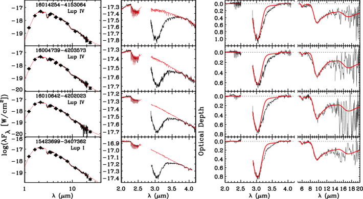
Figure 2.— Left panels: Observed ground-based and Spitzer/IRS spectra combined with broad band photometry (filled circles), and lower limits (open triangles) and 3$\sigma$ upper limits (open circles) thereof. The red lines represent the fitted models, using synthetic stellar spectra (§4.1). The sources are sorted in decreasing ${\rm A_{K}}$ values from top to bottom. Sources labeled with ’X’ have poor long wavelength fits and will not be further treated as background stars. Middle panels: Observed ground-based $K$ and $L$-band spectra. The red lines represent the fitted models (excluding H₂O ice), using stellar spectra from the IRTF database (Rayner et al., 2009). Right panels: Optical depth spectra, derived using the continuum models of the left panels. The red lines indicate the modeled H₂O ice and silicates spectra. For clarity, error bars of the spectral data points are not shown.

Figure 2.— (Continuation)

Figure 2.— (Continuation)

Figure 2.— (Continuation)

4.1. Continuum Determination

The continua for the interstellar ice and dust absorption features were determined in two steps. First, all available photometry and spectra in the 1-4.2 ${\rm\mu m}$ wavelength range were fitted with the full IRTF database of observed stellar spectra (Rayner et al., 2009), reddened using the continuum extinction curves and H₂O ice model further described below. These fits yield accurate values for the peak optical depth of the 3.0 ${\rm\mu m}$ band of H₂O ice ($\tau_{3.0}$), as the continuum shape and photosperic absorption are corrected for simultaneously. Subsequently, the ground-based, WISE, and Spitzer spectral and broad-band photometry over the full 1-30 ${\rm\mu m}$ wavelength range were fitted with thirteen model spectra of giants with spectral types in the range G8 to M9 (Decin et al., 2004; Boogert et al., 2011). These fits yield the peak optical depth of the 9.7 ${\rm\mu m}$ band of silicates, while $\tau_{3.0}$ is fixed to the value found in the IRTF fits. Both fits yield values for the extinction in the $K-$band ($A_{\rm K}$). Both the IRTF and synthetic model fits use the same $\chi^{2}$ minimization routine described in detail in Boogert et al. (2011), and have the same ingredients:

• Feature-free, high resolution extinction curves. Since it is the goal of this work to analyze the ice and dust absorption features, the IRTF database and synthetic stellar spectra must be reddened with a feature-free extinction curve. Such curve can be derived empirically, from the observed spectra themselves. The curve used in Boogert et al. (2011) is derived for a high extinction line of sight ($A_{\rm K}=$3.10 mag) through the isolated core L1014. This curve does not always fit the lower extinction lines of sight through the Lupus clouds. Therefore, empirical, feature-free extinction curves are also derived from two Lupus IV sight-lines: 2MASS J16012635-4150422 ($A_{\rm K}=$1.47) and 2MASS J16015887-4141159 ($A_{\rm K}=$0.71). Throughout this paper, these will be referred to as extinction curves 1 ($A_{\rm K}=$0.71), 2 ($A_{\rm K}=$1.47), and 3 ($A_{\rm K}=$3.10). The three curves are compared in Fig. 3. Clearly, lines of sight with lower $A_{\rm K}$ values have lower mid-infrared continuum extinction. To compare the empirical curves with the models of Weingartner & Draine (2001), the median extinction in the 7.2-7.6 ${\rm\mu m}$ range, relatively free of ice and dust absorption features, is calculated: $A_{7.4}/A_{\rm K}$=0.22, 0.32, and 0.44, for curves 1-3 respectively. Curve 1 falls between the $R_{\rm V}=3.1$ ($A_{7.4}/A_{\rm K}$=0.14) and 4.0 ($A_{7.4}/A_{\rm K}$=0.29) models, and thus corresponds to $R_{\rm V}\sim 3.5$. Curve 2 corresponds to $R_{\rm V}\sim 5.0$, and curve 3 must have $R_{\rm V}$ well above 5.5 ($A_{7.4}/A_{\rm K}$=0.34). To further illustrate this point, $A_{7.4}/A_{\rm K}$ is derived for all lines of sight and over-plotted on the extinction map of Lupus IV in Fig. 4. All lines of sight with $A_{\rm 7.4}$/$A_{\rm K}/>0.30$ lie near the high extinction peaks, while others lie in the low extinction outer regions.

• Laboratory H₂O ice spectra. The optical constants of amorphous solid H₂O at $T=10$ K (Hudgins et al., 1993) were used to calculate the absorption spectrum of ice spheres (Bohren & Huffman, 1983). Spheres with radii of 0.4 ${\rm\mu m}$ fit the typical short wavelength profile and peak position of the observed 3 ${\rm\mu m}$ bands best. While this may not be representative for actual dense cloud grain sizes and shapes, it suffices for fitting the H₂O band profiles and depths.

• Synthetic silicate spectra. As for other dense cloud sight-lines and YSOs, the 9.7 ${\rm\mu m}$ silicate spectra in the Lupus clouds are wider than those in the diffuse ISM (van Breemen et al., 2011; Boogert et al., 2011). No evidence is found for narrower, diffuse medium type silicate bands. Thus, the same synthetic silicate spectrum is used as in Boogert et al. (2011), i.e., for grains small compared to the wavelength, having a pyroxene to olivine optical depth ratio of 0.62 at the 9.7 ${\rm\mu m}$ peak.

Figure 3.— Empirically derived, feature-free extinction curves used in the continuum fitting. The source of each curve is indicated in the plot. The curve for 2MASS J21240517 was derived in Boogert et al. (2011). The curve from Indebetouw et al. (2005) is shown for comparison. It was derived from broad-band photometry and includes absorption by ice and dust features. The triangle, square, and circle represent the extinction at 7.4 ${\rm\mu m}$ for $R_{\rm V}$=3.1, 4.0, and 5.5 models (Weingartner & Draine, 2001), respectively.

Figure 4.— Background stars with a continuum extinction ratio $A_{7.4}/A_{\rm K}>0.30$ (triangles) and $<0.30$ (bullets) plotted on top of the Lupus IV extinction map (same contours as in Fig. 1; Evans et al. 2007).

The results of the continuum fitting are listed in Table 2, and the fits are plotted in Fig. 2 (red lines). Two reduced $\chi^{2}$ values are given: one tracing the fit quality in the 1-4.2 ${\rm\mu m}$ region using the IRTF database, and one tracing the longer wavelengths using the synthetic stellar spectra. The IRTF fits were done at a resolving power of $R=500$ and the reduced $\chi^{2}$ values are very sensitive to the fit quality of the photospheric CO overtone lines at 2.25-2.60 ${\rm\mu m}$, as well as other photospheric lines, including the onset of the SiO $\Delta v=2$ overtone band at 4.0 ${\rm\mu m}$. The wavelength region of 3.09-3.7 ${\rm\mu m}$ is excluded in the $\chi^{2}$ determination because the long wavelength wing of the H₂O ice band is not part of the model. In some cases, the flux scale of the $L-$band spectrum relative to the $K-$band had to be multiplied with a scaling factor to obtain the most optimal fit. These adjustments are attributed to the statistical uncertainties in the broad-band photometry used to scale the observed spectra, i.e., they are generally within 1$\sigma$ of the photometric error bars and at most 2.1$\sigma$ in four cases. Finally, the fits were inspected and $\tau_{3.0}$ values were converted to 3$\sigma$ upper limits in case no distinct 3.0 ${\rm\mu m}$ ice band was present, but rather a shallow, broader residual (dashed lines in Fig. 2).

Table 2Continuum Fit Parameters 

Source	Spectral Type		$A_{\rm K}$	$\tau_{3.0}$	$\tau_{\rm 9.7}$	Ext. Curve	$\chi_{\nu}^{2}$
2MASS J	Model	IRTF	mag				Model	IRTF
$16014254-4153064$	M1 (M0-M3)	HD120052/M2	2.46 (0.10)	1.03 (0.04)	0.55 (0.03)	2	0.61	0.78
$16004739-4203573$	K5 (K2-K7)	HD132935/K2	2.03 (0.08)	0.63 (0.06)	0.48 (0.03)	2	1.56	0.76
$16010642-4202023$	K0 (G8-K0)	HD135722/G8	1.91 (0.07)	0.74 (0.06)	0.48 (0.04)	2	0.35	0.78
$15423699-3407362$	G8 (G8-K0)	HD222093/G9	1.79 (0.09)	0.83 (0.04)	0.42 (0.02)	3	0.42	0.35
$16012635-4150422$	M0 (M0-M1)	HD204724/M1	1.65 (0.08)	0.71 (0.04)	0.35 (0.04)	2	1.22	0.60
$15452747-3425184$	M1 (M0-M1)	HD204724/M1	1.58 (0.10)	0.63 (0.02)	0.39 (0.02)	2	29.98	0.37
$16012825-4153521$	K7 (K3-K7)	HD35620/K3.5	1.57 (0.12)	0.53 (0.05)	0.34 (0.03)	3	0.52	0.44
$16004925-4150320$	M1 (M0-M1)	HD204724/M1	0.97 (0.05)	0.26 (0.06)	0.26 (0.03)	2	2.05i	0.38
$16021102-4158468$	K5 (K2-K7)	HD132935/K2	0.72 (0.05)	0.11 (0.02)	0.25 (0.03)	1	1.20	0.41
$16014426-4159364$	K5 (K2-K7)	HD132935/K2	0.67 (0.03)	0.16 (0.03)	0.19 (0.03)	1	0.66	0.45
$16022128-4158478$	M1 (M0-M2)	HD120052/M2	0.66 (0.05)	0.27 (0.02)	0.21 (0.02)	1	0.61	0.23
$16015887-4141159$	M1 (M0-M1)	HD204724/M1	0.59 (0.05)	0.16 (0.05)	0.20 (0.02)	1	14.34	0.92
$16023370-4139027$	M0 (M0-M2)	HD120052/M2	0.57 (0.06)	0.17 (0.04)	0.28 (0.04)	1	1.06	0.35
$16023789-4138392$	M1 (M0-M3)	HD219734/M2.5	0.53 (0.05)	0.13 (0.03)	0.19 (0.03)	1	0.67	0.41
$16004226-4146411$	G8 (G8-K1)	HD25975/K1	0.46 (0.02)	0.08 (0.02)	0.13 (0.01)	2	0.48	0.84
$16005422-4148228$	K5 (K2-K7)	HD132935/K2	0.45 (0.04)	0.09 (0.02)	0.13 (0.02)	1	1.51i	0.32
$16000067-4204101$	K3 (K0-K4)	HD2901/K2	0.41 (0.03)	0.11 (0.03)	0.20 (0.02)	1	1.50	0.66
$16021578-4203470$	M1 (K7-M1)	HD204724/M1	0.36 (0.06)	$<$0.09	0.12 (0.03)	1	11.28i	1.88
$16011478-4210272$	M0 (K5-M0)	HD120477/K5.5	0.34 (0.04)	$<$0.03	0.09 (0.05)	1	1.53	0.26
$16005559-4159592$	K7 (K3-K7)	HD35620/K3.5	0.31 (0.05)	$<$0.06	0.15 (0.03)	1	0.78	0.74
$16000874-4207089$	K4 (K0-K4)	HD132935/K2	0.29 (0.05)	$<$0.03	0.08 (0.02)	1	0.77	0.43
$15444127-3409596$	M0 (M0-M1)	HD213893/M0	0.26 (0.05)	$<$0.05	0.09 (0.02)	1	2.52i	0.31
$16005511-4132396$	K5 (K5-M1)	HD120477/K5.5	0.23 (0.07)	$<$0.02	0.14 (0.04)	1	1.17i	1.09
$16022921-4146032$	M1 (M0-M2)	HD120052/M2	0.17 (0.04)	$<$0.04	0.09 (0.03)	1	0.63	0.40
$16013856-4133438$	M1 (M1-M5)	HD219734/M2.5	0.16 (0.06)	$<$0.09	$<$0.13	1	2.81i	0.34
$15595783-4152396$	K7 (K5-K7)	HD120477/K5.5	0.14 (0.03)	$<$0.12	0.09 (0.02)	1	1.41	0.93
$15382645-3436248$	M1 (K7-M1)	HD213893/M0	0.14 (0.05)	$<$0.03	0.07 (0.03)	1	0.38	0.36
$15424030-3413428$	M3 (M2-M6)	HD27598/M4	0.77 (0.04)	0.36 (0.05)	$<$0.30	1	21.01j	0.21
$15425292-3413521$	M6 (M1-M6)	HD27598/M4	0.70 (0.06)	0.36 (0.03)	$<$0.25	1	44.36j	1.42
$16003535-4209337$	M1 (M0-M4)	HD28487/M3.5	0.60 (0.09)	0.18 (0.04)	0.25 (0.09)	1	3.79j	0.99
$15450300-3413097$	M1 (M0-M4)	HD28487/M3.5	0.47 (0.11)	0.25 (0.04)	0.18 (0.04)	1	2.07j	0.22
$16024089-4203295$	M6 (M2-M6)	HD27598/M4	0.31 (0.03)	$<$0.10	$<$0.12	1	12.03j	0.65

While generally excellent fits are obtained with the IRTF database, this is not always the case at longer wavelengths with the synthetic spectra. The reduced $\chi^{2}$ values (Table 2) were determined in the 5.3-5.67 and 7.2-14 ${\rm\mu m}$ wavelength regions, which do not only cover the interstellar 9.7 ${\rm\mu m}$ silicate and the 13 ${\rm\mu m}$ H₂O libration ice band, but also the broad photospheric CO ($\sim$5.3 ${\rm\mu m}$) and SiO (8.0 ${\rm\mu m}$) bands. Inspection of the best fits shows that reduced $\chi^{2}$ values larger than 1.0 generally indicate deviations in the regions of the photospheric bands, even if the near-infrared CO overtone lines are well matched. For this reason, six sources (labeled in Table 2) were excluded from a quantitative analysis of the 5-7 and 9.7 ${\rm\mu m}$ interstellar absorption bands. Other causes for high reduced $\chi^{2}$ values for some sight-lines are further explained in the footnotes of Table 2. Notably, for five sight-lines, a systematic continuum excess is observed. One of these is a Class III YSO (§2). These five sources will not be treated as background stars further on. In general, however, a good agreement was found between the IRTF and synthetic spectra fits: all best-fit IRTF models are of luminosity class III (justifying the use of the synthetic spectra of giants), the spectral types agree to within 3 sub-types, and the $A_{\rm K}$ values agree within the uncertainties.

4.2. Ice Absorption Band Strengths and Abundances

All detected absorption features are attributed to interstellar ices, except the 9.7 ${\rm\mu m}$ band of silicates. Their strengths are determined here and converted to column densities and abundances (Tables 3 and 4), using the intrinsic integrated band strengths summarized in Boogert et al. (2011). Uncertainties are at the 1$\sigma$ level, and upper limits are of 3$\sigma$ significance.

4.2.1 H₂O

Table 3Ice Column Densities and Abundances 

Source	$N$(H2O)	$N_{\rm H}$	$x$(H2O)	$N$(NH${}_{4}^{+}$)		$N$(CO2)		$N$(CO)
2MASS J	$10^{18}$	$10^{22}$	$10^{-5}$	$10^{17}$		$10^{17}$		$10^{17}$
	${\rm cm^{-2}}$	${\rm cm^{-2}}$			%H2O	${\rm cm^{-2}}$	%H2O	${\rm cm^{-2}}$	%H2O
Background stars
$16014254-4153064$	1.73 (0.18)	7.56 ( 0.30)	2.29 (0.26)	1.24 (0.43)	7.14 (2.60)	5.58 (2.41)	32.14 (14.3)	6.81 (0.30)	43.10 (5.02)
$16004739-4203573$	1.06 (0.14)	6.25 ( 0.26)	1.70 (0.23)	$<$1.15	$<$12.56	7.64 (3.31)	71.88 (32.6)	$\cdots$	$\cdots$
$16010642-4202023$	1.24 (0.15)	5.89 ( 0.23)	2.12 (0.28)	$<$1.42	$<$13.07	12.46 (4.27)	99.80 (36.5)	$\cdots$	$\cdots$
$15423699-3407362$	1.40 (0.15)	5.52 ( 0.29)	2.53 (0.31)	0.84 (0.31)	6.01 (2.37)	$<$4.02	$<$32.34	$\cdots$	$\cdots$
$16012635-4150422$	1.19 (0.13)	5.07 ( 0.24)	2.36 (0.29)	1.26 (0.45)	10.58 (3.96)	5.76 (2.81)	$<$72.46	$\cdots$	$\cdots$
$15452747-3425184$	1.06 (0.11)	4.86 ( 0.30)	2.18 (0.26)	0.26 (0.05)	2.50 (0.57)	4.54 (0.28)	42.74 (5.21)	2.45 (0.08)	25.44 (2.78)
$16012825-4153521$	0.89 (0.12)	4.85 ( 0.38)	1.84 (0.29)	$<$0.96	$<$12.52	7.18 (2.91)	80.32 (34.5)	$\cdots$	$\cdots$
$16004925-4150320$	0.43 (0.11)	2.97 ( 0.16)	1.47 (0.37)	$\cdots$	$\cdots$	1.23 (0.52)	28.08 (13.8)	$<$1.05	$<$35.36
$16021102-4158468$	0.18 (0.04)	2.21 ( 0.16)	0.84 (0.19)	$<$0.95	$<$65.92	3.48 (1.06)	187.8 (71.2)	$<$0.62	$<$47.73
$16014426-4159364$	0.27 (0.06)	2.05 ( 0.10)	1.31 (0.30)	$<$1.01	$<$48.32	$<$2.82	$<$134.9	$\cdots$	$\cdots$
$16022128-4158478$	0.45 (0.05)	2.05 ( 0.14)	2.22 (0.32)	$<$0.88	$<$22.24	2.68 (1.15)	58.87 (26.4)	$\cdots$	$\cdots$
$16015887-4141159$	0.27 (0.08)	1.83 ( 0.14)	1.47 (0.47)	$<$0.51	$<$27.63	$<$0.60	$<$32.71	$\cdots$	$\cdots$
$16023370-4139027$	0.28 (0.07)	1.76 ( 0.19)	1.62 (0.46)	$<$0.97	$<$46.66	1.33 (0.57)	$<$70.63	$\cdots$	$\cdots$
$16023789-4138392$	0.21 (0.05)	1.62 ( 0.16)	1.35 (0.38)	$<$1.18	$<$74.12	$<$2.42	$<$151.3	$\cdots$	$\cdots$
$16004226-4146411$	0.13 (0.04)	1.43 ( 0.06)	0.94 (0.30)	$<$0.89	$<$96.51	$<$3.90	$<$422.8	$\cdots$	$\cdots$
$16005422-4148228$	0.15 (0.03)	1.39 ( 0.12)	1.09 (0.26)	$\cdots$	$\cdots$	0.86 (0.39)	$<$87.75	$\cdots$	$\cdots$
$16000067-4204101$	0.18 (0.04)	1.28 ( 0.10)	1.45 (0.40)	$<$1.02	$<$75.31	$<$3.34	$<$246.4	$\cdots$	$\cdots$
$16021578-4203470$	$<$0.15	1.12 ( 0.18)	$<$1.61	$\cdots$	$\cdots$	$<$0.83	$\cdots$	$\cdots$	$\cdots$
$16011478-4210272$	$<$0.05	1.03 ( 0.14)	$<$0.56	$<$0.63	$\cdots$	1.33 (0.61)	$\cdots$	$\cdots$	$\cdots$
$16005559-4159592$	$<$0.10	0.96 ( 0.14)	$<$1.22	$<$1.10	$\cdots$	$<$3.56	$\cdots$	$\cdots$	$\cdots$
$16000874-4207089$	$<$0.05	0.89 ( 0.15)	$<$0.68	$<$0.78	$\cdots$	$<$1.72	$\cdots$	$\cdots$	$\cdots$
$15444127-3409596$	$<$0.08	0.82 ( 0.15)	$<$1.27	$\cdots$	$\cdots$	$<$1.12	$\cdots$	$\cdots$	$\cdots$
$16005511-4132396$	$<$0.03	0.71 ( 0.21)	$<$0.67	$\cdots$	$\cdots$	$<$1.42	$\cdots$	$\cdots$	$\cdots$
$16022921-4146032$	$<$0.06	0.51 ( 0.11)	$<$1.67	$<$0.83	$\cdots$	1.72 (0.68)	$\cdots$	$\cdots$	$\cdots$
$16013856-4133438$	$<$0.15	0.50 ( 0.18)	$<$4.73	$\cdots$	$\cdots$	$<$2.27	$\cdots$	$\cdots$	$\cdots$
$15382645-3436248$	$<$0.05	0.44 ( 0.15)	$<$1.71	$<$0.85	$\cdots$	$<$3.30	$\cdots$	$\cdots$	$\cdots$
$15595783-4152396$	$<$0.20	0.44 ( 0.09)	$<$5.90	$<$0.73	$\cdots$	$<$3.06	$\cdots$	$\cdots$	$\cdots$
Sources with long-wavelength excess
$15424030-3413428$	0.60 (0.10)	2.38 ( 0.12)	2.55 (0.47)	$\cdots$	$\cdots$	3.23 (0.50)	53.19 (12.6)	$\cdots$	$\cdots$
$15425292-3413521$	0.60 (0.08)	2.16 ( 0.18)	2.81 (0.44)	$\cdots$	$\cdots$	3.85 (0.69)	63.38 (14.2)	$<$0.63	$<$13.24
$16003535-4209337$	0.30 (0.08)	1.86 ( 0.27)	1.63 (0.50)	$\cdots$	$\cdots$	$<$4.26	$<$192.3	$\cdots$	$\cdots$
$15450300-3413097$	0.42 (0.07)	1.44 ( 0.33)	2.93 (0.84)	$\cdots$	$\cdots$	0.89 (0.36)	21.27 (9.44)	$<$0.79	$<$25.04
$16024089-4203295$	$<$0.16	0.97 ( 0.09)	$<$1.91	$\cdots$	$\cdots$	$<$2.64	$\cdots$	$\cdots$	$\cdots$
Embedded YSO
$15430131-3409153^{\rm g}$	14.8 (4.0)	39.33 ( 3.91)	3.76 (1.08)	5.77 (0.44)	3.9 (0.3)	51.8 (5.92)	35 (4)	$\cdots$  $\cdots$	$\cdots$  $\cdots$

Note. — The sources are sorted in order of decreasing $A_{\rm K}$ values (Table 2). Column densities were determined using the intrinsic integrated band strengths summarized in Boogert et al. (2008). Uncertainties (1$\sigma$) are indicated in brackets and upper limits are of 3$\sigma$ significance. The species CH₃OH, H₂CO, HCOOH, CH₄, and NH₃ are not listed in this table, but their upper limits are discussed in §4.2.5 and §4.2.6.

The peak optical depths of the 3.0 ${\rm\mu m}$ H₂O stretching mode listed in Table 2 were converted to H₂O column densities (Table 3), by integrating the H₂O model spectra (§4.1) over the 2.7-3.4 ${\rm\mu m}$ range. An uncertainty of 10% in the intrinsic integrated band strength is taken into account in the listed column density uncertainties. Subsequently, H₂O abundances relative to $N_{\rm H}$, the total hydrogen (HI and H₂) column density along the line of sight, were derived. $N_{\rm H}$ was calculated from the $A_{\rm K}$ values of Table 2, following the Oph cloud relation of Bohlin et al. (1978):

$$N_{\rm H}=15.4\times 10^{21}\times(A_{\rm V}/A_{\rm K})/R_{\rm V}\times A_{\rm K}~{}[{\rm cm}^{-2}]~{}$$ (1)

Here, $R_{\rm V}$=4.0 and $A_{\rm V}/A_{\rm K}$=8.0 (Cardelli et al., 1989) are taken for the Lupus clouds, which gives

$$N_{\rm H}=3.08\times 10^{22}\times A_{\rm K}~{}[{\rm cm}^{-2}]~{}$$ (2)

The resulting H₂O abundances are typically few$\times 10^{-5}$ (Table 3). The uncertainty in Eq. 2 is not included in Table 3. This “absolute” uncertainty is estimated to be on the order of 30%, based on conversion factors for $R_{\rm V}$ in the range of 3.5-5.5.

4.2.2 5-7 ${\rm\mu m}$ Bands

Figure 5.— Lines of sight with the most securely detected 6.0 ${\rm\mu m}$ bands, and also the only lines of sight in which the 6.85 ${\rm\mu m}$ band is detected at the $>3\sigma$ level. The red line represents the spectrum of solid H₂O at $T=10$ K at the column density derived from the 3.0 ${\rm\mu m}$ O$-$H stretching mode. For comparison, the spectrum of the TMC background star Elias 16 (2MASS J04393886+2611266; Knez et al. 2005) is overplotted (green). The dashed line is the local baseline adopted, in addition to the global continuum discussed in §4.1.

The well known 5-7 ${\rm\mu m}$ absorption bands have for the first time been detected toward Lup I and IV background stars (Fig. 5). Eight lines of sight show the 6.0 ${\rm\mu m}$ band and four the 6.85 ${\rm\mu m}$ band. In particular for the latter, the spectra are noisy and the integrated intensity is just at the 3$\sigma$ level in three sources. The line depths are in agreement with other clouds, however, as can be seen by the green line in Fig. 5, representing Elias 16 in the TMC. The integrated intensities and upper limits are listed in Table 4. They were derived after subtracting a local, linear baseline, needed because the accuracy of the global baseline is limited to $\tau\sim 0.02-0.03$ in this wavelength region.

Fig. 5 shows that the laboratory pure H₂O ice spectrum generally does not explain all absorption in the 5-7 ${\rm\mu m}$ region. As in Boogert et al. (2008, 2011), the residual 6.0 ${\rm\mu m}$ absorption is fitted with the empirical C1 and C2 components, and the 6.85 ${\rm\mu m}$ absorption with the components C3 and C4. The signal-to-noise ratios are low, and no evidence is found for large C2/C1 or C4/C3 peak depth ratios, which, towards YSOs, have been associated with heavily processed ices (Boogert et al., 2008). Also, no evidence is found for the overarching C5 component, also possibly associated with energetic processing, at a peak optical depth of $\leq 0.03$.

Figure 6.— 3.0 ${\rm\mu m}$ H₂O (top panel) and 15 ${\rm\mu m}$ CO₂ (bottom) bands for the background stars 2MASS J15452747-3425184 (Lupus I; in black) and Elias 16 (TMC; in red). The spectra are scaled to the solid H₂O column density. The pronounced wing in the CO₂ bending mode toward 2MASS J15452747-3425184 may indicate a larger fraction of H₂O-rich ices (not further analyzed in this work).

Table 4Optical Depths 5-8 ${\rm\mu m}$ Features 

Source	$\tau_{\rm int}$ [cm-1]				$\tau_{\rm 6.0}$	$\tau_{\rm 6.85}$
	5.2-6.4 ${\rm\mu m}$	5.2-6.4 ${\rm\mu m}$	6.4-7.2 ${\rm\mu m}$	6.4-7.2 ${\rm\mu m}$
2MASS J		minus H2O		minus H2O
$16014254-4153064$	16.55 (1.17)	5.04 (1.17)	10.61 (1.90)	5.87 (1.90)	0.102 (0.023)	0.083 (0.045)
$16004739-4203573$	10.72 (1.29)	3.70 (1.29)	3.60 (1.70)	0.69 (1.70)	0.081 (0.027)	0.041 (0.038)
$16010642-4202023$	12.48 (1.40)	4.21 (1.40)	7.68 (2.09)	4.28 (2.09)	0.092 (0.031)	0.061 (0.050)
$15423699-3407362$	10.80 (1.16)	1.53 (1.16)	7.86 (1.41)	4.04 (1.41)	0.073 (0.023)	0.056 (0.036)
$16012635-4150422$	12.16 (1.37)	4.23 (1.37)	9.23 (1.98)	5.96 (1.98)	0.090 (0.027)	0.068 (0.049)
$15452747-3425184$	9.76 (0.47)	2.71 (0.47)	4.32 (0.24)	1.42 (0.24)	0.070 (0.006)	0.038 (0.005)
$16012825-4153521$	6.71 (1.25)	0.79 (1.25)	5.16 (1.41)	2.72 (1.41)	0.051 (0.023)	0.047 (0.035)
$16021102-4158468$	3.07 (1.05)	1.84 (1.05)	-0.07 (1.39)	-0.58 (1.39)	0.026 (0.021)	0.003 (0.035)
$16014426-4159364$	3.20 (1.10)	1.41 (1.10)	3.01 (1.49)	2.27 (1.49)	0.022 (0.024)	0.036 (0.039)
$16022128-4158478$	5.87 (1.27)	2.85 (1.27)	3.13 (1.30)	1.89 (1.30)	0.045 (0.019)	0.026 (0.031)
$16015887-4141159$	-1.12 (0.62)	-2.91 (0.62)	0.91 (0.75)	0.18 (0.75)	-0.002 (0.008)	0.015 (0.017)
$16023370-4139027$	0.49 (1.31)	-1.41 (1.31)	4.18 (1.43)	3.39 (1.43)	0.012 (0.023)	0.043 (0.039)
$16023789-4138392$	0.64 (1.06)	-0.81 (1.06)	1.89 (1.74)	1.29 (1.74)	-0.001 (0.022)	0.017 (0.043)
$16004226-4146411$	2.08 (0.98)	1.18 (0.98)	0.74 (1.31)	0.38 (1.31)	0.015 (0.020)	0.017 (0.033)
$16000067-4204101$	2.14 (1.04)	0.91 (1.04)	1.32 (1.50)	0.81 (1.50)	0.014 (0.023)	0.022 (0.037)
$16011478-4210272$	-0.46 (0.66)	-0.79 (0.66)	0.48 (0.94)	0.34 (0.94)	0.001 (0.014)	0.009 (0.024)
$16005559-4159592$	1.15 (1.17)	0.48 (1.17)	2.50 (1.63)	2.22 (1.63)	0.010 (0.024)	0.026 (0.041)
$16000874-4207089$	0.34 (0.87)	0.00 (0.87)	0.98 (1.15)	0.84 (1.15)	0.013 (0.018)	0.024 (0.029)
$16022921-4146032$	-0.20 (1.08)	-0.65 (1.08)	-0.43 (1.23)	-0.61 (1.23)	0.012 (0.021)	0.006 (0.030)
$15382645-3436248$	0.71 (1.14)	0.37 (1.14)	1.20 (1.25)	1.06 (1.25)	0.012 (0.021)	0.018 (0.030)
$15595783-4152396$	0.95 (0.75)	-0.39 (0.75)	0.76 (1.08)	0.20 (1.08)	0.015 (0.016)	0.016 (0.029)

Note. — The sources are sorted in order of decreasing $A_{\rm K}$ values (Table 2). Uncertainties in parentheses based on statistical errors in the spectra only, unless noted otherwise below.

4.2.3 15 ${\rm\mu m}$ CO₂ Band

The CO₂ bending mode at 15 ${\rm\mu m}$ was detected at $>3\sigma$ significance in one line of sight (Table 3; Fig. 6). Toward 2MASS J15452747-3425184 (Lupus I), the CO₂/H₂O column density ratio is $44.9\pm 5.5\%$. Taking into account the large error bars, only one other line of sight has a significantly different CO₂/H₂O ratio: 2MASS J15450300-3413097 at $18.4\pm 8.4$%.

4.2.4 4.7 ${\rm\mu m}$ CO Band

The CO stretch mode at 4.7 ${\rm\mu m}$ was detected at $>3\sigma$ significance in two lines of sight (out of five observed sight-lines), one toward Lupus I and one toward Lupus IV (Table 3). The detections are shown in Fig. 7. The abundance relative to H₂O is high, and significantly different between the two detections: 42% toward the Lupus IV source, and 26% toward Lupus I.

Figure 7.— The two Lupus lines of sight in which the solid CO band was detected.

4.2.5 H₂CO and CH₃OH

Solid H₂CO and CH₃OH are not detected toward the Lupus background stars. For CH₃OH, the 3.53 ${\rm\mu m}$ C$-$H and the 9.7 O$-$H stretch modes were used to determine upper limits to the column density. Despite the overlap with the 9.7 ${\rm\mu m}$ band of silicates, the O$-$H stretch mode sometime gives the tightest constraint, because the 3.53 ${\rm\mu m}$ region is strongly contaminated by narrow photospheric absorption lines. The lowest upper limit of $N$(CH₃OH)/$N$(H₂O)$<2.8$% (3$\sigma$) is found for 2MASS J15452747-3425184. Other lines of sight have 3$\sigma$ upper limits of 6-8%, but larger if $N$(H₂O)$<4.5~{}10^{18}$ ${\rm cm^{-2}}$. For H₂CO, the tightest upper limits are set by the strong C$=$O stretch mode at 5.81 ${\rm\mu m}$: 4-6% for lines of sight with the highest H₂O column densities.

Figure 8.— Panel (a): correlation plot of $A_{\rm K}$ with $\tau_{3.0}$. Background stars tracing the Lupus I cloud are indicated in red bullets and those tracing Lupus IV in black squares. Error bars are of 1$\sigma$ significance. Open triangles indicate 3$\sigma$ upper limits. The solid line is a least-square fit to all Lupus IV detections. The dashed line represents the Taurus Molecular Cloud from Whittet et al. (2001). Panel (b): same as panel (a), but highlighting the low extinction sight-lines.

4.2.6 HCOOH, CH₄, NH₃

The spectra of the Lupus background stars were searched for signatures of solid HCOOH, CH₄, and NH₃. The absorption features were not found, however, and for the sight-lines with the highest H₂O column densities, the abundance upper limits are comparable or similar to the limits for the isolated core background stars (Boogert et al., 2011). The 7.25 ${\rm\mu m}$ C-H deformation mode of HCOOH, in combination with the 5.8 ${\rm\mu m}$ C=O stretch mode, yields upper limits comparable to the typical detections toward YSOs of 2-5% relative to H₂O (Boogert et al., 2008). The 7.68 ${\rm\mu m}$ bending mode of CH₄ yields upper limits that are comparable to the detections of 4% toward YSOs (Öberg et al., 2008). Finally, for the NH₃ abundance, the 8.9 ${\rm\mu m}$ umbrella mode yields 3$\sigma$ upper limits that are well above 20% relative to H₂O (Table 6), except for two lines of sight (2MASS J16012825−4153521 and 2MASS J16004739−4203573) which have 10% upper limits. These numbers are not significant compared to the detections of 2-15% toward YSOs (Bottinelli et al., 2010).

4.3. Correlation Plots

The relationships between the total continuum extinction ($A_{\rm K}$) and the strength of the H₂O ice ($\tau_{3.0}$) and silicates ($\tau_{9.7}$) features were studied in clouds and cores (e.g., Whittet et al. 2001; Chiar et al. 2007, 2011; Boogert et al. 2011). Here they are derived for the first time for the Lupus clouds.

4.3.1 $\tau_{3.0}$ versus $A_{\rm K}$

The peak optical depth of the 3.0 ${\rm\mu m}$ H₂O ice band correlates well with $A_{\rm K}$ (Fig. 8). The Lupus I data points (red bullets) are in line with those of Lupus IV. Still, these are quite different environments (§1), and a linear fit is only made to the Lupus IV detections, taking into account error bars in both directions:

$$\tau_{3.0}=(-0.11\pm 0.03)+(0.44\pm 0.03)\times A_{\rm K}~{}$$ (3)

This relation implies a $\tau_{3.0}=0$ cut-off value of $A_{\rm K}=0.25\pm 0.07$, which is the “ice formation threshold” further discussed in §5.1. The lowest extinction at which an ice band has been detected (at 3$\sigma$ level) is $A_{\rm K}$=0.41$\pm$0.03 mag. Most data points fall within 3$\sigma$ of the linear fit. Two exceptions near $A_{\rm K}\sim$0.65 mag, and one near 2.0 mag show that a linear relation does not apply to all Lupus IV sight-lines.

Figure 9.— Correlation plot of $A_{\rm K}$ with $\tau_{9.7}$. Background stars tracing the Lupus I cloud are indicated in red bullets and those tracing Lupus IV in black squares. Error bars are of 1$\sigma$ significance. Sources with poor fits of the photospheric 8.0 ${\rm\mu m}$ SiO band (Table 2) are excluded from this plot. The dashed line is the diffuse medium relation taken from Whittet (2003), while the solid line is the relation for dense cores re-derived from Boogert et al. (2011).

4.3.2 $\tau_{9.7}$ versus $A_{\rm K}$

The relation of $\tau_{9.7}$ with $A_{\rm K}$ was studied both in diffuse (Whittet, 2003) and dense clouds (Chiar et al., 2007; Boogert et al., 2011). For the Lupus clouds, the data points are plotted in Fig. 9. Rather than fitting the data, the Lupus data are compared to the distinctly different relations for the diffuse medium (Whittet 2003; dashed line in Fig. 9):

$$\tau_{9.7}=0.554\times A_{\rm K}~{}$$ (4)

and the dense medium (solid line in Fig. 9):

$$\tau_{9.7}=(0.26\pm 0.01)\times A_{\rm K}~{}$$ (5)

The dense medium relation is re-derived from the isolated dense core data points in Boogert et al. (2011), by forcing it through the origin of the plot, and taking into account uncertainties in both directions. To limit contamination by diffuse foreground dust, only data points with $A_{\rm K}>1.4$ mag were included, and the L328 core was excluded.

Fig. 9 shows that the Lupus lines of sight with $A_{\rm K}>$1.0 mag follow a nearly linear relation, though systematically below the dense core fit. At lower extinctions all sources scatter rather evenly between the dense and diffuse medium relations. It is worthwhile to note that none of the latter sources lie above the diffuse or below the dense medium relations.

5. Discussion

5.1. Ice Formation Threshold

The cut-off value of the relation between $A_{\rm K}$ and $\tau_{3.0}$ fitted in Eq. 3 and plotted in Fig. 8 is referred to as the “ice formation threshold”. The Lupus IV cloud threshold of $A_{\rm K}=0.25\pm 0.07$ corresponds to $A_{\rm V}=2.1\pm 0.6$. Here, a conversion factor of $A_{\rm V}/A_{\rm K}$=8.4 is assumed, which is taken from the mean extinction curves of Cardelli et al. (1989) with $R_{\rm V}=3.5$, typical for the lowest extinction lines of sight (§4.1). The threshold may be as low as 1.6 mag when taking into account the contribution of diffuse foreground dust. Knude & Hog (1998) derive a contribution of $A_{\rm V}=0.12$ mag for distances up to 100 pc, but for the Lupus IV cloud a foreground component at 50 pc with $A_{\rm V}\sim 0.5$ might be present. Regardless of the foreground extinction correction, the Lupus ice formation threshold is low compared to that observed in other clouds and cores. The difference is at the 2$\sigma$ level compared to TMC ($A_{\rm V}=3.2\pm 0.1$ mag; Whittet et al. 2001), but much larger compared to the Oph cloud (10-15 mag; Tanaka et al. 1990).

The existence of the ice formation threshold and the differences between clouds are a consequence of desorption (e.g., Williams et al. 1992; Papoular 2005; Cuppen & Herbst 2007; Hollenbach et al. 2009; Cazaux et al. 2010). Hollenbach et al. (2009) modeled the ice mantle growth as a function of $A_{\rm V}$, taking into account photo, cosmic ray, and thermal desorption, grain surface chemistry, an external radiation field $G_{0}$, and time dependent gas phase chemistry. At high UV fields, the thermal (dust temperature) and photodesorption rates are high, the residence time of H and O atoms on the grains is short and the little H₂O that is formed will desorb rapidly. Inside the cloud, dust attenuates the UV field and the beginnings of an ice mantle are formed. In these models, the extinction threshold $A_{\rm Vf}$ is defined as the extinction at which the H₂O ice abundance starts to increase rapidly, i.e., once a monolayer of ice is formed, and desorption can no longer keep up with H₂O formation:

$$A_{\rm Vf}\propto{\rm ln}(G_{0}Y/n)$$ (6)

with $Y$ the photodesorption yield determined in laboratory experiments and $n$ the gas density. For $Y=3~{}10^{-3}$, $G_{0}$=1, and $n=10^{3}$ ${\rm cm^{-3}}$, Hollenbach et al. (2009) calculate $A_{\rm Vf}$=2 mag. To compare this with the observations, this must be doubled because background stars trace both the front and back of the cloud. The Lupus threshold is 1-2 mag lower than this calculation, but still within the model uncertainties considering that $Y$ is not known with better than 60% accuracy (Öberg et al., 2009). Also, the Lupus clouds may have a lower radiation field (there are no massive stars closeby) or a higher density. On the other hand, the much higher threshold for the Oph cloud is likely caused by the high radiation field from nearby hot stars. Shocks and radiation fields generated by the high SFR, or the high mean stellar mass in the Oph cloud (§1) may play a role as well, but the models of Hollenbach et al. (2009) do not take this into account. Indeed, the SFR and mean stellar mass of YSOs are low within Lupus (Merín et al., 2008; Evans et al., 2009).

Three Lupus IV lines of sight deviate more than 3$\sigma$ from the linear fit to the $A_{\rm K}$ versus $\tau_{3.0}$ relation (Fig. 8; §4.3.1). The TMC relation shows no significant outliers (Whittet et al., 2001; Chiar et al., 2011), which is reflected in a low uncertainty in the ice formation threshold. A much larger scatter is observed toward the sample of isolated cores of Boogert et al. (2011), which likely reflects different ice formation thresholds toward different cores or different contributions by diffuse ISM foreground dust absorption. For Lupus, the scatter may be attributed to the spread out nature of the cloud complex. External radiation may penetrate deeply in between the relatively small individual Lupus clouds and clumps, in contrast to the TMC1 cloud, which is larger and more homogeneous in the extinction maps of Cambrésy (1999) (the TMC and Lupus cloud distances are both $\sim$150 pc).

5.2. Slope of $\tau_{3.0}$ versus $A_{\rm K}$ Relation

The slope in the relation between $A_{\rm K}$ and $\tau_{3.0}$ is a measure of the H₂O ice abundance, which can be considered an average of the individual abundances listed in Table 3. Deep in the cloud ($A_{\rm V}=4$), a linear relation is expected for a constant abundance, as most oxygen is included in H₂O (Hollenbach et al., 2009). The conversion factor between the slope in Eq. 3 and $x{\rm(H_{2}O)}$ is 5.23$\times 10^{-5}$. This follows from Eq. 2 and from $N({\rm H_{2}O})$=$\tau_{3.0}\times 322/2.0\times 10^{-16}$, where the numerator is the $FWHM$ width of the 3.0 ${\rm\mu m}$ band in cm^-1 and the denominator the integrated band strength of H₂O ice in units of cm/molecule. This yields $x{\rm(H_{2}O)}=2.3\pm 0.1\times 10^{-5}$ for Lupus. The error bar reflects the point to point scatter. The absolute uncertainty is much larger, e.g., $\sim 30\%$ due to the effect of $R_{\rm V}$ uncertainties on Eq. 2. For TMC, the slope is steeper, which is illustrated in Fig. 8, where the relation of Whittet et al. (2001) has been converted to an $A_{\rm K}$ scale assuming $A_{\rm V}/A_{\rm K}$=8.4:

$$\tau_{3.0}=(-0.23\pm 0.01)+(0.60\pm 0.02)\times A_{\rm K}~{}$$ (7)

This translates to $x{\rm(H_{2}O)}=3.1\pm 0.1\times 10^{-5}$, which is $\sim$35% larger compared to Lupus. An entirely different explanation for the slope difference may be the $A_{\rm V}/A_{\rm K}$ conversion factor. $A_{\rm V}/A_{\rm K}\sim 7.0$ would reduce the TMC slope to the one for Lupus. However, Whittet et al. (2001) use the relation $A_{\rm V}=5.3E_{\rm J-K}$ to convert infrared extinction to $A_{\rm V}$. Using the mean extinction curve of Cardelli et al. (1989), this corresponds to $A_{\rm V}/A_{\rm K}=9.3$, which increases the slope difference. A direct determination of $A_{\rm V}/A_{\rm K}$ at high extinction would be needed to investigate these discrepancies. Alternatively, it is recommended that inter-cloud comparisons of the $\tau_{3.0}$ formation threshold and growth are done on the same ($A_{\rm K}$) scale.

5.3. Ice Abundances and Composition

The ice abundances in the Lupus clouds (Table 3 and §5.2) are similar to other quiescent lines of sight. Applying Eq. 2 to determine $x{\rm(H_{2}O)}$ for the sample of isolated dense cores of Boogert et al. (2011) yields values of 1.5-3.4$\times 10^{-5}$ (Table 5 in Appendix A), i.e., the Lupus abundances are within this narrow range. For the sample of YSOs of Boogert et al. (2008), $x{\rm(H_{2}O)}$ may be determined from Eqs. 2 and 5, yielding values of 0.6-7$\times 10^{-5}$ (Table 6 in Appendix A). The lowest abundances are seen toward YSOs with the warmest envelopes (van der Tak et al., 2000), while the highest abundances tend to be associated with more embedded YSOs. A high abundance of 8.5$\times 10^{-5}$ was also found in the inner regions of a Class 0 YSO (Pontoppidan et al., 2004). Thus, whereas the ice abundance is remarkably constant in quiescent dense clouds, it is apparently not saturated, as it increases with a factor of 3-4 in dense YSO envelopes.

Of the upper limits determined for CH₃OH, NH₃, CH₄, and HCOOH (§§4.2.5 and 4.2.6), the ones for CH₃OH are most interesting. While they are comparable to the upper limits determined in many other quiescent lines of sight in cores and clouds (Chiar et al., 1995; Boogert et al., 2011), the lowest upper limits ($<2.8$%) are significantly below the CH₃OH abundances in several isolated cores ($\sim 10\%$; Boogert et al. 2011). In the scenario that CH₃OH is formed by reactions of atomic H with frozen CO (Cuppen et al., 2009), this indicates that the gas phase H/CO abundance ratio is rather low in the Lupus clouds. This may be explained by a high density (promoting H₂ formation; Hollenbach et al. 1971), or a low CO ice abundance. The latter may be a consequence of young age as CO is still being accreted. A high dust temperature ($>15$ K) would slow down the accretion as well. For only two Lupus lines of sight has solid CO been detected, and although their abundances are high (42 and 26% w.r.t. H₂O; Table 3), they are low compared to lines of sight with large CH₃OH abundances ($\sim$100% of CO in addition to $\sim$28% of CH₃OH; Pontoppidan et al. 2004). Thus it appears that in the Lupus clouds the CO mantles are still being formed and insufficient H is available to form CH₃OH. At such early stage more H₂CO than CH₃OH may be formed (Cuppen et al., 2009), but H₂CO was not detected with upper limits that are above the CH₃OH upper limits (§4.2.5).

For only one embedded YSO in the Lupus clouds have ice abundances been determined (Table 3). It is IRAS 15398-3359 (SSTc2d J154301.3-340915; 2MASS J15430131-3409153) classified as a Class 0 YSO based on its low bolometric temperature (Kristensen et al. 2012; although the $K$-band to 24 ${\rm\mu m}$ photometry slope is more consistent with a Flat spectrum YSO; Merín et al. 2008). Its CH₃OH abundance (10.3$\pm$0.8%) is well above the 3$\sigma$ upper limit toward the nearest background star in Lupus I ($<7.8\%$; 2MASS J15423699-3407362) at a distance of 5.3 arcmin (48000 AU at the Lupus distance of $\sim$150 pc; Comerón 2008) at the edge of the same core (Fig. 1). In the same grain surface chemistry model, this reflects a larger gas phase H/CO ratio due to higher CO freeze out as a consequence of lower dust temperatures and possibly longer time scales within the protostellar envelope compared to the surrounding medium.

5.4. $\tau_{9.7}/A_{\rm K}$ Relation

Figure 9 shows that lines of sight through the Lupus clouds with $A_{\rm K}>1.0$ mag generally have the lowest $\tau_{9.7}/A_{\rm K}$ ratios, i.e., they tend to lie below the dense cores relation of Boogert et al. (2011). This is further illustrated in Fig. 10: Lupus IV sources with the lowest $\tau_{9.7}/A_{\rm K}$ are concentrated in the highest extinction regions. At lower extinctions ($A_{\rm K}<1.0$ mag), the $\tau_{9.7}/A_{\rm K}$ values scatter evenly between the diffuse medium and dense core relations. Apparently, the transformation from diffuse medium-type dust to dense medium-type dust is influenced by the line of sight conditions. This is demonstrated by comparing the two sight-lines 2MASS J16000067$-$4204101 and 16004226$-$4146411: at comparable extinctions ($A_{\rm K}$=0.41 and 0.46; Table 2), the first one follows the diffuse medium $\tau_{9.7}/A_{\rm K}$ relation and the second one the dense medium relation. Grain growth appears to play a role, as the latter has a much larger $A_{7.4}/A_{\rm K}$ ratio (0.26 versus $<0.1$). Despite its diffuse medium characteristics, 2MASS J16000067 has as much H₂O ice as 2MASS J16004226 (Table 3). In conclusion, the process responsible for decreasing the $\tau_{9.7}/A_{\rm K}$ ratio in the Lupus dense clouds is most likely related to grain growth, as was also suggested by models (van Breemen et al., 2011). It is, however, not directly related to ice mantle formation. Conversely, ice mantles may form on grains before the process of grain coagulation has started.

Figure 10.— Lupus IV lines of sight with $\tau_{9.7}/A_{\rm K}<0.26$ (triangles) and $\tau_{9.7}/A_{\rm K}>0.26$ (bullets). Lines of sight that are more than 3$\sigma$ above $\tau_{9.7}/A_{\rm K}=0.26$ are indicated with squares and have the most diffuse-medium type characteristics. The extinction contours (Evans et al., 2007) represent $A_{\rm K}=0.25,0.5,1.0,1.5,...,3.5$ mag (assuming $A_{\rm V}/A_{\rm K}=7.6$), and have a spatial resolution of 2 arcmin.

6. Conclusions and Future Work

Photometry and spectroscopy at 1-25 ${\rm\mu m}$ of background stars reddened by the Lupus I and IV clouds is used to determine the properties of the dust and ices before they are incorporated into circumstellar envelopes and disks. The conclusions and directions for future work are as follows:

1. H₂O ices form at extinctions of $A_{\rm K}=0.25\pm 0.07$ mag ($A_{\rm V}=2.1\pm 0.6$). This Lupus ice formation threshold is low compared to other clouds and cores, but still within 2$\sigma$ of the threshold in TMC. It is consistent with the absence of nearby hot stars that would photodesorb and sublimate the ices. To facilitate inter-cloud comparisons, independently from the applied optical extinction model, it is recommended to derive the threshold in $A_{\rm K}$ rather than $A_{\rm V}$.

2. The Lupus clouds are at an early chemical stage:

   • The abundance of H₂O ice relative to $N_{\rm H}$ (2.3$\pm 0.1\times 10^{-5}$) is in the middle of the range found for other quiescent regions, but lower by a factor of 3-4 compared to dense envelopes of YSOs. The absolute uncertainty in the abundances, based on the uncertainty in $R_{\rm V}$ is estimated to be 30%.

   • While abundant solid CO is detected (26-42% relative to H₂O), CO is not fully frozen out.

   • The CH₃OH abundance is low ($<3-8$% w.r.t. H₂O) compared to some isolated dense cores and dense YSO envelopes. It indicates a low gas phase H/CO ratio, consistent with incomplete CO freeze out, possibly as a consequence of short time scales (Cuppen et al., 2009).

3. The Lupus clouds have a low SFR and low stellar mass, thus limiting the effects of internal cloud heating and shocks on the ice abundances. However, a larger diversity of clouds needs to be studied to determine the importance of star formation activity on the absolute and relative ice abundances in quiescent lines of sight. So far, high solid CH₃OH abundances were only found toward isolated dense cores, suggesting that the star formation environment (e.g., isolated versus clustered star formation) may play a role.

4. The spectra allow a separation of continuum extinction and ice and dust features, and continuum-only extinction curves are derived for different $A_{\rm K}$ values. Grain growth is evident in the Lupus clouds. More reddened lines of sight have larger mid-infrared ($>5$ ${\rm\mu m}$) continuum extinctions relative to $A_{\rm K}$. Typically, the Lupus background stars are best fitted with curves corresponding to $R_{\rm V}\sim 3.5$ ($A_{\rm K}=0.71$) and $R_{\rm V}\sim 5.0$ ($A_{\rm K}=1.47$).

5. The $\tau_{9.7}/A_{\rm K}$ ratio in Lupus is slightly less than that of isolated dense cores for lines of sight with $A_{\rm K}>1.0$ mag, i.e., it is a factor of 2 lower compared to the diffuse medium. Below 1.0 mag values scatter between the dense and diffuse medium ratios. The absence of a gradual transition between diffuse and dense medium-type dust indicates that local conditions matter in the process that sets the $\tau_{9.7}/A_{\rm K}$ ratio. It is found that the reduction of $\tau_{9.7}/A_{\rm K}$ ratio in the Lupus dense clouds is most likely related to grain growth, which occurs in some sight-lines and not in others. It is, however, not directly related to ice mantle formation. Conversely, ice mantles may form on grains before the process of grain coagulation has started. Future work needs to study the $\tau_{9.7}/A_{\rm K}$ ratio at $A_{\rm K}<1.0$ mag in more detail in both the dense and diffuse ISM to address the conditions that set the transition between the two environments.

6. All aspects of this work will benefit from improved stellar models. Current models often do not simultaneously fit the strengths of the 2.4 ${\rm\mu m}$ CO overtone band, the CO fundamental near 5.3 ${\rm\mu m}$, and the SiO band near 8.0 ${\rm\mu m}$. In addition, the search for weak ice bands, such as that of CH₃OH at 3.53 ${\rm\mu m}$ band, is limited by the presence of narrow photospheric lines. Correction for photospheric lines will become the limiting factor in high S/N spectra at this and longer wavelengths and higher spectral resolution with new facilities (SOFIA, JWST, TMT).

Appendix A H₂O Ice Abundances YSOs and Isolated Dense Cores

Previous ice surveys generally list H₂O ice column densities and abundances relative to H₂O ice, but not the abundances of H₂O with respect to the hydrogen column density $N_{\rm H}=N{\rm(H)}+N{\rm(H_{2})}$. Here, analogous to the Lupus background stars (§4.2.1; Table 3), H₂O abundances

$$x{\rm(H_{2}O)}=N{\rm(H_{2}O)}/N_{\rm H}~{}$$ (A1)

are derived for the background stars of isolated dense cores of Boogert et al. (2011) and for the YSOs of Boogert et al. (2008). For the background stars, $N_{\rm H}$ was calculated using Eq. 2 of this work and the $A_{\rm K}$ values of Boogert et al. (2011). A column of 4.0$\times 10^{21}$ ${\rm cm^{-2}}$ was subtracted from N_H before dividing $N{\rm(H_{2}O)}$ over N_H, to correct for the ice formation threshold, assuming that it has the same value as for Lupus (§4.3.1). The results are listed in Table 5.

For the YSOs of Boogert et al. (2008), Eq. 2 was used as well to determine $N_{\rm H}$, but $A_{\rm K}$ was not directly measured and it was determined from the silicate band following Eq. 5. The resulting $x{\rm(H_{2}O)}$ values are on one hand underestimated because no correction is made for iceless grains in the warm inner regions of the YSOs, and on the other hand overestimated for several YSOs due to filling of the 9.7 ${\rm\mu m}$ absorption band by emission. The results are listed in Table 6.

Neither in Table 5 nor 6 is the uncertainty in Eq. 2 taken into account. The effect of just the uncertainty in $R_{\rm V}$ on the derived abundances is estimated to be 30% (§4.2.1). A potentially larger uncertainty is that of the $A_{\rm V}/N_{\rm H}$ ratio. Its accuracy is unknown as it was determined in only one dense cloud (Oph; Bohlin et al. 1978).

Table 5Hydrogen Column Densities and H₂O Ice Abundances Isolated Dense Cores 

Source	Core	$N$(H2O)	$A_{\rm K}$	$N_{\rm H}$	$x$(H2O)
2MASS J		$10^{18}$	mag	$10^{22}$	$10^{-5}$
		${\rm cm^{-2}}$		${\rm cm^{-2}}$
$\rm 12014301-6508422$	DC 297.7-2.8*	5.40 (1.45)	5.17 ( 0.15 )	15.52 ( 0.48)	3.48 (0.91)
$\rm 18171366-0813188$	L 429-C	3.40 (0.38)	3.58 ( 0.11 )	10.62 ( 0.33)	3.20 (0.35)
$\rm 18172690-0438406$	L 483*	4.31 (0.48)	4.60 ( 0.14 )	13.77 ( 0.42)	3.13 (0.35)
$\rm 18170470-0814495$	L 429-C	3.93 (0.44)	4.27 ( 0.13 )	12.75 ( 0.39)	3.09 (0.34)
$\rm 18160600-0225539$	CB 130-3	1.06 (0.19)	1.25 ( 0.04 )	3.44 ( 0.12)	3.08 (0.50)
$\rm 18171181-0814012$	L 429-C	3.81 (0.42)	4.31 ( 0.13 )	12.88 ( 0.40)	2.96 (0.33)
$\rm 18170957-0814136$	L 429-C	2.85 (0.31)	3.27 ( 0.10 )	9.69 ( 0.30)	2.94 (0.32)
$\rm 04393886+2611266$	Taurus MC	2.39 (0.26)	3.00 ( 0.09 )	8.85 ( 0.28)	2.71 (0.30)
$\rm 12014598-6508586$	DC 297.7-2.8*	2.44 (0.48)	3.07 ( 0.09 )	9.07 ( 0.28)	2.69 (0.51)
$\rm 08093468-3605266$	CG 30-31*	3.54 (0.79)	4.52 ( 0.14 )	13.53 ( 0.42)	2.61 (0.57)
$\rm 18140712-0708413$	L 438	1.40 (0.15)	1.89 ( 0.06 )	5.43 ( 0.17)	2.59 (0.27)
$\rm 21240517+4959100$	L 1014	2.19 (0.24)	3.10 ( 0.09 )	9.15 ( 0.29)	2.39 (0.26)
$\rm 19214480+1121203$	L 673-7	1.43 (0.16)	2.10 ( 0.06 )	6.06 ( 0.19)	2.36 (0.25)
$\rm 22063773+5904520$	L 1165*	1.13 (0.12)	1.74 ( 0.09 )	4.96 ( 0.27)	2.28 (0.25)
$\rm 17160467-2057072$	L 100*	2.13 (0.23)	3.24 ( 0.10 )	9.58 ( 0.30)	2.23 (0.24)
$\rm 21240614+4958310$	L 1014	0.98 (0.11)	1.60 ( 0.05 )	4.55 ( 0.15)	2.16 (0.23)
$\rm 17160860-2058142$	L 100*	1.53 (0.17)	2.45 ( 0.07 )	7.16 ( 0.23)	2.14 (0.23)
$\rm 17155573-2055312$	L 100*	1.63 (0.18)	2.65 ( 0.08 )	7.77 ( 0.24)	2.10 (0.23)
$\rm 17112005-2727131$	B 59*	3.79 (0.42)	6.00 ( 0.18 )	18.10 ( 0.55)	2.09 (0.23)
$\rm 04215402+1530299$	IRAM 04191*	1.84 (0.20)	3.04 ( 0.09 )	8.96 ( 0.28)	2.05 (0.22)
$\rm 17111501-2726180$	B 59*	2.35 (0.26)	3.91 ( 0.12 )	11.65 ( 0.36)	2.02 (0.22)
$\rm 17111538-2727144$	B 59*	2.01 (0.22)	3.53 ( 0.11 )	10.48 ( 0.33)	1.92 (0.21)
$\rm 18165917-1801158$	L 328	1.85 (0.20)	3.34 ( 0.10 )	9.88 ( 0.31)	1.87 (0.20)
$\rm 18165296-1801287$	L 328	1.62 (0.22)	3.00 ( 0.18 )	8.83 ( 0.55)	1.83 (0.26)
$\rm 08093135-3604035$	CG 30-31*	0.92 (0.42)	1.89 ( 0.06 )	5.42 ( 0.17)	1.71 (0.73)
$\rm 15421699-5247439$	DC 3272+18	1.43 (0.44)	2.87 ( 0.09 )	8.43 ( 0.26)	1.70 (0.50)
$\rm 18170429-1802540$	L 328	1.43 (0.20)	2.96 ( 0.09 )	8.72 ( 0.27)	1.64 (0.22)
$\rm 18300061+0115201$	Serpens MC	3.04 (0.34)	6.38 ( 0.19 )	19.24 ( 0.59)	1.58 (0.17)
$\rm 18170426-1802408$	L 328	1.09 (0.12)	2.50 ( 0.08 )	7.31 ( 0.23)	1.50 (0.16)
$\rm 19201597+1135146$	CB 188*	1.34 (0.14)	3.14 ( 0.09 )	9.29 ( 0.29)	1.44 (0.16)
$\rm 19201622+1136292$	CB 188*	1.01 (0.11)	2.50 ( 0.13 )	7.32 ( 0.39)	1.38 (0.16)
$\rm 15421547-5248146$	DC 3272+18	$<$1.18	1.94 ( 0.06 )	5.59 ( 0.18)	$<$2.11
$\rm 08052135-3909304$	BHR 16	$<$1.18	1.47 ( 0.04 )	4.12 ( 0.14)	$<$2.86

Note. — The rows are ordered in decreasing $x$(H₂O)

Table 6Hydrogen Column Densities and H₂O Ice Abundances YSOs 

Source	$N$(H2O)	$A_{\rm K}$	$N_{\rm H}$	$x$(H2O)
	$10^{18}$	mag	$10^{22}$	$10^{-5}$
	${\rm cm^{-2}}$		${\rm cm^{-2}}$
$\rm L1455IRS3$	0.75 (0.38)	0.57 ( 0.07 )	1.36 ( 0.21)	5.55 (2.25)
$\rm IRAS03235+3004$	12.1 (2.56)	7.61 ( 0.77 )	22.95 ( 2.36)	5.29 (1.21)
$\rm IRAS04108+2803B$	2.87 (0.49)	1.90 ( 0.19 )	5.43 ( 0.59)	5.29 (0.98)
$\rm RNO91$	4.25 (0.55)	3.07 ( 0.31 )	9.02 ( 0.95)	4.71 (0.74)
$\rm IRAS23238+7401$	11.3 (2.53)	8.84 ( 0.89 )	26.74 ( 2.74)	4.26 (1.02)
$\rm IRAS03271+3013$	6.31 (1.87)	4.97 ( 0.51 )	14.86 ( 1.56)	4.24 (1.29)
$\rm IRAS03245+3002$	38.3 (6.82)	31.21 ( 3.52 )	95.34 (10.80)	4.02 (0.84)
$\rm IRAS15398-3359$	13.1 (4.16)	12.77 ( 1.29 )	38.77 ( 3.94)	3.40 (1.11)
$\rm B1-c$	27.9 (6.30)	27.03 ( 2.80 )	82.53 ( 8.59)	3.38 (0.83)
$\rm SSTc2dJ171122.2-272602$	11.2 (3.03)	11.50 ( 1.15 )	34.89 ( 3.54)	3.21 (0.91)
$\rm HH100IRS$	2.45 (0.34)	2.64 ( 0.27 )	7.70 ( 0.83)	3.18 (0.52)
$\rm RCrAIRS5$	3.58 (0.44)	3.93 ( 0.39 )	11.67 ( 1.21)	3.07 (0.47)
$\rm SVS4-5$	5.65 (1.26)	6.19 ( 0.63 )	18.61 ( 1.92)	3.03 (0.72)
$\rm GL989$	2.24 (0.24)	2.56 ( 0.26 )	7.44 ( 0.79)	3.01 (0.42)
$\rm 2MASSJ17112317-2724315$	15.8 (3.57)	17.30 ( 1.74 )	52.69 ( 5.33)	3.00 (0.73)
$\rm HH46IRS$	7.71 (1.09)	8.59 ( 0.86 )	25.95 ( 2.64)	2.97 (0.50)
$\rm B1-a$	8.10 (2.40)	9.03 ( 0.91 )	27.30 ( 2.79)	2.96 (0.91)
$\rm B5IRS3$	1.01 (0.14)	1.25 ( 0.13 )	3.43 ( 0.40)	2.96 (0.45)
$\rm L1489IRS$	4.26 (0.66)	5.09 ( 0.51 )	15.22 ( 1.57)	2.79 (0.50)
$\rm CrAIRS7A$	9.47 (2.14)	11.63 ( 1.16 )	35.29 ( 3.57)	2.68 (0.65)
$\rm GL7009S$	11.3 (2.53)	13.94 ( 1.44 )	42.37 ( 4.41)	2.67 (0.65)
$\rm CrAIRS7B$	10.3 (2.23)	13.22 ( 1.32 )	40.16 ( 4.06)	2.57 (0.60)
$\rm L1014IRS$	6.12 (1.10)	7.88 ( 0.79 )	23.77 ( 2.43)	2.57 (0.52)
$\rm NGC7538IRS9$	6.41 (0.90)	8.66 ( 0.87 )	26.17 ( 2.67)	2.45 (0.41)
$\rm L1455SMM1$	14.4 (3.17)	19.92 ( 2.20 )	60.72 ( 6.76)	2.37 (0.58)
$\rm CRBR2422.8-342$	4.19 (0.59)	6.47 ( 0.65 )	19.46 ( 1.99)	2.15 (0.36)
$\rm HH300$	2.59 (0.36)	4.20 ( 0.42 )	12.49 ( 1.29)	2.08 (0.34)
$\rm EC74$	1.07 (0.21)	1.82 ( 0.18 )	5.18 ( 0.57)	2.07 (0.43)
$\rm IRAS03254+3050$	3.66 (0.60)	6.26 ( 0.63 )	18.80 ( 1.93)	1.94 (0.36)
$\rm Elias29$	3.04 (0.43)	5.56 ( 0.56 )	16.65 ( 1.71)	1.83 (0.31)
$\rm W33A$	12.5 (3.38)	23.15 ( 2.55 )	70.61 ( 7.83)	1.78 (0.51)
$\rm IRAS12553-7651$	2.82 (0.63)	5.39 ( 0.54 )	16.14 ( 1.65)	1.75 (0.41)
$\rm CrAIRAS32$	4.89 (1.94)	9.36 ( 1.07 )	28.32 ( 3.28)	1.72 (0.70)
$\rm B5IRS1$	2.26 (0.36)	4.75 ( 0.48 )	14.17 ( 1.46)	1.59 (0.29)
$\rm GL2136$	4.57 (0.64)	11.63 ( 1.16 )	35.30 ( 3.57)	1.29 (0.22)
$\rm DGTauB$	2.29 (0.45)	7.87 ( 0.79 )	23.76 ( 2.42)	0.96 (0.21)
$\rm S140IRS1$	1.95 (0.27)	7.43 ( 0.74 )	22.41 ( 2.28)	0.87 (0.14)
$\rm W3IRS5$	5.65 (0.80)	24.15 ( 2.46 )	73.71 ( 7.55)	0.76 (0.13)
$\rm IRAS03301+3111$	0.40 (0.06)	1.90 ( 0.19 )	5.43 ( 0.58)	0.73 (0.12)
$\rm MonR2IRS3$	1.59 (0.22)	8.66 ( 0.87 )	26.19 ( 2.66)	0.60 (0.10)

Note. — The rows are ordered in decreasing $x$(H₂O)

References

- Bergin et al. (2001) Bergin, E. A., Ciardi, D. R., Lada, C. J., Alves, J., & Lada, E. A. 2001, ApJ, 557, 209
- Bohlin et al. (1978) Bohlin, R. C., Savage, B. D., & Drake, J. F. 1978, ApJ, 224, 132
- Bohren & Huffman (1983) Bohren, C. F., & Huffman, D. R. 1983, Absorption and Scattering of Light by Small Particles (New York: John Wiley & Sons)
- Boogert et al. (2008) Boogert, A. C. A., et al. 2008, ApJ, 678, 985
- Boogert et al. (2011) Boogert, A. C. A., Huard, T. L., Cook, A. M., et al. 2011, ApJ, 729, 92
- Bottinelli et al. (2010) Bottinelli, S., et al. 2010, ApJ, 718, 1100
- Cambrésy (1999) Cambrésy, L. 1999, A&A, 345, 965
- Cardelli et al. (1989) Cardelli, J. A., Clayton, G. C., & Mathis, J. S. 1989, ApJ, 345, 245
- Cazaux et al. (2010) Cazaux, S., Cobut, V., Marseille, M., Spaans, M., & Caselli, P. 2010, A&A, 522, A74
- Chapman et al. (2009) Chapman, N. L., Mundy, L. G., Lai, S.-P., & Evans, N. J. 2009, ApJ, 690, 496
- Chiar et al. (1995) Chiar, J. E., Adamson, A. J., Kerr, T. H., & Whittet, D. C. B. 1995, ApJ, 455, 234
- Chiar et al. (2007) Chiar, J. E., et al. 2007, ApJ, 666, L73
- Chiar et al. (2011) Chiar, J. E., Pendleton, Y. J., Allamandola, L. J., et al. 2011, ApJ, 731, 9
- Comerón (2008) Comerón, F. 2008, Handbook of Star Forming Regions, Volume II, 295
- Cuppen et al. (2009) Cuppen, H. M., van Dishoeck, E. F., Herbst, E., & Tielens, A. G. G. M. 2009, A&A, 508, 275
- Cuppen & Herbst (2007) Cuppen, H. M., & Herbst, E. 2007, ApJ, 668, 294
- Decin et al. (2004) Decin, L., Morris, P. W., Appleton, P. N., Charmandaris, V., Armus, L., & Houck, J. R. 2004, ApJS, 154, 408
- Evans (1999) Evans, N. J., II 1999, ARA&A, 37, 311
- Evans et al. (2003) Evans, N. J., II, et al. 2003, PASP, 115, 965
- Evans et al. (2007) Evans, N. J., II, et al. 2007, Final Delivery of Data from the c2d Legacy Project: IRAC and MIPS (Pasadena: SSC), http://ssc.spitzer.caltech.edu/legacy/
- Evans et al. (2009) Evans, N. J., II, Dunham, M. M., Jørgensen, J. K., et al. 2009, ApJS, 181, 321
- Hollenbach et al. (1971) Hollenbach, D. J., Werner, M. W., & Salpeter, E. E. 1971, ApJ, 163, 165
- Hollenbach et al. (2009) Hollenbach, D., Kaufman, M. J., Bergin, E. A., & Melnick, G. J. 2009, ApJ, 690, 1497
- Hudgins et al. (1993) Hudgins, D. M., Sandford, S. A., Allamandola, L. J., & Tielens, A. G. G. M. 1993, ApJS, 86, 713
- Indebetouw et al. (2005) Indebetouw, R., et al. 2005, ApJ, 619, 931
- Knez et al. (2005) Knez, C., et al. 2005, ApJ, 635, L145
- Knude & Hog (1998) Knude, J., & Hog, E. 1998, A&A, 338, 897
- Kristensen et al. (2012) Kristensen, L. E., van Dishoeck, E. F., Bergin, E. A., et al. 2012, A&A, 542, A8
- McClure (2009) McClure, M. 2009, ApJ, 693, L81
- Merín et al. (2008) Merín, B., Jørgensen, J., Spezzi, L., et al. 2008, ApJS, 177, 551
- Moorwood et al. (1998) Moorwood, A., Cuby, J.-G., Biereichel, P., et al. 1998, The Messenger, 94, 7
- Öberg et al. (2008) Öberg, K. I., Boogert, A. C. A., Pontoppidan, K. M., Blake, G. A., Evans, N. J., Lahuis, F., & van Dishoeck, E. F. 2008, ApJ, 678, 1032
- Öberg et al. (2009) Öberg, K. I., Linnartz, H., Visser, R., & van Dishoeck, E. F. 2009, ApJ, 693, 1209
- Öberg et al. (2011) Öberg, K. I., van der Marel, N., Kristensen, L. E., & van Dishoeck, E. F. 2011, ApJ, 740, 14
- Papoular (2005) Papoular, R. 2005, MNRAS, 362, 489
- Pontoppidan et al. (2004) Pontoppidan, K. M., van Dishoeck, E. F., & Dartois, E. 2004, A&A, 426, 925
- Pontoppidan et al. (2008) Pontoppidan, K. M., et al. 2008, ApJ, 678, 1005
- Rayner et al. (2009) Rayner, J. T., Cushing, M. C., & Vacca, W. D. 2009, ApJS, 185, 289
- Rygl et al. (2013) Rygl, K. L. J., Benedettini, M., Schisano, E., et al. 2013, A&A, 549, L1
- Shu et al. (1987) Shu, F. H., Adams, F. C., & Lizano, S. 1987, ARA&A, 25, 23
- Skrutskie et al. (2006) Skrutskie, M. F., et al. 2006, AJ, 131, 1163
- Tanaka et al. (1990) Tanaka, M., Sato, S., Nagata, T., & Yamamoto, T. 1990, ApJ, 352, 724
- Tielens & Hagen (1982) Tielens, A. G. G. M., & Hagen, W. 1982, A&A, 114, 245
- Tielens et al. (1991) Tielens, A. G. G. M., Tokunaga, A. T., Geballe, T. R., & Baas, F. 1991, ApJ, 381, 181
- van Breemen et al. (2011) van Breemen, J. M., et al. 2011, A&A, 526, A152
- van der Tak et al. (2000) van der Tak, F. F. S., van Dishoeck, E. F., Evans, N. J., II, & Blake, G. A. 2000, ApJ, 537, 283
- Visser et al. (2009) Visser, R., van Dishoeck, E. F., Doty, S. D., & Dullemond, C. P. 2009, A&A, 495, 881
- Weingartner & Draine (2001) Weingartner, J. C., & Draine, B. T. 2001, ApJ, 548, 296
- Whittet et al. (1983) Whittet, D. C. B., Bode, M. F., Baines, D. W. T., Longmore, A. J., & Evans, A. 1983, Nature, 303, 218
- Whittet et al. (1985) Whittet, D. C. B., McFadzean, A. D., & Longmore, A. J. 1985, MNRAS, 216, 45P
- Whittet et al. (1998) Whittet, D. C. B., et al. 1998, ApJ, 498, L159
- Whittet et al. (2001) Whittet, D. C. B., Pendleton, Y. J., Gibb, E. L., Boogert, A. C. A., Chiar, J. E., & Nummelin, A. 2001, ApJ, 550, 793
- Whittet (2003) Whittet, D. C. B. 2003, Dust in the galactic environment, 2nd ed. by D.C.B. Whittet. Bristol: Institute of Physics (IOP) Publishing, 2003 Series in Astronomy and Astrophysics, ISBN 0750306246.,
- Williams et al. (1992) Williams, D. A., Hartquist, T. W., & Whittet, D. C. B. 1992, MNRAS, 258, 599
- Wright et al. (2010) Wright, E. L., Eisenhardt, P. R. M., Mainzer, A. K., et al. 2010, AJ, 140, 1868