A Scalable Heuristic for Viral Marketing Under the Tipping Model

Abstract

In a “tipping” model, each node in a social network, representing an individual, adopts a property or behavior if a certain number of his incoming neighbors currently exhibit the same. In viral marketing, a key problem is to select an initial ”seed” set from the network such that the entire network adopts any behavior given to the seed. Here we introduce a method for quickly finding seed sets that scales to very large networks. Our approach finds a set of nodes that guarantees spreading to the entire network under the tipping model. After experimentally evaluating 31 real-world networks, we found that our approach often finds seed sets that are several orders of magnitude smaller than the population size and outperform nodal centrality measures in most cases. In addition, our approach scales well - on a Friendster social network consisting of 5.6 million nodes and 28 million edges we found a seed set in under 3.6 hours. Our experiments also indicate that our algorithm provides small seed sets even if high-degree nodes are removed. Lastly, we find that highly clustered local neighborhoods, together with dense network-wide community structures, suppress a trend’s ability to spread under the tipping model.

1 Introduction

A much studied model in network science, tippingGran78 ; Schelling78 ; jy05 (a.k.a. deterministic linear thresholdkleinberg ) is often associated with “seed” or “target” set selection, chen09siam (a.k.a. the maximum influence problem). In this problem, we have a social network in the form of a directed graph and thresholds for each individual. Based on this data, the desired output is the smallest possible set of individuals (seed set) such that, if initially activated, the entire population will become activated (adopting the new property). This problem is NP-Complete kleinberg ; Dreyer09 so approximation algorithms must be used. Though some such algorithms have been proposed, leskovec07 ; chen09siam ; benzwi09 ; chen10 none seem to scale to very large data sets. Here, inspired by shell decomposition, ShaiCarmi07032007 ; InfluentialSpreaders_2010 ; baxter11 we present a method guaranteed to find a set of nodes that causes the entire population to activate - but is not necessarily of minimal size. We then evaluate the algorithm on $31$ large, real-world, social networks and show that it often finds very small seed sets (often several orders of magnitude smaller than the population size). We also show that the size of a seed set is related to Louvain modularity and average clustering coefficient. Therefore, we find that dense community structure combined with tight-knit local neighborhoods inhibit the spreading of activation under the tipping model. We also found that our algorithm outperforms the classic centrality measures and is robust against the removal of high-degree nodes.

The rest of the paper is organized as follows. In Section 2, we provide formal definitions of the tipping model. This is followed by the presentation of our new algorithm in Section 3. We then describe our experimental results in Section 4. Finally, we provide an overview of related work in Section 5.

2 Technical Preliminaries

Throughout this paper we assume the existence of a social network, $G=(V,E)$, where $V$ is a set of vertices and $E$ is a set of directed edges. We will use the notation $n$ and $m$ for the cardinality of $V$ and $E$ respectively. For a given node $v_{i}\in V$, the set of incoming neighbors is $\eta^{in}_{i}$, and the set of outgoing neighbors is $\eta^{out}_{i}$. The cardinalities of these sets (and hence the in- and out-degrees of node $v_{i}$) are $d^{in}_{i},d^{out}_{i}$ respectively. We now define a threshold function that for each node returns the fraction of incoming neighbors that must be activated for it to become activate as well.

Definition 1 (Threshold Function)

We define the threshold function as mapping from V to $(0,1]$. Formally: $\theta:V\rightarrow(0,1]$.

For the number of neighbors that must be active, we will use the shorthand $k_{i}$. Hence, for each $v_{i}$, $k_{i}=\lceil\theta(v_{i})\cdot d^{in}_{i}\rceil$. We now define an activation function that, given an initial set of active nodes, returns a set of active nodes after one time step.

Definition 2 (Activation Function)

Given a threshold function, $\theta$, an activation function $A_{\theta}$ maps subsets of V to subsets of V, where for some $V^{\prime}\subseteq V$,

$$A_{\theta}(V^{\prime})=V^{\prime}\cup\{v_{i}\in V\ s.t.\ |\eta^{in}_{i}\cap V^{\prime}|\geq k_{i}\}$$ (1)

We now define multiple applications of the activation function.

Definition 3 (Multiple Applications of the Activation Function)

Given a natural number $i>0$, set $V^{\prime}\subseteq V$, and threshold function, $\theta$, we define the multiple applications of the activation function, ${A^{i}_{\theta}}(V^{\prime})$, as follows:

$$A^{i}_{\theta}(V^{\prime})=\begin{cases}A_{\theta}(V^{\prime})&\text{if $i=1$}\\ A_{\theta}(A^{i-1}_{\theta}(V^{\prime}))&\text{otherwise}\end{cases}$$ (2)

Clearly, when $A^{i}_{\theta}(V^{\prime})=A^{i-1}_{\theta}(V^{\prime})$ the process has converged. Further, this always converges in no more than $n$ steps (as, prior to converging, a process must, in each step, activate at least one new node). Based on this idea, we define the function $\Gamma$ which returns the set of all nodes activated upon the convergence of the activation function.

Definition 4 ($\Gamma$ Function)

Let j be the least value such that $A^{j}_{\theta}(V^{\prime})=A^{j-1}_{\theta}(V^{\prime})$. We define the function $\Gamma_{\theta}:2^{V}\rightarrow 2^{V}$ as follows.

$$\mathbf{\Gamma_{\theta}}(V^{\prime})=A^{j}_{\theta}(V^{\prime})$$ (3)

We now have all the pieces to introduce our problem - finding the minimal number of nodes that are initially active to ensure that the entire set $V$ becomes active.

Definition 5 (The MIN-SEED Problem)

The MIN-SEED Problem is defined as follows: given a threshold function, $\theta$, return $V^{\prime}\subseteq V\ s.t.\ \Gamma_{\theta}(V^{\prime})=V$, and there does not exist $V^{\prime\prime}\subseteq V$ where $|V^{\prime\prime}|<|V^{\prime}|$ and $\Gamma_{\theta}(V^{\prime\prime})=V$.

The following theorem is from the literature kleinberg ; Dreyer09 and tells us that the MIN-SEED problem is NP-complete.

Theorem 2.1 (Complexity of MIN-SEED kleinberg ; Dreyer09 )

MIN-SEED in NP-Complete.

3 Algorithms

In this section, we introduce an integer program that solved the MIN-SEED problem exactly and our new decomposition-based heuristic.

3.1 Exact Approach

Below we present SEED-IP, an integer program that if solved exactly, guarantees an exact solution to MIN-SEED (see Proposition 1). Though, in general, solving an integer program is also NP-hard, suggesting that an exact solution will likely take exponential time, good approximation techniques such as branch-and-bound exist and mature tools such as QSopt and CPLEX can readily take and approximate solutions to integer programs.

Definition 6 (SEED-IP)

$$\min\sum_{i}x_{i,1},\,\,\,\,\,\,\,\,\,\,\mathit{w.r.t.}$$ (4)

$$\forall i,t\in\{1,\ldots,n\}, x_{i,t}\in\{0,1\}$$ (5)

$$\forall i, x_{i,n}=1$$ (6)

$$\forall i,\forall t>0, \,\,\,\,\,\,\,\,\,\,x_{i,t}\leq x_{i,t-1}+\frac{1}{d^{in}_{i}\theta(v_{i})}\sum_{v_{j}\in\eta^{in}_{i}}x_{j,t-1}$$ (7)

Proposition 1

If $V^{\prime}$ is a solution to MIN-SEED, then setting $\forall v_{i}\in V^{\prime},x_{i,1}=1$ and $\forall v_{i}\notin V^{\prime},x_{i,1}=0$ is a solution to SEED-IP.
If the vector $[x_{i,t}]$ is a solution to SEED-IP, then $\{v_{i}|x_{i,1}=1\}$ is a solution to MIN-SEED.

Proof

Claim 1: If $V^{\prime}$ is a solution to MIN-SEED, then setting $\forall v_{i}\in V^{\prime},x_{i,1}=1$ and $\forall v_{i}\notin V^{\prime},x_{i,1}=0$ is a solution to SEED-IP.
Let $[x_{i,t}]$ be a vector for SEED-IP created as per claim 1. Suppose, by way of contradiction (BWOC), there exists vector $[x^{\prime}_{i,t}]$ s.t. $\sum_{i}x^{\prime}_{i,1}<\sum_{i}x_{i,1}$. However, consider the set of nodes $V^{\prime\prime}=\{v_{i}|x^{\prime}_{i,1}=1\}$. By Constraint 7 of SEED-IP, we know that, for $t>1$, that if $x^{\prime}_{i,t}=1$, we have $v_{i}\in A^{t}_{\theta}(V^{\prime\prime})$. Hence, by Constaint 6 $V^{\prime\prime}$ is a solution to MIN-SEED. This means that $|V^{\prime\prime}|<|V^{\prime}|$ as $\sum_{i}x^{\prime}_{i,1}<\sum_{i}x_{i,1}$, which is a contradiction.
Claim 2: If the vector $[x_{i,t}]$ is a solution to SEED-IP, then $\{v_{i}|x_{i,1}=1\}$ is a solution to MIN-SEED.
Suppose, BWOC, there exists set $V^{\prime\prime}$ that is a solution to MIN-SEED s.t. $|V^{\prime\prime}|<|\{v_{i}|x_{i,1}=1\}|$. Consider the vector $[x^{\prime}_{i,t}]$ where $\forall i,$ $x^{\prime}_{i,0}=1$ iff $v_{i}\in V^{\prime\prime}$. By Constraint 7 of SEED-IP, we know that, for $t>1$, that if $v_{i}\in A^{t}_{\theta}(V^{\prime\prime})$, we have $x^{\prime}_{i,t}=1$. Hence, as $A^{t}_{\theta}(V^{\prime\prime})=V$, know that $[x^{\prime}_{i,t}]$ satisfies Constraint 6. Hence, as $|V^{\prime\prime}|<|\{v_{i}|x_{i,1}=1\}|$, we know $\sum_{i}x^{\prime}_{i,1}<\sum_{i}x_{i,1}$, which is a contradiction.
Proof of theorem: Follows directly form claims 1-2.

However, despite the availability of approximate solvers, SEED-IP requires a quadratic number of variables and constraints (Proposition 2), which likely will prevent this approach from scaling to very large datasets. As a result, in the next section we introduce our heuristic approach.

Proposition 2

SEED-IP requires $n^{2}$ variables and $2n^{2}$ constraints.

3.2 Heuristic

To deal with the intractability of the MIN-SEED problem, we design an algorithm that finds a non-trivial subset of nodes that causes the entire graph to activate, but we do not guarantee that the resulting set will be of minimal size. The algorithm is based on the idea of shell decomposition often cited in physics literature Seidman83 ; ShaiCarmi07032007 ; InfluentialSpreaders_2010 ; baxter11 but modified to ensure that the resulting set will lead to all nodes being activated. The algorithm, TIP_DECOMP is presented in this section.

Algorithm 1 TIP_DECOMP

0:  Threshold function, $\theta$ and directed social network $G=(V,E)$

0:  $V^{\prime}$

1:   For each vertex $v_{i}$, compute $k_{i}$.

2:   For each vertex $v_{i},\ dist_{i}=d_{i}^{in}-k_{i}$.

3:   FLAG = TRUE.

4:  while  FLAG  do

5:     Let $v_{i}$ be the element of $v$ where $dist_{i}$ is minimal.

6:     if  $dist_{i}=\infty$ then

7:         FLAG = FALSE.

8:     else

9:         Remove $v_{i}$ from $G$ and for each $v_{j}$ in $\eta_{i}^{out}$, if $dist_{j}>0$, set $dist_{j}=dist_{j}-1$. Otherwise set $dist_{j}=\infty$.

10:     end if

11:  end while

12:  return   All nodes left in $G$.

Intuitively, the algorithm proceeds as follows (Figure 1). Given network $G=(V,E)$ where each node $v_{i}$ has threshold $k_{i}=\lceil\theta(v_{i})\cdot d^{in}_{i}\rceil$, at each iteration, pick the node for which $d^{in}_{i}-k_{i}$ is the least but positive (or $0$) and remove it. Once there are no nodes for which $d^{in}_{i}-k_{i}$ is positive (or $0$), the algorithm outputs the remaining nodes in the network.

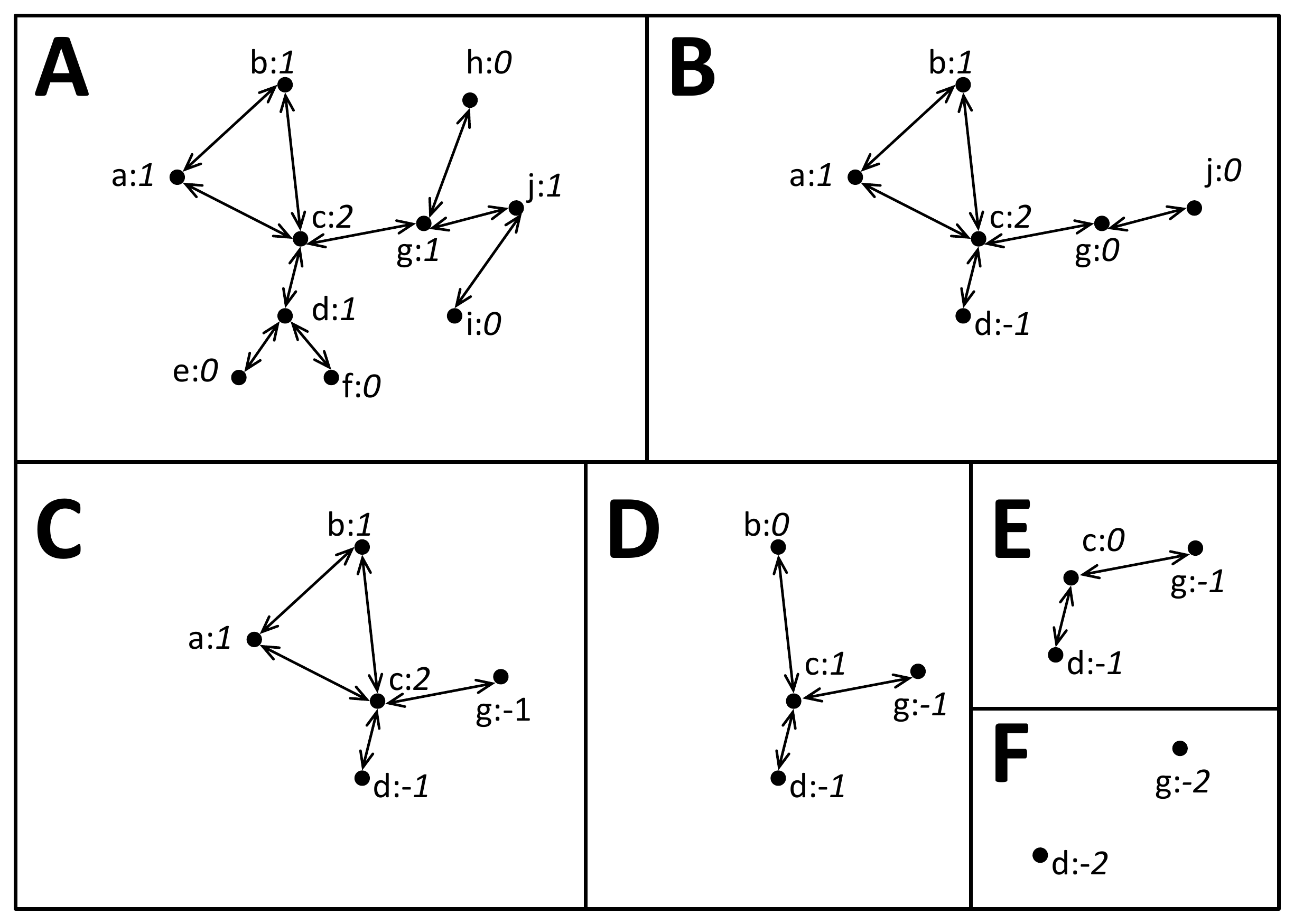
Figure 1: Example of our algorithm for a simple network depicted in box A. We use a threshold value set to $50\%$ of the node degree. Next to each node label (lower-case letter) is the value for $d^{in}_{i}-k_{i}$ (where $k_{i}=\lceil\frac{d^{in}_{i}}{2}\rceil$). In the first four iterations, nodes e, f, h, and i are removed resulting in the network in box B. This is followed by the removal of node j resulting in the network in box C. In the next two iterations, nodes a and b are removed (boxes D-E respectively). Finally, node c is removed (box F). The nodes of the final network, consisting of d and g, have negetive values for $d_{i}-\theta_{i}$ and become the output of the algorithm.

Now, we prove that the resulting set of nodes is guaranteed to cause all nodes in the graph to activate under the tipping model. This proof follows from the fact that any node removed is activated by the remaining nodes in the network.

Theorem 3.1

If all nodes in $V^{\prime}\ \subseteq\ V$ returned by TIP_DECOMP are initially active, then every node in $V$ will eventually be activated, too.

Proof

Let $w$ be the total number of nodes removed by TIP_DECOMP, where $v_{1}$ is the last node removed and $v_{w}$ is the first node removed. We prove the theorem by induction on $w$ as follows. We use $P(w)$ to denote the inductive hypothesis which states that all nodes from $v_{1}$ to $v_{w}$ are active. In the base case, $P(1)$ trivially holds as we are guaranteed that from set $V^{\prime}$ there are at least $k_{1}$ edges to $v_{1}$ (or it would not be removed). For the inductive step, assuming $P(w)$ is true, when $v_{w+1}$ was removed from the graph $dist_{w+1}\geq 0$ which means that $d_{w+1}^{in}\geq k_{w+1}$. All nodes in $\eta^{in}_{w+1}$ at the time when $v_{w+1}$ was removed are now active, so $v_{w+1}$ will now be activated - which completes the proof.

We also note that by using the appropriate data structure (we used a binomial heap in our implementation), for a network of $n$ nodes and $m$ edges, this algorithm can run in time $O(m\log n)$.

Proposition 3

The complexity of TIP_DECOMP is $O(m\cdot log(n))$.

Proof

If we use a binomial heap as described in cormen , we can create a heap where we store each node and assign it a key value of $dist_{i}$ for each node $v_{i}$. The creation of a heap takes constant time and inserting the $n$ vertices will take $O(nlog(n))$ time. We can also maintain a list data structure as well. In the course of the while loop, all nodes will either be removed (as per the algorithm), decreased in key-value no more than $d^{in}_{i}$ or increased to infinity (which we can implement as being removed and added to the list). Hence, the number of decrease key or removal operations is bounded by $n+\sum_{i}d^{in}_{i}$. As $\sum_{i}d^{in}_{i}=m$ (where $m$ is the number of edges). As $O(m\cdot log(n))$, the statement follows.

4 Results

In this section we describe the results of our experimental evaluation. We describe the datasets we used for the experiments in Section 4.1. We evaluate the run-time of TIP_DECOMP in Section 4.1.5. In Section 4.1.6, we evaluate the size of the seed-set returned by the algorithm and we compare this to the seed size returned by known centrality measures in Section 4.2. The speed of the activiation process initiated with seed sets discovered by our algorithm is described in Section 4.3. We then study how the removal of high-degree nodes and community structure affect the results of the algorithm in Sections 4.4 and 4.4.1 respectively.

The algorithm TIP_DECOMP was written using Python 2.6.6 in 200 lines of code that leveraged the NetworkX library available from
http://networkx.lanl.gov/. The code used a binomial heap library written by Björn B. Brandenburg available from http://www.cs.unc.edu/$\sim$bbb/. The experiments were run on a computer equipped with an Intel X5677 Xeon Processor operating at 3.46 GHz with a 12 MB Cache running Red Hat Enterprise Linux version 6.1 and equipped with 70 GB of physical memory. All statistics presented in this section were calculated using R 2.13.1.

4.1 Datasets

In total, we examined $36$ networks: nine academic collaboration networks, three e-mail networks, and $24$ networks extracted from social-media sites. The sites included included general-purpose social-media (similar to Facebook or MySpace) as well as special-purpose sites (i.e. focused on sharing of blogs, photos, or video).

All datasets used in this paper were obtained from one of four sources: the ASU Social Computing Data Repository, Zafarani+Liu:2009 the Stanford Network Analysis Project, snap the University of Michigan, umich and Universitat Rovira i Virgili.uvi $31$ of the networks considered were symmetric – i.e. if a directed edge from vertex $v$ to $v^{\prime}$ exists, there is also an edge from vertex $v^{\prime}$ to $v$. Tables 1 (A-C) show some of the pertinent qualities of the symmetric networks. The networks are categorized by the results for the MIN-SEED experiments (explained later in this section). Additionally, we also looked at several non-symmetric (directed) networks and placed them in their own category. In what follows, we provide their real-world context.

4.1.1 Category A

• BlogCatalog is a social blog directory that allows users to share blogs with friends. Zafarani+Liu:2009 The first two samples of this site, BlogCatalog1 and 2, were taken in Jul. 2009 and June 2010 respectively. The third sample, BlogCatalog3 was uploaded to ASU’s Social Computing Data Repository in Aug. 2010.

• Buzznet is a social media network designed for sharing photographs, journals, and videos. Zafarani+Liu:2009 It was extracted in Nov. 2010.

• Douban is a Chinese social medial website designed to provide user reviews and recommendations. Zafarani+Liu:2009 It was extracted in Dec. 2010.

• Flickr is a social media website that allows users to share photographs. Zafarani+Liu:2009 It was uploaded to ASU’s Social Computing Data Repository in Aug. 2010.

• Flixster is a social media website that allows users to share reviews and other information about cinema. Zafarani+Liu:2009 It was extracted in Dec. 2010.

• FourSquare is a location-based social media site. Zafarani+Liu:2009 It was extracted in Dec. 2010.

• Frienster is a general-purpose social-networking site. Zafarani+Liu:2009 It was extracted in Nov. 2010.

• Last.Fm is a music-centered social media site. Zafarani+Liu:2009 It was extracted in Dec. 2010.

• LiveJournal is a site designed to allow users to share their blogs. Zafarani+Liu:2009 It was extracted in Jul. 2010.

• Livemocha is touted as the “world’s largest language community.” Zafarani+Liu:2009 It was extracted in Dec. 2010.

• WikiTalk is a network of individuals who set and received messages while editing WikiPedia pages. snap It was extracted in Jan. 2008.

4.1.2 Category B

• Delicious is a social bookmarking site, designed to allow users to share web bookmarks with their friends. Zafarani+Liu:2009 It was extracted in Dec. 2010.

• Digg is a social news website that allows users to share stories with friends. Zafarani+Liu:2009 It was extracted in Dec. 2010.

• EU E-Mail is an e-mail network extracted from a large European Union research institution. snap It is based on e-mail traffic from Oct. 2003 to May 2005.

• Hyves is a popular general-purpose Dutch social networking site. Zafarani+Liu:2009 It was extracted in Dec. 2010.

• Yelp is a social networking site that allows users to share product reviews. Zafarani+Liu:2009 It was extracted in Nov. 2010.

4.1.3 Category C

• CA-AstroPh is a an academic collaboration network for Astro Physics from Jan. 1993 - Apr. 2003. snap

• CA-CondMat is an academic collaboration network for Condense Matter Physics. Samples from 1999 (CondMat99), 2003 (CondMat03), and 2005 (CondMat05) were obtained from the University of Michigan. umich A second sample from 2003 (CondMat03a) was obtained from Stanford University. snap

• CA-GrQc is a an academic collaboration network for General Relativity and Quantum Cosmology from Jan. 1993 - Apr. 2003. snap

• CA-HepPh is a an academic collaboration network for High Energy Physics - Phenomenology from Jan. 1993 - Apr. 2003. snap

• CA-HepTh is a an academic collaboration network for High Energy Physics - Theory from Jan. 1993 - Apr. 2003. snap

• CA-NetSci is a an academic collaboration network for Network Science from May 2006.

• Enron E-Mail is an e-mail network from the Enron corporation made public by the Federal Energy Regulatory Commission during its investigation. snap

• URV E-Mail is an e-mail network based on communications of members of the University Rovira i Virgili (Tarragona). uvi It was extracted in 2003.

• YouTube is a video-sharing website that allows users to establish friendship links. Zafarani+Liu:2009 The first sample (YouTube1) was extracted in Dec. 2008. The second sample (YouTube2) was uploaded to ASU’s Social Computing Data Repository in Aug. 2010.

4.1.4 Non-Symmetric Networks

• Epinions is a consumer review website that allows members to establish directed trust relationships. snap

• WikiVote is a sample of Wikipedia users voting beahavior (who votes for whom). snap

• Slashdot formerly had a feature called “Slashdot Zoo” that allowed users to tag each other as friend or foe. We looked at three samples based on friendship relationships: one sample from 2008 (Slashdot1) and two from 2009 (Slashdot2-Slashdot3). snap

Table 1: Information on the networks in Categories A, B, and C.

Table 2: Information on non-symmetric networks.

4.1.5 Runtime

First, we examined the runtime of the algorithm (see Figure 2 and Table 3). Our experiments aligned well with our time complexity result (Proposition 3). For example, a network extracted from the Dutch social-media site Hyves consisting of $1.4$ million nodes and $5.5$ million directed edges was processed by our algorithm in at most $12.2$ minutes. The often-cited LiveJournal dataset consisting of $2.2$ million nodes and $25.6$ million directed edges was processed in no more than $66$ minutes - a short time to approximate an NP-hard combinatorial problem on a large-sized input.

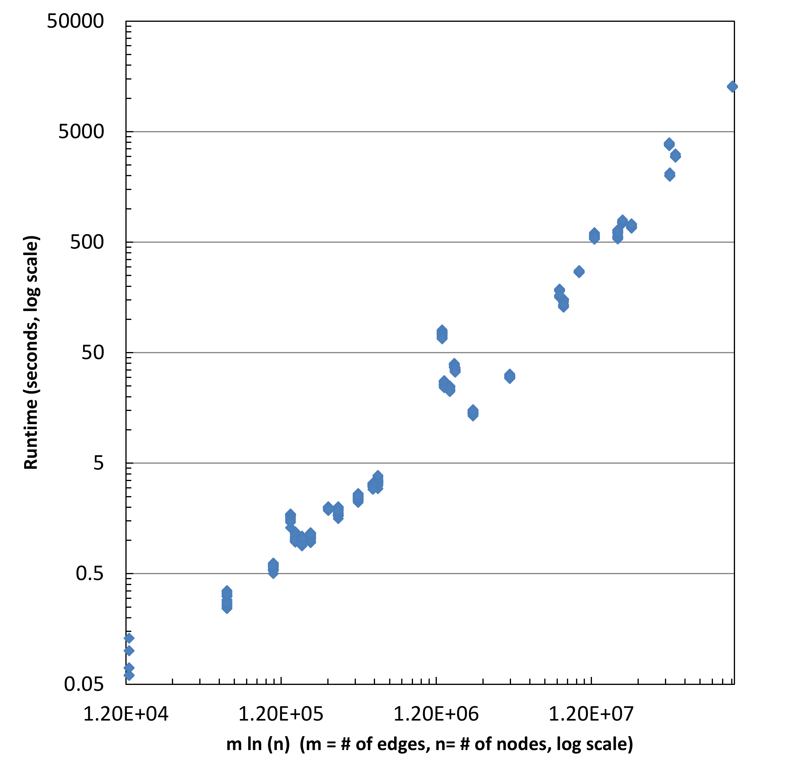
Figure 2: $m\ln n$ vs. runtime in seconds (log scale, $m$ is number of edges, $n$ is number of nodes). The relationship is linear with $R^{2}=0.9015$, $p=2.2\cdot 10^{-16}$.

Table 3: Runtime data on the datasets used in the experiments.

4.1.6 Seed Size

For each network, we performed $10$ “integer” trials. In these trials, we set $\theta(v_{i})=\min(d^{in}_{i},k)$ where $k$ was kept constant among all vertices for each trial and set at an integer in the interval $[1,10]$. We evaluated the ability of a network to promote spreading under the tipping model based on the size of the set of nodes returned by our algorithm (as a percentage of total nodes). For purposes of discussion, we have grouped our networks into three categories based on results (Figure 3 and Table 4). We have also included results for symmetric networks (Figure 4 and Table 5). In general, online social networks had the smallest seed sets - $13$ networks of this type had an average seed set size less than $2\%$ of the population (these networks were all in Category A). We also noticed, that for most networks, there was a linear realtion between threshold value and seed size.

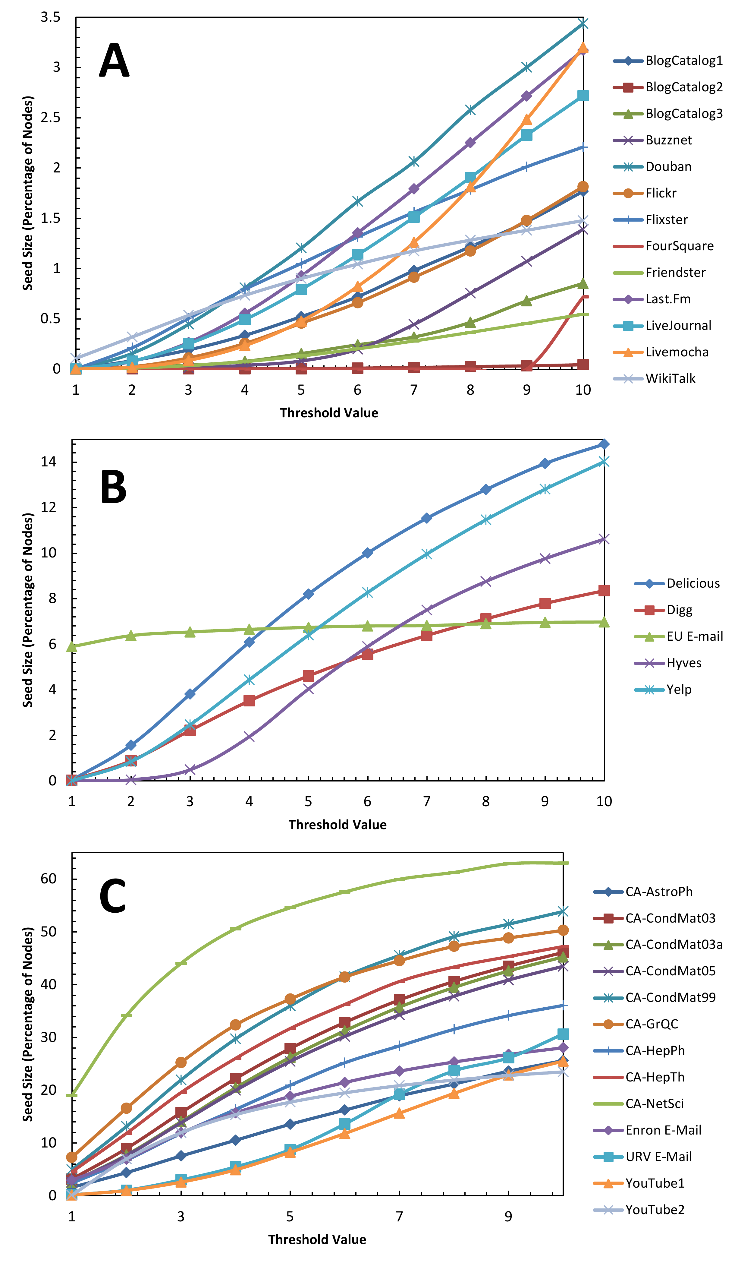
Figure 3: Threshold value (assigned as an integer in the interval $[1,10]$) vs. size of initial seed set as returned by our algorithm in our three identified categories of networks (categories A-C are depicted in panels A-C respectively). Average seed sizes were under $2\%$ for Categorty A, $2-10\%$ for Category B and over $10\%$ for Category C. The relationship, in general, was linear for categories A and B and lograthimic for C. CA-NetSci had the largest Louvain Modularity and clustering coefficient of all the networks. This likely explains why that particular network seems to inhibit spreading.

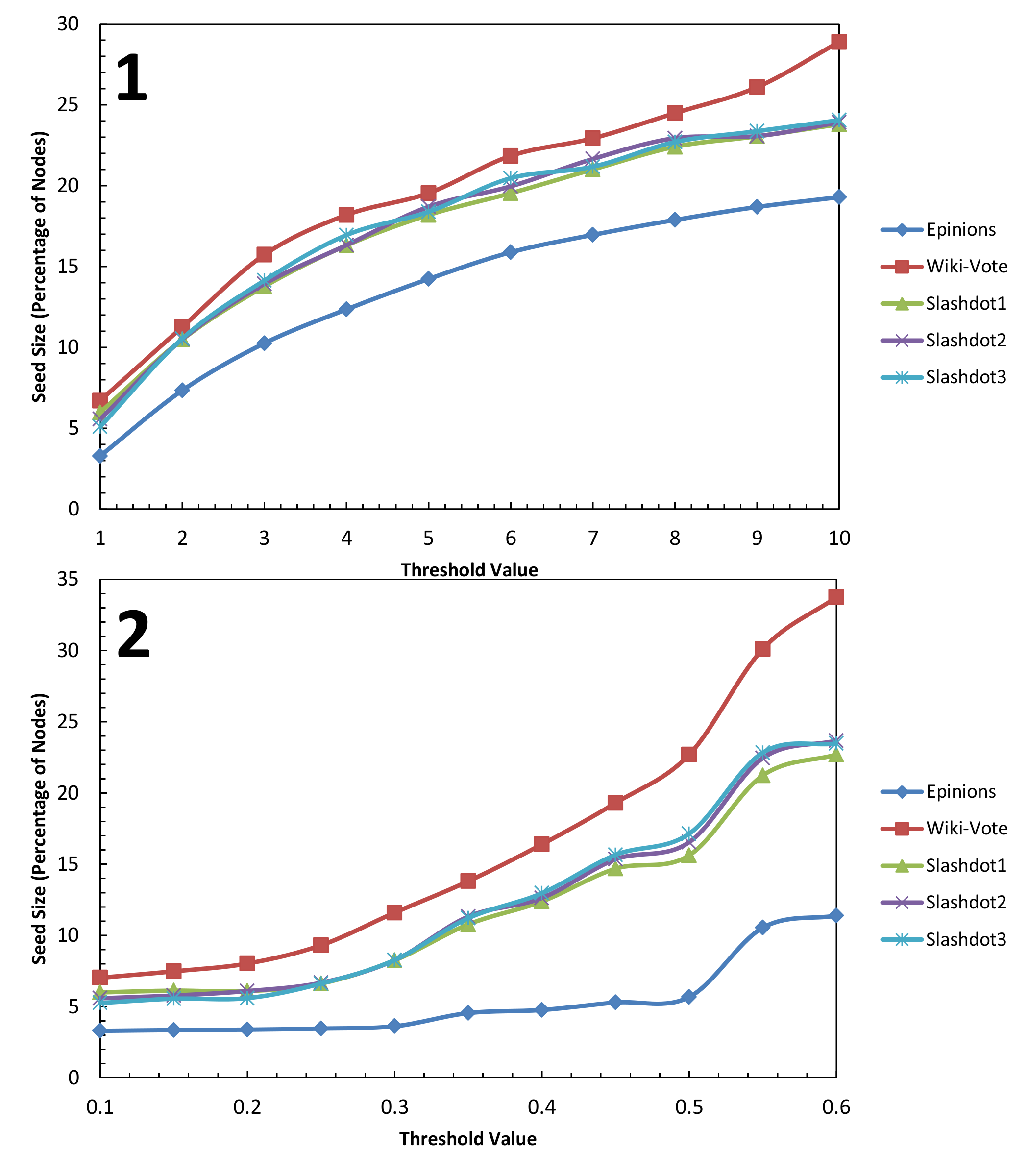
Figure 4: Threshold value assigned as both an integer in the range $[1,10]$ (panel 1) as well as a fraction of node degree (panel 2) for the non-symmetric networks.

Category A can be thought of as social networks highly susceptible to influence - as a very small fraction of initially activated individuals can lead to activation of the entire population. All were extracted from social media websites. For some of the lower threshold levels, the size of the set of seed nodes was particularly small. For a threshold of three, $11$ of the Category A networks produced seeds smaller than $0.5\%$ of the total populationa. For a threshold of four, nine networks met this criteria.

Networks in Category B are susceptible to influence with a relatively small set of initial nodes - but not to the extent of those in Category A. They had an average initial seed size greater than $2\%$ but less than $10\%$. Members in this group included two general purpose social media networks, two specialty social media networks, and an e-mail network. Non-symmetric networks generally perofrmed somewhat poorer than Category B networks (though in general, not as poorly as those in Category C). The initial seed sizes for the non-symmmetric networks ranged from $3\%$ to $29\%$.

Category C consisted of networks that seemed to hamper diffusion in the tipping model, having an average initial seed size greater than $10\%$. This category included all of the academic collaboration networks, two of the email networks, and two networks derived from friendship links on YouTube.

We also studied the effects on spreading when the threshold values were assigned as a specific fraction of each node’s in-degree jy05 ; wattsDodds07 , which results in heterogeneous $\theta_{i}$’s across the network. We performed $12$ trials for each network. Thresholds for each trial were based on the product of in-degree and a fraction in the interval $[0.05,0.60]$ (multiples of $0.05$). The results (Figure 5 and Table 4; for non-symmertic networks see Figure 4 and Table 5) were analogous to our integer tests. We also compared the averages over these trials with $M$ and $C$ and obtained similar results as with the other trials (Figure 14 B).

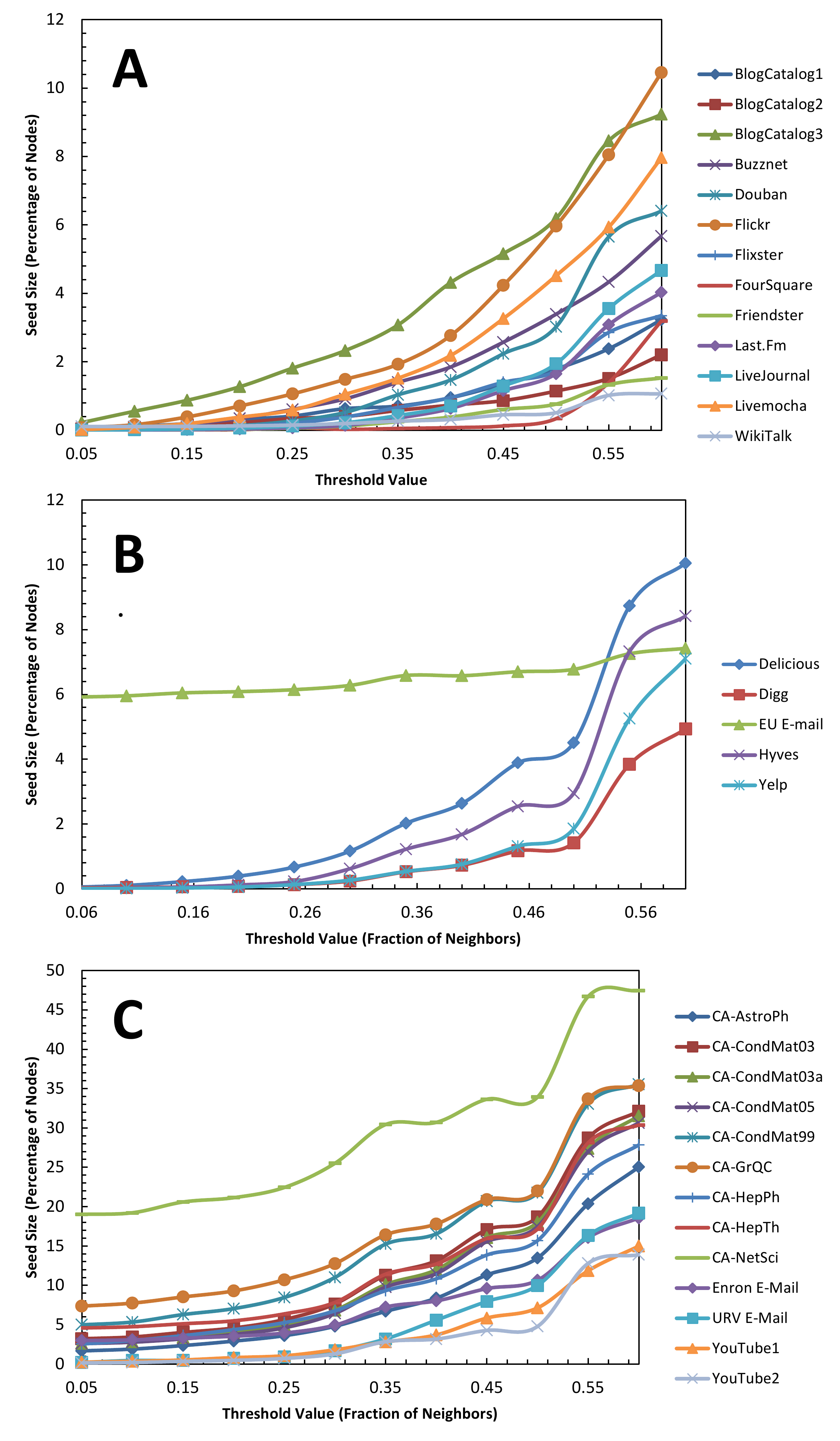
Figure 5: Threshold value (assigned as a fraction of node in-degree as a multiple of $0.05$ in the interval $[0.05,0.60]$) vs. size of initial seed set as returned by our algorithm in our three identified categories of networks (categories A-C are depicted in panels A-C respectively, categories are the same as in Figure 1). Average seed sizes were under $5\%$ for Categorty A, $1-7\%$ for Category B and over $3\%$ for Category C. In general, the relationship between threshold and initial seed size for networks in all categories was exponential.

4.2 Comparison with Centrality Measures

We compared our results with six popular centrality measures: degree, betweenness, closeness, shell number, eigenvector, and PageRank. Here, we define degree centrality is simply the number of outgoing adjacent nodes.  The intuition behind high betweenness centrality nodes is that they function as “bottlenecks” as many paths in the network pass through them. Hence, betweenness is a medial centrality measure. Let $\sigma_{st}$ be the number of shortest paths between nodes $s$ and $t$ and $\sigma_{st}(v)$ be the number of shortest paths between $s$ and $t$ containing node $v$. In freeman77 , betweenness centrality for node $v$ is defined as $\sum_{s\neq v\neq t}\frac{\sigma_{st}(v)}{\sigma_{st}}$. In most implementations, including the ones used in this paper, the algorithm of brandes01 is used to calculate betweenness centrality. Another common measure from the literature that we examined is closeness  freeman79cent . Given node $i$, its closeness $C_{c}(i)$ is the inverse of the average shortest path length from node $i$ to all other nodes in the graph. Intuitively, closeness measures how “close” it is to all other nodes in a network. Formally, if we define the shortest path between nodes $i$ to $j$ as function $d_{G}(i,j)$, we can express the average path length from $i$ to all other nodes as

$$L_{i}=\frac{\sum_{j\in V\setminus i}d_{G}(i,j)}{|V|-1}.$$ (8)

Hence, the closeness of a node can be formally written as

$$C_{c}(i)=\frac{1}{L_{i}}=\frac{|V|-1}{\sum_{j\in V\setminus i}d_{G}(i,j)}.$$ (9)

The idea of shell number is based on a core to which a node lies in. A $c$-core of a network is the subgraph in which every node is connected to the rest of the network by at least $c$ edges. A node is assigned a shell number based on the maximal core that contains it. This value can be derived exactly using shell decomposition Seidman83 . The eigenvector centrality bona72 of a node is assigned based on the associated entry in the eigenvector of the adjacency matrix corresponding to the largest real eigenvalue. The PageRank Page98 for each node based on the PageRank of its neighbors. An initial value for rank is considered for each node and the relationship is then computed iteratively until convergence is reached. Intuitively, PageRank can be thought of as the importance of a node based on the importance of its neighbors. We note that shell number, eigenvector, and PageRank are often associated with diffusion processes. A more complete discussion of centrality measures can be found in wasserman1994social .

We evaluated the performance of centrality measures in finding a seed set by iteratively selecting the most central nodes with respect to a given measure until the $\Gamma_{\theta}$ of that set returns the set of all nodes. Due to the computational overhead of calculating these centrality measures and the repeated re-evaluation of $\Gamma_{\theta}$, we limited this comparison to only BlogCatalog3, CA-HepTh, CA-NetSci, URV E-Mail, and Douban (no betweeness calcualted for Douban). As with the experiments in the previous section, we studied threshold settings based on an integer in the interval $[1,10]$ (see Figure 6) and as a fraction of incoming neighbors in the interval $[0.05,0.60]$ (multiples of $0.05$, see Figure 8). In general, selecting highly-central nodes is an inefficient method for finding small seed sets.

In all but the lowest threshold settings, the use of centrality measures for the integer-threshold trials proved to significantly underperformed when the method presented in this paper - often returning seed-sets several orders of magnitude larger and in many cases including the majority of nodes in the network. Even for the centrality measures outperformed our method in these trials, the reduction in seed set size was minimal (the greatest reduction in seed set size experienced in a centrality-measure test over the algorithm of this paper was $0.09\%$, while often producing seed sets orders of magnitude greater than our method). This held even for the centrality measures associated with diffusion (shell number, eigenvector, and PageRank).

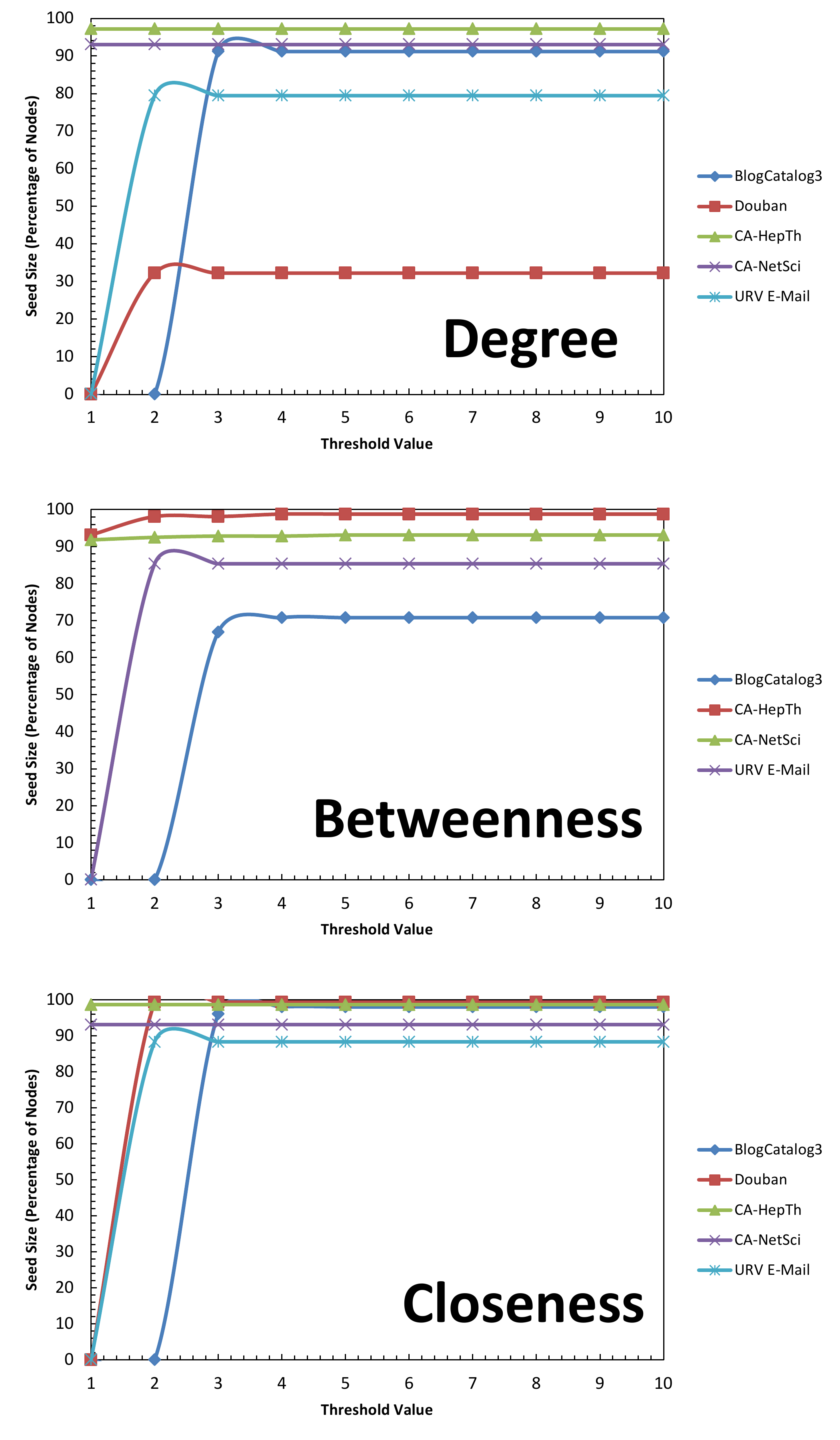
Figure 6: The use of degree, betweenness and closeness to find seed-sets on select networks when the threshold is set to an integer in the interval $[1,10]$. For these trials, centrality measure returned significantly larger (several orders of magnitude) larger seed sets than our approach.

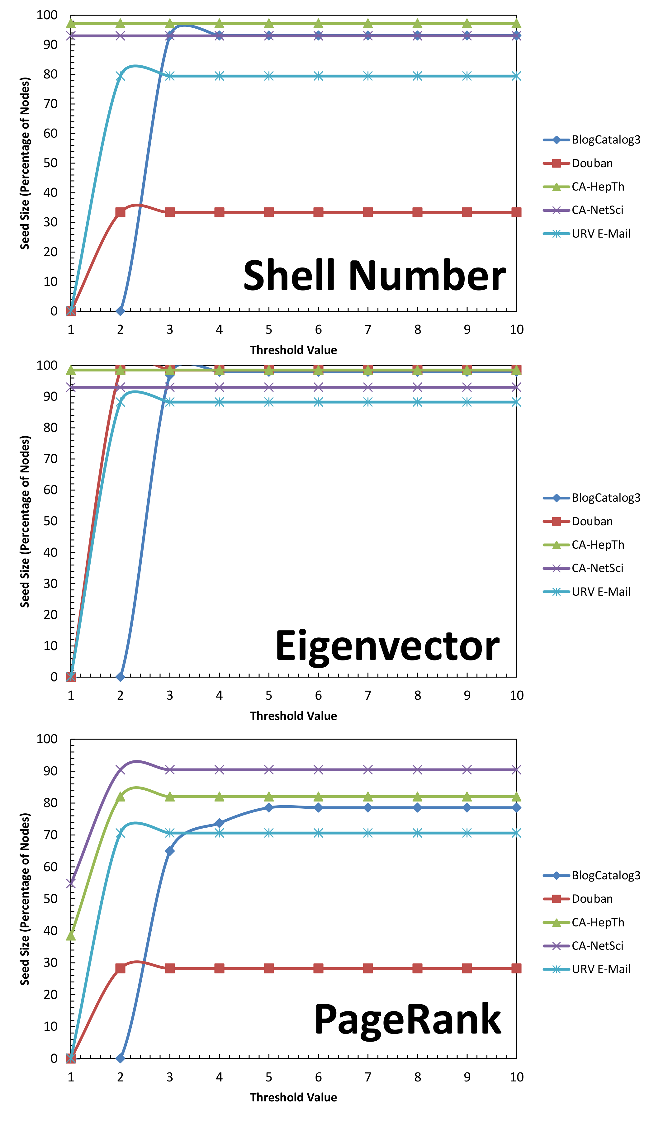
Figure 7: The use of shell number, Eigenvector, and PageRank to find seed-sets on select networks when the threshold is set to an integer in the interval $[1,10]$.

Our tests using fractional-based thresholds tell a slightly different story. While our method still generally outperformed the centrality measures for the fractional tests, there were a few cases where the centrality measures fared better. With BlogCatalog3 all of the centrality measures outperformed our algorithm in the fraction-based experiments. For that dataset, centrality-based algorithm consistently outperformed our method finding seed sets with less members (by $3.13-3.29\%$ of the population, on average). With URV-Email, many trials that utilized a lower threshold setting outperformed our method, but never finding a feed set with smaller by more than $8\%$ of the total population. However, in the larger threshold settings, our method consistently found smaller seeds. For a given centrality measure for this dataset, centrality measures on average provided poorer results than our algorithm ranged - returning seed sets which were, on average $10.22-67.14\%$ (by overall population) larger than that returned by our algorithm. Perhaps the most interesting result among the centrality measures were the PageRank fraction-based tests on CA-NetSci, which is associated with the largest seed sets. PageRank found seed sets that were, on average $14.45\%$ smaller (by population) than our approach. Additionally, though centrality measures outperformed TIP_DECOMP for BlogCatalog3, this does not appear to hold for all social networks as the seed sets returned using centrality measures for the Douban approaches at least an order of magnitude increase over our method for nearly every fractional threshold setting for all centrality measures. Hence, we conclude that for fraction-based thresholds, using centrality measures to find seed sets provides inconsistent results, and when it fails, it tends to provide a large portion of the network. A possibility for a practical algorithm that could combine both methods would be to first run TIP_DECOMP, returning some set $V^{\prime}$. Then, create set $V^{\prime\prime}$ by selecting the most central nodes until either $|V^{\prime}|=|V^{\prime\prime}|$ or $\Gamma_{\theta}(V^{\prime\prime})=V$ (whichever ensures the lower cardinality for $V^{\prime\prime}$. If $|V^{\prime}|=|V^{\prime\prime}|$, return $V^{\prime}$, otherwise return $V^{\prime\prime}$. For such an approach, we would likely recommend using degree centrality due to its ease of computation and performance in our experiments. However, we note that highly-central nodes often may not be realistic targets for a viral-marketing campaign. For instance, it may be cost-prohibitive to create a seed set consisting of major celebrities in order to spread the use of a product. As such is a practical concern, we look at the performance of TIP_DECOMP when high-degree nodes are removed in the next section.

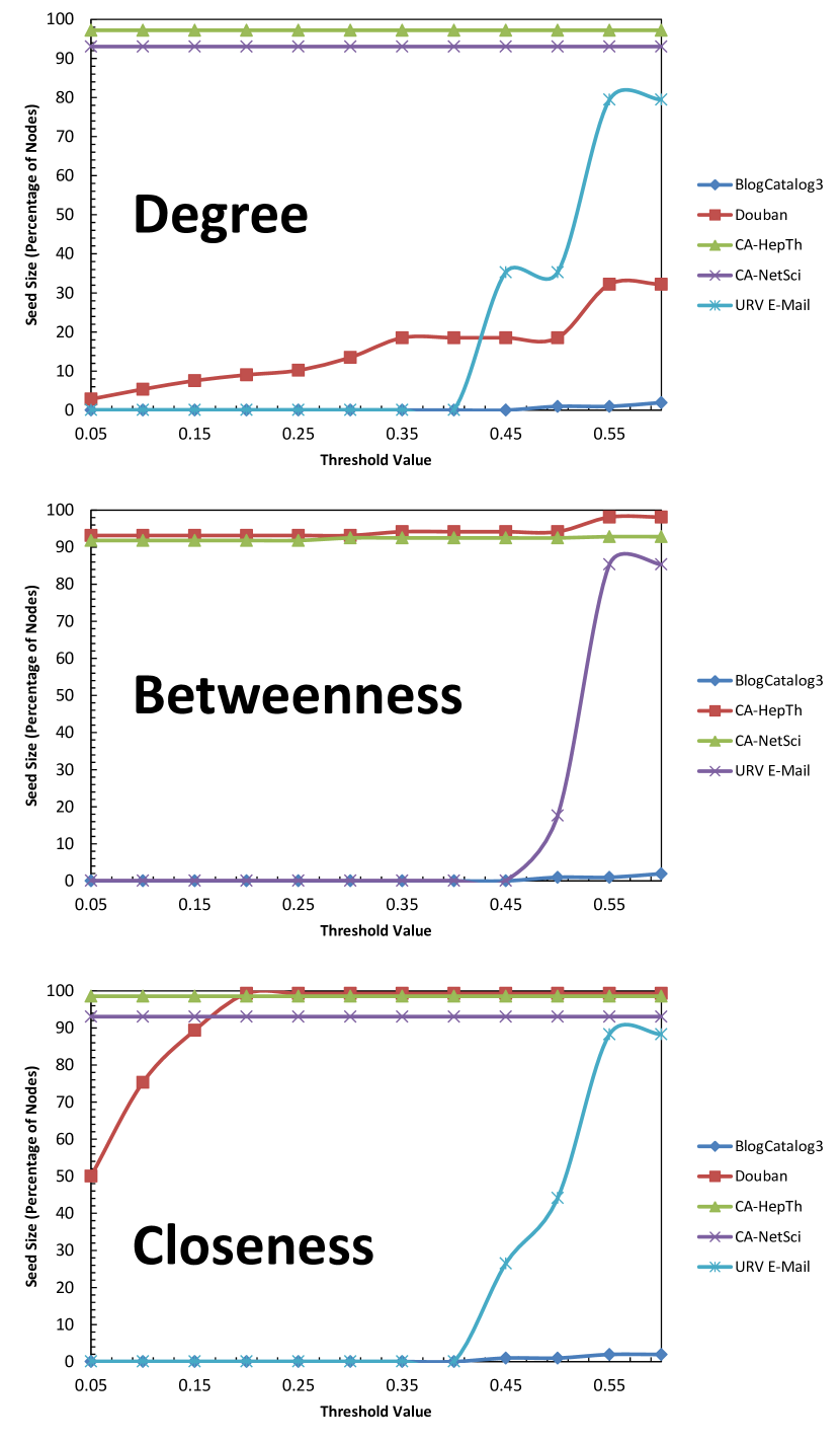
Figure 8: The use of degree, betweenness and closeness to find seed-sets on select networks when the threshold is set to an fraction in the interval $[0.05,0.60]$ (multiples of $0.05$).

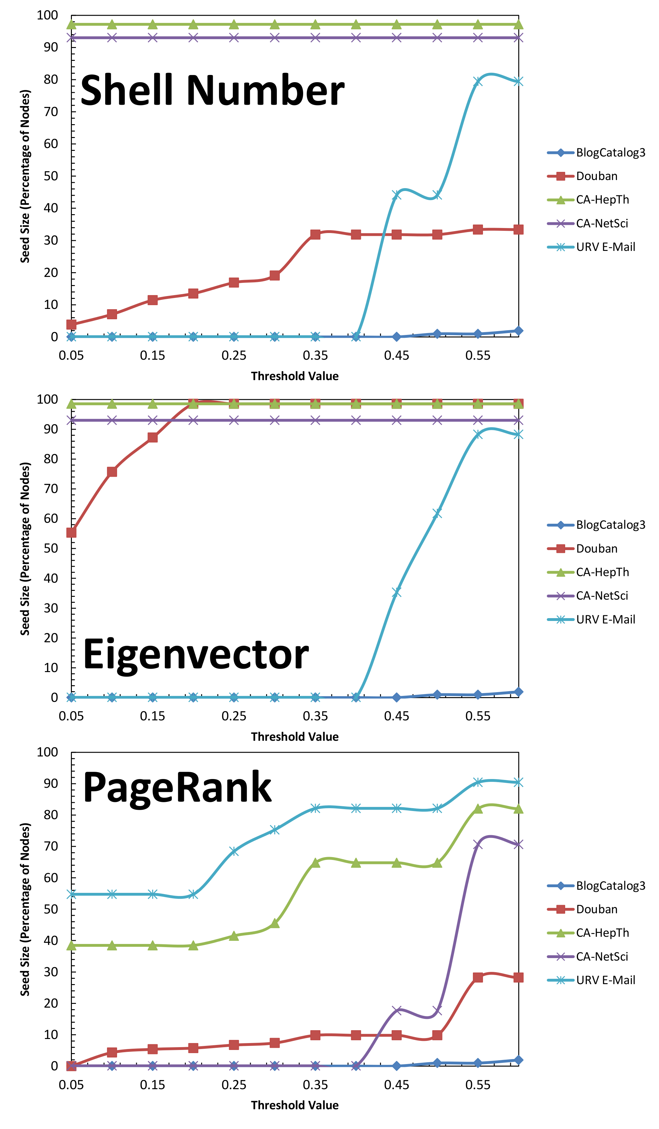
Figure 9: The use of shell number, Eigenvector, and PageRank to find seed-sets on select networks when the threshold is set to an fraction in the interval $[0.05,0.60]$ (multiples of $0.05$).

4.3 The Speed of the Activation Process and Sets of “Critical Mass”

An important aspect to consider in viral marketing is the speed of the activation process. We illustrate this speed for several networks under a threshold of $2$ as well as a majority threshold (half of each nodes neighbors) in Figure 10. Interestingly, we found that the size of the initial seed set was not indicative of the speed of spreading. For instance, in BlogCatalog3, a Category A network (for which our algorithm found a very small seed set) the activation process proceeded quickly when compared to the others examined. However, this was also true for CA-NetSci, a Category C network (large seed set). Conversely, the activation process in the Douban and CA-HepTh networks (also Category A and C, respectively) proceeded more slowly than the rest.

Another interesting feature we learned in exploring the speed of the activation process was that in all of our experiments there was a single time step where the number of activated nodes increased significantly more than the other time periods - sometimes by several orders of magnitude (see Figure 11). We can think of such a set of activated nodes as when the population reaches a “critical mass” which results in mass adoption in the next interval. In many cases, such a critical mass is reached early - normally in the first few time-steps.

Finding a subset of the population of “critical mass” may be an important problem in its own right. Though the critical mass point will often be larger than the seed set found by an algorithm in this paper, we can be assured that in one time step of the model, the number of individuals reached (with a certain number of signals from their neighbors) is substantially larger than the investment. In practice, this could lead to quicker spreading of information in an advertising campaign, for example. Further, our experiments indicate that order-of-magnitude critical mass sets exist in several networks. We are currently conducting further research on this topic.

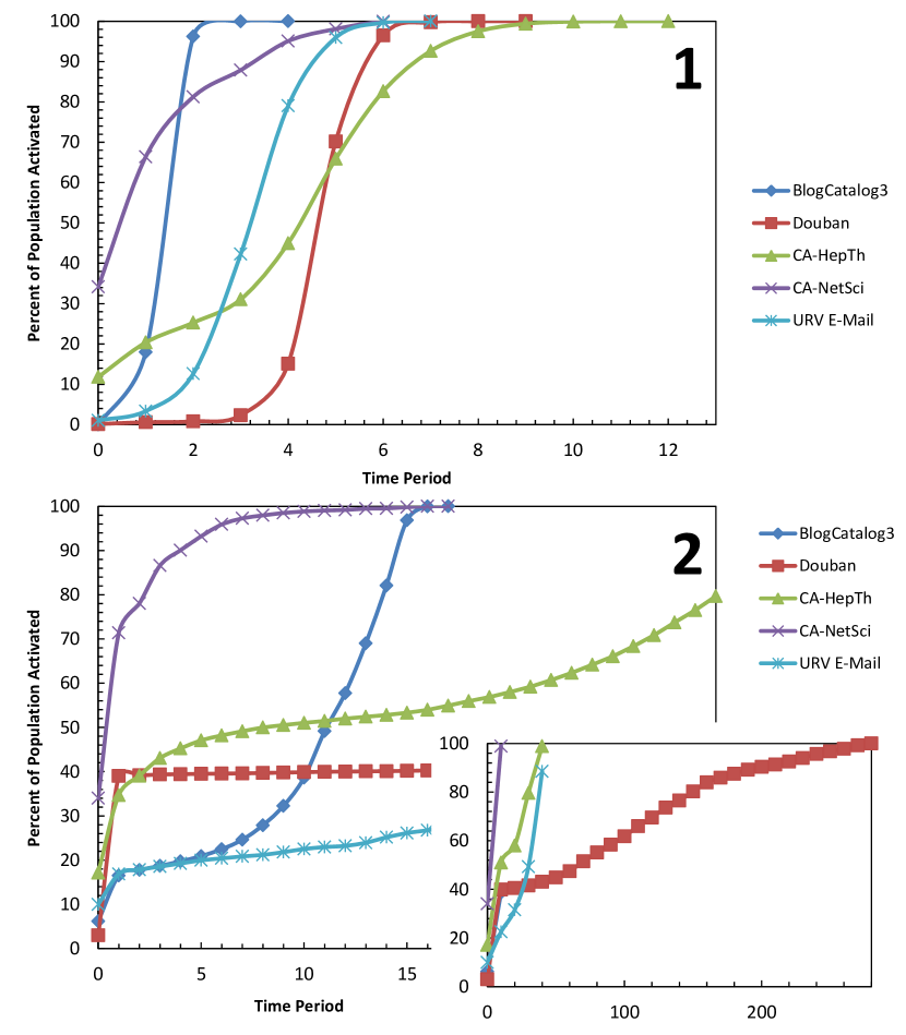
Figure 10: An examination of several of speed of activation initiated from the seed set using a threshold of two (panel 1) and a majority threshold (panel 2).

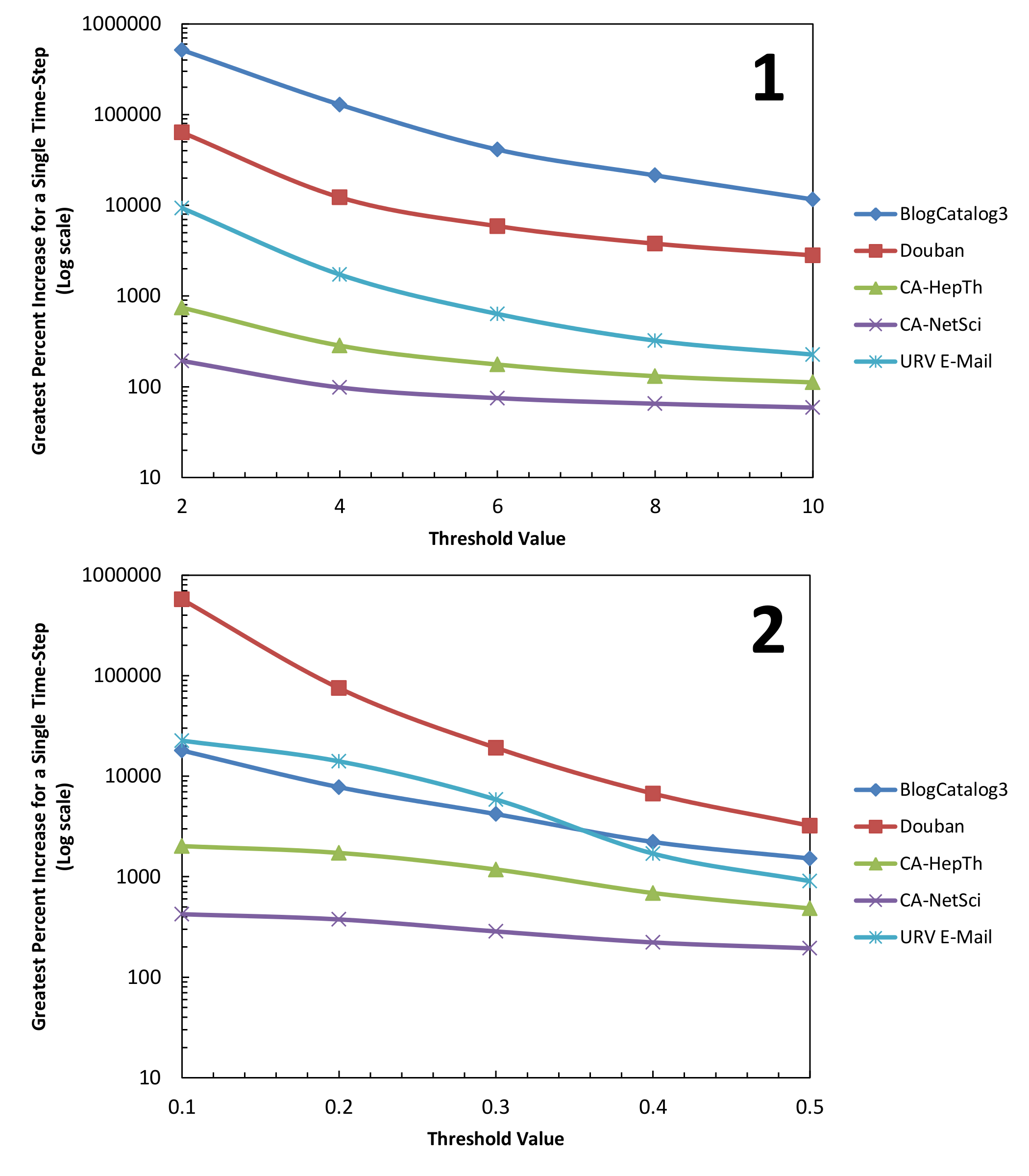
Figure 11: Greatest Percent increase experienced in a single time step (the effect of reaching “critical mass”) for integer-based and percentage-based thresholds (panel 1 and 2 respectively).

4.4 Effect of Removing High-Degree Nodes

In the last section we noted that high-degree nodes may not always be targetable in a viral marketing campaign (i.e. it may be cost prohibitive to include them in a seed set). In this section, we explore the affect of removing high-degree nodes on the size of the seed-set returned by TIP_DECOMP. This type of node removal has also recently been studied in a different context in nodeRemRef . In these trials, we studied all $31$ networks and looked at two specific threshold settings: an integer threshold of $2$ (Figure 12) and a fractional threshold of $0.5$ (Figure 13). We then studied the effect of removing up to $50\%$ of the nodes in order from greatest to least degree.

With an integer threshold of $2$, networks in category A still retained a seed-size (as returned by TIP_DECOMP) two orders of magnitude smaller than the population size up to the removal of $10\%$ of the top degree nodes, and for many networks this was maintained to $50\%$. Networks in category B retained seed sets an order of magnitude smaller than the population for up to $50\%$ of the nodes removed. For most networks in category C, the seed size remained about a quarter of the population size up to $15\%$ of the top degree nodes being removed.

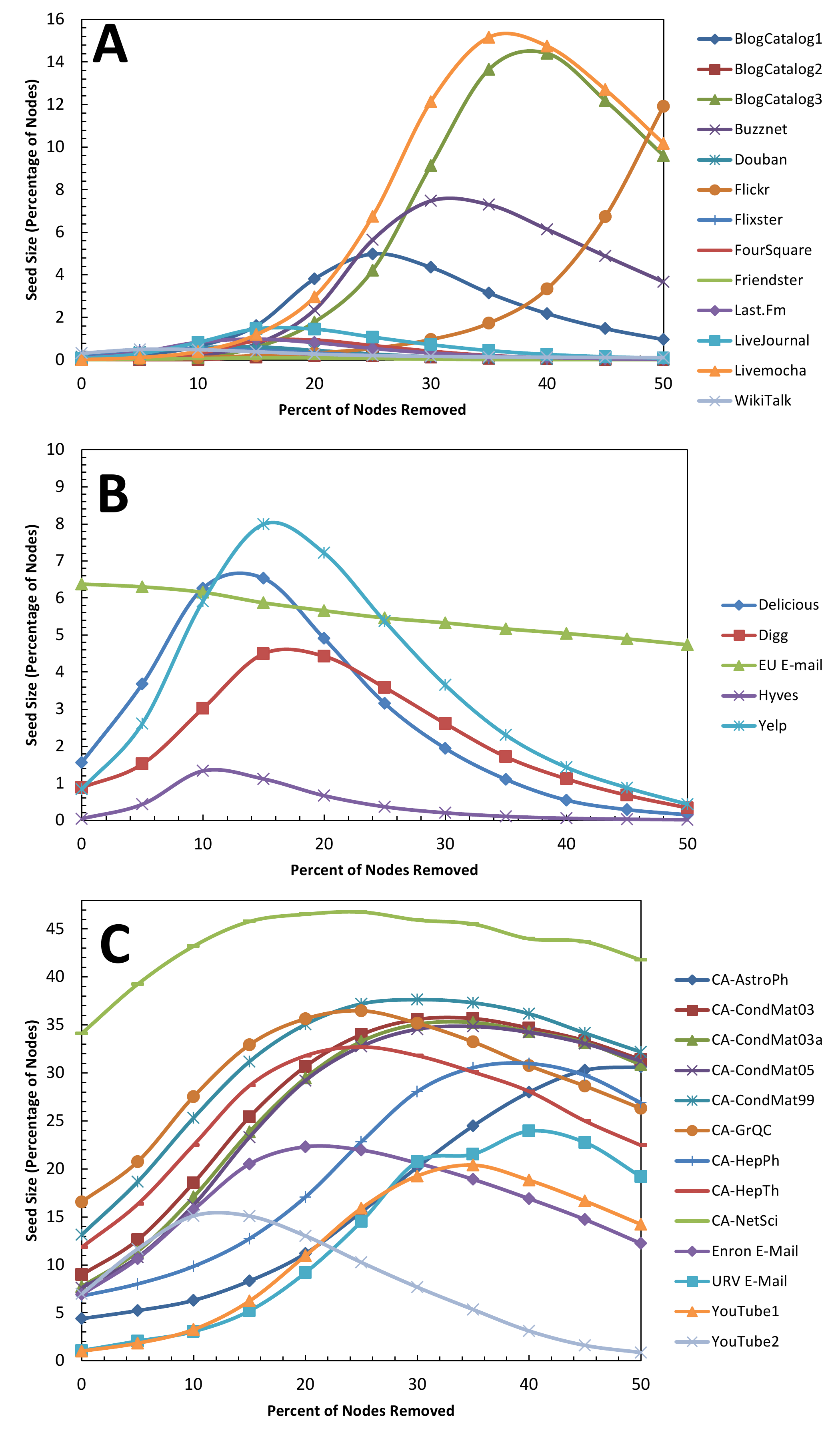
Figure 12: Size of the seed set returned by TIP_DECOMP (as a fraction of the popualtion) as a function of the percent of the highest degree nodes removed from the network with an integer theshold of $2$ for networks in categories A-C.

With a fractional threshold of $0.5$, we noted that many networks in category A actually had larger seed sets (as returned by TIP_DECOMP) when more high degree nodes are removed. Further, networks in categories A-B retained seed sets of at least an order of magnitude smaller than the population in these tests while most networks in category C retained sizes of about a quarter of the population.

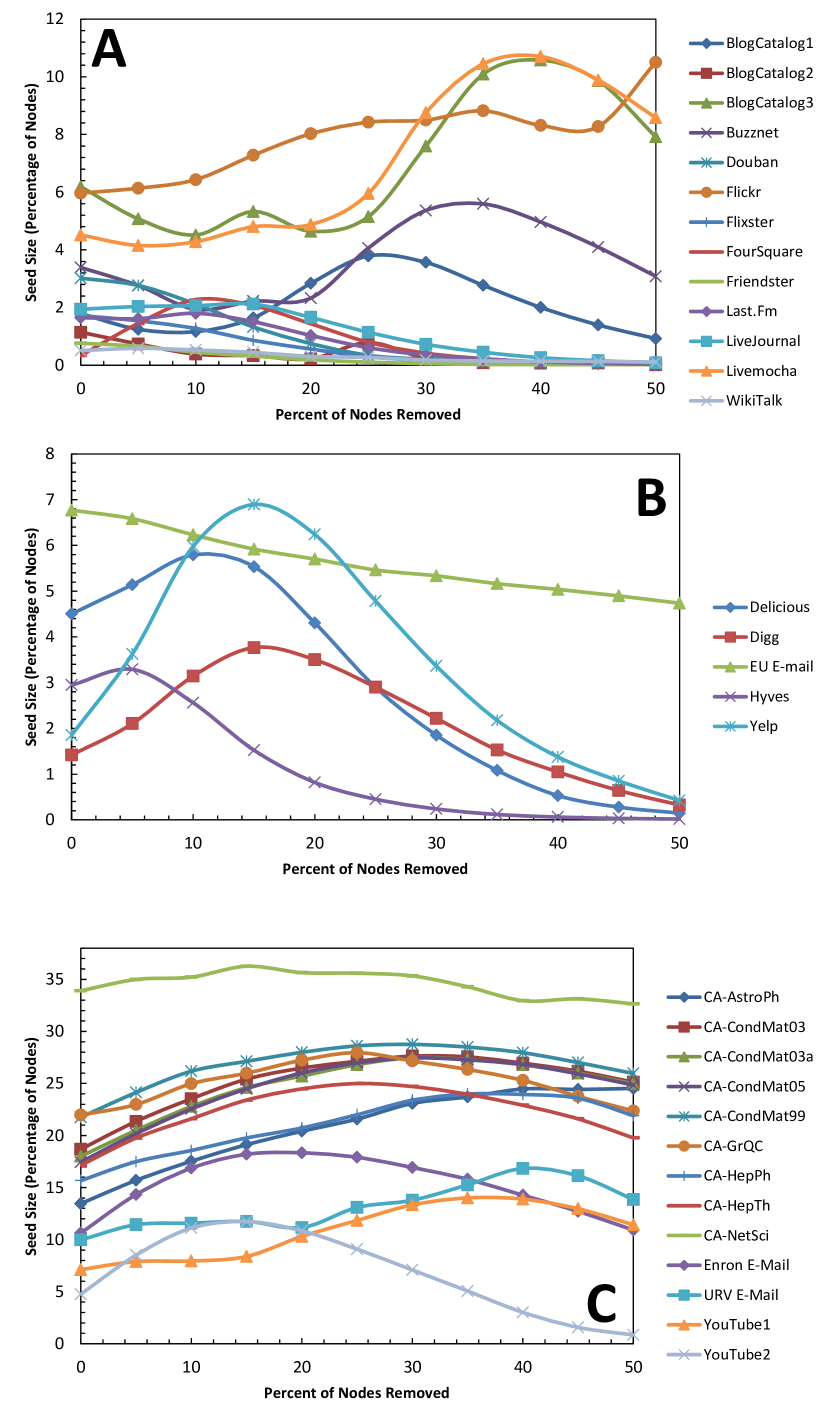
Figure 13: Size of the seed set returned by TIP_DECOMP (as a fraction of the popualtion) as a function of the percent of the highest degree nodes removed from the network with an fractional theshold of $0.5$ for networks in categories A-C.

4.4.1 Seed Size as a Function of Community Structure

In this section, we view the results of our heuristic algorithm as a measurement of how well a given network promotes spreading. Here, we use this measurement to gain insight into which structural aspects make a network more likely to be “tipped.” We compared our results with two network-wide measures characterizing community structure. First, clustering coefficient ($C$) is defined for a node as the fraction of neighbor pairs that share an edge - making a triangle. For the undirected case, we define this concept formally below.

Definition 7 (Clustering Coefficient)

Let $r$ be the number of edges between nodes with which $v_{i}$ has an edge and $d_{i}$ be the degree of $v_{i}$. The clustering coefficient, $C_{i}=\dfrac{2r}{d_{i}(d_{i}-1)}$.

Intuitively, a node with high $C_{i}$ tends to have more pairs of friends that are also mutual friends. We use the average clustering coefficient as a network-wide measure of this local property.

Second, we consider modularity ($M$) defined by Newman and Girvan. newman04 . For a partition of a network, $M$ is a real number in $[-1,1]$ that measures the density of edges within partitions compared to the density of edges between partitions. We present a formal definition for an undirected network below.

Definition 8 (Modularity newman04 )

Given partition $C=\{c_{1},\ldots,c_{q}\}$, modularity,

$$M=\dfrac{1}{2m}\sum_{c\in C}\sum_{i,j\in c}w_{ij}-P_{ij}$$

where $m$ is the number of undirected edges; $w_{ij}=1$ if there is an edge between nodes $i$ and $j$ and $w_{ij}=0$ otherwise; $P_{ij}=\frac{k_{i}k_{j}}{2m}$

The modularity of an optimal network partition can be used to measure the quality of its community structure. Though modularity-maximization is NP-hard, the approximation algorithm of Blondel et al. blondel08 (a.k.a. the “Louvain algorithm”) has been shown to produce near-optimal partitions. We call the modularity associated with this algorithm the “Louvain modularity.” Unlike the $C$, which describes local properties, $M$ is descriptive of the community level. For the $31$ networks we considered, $M$ and $C$ appear uncorrelated ($R^{2}=0.0538$, $p=0.2092$).

We plotted the initial seed set size ($S$) (from our algorithm - averaged over the $10$ threshold settings) as a function of $M$ and $C$ (Figure 14a) and uncovered a correlation (planar fit, $R^{2}=0.8666$, $p=5.666\cdot 10^{-13}$, see Figure 14 A). The majority of networks in Category C (less susceptible to spreading) were characterized by relatively large $M$ and $C$ (Category C includes the top nine networks w.r.t. $C$ and top five w.r.t. $M$). Hence, networks with dense, segregated, and close-knit communities (large $M$ and $C$) suppress spreading. Likewise, those with low $M$ and $C$ tended to promote spreading. Also, we note that there were networks that promoted spreading with dense and segregated communities, yet were less clustered (i.e. Category A networks Friendster and LiveJournal both have $M\geq 0.65$ and $C\leq 0.13$). Further, some networks with a moderately large clustering coefficient were also in Category A (two networks extracted from BlogCatalog had $C\geq 0.46$) but had a relatively less dense community structure (for those two networks $M\leq 0.33$).

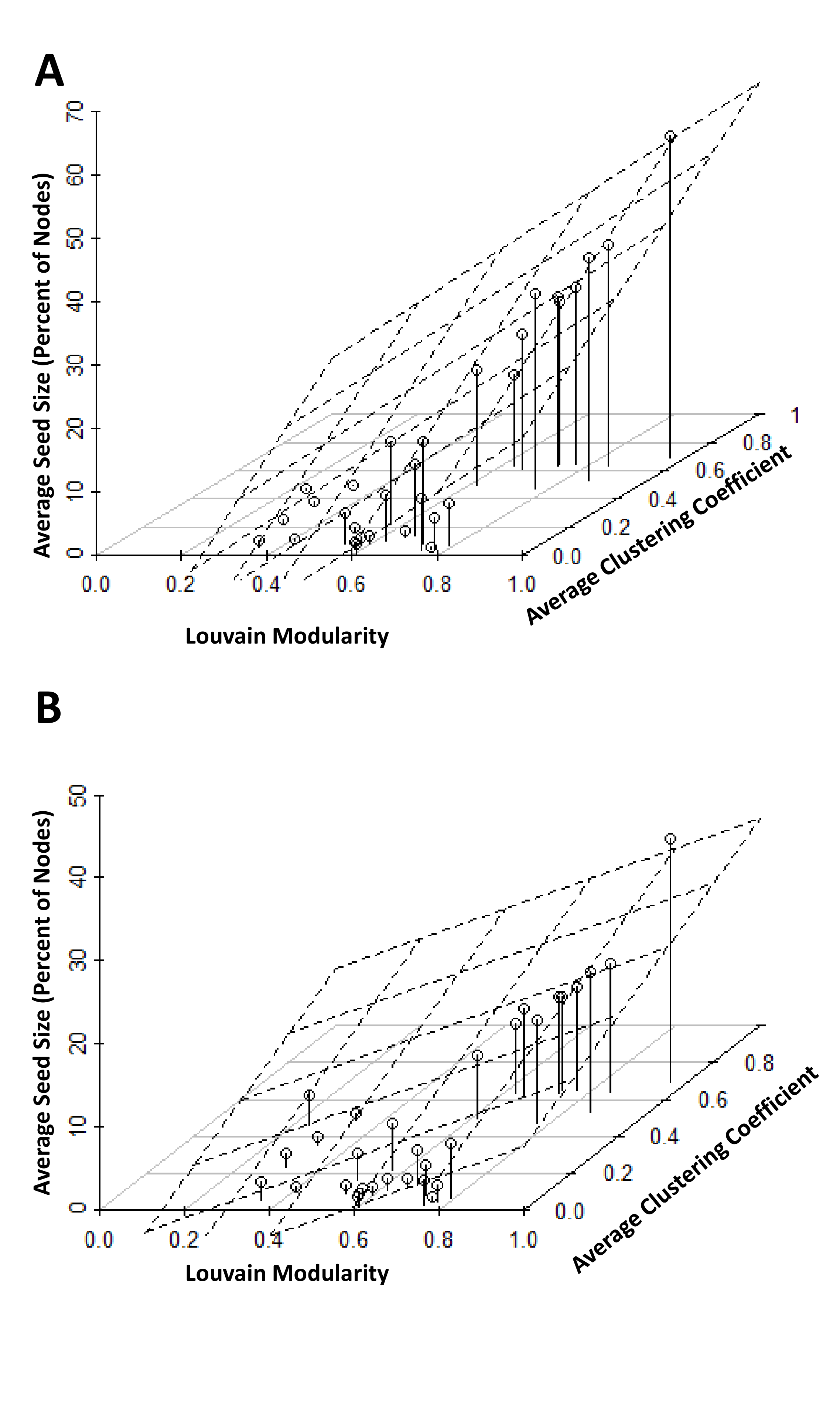
Figure 14: (A) Louvain modularity ($M$) and average clustering coefficient ($C$) vs. the average seed size ($S$). The planar fit depicted is $S=43.374\cdot M+33.794\cdot C-24.940$ with $R^{2}=0.8666$, $p=5.666\cdot 10^{-13}$. (B) Same plot at (A) except the averages are over the 12 percentage-based threshold values. The planar fit depicted is $S=18.105\cdot M+17.257\cdot C-10.388$ with $R^{2}=0.816$, $p=5.117\cdot 10^{-11}$.

Table 4: Regression analysis and network-wide measures for the networks in Categories A, B, and C.

Table 5: Regression analysis and network-wide measures for the non-symmetric networks.

5 Related Work

Tipping models first became popular by the works of Gran78 and Schelling78 where it was presented primarily in a social context. Since then, several variants have been introduced in the literature including the non-deterministic version of kleinberg (described later in this section) and a generalized version of jy05 . In this paper we focused on the deterministic version. In wattsDodds07 , the authors look at deterministic tipping where each node is activated upon a percentage of neighbors being activated. Dryer and Roberts Dreyer09 introduce the MIN-SEED problem, study its complexity, and describe several of its properties w.r.t. certain special cases of graphs/networks. The hardness of approximation for this problem is described in chen09siam . The work of benzwi09 presents an algorithm for target-set selection whose complexity is determined by the tree-width of the graph - though it provides no experiments or evidence that the algorithm can scale for large datasets. The recent work of reichman12 proves a non-trivial upper bound on the smallest seed set.

Our algorithm is based on the idea of shell-decomposition that currently is prevalent in physics literature. In this process, which was introduced in Seidman83 , vertices (and their adjacent edges) are iteratively pruned from the network until a network “core” is produced. In the most common case, for some value $k$, nodes whose degree is less than $k$ are pruned (in order of degree) until no more nodes can be removed. This process was used to model the Internet in ShaiCarmi07032007 and find key spreaders under the SIR epidemic model in InfluentialSpreaders_2010 . More recently, a “heterogeneous” version of decomposition was introduced in baxter11 - in which each node is pruned according to a certain parameter - and the process is studied in that work based on a probability distribution of nodes with certain values for this parameter.

5.1 Notes on Non-Deterministic Tipping

We also note that an alternate version of the model where the thresholds are assigned randomly has inspired approximation schemes for the corresponding version of the seed set problem.kleinberg ; leskovec07 ; chen10 Work in this area focused on finding a seed set of a certain size that maximizes the expected number of adopters. The main finding by Kempe et al., the classic work for this model, was to prove that the expected number of adopters was submodular - which allowed for a greedy approximation scheme. In this algorithm, at each iteration, the node which allows for the greatest increase in the expected number of adopters is selected. The approximation guarantee obtained (less than $0.63$ of optimal) is contingent upon an approximation guarantee for determining the expected number of adopters - which was later proved to be $\#P$-hard. chen10 Recently, some progress has been made toward finding a guarantee Borgs12 . Further, the simulation operation is often expensive - causing the overall time complexity to be $O(x\cdot n^{2})$ where $x$ is the number of runs per simulation and $n$ is the number of nodes (typically, $x>n$). In order to avoid simulation, various heuristics have been proposed, but these typically rely on the computation of geodesics - an $O(n^{3})$ operation - which is also more expensive than our approach.

Additionally, the approximation argument for the non-deterministic case does not directly apply to the original (deterministic) model presented in this paper. A simple counter-example shows that sub-modularity does not hold here. Sub-modularity (diminishing returns) is the property leveraged by Kempe et al. in their approximation result.

5.2 Note on an Upper Bound of the Initial Seed Set

Very recently, we were made aware of research by Daniel Reichman that proves an upper bound on the minimal size of a seed set for the special case of undirected networks with homogeneous threshold values. reichman12 The proof is constructive and yields an algorithm that mirrors our approach (although Reicshman’s algorithm applies only to that special case). We note that our work and the work of Reichman were developed independently. We also note that Reichman performs no experimental evaluation of the algorithm.

Given undirected network $G$ where each node $v_{i}$ has degree $d_{i}$ and the threshold value for all nodes is $k$, Reichman proves that the size of the minimal seed set can be bounded by $\sum_{i}\min\{1,\frac{k}{d_{i}+1}\}$. For our integer tests, we compared our results to Reichman’s bound. Our seed sets were considerably smaller - often by an order of magnitude or more. See Figure 15 for details.

6 Conclusion

As recent empirical work on tipping indicates that it can occur in real social networks,centola10 ; zhang11 our results are encouraging for viral marketers. Even if we assume relatively large threshold values, small initial seed sizes can often be found using our fast algorithm - even for large datasets. For example, with the FourSquare online social network, under majority threshold ($50\%$ of incoming neighbors previously adopted), a viral marketeer could expect a $297$-fold return on investment. As results of this type seem to hold for many online social networks, our algorithm seems to hold promise for those wishing to “go viral.” An important open question to address in future work is if a similar decomposition-based approach is viable for finding seed sets under other diffusion models, such as the independent cascade model kleinberg and evolutionary graph theory lieberman_evolutionary_2005 as well as probabilistic variants of the tipping model and diffusion processes on multi-modal networks snops-iclp . Exploring other models can lead to the development of decomposition algorithms in domains where social behavior is more dynamic such as cell-phone networks dyag13 ; otherPho .

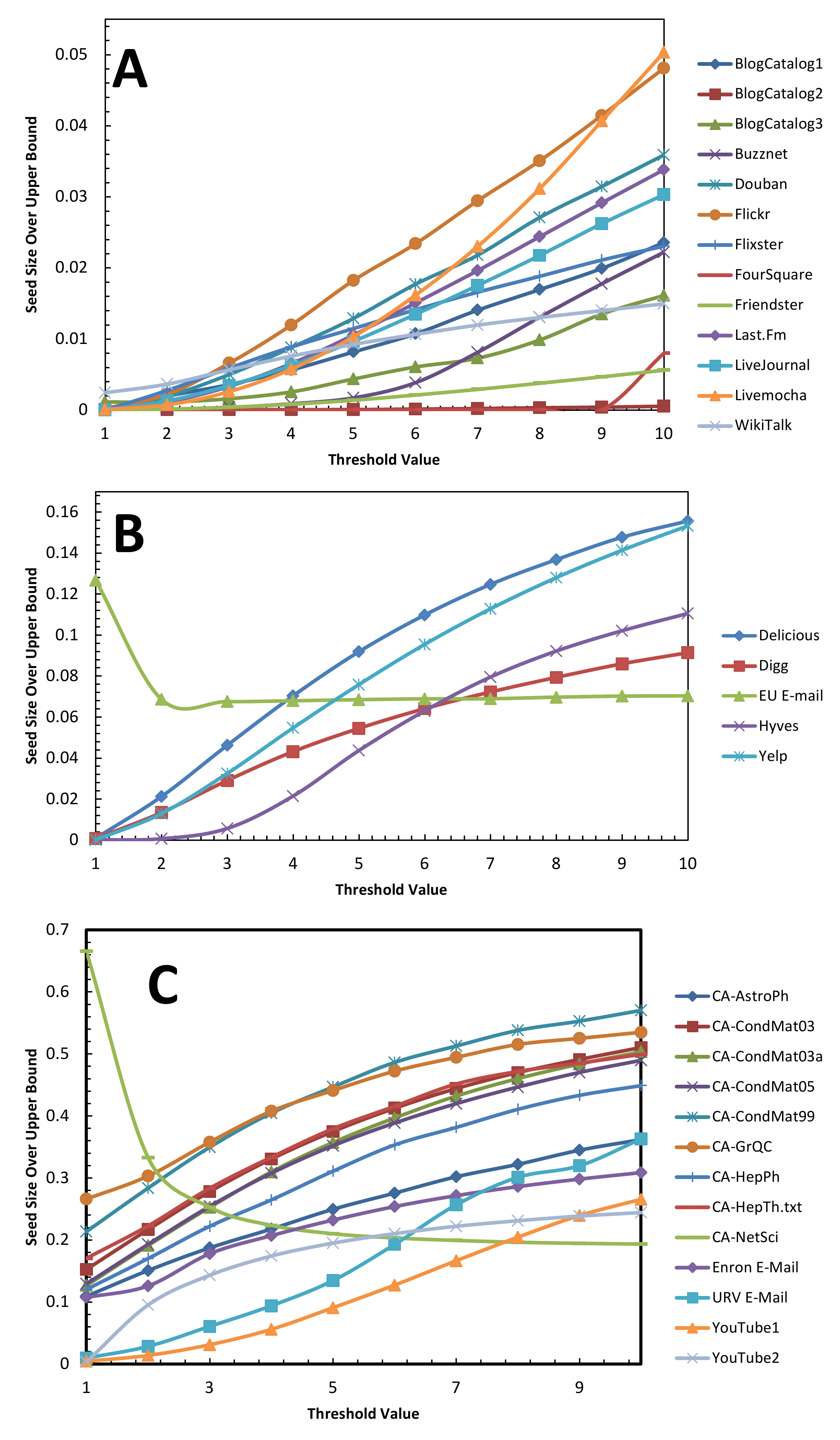
Figure 15: Integer threshold values vs. the seed size divided by Reichman’s upper bound reichman12 the three categories of networks (categories A-C are depicted in panels A-C respectively). Note that in nearly every trial, our algorithm produced an initial seed set significantly smaller than the bound - in many cases by an order of magnitude or more.

References

- (1) Arenas, A.: Network data sets (2012). URL http://deim.urv.cat/ aarenas/data/welcome.htm
- (2) Baxter, G.J., Dorogovtsev, S.N., Goltsev, A.V., Mendes, J.F.F.: Heterogeneous -core versus bootstrap percolation on complex networks. Phys. Rev. E 83 (2011)
- (3) Ben-Zwi, O., Hermelin, D., Lokshtanov, D., Newman, I.: Treewidth governs the complexity of target set selection. Discrete Optimization 8(1), 87–96 (2011)
- (4) Blondel, V., Guillaume, J., Lambiotte, R., Lefebvre, E.: Fast unfolding of communities in large networks. Journal of Statistical Mechanics: Theory and Experiment 2008, P10,008 (2008)
- (5) Boldi, P., Rosa, M., Vigna, S.: Robustness of social and web graphs to node removal. Social Network Analysis and Mining pp. 1–14 (2013). DOI 10.1007/s13278-013-0096-x. URL http://dx.doi.org/10.1007/s13278-013-0096-x
- (6) Bonacich, P.: Factoring and weighting approaches to status scores and clique identification. The Journal of Mathematical Sociology 2(1), 113–120 (1972). DOI 10.1080/0022250X.1972.9989806
- (7) Borgs, C., Brautbar, M., Chayes, J., Lucier, B.: Influence maximization in social networks: Towards an optimal algorithmic solution (2012)
- (8) Brandes, U.: A faster algorithm for betweenness centrality. Journal of Mathematical Sociology 25(163) (2001)
- (9) Carmi, S., Havlin, S., Kirkpatrick, S., Shavitt, Y., Shir, E.: From the Cover: A model of Internet topology using k-shell decomposition. PNAS 104(27), 11,150–11,154 (2007). DOI 10.1073/pnas.0701175104
- (10) Catanese, S., Ferrara, E., Fiumara, G.: Forensic analysis of phone call networks. Social Network Analysis and Mining 3(1), 15–33 (2013). DOI 10.1007/s13278-012-0060-1. URL http://dx.doi.org/10.1007/s13278-012-0060-1
- (11) Centola, D.: The Spread of Behavior in an Online Social Network Experiment. Science 329(5996), 1194–1197 (2010). DOI 10.1126/science.1185231
- (12) Chen, N.: On the approximability of influence in social networks. SIAM J. Discret. Math. 23, 1400–1415 (2009)
- (13) Chen, W., Wang, C., Wang, Y.: Scalable influence maximization for prevalent viral marketing in large-scale social networks. In: Proceedings of the 16th ACM SIGKDD international conference on Knowledge discovery and data mining, KDD ’10, pp. 1029–1038. ACM, New York, NY, USA (2010)
- (14) Cormen, T.H., Leiserson, C.E., Rivest, R.L., Stein, C.: Introduction to Algorithms, second edn. MIT Press (2001). URL http://mitpress.mit.edu/catalog/item/default.asp?tid=8570&ttype=2
- (15) Dreyer, P., Roberts, F.: Irreversible -threshold processes: Graph-theoretical threshold models of the spread of disease and of opinion. Discrete Applied Mathematics 157(7), 1615 – 1627 (2009). DOI 10.1016/j.dam.2008.09.012
- (16) Dyagilev, K., Mannor, S., Yom-Tov, E.: On information propagation in mobile call networks. Social Network Analysis and Mining pp. 1–21 (2013). DOI 10.1007/s13278-013-0100-5. URL http://dx.doi.org/10.1007/s13278-013-0100-5
- (17) Freeman, L.C.: A set of measures of centrality based on betweenness. Sociometry 40(1), pp. 35–41 (1977). URL http://www.jstor.org/stable/3033543
- (18) Freeman, L.C.: Centrality in social networks conceptual clarification. Social Networks 1(3), 215 – 239 (1979). DOI 10.1016/0378-8733(78)90021-7. URL http://www.sciencedirect.com/science/article/pii/0378873378900217
- (19) Granovetter, M.: Threshold models of collective behavior. The American Journal of Sociology (6), 1420–1443. DOI 10.2307/2778111
- (20) Jackson, M., Yariv, L.: Diffusion on social networks. In: Economie Publique, vol. 16, pp. 69–82 (2005)
- (21) Kempe, D., Kleinberg, J., Tardos, E.: Maximizing the spread of influence through a social network. In: KDD ’03: Proceedings of the ninth ACM SIGKDD international conference on Knowledge discovery and data mining, pp. 137–146. ACM, New York, NY, USA (2003). DOI http://doi.acm.org/10.1145/956750.956769
- (22) Kitsak, M., Gallos, L.K., Havlin, S., Liljeros, F., Muchnik, L., Stanley, H.E., Makse, H.A.: Identification of influential spreaders in complex networks. Nat Phys (11), 888–893. DOI 10.1038/nphys1746
- (23) Leskovec, J.: Stanford network analysis project (snap) (2012). URL http://snap.stanford.edu/index.html
- (24) Leskovec, J., Krause, A., Guestrin, C., Faloutsos, C., VanBriesen, J., Glance, N.: Cost-effective outbreak detection in networks. In: KDD ’07: Proceedings of the 13th ACM SIGKDD international conference on Knowledge discovery and data mining, pp. 420–429. ACM, New York, NY, USA (2007). DOI http://doi.acm.org/10.1145/1281192.1281239
- (25) Lieberman, E., Hauert, C., Nowak, M.A.: Evolutionary dynamics on graphs. Nature 433(7023), 312–316 (2005). DOI 10.1038/nature03204. URL http://dx.doi.org/10.1038/nature03204
- (26) Newman, M.: Network data (2011). URL http://www-personal.umich.edu/ mejn/netdata/
- (27) Newman, M.E.J., Girvan, M.: Finding and evaluating community structure in networks. Phys. Rev. E 69(2), 026,113 (2004). DOI 10.1103/PhysRevE.69.026113
- (28) Page, L., Brin, S., Motwani, R., Winograd, T.: The pagerank citation ranking: Bringing order to the web. In: Proceedings of the 7th International World Wide Web Conference, pp. 161–172 (1998)
- (29) Reichman, D.: New bounds for contagious sets. Discrete Mathematics (in press) (0), – (2012). DOI 10.1016/j.disc.2012.01.016
- (30) Schelling, T.C.: Micromotives and Macrobehavior. W.W. Norton and Co. (1978)
- (31) Seidman, S.B.: Network structure and minimum degree. Social Networks 5(3), 269 – 287 (1983). DOI 10.1016/0378-8733(83)90028-X
- (32) Shakarian, P., Subrahmanian, V., Sapino, M.L.: Using generalized annotated programs to solve social network optimization problems. In: M. Hermenegildo, T. Schaub (eds.) Technical Communications of the 26th International Conference on Logic Programming, Leibniz International Proceedings in Informatics (LIPIcs), vol. 7, pp. 182–191. Schloss Dagstuhl–Leibniz-Zentrum fuer Informatik, Dagstuhl, Germany (2010). DOI http://dx.doi.org/10.4230/LIPIcs.ICLP.2010.182. URL http://drops.dagstuhl.de/opus/volltexte/2010/2596
- (33) Wasserman, S., Faust, K.: Social Network Analysis: Methods and Applications, 1 edn. No. 8 in Structural analysis in the social sciences. Cambridge University Press (1994)
- (34) Watts, D.J., Dodds, P.S.: Influentials, networks, and public opinion formation. Journal of Consumer Research 34(4), 441–458 (2007). URL http://www.journals.uchicago.edu/doi/abs/10.1086/518527
- (35) Zafarani, R., Liu, H.: Social computing data repository at ASU (2009). URL http://socialcomputing.asu.edu
- (36) Zhang, L., Marbach, P.: Two is a crowd: Optimal trend adoption in social networks. In: Proceedings of International Conference on Game Theory for Networks (GameNets) (2011)