The McDonald Modified Weibull Distribution: Properties and Applications

Abstract.

A six parameter distribution so-called the McDonald modified Weibull distribution is defined and studied. The new distribution contains, as special submodels, several important distributions discussed in the literature, such as the beta modified Weibull, Kumaraswamy modified Weibull, McDonald Weibull and modified Weibull distribution,among others. The new distribution can be used effectively in the analysis of survival data since it accommodates monotone, unimodal and bathtub-shaped hazard functions. We derive the moments.We propose the method of maximum likelihood for estimating the model parameters and obtain the observed information matrix. A real data set is used to illustrate the importance and flexibility of the new distribution.

Keywords: McDonald modified weibull distribution , Moments, Maximum likelihood .

1. Introduction

The modified Weibull (MW) distribution is one of the most important distributions in lifetime modeling, and some well-known distributions are special cases of it. This distribution was introduced by Lai, Xie, and Murthy (2003) to which we refer the reader for a detailed discussion as well as applications of the MW distribution (in particular, the use of a real data set representing failure times to illustrate the modeling and estimation procedure). Also Sarhan and Zaindin (2008) introduced the modified Weibull distribution . It can be used to describe several reliability models. It has three parameters, two scale and one shape parameters. Recently, Carrasco, Ortega, and Cordeiro (2008), Ortega, Cordeiro, and Carrasco (2011) extended the MW distribution by adding another shape parameter and introducing a four parameter generalized MW (GMW) and log-GMW (LGMW). In Section 8 of Carrasco et al. (2008) two applications of GMW in serum-reversal data and radiotherapy data are presented to which we refer the interested reader for details. In Section 6 of Ortega et al. (2011), an application of LGMW in survival times for the golden shiner data is presented. Although in many applications an increase in the number of parameters provides a more suitable model, in the characterization problem a lower number of parameters (without affecting the suitability of the model) is mathematically more appealing (see Glanzel and Hamedani, 2001), especially in the MW case which already has a shape parameter. So, we restrict our attention to the MW and log-MW (LMW) distributions. In the applications where the underlying distribution is assumed to be MW (or LMW), the investigator needs to verify that the underlying distribution is in fact the MW (or LMW). To this end the investigator has to rely on the characterizations of these distributions and determine if the corresponding conditions are satisfied. Thus, the problem of characterizing the MW (or LMW) become essential.

A random variable $X$ is said to have modified Weibull distribution if cumulative distribution function(cdf) is

(1) $$F(x)=1-e^{-\alpha x-\gamma x^{\beta}},x\geq 0,$$

where $\beta>0$, $\alpha,\gamma\geq 0$, such that $\alpha+\gamma>0$. Here $\alpha$ is a scale parameter, while $\gamma$ and $\beta$ are shape parameters. The corresponding probability density function(pdf) is

(2) $$f(x)=\left(\alpha+\gamma\beta x^{\beta-1}\right)e^{-\alpha x-\gamma x^{\beta}},$$

and the hazard function is given by

$$h(x) =\frac{f(x)}{1-F(x)}=\frac{\left(\alpha+\gamma\beta x^{\beta-1}\right)e^{-\alpha x-\gamma x^{\beta}}}{e^{-\alpha x-\gamma x^{\beta}}}$$

(3) $$=\left(\alpha+\gamma\beta x^{\beta-1}\right).$$

One can easily verify from (1) that:

1. The hazard function is constant when $\beta=1$;

2. when $\beta<1$, the hazard function is decreasing; and

3. the hazard function will be increasing if $\beta>1$.

Consider an arbitrary parent cdf $G(x)$. The probability density function (pdf) $f(x)$ of the new class of distributions called the Mc-Donald generalized distributions (denoted with the prefix ” Mc” for short) is defined by

(4) $$f(x,a,b,c)=\frac{c}{B(a,b)}g(x)G^{ac-1}(x)\left[1-G^{c}(x)\right]^{b-1},$$

where $a>0,b>0$ and $c>0$ are additional shape parameters . ( See Corderio et al. (2012) for additional details). Note that $g(x)$ is the pdf of parent distribution ,$g(x)=\frac{dG(x)}{dx}$. Introduction of this additional shape parameters is specially to introduce skewness. Also, this allows us to vary tail weight. It is important to note that for $c=1$ we obtain a sub-model of this generalization which is a beta generalization ( see Eugene et al.( 2002)) and for $a=1$, we have the Kumaraswamy (Kw), [Kumaraswamy generalized distributions ( see Cordeiro and Castro, (2010)). For random variable $X$ with density function (4), we write $X\sim Mc-G(a,b,c)$. The probability density function (4) will be most tractable when $G(x)$ and $g(x)$ have simple analytic expressions. The corresponding cumulative function for this generalization is given by

(5) $$F(x,a,b,c)=I_{G^{c}(x)}(a,b)=\frac{1}{B(a,b)}\int\limits_{0}^{G(x)^{c}}w^{(1-a)}(1-w)^{b-1}dw,$$

where $I_{y}(a,b)=\frac{1}{B(a,b)}\int\limits_{0}^{y}w^{(1-a)}(1-w)^{b-1}dw$ denotes the incomplete beta function ratio (Gradshteyn & Ryzhik, 2000). Equation (5) can also be rewritten as follows

(6) $$F(x,a,b,c)=\frac{G(x)^{ac}}{aB(a,b)}\text{ }_{2}F_{1}(a,1-b;a+1;G(x)^{c}),$$

where

$${}_{2}F_{1}(a,b;c;x)=B(b,c-b)^{-1}\int\limits_{0}^{1}\frac{t^{b-1}\left(1-t\right)^{c-b-1}}{\left(1-tx\right)^{a}}dt$$

is the well-known hypergeometric functions which are well established in the literature ( see,Gradshteyn and Ryzhik (2000)).

Some mathematical properties of the cdf $F(x)$ for any Mc-G distribution defined from a parent $G(x)$ in equation (5), could, in principle, follow from the properties of the hypergeometric function, which are well established in the literature (Gradshteyn and Ryzhik, 2000, Sec. 9.1). One important benefit of this class is its ability to skewed data that cannot properly be fitted by many other existing distributions. Mc-G family of densities allows for higher levels of flexibility of its tails and has a lot of applications in various fields including economics, finance, reliability, engineering, biology and medicine.

Figure 1 and figure 2 illustrates some of the possible shapes of the pdf and cdf of McMW distribution for selected values of the parameters $\alpha,\beta.\gamma,a,b$ and $c$, respectively.

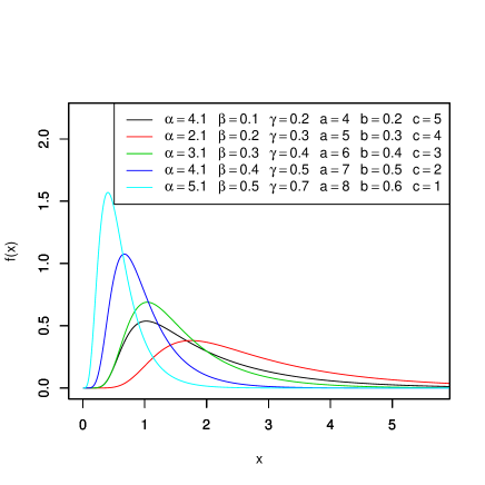
Figure 1. The pdf’s of various McMW distributions.

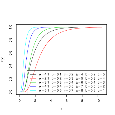
Figure 2. The cdf’s of various McMW distributions.

The hazard function (hf) and reverse hazard functions (rhf) of the Mc-G distribution are given by

(7) $$h(x)=\frac{f(x)}{1-F(x)}=\frac{cg(x)G^{ac-1}(x)\left[1-G^{c}(x)\right]^{b-1}}{B(a,b)\left\{1-I_{G^{c}(x)}(a,b)\right\}},$$

and

$$\tau(x)=\frac{f(x)}{F(x)}=\frac{cg(x)G^{ac-1}(x)\left[1-G^{c}(x)\right]^{b-1}}{B(a,b)\left\{I_{G^{c}(x)}(a,b)\right\}}$$

respectively.

Figure 3 and 4 illustrates some of the possible shapes of the hazard rate function and survival function of McMW distribution for selected values of the parameters $\alpha,\beta.\gamma,a,b$ and $c$.

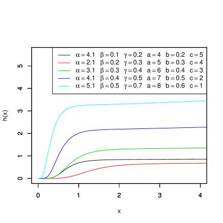
Figure 3. The hazard function of various McMW distributions.

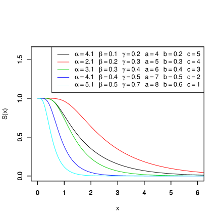
Figure 4. The survival function of various McMW distributions.

Recently Cordeiro et al. (2012) introduced the The McDonald Normal Distribution. Also, Francisco et al. (2012) proposed a new distribution, called the McDonald gamma distribution.

The rest of the paper is organized as follows. In Section 2, we demonstrate that the $McMW$ density function can be expressed as a linear combination of the modified Weibull distribution. This result is important to provide mathematical properties of the $McMW$ model directly from those properties of the modified Weibull distribution in Section 3. In Section 4 we discuss some important statistical properties of the $McMW$ distribution including quantile function, moments , moment generating function. The distribution of the order statistics is expressed in Section 5 . Maximum likelihood estimates of the parameters index to the distribution are discussed in Section 6. Section 7 provides applications to real data sets. Section 8 ends with some conclusions.

2. McDonald Modified Weibull Distribution

In this section we studied the McDonald modified Weibull $(McMW)$ distribution and the sub-models of this distribution. Using $G(x)$ and $g(x)$ in (4)) to be the cdf and pdf of (1) and (2). The pdf of the $McMW$ distribution is given by

$$f(x,\varphi) =\frac{c}{B(a,b)}\left(\alpha+\gamma\beta x^{\beta-1}\right)e^{-\alpha x-\gamma x^{\beta}}\left[1-e^{-\alpha x-\gamma x^{\beta}}\right]^{ac-1}$$

(8) $$\cdot\left[1-\left(1-e^{-\alpha x-\gamma x^{\beta}}\right)^{c}\right]^{b-1},x>0.$$

where $\varphi=(\alpha,\gamma,\beta,a,b,c)$. The corresponding cdf of the $McMW$ distribution is given by

$$F(x) =I_{G^{c}(x)}(a,b)=\frac{1}{B(a,b)}\int\limits_{0}^{G(x)^{c}}w^{(1-a)}(1-w)^{b-1}dw$$

$$=\frac{1}{B(a,b)}\int\limits_{0}^{\left(1-e^{-\alpha x-\gamma x^{\beta}}\right)^{c}}w^{(1-a)}(1-w)^{b-1}dw$$

(9) $$=I_{\left(1-e^{-\alpha x-\gamma x^{\beta}}\right)^{c}}(a,b),$$

also, the cdf can be written as follows

(10) $$F(x)=\frac{\left(1-e^{-\alpha x-\gamma x^{\beta}}\right)^{ac}}{aB(a,b)}\text{ }_{2}F_{1}(a,1-b;a+1;\left[1-e^{-\alpha x-\gamma x^{\beta}}\right]^{c},$$

where ${}_{2}F_{1}(a,b;c;x)=B(b,c-b)^{-1}\int\limits_{0}^{1}\frac{t^{b-1}\left(1-t\right)^{c-b-1}}{\left(1-tx\right)^{a}}dt.$

The hazard rate function and reversed hazard rate function of the new distribution are given by

$$h(x) =\frac{f(x)}{1-F(x)}$$

(11) $$=\frac{c\left(\alpha+\gamma\beta x^{\beta-1}\right)e^{-\alpha x-\gamma x^{\beta}}\left[1-e^{-\alpha x-\gamma x^{\beta}}\right]^{ac-1}\left[1-\left(1-e^{-\alpha x-\gamma x^{\beta}}\right)^{c}\right]^{b-1}}{B(a,b)\left\{1-I_{\left(1-e^{-\alpha x-\gamma x^{\beta}}\right)^{c}}(a,b)\right\}},$$

and

$$\tau(x) =\frac{f(x)}{F(x)}$$

(12) $$=\frac{c\left(\alpha+\gamma\beta x^{\beta-1}\right)e^{-\alpha x-\gamma x^{\beta}}\left[1-e^{-\alpha x-\gamma x^{\beta}}\right]^{ac-1}\left[1-\left(1-e^{-\alpha x-\gamma x^{\beta}}\right)^{c}\right]^{b-1}}{B(a,b)\left\{I_{\left(1-e^{-\alpha x-\gamma x^{\beta}}\right)^{c}}(a,b)\right\}},$$

respectively.

2.1. Submodels

The McDonald modified Weibull distribution is very flexible model that approaches to different distributions when its parameters are changed. The $McMW$ distribution contains as special- models the following well known distributions. If $X$ is a random variable with pdf (2) or cdf (2) we use the notation $X\sim McMW$ $(\alpha,\gamma,\beta,a,b,c)$ then we have the following cases.

1. For $c=1$ , then (2) reduces to the beta modified Weibull $(BMW)$ distribution.

2. For $a=1$ we get the kumaraswamy modified weibull $(KMW)$ distribution.

3. For $\alpha=1$ , then (2) becomes McDonald Weibull $(McW)$ distribution.

4. For $\beta=2$ , we get the McDonald Linear Failure Rate $(McLFR)$ distribution.

5. For $\alpha=0$ and $\beta=2$ , then (2) becomes McDonald Rayleigh $(McR)$ distribution.

6. The McDonald Exponential $(McE)$ distribution arises as a special case of $McMW$ by taking $\gamma=0.$

7. For $\alpha=0$ , $\beta=2$ and $c=1$, then (2) becomes beta Rayleigh $(BR)$ distribution.

8. For $\beta=2$ and $c=1$ , we get the beta Linear Failure Rate $(BLFR)$ distribution.

9. Applying $a=b=c=1$ we can obtain the modified Weibull distribution.

The flexibility of the McDonald modified Weibull distribution is explained in Table (1). The subject distribution includes as special cases the McDonald modified Weibull($McMW$), beta modified Weibull (BMW), Kumaraswamy modified Weibull (KMW), McDonald, McDonald exponential (McE), McDonald linear failure rate (McLFR), modified Weibull (MW), Rayleigh (R), Exponential and Linear failure rate distributions.

Table 1. Sub-models of McMW Distribution.

$Distribution$ $(McMW)$	$\alpha$	$\gamma$	$\beta$	$a$	$b$	$c$
$BMW$	$\alpha$	$\gamma$	$\beta$	$a$	$b$	$1$
$KMW$	$\alpha$	$\gamma$	$\beta$	$1$	$b$	$1$
$McW$	$0$	$\gamma$	$\beta$	$a$	$b$	$c$
$McLFR$	$\alpha$	$\gamma$	$2$	$a$	$b$	$c$
$McR$	$0$	$\gamma$	$2$	$a$	$b$	$c$
$McE$	$\alpha$	$0$	$0$	$a$	$b$	$c$
$BR$	$0$	$\gamma$	$2$	$a$	$b$	$1$
$BLFR$	$\alpha$	$\gamma$	$2$	$a$	$b$	$1$
$MW$	$\alpha$	$\gamma$	$\beta$	$1$	$1$	$1$

3. Expansion of Distribution

In this section,we present a series expansion of the $McMW$  cdf and pdf. distribution depending if the parameter $b>0$ is real non- integer or integer. First, if $\left|z\right|<1$ and $b>0$ is real non- integer, we have

(13) $$(1-z)^{b-1}=\sum\limits_{j=0}^{\infty}(-1)^{j}\binom{b-1}{j}z^{j}=\sum\limits_{j=0}^{\infty}\frac{(-1)^{j}\Gamma(b)}{j!\Gamma(b-j)}z^{j}.$$

Using the expansion (13) in (2), the cdf of the $McMW$ distribution becomes

$$F(x) =\frac{1}{B(a,b)}\int\limits_{0}^{\left(1-e^{-\alpha x-\gamma x^{\beta}}\right)^{c}}w^{(1-a)}(1-w)^{b-1}dw$$

$$=\frac{\Gamma(b)}{B(a,b)}\sum\limits_{j=0}^{\infty}\frac{(-1)^{j}}{j!\Gamma(b-j)}\int\limits_{0}^{G(x)^{c}}w^{a+j-1}dw$$

$$=\sum\limits_{j=0}^{\infty}\frac{(-1)^{j}\Gamma(b)}{B(a,b)j!\Gamma(b-j)(a+j)}\left[G(x,\alpha,\gamma,\beta)\right]^{c(a+j)}$$

$$=\sum\limits_{j=0}^{\infty}q_{j}\text{ }G(x,\alpha c(a+j),\gamma,\beta)$$

If $b>0$ is an integer, then

(14) $$F(x)=\sum\limits_{j=0}^{b-1}q_{j}G(x,\alpha c(a+j),\gamma,\beta).$$

Similarly, if $b>0$ is real non- integer the pdf is given by

(15) $$f(x)=\sum\limits_{j=0}^{\infty}q_{j}g(x,\alpha c(a+j),\gamma,\beta),$$

and

(16) $$f(x)=\sum\limits_{j=0}^{b-1}q_{j}g(x,\alpha c(a+j),\gamma,\beta),$$

for $b>0$ is an integer. Where $q_{j}=\frac{(-1)^{j}\Gamma(b)}{B(a,b)j!\Gamma(b-j)(a+j)}$ are constants such that $\sum\limits_{j=0}^{\infty}q_{j}=1$ and $G(x,\alpha c(a+j),\gamma,\beta)$ is a finite mixture of modified Weibull distribution with scale parameter $\alpha c(a+j)$ and $\gamma,\beta$ are shape parameters.

4. Statistical Properties

In this section we discuss the statistical properties of the McDonald modified Weibull distribution, in particular, quantile function, moment and moment generating function.

4.1. Quantile function

The $McQL$ quantile function , say $Q(u)=F^{-1}(u)$, is straightforward to be computed by inverting (LABEL:eq1.8), we have

(17) $$\gamma x_{q}^{\beta}+\alpha x_{q}^{\theta}+\ln\left[1-Q_{(a,b)}(u)^{\frac{1}{c}})\right]=0,$$

we can easily generate $X$ by taking $u$ as a uniform random variable in $(0,1)$.

4.2. Moments

In this subsection we discuss the $r_{th}$ moment for $McMW$ distribution. Moments are necessary and important in any statistical analysis, especially in applications. It can be used to study the most important features and characteristics of a distribution (e.g., tendency, dispersion, skewness and kurtosis).

Theorem (4.1). If $X$ has $McMW$ $(\varphi,x)$ $,\varphi=(\alpha,\gamma,\beta,a,b,c)$ then the $k_{th}$ moment of $X$ is given by the following

(18) $$\mu_{r}(x)=w_{j,m,s}\left[\frac{\alpha\Gamma(k+\beta s+1)}{\left[m(\alpha+1)\right]^{k+\beta s+1}}+\frac{\gamma\beta\Gamma(k+\beta(s+1))}{\left[m(\alpha+1)\right]^{k+\beta(s+1)}}\right].$$

Proof:

Let $X$ be a random variable with density function (2). The $k_{th}$ ordinary moment of the $McMW$ distribution is given by

$$\mu_{k}^{{}^{\prime}}(x) =E(X^{k)}=\int\limits_{0}^{\infty}x^{k}f(x,\varphi)dx$$

(19) $$=\frac{c}{B(a,b)}\int\limits_{0}^{\infty}x^{k}\left(\alpha+\gamma\beta x^{\beta-1}\right)e^{-\alpha x-\gamma x^{\beta}}\left[1-e^{-\alpha x-\gamma x^{\beta}}\right]^{ac-1}\left[1-\left(1-e^{-\alpha x-\gamma x^{\beta}}\right)^{c}\right]^{b-1}dx.$$

Setting

(20) $$\left[1-\left(1-e^{-\alpha x-\gamma x^{\beta}}\right)^{c}\right]^{b-1}=\sum\limits_{j=0}^{\infty}(-1)^{j}\binom{b-1}{j}\left(1-e^{-\alpha x-\gamma x^{\beta}}\right)^{cj},$$

so

$$\mu_{k}^{{}^{\prime}}(x)=\frac{c}{B(a,b)}\sum\limits_{j=0}^{\infty}(-1)^{j}\binom{b-1}{j}\int\limits_{0}^{\infty}x^{k}\left(\alpha+\gamma\beta x^{\beta-1}\right)e^{-\alpha x-\gamma x^{\beta}}\left[1-e^{-\alpha x-\gamma x^{\beta}}\right]^{c(a+j)-1}$$

but

(21) $$\left[1-e^{-\alpha x-\gamma x^{\beta}}\right]^{c(a+j)-1}=\sum\limits_{k=0}^{\infty}(-1)^{m}\binom{c(j+a)-1}{m}e^{-m\alpha x-m\gamma x^{\beta}},$$

then

$$\mu_{k}^{{}^{\prime}}(x) =\frac{c}{B(a,b)}\sum\limits_{j=0}^{\infty}\sum\limits_{m=0}^{\infty}(-1)^{j+m}\binom{b-1}{j}\binom{c(j+a)-1}{m}$$

(22) $$\times\int\limits_{0}^{\infty}x^{k}\left(\alpha+\gamma\beta x^{\beta-1}\right)e^{-m(\alpha+1)x-m(\gamma+1)x^{\beta}}dx$$

using the following expansion of $e^{-m(\gamma+1)x^{\beta}}$ given by

$$e^{-m(\gamma+1)x^{\beta}}=\sum\limits_{s=0}^{\infty}\frac{(-1)^{s}}{s!}\left[m(\gamma+1)\right]^{s}x^{\beta s}$$

thus equation (4.2) takes the following form

$$\mu_{k}^{{}^{\prime}}(x) =\frac{c\left[m(\gamma+1)\right]^{s}}{B(a,b)s!}\sum\limits_{j,m,s=0}^{\infty}(-1)^{j+m+s}\binom{b-1}{j}\binom{c(j+a)-1}{m}$$

$$\times\left\{\alpha\int\limits_{0}^{\infty}x^{k+\beta s}e^{-m(\alpha+1)x}dx+\gamma\beta\int\limits_{0}^{\infty}x^{k+\beta(s+1)-1}e^{-m(\alpha+1)x}dx\right\}$$

(23) $$=w_{j,m,s}\left[\frac{\alpha\Gamma(k+\beta s+1)}{\left[m(\alpha+1)\right]^{k+\beta s+1}}+\frac{\gamma\beta\Gamma(k+\beta(s+1))}{\left[m(\alpha+1)\right]^{k+\beta(s+1)}}\right]$$

where

$$w_{j,m,s}=\frac{c\left[m(\gamma+1)\right]^{s}}{B(a,b)s!}\sum\limits_{j,m,s=0}^{\infty}(-1)^{j+m+s}\binom{b-1}{j}\binom{c(j+a)-1}{m}.$$

Which completes the proof .
Based on the first four moments of the $(McMW)$ distribution, the measures of skewness $A(\varphi)$ and kurtosis $k(\varphi)$ of the $(McMW)$ distribution can obtained as

(24) $$A(\varphi)=\frac{\mu_{3}(\theta)-3\mu_{1}(\theta)\mu_{2}(\theta)+2\mu_{1}^{3}(\theta)}{\left[\mu_{2}(\theta)-\mu_{1}^{2}(\theta)\right]^{\frac{3}{2}}},$$

and

(25) $$k(\varphi)=\frac{\mu_{4}(\theta)-4\mu_{1}(\theta)\mu_{3}(\theta)+6\mu_{1}^{2}(\theta)\mu_{2}(\theta)-3\mu_{1}^{4}(\theta)}{\left[\mu_{2}(\theta)-\mu_{1}^{2}(\theta)\right]^{2}}.$$

Theorem (4.2):

If $X$ has the $McMW$ $(\alpha,\gamma,\beta,a,b,c,x)$ then the the moment generating function (mgf) of $X$  is given as follows

(26) $$M_{X}(t)=w_{j,m,s}\left[\frac{\alpha\Gamma(\beta s+1)}{\left[m(\alpha+1)-t\right]^{\beta s+1}}+\frac{\gamma\beta\Gamma(\beta(s+1))}{\left[m(\alpha+1)-t\right]^{\beta(s+1)}}\right].$$

Proof:

Starting with

$$M_{X}(t) =\int\limits_{0}^{\infty}e^{tx}f_{McMW}(\alpha,\gamma,\beta,a,b,c,x)dx$$

$$=w_{j,m,s}\int\limits_{0}^{\infty}(\alpha x^{\beta s}+\gamma\beta x^{\beta(s+1)-1})e^{-x(m(\alpha+1)-t)}dx$$

$$=w_{j,m,s}\left\{\alpha\int\limits_{0}^{\infty}x^{\beta s}e^{-x(m(\alpha+1)-t)}dx+\gamma\beta\int\limits_{0}^{\infty}x^{\beta(s+1)-1}e^{-x(m(\alpha+1)-t)}dx\right\}$$

(27) $$=w_{j,m,s}\left[\frac{\alpha\Gamma(\beta s+1)}{\left[m(\alpha+1)-t\right]^{\beta s+1}}+\frac{\gamma\beta\Gamma(\beta(s+1))}{\left[m(\alpha+1)-t\right]^{\beta(s+1)}}\right]$$

Which completes the proof.

5. Distribution of the order statistics

In this section, we derive closed form expressions for the pdfs of the $r_{th}$ order statistic of the $(McMW)$ distribution, also, the measures of skewness and kurtosis of the distribution of the $r_{th}$ order statistic in a sample of size $n$ for different choices of $n;r$ are presented in this section. Let $X_{1},X_{2},...,X_{n}$ be a simple random sample from $(McMW)$ distribution with pdf and cdf given by (2) and (10), respectively.

Let $X_{1},X_{2},...,X_{n}$ denote the order statistics obtained from this sample. We now give the probability density function of $X_{r:n}$, say $f_{r:n}(x,\varphi)$ and the moments of $X_{r:n}$ $,r=1,2,...,n$. Therefore, the measures of skewness and kurtosis of the distribution of the $X_{r:n}$ are presented. The probability density function of $X_{r:n}$ is given by

(28) $$f_{r:n}(x,\varphi)=\frac{1}{B(r,n-r+1)}\left[F(x,\Phi)\right]^{r-1}\left[1-F(x,\Phi)\right]^{n-r}f(x,\varphi)$$

where $F(x,\varphi)$ and $f(x,\varphi)$ are the cdf and pdf of the $(McMW)$ distribution given by (2), (10), respectively, and $B$ $(.,.)$ is the beta function, since $0<F(x,\varphi)<1$, for $x>0$, by using the binomial series expansion of $\left[1-F(x,\varphi)\right]^{n-r}$, given by

(29) $$\left[1-F(x,\varphi)\right]^{n-r}=\sum\limits_{j=0}^{n-r}(-1)^{j}\binom{n-r}{j}\left[F(x,\varphi)\right]^{{}^{j}},$$

we have

(30) $$f_{r:n}(x,\varphi)=\sum\limits_{j=0}^{n-r}(-1)^{j}\binom{n-r}{j}\left[F(x,\Phi)\right]^{r+j-1}f(x,\varphi),$$

substituting from (2) and (10) into (30)), we can express the $k_{th}$ ordinary moment of the $r_{th}$ order statistics $X_{r:n}$ say $E(X_{r:n}^{k})$ as a liner combination of the $k_{th}$ moments of the $(McMW)$ distribution with different shape parameters. Therefore, the measures of skewness and kurtosis of the distribution of $X_{r:n}$ can be calculated.

6. Maximum Likelihood Estimators

In this section we consider the maximum likelihood estimators (MLE’s) of $McMW$ $(\alpha,\gamma,\beta,a,b,c,x)$ . Let $x_{1},...,$ $x_{n}$ be a random sample of size $n$ from $McMW$ $(\alpha,\gamma,\beta,a,b,c,x)$ then the likelihood function can be written as$e^{-\alpha x-\gamma x^{\beta}}$

$$L(\alpha,\beta,\theta,\gamma,\lambda,x_{{}_{(i)}}) =\prod\limits_{i=1}^{n}\left(\frac{c}{B(a,b)}\right)\prod\limits_{i=1}^{n}\left(\alpha+\gamma\beta x_{i}^{\beta-1}\right)\prod\limits_{i=1}^{n}e^{-\alpha\sum\limits_{i=1}^{n}x_{i}-\gamma\sum\limits_{i=1}^{n}x_{i}^{\beta}}$$

(31) $$cdot\prod\limits_{i=1}^{n}\left[1-e^{-\alpha x_{i}-\gamma x_{i}^{\beta}}\right]^{ac-1}\prod\limits_{i=0}^{n}\left[1-\left(1-e^{-\alpha x_{i}-\gamma x_{i}^{\beta}}\right)^{c}\right]^{b-1}$$

By accumulation taking logarithm of equation (6) , and the log- likelihood function can be written as

$$\ell=\log L =n\log c+n\log\left[\Gamma(a+b)\right]-n\log\left[\Gamma(a)\right]-n\log\left[\Gamma(b)\right]$$

$$+\sum\limits_{i=1}^{n}\log\left(\alpha+\gamma\beta x_{i}^{\beta-1}\right)-\alpha\sum\limits_{i=1}^{n}x_{i}-\gamma\sum\limits_{i=1}^{n}x_{i}^{\beta}$$

$$+(ac-1)\sum\limits_{i=1}^{n}\log\left[1-e^{-\alpha x_{i}-\gamma x_{i}^{\beta}}\right]$$

(32) $$+(b-1)\sum\limits_{i=1}^{n}\log\left[1-\left(1-e^{-\alpha x_{i}-\gamma x_{i}^{\beta}}\right)^{c}\right].$$

Computing the first partial derivatives of $\ell$ and setting the results equal zeros, we get the likelihood equations as in the following form

(33) $$\frac{\partial\ell}{\partial a}=n\psi(a+b)-n\psi(a)+c\sum\limits_{i=1}^{n}\log\left[1-e^{-\alpha x_{i}-\gamma x_{i}^{\beta}}\right],$$

(34) $$\frac{\partial\ell}{\partial b}=n\psi(a+b)-n\psi(b)+\sum\limits_{i=1}^{n}\log\left[1-\left(1-e^{-\alpha x_{i}-\gamma x_{i}^{\beta}}\right)^{c}\right],$$

$$\frac{\partial\ell}{\partial c} =\frac{n}{c}+a\sum\limits_{i=1}^{n}\log\left[1-e^{-\alpha x_{i}-\gamma x_{i}^{\beta}}\right]$$

(35) $$-(b-1)\sum\limits_{i=1}^{n}\frac{\left(1-e^{-\alpha x_{i}-\gamma x_{i}^{\beta}}\right)^{c}\log\left(1-e^{-\alpha x_{i}-\gamma x_{i}^{\beta}}\right)}{\left[1-\left(1-e^{-\alpha x_{i}-\gamma x_{i}^{\beta}}\right)^{c}\right]},$$

$$\frac{\partial\ell}{\partial\alpha} =\sum\limits_{i=1}^{n}\frac{1}{\left(\alpha+\gamma\beta x_{i}^{\beta-1}\right)}-\sum\limits_{i=1}^{n}x_{i}+(ac-1)\sum\limits_{i=1}^{n}\frac{x_{i}e^{-\alpha x_{i}-\gamma x_{i}^{\beta}}}{\left[1-e^{-\alpha x_{i}-\gamma x_{i}^{\beta}}\right]}$$

(36) $$+c(b-1)\sum\limits_{i=1}^{n}\frac{x_{i}e^{-\alpha x_{i}-\gamma x_{i}^{\beta}}\left(1-e^{-\alpha x_{i}-\gamma x_{i}^{\beta}}\right)^{c-1}}{\left[1-\left(1-e^{-\alpha x_{i}-\gamma x_{i}^{\beta}}\right)^{c}\right]},$$

$$\frac{\partial\ell}{\partial\gamma} =\sum\limits_{i=1}^{n}\frac{\beta x_{i}^{\beta-1}}{\left(\alpha+\gamma\beta x_{i}^{\beta-1}\right)}-\sum\limits_{i=1}^{n}x_{i}^{\beta}+(ac-1)\sum\limits_{i=1}^{n}\frac{x_{i}^{\beta}e^{-\alpha x_{i}-\gamma x_{i}^{\beta}}}{\left[1-e^{-\alpha x_{i}-\gamma x_{i}^{\beta}}\right]}$$

(37) $$+(b-1)\sum\limits_{i=1}^{n}\frac{x_{i}^{\beta}e^{-\alpha x_{i}-\gamma x_{i}^{\beta}}\left(1-e^{-\alpha x_{i}-\gamma x_{i}^{\beta}}\right)^{c-1}}{\left[1-\left(1-e^{-\alpha x_{i}-\gamma x_{i}^{\beta}}\right)^{c}\right]},$$

and

$$\frac{\partial\ell}{\partial\beta} =\sum\limits_{i=1}^{n}\frac{\gamma x_{i}^{\beta-1}\left(\beta\log x_{i}+1\right)}{\left(\alpha+\gamma\beta x_{i}^{\beta-1}\right)}-\gamma\sum\limits_{i=1}^{n}x_{i}^{\beta}\log x_{i}$$

$$+\gamma(ac-1)\sum\limits_{i=1}^{n}\frac{x_{i}^{\beta}\log x_{i}e^{-\alpha x_{i}-\gamma x_{i}^{\beta}}}{\left[1-e^{-\alpha x_{i}-\gamma x_{i}^{\beta}}\right]}$$

(38) $$+\gamma c(b-1)\sum\limits_{i=1}^{n}\frac{x_{i}^{\beta}\log x_{i}e^{-\alpha x_{i}-\gamma x_{i}^{\beta}}\left(1-e^{-\alpha x_{i}-\gamma x_{i}^{\beta}}\right)^{c-1}}{\left[1-\left(1-e^{-\alpha x_{i}-\gamma x_{i}^{\beta}}\right)^{c}\right]}.$$

By solving this nonlinear system of equations (33) - (6), these solutions will yield the ML estimators for $\widehat{a}$,$\widehat{b}$ , $\widehat{c}$ $,\widehat{\alpha}$, $\widehat{\beta}$ and $\widehat{\gamma}$ , for the six parameters McDonald modified Weibull distribution $McMW$ $(\alpha,\gamma,\beta,a,b,c,x)$ pdf all the second order derivatives exist. Thus we have the inverse dispersion matrix is given by

(39) $$\left(\begin{array}[]{c}\widehat{\alpha}\\ \widehat{\theta}\\ \widehat{\beta}\\ \widehat{a}\\ \widehat{b}\\ \widehat{c}\end{array}\right)\sim N\left[\left(\begin{array}[]{c}\alpha\\ \theta\\ \beta\\ a\\ b\\ c\end{array}\right),\left(\begin{array}[]{cccccc}\widehat{V_{\alpha\alpha}}&\widehat{V_{\alpha\theta}}&\widehat{V_{\alpha\beta}}&\widehat{V_{\alpha a}}&\widehat{V_{\alpha b}}&\widehat{V_{\alpha c}}\\ \widehat{V_{\theta\alpha}}&\widehat{V_{\theta\theta}}&\widehat{V_{\theta\beta}}&\widehat{V_{\theta a}}&\widehat{V_{\theta b}}&\widehat{V_{\theta c}}\\ \widehat{V_{\beta\alpha}}&\widehat{V_{\beta\theta}}&\widehat{V_{\beta\beta}}&\widehat{V_{\beta a}}&\widehat{V_{\beta b}}&\widehat{V_{\beta c}}\\ \widehat{V_{a\alpha}}&\widehat{V_{a\theta}}&\widehat{V_{a\beta}}&\widehat{V_{aa}}&\widehat{V_{ab}}&\widehat{V_{ac}}\\ \widehat{V_{b\alpha}}&\widehat{V_{b\theta}}&\widehat{V_{b\beta}}&\widehat{V_{ba}}&\widehat{V_{bb}}&\widehat{V_{bc}}\\ \widehat{V_{c\alpha}}&\widehat{V_{c\theta}}&\widehat{V_{c\beta}}&\widehat{V_{ca}}&\widehat{V_{cb}}&\widehat{V_{cc}}\end{array}\right)\right].$$

(40) $$V^{-1}=-E\left[\begin{array}[]{cccccc}V_{\alpha\alpha}&V_{\alpha\theta}&V_{\alpha\beta}&V_{\alpha a}&V_{\alpha b}&V_{\alpha c}\\ &&&&&\\ &&&&&\\ &&&&&\\ &&&&&\\ V_{c\alpha}&V_{c\theta}&V_{c\beta}&V_{ca}&V_{cb}&V_{cc}\end{array}\right]$$

where

$$V_{\alpha\alpha} =\frac{\partial^{2}L}{\partial\alpha^{2}},V_{\gamma\gamma}=\frac{\partial^{2}L}{\partial\gamma^{2}},V_{\beta\beta}=\frac{\partial^{2}L}{\partial\beta^{2}}$$

$$V_{aa} =\frac{\partial^{2}L}{\partial a^{2}},V_{bb}=\frac{\partial^{2}L}{\partial b^{2}},V_{cc}=\frac{\partial^{2}L}{\partial c^{2}}$$

$$V_{a\alpha} = \frac{\partial^{2}L}{\partial\alpha\partial a},V_{{}_{\theta\beta}}=\frac{\partial^{2}L}{\partial\theta\partial\beta},V_{\beta\gamma}=\frac{\partial^{2}L}{\partial\beta\partial\gamma}$$

By solving this inverse dispersion matrix these solutions will yield asymptotic variance and covariances of these ML estimators for $\widehat{a}$,$\widehat{b}$ , $\widehat{c}$ $,\widehat{\alpha}$, $\widehat{\beta}$ and $\widehat{\gamma}$ . Using (39), we approximate $100(1-\gamma)\%$ confidence intervals for $a,b,c,\alpha,\beta,$and $\gamma,$are determined respectively as

$$\widehat{\alpha}\pm z_{\frac{\gamma}{2}}\sqrt{\widehat{V_{\alpha\alpha}}},\text{ }\widehat{a}\pm z_{\frac{\gamma}{2}}\sqrt{\widehat{V_{aa}}}\text{\ , }\widehat{\beta}\pm z_{\frac{\gamma}{2}}\sqrt{\widehat{V_{\beta\beta}}}$$

$$\widehat{\gamma}\pm z_{\frac{\gamma}{2}}\sqrt{V_{\gamma\gamma}},\widehat{b}\pm z_{\frac{\gamma}{2}}\sqrt{\widehat{V_{bb}}}\text{ and }\widehat{c}\pm z_{\frac{\gamma}{2}}\sqrt{\widehat{Vcc}}$$

where $z_{\gamma}$ is the upper $100\gamma_{the}$ percentile of the standard normal distribution.

7. Application

In this section, we use a real data set to show that the McMW distribution can be a better model than one based on the MW distribution and Weibull distribution. The data set given in Table 1 taken from [12] page 180 represents the failure times of 50 components(per 1000h):

Table 2. Failure Times of 50 Components(per 1000 hours).

0.036	0.058	0.061	0.074	0.078	0.086	0.102	0.103	0.114	0.116
0.148	0.183	0.192	0.254	0.262	0.379	0.381	0.538	0.570	0.574
0.590	0.618	0.645	0.961	1.228	1.600	2.006	2.054	2.804	3.058
3.076	3.147	3.625	3.704	3.931	4.073	4.393	4.534	4.893	6.274
6.816	7.896	7.904	8.022	9.337	10.940	11.020	13.880	14.730	15.080

Table 3. Estimated parameters of the Modified Weibull and McMW distribution for the failure times of 50 components(per 1000h).

Model	Parameter Estimate	Standard Error	$-\ell(\cdot;x)$
Modified	$\hat{\alpha}=0.043$	$0.131$	102.320
Weibull	$\hat{\beta}=0.492$	0.181
	$\hat{\gamma}=0.619$	0.154
Mc Donald	$\hat{\alpha}=0.599$	1.116e-05	98.404
modified	$\hat{\beta}=1.063$	0.012
Weibull	$\hat{\gamma}=1.209$	0.003
	$\hat{a}=0.091$	0.015
	$\hat{b}=0.090$	0.015
	$\hat{c}=9.169$	0.018

The variance covariance matrix $I(\hat{\varphi})^{-1}$ of the MLEs under the McMW distribution is computed as

$$\begin{pmatrix}1.2\cdot 10^{-4}&-1.3\cdot 10^{-4}&6.2\cdot 10^{-6}&7.0\cdot 10^{-6}&1.2\cdot 10^{-5}&8.6\cdot 10^{-4}\\ -1.3\cdot 10^{-4}&1.4\cdot 10^{-4}&-1.1\cdot 10^{-5}&-7.6\cdot 10^{-6}&-1.2\cdot 10^{-5}&-9.3\cdot 10^{-4}\\ 6.2\cdot 10^{-6}&-1.1\cdot 10^{-5}&9.5\cdot 10^{-6}&6.0\cdot 10^{-7}&7.2\cdot 10^{-7}&6.4\cdot 10^{-5}\\ 7.0\cdot 10^{-6}&-7.6\cdot 10^{-6}&6.0\cdot 10^{-7}&2.4\cdot 10^{-4}&8.6\cdot 10^{-5}&6.5\cdot 10^{-5}\\ 1.2\cdot 10^{-5}&-1.2\cdot 10^{-5}&7.2\cdot 10^{-7}&8.6\cdot 10^{-5}&2.4\cdot 10^{-4}&8.4\cdot 10^{-5}\\ 8.6\cdot 10^{-4}&-9.3\cdot 10^{-4}&6.4\cdot 10^{-5}&6.5\cdot 10^{-5}&8.4\cdot 10^{-5}&3.5\cdot 10^{-3}\\ \end{pmatrix}\,.$$

Thus, the variances of the MLE of $\alpha,\beta,\gamma,a,b$ and $c$ is $var(\hat{\alpha})=1.247\cdot 10^{-4},var(\hat{\beta})=1.488\cdot 10^{-4},$ $var(\hat{\gamma})=9.529\cdot 10^{-6},var(\hat{a})=2.472\cdot 10^{-4},$ $var(\hat{b})=2.467\cdot 10^{-4},var(\hat{c})=3.544\cdot 10^{-3}.$

Therefore, $95\%$ confidence intervals for $\alpha,\beta,\gamma,a,b$ and $c$ are $[0.599,0.601],[1.039,1.086],[1.202,1.215],[0.06,0.121],[0.059,0.121]$ and $[9.132,9.205]$ respectively.

Table 4. Criteria for comparison.

Model K-S	$-2\ell$	AIC	AICC
MW 0.128	204.640	210.64	211.161
McMW 0.118	196.808	208.808	210.761

In order to compare the two distribution models, we consider criteria like , $-2\ell$, AIC (Akaike information criterion)and AICC (corrected Akaike information criterion) for the data set. The better distribution corresponds to smaller $-2\ell$, AIC and AICC values:‘

$$\mbox{AIC}=2k-2\ell\,,\quad\textrm{and}\mbox{AICC}=\mbox{AIC}+\frac{2k(k+1)}{n-k-1}\,,$$

where $k$ is the number of parameters in the statistical model, $n$ the sample size and $\ell$ is the maximized value of the log-likelihood function under the considered model. Table 3 shows the MLEs under both distributions, table 4 shows the values of K-S, $-2\ell$, AIC and AICC values. The values in table 3 indicate that the McMW distribution leads to a better fit than the MW distribution and Weibull distribution.

A density plot compares the fitted densities of the models with the empirical histogram of the observed data (Fig. 4). The fitted density for the McMW model is closer to the empirical histogram than the fits of the MW and Weibull sub-models.

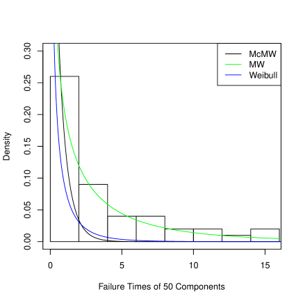
Figure 5. Estimated densities of the models for the failure times of 50 components.

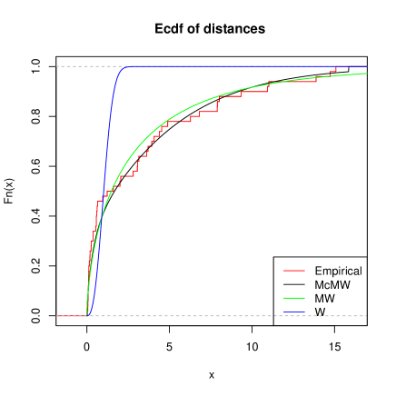
Figure 6. Empirical, fitted Weibull, MW and McMW cdf of the failure times of 50 components.

8. Conclusion

Here we propose a new model, the so-called the Mc Donald Modified Weibull distribution which extends the modified Weibull distribution in the analysis of data with real support. An obvious reason for generalizing a standard distribution is because the generalized form provides larger flexibility in modeling real data. We derive expansions for moments and for the moment generating function. The estimation of parameters is approached by the method of maximum likelihood, also the information matrix is derived. An application of McMW distribution to real data show that the new distribution can be used quite effectively to provide better fits than modified Weibull and Weibull distribution.

References

• [1] Aarset, M. V. (1987). How to identify a bathtub hazard rate. Reliability, IEEE Transactions on, 36(1), 106-108.
• [2] Bain, L. J. (1974). Analysis for the linear failure-rate life-testing distribution. Technometrics, 16(4), 551-559.
• [3] Barlow R. E., and Proschan F. (1981). Statistical Theory of Reliability and Life Testing, Begin With, Silver Spring, MD,.
• [4] Carrasco, J. M., Ortega, E. M., and Cordeiro, G. M. (2008). A generalized modified Weibull distribution for lifetime modeling. Computational Statistics and Data Analysis, 53(2), 450-462.
• [5] Eddy, O. N. (2007). Applied statistics in designing special organic mixtures. Applied Sciences, 9, 78-85.
• [6] Gradshteyn, I. S., and Ryzhik, I. M. (2000). Table of Integrals, Series, and Products 6th edn (New York: Academic).
• [7] Ghitany, M. E., and Kotz, S. (2007). Reliability properties of extended linear failure-rate distributions. Probability in the Engineering and informational Sciences, 21(3), 441.
• [8] Lawless J. F. (2003). Statistical Models and Methods for Lifetime Data, John Wiley and Sons, New York.
• [9] Lee, C., Famoye, F., and Olumolade, O. (2007). Beta-Weibull distribution: some properties and applications to censored data. Journal of modern applied statistical methods, 6(1), 17.
• [10] Lin, C. T., Wu, S. J., and Balakrishnan, N. (2006). Monte Carlo methods for Bayesian inference on the linear hazard rate distribution. Communications in Statistics—Simulation and Computation, 35(3), 575-590.
• [11] Miller Jr, R. G. (2011). Survival analysis (Vol. 66). John Wiley and Sons.
• [12] Murthy, D. P., Xie, M., and Jiang, R. (2004). Weibull models (Vol. 505). John Wiley and Sons.
• [13] Silva, G. O., Ortega, E. M., and Cordeiro, G. M. (2010). The beta modified Weibull distribution. Lifetime data analysis, 16(3), 409-430.
• [14] Tadj, L., Sarhan, A. M., and El-Gohary, A. (2008). Optimal control of an inventory system with ameliorating and deteriorating items. Applied Sciences, 10, 243-255.
• [15] Zhang, Z., Sun, H., and Zhong, F. (2007). Information geometry of the power inverse Gaussian distribution. Applied Sciences (APPS), 9, 194-203.