Self-Organization In 1-d Swarm Dynamics

Abstract

Self-organization of a biologically motivated swarm into smaller subgroups of different velocities is found by solving a 1-dimensional adaptive-velocity swarm, in which the velocity of an agent is averaged over a finite local radius of influence. Using a mean field model in phase space, we find a dependence of this group-division phenomenon on the typical scales of the initial swarm in the position and velocity dimensions. Comparisons are made to previous swarm models in which the speed of an agent is either fixed or adjusted according to the degree of direction consensus among its local neighbors.

Key words: self-organization of swarm, phase space, multi-agent system, dynamical system, group-division.

PACS:89.75.Fb, 05.65.+b

1 Introduction

The dynamics of swarm behavior has long been a mystery in nature [12]-[17], and despite intensive work, remains an open problem today [1]-[11]. Examples of swarms include flocks of birds, schools of fishes and even crowds of people in cramped public spaces. This research effort has introduced a wide range of models for swarm behavior which is the background for our model in this paper. In 1986, Reynolds [1] simulated swarm behavior according to the following rules: move in the same direction as the neighbors; remain close to the neighbors; avoid collisions with neighbors. In 1995, Vicsek et al. [2] proposed an important simpler model, in which all the agents have a constant speed and only change their headings according to the other agents in the influence radius (cf. also [3, 4, 7, 8]).

Other models for swarm behavior include [5, 6, 8, 9, 10, 11]. In 1995, Toner and Tu [5] proposed a non-equilibrium continuous dynamical model for the collective motion of large groups of biological organisms. It describes a class of microscopic rules, which includes the model in [2] as a special case. In 2003, Aldana and Huepe [6] investigated the conditions that produce a phase transition from an ordered to a disordered state in a model of two-dimensional agents with a ferromagnetic-like interaction. In their model, the agents still keep a constant speed and change their headings as in [2]. However, they are only influenced by their neighbors in a fixed radius. Besides, Morale et al [9]-[11] have proposed stochastic models for swarms from 2000. These models are based on a number of individuals subject to several distinct mechanisms simultaneously - long range attraction, and short range repulsion, in addition to a classical Brownian random dispersal.

In 2008, Nabet, Benjamin, et al. [7] established a model simpler than [2], in which the agent speed is fixed and the effects of agent position are ignored. The swarm in their model includes two informed subgroups which have preferred directions of motion and a third naive group that does not have a preference. They investigate the tendency for members of the naive group to join the other two groups and the conditions that govern this behavior. This behavior to divide into subgroups is also what we focus on in our paper. However, in our model, the division occurs spontaneously without any special bias in the initial conditions of the swarm.

In 2011, W.Li and X.Wang [8] proposed another model which is also based on [2]. In their model, each agent adjusts its heading and speed simultaneously according to its local neighbors. The change in speed at each time step depends only on the degree of local direction consensus. Unlike our model, the new speed does not depend on the previous speed or the speeds of nearby agents.

Motivated by the aim of a more complete understanding of swarm behavior in the real world, we introduce a new model in 1-dimensional space, in which each agent continuously updates its speed and direction according to the average velocity of the agents within its influence radius. We simulate the model with initial positions and velocities for the agents that are randomly drawn from respective Gaussian distributions, and observe that there is a robust non-equilibrium group-division phenomenon. We eventually determine the time-scale of the group-division by analyzing the rates of energy decrease in the system. It is our aim in this 1-dimensional model to isolate within a simple framework, one swarm mechanism which is velocity-adaptive according to local velocity averages. Despite its simplicity and spatial 1-dimensionality, the robust group-division phenomenon that we found, appears to be related to some aspects of the swarm behavior observed in the natural world [16, 17].

The paper is organized as follows. In section 2, we formulate the discrete and mean field models in this paper. In section 3, we discuss simulations conducted using these models to find the effects of typical scales of initial position and velocity on the group-division phenomenon. Then we examine the energetics of this group-division phenomenon, and calculate the time when division completes in section 4. Conclusions are given in section 5.

2 models

2.1 Discrete model

We consider a swarm of $N$ agents $\{a_{1},a_{2},...,a_{N}\}$ in 1-d space, each of which has velocity $v_{i}$ and position $p_{i}$, and assume that every agent can sense the other agents within the fixed radius $r$. We call these agents its neighbors and assume each agent adjusts its velocity according to the average velocity of the neighbors. For agent $a_{i}$, Let $n_{i}$ be the number of neighbors around it, and $\{a_{i1},a_{i2},...,a_{{in}_{i}}\}$ are corresponding neighbors, let $v_{ij}$ be the velocity of agent $a_{ij}$; according to the assumption, for each i = ${1,...,N}$:

$${dv_{i}\over dt}={1\over n_{i}}\sum_{j=1}^{n_{i}}v_{ij}-v_{i}.$$

We also have:

$${dp_{i}\over dt}=v_{i}.$$

Together, we get the equations in 2 dimensional phase space given by position and velocity.

Simulation of this model in two-dimensional phase space, as shown in Figure.1, reveals a group-division phenomenon in the dynamics. We measure the typical scales of initial position and velocity by the standard deviations ($\sigma(p)$, $\sigma(v)$) in the corresponding dimensions, define ($\sigma(p)$, $\sigma(v)$) as

$$\sigma(p)=\sqrt{{1\over{N-1}}\sum_{j=1}^{N}({p_{j}}-\overline{p})^{2}},$$

and

$$\sigma(v)=\sqrt{{1\over{N-1}}\sum_{j=1}^{N}({v_{j}}-\overline{v})^{2}}.$$

Then we generate the initial swarm using Gaussian distribution with typical scales $\sigma(p)$ and $\sigma(v)$ respectively. We run this model 20000 periods for 1000 agents, in each period, all the agents adjust their velocity in response to their neighbors. At the beginning, there is only one huge group; as the time goes by, the huge group starts to divide into several small groups, each group has its own velocity.

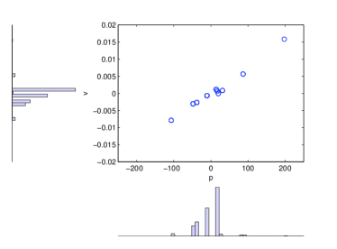
Figure 1: Initial condition: typical scale of $p$: $\sigma(p)=\sqrt{150}$; typical scale of $v$: $\sigma(v)=0.025$; influence radius: $r=0.05$; number of agents: $N=1000$; length of each time step: $dt=0.5$ and totally 20000 period. X-axis and y-axis represent position and velocity respectively. The histograms in the left and under the figure are the projection of the number of agents in the y-axis and the x-axis respectively. At the beginning of the simulation, there is only one group; as the time goes by, the group starts to divide into several small groups with most of the agents near the origin of the phase space.

2.2 Mean field model

We use a mean field method to build a model in phase space. Assume the number of agents in the swarm is large enough; also the agents in any small area in phase space is well-distributed. Let $v,p$ be the velocity and position as before. Define $\rho$ as the probability measure in phase space — for any point $x=(p,v)$ in phase space, $\rho(x)$ is defined as the probability for an agent to be in the neighborhood of $x$:

$$\rho(x)=\lim_{\varepsilon\rightarrow 0}{prob\{a\in B(x,\varepsilon)\}\over\|B(x,\varepsilon)\|},$$

where $B(x,\varepsilon)$ denotes a ball of radius $\varepsilon$ centered at point $x$.

Let $t$ denote the time, $r$ denote the influencing radius. Define $u$ as the flow velocity in phase space, and define $Nb(p)=\{(p^{\prime},v^{\prime})|p^{\prime}\in(p-r,p+r),v^{\prime}\in(-\infty,\infty)\}$. Then

$$\int_{-\infty}^{\infty}(\int_{p_{0}-r}^{p_{0}+r}\rho(p,v)dp)\cdot dv=E[\mbox{number of agents in}\ Nb(p)],$$

where $E[\ ]$ denotes the expectation. Moreover:

$$\int_{-\infty}^{\infty}(\int_{p_{0}-r}^{p_{0}+r}\rho(p,v)\cdot vdp)\cdot dv=E[\mbox{total momentum in}\ Nb(p)].$$

Let $v_{i}$ be a random variable which denote the velocity of a agent in $Nb(p)$, $i=1,2,...,n$, where $n$ is the random variable which denote the number of neighbors. Since

$$E[\mbox{total momentum of agents in}\ Nb(p)] = E[\sum_{i=1}^{n}v_{i}]$$

$$= E[v_{i}]\cdot E[n]$$

$$= E[\mbox{average speed of agents in}\ Nb(p)]\cdot$$

$$E[\mbox{number of agents in}\ Nb(p)],$$

thus

$${\int_{-\infty}^{\infty}(\int_{p_{0}-r}^{p_{0}+r}\rho(p,v)\cdot vdp)\cdot dv\over\int_{-\infty}^{\infty}(\int_{p_{0}-r}^{p_{0}+r}\rho(p,v)dp)\cdot dv} = {E[\mbox{total momentum of agents in}\ Nb(p)]\over E[\mbox{number of agents in}\ Nb(p)]}$$

$$= E[\mbox{average speed of agents in}\ Nb(p)]$$

$$= E[{1\over n_{i}}\sum_{j=1}^{n_{i}}v_{ij}].$$

Therefore, we have the mean field equation for the physical velocity:

$${\partial v\over\partial t}={\int_{-\infty}^{\infty}(\int_{p_{0}-r}^{p_{0}+r}\rho(p,v)\cdot vdp)\cdot dv\over\int_{-\infty}^{\infty}(\int_{p_{0}-r}^{p_{0}+r}\rho(p,v)dp)\cdot dv}-v,$$

and the phase space velocity:

$${\partial u(p_{0},v_{0})\over\partial t}=({\partial v\over\partial t},{\partial p\over\partial t})=({\int_{-\infty}^{\infty}(\int_{p_{0}-r}^{p_{0}+r}\rho(p,v)\cdot vdp)\cdot dv\over\int_{-\infty}^{\infty}(\int_{p_{0}-r}^{p_{0}+r}\rho(p,v)dp)\cdot dv}-v,v).$$

Finally, by conservation law in phase space:

$${\partial\rho\over\partial t}=-\nabla\cdot(\rho u)=-{\partial\over\partial v}(\rho\cdot({\int_{-\infty}^{\infty}(\int_{p_{0}-r}^{p_{0}+r}\rho(p,v)\cdot vdp)\cdot dv\over\int_{-\infty}^{\infty}(\int_{p_{0}-r}^{p_{0}+r}\rho(p,v)dp)\cdot dv}-v))-{\partial\over\partial p}(\rho v)$$ (1)

Using the finite volume method [18] under periodic boundary condition, we get the numerical solution of this integro-differential equation (1). As shown in Figure.2, the numerical solution confirms the group-division phenomenon we find in the discrete model.

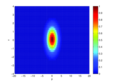
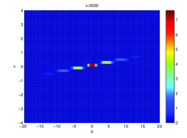
Figure 2: Initial condition: typical scale of $p$: $\sigma(p)=1.8$; typical scale of $v$: $\sigma(v)=0.9$; influence radius: $r=0.6$; length of each time step: $dt=0.005$ and totally 3000 period. x-axis is position and y-axis is velocity. The color reveals the density of the agents according to the right side color bar. At the beginning of the simulation, there is only one group; as the time goes by, the group starts to divide into several small groups. After 3000 periods, all agents have been divided into about 7 groups with most of the agents near the origin of the phase space.

3 Effects of typical scales of initial position and velocity on group-division phenomenon

As shown above, the mean field model matches the discrete simulation very well. To see this more clearly, we display the data projection on the position axis. An example of such a projection, shown in Figure.3, reveals the group-division phenomenon in both models — dash line and solid line represent mean field model and discrete model respectively. This comparison further validates the mean field model.

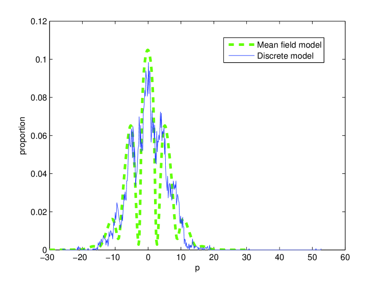
Figure 3: Initial condition: typical scale of $p$: $\sigma(p)=3$; typical scale of $v$: $\sigma(v)=1$; influence radius: $r=0.6$; length of each time step: $dt=0.005$; number of agents: $N=10000$; and totally 3000 period. x-axis is position and y-axis is the proportion of the agents in that position.

Next, we find that the group-division phenomenon is related to the typical scales of initial position and velocity, as well as the influence radius. Scale $\sigma(p)$ and $\sigma(v)$ with $r$, we get some further examples, which are shown in the following (Figure.4). Y-axis indicates $\lambda$, the ratio of the size of largest group and the whole group. Smaller $\lambda$ causes more obvious group-division phenomenon, and the group-division phenomenon will disappear when $\lambda$ approaching 1. Since the line goes up all the way, it illustrates that as $\sigma(p)$ increases, most of the agent will stay in the largest group so that group-division phenomenon becomes weaker. Also, three different $\sigma(v)$ curves indicates that as $\sigma(v)$ increases, the group-division phenomenon become more pronounced.

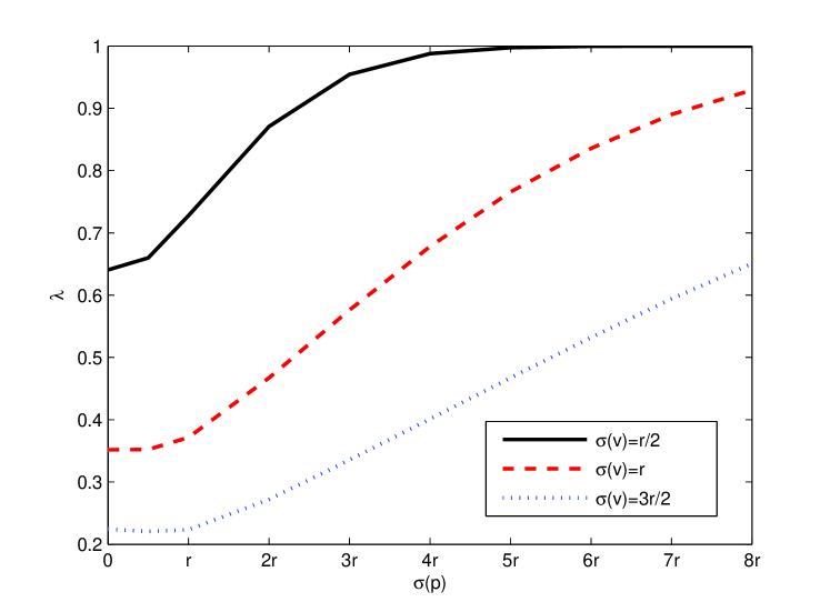
Figure 4: Initial condition: influence radius: $r=0.6$; length of each time step: $dt=0.005$; and totally 3000 period. x-axis is $\sigma(p)$, y-axis is $\lambda$, the ratio of the size of the largest group to the whole group.

4 Energy analysis

In this section, we analyze energetics of the group-division phenomenon. We find the energy-time curve has two stages connected by a sharp transition(see figure.5).

Define $K$ as the total kinetic energy of the system. Under the group-division phenomenon, label each group as:$\{g_{1},g_{2},...,g_{n}\}$, and the corresponding velocities of the groups as:$\{v_{g_{1}},v_{g_{2}},...,v_{g_{n}}\}$. $N_{g_{k}}$ defines the number of agents in group $g_{k}$. Thus:

$$K = \sum_{i=1}^{N}{v_{i}}^{2}$$ (2)

$$= \sum_{i=1}^{N}(({v_{i}}-\overline{v})+\overline{v})^{2}$$

$$= \sum_{i=1}^{N}({v_{i}}-\overline{v})^{2}+N\overline{v}^{2}$$

$$= \sum_{k=1}^{N}\sum_{i\in g_{k}}[({v_{i}}-{v_{g_{k}}})+({v_{g_{k}}}-\overline{v})]^{2}+N\overline{v}^{2}$$

$$= \sum_{k=1}^{N}\sum_{i\in g_{k}}[({v_{i}}-{v_{g_{k}}})^{2}+({v_{g_{k}}}-\overline{v})^{2}]+N\overline{v}^{2}$$

$$= \sum_{k=1}^{N}\sum_{i\in g_{k}}({v_{i}}-{v_{g_{k}}})^{2}+\sum_{k=1}^{N}N_{g_{k}}({v_{g_{k}}}-\overline{v})^{2}+N\overline{v}^{2}.$$

According to the last line (2), we write the kinetic energy into three terms, where $\sum_{k=1}^{N}\sum_{i\in g_{k}}({v_{i}}-{v_{g_{k}}})^{2}$ is the first term, $\sum_{k=1}^{N}N_{g_{k}}({v_{g_{k}}}-\overline{v})^{2}$ is the second term, and $N\overline{v}^{2}$ is the third term.

The first term is the relative kinetic energy of the agents with respect to the center of mass of corresponding groups; the second term is the relative kinetic energy of the groups with respect to the global center of mass; the third term is the kinetic energy of the global center of mass, which is almost constant from the symmetry of Figure.3.

At the beginning of the simulation, since we only have one large group:

$$\sum_{k=1}^{N}N_{g_{k}}({v_{g_{k}}}-\overline{v})^{2}=0.$$

At the end of the simulation, since we have several groups, and each agent in its group will have the same velocity (i.e.:${v_{i}}={v_{g_{k}}}$):

$$\sum_{k=1}^{N}\sum_{i\in g_{k}}({v_{i}}-{v_{g_{k}}})^{2}=0.$$

Therefore, the kinetic energy shifts from the first term to the second term, as it decreases monotonically from its initial value.

Moreover, since:

$${d({v_{i}}-{v_{g_{k}}})\over dt}=-(v_{i}-{v_{g_{k}}}),$$

solving this ODE yields:

$${v_{i}}={v_{g_{k}}}+{v_{0}}e^{-t}.$$

Therefore the first term could be written as:

$$\sum_{k=1}^{n}\sum_{i\in{g_{k}}}({v_{i}}-{v_{g_{k}}})^{2}=(\sum_{k=1}^{n}\sum_{i\in{g_{k}}}{v_{i_{0}}}^{2})\cdot e^{-2t}.$$ (3)

We consider the change of the variance of agent velocity, which can be interpreted as kinetic energy. By equation (3), we know that the kinetic energy decrease exponentially in the first stage, which is dominated by the first term of the equation. By taking the log of the variance, the slope of the corresponding curve is found to be close to -2. On the other hand, since we know that $v_{g_{k}}$ will finally be constant, the curve of kinetic energy should be a straight line after division is complete, so the log of the variance is still a straight line after division. Since we know that the kinetic energy shifts from the first term to the second term, we pick the point of the largest change in the semi-log variance during the process as the end of the group-division phenomenon.

During the process, the variance of velocity decreases exponentially (see Figure.5). We take the log of the variance of $v$(Y-axis in left figure), and consider its rate of change of slope. The maximum point of change of slope rate, which we take to be the end of division, is 195 (258) of the mean field model (discrete model). The difference of these two numbers mostly come from the random choice of initial data in the discrete model, so we consider the former one (195) is more accurate.

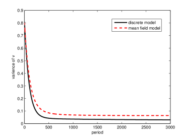
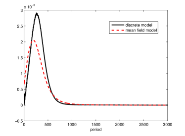
Figure 5: Initial condition: typical scale of $p$: $\sigma(p)=1.8$; typical scale of $v$: $\sigma(v)=0.9$; influence radius: $r=0.6$; length of each time step: $dt=0.5$ and totally 20000 period. For the left figure, X-axis shows the number of periods, Y-axis is the variance of velocity. The second derivation of the log of variance of velocity(Y-axis) in left figure gives the curve in the right figure.

5 Conclusion

In our paper, we propose an adaptive-velocity swarm model in which each agent not only adjusts its movement direction but also adjusts its speed as a function of its local neighbors in 1-dimensional space. Such a spatially 1-dimensional model is nonetheless capable of supporting a robust group-division phenomenon that moreover, depends strongly on just two key parameters of the initial swarm - its typical scales in the initial positions and velocities of the agents. Details of possible weak dependence on other properties of the initial swarm will emerge from future studies. Furthermore, we show that group-division typically occurs in two stages separated by the point in time whereby most of the kinetic energy has shifted from the first term to the second term. In the first stage, the whole group self-divides into several smaller groups, followed by the second stage in which each smaller group consolidates into one that has its own nearly constant velocity and direction, within the fixed radius of influence.

Some difficult but important problems of our model remain to be further investigated. For example, under what condition can we infer the same result in 2-dimensional and 3-dimensional space? What kind of behavior will emerge if certain agents have greater influence than others? In the more applied aspect, how do we control the motion of a swarm efficiently in our model? In addition, practical stability analysis of the mean field model discussed in this paper needs to be carried out.

References

- [1] Reynolds, Craig W. ”Flocks, herds and schools: A distributed behavioral model.” In ACM SIGGRAPH Computer Graphics, vol. 21, no. 4, pp. 25-34. ACM, 1987.
- [2] Vicsek, Tam s, Andr s Czir k, Eshel Ben-Jacob, Inon Cohen, and Ofer Shochet. ”Novel type of phase transition in a system of self-driven particles.” Physical Review Letters 75, no. 6 (1995): 1226.
- [3] Huepe, Cristi n, and Maximino Aldana. ”Intermittency and clustering in a system of self-driven particles.” Physical review letters 92, no. 16 (2004): 168701.
- [4] Moreau, Luc. ”Stability of multiagent systems with time-dependent communication links.” Automatic Control, IEEE Transactions on 50, no. 2 (2005): 169-182.
- [5] Toner, John, and Yuhai Tu. ”Long-range order in a two-dimensional dynamical XY model: how birds fly together.” Physical Review Letters 75, no. 23 (1995): 4326.
- [6] Aldana, Maximino, and Cristi n Huepe. ”Phase transitions in self-driven many-particle systems and related non-equilibrium models: a network approach.” Journal of Statistical Physics 112, no. 1-2 (2003): 135-153.
- [7] Nabet, Benjamin, Naomi E. Leonard, Iain D. Couzin, and Simon A. Levin. ”Dynamics of decision making in animal group motion.” Journal of nonlinear science 19, no. 4 (2009): 399-435.
- [8] Li, Wei, and Xiaofan Wang. ”Adaptive velocity strategy for swarm aggregation.” Physical Review E 75, no. 2 (2007): 021917.
- [9] Morale, Daniela, Vincenzo Capasso, and Karl Oelschl?ger. ”An interacting particle system modelling aggregation behavior: from individuals to populations.” Journal of Mathematical Biology 50, no. 1 (2005): 49-66.
- [10] D. Morale, ”Cellular automata and many-particles systems modeling aggregation behaviour among populations.” Int. J. Appl. Math. Comput. Sci. 10 (2000) 157 C173.
- [11] Burger, Martin, Vincenzo Capasso, and Daniela Morale. ”On an aggregation model with long and short range interactions.” Nonlinear Analysis: Real World Applications 8, no. 3 (2007): 939-958.
- [12] Sumpter, David, Jerome Buhl, Dora Biro, and Iain Couzin. ”Information transfer in moving animal groups.” Theory in biosciences 127, no. 2 (2008): 177-186.
- [13] Sumpter, David JT, and Stephen C. Pratt. ”Quorum responses and consensus decision making.” Philosophical Transactions of the Royal Society B: Biological Sciences 364, no. 1518 (2009): 743-753.
- [14] Cavagna, Andrea, Alessio Cimarelli, Irene Giardina, Giorgio Parisi, Raffaele Santagati, Fabio Stefanini, and Massimiliano Viale. ”Scale-free correlations in starling flocks.” Proceedings of the National Academy of Sciences 107, no. 26 (2010): 11865-11870.
- [15] Mann, Richard P. ”Bayesian inference for identifying interaction rules in moving animal groups.” PloS one 6, no. 8 (2011): e22827.
- [16] Parrish, Julia K., and Leah Edelstein-Keshet. ”Complexity, pattern, and evolutionary trade-offs in animal aggregation.” Science 284, no. 5411 (1999): 99-101.
- [17] Parrish, Julia K., Steven V. Viscido, and Daniel Gr nbaum. ”Self-organized fish schools: an examination of emergent properties.” The biological bulletin 202, no. 3 (2002): 296-305.
- [18] Eymard, R. Gallout, T. R. Herbin, R. (2000) The finite volume method Handbook of Numerical Analysis, Vol. VII, 2000, p. 713 C1020. Editors: P.G. Ciarlet and J.L. Lions.