[table]labelsep=period,labelfont=bf,rm [figure]labelfont=bf,labelsep=period UPV/EHU]  Nano-Bio Spectroscopy Group and ETSF Scientific Development Centre, Departamento de Física de Materiales, Universidad del País Vasco, CSIC-UPV/EHU-MPC and DIPC, Avenida de Tolosa 72, E-20018 San Sebastián, Spain Purdue]
  Department of Physics, Purdue University, 525 Northwestern Avenue, West Lafayette, IN 47907, USA Purdue]
  Department of Chemistry, Purdue University, 560 Oval Drive, West Lafayette, IN 47907, USA [Purdue]
  Department of Physics, Purdue University, 525 Northwestern Avenue, West Lafayette, IN 47907, USA UPV/EHU]  Nano-Bio Spectroscopy Group and ETSF Scientific Development Centre, Departamento de Física de Materiales, Universidad del País Vasco, CSIC-UPV/EHU-MPC and DIPC, Avenida de Tolosa 72, E-20018 San Sebastián, Spain

Stark Ionization of Atoms and Molecules within Density Functional Resonance Theory

  ABSTRACT: We show that the energetics and lifetimes of resonances of finite systems under an external electric field can be captured by Kohn–Sham density functional theory (DFT) within the formalism of uniform complex scaling. Properties of resonances are calculated self-consistently in terms of complex densities, potentials and wavefunctions using adapted versions of the known algorithms from DFT. We illustrate this new formalism by calculating ionization rates using the complex-scaled local density approximation and exact exchange. We consider a variety of atoms (H, He, Li and Be) as well as the H₂ molecule. Extensions are briefly discussed.
SECTION: Spectroscopy, Photochemistry, and Excited States
KEYWORDS: Resonances, Tunneling, Spectroscopy, Lasers, Excitations, Complex scaling, Open quantum systems.
 

This document is the unedited Author’s version of a Submitted Work that was subsequently accepted for publication in J.Phys.Chem.Lett., copyright © American Chemical Society after peer review. To access the final edited and published work see http://pubs.acs.org/doi/abs/10.1021/jz401110h.

The description of metastable compounds has been elusive to first-principles calculations due to the lack of a variational principle. The concepts of metastability and long-lived resonances (or tunneling processes) are closely related, and in the end we are facing the description of the lifetime of a given open quantum system. One approach to such calculations is the complex-scaling method, pioneered by Aguilar, Balslev and Combes^{1, 2}. Within this formalism, resonances appear as the result of a complex scaling $\mathbf{r}\rightarrow\mathbf{r}\mathrm{e}^{i\theta}$ of the real-space coordinates in the Hamiltonian. The method has been used to calculate resonance energies and lifetimes of negative ions of atoms³, as well as resonances induced by static electric fields^{4, 5}.

Applications have however generally been limited to small systems or systems with reduced dimensionality due to the computational difficulty of solving many-particle problems. A different approach must be taken to accommodate realistic systems with many electrons. Recently it has been proven that the low-lying metastable states of a given system can be described within a density functional framework once we allow for complex densities⁶. An analog of the Hohenberg–Kohn theorem then allows for the calculation of the lowest-energy resonance of a system. Based on this, the first Kohn–Sham density functional resonance theory (DFRT) calculations have since been published, although limited to 1D systems with one or two electrons^{7, 8}.

A notable ongoing development, termed complex DFT (CODFT), is based on complex absorbing potentials^{9, 10}. This method relies on the definition of an absorption zone outside the system boundary to calculate lifetimes based on how wavefunctions extend into the absorbing region. Another method is exterior complex scaling, where a complex coordinate scaling is applied outside of a certain radius¹¹.

The method presented in this Letter is based on uniform complex scaling, where all regions of space are treated equally. We present first-principles DFRT calculations of Stark resonance states and lifetimes in real 3D systems within exact exchange (EXX) and the local density approximation (LDA). We consider the H, He, Li, and Be atoms and the H₂ molecule within strong electric fields, extending the method beyond the model systems for which it has been demonstrated previously^{7, 8}. The implementation is open source and part of the DFT code Octopus^{12, 13}. Wavefunctions are represented on real-space grids, and atoms are represented by pseudopotentials. Atomic units are used throughout this article.

We describe first how complex scaling is incorporated within DFT, then present the major algorithmic steps involved. Finally we discuss the results.

The complex-scaling transformation $\mathbf{r}\rightarrow\mathbf{r}\mathrm{e}^{i\theta}$ changes the Hamiltonian of a system into a non-Hermitian operator $\hat{H}^{\theta}$, affecting bound and unbound eigenstates differently. The energy of any bound state is conserved, while that of a non-normalizable, unbound state changes. As $\theta$ is increased from 0, resonances can be uncovered from among the continuum as localized eigenstates of $\hat{H}^{\theta}$. From the corresponding complex eigenvalues $\epsilon=\epsilon_{\mathrm{res}}-i\Gamma/2$, the ionization rate is given by $\Gamma$; see e.g. the review by Reinhardt¹⁴.

Standard Kohn–Sham (KS) DFT is formulated as the minimization of an energy functional over a set of auxiliary single-particle states. Correspondingly we take the complex-valued Kohn–Sham energy functional⁸ to be

$$E_{\mathrm{res}}-i\frac{\Gamma}{2} =\mathrm{e}^{-i2\theta}\sum_{n}\int\psi_{n}^{\theta}(\mathbf{r})\left(-\frac{1}{2}\nabla^{2}\right)\psi_{n}^{\theta}(\mathbf{r})\,\mathrm{d}\mathbf{r}$$

$$\quad+\mathrm{e}^{-i\theta}\frac{1}{2}\int\int\frac{n^{\theta}(\mathbf{r})n^{\theta}(\mathbf{r}^{\prime})}{\|\mathbf{r}-\mathbf{r}^{\prime}\|}\,\mathrm{d}\mathbf{r}\,\mathrm{d}\mathbf{r}^{\prime}$$

$$\quad+E_{\mathrm{xc}}^{\theta}[n^{\theta}]+\int v_{\mathrm{ext}}^{\theta}(\mathbf{r})n^{\theta}(\mathbf{r})\,\mathrm{d}\mathbf{r},$$ (1)

where $E_{\mathrm{res}}$ is the resonance energy and $\Gamma$ the ionization rate inverse lifetime. $\Gamma$ represents a total over all metastable single-electron states in the system. Above we have introduced complex-scaled Kohn–Sham states $\psi_{n}^{\theta}(\mathbf{r})$, density $n^{\theta}(\mathbf{r})$, and operators $\hat{O}^{\theta}(\mathbf{r})$ (such as $v_{\mathrm{ext}}^{\theta}(\mathbf{r})$ and the kinetic operator), which are analytic continuations

$$\psi^{\theta}(\mathbf{r}) =\mathrm{e}^{i3\theta/2}\psi(\mathbf{r}\mathrm{e}^{i\theta}),$$ (2)

$$n^{\theta}(\mathbf{r}) =\sum_{n}[\psi_{n}^{\theta}(\mathbf{r})]^{2}=\mathrm{e}^{i3\theta}n(\mathbf{r}\mathrm{e}^{i\theta})$$ (3)

$$\hat{O}^{\theta}(\mathbf{r}) =\hat{O}(\mathbf{r}\mathrm{e}^{i\theta}),$$ (4)

of their unscaled equivalents. We have used that bra states are not conjugated¹⁵, and that left and right eigenstates are equal, since the complex-scaled Hamiltonian of a finite system is complex-symmetric. This is always the case when the initial, unscaled Hamiltonian contains only real terms. These definitions ensure that integrals such as matrix elements are unaffected by the scaling angle $\theta$ under appropriate conditions¹⁴. Thus (1) reduces to the ordinary KS energy functional if the system is bound.

For unbound systems the energy functional is complex and therefore does not possess a minimum. However the lowest resonance can still be obtained by requiring the functional to be stationary.⁶ Taking the derivative with respect to the wavefunctions $\psi_{n}^{\theta}(\mathbf{r})$ yields a set of KS equations:

$$\hat{H}^{\theta}\psi_{n}^{\theta}(\mathbf{r})=\left[-\frac{1}{2}\mathrm{e}^{-i2\theta}\nabla^{2}+v^{\theta}(\mathbf{r})\right]\psi_{n}^{\theta}(\mathbf{r})=\epsilon_{n}\psi_{n}^{\theta}(\mathbf{r}),$$ (5)

where the effective potential $v^{\theta}(\mathbf{r})$ is the sum of the complex-scaled Hartree, XC and external potentials⁸ $v^{\theta}(\mathbf{r})=v_{\mathrm{H}}^{\theta}(\mathbf{r})+v_{\mathrm{xc}}^{\theta}(\mathbf{r})+v_{\mathrm{ext}}^{\theta}(\mathbf{r})$. A self-consistency loop is then formulated from these quantities. For each calculation a fixed value of $\theta$ is chosen. $\theta$ should be large enough for the resonant states to emerge, but can otherwise be chosen to optimize the numerics.^{16, 17} In the DFRT calculations presented here, $\theta$ is chosen by testing different values with different grid spacings to find a combination with good numerical precision. This is similar to the convergence checks performed in standard DFT, but more important, as the numerical error must be made smaller than the imaginary part of the energy, which can be quite close to zero. For this reason a fine grid is required to calculate low ionization rates.

   

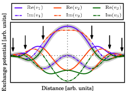
Figure 1: Real and imaginary parts of the three branches $v_{1}$, $v_{2}$ and $v_{3}$ of the LDA exchange potential generated by a complex-scaled Gaussian density. The branches are stitched together to form one continuous exchange potential, indicated by the shaded bands. Arrows indicate the branch points.

XC functionals $E_{\mathrm{xc}}^{\theta}[n^{\theta}]$ can be derived by analytic continuation consistently with Eqns. (2)–(4). Consider for example spin-paired LDA. The XC energy is complex-scaled by rotating the integration contour from the real axis into the complex plane:

$$E_{\mathrm{xc}}[n]=\int n(\mathbf{r})\epsilon(n(\mathbf{r}))\,\mathrm{d}\mathbf{r}=\int n(\mathbf{r}\mathrm{e}^{i\theta})\epsilon(n(\mathbf{r}\mathrm{e}^{i\theta}))\,\mathrm{d}\mathbf{r}\,\mathrm{e}^{i3\theta},$$ (6)

which is also a functional $E_{\mathrm{xc}}^{\theta}$ of $n^{\theta}(\mathbf{r})$ by (3). The potential follows as $v_{\mathrm{xc}}^{\theta}(\mathbf{r})=\delta E_{\mathrm{xc}}^{\theta}[n^{\theta}]/\delta n^{\theta}(\mathbf{r})$. Thus the exchange part of the potential becomes

$$v_{\mathrm{x}}^{\theta}(\mathbf{r})=-\left(\frac{3}{\pi}\right)^{1/3}\mathrm{e}^{-i\theta}[n^{\theta}(\mathbf{r})]^{1/3}=v_{\mathrm{x}}(\mathbf{r}\mathrm{e}^{i\theta}),$$ (7)

as in (4). Due to the complex cube root, the exchange potential is three-valued. However the potential is the complex continuation of a corresponding real potential for $\theta=0$, and so must remain continuous. Further, since the complex scaling operation leaves the origin $\mathbf{r}=0$ unaffected, $v_{\mathrm{x}}^{\theta}(0)$ must be real and independent of $\theta$. Starting at $\mathbf{r}=0$ we therefore evaluate $v_{\mathrm{x}}^{\theta}(\mathbf{r})$ as the principal branch of the cube root of the density. For some $\mathbf{r}$ the density may approach a branch point so the potential becomes discontinuous. This situation is illustrated in Figure 1, where the three branches, evaluated from a Gaussian density with $\theta=0.5$, have different colors. At a branch point, one can always choose another branch such that the resulting, stitched potential becomes continuous and yields the correct energy $E_{\mathrm{x}}^{\theta}[n^{\theta}]$ which does not depend on $\theta$.

Consider next the Perdew–Wang parametrization of correlation¹⁸. The correlation potential is expressed in terms of the Wigner–Seitz radius $\sqrt{r_{s}(\mathbf{r})}\sim[n(\mathbf{r})]^{-1/6}$ and takes the form

$$v_{c}(r_{s})=\epsilon_{c}(r_{s})-\frac{1}{3}\frac{\mathrm{d}\epsilon_{c}(r_{s})}{\mathrm{d}r_{s}}r_{s},$$ (8)

where

$$\epsilon_{c}(r_{s}) =-2A(1+\alpha_{1}r_{s})\ln\left(1+\frac{1}{Q_{1}(r_{s})}\right),$$ (9)

$$Q_{1}(r_{s}) =2A\sum_{i=1}^{4}\beta_{i}r_{s}^{i/2}.$$ (10)

Here $A$, $\alpha_{1}$ and $\beta_{1...4}$ are real constants. This expression is straightforward to complex-scale using the stitching method already presented. We first evaluate $\sqrt{r_{s}}$ at each point on the real-space grid by stitching $[n^{\theta}(\mathbf{r})]^{-1/6}$. Then the complex logarithm $\ln(1+1/Q_{1}(r_{s}))$ is stitched to obtain $\epsilon_{c}(r_{s})$. Other local or semilocal (GGA) functionals can be similarly complex-scaled.

 
 

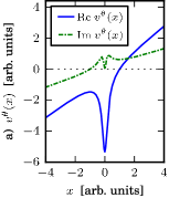
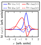
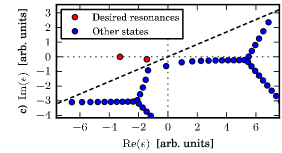
Figure 2: a) Real and imaginary parts of the complex-scaled potential. b) Real and imaginary parts of the lowest resonance wavefunctions. c) The spectrum. The dashed line $\arg z=\theta$ separates the two real resonances (red) with imaginary parts of $-2.6\times 10^{-3}$ and $-0.17$ from the remaining eigenstates (blue) which are artifacts of the simulation box or continuum.

One of the challenges in Kohn–Sham DFRT is to reliably determine which states should be occupied, as the complex eigenvalues have no natural ordering. Consider independent particles in 1D near an atom represented by a soft Coulomb potential with charge $Z$ in a uniform electric field of strength $F$. This system has the external potential $Fx\mathrm{e}^{i\theta}-Z/\sqrt{x^{2}\mathrm{e}^{i2\theta}+\alpha^{2}}$. Figure 2 shows a) the complex-scaled potential, b) wavefunctions and c) eigenvalues for $F=4$, $Z=4$, $\alpha=0.15$, and $\theta=0.4$ in a simulation box of size $10$. In the spectrum on Figure 2(c), the dashed line $\arg z=\theta$ divides the complex plane in two parts. On the upper left side there are two eigenvalues that correspond to physical resonances. These states would have been bound if no electric field had been applied to the system, but are now situated just below the real axis. Below the dashed line $\arg z=\theta$, the spectrum forms a system of lines. It has been demonstrated by Cerjan and co-workers^{19, 16} that the numerical range (the set of values $(\psi^{\theta}|H_{\mathrm{stark}}^{\theta}|\psi^{\theta})$ for all normalized states $\psi^{\theta}$) of the complex-scaled Stark Hamiltonian, and thus its entire continuous spectrum, falls within this region. The discrete eigenvalues above the line $\arg z=\theta$ can therefore be identified as originating from bound states in the isolated atom, and can now be assigned occupations in order of increasing real (or negative imaginary) part of the energy, while the remaining states are left unoccupied. In practical calculations using iterative eigensolvers, particularly when far away from self-consistency, eigenvalues originating from the continuum may appear above the line $\arg z=\theta$. As these states should not be occupied, we use a simple rule to identify them. They are occupied in ascending order of $\operatorname{Re}\epsilon+\alpha(\operatorname{Im}\epsilon)^{2}$, where $\alpha$ is a tunable parameter. The value $\alpha=2/\sin\theta$ generally works for the atoms considered here.

   

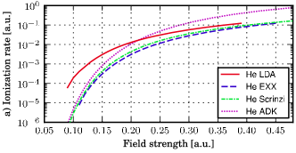
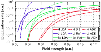
Figure 3: Ionization rates ($1\,\textrm{a.u.}\approx 4.13\times 10^{16}\,\mathrm{s}^{-1}$) of (a) He and (b) H, Li, and Be as a function of electric field strength ($1\,\textrm{a.u.}\approx 5.14\times 10^{11}\,\mathrm{V/m}$). Rates are calculated using DFRT (LDA or EXX) and the Ammosov–Delone–Krainov (ADK) method²⁰. Rates of H are also calculated by solving the complex-scaled Schrödinger equation. Accurate reference rates from first-principles methods are shown for He²¹, Li,²² and Be²³.

Like in standard DFT calculations, it is the outermost (valence) electrons that determine most properties of a system. Nuclear point charges cause numerical difficulties due to their central singularity. Pseudopotentials solve this problem by replacing the point charges by smooth charge distributions, while making sure to account properly for the core–valence interaction. Here we use the normconserving Hartwigsen–Goedecker–Hutter (HGH) pseudopotentials²⁴. They can be explicitly complex-scaled since they are parametrized as polynomials and Gaussians. In the calculations below, we use the potentials that include all electrons as valence electrons while only smoothening the nuclear potential (Li and Be have 3 and 4 valence electrons, respectively). With this choice the approach is demonstrated on systems with more than one occupied Kohn–Sham state. The approach is also compatible with standard frozen-core pseudopotentials.

Figure 3(a) shows the ionization rate for He as a function of electric field strength calculated using various methods. The reference results are based on direct solution of the complex-scaled two-particle Schrödinger equation and thus represent the closest to an exact calculation²¹. The DFRT rates $\Gamma$ for LDA and EXX are obtained directly from (1) after solving the KS equations (5) self-consistently for the complex density using $\theta=0.35$. A value of $\theta$ is suitable if it is large enough to localize the resonant KS states, and if the results converge rapidly with grid spacing. A very fine grid spacing of 0.08 a.u. is still needed to converge the lowest rates. The LDA substantially overestimates the ionization rate, particularly for small fields, while EXX is in very good agreement with the reference. EXX results are obtained by setting the exchange energy to minus half the Hartree energy, which is exact for two-electron systems.

Also shown are results from the Ammosov–Delone–Krainov (ADK) method²⁰. This is a simple approximation for ionization rates in atoms, based on the atomic ionization potential. ADK is accurate for low fields because the ionization rate is strongly linked to the ionization potential in this limit. However it greatly overestimates rates for large fields. We attribute the inaccuracy of LDA for low fields to its well-known underestimation of ionization potentials, taken as minus the energy of the highest occupied Kohn–Sham orbital (0.57 Hartree from LDA, versus 0.92 from EXX and 0.90 from experiment). This error of LDA is ultimately linked to the exponential rather than Coulomb-like decay of the potential.²⁵ Note that more accurate ionization potentials can be calculated by subtracting the total energy of the charged and the neutral system. Ionization rates based on this method have been presented with CODFT⁹.

Similarly calculated ionization rates with LDA and ADK are shown for H, Li, and Be in Figure 3(b) along with reference values for H from ordinary one-particle calculations, and for Li²² and Be²³. Generally the atoms with lower atomization potentials have higher ionization rates, and again a large discrepancy shows between ADK and LDA for low fields.

   

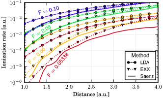
Figure 4: Ionization rate of H₂ as a function of internuclear distance. Different methods are denoted by different line and point styles, while colors denote different static field strengths in atomic units.

Figure 4 shows ionization rates for the H₂ molecule as a function of internuclear distance calculated for different field strengths with LDA and EXX. The molecular axis is parallel to the electric field. The nuclei are described as fixed point particles, so only the static electron ionization yield is calculated. The reference calculations by Saenz²⁶ correspond to an accurate solution of the two-particle complex-scaled Schrödinger equation.

H₂ in the dissociation limit is a pathological case in DFT as the system is dominated by strong static correlations that most functionals fail to capture. In this limit the system consists of two isolated, charge neutral atoms. A static calculation with an electric field will produce a different solution where both electrons reside on the atom favored by the field, although the situation at intermediate distances as here is more complicated.

LDA again overestimates ionization rates, particularly for short bond lengths. For large field strength and short bond lengths, the agreement between EXX and the reference is almost perfect. However ionization rates on the order of $10^{-5}$ a.u. lose accuracy due to the numerical dependence of energy on $\theta$. This error can be eliminated by optimizing the choice of $\theta$ and using a more fine grid spacing¹⁶ (0.1 Bohr with $\theta=0.22$ for the data points in question). We attribute most of the disagreement at short bond lengths between EXX and the reference to this error.

At large bond lengths and large field strength, the EXX agrees well with the reference. This corresponds to the case where both electrons reside mostly on the same atom. For smaller field strengths the system corresponds more closely to the strongly correlated case, and the error is larger.

The accuracy of the XC approximation is clearly a determining factor for the quantitative success of DFRT. We have here considered very simple functionals, and in particular LDA exhibits large errors. Phenomena of excited states depend intricately on the decay properties of the potential far from the system, which are difficult to describe with semilocal functionals. A promising method to solve this problem is to introduce a fictitious “XC density” which defines a correction to the XC potential, giving it a Coulomb-like decay.²⁷ This can greatly improve the accuracy of ionization rates. We expect the derivation of improved XC functionals for DFRT to be one of the next major steps in the development of this method.

The presented calculations demonstrate the reliability and performance of DRFT for realistic atoms and dimers. The extension to other molecular systems and nanostructures is straightforward, opening the path towards a systematic study of the electronic and structural properties of metastable complexes. Furthermore, DFRT has implications for the discussion and analysis of resonances in molecular electronics as well as to the description of intermediates in surface–molecule interactions, as the method introduces decay processes in a natural way into the widely used first-principles density-functional framework.

A future goal is to enable DFRT calculations for time-dependent systems, where time propagation can be started from statically determined resonant states. This paves the road to tackle dynamical processes through metastable intermediates, as seen in the recently available ultrafast and ultraintense laser probes that allow to extract temporal and spatial information of electron and ion dynamics²⁸ as well as imaging.^{29, 30}

AUTHOR INFORMATION

Corresponding Authors

*E-mail: asklarsen@gmail.com (A.H.L.);
umberto.degiovannini@ehu.es (U.D.G.);
awasser@purdue.edu (A.W.);
angel.rubio@ehu.es (A.R.)

Notes

The authors declare no competing financial interest.

REFERENCES

- Aguilar and Combes 1971 Aguilar, J.; Combes, J. A Class of Analytic Perturbations for One-Body Schrödinger Hamiltonians. Commun. Math. Phys. 1971, 22, 269–279
- Balslev and Combes 1971 Balslev, E.; Combes, J. Spectral Properties of Many-Body Schrödinger Operators With Dilatation-Analytic Interactions. Commun. Math. Phys. 1971, 22, 280–294
- Moiseyev and Corcoran 1979 Moiseyev, N.; Corcoran, C. Autoionizing States of and Using the Complex-Scaling Method. Phys. Rev. A 1979, 20, 814–817
- Reinhardt 1976 Reinhardt, W. P. Method of Complex Coordinates: Application to the Stark Effect in Hydrogen. Int. J. Quantum Chem. 1976, 10, 359–367
- Herbst and Simon 1978 Herbst, I. W.; Simon, B. Stark Effect Revisited. Phys. Rev. Lett. 1978, 41, 67–69
- Wasserman and Moiseyev 2007 Wasserman, A.; Moiseyev, N. Hohenberg-Kohn Theorem for the Lowest-Energy Resonance of Unbound Systems. Phys. Rev. Lett. 2007, 98, 093003
- Whitenack and Wasserman 2010 Whitenack, D. L.; Wasserman, A. Resonance Lifetimes from Complex Densities. J. Phys. Chem. Lett. 2010, 1, 407–411
- Whitenack and Wasserman 2011 Whitenack, D. L.; Wasserman, A. Density Functional Resonance Theory of Unbound Electronic Systems. Phys. Rev. Lett. 2011, 107, 163002
- Zhou and Ernzerhof 2012 Zhou, Y.; Ernzerhof, M. Calculating the Lifetimes of Metastable States with Complex Density Functional Theory. J. Phys. Chem. Lett. 2012, 3, 1916–1920
- Zhou and Ernzerhof 2012 Zhou, Y.; Ernzerhof, M. Open-System Kohn-Sham Density Functional Theory. J. Chem. Phys. 2012, 136, 094105
- Simon 1979 Simon, B. The Definition of Molecular Resonance Curves by the Method of Exterior Complex Scaling. Phys. Lett. A 1979, 71, 211–214
- Marques et al. 2003 Marques, M. A.; Castro, A.; Bertsch, G. F.; Rubio, A. Octopus: A First-Principles Tool For Excited Electron–Ion Dynamics. Comput. Phys. Commun. 2003, 151, 60–78
- Castro et al. 2006 Castro, A.; Appel, H.; Oliveira, M.; Rozzi, C. A.; Andrade, X.; Lorenzen, F.; Marques, M. A. L.; Gross, E. K. U.; Rubio, A. Octopus: A Tool for the Application of Time-Dependent Density Functional Theory. Phys. Status Solidi B 2006, 243, 2465–2488
- Reinhardt 1982 Reinhardt, W. P. Complex Coordinates in the Theory of Atomic and Molecular Structure and Dynamics. Annu. Rev. Phys. Chem. 1982, 33, 223–255
- Moiseyev et al. 1978 Moiseyev, N.; Certain, P.; Weinhold, F. Resonance Properties of Complex-Rotated Hamiltonians. Mol. Phys. 1978, 36, 1613–1630
- Cerjan et al. 1978 Cerjan, C.; Hedges, R.; Holt, C.; Reinhardt, W. P.; Scheibner, K.; Wendoloski, J. J. Complex Coordinates and the Stark Effect. Int. J. Quantum Chem. 1978, 14, 393–418
- Whitenack and Wasserman 2012 Whitenack, D. L.; Wasserman, A. Density Functional Resonance Theory: Complex Density Functions, Convergence, Orbital Energies, and Functionals. J. Chem. Phys. 2012, 136, 164106
- Perdew and Wang 1992 Perdew, J. P.; Wang, Y. Accurate and Simple Analytic Representation of the Electron-Gas Correlation Energy. Phys. Rev. B 1992, 45, 13244–13249
- Cerjan et al. 1978 Cerjan, C.; Reinhardt, W. P.; Avron, J. E. Spectra of Atomic Hamiltonians in DC Fields: Use of the Numerical Range to Investigate the Effect of a Dilatation Transformation. J. Phys. B: At. Mol. Phys. 1978, 11, L201–L205
- Ammosov et al. 1986 Ammosov, M. V.; Delone, N. B.; Krainov, V. P. Tunnel Ionization of Complex Atoms and Atomic Ions in a Varying Electromagnetic-Field. Zh. Éksp. Teor. Fiz. 1986, 91, 2008–2013
- Scrinzi et al. 1999 Scrinzi, A.; Geissler, M.; Brabec, T. Ionization Above the Coulomb Barrier. Phys. Rev. Lett. 1999, 83, 706–709
- Nicolaides and Themelis 1993 Nicolaides, C. A.; Themelis, S. I. Theory and Computation of Electric-Field-Induced Tunneling Rates of Polyelectronic Atomic States. Phys. Rev. A 1993, 47, 3122–3127
- Themelis and Nicolaides 2000 Themelis, S. I.; Nicolaides, C. A. Complex Energies and the Polyelectronic Stark Problem. J. Phys. B: At., Mol. Opt. Phys. 2000, 33, 5561–5580
- Hartwigsen et al. 1998 Hartwigsen, C.; Goedecker, S.; Hutter, J. Relativistic Separable Dual-Space Gaussian Pseudopotentials from H to Rn. Phys. Rev. B 1998, 58, 3641–3662
- van Leeuwen and Baerends 1994 van Leeuwen, R.; Baerends, E. J. Exchange-correlation potential with correct asymptotic behavior. Phys. Rev. A 1994, 49, 2421–2431
- Saenz 2000 Saenz, A. Enhanced Ionization of Molecular Hydrogen in Very Strong Fields. Phys. Rev. A 2000, 61, 051402
- Andrade and Aspuru-Guzik 2011 Andrade, X.; Aspuru-Guzik, A. Prediction of the Derivative Discontinuity in Density Functional Theory from an Electrostatic Description of the Exchange and Correlation Potential. Phys. Rev. Lett. 2011, 107, 183002
- Shafir et al. 2012 Shafir, D.; Soifer, H.; Bruner, B. D.; Dagan, M.; Mairesse, Y.; Patchkovskii, S.; Ivanov, M. Y.; Smirnova, O.; Dudovich, N. Resolving the Time When an Electron Exits a Tunnelling Barrier. Nature 2012, 485, 343–346
- Zhou et al. 2012 Zhou, X.; Ranitovic, P.; Hogle, C. W.; Eland, J. H. D.; Kapteyn, H. C.; Murnane, M. M. Probing and Controlling Non-Born-Oppenheimer Dynamics in Highly Excited Molecular Ions. Nat. Phys. 2012, 8, 232–237
- Hensley et al. 2012 Hensley, C. J.; Yang, J.; Centurion, M. Imaging of Isolated Molecules with Ultrafast Electron Pulses. Phys. Rev. Lett. 2012, 109, 133202