APCTP Pre2013-011

Higher order non-linear parameters with PLANCK

Jinn-Ouk Gong^1,2 and Tomo Takahashi³

¹Asia Pacific Center for Theoretical Physics, Pohang 790-784, Korea
²Department of Physics, Postech, Pohang 790-784, Korea
³Department of Physics, Saga University, Saga 840-8502, Japan

We investigate how higher order non-linear parameters affect lower order ones through loop effects. We calculate the loop corrections up to two-loops and explicitly show that the tree contribution is stable against loop terms in most cases. We argue that, nevertheless, observational constraints on non-linear parameters such as $f_{\rm NL}$ and $\tau_{\rm NL}$ can also give a limit even for higher order ones due to the loop contribution. We discuss these issues for both single-source and multi-source cases.

1 Introduction

Recent PLANCK data have well measured the quantities which characterize the nature of primordial density fluctuations with unprecedented accuracy [1, 2]. Among them, the non-linear parameter $f_{\rm NL}$, which parametrizes the amplitude of the bispectrum, has been of great interest since it was regarded as a critical test of inflation, and the PLANCK team obtained much severer constraints than pre-PLANCK observations. For the so-called local type, both $f_{\rm NL}$ and $\tau_{\rm NL}$, which characterizes the size of the trispectrum for a certain configuration of wave numbers, are now severely constrained as [2]

$$-8.9< f_{\rm NL}^{\rm(local)}<14.3\,,$$ (1)

$$\tau_{\rm NL}<2800\,,$$ (2)

both at a 95% confidence level, which is consistent with Gaussian density fluctuations. Since the standard (single-field) inflation models predict almost Gaussian ones, they passed a critical test with the PLANCK results. Furthermore, other models of primordial fluctuations such as those utilizing a spectator field, like the curvaton model [5], modulated reheating model [6] and so on, which have been attracting attention due to their ability to produce large non-Gaussianity, are also still viable since they can also give $f_{\rm NL}\sim\mathcal{O}(1)$ in some parameter ranges.

However, one can also speculate a model in which the signature of non-Gaussianity comes not from the bispectrum but from higher order parameters such as $g_{\rm NL}$. In particular, in some models, large values of $g_{\rm NL}$ are possible even when $f_{\rm NL}$ satisfies the PLANCK constraint [7]. In fact, when $g_{\rm NL}$ is large, it can contribute to the total value of $f_{\rm NL}$ through higher order correlation functions, or what is often called loop correction [8]. In general, higher order non-linear parameters can also affect lower order ones through the loop corrections, which may enable us to probe higher order non-linear parameters by using observational constraints on lower order counterparts such as $f_{\rm NL}$ and $\tau_{\rm NL}$. Since PLANCK put a stringent constraint on $f_{\rm NL}$ and even on $\tau_{\rm NL}$, it would be interesting to see to what extent one can probe higher order non-linear parameters using the PLANCK constraints, which is the main topic in this article.

In the next section, we summarize the formalism and set our notations. We also give the explicit expressions of $f_{\rm NL},\tau_{\rm NL}$, and $g_{\rm NL}$, including the loop correction up to two-loops. After obtaining the expressions for these non-linear parameters, in Section 3, we investigate the constraints for higher order non-linear parameters using the PLANCK constraints on $f_{\rm NL}$ and $\tau_{\rm NL}$. The final section is devoted to conclusion of this article and discussion.

2 Formalism

In this section, we give a formalism and the expressions for non-linear parameters including the loop contributions. We focus on the local-type model, in which the curvature perturbation on the uniform density slice $\zeta$ may be expanded as

$$\zeta =\zeta_{g}+\frac{3}{5}f_{\rm NL}\zeta_{g}^{2}+\left(\frac{3}{5}\right)^{2}g_{\rm NL}\zeta_{g}^{3}+\left(\frac{3}{5}\right)^{3}h_{\rm NL}\zeta_{g}^{4}+\left(\frac{3}{5}\right)^{4}i_{\rm NL}\zeta_{g}^{5}+\left(\frac{3}{5}\right)^{5}j_{\rm NL}\zeta_{g}^{6}+\left(\frac{3}{5}\right)^{6}k_{\rm NL}\zeta_{g}^{7}+\cdots$$

$$\equiv\zeta^{(1)}+\zeta^{(2)}+\zeta^{(3)}+\zeta^{(4)}+\zeta^{(5)}+\zeta^{(6)}+\zeta^{(7)}+\cdots\,,$$ (3)

where we have defined explicitly the “bare” non-linear parameters as above and included up to the 7th order: this is required to calculate the corrections up to two-loop order for the trispectrum. For this perturbative expansion to be valid, we may naturally require $\zeta^{(n)}\gtrsim\zeta^{(n+1)}$. Thus, with $\zeta_{g}\sim 2\times 10^{-5}$, we obtain a generous bound for each non-linear parameter smaller than $10^{4}$-$10^{5}$. Notice that one may relax this assumption in such a way that all the non-linear terms are of the same order of magnitude, $\zeta^{(2)}\sim\zeta^{(3)}\sim\zeta^{(4)}\cdots$, à la general slow-roll approximation [10]. In this case, the higher order non-linear parameters may be far larger than $10^{5}$. However, more generally, for such a hierarchy we need very elaborated models and we do not consider this possibility here.

The power spectrum $P_{\zeta}(k)$, bispectrum $B_{\zeta}(k_{1},k_{2},k_{3})$, and trispectrum $T_{\zeta}(k_{1},k_{2},k_{3},k_{4})$ are defined as

$$\left\langle\zeta(\textbf{\em k}_{1})\zeta(\textbf{\em k}_{2})\right\rangle \equiv(2\pi)^{3}\delta^{(3)}(\textbf{\em k}_{1}+\textbf{\em k}_{2})P_{\zeta}(k_{1})\,,$$ (4)

$$\left\langle\zeta(\textbf{\em k}_{1})\zeta(\textbf{\em k}_{2})\zeta(\textbf{\em k}_{3})\right\rangle \equiv(2\pi)^{3}\delta^{(3)}(\textbf{\em k}_{1}+\textbf{\em k}_{2}+\textbf{\em k}_{3})B_{\zeta}(k_{1},k_{2},k_{3})\,,$$ (5)

$$\left\langle\zeta(\textbf{\em k}_{1})\zeta(\textbf{\em k}_{2})\zeta(\textbf{\em k}_{3})\zeta(\textbf{\em k}_{4})\right\rangle \equiv(2\pi)^{3}\delta^{(3)}(\textbf{\em k}_{1}+\textbf{\em k}_{2}+\textbf{\em k}_{3}+\textbf{\em k}_{4})\,T_{\zeta}(k_{1},k_{2},k_{3},k_{4})\,.$$ (6)

Below we explicitly give the expressions for these spectra including the corrections up to two-loops, and we will see the effects of the higher order non-linear parameters through these loops.

2.1 Power spectrum

Introducing the notation

$$\left\langle\zeta^{(i)}(\textbf{\em k})\zeta^{(j)}(\textbf{\em q})\right\rangle+\text{possible perm}=(2\pi)^{3}\delta^{(3)}(\textbf{\em k}+\textbf{\em q})P_{\zeta}^{(ij)}(k)\,,$$ (7)

which represents the contribution from the correlation function of the $i$th- and $j$th order terms in (2), the power spectrum up to two-loop corrections is given by

$$P_{\zeta}(k)=P_{\zeta}^{(11)}+P_{\zeta}^{(13)}+P_{\zeta}^{(22)}+P_{\zeta}^{(15)}+P_{\zeta}^{(24)}+P_{\zeta}^{(33)}\,,$$ (8)

where $P_{\zeta}^{(11)}$ gives the tree term, $P_{\zeta}^{(22)}$ and $P_{\zeta}^{(13)}$ constitute one-loop [11] and $P_{\zeta}^{(15)},P_{\zeta}^{(24)}$, and $P_{\zeta}^{(33)}$ correspond to two-loop corrections. Explicit expressions for these terms are given in Appendix A. Writing the loop corrections in terms of the non-linear parameter and the tree power spectrum explicitly, we find

$$P_{\zeta}(k) =P_{\zeta}^{(11)}(k)\left\{1+\left(\frac{3}{5}\right)^{2}\left(4f_{\rm NL}^{2}+6g_{\rm NL}\right){\cal P}_{\zeta}(L^{-1})\log(kL)\right.$$

$$\left.\hskip 56.9055pt+\left(\frac{3}{5}\right)^{4}\left(48f_{\rm NL}h_{\rm NL}+45g_{\rm NL}^{2}+30i_{\rm NL}\right)\left[{\cal P}_{\zeta}(L^{-1})\log(kL)\right]^{2}\right\}\,,$$ (9)

where $L$ is a large fictitious box size in which the Fourier modes of the curvature perturbation are taken and we have assumed ${\cal P}_{\zeta}\equiv k^{3}P_{\zeta}^{(11)}/\left(2\pi^{2}\right)\sim 2.5\times 10^{-9}$ remains nearly scale invariant over this box. Over the observable scales, the logarithm gives ${\cal O}(1)$.

2.2 Bispectrum

The bispectrum up to two-loop corrections is given by

$$B_{\zeta}(k_{1},k_{2},k_{3})= B_{\zeta}^{(112)}$$

$$+B_{\zeta}^{(114)}+B_{\zeta}^{(123)}+B_{\zeta}^{(222)}$$

$$+B_{\zeta}^{(116)}+B_{\zeta}^{(125)}+B_{\zeta}^{(134)}+B_{\zeta}^{(224)}+B_{\zeta}^{(233)}\,,$$ (10)

where we have defined the notation, and likewise for the case of the power spectrum,

$$\left\langle\zeta^{(i)}(\textbf{\em k}_{1})\zeta^{(j)}(\textbf{\em k}_{2})\zeta^{(k)}(\textbf{\em k}_{3})\right\rangle+\text{possible perms}=(2\pi)^{3}\delta^{(3)}(\textbf{\em k}_{1}+\textbf{\em k}_{2}+\textbf{\em k}_{3})B_{\zeta}^{(ijk)}\,.$$ (11)

In (2.2), the first, second and third lines on the right hand side correspond to the tree, one-loop and two-loop contributions, respectively. Explicit expressions for these terms are given in Appendix B. Putting everything together, $f_{\rm NL}$ in the squeezed limit including up to two-loop correction is given by

$$f_{\rm NL}^{\rm(tot)}\equiv \frac{5}{12}\lim_{k_{3}\to 0}\frac{B_{\zeta}(k_{1},k_{2},k_{3})}{P_{\zeta}(k_{1})P_{\zeta}(k_{3})}$$

$$= f_{\rm NL}+\left(\frac{3}{5}\right)^{3}\left(-\frac{20}{3}f_{\rm NL}^{3}+10f_{\rm NL}g_{\rm NL}+10h_{\rm NL}\right)\left[{\cal P}_{\zeta}(L^{-1})\log(kL)\right]$$

$$+\left(\frac{3}{5}\right)^{5}\left(\frac{80}{3}f_{\rm NL}^{5}-80f_{\rm NL}^{3}g_{\rm NL}-40f_{\rm NL}^{2}h_{\rm NL}+45f_{\rm NL}g_{\rm NL}^{2}+150f_{\rm NL}i_{\rm NL}\right.$$

$$\left.\hskip 56.9055pt+180g_{\rm NL}h_{\rm NL}+75j_{\rm NL}\right)\left[{\cal P}_{\zeta}(L^{-1})\log(kL)\right]^{2}\,.$$ (12)

Notice that $f_{\rm NL}$ on the right hand side of the above expression is the “bare” $f_{\rm NL}$ appearing in (2) which should not be confused with $f_{\rm NL}^{\rm(tot)}$, that includes loop corrections.

2.3 Trispectrum

For the trispectrum, including up to two-loop corrections, we obtain

$$T_{\zeta}(k_{1},k_{2},k_{3},k_{4})$$

$$= T_{\zeta}^{(1113)}+T_{\zeta}^{(1122)}$$

$$+T_{\zeta}^{(1115)}+T_{\zeta}^{(1124)}+T_{\zeta}^{(1133)}+T_{\zeta}^{(1223)}+T_{\zeta}^{(2222)}$$

$$+T_{\zeta}^{(1117)}+T_{\zeta}^{(1126)}+T_{\zeta}^{(1135)}+T_{\zeta}^{(1144)}+T_{\zeta}^{(1225)}+T_{\zeta}^{(1234)}+T_{\zeta}^{(1333)}+T_{\zeta}^{(2224)}+T_{\zeta}^{(2233)}\,,$$

where the first, second and third lines on the right hand side correspond to the tree, one-loop and two-loop contributions, respectively. Here we have again introduced a notation $T_{\zeta}^{(ijkl)}$ as

$$\left\langle\zeta^{(i)}(\textbf{\em k}_{1})\zeta^{(j)}(\textbf{\em k}_{2})\zeta^{(k)}(\textbf{\em k}_{3})\zeta^{(l)}(\textbf{\em k}_{4})\right\rangle+\text{possible perms}=(2\pi)^{3}\delta^{(3)}(\textbf{\em k}_{1}+\textbf{\em k}_{2}+\textbf{\em k}_{3}+\textbf{\em k}_{4})T_{\zeta}^{(ijkl)}\,.$$ (14)

Explicit expressions for these terms are given in Appendix C.

There are two non-linear parameters corresponding to different dependences on $k_{ij}\equiv|\textbf{\em k}_{i}+\textbf{\em k}_{j}|$. Collecting $k_{ij}$ dependence in the trispectrum, $\tau_{\rm NL}$ is defined in the collapsed limit, including two-loop corrections, as

$$\tau_{\rm NL}^{\text{(tot)}}= \frac{1}{4}\lim_{k_{12}\to 0}\frac{T_{\zeta}\text{ with $k_{ij}$ dependence}}{P_{\zeta}(k_{1})P_{\zeta}(k_{3})P_{\zeta}(k_{12})}$$

$$= \left(\frac{5}{6}f_{\rm NL}\right)^{2}+\left(\frac{3}{5}\right)^{4}\left(-32f_{\rm NL}^{4}+48f_{\rm NL}^{2}g_{\rm NL}+36g_{\rm NL}^{2}+48f_{\rm NL}h_{\rm NL}\right)\left[{\cal P}_{\zeta}(L^{-1})\log(kL)\right]$$

$$+\left(\frac{3}{5}\right)^{6}\left(192f_{\rm NL}^{6}-576f_{\rm NL}^{4}g_{\rm NL}+1404f_{\rm NL}^{2}g_{\rm NL}^{2}-384f_{\rm NL}^{3}h_{\rm NL}+3456f_{\rm NL}g_{\rm NL}h_{\rm NL}\right.$$

$$\left.\hskip 51.21504pt+720h_{\rm NL}^{2}+720f_{\rm NL}^{2}i_{\rm NL}+720g_{\rm NL}i_{\rm NL}+360f_{\rm NL}j_{\rm NL}\right)\left[{\cal P}_{\zeta}(L^{-1})\log(kL)\right]^{2}$$ (15)

On the other hand, another trispectrum parameter $g_{\rm NL}$ is defined for those without $k_{ij}$ dependence in the doubly squeezed limit as

$$g_{\rm NL}^{\text{(tot)}}= \frac{25}{108}\lim_{k_{1},k_{2}\to 0}\frac{T_{\zeta}\text{ without $k_{ij}$ dependence}}{P_{\zeta}(k_{1})P_{\zeta}(k_{2})P_{\zeta}(k_{3})}$$

$$= g_{\rm NL}+\left(\frac{3}{5}\right)^{2}\left(-9g_{\rm NL}^{2}+24f_{\rm NL}h_{\rm NL}+10i_{\rm NL}\right)\left[{\cal P}_{\zeta}(L^{-1})\log(kL)\right]$$

$$+\left(\frac{3}{5}\right)^{4}\left(-48f_{\rm NL}^{4}g_{\rm NL}+180f_{\rm NL}^{2}g_{\rm NL}^{2}+54g_{\rm NL}^{3}-192f_{\rm NL}^{3}h_{\rm NL}+288f_{\rm NL}g_{\rm NL}h_{\rm NL}\right.$$

$$\left.\hskip 51.21504pt+144h_{\rm NL}^{2}+240f_{\rm NL}^{2}i_{\rm NL}+225g_{\rm NL}i_{\rm NL}+360f_{\rm NL}j_{\rm NL}+105k_{\rm NL}\right)\left[{\cal P}_{\zeta}(L^{-1})\log(kL)\right]^{2}.$$

With these machineries, in the next section, we discuss implications of constraints on $f_{\rm NL}^{\rm(tot)}$ and $\tau_{\rm NL}^{\rm(tot)}$ for higher order non-linear parameters.

3 Probing higher order non-linear parameters

3.1 Single source case

First we consider $f_{\rm NL}^{\text{(tot)}}$ as a function of bare $f_{\rm NL}$ with the other non-linear parameters being fixed (see later), which is shown in the left panel of Fig. 1. Up to $f_{\rm NL}\sim 10^{4}$, the tree result, i.e. $f_{\rm NL}^{\text{(tot)}}=f_{\rm NL}$, holds very accurately. However, for $f_{\rm NL}\sim 10^{4}$ if we truncate at one-loop level, the tree result $f_{\rm NL}$ is canceled by the contribution from the $f_{\rm NL}^{3}$ term since the sign is opposite. Meanwhile if we further include the two-loop contributions, such a cancellation does not occur and one may conclude that the truncation at a certain order may lead to misevaluation of non-linear parameters. But at this large value of the bare $f_{\rm NL}$ the perturbativity of the expansion (2) is broken, i.e. the hierarchy $\zeta^{(1)}\gtrsim\zeta^{(2)}$ does not hold, and we can no longer be sure that the loop corrections are under control. In other words, as long as the bare $f_{\rm NL}$ is not too large to harm the perturbative expansion (2), the tree term is absolutely dominating over loop corrections. We can draw similar results for $\tau_{\rm NL}$ and $g_{\rm NL}$ shown in the middle and right panels of Fig. 1.

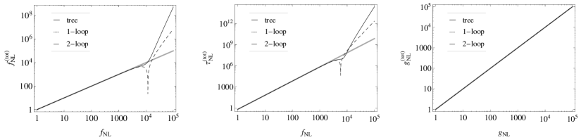
Figure 1: Plot of $f_{\rm NL}^{\rm(tot)}$ (left), $\tau_{\rm NL}^{\rm(tot)}$ (middle) and $g_{\rm NL}^{\rm(tot)}$ (right) as a function of bare non-linear parameters. Here absolute values are plotted. In all panels, we assume $h_{\rm NL}=10^{3}$ and set all higher non-linear parameters to be zero. In the left and middle panels, we set $g_{\rm NL}=10^{3}$, and in the right panel, $f_{\rm NL}=10^{3}$ is assumed. However, as long as we set all non-linear parameters less than $10^{5}$, we obtain more or less the same results. Notice that at large $f_{\rm NL}$, the sign of $f_{\rm NL}^{\rm(tot)}$ and $\tau_{\rm NL}^{\rm(tot)}$ changes from positive to negative and a cancellation occurs to give $f_{\rm NL}^{\rm(tot)}$ and $\tau_{\rm NL}^{\rm(tot)}$ vanishing at one-loop level, however, when two-loop corrections are included, such a cancellation does not occur.

Next, we show the contours of $f_{\rm NL}^{\text{(tot)}}$, $\tau_{\rm NL}^{\text{(tot)}}$, and $g_{\rm NL}^{\text{(tot)}}$ as functions of bare $f_{\rm NL}$, $g_{\rm NL}$, and $h_{\rm NL}$ in Fig 2. The values of other non-linear parameters assumed in the figure are shown in the caption. As seen from the plots, the loop corrected values of these non-linear parameters are almost determined by the corresponding bare ones, as long as higher order non-linear parameters are not too large to respect the hierarchy of the non-linear expansion (2). We note here that in principle, higher order non-linear parameters can be constrained from observations of $f_{\rm NL}^{\text{(tot)}}$, although their constraints are very weak. Nevertheless, it is interesting to see that, adopting $\tau_{\rm NL}<2800$ (95 % C.L. from PLANCK data), we obtain $g_{\rm NL}<5\times 10^{5}$, which is almost the same as the actual constraint from WMAP9, $g_{\rm NL}=(-3.3\pm 2.2)\times 10^{5}~{}{\rm(68\%~{}C.L.)}$ [3]. In the future, more severe constraints would be obtained. For example, projected constraints on non-linear parameters from EPIC have been investigated in Ref. [13], where 1$\sigma$ constraints on $\tau_{\rm NL}$ and $g_{\rm NL}$ are given as $\Delta\tau_{\rm NL}=225$ and $\Delta g_{\rm NL}=6.0\times 10^{4}$. From Fig. 3, we can again see that a constraint on $\tau_{\rm NL}$ at this level also gives a similar limit on $g_{\rm NL}$ through loop corrections.

Figure 2: Contour plots of $f_{\rm NL}^{\rm(tot)}$ (top), $\tau_{\rm NL}^{\rm(tot)}$ (middle) and $g_{\rm NL}^{\rm(tot)}$ (bottom). We set $f_{\rm NL}=10$, $g_{\rm NL}=10^{3}$, and $h_{\rm NL}=10^{3}$ for the left, middle, and right columns, respectively. In all panels, other non-linear parameters are set to be zero. The labels next to the color bar at the right of each panel show the values in units of $\log_{10}$. We note here that $f_{\rm NL}^{\rm(tot)}$ and $\tau_{\rm NL}^{\rm(tot)}$ are more enhanced due to two-loop contribution compared to those from the tree one for the values of $f_{\rm NL}$ larger than $10^{4}$ as also seen from Fig. 1. Thus, we show contours up to $f_{\rm NL}^{\rm(tot)}=10^{8}$ and $\tau_{\rm NL}^{\rm(tot)}$ in some panels.

Figure 3: Contours of $\tau_{\rm NL}^{\rm(tot)}$ in the $f_{\rm NL}$–$g_{\rm NL}$ plane. This plot is the same as the rightmost one in the middle row of Fig. 2, but with $h_{\rm NL}=0$. Here we give a few noticeable contours of $\tau_{\rm NL}^{\rm(tot)}$ explicitly. Especially, the PLANCK bound ($\tau_{\rm NL}^{\rm(tot)}<2800$) and (expected) EPIC sensitivity ($\tau_{\rm NL}^{\rm(tot)}<255$) are shown.

3.2 Mixed source case I

Even when we consider a spectator field model such as the curvaton, modulated reheating and so on, an inflaton field should exist to drive an inflationary expansion, and it also should have fluctuations. When the fluctuations from the inflaton can be neglected, a spectator field model can be regarded as the single-field case, which was discussed in the previous section: we can apply (2.2), (2.3) and (2.3) for the non-linear parameters $f_{\rm NL}^{\text{(tot)}}$, $\tau_{\rm NL}^{\text{(tot)}}$, and $g_{\rm NL}^{\text{(tot)}}$. However, to discuss more general cases, we should consider fluctuations from both the inflaton and a spectator field. This kind of model has been called a “mixed models” and investigated for the curvaton [14], the modulated reheating model [15] and for a general case in the light of recent PLANCK data [16]. In this case, the curvature perturbation can be given by

$$\zeta =\zeta_{\phi}+\zeta_{\sigma}+\frac{3}{5}f_{\rm NL}\zeta_{\sigma}^{2}+\left(\frac{3}{5}\right)^{2}g_{\rm NL}\zeta_{\sigma}^{3}+\left(\frac{3}{5}\right)^{3}h_{\rm NL}\zeta_{\sigma}^{4}+\cdots\,,$$ (17)

where $\zeta_{\phi}$ and $\zeta_{\sigma}$ are the Gaussian parts of the curvature perturbation from the inflaton $\phi$ and the spectator field $\sigma$, respectively. For the inflaton part, we have neglected higher order contributions since they are slow-roll suppressed for a standard inflation model. Then, the power spectrum is given by

$$P_{\zeta}(k)= P_{\phi}(k)\left\{1+R+\left(\frac{3}{5}\right)^{2}\left(4f_{\rm NL}^{2}+6g_{\rm NL}\right)R^{2}{\cal P}_{\phi}(L^{-1})\log(kL)\right.$$

$$\left.\hskip 36.98866pt+\left(\frac{3}{5}\right)^{4}\left(48f_{\rm NL}h_{\rm NL}+45g_{\rm NL}^{2}+30i_{\rm NL}\right)R\left[R{\cal P}_{\phi}(L^{-1})\log(kL)\right]^{2}\right\}\,.$$ (18)

Here we have introduced a notation representing the ratio of the power spectra generated from the inflaton $\phi$ and the spectator field $\sigma$ at some reference scale as

$$R\equiv\frac{P_{\sigma}}{P_{\phi}}\,,$$ (19)

where $P_{\phi}$ and $P_{\sigma}$ are defined as

$$\left\langle\zeta_{\phi}(\textbf{\em k})\zeta_{\phi}(\textbf{\em q})\right\rangle =(2\pi)^{3}\delta^{(3)}(\textbf{\em k}+\textbf{\em q})P_{\phi}(k)\,,$$ (20)

$$\left\langle\zeta_{\sigma}(\textbf{\em k})\zeta_{\sigma}(\textbf{\em q})\right\rangle =(2\pi)^{3}\delta^{(3)}(\textbf{\em k}+\textbf{\em q})P_{\sigma}(k)\,.$$ (21)

Non-linear parameters are then found to be

$$f_{\rm NL}^{\rm(tot)}= \left(\frac{R}{1+R}\right)^{2}\left\{f_{\rm NL}+\left(\frac{3}{5}\right)^{3}\left[\frac{20}{3}f_{\rm NL}^{3}+30f_{\rm NL}g_{\rm NL}+10h_{\rm NL}\right.\right.$$

$$\left.\left.\qquad\qquad\qquad\qquad+R\left(-\frac{20}{3}f_{\rm NL}^{3}+10f_{\rm NL}g_{\rm NL}+10h_{\rm NL}\right)\right]\frac{R}{1+R}{\cal P}_{\phi}(L^{-1})\log(kL)\right.$$

$$\left.+\left(\frac{3}{5}\right)^{5}\left[25\left(8f_{\rm NL}^{2}h_{\rm NL}+15f_{\rm NL}g_{\rm NL}^{2}+12g_{\rm NL}h_{\rm NL}+10f_{\rm NL}i_{\rm NL}+3j_{\rm NL}\right)\right.\right.$$

$$\left.\left.+10R\left(-\frac{16}{3}f_{\rm NL}^{5}-32f_{\rm NL}^{3}g_{\rm NL}+24f_{\rm NL}g_{\rm NL}^{2}+16f_{\rm NL}^{2}h_{\rm NL}+48g_{\rm NL}h_{\rm NL}+40f_{\rm NL}i_{\rm NL}+15j_{\rm NL}\right)\right.\right.$$

$$\left.\left.+R^{2}\left(\frac{80}{3}f_{\rm NL}^{5}-80f_{\rm NL}^{3}g_{\rm NL}+45f_{\rm NL}^{2}g_{\rm NL}-40f_{\rm NL}^{2}h_{\rm NL}+180g_{\rm NL}h_{\rm NL}+150f_{\rm NL}i_{\rm NL}+75j_{\rm NL}\right)\right]\right.$$

$$\left.\qquad\qquad\qquad\qquad\qquad\qquad\qquad\qquad\qquad\times\left[\frac{R}{1+R}{\cal P}_{\phi}(L^{-1})\log(kL)\right]^{2}\right\}\,,$$ (22)

$$\tau_{\rm NL}^{\text{(tot)}}= \left(\frac{R}{1+R}\right)^{3}\left\{\left(\frac{5}{6}f_{\rm NL}\right)^{2}+\left(\frac{3}{5}\right)^{4}\left[16f_{\rm NL}^{4}+120f_{\rm NL}^{2}g_{\rm NL}+36g_{\rm NL}^{2}+48f_{\rm NL}h_{\rm NL}\right.\right.$$

$$\left.\left.+R\left(-32f_{\rm NL}^{4}+48f_{\rm NL}^{2}g_{\rm NL}+36g_{\rm NL}^{2}+48f_{\rm NL}h_{\rm NL}\right)\right]\frac{R}{1+R}{\cal P}_{\phi}(L^{-1})\log(kL)\right.$$

$$\left.+\left(\frac{3}{5}\right)^{6}\left[3672f_{\rm NL}^{2}g_{\rm NL}^{2}+648g_{\rm NL}^{3}+768f_{\rm NL}^{2}h_{\rm NL}+4320f_{\rm NL}g_{\rm NL}h_{\rm NL}+720h_{\rm NL}^{2}\right.\right.$$

$$\left.\left.\qquad+1080f_{\rm NL}^{2}i_{\rm NL}+720g_{\rm NL}i_{\rm NL}+360f_{\rm NL}j_{\rm NL}\right.\right.$$

$$\left.\left.+R\left(-192f_{\rm NL}^{6}-1728f_{\rm NL}^{4}g_{\rm NL}+4212f_{\rm NL}^{2}g_{\rm NL}^{2}+648g_{\rm NL}^{3}+384f_{\rm NL}^{3}h_{\rm NL}\right.\right.\right.$$

$$\left.\left.\left.\qquad+7776f_{\rm NL}g_{\rm NL}h_{\rm NL}+1440h_{\rm NL}^{2}+1800f_{\rm NL}^{2}i_{\rm NL}+1440g_{\rm NL}i_{\rm NL}+720f_{\rm NL}j_{\rm NL}\right)\right.\right.$$

$$\left.\left.+R^{2}\left(192f_{\rm NL}^{6}-576f_{\rm NL}^{4}g_{\rm NL}+1404f_{\rm NL}^{2}g_{\rm NL}^{2}-384f_{\rm NL}^{3}h_{\rm NL}+3456f_{\rm NL}g_{\rm NL}h_{\rm NL}\right.\right.\right.$$

$$\left.\left.\left.\qquad+720h_{\rm NL}^{2}+720f_{\rm NL}^{2}i_{\rm NL}+720g_{\rm NL}i_{\rm NL}+360f_{\rm NL}j_{\rm NL}\right)\right]\left[\frac{R}{1+R}{\cal P}_{\phi}(L^{-1})\log(kL)\right]^{2}\right\}\,,$$

$$g_{\rm NL}^{\text{(tot)}}= \left(\frac{R}{1+R}\right)^{3}\left\{g_{\rm NL}+\left(\frac{3}{5}\right)^{2}\left[12f_{\rm NL}^{2}g_{\rm NL}+9g_{\rm NL}^{2}+24f_{\rm NL}h_{\rm NL}+10i_{\rm NL}\right.\right.$$

$$\left.\left.\qquad\qquad\qquad\qquad\qquad+R\left(-9g_{\rm NL}^{2}+24f_{\rm NL}h_{\rm NL}+10i_{\rm NL}\right)\right]\frac{R}{1+R}{\cal P}_{\phi}(L^{-1})\log(kL)\right.$$

$$\left.+\left(\frac{3}{5}\right)^{4}\left[216f_{\rm NL}^{2}g_{\rm NL}^{2}+135g_{\rm NL}^{3}+96f_{\rm NL}^{3}h_{\rm NL}+864f_{\rm NL}g_{\rm NL}h_{\rm NL}+144h_{\rm NL}^{2}+360f_{\rm NL}^{2}i_{\rm NL}\right.\right.$$

$$\left.\left.\qquad\qquad+495g_{\rm NL}i_{\rm NL}+360f_{\rm NL}j_{\rm NL}+105k_{\rm NL}\right.\right.$$

$$\left.\left.+R\left(-144f_{\rm NL}^{4}g_{\rm NL}+108f_{\rm NL}^{2}g_{\rm NL}^{2}-27g_{\rm NL}^{3}-96f_{\rm NL}^{3}h_{\rm NL}+1152f_{\rm NL}g_{\rm NL}h_{\rm NL}+288h_{\rm NL}^{2}\right.\right.\right.$$

$$\left.\left.\left.\qquad\qquad+600f_{\rm NL}^{2}i_{\rm NL}+720g_{\rm NL}i_{\rm NL}+720f_{\rm NL}j_{\rm NL}+210k_{\rm NL}\right)\right.\right.$$

$$\left.\left.+R^{2}\left(-48f_{\rm NL}^{4}g_{\rm NL}+180f_{\rm NL}^{2}g_{\rm NL}^{2}+54g_{\rm NL}^{3}-192f_{\rm NL}^{3}h_{\rm NL}+288f_{\rm NL}g_{\rm NL}h_{\rm NL}+144h_{\rm NL}^{2}\right.\right.\right.$$

$$\left.\left.\left.\qquad\qquad+240f_{\rm NL}^{2}i_{\rm NL}+225g_{\rm NL}i_{\rm NL}+360f_{\rm NL}j_{\rm NL}+105k_{\rm NL}\right)\right]\left[\frac{R}{1+R}{\cal P}_{\phi}(L^{-1})\log(kL)\right]^{2}\right\}\,.$$

These non-linear parameters for a given $R$ are shown in Fig. 4. We can find similar results to those found in the previous section that for not too large values of bare non-linear parameters, tree terms dominate. Meanwhile, as can be seen from Fig. 5, notice that in this case, $\tau_{\rm NL}^{\rm(tot)}-(6f_{\rm NL}^{\rm(tot)}/5)^{2}$ significantly deviates from 0 and the ratio $\tau_{\rm NL}^{\rm(tot)}/(6f_{\rm NL}^{\rm(tot)}/5)^{2}$ becomes $10^{4}$ due to a multi-field nature of the model. Furthermore, around the point at which the bare $f_{\rm NL}$ is $10^{6}$, the difference $\tau_{\rm NL}^{\rm(tot)}-(6f_{\rm NL}^{\rm(tot)}/5)^{2}$ goes negative, which indicates that the Suyama-Yamaguchi (SY) inequality [17] breaks down. However, this is because the perturbative expansion becomes invalid and the two-loop contribution dominates over that from one-loop terms. In other words, it means that the truncation at this order is inappropriate around there. In Ref. [18], it was shown that if we include all loop contributions, the SY inequality holds.

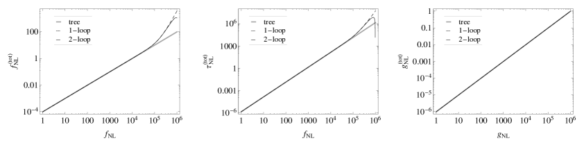
Figure 4: Plot of $f_{\rm NL}^{\rm(tot)}$ (left), $\tau_{\rm NL}^{\rm(tot)}$ (middle) and $g_{\rm NL}^{\rm(tot)}$ (right) as a function of bare non-linear parameters. For other non-linear parameters, we assume the same as in Fig. 1. Here we assume $R=0.01$. However, as long as we set all non-linear parameters to be less than $10^{5}$, we obtain more or less the same results.

Figure 5: Plot of $\tau_{\rm NL}^{\rm(tot)}-(6f_{\rm NL}^{\rm(tot)}/5)^{2}$ (left) and $\tau_{\rm NL}^{\rm(tot)}/(6f_{\rm NL}^{\rm(tot)}/5)^{2}$ (right) for a multi-field model. Here we set non-linear parameters as the same as in Fig. 4. The Suyama-Yamaguchi inequality holds as long as the perturbative expansion is valid.

3.3 Mixed source case II

Next we consider the case where, unlike (17), the curvature perturbation associated with the spectator field $\sigma$ has no linear term so that [19]

$$\zeta=\zeta_{\phi}+\frac{3}{5}f_{\rm NL}\zeta_{\sigma}^{2}+\cdots\,.$$ (25)

The power spectrum in this model is given by

$$P_{\zeta}= P_{\phi}\left\{1+4R\left(\frac{3}{5}\right)^{2}f_{\rm NL}^{2}\left[R{\cal P}_{\phi}(L^{-1})\log(kL)\right]\right.$$

$$\left.\hskip 22.76228pt+\left(\frac{3}{5}\right)^{4}\left\{45g_{\rm NL}^{2}+48f_{\rm NL}h_{\rm NL}\right\}\left[R{\cal P}_{\phi}(L^{-1})\log(kL)\right]^{2}\right\}\,,$$ (26)

where we have again defined $R$ as in (19). However, it should be noted here that $R$ is defined by the ratio of the power spectra of $\sigma$ and $\phi$ at the tree level without including the loop terms. In the case where $\zeta$ is given by Eq. (25), the leading term in the power spectrum of $\sigma$ comes from the loop, thus $R$ does not represent the ratio of the “actual” power spectra which include the loop terms in this case. When the power spectrum is dominated by the loop term from $\sigma$, the primordial fluctuations become highly non-Gaussian, then it is inconsistent with observations, which we will shortly show below. Requiring that the loop term be sub-dominant, we require

$$\left(\frac{5}{6}Rf_{\rm NL}\right)^{2}\mathcal{P}_{\phi}\log(kL)\ll 1.$$ (27)

Thus the combination $Rf_{\rm NL}$ should satisfy

$$Rf_{\rm NL}\ll 10^{5}.$$ (28)

Non-linear parameters in this case are given, up to two-loop order, as

$$f_{\rm NL}^{\rm(tot)}= \frac{5}{6}R^{2}\left\{8\left(\frac{3}{5}\right)^{3}f_{\rm NL}^{3}\left[R~{}{\cal P}_{\phi}(L^{-1})\log(kL)\right]\right.$$

$$\left.+\left(\frac{3}{5}\right)^{5}\left(240f_{\rm NL}^{2}h_{\rm NL}+450f_{\rm NL}g_{\rm NL}^{2}-64Rf_{\rm NL}^{5}\right)\left[R~{}{\cal P}_{\phi}(L^{-1})\log(kL)\right]^{2}\right\},$$ (29)

$$\tau_{\rm NL}^{\rm(tot)}= R^{3}\left\{16\left(\frac{3}{5}\right)^{4}f_{\rm NL}^{4}\left[R~{}{\cal P}_{\phi}(L^{-1})\log(kL)\right]\right.$$

$$\left.+\left(\frac{3}{5}\right)^{6}\left(3672f_{\rm NL}^{2}g_{\rm NL}^{2}+768f_{\rm NL}^{3}h_{\rm NL}-192Rf_{\rm NL}^{6}\right)\left[R~{}{\cal P}_{\phi}(L^{-1})\log(kL)\right]^{2}\right\},$$ (30)

$$g_{\rm NL}^{\rm(tot)}= \frac{R^{3}}{6}\left(\frac{3}{5}\right)^{4}\left(1296f_{\rm NL}^{2}g_{\rm NL}^{2}+576f_{\rm NL}^{3}h_{\rm NL}\right)\left[R~{}{\cal P}_{\phi}(L^{-1})\log(kL)\right]^{2}.$$ (31)

When the condition (28) is not satisfied, $f_{\rm NL}^{\rm(tot)}\gg 10^{5}$, so that the fluctuations are highly non-Gaussian and not allowed by observations.

In Fig. 6, we show $f_{\rm NL}^{\rm(tot)}$, $\tau_{\rm NL}^{\rm(tot)}$, and $g_{\rm NL}^{\rm(tot)}$ as a function of bare non-linear parameters. From the plots of $f_{\rm NL}^{\rm(tot)}$ and $\tau_{\rm NL}^{\rm(tot)}$, one can notice that, for the case with up to two-loop corrections included, the values of the non-linear parameters change their signs from positive to negative at around $f_{\rm NL}\sim 20$, which indicates that the truncation at the two-loop order may be inappropriate beyond this value of $f_{\rm NL}$. Furthermore, interestingly, two-loop terms can dominate over one-loop terms in the small $f_{\rm NL}$ region, as seen from Fig. 6 when we assume relatively large value of $R$. In Fig. 7, we show the dependence of $f_{\rm NL}^{\text{(tot)}}$ on $R$. The two-loop terms contribute to $f_{\rm NL}^{\text{(tot)}}$ appreciably for small values of $f_{\rm NL}$ when $R$ is relatively large. This contribution is coming mainly from $f_{\rm NL}g_{\rm NL}^{2}$ terms, which can be larger than $f_{\rm NL}^{2}h_{\rm NL}$ if $f_{\rm NL}$ is small and $g_{\rm NL}\sim h_{\rm NL}$. Notice that the value for $R$ assumed in the figure satisfies the relation (28): thus, the power spectrum is still dominated by that from $\phi$, which is assumed to be Gaussian here. Since this effect comes from the higher order non-linear parameters such as $g_{\rm NL}$ and $h_{\rm NL}$, we can constrain these parameters from the PLANCK constraints on $f_{\rm NL}^{\rm(tot)}$ and $\tau_{\rm NL}^{\rm(tot)}$, which is shown in Fig. 8, assuming $R=500$ and $f_{\rm NL}=1$. In the figure, shaded regions indicate those satisfying $-8.9<f_{\rm NL}^{\rm(tot)}<14.3$ and $\tau_{\rm NL}^{\rm(tot)}<2800$, which correspond to 95 % constraints from PLANCK. The figure illustrates that, in this kind of model, higher order non-linear parameters can be strongly constrained from those for lower order counterparts. However, we note here that we have included up to the two-loop order terms in this article, and if we include higher order loops such as three loop, the results might be affected. This may be interesting to investigate, but it is beyond the scope of this article and is left for the future work.

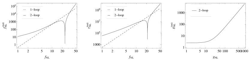
Figure 6: Plot of $f_{\rm NL}^{\rm(tot)}$ (left), $\tau_{\rm NL}^{\rm(tot)}$ (middle) and $g_{\rm NL}^{\rm(tot)}$ (right) as a function of bare non-linear parameters. Here we assume $R=500$. For non-linear parameters, we set $g_{\rm NL}=10^{3}$ for the left and middle panels and $f_{\rm NL}=1$ for the right panel. In all cases, we assume $h_{\rm NL}=10^{3}$.

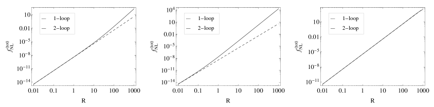
Figure 7: Plot of $f_{\rm NL}^{\rm(tot)}$ as a function of the ratio $R$ for $f_{\rm NL}=1$ and $g_{\rm NL}=10^{3}$ (left), $f_{\rm NL}=1$ and $g_{\rm NL}=10^{4}$ (middle) and $f_{\rm NL}=10$ and $g_{\rm NL}=10^{3}$ (right). We set $h_{\rm NL}=10^{3}$ and other non-linear parameters to vanish for all cases.

Figure 8: PLANCK bounds for $f_{\rm NL}^{\rm(tot)}$ (left) and $\tau_{\rm NL}^{\rm(tot)}$ (right) for $R=500$ and $f_{\rm NL}=1$. The constraint from $\tau_{\rm NL}^{\rm(tot)}$ is stronger than that from $f_{\rm NL}^{\rm(tot)}$.

4 Conclusion and Discussion

We have investigated how higher order non-linear parameters affect the lower order ones through the loop corrections. We have explicitly calculated the corrections for $f_{\rm NL}^{\rm(tot)}$, $\tau_{\rm NL}^{\rm(tot)}$, and $g_{\rm NL}^{\rm(tot)}$ up to two-loop order for single-source and multi-source cases, which have been discussed in the Sections 2 and 3, respectively.

First of all, by explicitly calculating the loop contributions up to two-loop order, we have argued that as long as the bare non-linear parameters are not too large to harm the perturbative expansion of the curvature perturbation, the loop corrections remain very small and the tree contributions are dominant in determining the total observable ones. This is because of the smallness of the loop factor, ${\cal P}_{\zeta}(L^{-1})\log(kL)\sim 2.5\times 10^{-9}$. One may increase the fictitious box size $L$ to have a large logarithmic factor, but then we can no longer resort to the value of the power spectrum ${\cal P}_{\zeta}$ constrained in the observable patch. However, an interesting possibility to avoid this is when the curvature perturbation is sourced by another field, where we have an additional factor $R$. In such a case, the two-loop terms can be important as shown in Fig. 6.

Furthermore, by looking at the expressions of non-linear parameters including loop corrections, we can easily see that, in principle, higher order non-linear parameters can be constrained by the observations of lower order counterparts. Although in general, such a constraint is weak, recent PLANCK results can give a constraint on the bare value of $g_{\rm NL}$ from the constraint on $\tau_{\rm NL}$. Interestingly, the bound for the bare $g_{\rm NL}$ derived from the PLANCK $\tau_{\rm NL}$ constraint $(\tau_{\rm NL}<2800$ at 95 % C.L.) is $g_{\rm NL}\leq 5\times 10^{5}$, which is almost the same as what is directly obtained from trispectrum observations such as WMAP.

In this paper, we have focused on the case of the local type. We note that higher loop corrections can also affect the observables in the non-local form cases.

Now, PLANCK data put a stringent constraint on $f_{\rm NL}$, however, a non-Gaussian signature of primordial density perturbation may come from a higher order one (see Ref. [7] for such an example). In such a case, the results presented in this article should be useful to investigate such a scenario. In addition, when severer constraints on lower order non-linear parameters are obtained in future cosmological observations, we may be able to have more stringent bounds for higher order non-linear parameters from such lower order constraints.

Appendix A Expressions for the power spectrum

The one-loop terms for the power spectrum are

$$P_{\zeta}^{(13)}(k)= 6\left(\frac{3}{5}\right)^{2}g_{\rm NL}P_{\zeta}(k)\left[{\cal P}_{\zeta}(L^{-1})\log(kL)\right]\,,$$ (32)

$$P_{\zeta}^{(22)}(k)= 2\left(\frac{3}{5}\right)^{2}f_{\rm NL}^{2}P_{\zeta}(k)\left[{\cal P}_{\zeta}(L^{-1})\log(kL)\right]\,.$$ (33)

Meanwhile, the two-loop terms are given by

$$P_{\zeta}^{(15)}(k)= 30\left(\frac{3}{5}\right)^{4}i_{\rm NL}P_{\zeta}(k)\left[{\cal P}_{\zeta}(L^{-1})\log(kL)\right]^{2}\,,$$ (34)

$$P_{\zeta}^{(24)}(k)= 48\left(\frac{3}{5}\right)^{4}f_{\rm NL}h_{\rm NL}P_{\zeta}(k)\left[{\cal P}_{\zeta}(L^{-1})\log(kL)\right]^{2}\,,$$ (35)

$$P_{\zeta}^{(33)}(k)= 45\left(\frac{3}{5}\right)^{4}g_{\rm NL}^{2}P_{\zeta}(k)\left[{\cal P}_{\zeta}(L^{-1})\log(kL)\right]^{2}\,.$$ (36)

Appendix B Expressions for the bispectrum

Up to the one-loop corrections to the bispectrum we have

$$B_{\zeta}^{(112)} =\frac{6}{5}f_{\rm NL}\left[P_{\zeta}(k_{1})P_{\zeta}(k_{2})+\text{2 perm}\right]\,,$$ (37)

$$B_{\zeta}^{(222)} =8\left(\frac{3}{5}\right)^{3}f_{\rm NL}^{3}\left[P_{\zeta}(k_{1})P_{\zeta}(k_{2})+\text{2 perm}\right]{\cal P}_{\zeta}(L^{-1})\log(kL)\,,$$ (38)

$$B_{\zeta}^{(123a)} =12\left(\frac{3}{5}\right)^{3}f_{\rm NL}g_{\rm NL}\left[P_{\zeta}(k_{1})P_{\zeta}(k_{2})+\text{2 perm}\right]{\cal P}_{\zeta}(L^{-1})\log(kL)\,,$$ (39)

$$B_{\zeta}^{(123b)} =24\left(\frac{3}{5}\right)^{3}f_{\rm NL}g_{\rm NL}\left[P_{\zeta}(k_{1})P_{\zeta}(k_{2})+\text{2 perm}\right]{\cal P}_{\zeta}(L^{-1})\log(kL)\,,$$ (40)

$$B_{\zeta}^{(114)} =12\left(\frac{3}{5}\right)^{3}h_{\rm NL}\left[P_{\zeta}(k_{1})P_{\zeta}(k_{2})+\text{2 perm}\right]{\cal P}_{\zeta}(L^{-1})\log(kL)\,.$$ (41)

The connected structure of these terms is shown in Fig. 9. Likewise, at the two-loop order the contributions are

$$B^{(116)}_{\zeta}= 90\left(\frac{3}{5}\right)^{5}j_{\rm NL}\left[P_{\zeta}(k_{1})P_{\zeta}(k_{2})+\text{2 perm}\right]\left[{\cal P}_{\zeta}(L^{-1})\log(kL)\right]^{2}\,,$$ (42)

$$B^{(125a)}_{\zeta}= 60\left(\frac{3}{5}\right)^{5}f_{\rm NL}i_{\rm NL}\left[P_{\zeta}(k_{1})P_{\zeta}(k_{2})+\text{2 perm}\right]\left[{\cal P}_{\zeta}(L^{-1})\log(kL)\right]^{2}\,,$$ (43)

$$B^{(125b)}_{\zeta}= 240\left(\frac{3}{5}\right)^{5}f_{\rm NL}i_{\rm NL}\left[P_{\zeta}(k_{1})P_{\zeta}(k_{2})+\text{2 perm}\right]\left[{\cal P}_{\zeta}(L^{-1})\log(kL)\right]^{2}\,,$$ (44)

$$B^{(134a)}_{\zeta}= 144\left(\frac{3}{5}\right)^{5}g_{\rm NL}h_{\rm NL}\left[P_{\zeta}(k_{1})P_{\zeta}(k_{2})+\text{2 perm}\right]\left[{\cal P}_{\zeta}(L^{-1})\log(kL)\right]^{2}\,,$$ (45)

$$B^{(134b)}_{\zeta}= 144\left(\frac{3}{5}\right)^{5}g_{\rm NL}h_{\rm NL}\left[P_{\zeta}(k_{1})P_{\zeta}(k_{2})+\text{2 perm}\right]\left[{\cal P}_{\zeta}(L^{-1})\log(kL)\right]^{2}\,,$$ (46)

$$B^{(134c)}_{\zeta}= 72\left(\frac{3}{5}\right)^{5}g_{\rm NL}h_{\rm NL}\left[P_{\zeta}(k_{1})P_{\zeta}(k_{2})+\text{2 perm}\right]\left[{\cal P}_{\zeta}(L^{-1})\log(kL)\right]^{2}\,,$$ (47)

$$B^{(224a)}_{\zeta}= 144\left(\frac{3}{5}\right)^{5}f_{\rm NL}^{2}h_{\rm NL}\left[P_{\zeta}(k_{1})P_{\zeta}(k_{2})+\text{2 perm}\right]\left[{\cal P}_{\zeta}(L^{-1})\log(kL)\right]^{2}\,,$$ (48)

$$B^{(224b)}_{\zeta}= 96\left(\frac{3}{5}\right)^{5}f_{\rm NL}^{2}h_{\rm NL}\left[P_{\zeta}(k_{1})P_{\zeta}(k_{2})+\text{2 perm}\right]\left[{\cal P}_{\zeta}(L^{-1})\log(kL)\right]^{2}\,,$$ (49)

$$B^{(332a)}_{\zeta}= 360\left(\frac{3}{5}\right)^{5}f_{\rm NL}g_{\rm NL}^{2}\left[P_{\zeta}(k_{1})P_{\zeta}(k_{2})+\text{2 perm}\right]\left[{\cal P}_{\zeta}(L^{-1})\log(kL)\right]^{2}\,,$$ (50)

$$B^{(332b)}_{\zeta}= 18\left(\frac{3}{5}\right)^{5}f_{\rm NL}g_{\rm NL}^{2}\left[P_{\zeta}(k_{1})P_{\zeta}(k_{2})+\text{2 perm}\right]\left[{\cal P}_{\zeta}(L^{-1})\log(kL)\right]^{2}\,,$$ (51)

$$B^{(332c)}_{\zeta}= 72\left(\frac{3}{5}\right)^{5}f_{\rm NL}g_{\rm NL}^{2}\left[P_{\zeta}(k_{1})P_{\zeta}(k_{2})+\text{2 perm}\right]\left[{\cal P}_{\zeta}(L^{-1})\log(kL)\right]^{2}\,,$$ (52)

and the connected structure is as shown in Fig. 10.

Figure 9: Connected structure of the bispectrum up to one-loop corrections.

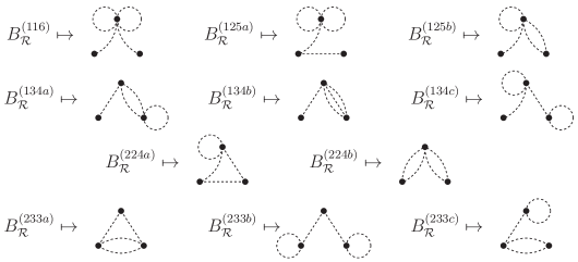
Figure 10: Connected structure of the bispectrum at two-loop order.

Appendix C Expressions for the trispectrum

The two contributions to the tree trispectrum are

$$T_{\zeta}^{(1122)} =2\left(\frac{3}{5}\right)^{2}f_{\rm NL}^{2}\left\{P_{\zeta}(k_{1})P_{\zeta}(k_{2})\left[P_{\zeta}(k_{13})+P_{\zeta}(k_{14})\right]+\text{11 perm}\right\}\,,$$ (53)

$$T_{\zeta}^{(1113)} =\frac{54}{25}g_{\rm NL}\left[P_{\zeta}(k_{1})P_{\zeta}(k_{2})P_{\zeta}(k_{3})+\text{3 perm}\right]\,,$$ (54)

and the one-loop corrections are given by

$$T_{\zeta}^{(2222)} =8\left(\frac{3}{5}\right)^{4}f_{\rm NL}^{4}\left\{P_{\zeta}(k_{1})P_{\zeta}(k_{2})\left[P_{\zeta}(k_{13})+P_{\zeta}(k_{14})\right]+\text{11 perm}\right\}$$

$$\hskip 70.0001pt\times{\cal P}_{\zeta}(L^{-1})\log(kL)\,,$$ (55)

$$T_{\zeta}^{(1223a)} =12\left(\frac{3}{5}\right)^{4}f_{\rm NL}^{2}g_{\rm NL}\left\{P_{\zeta}(k_{1})P_{\zeta}(k_{2})\left[P_{\zeta}(k_{13})+P_{\zeta}(k_{14})\right]+\text{11 perm}\right\}$$

$$\hskip 90.00014pt\times{\cal P}_{\zeta}(L^{-1})\log(kL)\,,$$ (56)

$$T_{\zeta}^{(1223b)} =24\left(\frac{3}{5}\right)^{4}f_{\rm NL}^{2}g_{\rm NL}\left\{P_{\zeta}(k_{1})P_{\zeta}(k_{2})\left[P_{\zeta}(k_{13})+P_{\zeta}(k_{14})\right]+\text{11 perm}\right\}$$

$$\hskip 90.00014pt\times{\cal P}_{\zeta}(L^{-1})\log(kL)\,,$$ (57)

$$T_{\zeta}^{(1223c)} =24\left(\frac{3}{5}\right)^{4}f_{\rm NL}^{2}g_{\rm NL}\Big{(}P_{\zeta}(k_{1})\big{\{}P_{\zeta}(k_{2})P_{\zeta}(k_{3})+\left[P_{\zeta}(k_{2})+P_{\zeta}(k_{3})\right]P_{\zeta}(k_{23})\big{\}}$$

$$\hskip 90.00014pt+\text{11 perm}\Big{)}{\cal P}_{\zeta}(L^{-1})\log(kL)\,,$$ (58)

$$T_{\zeta}^{(1133a)} =54\left(\frac{3}{5}\right)^{4}g_{\rm NL}^{2}\left[P_{\zeta}(k_{1})P_{\zeta}(k_{2})P_{\zeta}(k_{3})+\text{3 perm}\right]{\cal P}_{\zeta}(L^{-1})\log(kL)\,,$$ (59)

$$T_{\zeta}^{(1133b)} =18\left(\frac{3}{5}\right)^{4}g_{\rm NL}^{2}\left\{P_{\zeta}(k_{1})P_{\zeta}(k_{2})\left[P_{\zeta}(k_{13})+P_{\zeta}(k_{14})\right]+\text{11 perm}\right\}$$

$$\hskip 70.0001pt\times{\cal P}_{\zeta}(L^{-1})\log(kL)\,,$$ (60)

$$T_{\zeta}^{(1124a)} =24\left(\frac{3}{5}\right)^{4}f_{\rm NL}h_{\rm NL}\left\{P_{\zeta}(k_{1})P_{\zeta}(k_{2})\left[P_{\zeta}(k_{13})+P_{\zeta}(k_{14})\right]+\text{11 perm}\right\}$$

$$\hskip 90.00014pt\times{\cal P}_{\zeta}(L^{-1})\log(kL)\,,$$ (61)

$$T_{\zeta}^{(1124b)} =144\left(\frac{3}{5}\right)^{4}f_{\rm NL}h_{\rm NL}\left[P_{\zeta}(k_{1})P_{\zeta}(k_{2})P_{\zeta}(k_{3})+\text{3 perm}\right]{\cal P}_{\zeta}(L^{-1})\log(kL)\,,$$ (62)

$$T_{\zeta}^{(1115)} =60\left(\frac{3}{5}\right)^{4}i_{\rm NL}\left[P_{\zeta}(k_{1})P_{\zeta}(k_{2})P_{\zeta}(k_{3})+\text{3 perm}\right]{\cal P}_{\zeta}(L^{-1})\log(kL)\,,$$ (63)

The connected structure of these terms is shown in Fig. 11.

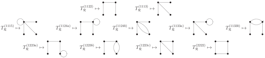
Figure 11: Connected structure of the trispectrum up to one loop.

The terms contributing at the two-loop level are the following:

$$T^{(1117)}_{\zeta}= 630\left(\frac{3}{5}\right)^{6}k_{\rm NL}\left[P_{\zeta}(k_{1})P_{\zeta}(k_{2})P_{\zeta}(k_{3})+\text{3 perm}\right]\left[{\cal P}_{\zeta}(L^{-1})\log(kL)\right]^{2}\,,$$ (64)

$$T_{\zeta}^{(1126a)}= 180\left(\frac{3}{5}\right)^{6}f_{\rm NL}j_{\rm NL}\left\{P_{\zeta}(k_{1})P_{\zeta}(k_{2})\left[P_{\zeta}(k_{13})+P_{\zeta}(k_{14})\right]+\text{11 perm}\right\}\left[{\cal P}_{\zeta}(L^{-1})\log(kL)\right]^{2}\,,$$ (65)

$$T^{(1126b)}_{\zeta}= 2160\left(\frac{3}{5}\right)^{6}f_{\rm NL}j_{\rm NL}\left[P_{\zeta}(k_{1})P_{\zeta}(k_{2})P_{\zeta}(k_{3})+\text{3 perm}\right]\left[{\cal P}_{\zeta}(L^{-1})\log(kL)\right]^{2}\,,$$ (66)

$$T^{(1135a)}_{\zeta}= 270\left(\frac{3}{5}\right)^{6}g_{\rm NL}i_{\rm NL}\left[P_{\zeta}(k_{1})P_{\zeta}(k_{2})P_{\zeta}(k_{3})+\text{3 perm}\right]\left[{\cal P}_{\zeta}(L^{-1})\log(kL)\right]^{2}\,,$$ (67)

$$T_{\zeta}^{(1135b)}= 360\left(\frac{3}{5}\right)^{6}g_{\rm NL}i_{\rm NL}\left\{P_{\zeta}(k_{1})P_{\zeta}(k_{2})\left[P_{\zeta}(k_{13})+P_{\zeta}(k_{14})\right]+\text{11 perm}\right\}\left[{\cal P}_{\zeta}(L^{-1})\log(kL)\right]^{2}\,,$$ (68)

$$T^{(1135c)}_{\zeta}= 540\left(\frac{3}{5}\right)^{6}g_{\rm NL}i_{\rm NL}\left[P_{\zeta}(k_{1})P_{\zeta}(k_{2})P_{\zeta}(k_{3})+\text{3 perm}\right]\left[{\cal P}_{\zeta}(L^{-1})\log(kL)\right]^{2}\,,$$ (69)

$$T^{(1135d)}_{\zeta}= 2160\left(\frac{3}{5}\right)^{6}f_{\rm NL}j_{\rm NL}\left[P_{\zeta}(k_{1})P_{\zeta}(k_{2})P_{\zeta}(k_{3})+\text{3 perm}\right]\left[{\cal P}_{\zeta}(L^{-1})\log(kL)\right]^{2}\,,$$ (70)

$$T_{\zeta}^{(1225a)}= 60\left(\frac{3}{5}\right)^{6}f_{\rm NL}^{2}i_{\rm NL}\left\{P_{\zeta}(k_{1})P_{\zeta}(k_{2})\left[P_{\zeta}(k_{13})+P_{\zeta}(k_{14})\right]+\text{11 perm}\right\}\left[{\cal P}_{\zeta}(L^{-1})\log(kL)\right]^{2}\,,$$ (71)

$$T_{\zeta}^{(1225b)}= 240\left(\frac{3}{5}\right)^{6}f_{\rm NL}^{2}i_{\rm NL}\left\{P_{\zeta}(k_{1})P_{\zeta}(k_{2})\left[P_{\zeta}(k_{13})+P_{\zeta}(k_{14})\right]+\text{11 perm}\right\}\left[{\cal P}_{\zeta}(L^{-1})\log(kL)\right]^{2}\,,$$ (72)

$$T_{\zeta}^{(1225c)}= 720\left(\frac{3}{5}\right)^{6}f_{\rm NL}^{2}i_{\rm NL}\left[P_{\zeta}(k_{1})P_{\zeta}(k_{2})P_{\zeta}(k_{3})+\text{3 perm}\right]\left[{\cal P}_{\zeta}(L^{-1})\log(kL)\right]^{2}$$

$$+240\left(\frac{3}{5}\right)^{6}f_{\rm NL}^{2}i_{\rm NL}\left\{P_{\zeta}(k_{1})P_{\zeta}(k_{2})\left[P_{\zeta}(k_{13})+P_{\zeta}(k_{14})\right]+\text{11 perm}\right\}\left[{\cal P}_{\zeta}(L^{-1})\log(kL)\right]^{2}\,,$$ (73)

$$T_{\zeta}^{(1225d)}= 1440\left(\frac{3}{5}\right)^{6}f_{\rm NL}^{2}i_{\rm NL}\left[P_{\zeta}(k_{1})P_{\zeta}(k_{2})P_{\zeta}(k_{3})+\text{3 perm}\right]\left[{\cal P}_{\zeta}(L^{-1})\log(kL)\right]^{2}$$ (74)

$$T_{\zeta}^{(1144a)}= 864\left(\frac{3}{5}\right)^{6}h_{\rm NL}^{2}\left[P_{\zeta}(k_{1})P_{\zeta}(k_{2})P_{\zeta}(k_{3})+\text{3 perm}\right]\left[{\cal P}_{\zeta}(L^{-1})\log(kL)\right]^{2}$$ (75)

$$T_{\zeta}^{(1144b)}= 72\left(\frac{3}{5}\right)^{6}h_{\rm NL}^{2}\left\{P_{\zeta}(k_{1})P_{\zeta}(k_{2})\left[P_{\zeta}(k_{13})+P_{\zeta}(k_{14})\right]+\text{11 perm}\right\}\left[{\cal P}_{\zeta}(L^{-1})\log(kL)\right]^{2}\,,$$ (76)

$$T_{\zeta}^{(1144c)}= 288\left(\frac{3}{5}\right)^{6}h_{\rm NL}^{2}\left\{P_{\zeta}(k_{1})P_{\zeta}(k_{2})\left[P_{\zeta}(k_{13})+P_{\zeta}(k_{14})\right]+\text{11 perm}\right\}\left[{\cal P}_{\zeta}(L^{-1})\log(kL)\right]^{2}\,,$$ (77)

$$T_{\zeta}^{(1234a)}= 144\left(\frac{3}{5}\right)^{6}f_{\rm NL}g_{\rm NL}h_{\rm NL}\left\{P_{\zeta}(k_{1})P_{\zeta}(k_{2})\left[P_{\zeta}(k_{13})+P_{\zeta}(k_{14})\right]+\text{11 perm}\right\}\left[{\cal P}_{\zeta}(L^{-1})\log(kL)\right]^{2}\,,$$ (78)

$$T_{\zeta}^{(1234b)}= 72\left(\frac{3}{5}\right)^{6}f_{\rm NL}g_{\rm NL}h_{\rm NL}\left\{P_{\zeta}(k_{1})P_{\zeta}(k_{2})\left[P_{\zeta}(k_{13})+P_{\zeta}(k_{14})\right]+\text{11 perm}\right\}\left[{\cal P}_{\zeta}(L^{-1})\log(kL)\right]^{2}\,,$$ (79)

$$T_{\zeta}^{(1234c)}= 288\left(\frac{3}{5}\right)^{6}f_{\rm NL}g_{\rm NL}h_{\rm NL}\left\{P_{\zeta}(k_{1})P_{\zeta}(k_{2})\left[P_{\zeta}(k_{13})+P_{\zeta}(k_{14})\right]+\text{11 perm}\right\}\left[{\cal P}_{\zeta}(L^{-1})\log(kL)\right]^{2}\,,$$ (80)

$$T_{\zeta}^{(1234d)}= 864\left(\frac{3}{5}\right)^{6}f_{\rm NL}g_{\rm NL}h_{\rm NL}\left[P_{\zeta}(k_{1})P_{\zeta}(k_{2})P_{\zeta}(k_{3})+\text{3 perm}\right]\left[{\cal P}_{\zeta}(L^{-1})\log(kL)\right]^{2}$$

$$+288\left(\frac{3}{5}\right)^{6}f_{\rm NL}g_{\rm NL}h_{\rm NL}\left\{P_{\zeta}(k_{1})P_{\zeta}(k_{2})\left[P_{\zeta}(k_{13})+P_{\zeta}(k_{14})\right]+\text{11 perm}\right\}\left[{\cal P}_{\zeta}(L^{-1})\log(kL)\right]^{2}\,,$$ (81)

$$T_{\zeta}^{(1234f)}= 288\left(\frac{3}{5}\right)^{6}f_{\rm NL}g_{\rm NL}h_{\rm NL}\left\{P_{\zeta}(k_{1})P_{\zeta}(k_{2})\left[P_{\zeta}(k_{13})+P_{\zeta}(k_{14})\right]+\text{11 perm}\right\}\left[{\cal P}_{\zeta}(L^{-1})\log(kL)\right]^{2}\,,$$ (82)

$$T_{\zeta}^{(1234g)}= 144\left(\frac{3}{5}\right)^{6}f_{\rm NL}g_{\rm NL}h_{\rm NL}\left\{P_{\zeta}(k_{1})P_{\zeta}(k_{2})\left[P_{\zeta}(k_{13})+P_{\zeta}(k_{14})\right]+\text{11 perm}\right\}\left[{\cal P}_{\zeta}(L^{-1})\log(kL)\right]^{2}\,,$$ (83)

$$T_{\zeta}^{(1234h)}= 72\left(\frac{3}{5}\right)^{6}f_{\rm NL}g_{\rm NL}h_{\rm NL}\left\{P_{\zeta}(k_{1})P_{\zeta}(k_{2})\left[P_{\zeta}(k_{13})+P_{\zeta}(k_{14})\right]+\text{11 perm}\right\}\left[{\cal P}_{\zeta}(L^{-1})\log(kL)\right]^{2}\,,$$ (84)

$$T_{\zeta}^{(1234i)}= 3456\left(\frac{3}{5}\right)^{6}f_{\rm NL}g_{\rm NL}h_{\rm NL}\left[P_{\zeta}(k_{1})P_{\zeta}(k_{2})P_{\zeta}(k_{3})+\text{3 perm}\right]\left[{\cal P}_{\zeta}(L^{-1})\log(kL)\right]^{2}$$

$$+864\left(\frac{3}{5}\right)^{6}f_{\rm NL}g_{\rm NL}h_{\rm NL}\left\{P_{\zeta}(k_{1})P_{\zeta}(k_{2})\left[P_{\zeta}(k_{13})+P_{\zeta}(k_{14})\right]+\text{11 perm}\right\}\left[{\cal P}_{\zeta}(L^{-1})\log(kL)\right]^{2}\,,$$ (85)

$$T_{\zeta}^{(1234l)}= 864\left(\frac{3}{5}\right)^{6}f_{\rm NL}g_{\rm NL}h_{\rm NL}\left[P_{\zeta}(k_{1})P_{\zeta}(k_{2})P_{\zeta}(k_{3})+\text{3 perm}\right]\left[{\cal P}_{\zeta}(L^{-1})\log(kL)\right]^{2}\,,$$ (86)

$$T_{\zeta}^{(4222a)}= 576\left(\frac{3}{5}\right)^{6}f_{\rm NL}^{3}h_{\rm NL}\left[P_{\zeta}(k_{1})P_{\zeta}(k_{2})P_{\zeta}(k_{3})+\text{3 perm}\right]\left[{\cal P}_{\zeta}(L^{-1})\log(kL)\right]^{2}$$

$$+192\left(\frac{3}{5}\right)^{6}f_{\rm NL}^{3}h_{\rm NL}\left\{P_{\zeta}(k_{1})P_{\zeta}(k_{2})\left[P_{\zeta}(k_{13})+P_{\zeta}(k_{14})\right]+\text{11 perm}\right\}\left[{\cal P}_{\zeta}(L^{-1})\log(kL)\right]^{2}\,,$$ (87)

$$T_{\zeta}^{(4222b)}= 192\left(\frac{3}{5}\right)^{6}f_{\rm NL}^{3}h_{\rm NL}\left\{P_{\zeta}(k_{1})P_{\zeta}(k_{2})\left[P_{\zeta}(k_{13})+P_{\zeta}(k_{14})\right]+\text{11 perm}\right\}\left[{\cal P}_{\zeta}(L^{-1})\log(kL)\right]^{2}\,,$$ (88)

$$T_{\zeta}^{(2233a)}= 432\left(\frac{3}{5}\right)^{6}f_{\rm NL}^{2}g_{\rm NL}^{2}\left[P_{\zeta}(k_{1})P_{\zeta}(k_{2})P_{\zeta}(k_{3})+\text{3 perm}\right]\left[{\cal P}_{\zeta}(L^{-1})\log(kL)\right]^{2}$$

$$+144\left(\frac{3}{5}\right)^{6}f_{\rm NL}^{2}g_{\rm NL}^{2}\left\{P_{\zeta}(k_{1})P_{\zeta}(k_{2})\left[P_{\zeta}(k_{13})+P_{\zeta}(k_{14})\right]+\text{11 perm}\right\}\left[{\cal P}_{\zeta}(L^{-1})\log(kL)\right]^{2}\,,$$ (89)

$$T_{\zeta}^{(2233b)}= 1008\left(\frac{3}{5}\right)^{6}f_{\rm NL}^{2}g_{\rm NL}^{2}\left\{P_{\zeta}(k_{1})P_{\zeta}(k_{2})\left[P_{\zeta}(k_{13})+P_{\zeta}(k_{14})\right]+\text{11 perm}\right\}\left[{\cal P}_{\zeta}(L^{-1})\log(kL)\right]^{2}\,,$$ (90)

$$T_{\zeta}^{(2233c)}= 36\left(\frac{3}{5}\right)^{6}f_{\rm NL}^{2}g_{\rm NL}^{2}\left\{P_{\zeta}(k_{1})P_{\zeta}(k_{2})\left[P_{\zeta}(k_{13})+P_{\zeta}(k_{14})\right]+\text{11 perm}\right\}\left[{\cal P}_{\zeta}(L^{-1})\log(kL)\right]^{2}\,,$$ (91)

$$T_{\zeta}^{(2233d)}= 72\left(\frac{3}{5}\right)^{6}f_{\rm NL}^{2}g_{\rm NL}^{2}\left\{P_{\zeta}(k_{1})P_{\zeta}(k_{2})\left[P_{\zeta}(k_{13})+P_{\zeta}(k_{14})\right]+\text{11 perm}\right\}\left[{\cal P}_{\zeta}(L^{-1})\log(kL)\right]^{2}\,,$$ (92)

$$T_{\zeta}^{(2233e)}= 864\left(\frac{3}{5}\right)^{6}f_{\rm NL}^{2}g_{\rm NL}^{2}\left[P_{\zeta}(k_{1})P_{\zeta}(k_{2})P_{\zeta}(k_{3})+\text{3 perm}\right]\left[{\cal P}_{\zeta}(L^{-1})\log(kL)\right]^{2}$$

$$+432\left(\frac{3}{5}\right)^{6}f_{\rm NL}^{2}g_{\rm NL}^{2}\left\{P_{\zeta}(k_{1})P_{\zeta}(k_{2})\left[P_{\zeta}(k_{13})+P_{\zeta}(k_{14})\right]+\text{11 perm}\right\}\left[{\cal P}_{\zeta}(L^{-1})\log(kL)\right]^{2}\,,$$ (93)

$$T_{\zeta}^{(2233g)}= 144\left(\frac{3}{5}\right)^{6}f_{\rm NL}^{2}g_{\rm NL}^{2}\left\{P_{\zeta}(k_{1})P_{\zeta}(k_{2})\left[P_{\zeta}(k_{13})+P_{\zeta}(k_{14})\right]+\text{11 perm}\right\}\left[{\cal P}_{\zeta}(L^{-1})\log(kL)\right]^{2}\,,$$ (94)

$$T_{\zeta}^{(1333a)}= 108\left(\frac{3}{5}\right)^{6}g_{\rm NL}^{3}\left\{P_{\zeta}(k_{1})P_{\zeta}(k_{2})\left[P_{\zeta}(k_{13})+P_{\zeta}(k_{14})\right]+\text{11 perm}\right\}\left[{\cal P}_{\zeta}(L^{-1})\log(kL)\right]^{2}\,,$$ (95)

$$T_{\zeta}^{(1333b)}= 162\left(\frac{3}{5}\right)^{6}g_{\rm NL}^{3}\left[P_{\zeta}(k_{1})P_{\zeta}(k_{2})P_{\zeta}(k_{3})+\text{3 perm}\right]\left[{\cal P}_{\zeta}(L^{-1})\log(kL)\right]^{2}\,,$$ (96)

$$T_{\zeta}^{(1333c)}= 648\left(\frac{3}{5}\right)^{6}g_{\rm NL}^{3}\left[P_{\zeta}(k_{1})P_{\zeta}(k_{2})P_{\zeta}(k_{3})+\text{3 perm}\right]\left[{\cal P}_{\zeta}(L^{-1})\log(kL)\right]^{2}$$

$$+216\left(\frac{3}{5}\right)^{6}g_{\rm NL}^{3}\left\{P_{\zeta}(k_{1})P_{\zeta}(k_{2})\left[P_{\zeta}(k_{13})+P_{\zeta}(k_{14})\right]+\text{11 perm}\right\}\left[{\cal P}_{\zeta}(L^{-1})\log(kL)\right]^{2}\,.$$ (97)

For the connected structure, see Fig. 12.

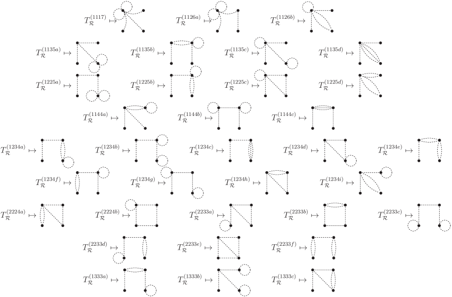
Figure 12: Connected structure of the trispectrum at two-loop order.

References

- [1] P. A. R. Ade et al. [Planck Collaboration], arXiv:1303.5082 [astro-ph.CO].
- [2] P. A. R. Ade et al. [Planck Collaboration], arXiv:1303.5084 [astro-ph.CO].
- [3] T. Sekiguchi and N. Sugiyama, JCAP 1309, 002 (2013) [arXiv:1303.4626 [astro-ph.CO]].
- [4] V. Desjacques and U. Seljak, Phys. Rev. D 81, 023006 (2010) [arXiv:0907.2257 [astro-ph.CO]] ; J. Smidt, A. Amblard, C. T. Byrnes, A. Cooray, A. Heavens and D. Munshi, Phys. Rev. D 81, 123007 (2010) [arXiv:1004.1409 [astro-ph.CO]] ; D. M. Regan, E. P. S. Shellard and J. R. Fergusson, Phys. Rev. D 82, 023520 (2010) [arXiv:1004.2915 [astro-ph.CO]] ; T. Giannantonio, A. J. Ross, W. J. Percival, R. Crittenden, D. Bacher, M. Kilbinger, R. Nichol and J. Weller, arXiv:1303.1349 [astro-ph.CO].
- [5] K. Enqvist and M. S. Sloth, Nucl. Phys. B 626, 395 (2002) [arXiv:hep-ph/0109214] ; D. H. Lyth and D. Wands, Phys. Lett. B 524, 5 (2002) [arXiv:hep-ph/0110002] ; T. Moroi and T. Takahashi, Phys. Lett. B 522, 215 (2001) [Erratum-ibid. B 539, 303 (2002)] [arXiv:hep-ph/0110096].
- [6] G. Dvali, A. Gruzinov, M. Zaldarriaga, Phys. Rev. D69, 023505 (2004) [astro-ph/0303591] ; L. Kofman, [astro-ph/0303614].
- [7] T. Suyama, T. Takahashi, M. Yamaguchi and S. Yokoyama, JCAP 1306, 012 (2013) [arXiv:1303.5374 [astro-ph.CO]].
- [8] D. H. Lyth, Phys. Rev. D 45, 3394 (1992).
- [9] C. T. Byrnes, S. Nurmi, G. Tasinato and D. Wands, Europhys. Lett. 103, 19001 (2013) [arXiv:1306.2370 [astro-ph.CO]].
- [10] E. D. Stewart, Phys. Rev. D 65, 103508 (2002) [astro-ph/0110322] ; J. Choe, J. -O. Gong and E. D. Stewart, JCAP 0407, 012 (2004) [hep-ph/0405155].
- [11] J. -O. Gong, H. Noh and J. -c. Hwang, JCAP 1104, 004 (2011) [arXiv:1011.2572 [astro-ph.CO]].
- [12] G. Tasinato, C. T. Byrnes, S. Nurmi and D. Wands, Phys. Rev. D 87, 043512 (2013) [arXiv:1207.1772 [hep-th]].
- [13] J. Smidt, A. Amblard, C. T. Byrnes, A. Cooray, A. Heavens and D. Munshi, in Ref. [4].
- [14] D. Langlois and F. Vernizzi, Phys. Rev. D 70, 063522 (2004) [arXiv:astro-ph/0403258] ; T. Moroi, T. Takahashi and Y. Toyoda, Phys. Rev. D 72, 023502 (2005) [arXiv:hep-ph/0501007] ; T. Moroi and T. Takahashi, Phys. Rev. D 72, 023505 (2005) [arXiv:astro-ph/0505339] ; K. Ichikawa, T. Suyama, T. Takahashi and M. Yamaguchi, Phys. Rev. D 78, 023513 (2008) [arXiv:0802.4138 [astro-ph]] ; T. Suyama, T. Takahashi, M. Yamaguchi and S. Yokoyama, JCAP 1012, 030 (2010) [arXiv:1009.1979 [astro-ph.CO]].
- [15] K. Ichikawa, T. Suyama, T. Takahashi and M. Yamaguchi, Phys. Rev. D 78, 063545 (2008) [arXiv:0807.3988 [astro-ph]].
- [16] K. Enqvist and T. Takahashi, JCAP 1310, 034 (2013) [arXiv:1306.5958 [astro-ph.CO]].
- [17] T. Suyama and M. Yamaguchi, Phys. Rev. D 77, 023505 (2008) [arXiv:0709.2545 [astro-ph]].
- [18] N. S. Sugiyama, JCAP 1205, 032 (2012) [arXiv:1201.4048 [gr-qc]].
- [19] L. Boubekeur and D. .H. Lyth, Phys. Rev. D 73, 021301 (2006) [astro-ph/0504046] ; T. Suyama and F. Takahashi, JCAP 0809, 007 (2008) [arXiv:0804.0425 [astro-ph]].