On the Jones Polynomial of $2n$-plat presentations of knots

Abstract.

In this paper, a method is given to calculate the Jones polynomial of the 6-plat presentations of knots by using a representation of the braid group $\mathbb{B}_{6}$ into a group of $5\times 5$ matrices. We also can calculate the Jones polynomial of the $2n$-plat presentations of knots by generalizing the method for the $6$-plat presentations of knots.

1. Introduction

In 1985, Jones [8] discovered the polynomial knot invariant $V_{K}(t)$ and gave a formula to calculate the polynomials of knots that are presented as closed braids. He also gave a formula to calculate the Jones polynomials of knots that are presented as closed plats. The closed plat formula is described in [3]. Birman and Kanenobu [3] generalized the formula to the polynomials of knots which are obtained by a combination of closed braid and plat. In the case of $2n$-plat, by using the skein relation of Jones polynomial, we have $2^{n}$ closed braids that is related to the given $2n$-plat. Then the Jones polynomial of the $2n$-plat can be obtained from the Jones polynomials of the $2^{n}$ closed braids.

Kauffman [9] introduced the Kauffman bracket $<K>$ and the writhe $w(K)$ to calculate the Kauffman polynomial $X_{K}(a)$, which is identical to the Jones polynomial $V_{K}(t)$ with the change of variable $t=a^{4}$.

In this paper, by using the skein relation of the Kauffman bracket, we present a method to calculate the Kauffman bracket and the writhe of 6-plat presentaions of knots that is obtained directly from the $6$-plat presentation. Also, we indicate how it extends to $2n$-plat presentations of knots.

Let $S^{2}$ be a sphere smoothly embedded in $S^{3}$ and let $K$ be a knot transverse to $S^{2}$. The complement in $S^{3}$ of $S^{2}$ consists of two open balls, $B_{1}$ and $B_{2}$. We assume that $S^{2}$ is the $xz$-plane $\cup~{}\{\infty\}$. Let $p$ be the projection onto the $xy$-plane from $\mathbb{R}^{3}$. Then the projection of $S^{2}-\{\infty\}$ onto the $xy$-plane is the $x$-axis, and $B_{1}$ projects to the upper half plane. Similarly, $B_{2}$ projects to the lower half plane. The resulting diagram of $K$ is called a plat on $2n$-strings, denoted by $p_{2n}(w)$, if it is the union of a $2n$-braid $w$ and $2n$ unlinked and unknotted arcs which connect pairs of consecutive strings of the braid at the top and at the bottom endpoints and $S^{2}$ meets the top of the $2n$-braid. The bridge (plat) number $b(K)$ of $K$ is the smallest possible number $n$ such that there exists a plat presentation of $K$ on $2n$ strings. We remark that the braid group $\mathbb{B}_{2n}$ is generated by $\sigma_{1},\sigma_{2},\cdot\cdot\cdot\sigma_{2n-1}$ which are twistings of two adjacent strings. For example, $w=\sigma_{2}^{-1}\sigma_{4}^{-1}\sigma_{3}\sigma_{1}^{3}\sigma_{5}^{2}\sigma_{4}^{-1}\sigma_{2}^{-1}$ is the word for the 6 braid in the dotted rectangle of the first diagram of Figure 1.

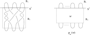
Figure 1.

Then we say that a plat presentation is standard if the $2n$-braid $w$ of $p_{2n}(w)$ involves only $\sigma_{2},\sigma_{3},\cdot\cdot\cdot,\sigma_{2n-1}$.

Let $q_{2n}(w)=p_{2n}(w)\cap B_{2}$ be the plat presentation for the rational $n$-tangles $K\cap B_{2}$. [See [6].]

We say that $\overline{q_{2n}(w)}=p_{2n}(w)$ is the plat closure of $q_{2n}(w)$.

The tangle diagrams with the circles in Figure 3 give the diagrams of trivial rational $2,3$-tangles as in $[1],[4],[7],[10]$. The right side of the diagrams show the trivial rational $2,3$-tangles in $B_{2}$.

We note that $q_{2n}(w)$ is alternating if and only if $\overline{q_{2n}(w)}$ is alternating.

A tangle $T$ is reduced alternating if $T$ is alternating and $T$ does not have a self-crossing which can be removed by a Type I Reidemeister move. (See [1].) We say that a knot $K$ is in n-bridge position if the projection of $K$ onto the $xy$-plane has a plat presentation $p_{2n}(w)$.

Figure 2.

Let $\Lambda=\mathbb{Z}[a,a^{-1}]$ and $L$ be a link.

We recall that the Kauffman bracket $<L>\in\Lambda$ of a link $L$ is obtained from the following three axioms (See [1].)

The symbol $<~{}>$ indicates that the changes are made to the diagram locally, while the rest of the diagram is fixed.

The Kauffman polynomial $X_{L}(a)\in\Lambda$ is defined by

$X_{L}(a)=(-a^{-3})^{w(\overrightarrow{L})}<L>$,

where the writhe $w(\overrightarrow{L})\in\mathbb{Z}$ is obtained by assigning an orientation to $L$, and taking a sum over all crossings of $L$ of their indices $e$, which are given by the following rule

In section 2, we introduce a theorem that explains how to calculate the Kauffman brackets for 4-plat presentations of knots.

In section 3, we show the main theorem that gives us a formula to calculate the Kauffman brackets for 6-plat presentations of knots.

In section 4, we generalize the formulas given in sections 3 to the Kauffman brackets of $2n$-plat presentations of knots.

Then, we give a method to calculate the writhes of of $n$-bridge presentations in section 5.

The author would like to thank his advisor Dr. Myers for his consistent encouragement and sharing his enlightening ideas on this topic.

2. The Kauffman brackets of the 4-plat presentations of knots

For given 2-tangles $T$ and $U$, we denote by $T+U$ the tangle sum of $T,~{}U$ and by $T*U$ the “vertical sum” of $T,~{}U$ as in Figure 4.

Figure 3. the tangles 0,$\infty$, 1 and the tangle combinations $T+U,~{}T*U$.

Goldman and Kauffman [6] define the bracket polynomial of the rational 2-tangle diagram $T$ as $<T>=f^{T}(a)<0>+g^{T}(a)<{\infty}>$, where the coefficients $f^{T}(a)$ and $g^{T}(a)$ are Laurent polynomials that are obtained by starting with $T$ and using the three axioms repeatedly until only the two trivial tangles $T_{0}$ and $T_{\infty}$ in the expression given for $T$ are left. Then we define the bracket vector of $T$ to be the ordered pair $[f^{T}(a),g^{T}(a)]^{t}$, and denote it by $br(T)$. For example, $br(1)=[a^{-1},a]^{t}$, where $1$ is the rational 2-tangle with only one positive crossing.

Eliahou-Kauffman-Thistlethwaite [5] established the following.

Proposition 2.1.

For given 2-tangles $T$ and $U$, and $k=-a^{2}-a^{-2}$,

$br(T+U)=\left[\begin{array}[]{cc}f^{U}(a)&0\\ g^{U}(a)&f^{U}(a)+kg^{U}(a)\\ \end{array}\right]br(T)$ and, $br(T\ast U)=\left[\begin{array}[]{cc}kf^{U}(a)+g^{U}(a)&f^{U}(a)\\ 0&g^{U}(a)\\ \end{array}\right]br(T).$

So, if $U=1$ in Proposition 2.1 then we have the following equalities.

$br(T+1)=M_{+}\cdot br(T)$, $br(T*1)=M_{*}\cdot br(T)$, where

$M_{+}=\left[\begin{array}[]{cc}a^{-1}&0\\ a&-a^{3}\\ \end{array}\right]$ and $M_{*}=\left[\begin{array}[]{cc}-a^{-3}&a^{-1}\\ 0&a\\ \end{array}\right].$

Two rational $2$-tangles, $T,T^{\prime}$, in $B^{3}$ are isotopic, denoted by $T\sim T^{\prime}$, if there is an orientation-preserving self-homeomorphism $h:(B^{3},T)\rightarrow(B^{3},T^{\prime})$ that is the identity map on the boundary.

We say that $T^{hflip}$ is the horizontal flip of the 2-tangle $T$ if $T^{hflip}$ is obtained from $T$ by a $180^{\circ}$-rotation around a horizontal axis on the plane of $T$, and $T^{vflip}$ is the vertical flip of the tangle $T$ if $T^{vflip}$ is obtained from $T$ by a $180^{\circ}$-rotation around a vertical axis, see Figure 5 for illustrations. Then we have the following lemma by Kauffman.

Lemma 2.2.

$($Flipping Lemma $[7])$ If $T$ is rational 2-tangle, then $T\sim T^{vflip}$ and $T\sim T^{hflip}$.

We note that any rational 2-tangle $T$ can be obtained from an element $u$ of the braid group $\mathbb{B}_{3}$ as in the first bottom diagram of Figure 5. (Refer to [7].)

For $u=\sigma_{k_{1}}^{\epsilon_{1}}\sigma_{k_{2}}^{\epsilon_{2}}\cdot\cdot\cdot\sigma_{k_{n}}^{\epsilon_{n}}$, the reverse word of $u$, denoted by $u^{r}$, is defined by the word $u^{r}=\sigma_{k_{n}}^{\epsilon_{n}}\sigma_{k_{n-1}}^{\epsilon_{n-1}}\cdot\cdot\cdot\sigma_{k_{1}}^{\epsilon_{1}}$. Then by Lemma 2.2, we see how to get a word $u^{r}$ for a 4-plat presentation of a rational 2-tangle $T$ as in the bottom diagrams of Figure 5.

Figure 4.

Suppose that $R$ is a rational 2-tangle. Let $u$ be the word for a standard 4-plat presentation of $R$. Then, by modifying the diagrams of $R+1$ and $R\ast 1$ as in Figure 6, we see that $u^{\prime}=\sigma_{3}^{-1}w$ and $u^{\prime\prime}=\sigma_{2}w$, where $u^{\prime}$ and $u^{\prime\prime}$ are the words for 4-plat presentations of $R+1$ and $R\ast 1$ respectively.

Figure 5.

Now, consider the following theorem.

Theorem 2.3.

$[$Conway$,($See$~{}[10])]$ If $K$ is a 2-bridge knot, then there exists a word $w$ in $\mathbb{B}_{4}$ so that the plat presentation $p_{4}(w)$ is reduced alternating and standard and represents a knot isotopic to $K$.

Let $A_{2}=M_{*}$ and $A_{3}=M_{+}^{-1}$.

Then we can derive the following theorem which shows how to calculate the Jones polynomials of 4-plat presentations of knots.

Theorem 2.4.

Suppose that $q_{4}(w)$ is a plat presentation of a rational 2-tangle $T$ which is reduced alternating and standard so that $w=\sigma_{3}^{-\epsilon_{1}}\sigma_{2}^{\epsilon_{2}}\cdot\cdot\cdot\sigma_{3}^{-\epsilon_{2n-1}}\sigma_{2}^{\epsilon_{2n}}$ for some positive integers $\epsilon_{i}$ ($2\leq i\leq 2n$) and non-negative integer $\epsilon_{1}$. Let $A=A_{3}^{-\epsilon_{1}}A_{2}^{\epsilon_{2}}\cdot\cdot\cdot A_{3}^{-\epsilon_{2n-1}}A_{2}^{\epsilon_{2n}}$. Then,

$<T>=f^{T}(a)<T_{0}>+g^{T}(a)<T_{\infty}>$, where $f^{T}(a)$ and $g^{T}(a)$ are given by $br(T)=[f^{T}(a),g^{T}(a)]^{t}=A[0,1]^{t}$ and $<K>=f^{T}(a)-(a^{2}+a^{-2})g^{T}(a)$ for $K$, where $K$ is represented by the plat presentation $\overline{q_{4}(w)}$.

Therefore, $X_{K}=(-a^{-3})^{w({K})}(f^{T}(a)-(a^{2}+a^{-2})g^{T}(a))$, where $w(K)$ is the writhe of the knot $K$.

Proof.

Let $l=|\epsilon_{1}|+|\epsilon_{2}|+\cdot\cdot\cdot+|\epsilon_{2n}|$.

We will show this theorem by using induction on $l$.

Suppose that $w=\sigma_{2}$. Then $T=\infty\ast 1$.

Therefore, by Proposition 2.1., $br(T)=M_{*}[0,1]^{t}=A_{2}[0,1]^{t}$.

Now, we assume that $br(T)=[f^{T}(a),g^{T}(a)]^{t}=A[0,1]^{t}$ if $T$ is a reduced alternating standard rational 2-tangle with the plat presentation $q_{4}(w)$, where $w=\sigma_{3}^{-\epsilon_{1}}\sigma_{2}^{\epsilon_{2}}\cdot\cdot\cdot\sigma_{2}^{\epsilon_{2n}}$ for some positive integers $\epsilon_{i}$ ($2\leq i\leq 2n$) and non-negative integer $\epsilon_{1}$, and $l=|\epsilon_{1}|+|\epsilon_{2}|+\cdot\cdot\cdot+|\epsilon_{2n}|=k$.

Now, consider a reduced alternating standard rationl 2-tangle $T^{\prime}$ with the plat presentation $q_{4}(w^{\prime})$, where $w^{\prime}=\sigma_{3}^{-\epsilon_{1}^{\prime}}\sigma_{2}^{\epsilon_{2}^{\prime}}\cdot\cdot\cdot\sigma_{2}^{\epsilon_{2m}^{\prime}}$ for some positive integers $\epsilon_{i}$ ($2\leq i\leq 2m$) and non-negative integer $\epsilon_{1}^{\prime}$, and $l=|\epsilon_{1}^{\prime}|+|\epsilon_{2}^{\prime}|+\cdot\cdot\cdot+|\epsilon_{2m}^{\prime}|=k+1$.

If $\epsilon_{i}^{\prime}\geq 1$ then we set $w^{\prime\prime}=\sigma_{3}^{-(\epsilon_{1}^{\prime}-1)}\sigma_{2}^{\epsilon_{2}^{\prime}}\cdot\cdot\cdot\sigma_{2}^{\epsilon_{2m}^{\prime}}$. Then $w^{\prime}=\sigma_{3}^{-1}w^{\prime\prime}$.

Let $T^{\prime\prime}$ be the reduced alternating standard rational 2-tangle with the plat presentation $q_{4}(w^{\prime\prime})$.

Let $A^{\prime}=A_{3}^{-\epsilon_{1}^{\prime}}A_{2}^{\epsilon_{2}^{\prime}}\cdot\cdot\cdot A_{2}^{\epsilon_{2m}^{\prime}}$ and $A^{\prime\prime}=A_{3}^{-(\epsilon_{1}^{\prime}-1)}A_{2}^{\epsilon_{2}^{\prime}-1}\cdot\cdot\cdot A_{2}^{\epsilon_{2m}^{\prime}}$.

Since $|\epsilon_{1}^{\prime}-1|+|\epsilon_{2}^{\prime}|+\cdot\cdot\cdot+|\epsilon_{2m}^{\prime}|=k$, we note that $br(T^{\prime\prime})=[f^{T^{\prime\prime}}(a),g^{T^{\prime\prime}}(a)]^{t}=A^{\prime\prime}[0,1]^{t}$ by assumption. We note that $T^{\prime}=T^{\prime\prime}+1$. So, by Proposition 2.1., $br(T^{\prime})=M_{+}\cdot br(T^{\prime\prime})=A_{3}^{-1}(A^{\prime\prime}[0,1]^{t})=(A_{3}^{-1}A^{\prime\prime})[0,1]^{t}=A^{\prime}[0,1]^{t}$.

If $\epsilon_{1}^{\prime}=0$ then we set $w^{\prime\prime}=\sigma_{2}^{\epsilon_{2}^{\prime}-1}\cdot\cdot\cdot\sigma_{2}^{\epsilon_{2m}^{\prime}}$. Then $w^{\prime}=\sigma_{2}w^{\prime\prime}$.

Let $T^{\prime\prime}$ be the reduced alternating standard rational 2-tangle with the plat presentation $q_{4}(w^{\prime\prime})$.
Let $A^{\prime}=A_{2}^{\epsilon_{2}^{\prime}}\cdot\cdot\cdot A_{2}^{\epsilon_{2m}^{\prime}}$ and $A^{\prime\prime}=A_{2}^{\epsilon_{2}^{\prime}-1}\cdot\cdot\cdot A_{2}^{\epsilon_{2m}^{\prime}}$.

Since $|\epsilon_{2}^{\prime}-1|+\cdot\cdot\cdot+|\epsilon_{2m}^{\prime}|=k$, we note that $br(T^{\prime\prime})=[f^{T^{\prime\prime}}(a),g^{T^{\prime\prime}}(a)]^{t}=A^{\prime\prime}[0,1]^{t}$ by assumption.
We note that $T^{\prime}=T^{\prime\prime}\ast 1$. So, by Proposition 2.1., $br(T^{\prime})=M_{*}\cdot br(T^{\prime\prime})=A_{2}(A^{\prime\prime}[0,1]^{t})=(A_{2}A^{\prime\prime})[0,1]^{t}=A^{\prime}[0,1]^{t}$. ∎

Now, assume that $q_{4}(w)$ be a 4-plat presentation of a rational 2-tangle $T$ which is reduced alternating and standard so that $w=\sigma_{3}^{-\epsilon_{1}}\sigma_{2}^{\epsilon_{2}}\cdot\cdot\cdot\sigma_{3}^{-\epsilon_{2n-1}}\sigma_{2}^{\epsilon_{n}}$ for some negative integers $\epsilon_{i}$ ($2\leq i\leq 2n$) and non-positive integer $\epsilon_{1}$.

We can calculate the Kauffman bracket of $q_{4}((w^{-1})^{r})$ by usinge the previous theorem.

We note that $q_{4}(w)$ is the mirror image of $q_{4}((w^{-1})^{r})$ which is obtained by interchanging the over and under crossings.

So, we switch $a$ and $a^{-1}$ to calculate the Kauffman bracket of the 4-plat presentation $q_{4}(w)$ of the rational 2-tangle $T$.

3. The Kauffman brackets of the 6-plat presentations of knots

Now, suppose that $K$ is in 3-bridge position. Then we have a plat presentation $q_{6}(w)$ for the rational 3-tangle $K\cap B_{2}$. Then, let $w=\sigma_{k_{1}}^{\epsilon_{1}}\sigma_{k_{2}}^{\epsilon_{2}}\cdot\cdot\cdot\sigma_{k_{n-1}}^{\epsilon_{n-1}}\sigma_{k_{n}}^{\epsilon_{n}}$ for some non-zero integers $\epsilon_{i}$ ($1\leq i\leq n$), where $k_{i}\in\{1,2,3,4,5\}$.

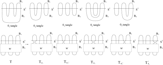
Figure 6.

H. Cabrera-Ibarra [4] defined the bracket polynomial of the rational 3-tangle $T$ as $<T>=f^{T}_{1}(a)<{0_{1}}>+f^{T}_{2}(a)<{0_{2}}>+f^{T}_{3}(a)<{0_{3}}>+f^{T}_{4}(a)<{0_{4}}>+f^{T}_{5}<{0_{5}}>$, where $f^{T}_{i}(a)$ are polynomials in $a$ and $a^{-1}$ that are obtained by starting with $T$ and using the three axioms repeatedly until only the five trivial tangles $<{0_{j}}>$ in the expression given for $T$ are left. (See Figure 6 and 7.)

Let $\mathcal{A}=<{0_{1}}>,\mathcal{B}=<{0_{2}}>,\mathcal{C}=<{0_{3}}>,\mathcal{D}=<{0_{4}}>$ and $\mathcal{E}=<{0_{5}}>$.

Let $B_{1}^{\pm 1}=\left[\begin{array}[]{ccccc}a^{\pm 1}&0&0&0&0\\ 0&a^{\pm 1}&0&0&0\\ 0&a^{\mp 1}&-a^{\mp 3}&a^{\mp 1}&0\\ 0&0&0&a^{\pm 1}&0\\ a^{\mp 1}&0&0&0&-a^{\mp 3}\\ \end{array}\right],$       $B_{2}^{\pm 1}=\left[\begin{array}[]{ccccc}-a^{\mp 3}&0&0&a^{\mp 1}&a^{\mp 1}\\ 0&-a^{\mp 3}&a^{\mp 1}&0&0\\ 0&0&a^{\pm 1}&0&0\\ 0&0&0&a^{\pm 1}&0\\ 0&0&0&0&a^{\pm 1}\\ \end{array}\right]$,

$~{}\hskip 18.0ptB_{3}^{\pm 1}=\left[\begin{array}[]{ccccc}a^{\pm 1}&0&0&0&0\\ 0&a^{\pm 1}&0&0&0\\ 0&a^{\mp 1}&-a^{\mp 3}&0&a^{\mp 1}\\ a^{\mp 1}&0&0&-a^{\mp 3}&0\\ 0&0&0&0&a^{\pm 1}\\ \end{array}\right]$,       $B_{4}^{\pm 1}=\left[\begin{array}[]{ccccc}-a^{\mp 3}&a^{\mp 1}&0&a^{\mp 1}&0\\ 0&a^{\pm 1}&0&0&0\\ 0&0&a^{\pm 1}&0&0\\ 0&0&0&a^{\pm 1}&0\\ 0&0&a^{\mp 1}&0&-a^{\mp 3}\\ \end{array}\right],\\$

$~{}\hskip 18.0ptB_{5}^{\pm 1}=\left[\begin{array}[]{ccccc}a^{\pm 1}&0&0&0&0\\ a^{\mp 1}&-a^{\mp 3}&0&0&0\\ 0&0&-a^{\mp 3}&a^{\mp 1}&a^{\mp 1}\\ 0&0&0&a^{\pm 1}&0\\ 0&0&0&0&a^{\pm 1}\\ \end{array}\right].$

Let $B=B_{k_{1}}^{\epsilon_{1}}B_{k_{2}}^{\epsilon_{2}}\cdot\cdot\cdot B_{k_{n-1}}^{\epsilon_{n-1}}B_{k_{n}}^{\epsilon_{n}}$.

Then we have the following theorem to calculate the Kauffman polynomial of $K$.

Theorem 3.1.

Suppose that $q_{6}(w)$ is a plat presentation for a rational 3-tangle $T$ and $w=\sigma_{k_{1}}^{\epsilon_{1}}\sigma_{k_{2}}^{\epsilon_{2}}\cdot\cdot\cdot\sigma_{k_{n-1}}^{\epsilon_{n-1}}\sigma_{k_{n}}^{\epsilon_{n}}$ for some non-zero integers $\epsilon_{i}$ ($1\leq i\leq n$), where $k_{i}\in\{1,2,3,4,5\}$.

Then $<T>=f^{T}_{1}(a)\mathcal{A}+f^{T}_{2}(a)\mathcal{B}+f^{T}_{3}(a)\mathcal{C}+f^{T}_{4}(a)\mathcal{D}+f^{T}_{5}(a)\mathcal{E}$ , where $f^{T}_{i}(a)$ are given by

$[f^{T}_{1}(a)~{}f^{T}_{2}(a)~{}f^{T}_{3}(a)~{}f^{T}_{4}(a)~{}f^{T}_{5}(a)]^{t}=B[0~{}0~{}1~{}0~{}0]^{r},$ and $B=B_{k_{1}}^{\epsilon_{1}}B_{k_{2}}^{\epsilon_{2}}\cdot\cdot\cdot B_{k_{n-1}}^{\epsilon_{n-1}}B_{k_{n}}^{\epsilon_{n}}$. (i.e., the third column of $B$)

Also, $<K>=f^{T}_{1}(a)+k(f^{T}_{2}(a)+f^{T}_{4}(a)+f^{T}_{5}(a))+k^{2}f^{T}_{3}(a)$, where $k=-a^{2}-a^{-2}$ and $K$ is the knot which is represented by the plat presentation $\overline{q_{6}(w)}$.

Therefore, $X_{K}=(-a^{-3})^{w(\overrightarrow{K})}(f^{T}_{1}(a)+k(f^{T}_{2}(a)+f^{T}_{4}(a)+f^{T}_{5}(a))+k^{2}f^{T}_{3}(a))$.

Proof.

Suppose that $K$ is a 3-bridge link. Then, we have a link $K^{\prime}$ which is isotopic to $K$ and the projection onto the $xy$-plane has a plat presentation $p_{6}(w)$. Then we define $q_{6}(w)$ that is the plat presentation of the tangle $T=K^{\prime}\cap B_{2}$ as in the first bottom diagram of Figure 6.

Suppose that $<T>=f^{T}_{1}(a)\mathcal{A}+f^{T}_{2}(a)\mathcal{B}+f^{T}_{3}(a)\mathcal{C}+f^{T}_{4}(a)\mathcal{D}+f^{T}_{5}(a)\mathcal{E}$ for some polynomials $f^{T}_{i}(a)$.

Let $T_{\sigma_{j}^{\pm 1}}$ be the new rational 3-tangle in $B_{2}$ which is obtained from $T$ by adding $\sigma_{j}^{\pm 1}$ for $1\leq j\leq 5$ as in the bottom diagrams of Figure 6.

Suppose that $<T_{{\sigma_{j}^{\pm 1}}}>=f^{T_{{\sigma_{j}^{\pm 1}}}}_{1}(a)\mathcal{A}+f^{T_{{\sigma_{j}^{\pm 1}}}}_{2}(a)\mathcal{B}+f^{T_{{\sigma_{j}^{\pm 1}}}}_{3}(a)\mathcal{C}+f^{T_{{\sigma_{j}^{\pm 1}}}}_{4}(a)\mathcal{D}+f^{T_{{\sigma_{j}^{\pm 1}}}}_{5}(a)\mathcal{E}$ for some polynomials $f^{T_{{\sigma_{j}^{\pm 1}}}}_{i}(a)$.

For convenience, let $f_{i}(a)=f_{i}^{T}(a)$ and $f^{\prime}_{i}(a)=f^{T_{{\sigma_{j}^{\pm 1}}}}_{i}(a)$.

Then, we get $<T_{\sigma_{1}}>=a<T>+a^{-1}<T^{\prime}>$. We note that $<T^{\prime}>=f_{1}(a)\mathcal{E}+f_{2}(a)\mathcal{C}+kf_{3}(a)\mathcal{C}+f_{4}(a)\mathcal{C}+kf_{5}(a)\mathcal{E}$ as in Figure 7, where $k=-(a^{2}+a^{-2}).$

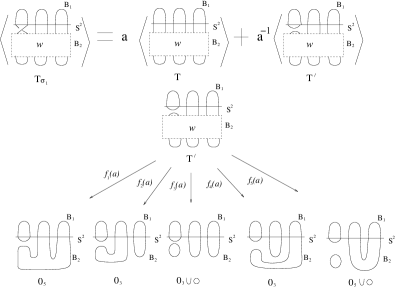
Figure 7.

Therefore, $<T_{\sigma_{1}}>=a<T>+a^{-1}<T^{\prime}>=a(f_{1}(a)\mathcal{A}+f_{2}(a)\mathcal{B}+f_{3}(a)\mathcal{C}+f_{4}(a)\mathcal{D}+f_{5}(a)\mathcal{E})+a^{-1}(f_{1}(a)\mathcal{E}+f_{2}(a)\mathcal{C}+kf_{3}(a)\mathcal{C}+f_{4}(a)\mathcal{C}+kf_{5}(a)\mathcal{E})=af_{1}(a)\mathcal{A}+af_{2}(a)\mathcal{B}+(af_{3}(a)+a^{-1}(f_{2}(a)+kf_{3}(a)+f_{4}(a)))\mathcal{C}+af_{4}(a)\mathcal{D}+(af_{5}(a)+a^{-1}(f_{1}(a)+kf_{5}(a)))\mathcal{E}.$

So, we have $f^{\prime}_{1}(a)=af_{1}(a)$, $f^{\prime}_{2}(a)=af_{2}(a)$, $f^{\prime}_{3}(a)=af_{3}(a)+a^{-1}(f_{2}(a)+kf_{3}(a)+f_{4}(a))$, $f^{\prime}_{4}(a)=af_{4}(a)$ and $f^{\prime}_{5}(a)=af_{5}(a)+a^{-1}(f_{1}(a)+kf_{5}(a))$.

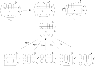
Figure 8.

Similarly, By Figure 8, we have $<T_{\sigma_{1}^{-1}}>=a<T^{\prime}>+a^{-1}<T>$.

Therefore, $<T_{\sigma_{1}^{-1}}>=a<T^{\prime}>+a^{-1}<T>=a(f_{1}(a)\mathcal{E}+f_{2}(a)\mathcal{C}+kf_{3}(a)\mathcal{C}+f_{4}(a)\mathcal{C}+kf_{5}(a)\mathcal{E})+a^{-1}(f_{1}(a)\mathcal{A}+f_{2}(a)\mathcal{B}+f_{3}(a)\mathcal{C}+f_{4}(a)\mathcal{D}+f_{5}(a)\mathcal{E})=a^{-1}f_{1}(a)\mathcal{A}+a^{-1}f_{2}(a)\mathcal{B}+(a^{-1}f_{3}(a)+a(f_{2}(a)+kf_{3}(a)+f_{4}(a)))\mathcal{C}+a^{-1}f_{4}(a)\mathcal{D}+(a^{-1}f_{5}(a)+a(f_{1}(a)+kf_{5}(a)))\mathcal{E}.$

So, we have $f^{\prime}_{1}(a)=a^{-1}f_{1}(a)$, $f^{\prime}_{2}(a)=a^{-1}f_{2}(a)$, $f^{\prime}_{3}(a)=a^{-1}f_{3}(a)+a(f_{2}(a)+kf_{3}(a)+f_{4}(a))$, $f^{\prime}_{4}(a)=a^{-1}f_{4}(a)$ and $f^{\prime}_{5}(a)=a^{-1}f_{5}(a)+a(f_{1}(a)+kf_{5}(a))$.

This operations can be expressed by the following.

$\left[\begin{array}[]{ccccc}a^{\pm 1}&0&0&0&0\\ 0&a^{\pm 1}&0&0&0\\ 0&a^{\mp 1}&a^{\pm 1}+a^{\mp 1}k&a^{\mp 1}&0\\ 0&0&0&a^{\pm 1}&0\\ a^{\mp 1}&0&0&0&a^{\pm 1}+a^{\mp 1}k\\ \end{array}\right]$ $\left[\begin{array}[]{c}f_{1}(a)\\ f_{2}(a)\\ f_{3}(a)\\ f_{4}(a)\\ f_{5}(a)\\ \end{array}\right]=\left[\begin{array}[]{c}f_{1}^{\prime}(a)\\ f_{2}^{\prime}(a)\\ f_{3}^{\prime}(a)\\ f_{4}^{\prime}(a)\\ f_{5}^{\prime}(a)\\ \end{array}\right]$

Similarly, we have four more operations from $\sigma_{2}^{\pm 1},\sigma_{3}^{\pm 1}$, $\sigma_{4}^{\pm 1}$ and $\sigma_{5}^{\pm 1}$ as follows.

$\left[\begin{array}[]{ccccc}a^{\pm 1}+a^{\mp 1}k&0&0&a^{\mp 1}&a^{\mp 1}\\ 0&a^{\pm 1}+a^{\mp 1}k&a^{\mp 1}&0&0\\ 0&0&a^{\pm 1}&0&0\\ 0&0&0&a^{\pm 1}&0\\ 0&0&0&0&a^{\pm 1}\\ \end{array}\right]\left[\begin{array}[]{c}f_{1}(a)\\ f_{2}(a)\\ f_{3}(a)\\ f_{4}(a)\\ f_{5}(a)\\ \end{array}\right]=\left[\begin{array}[]{c}f_{1}^{\prime}(a)\\ f_{2}^{\prime}(a)\\ f_{3}^{\prime}(a)\\ f_{4}^{\prime}(a)\\ f_{5}^{\prime}(a)\\ \end{array}\right]$

$\left[\begin{array}[]{ccccc}a^{\pm 1}&0&0&0&0\\ 0&a^{\pm 1}&0&0&0\\ 0&a^{\mp 1}&a^{\mp 1}k+a^{\pm 1}&0&a^{\mp 1}\\ a^{\mp 1}&0&0&a^{\mp 1}k+a^{\pm 1}&0\\ 0&0&0&0&a^{\pm 1}\\ \end{array}\right]\left[\begin{array}[]{c}f_{1}(a)\\ f_{2}(a)\\ f_{3}(a)\\ f_{4}(a)\\ f_{5}(a)\\ \end{array}\right]=\left[\begin{array}[]{c}f_{1}^{\prime}(a)\\ f_{2}^{\prime}(a)\\ f_{3}^{\prime}(a)\\ f_{4}^{\prime}(a)\\ f_{5}^{\prime}(a)\\ \end{array}\right]$

$\left[\begin{array}[]{ccccc}a^{\pm 1}+a^{\mp 1}k&a^{\mp 1}&0&a^{\mp 1}&0\\ 0&a^{\pm 1}&0&0&0\\ 0&0&a^{\pm 1}&0&0\\ 0&0&0&a^{\pm 1}&0\\ 0&0&a^{\mp 1}&0&a^{\pm 1}+a^{\mp 1}k\\ \end{array}\right]\left[\begin{array}[]{c}f_{1}(a)\\ f_{2}(a)\\ f_{3}(a)\\ f_{4}(a)\\ f_{5}(a)\\ \end{array}\right]=\left[\begin{array}[]{c}f_{1}^{\prime}(a)\\ f_{2}^{\prime}(a)\\ f_{3}^{\prime}(a)\\ f_{4}^{\prime}(a)\\ f_{5}^{\prime}(a)\\ \end{array}\right]$

$\left[\begin{array}[]{ccccc}a^{\pm 1}&0&0&0&0\\ a^{\mp 1}&a^{\pm 1}+a^{\mp 1}k&0&0&0\\ 0&0&a^{\pm 1}+a^{\mp 1}k&a^{\mp 1}&a^{\mp 1}\\ 0&0&0&a^{\pm 1}&0\\ 0&0&0&0&a^{\pm 1}\\ \end{array}\right]\left[\begin{array}[]{c}f_{1}(a)\\ f_{2}(a)\\ f_{3}(a)\\ f_{4}(a)\\ f_{5}(a)\\ \end{array}\right]=\left[\begin{array}[]{c}f_{1}^{\prime}(a)\\ f_{2}^{\prime}(a)\\ f_{3}^{\prime}(a)\\ f_{4}^{\prime}(a)\\ f_{5}^{\prime}(a)\\ \end{array}\right]$, where    $k=-a^{2}-a^{-2}.$

Recall that $T$ is expressed by $\sigma_{k_{1}}^{\epsilon_{1}}\sigma_{k_{2}}^{\epsilon_{2}}\cdot\cdot\cdot\sigma_{k_{n-1}}^{\epsilon_{n-1}}\sigma_{k_{n}}^{\epsilon_{n}}$ for some non-zero integers $\epsilon_{i}$ ($1\leq i\leq n$), where $k_{i}\in\{1,2,3,4,5\}$.

Then, we know that the generators $\sigma_{i}$ corresond to $B_{i}$.

So, given $B=B_{k_{1}}^{\epsilon_{1}}B_{k_{2}}^{\epsilon_{2}}\cdot\cdot\cdot B_{k_{n-1}}^{\epsilon_{n-1}}B_{k_{n}}^{\epsilon_{n}}$ , we have

$<T>=f_{1}(a)<T_{1}>\mathcal{A}+f_{2}(a)\mathcal{B}+f_{3}(a)\mathcal{C}+f_{4}(a)\mathcal{D}+f_{5}(a)\mathcal{E}$

for $[f_{1}(a)~{}f_{2}(a)~{}f_{3}(a)~{}f_{4}(a)~{}f_{5}(a)]^{t}=B[0~{}0~{}1~{}0~{}0]^{t}$ since $<T_{0_{3}}>=0\cdot\mathcal{A}+0\cdot\mathcal{B}+1\cdot\mathcal{C}+0\cdot\mathcal{D}+0\cdot\mathcal{E}$.

From $<T>$, we have $<K>=f_{1}(a)+k(f_{2}(a)+f_{4}(a)+f_{5}(a))+k^{2}f_{3}(a)$ since $\overline{T_{0_{1}}}$ is the unknot, $\overline{T_{0_{i}}}$ for $i\in\{2,4,5\}$ are disjoint union of two unknots and $\overline{T_{0_{3}}}$ is disjoint union of three unknots as in Figure 8.

Therefore, $X_{K}=(-a^{-3})^{w(\overrightarrow{K})}(f_{1}(a)+k(f_{2}(a)+f_{4}(a)+f_{5}(a))+k^{2}f_{3}(a))$ ∎

We remark that the matrices $B_{1}^{\pm 1},B_{2}^{\pm 1},B_{3}^{\pm 1}$, $B_{4}^{\pm 1}$ and $B_{5}^{\pm 1}$ satisify the braid group relations.

4. The Kauffman brackets of $2n$-plat presentation knots

We define the bracket polynomial of the rational $n$-tangle $T$ as $<T>=f^{T}_{1}(a)<{0_{1}}>+f^{T}_{2}(a)<{0_{2}}>+\cdot\cdot\cdot+f^{T}_{m}<{0_{m}}>$, where $f^{T}_{i}(a)$ are Laurent polynomials that are obtained by starting with $T$ and using the three axioms repeatedly until only the $m$ trivial tangles $<{0_{j}}>$ in the expression given for $T$ are left.

So, we remark that the number $m$ of trivial rational $n$-tangles ${0_{i}}$ needs to be calculated.

To do this, let $\psi(0)=1$. Then we define the map $\psi:2\mathbb{Z}^{+}\rightarrow\mathbb{Z}^{+}$ so that $\psi(2k)=\sum_{i=1}^{k}\psi(2i-2)\cdot\psi(2k-2i)$.

Lemma 4.1.

The number of trivial rational $n$-tangles is $\psi(2n)$.

Proof.

Let ${0_{i}}$ be a trivial rational $n$-tangle. Then we note that the string with the endpoint $1$ has the other endpoint at $2k+1$ for some positive integer $k$.

If $k=1$ then we calculate the number of trivial $n$-tangles by considering $2n-2$ endpoints and it is $\phi(0)\cdot\psi(2n-2)$.

If $k=2$ then we have a nested string inside of the string with the endpoint $1$ and we need to calculate the possible case for the rest of strings. Then it is $\psi(2)\cdot\psi(2n-4)$.

By considering the all subcases with respect to $k$, we calculate the number of trivial rational $n$-tangle which is $\sum_{i=1}^{n}\psi(2i-2)\cdot\psi(2n-2i)$.

Therefore, the number of trivial rational $n$-tangles is $\psi(2n)$.

∎

Recall $\overline{T}$ that is the tangle closure of the tangle $T$ to have the knot with the $2n$-plat presentation.

Now, we have a corollary to calculate the Kauffman polynomial of $n$-plat presentation as follows.

Corollary 4.2.

There exist $(4n-2)$ $\psi(2n)\times\psi(2n)$ matrices to calculate the coefficents $f^{T}_{1}(a),...,f^{T}_{\psi(2n)}(a)$ of the Kauffman bracket for a rational $n$-tangle $T$ with a $2n$-plat presentation ${q_{2n}(w)}$. Moreover, we calculate the Kauffman bracket of $\overline{q_{2n}(w)}$ and the Kauffman polynomial of $\overline{q_{2n}(w)}$ from this.

Proof.

This is the generalization of Theorem 2.1. ∎

5. A way to calculate the writhe of a $n$-bridge knot ($n\geq 2$)

First, assume that the projection onto the $xy$-plane of a $n$-bridge knot $K$ has a plat presentaion $p_{2n}(w)$ with $w=\sigma_{k_{1}}^{\epsilon_{1}}\sigma_{k_{2}}^{\epsilon_{2}}\cdot\cdot\cdot\sigma_{k_{m-1}}^{\epsilon_{m-1}}\sigma_{k_{m}}^{\epsilon_{m}}$ for some non-zero integers $\epsilon_{i}$ ($1\leq i\leq m$), where $k_{i}\in\{1,2,\cdot\cdot\cdot,2n-1\}$ and $k_{j}\neq k_{j+1}$ for $1\leq j\leq m-1$.

Then we have the plat presentation $q_{2n}(w)$ of the tangle $T=K\cap B_{2}$ so that $\overline{q_{2n}(w)}=p_{2n}(w)$.

Let $\mathcal{P}(\sigma_{i}^{\pm 1})$ be the $2n\times 2n$ matrix which is obtained by interchanging the $i$th and $i+1$st rows of $I$. Then $\mathcal{P}$ extends to a homomorphism from $\mathbb{B}_{2n}$ to $GL_{6}(\mathbb{Z})$.

For an element $w$ of $\mathbb{B}_{2n}$, let 1,2,…,$2n$ be the upper endpoints of the $2n$ strings numbered from the left. Then let $\delta_{i}$ be the trivial arc components of $p_{2n}(w)\cap p(B_{1})$ so that $\partial\delta_{i}=\{2i-1,2i\}$. Also, let $\gamma_{j}$ be the trivial arcs which connect pairs of consecutive strings of the braid at the bottom endpoints numbered from the left. Let $u=[1,2,\cdot\cdot\cdot,2n]$. Then we assign the same number to the bottom endpoint of the $2n$ strings. Then we say that the new ordered sequence of numbers $w(u)$ is the permutation induced by $w$.

Lemma 5.1.

$w(u)=[1,2,\cdot\cdot\cdot,2n]\mathcal{P}(w)$.

Proof.

This is proven by induction on $l=|\epsilon_{1}|+|\epsilon_{2}|+\cdot\cdot\cdot+|\epsilon_{m}|$.

∎

Let $R$ be the $2n\times 2n$ matrix which is obtained by interchanging the $2i+1$st and $2i+2$nd rows of $I$ for all $i$ such that $0\leq i\leq n-1$.

Recall that $w^{r}$ is the reverse word of $w$.

Let $[o_{j}(1),o_{j}(2),\cdot\cdot\cdot,o_{j}(2n)]=[1,2,\cdot\cdot\cdot,2n](\mathcal{P}(w)R\mathcal{P}(w^{r})R)^{j-1}\mathcal{P}(w)R\mathcal{P}(w^{r})$ for $1\leq j\leq n$.

Also, let $[o_{j}^{\prime}(1),o_{j}^{\prime}(2),\cdot\cdot\cdot,o_{j}^{\prime}(2n)]=[1,2,\cdot\cdot\cdot,2n](\mathcal{P}(w)R\mathcal{P}(w^{r})R)^{j}$ for $0\leq j\leq n$.

We note that $[o_{0}^{\prime}(1),o_{0}^{\prime}(2),\cdot\cdot\cdot,o_{0}^{\prime}(2n)]=u$.

Consider the case that $j=1$. In order to get $[1,2,\cdot\cdot\cdot,2n]\mathcal{P}(w)$, we follow the strings of the braid down while preserving the numbers of the strings. Then $[1,2,\cdot\cdot\cdot,2n]\mathcal{P}(w)R$ is obtained by following along the trivial arcs $\gamma_{i}$ while preserving the numbers of the strings. Then we follow the strings of the braid up while preserving the numbers of the strings to get $[1,2,\cdot\cdot\cdot,2n]\mathcal{P}(w)R\mathcal{P}(w^{r})$ which is $[o_{1}(1),o_{1}(2),\cdot\cdot\cdot,o_{1}(2n)]$. After this, we follow along the trivial arcs $\delta_{i}$ while preserving the numbers of the strings to get $[1,2,\cdot\cdot\cdot,2n]\mathcal{P}(w)R\mathcal{P}(w^{r})R$ which is $[o_{1}^{\prime}(1),o_{1}^{\prime}(2),\cdot\cdot\cdot,o_{1}^{\prime}(2n)]$.

Generally speaking, from the $[o_{j}^{\prime}(1),o_{j}^{\prime}(2),\cdot\cdot\cdot,o_{j}^{\prime}(2n)]$ we follow the strings of the braid down and follow along the trivial arcs $\gamma_{i}$ and follow the strings of the braid up to get $[o_{j+1}(1),o_{j+1}(2),\cdot\cdot\cdot,o_{j+1}(2n)]$ while preserving the numbers of the strings. Then, we get $[o^{\prime}_{j+1}(1),o^{\prime}_{j+1}(2),\cdot\cdot\cdot,o^{\prime}_{j+1}(2n)]$ by following along the trivial arcs $\delta_{i}$ while preserving the numbers of the strings.

We note that $o^{\prime}_{0}(i)=i,o^{\prime}_{1}(i),\cdot\cdot\cdot o^{\prime}_{n-1}(i)$ are distinct points. Otherwise, $K$ is a link, not a knot. Also, we know that $o^{\prime}_{j}(i)=o^{\prime}_{n+j}(i)$.

Similarly, $o_{1}(i),o_{2}(i),\cdot\cdot\cdot o_{n}(i)$ are distinct points and $o_{j}(i)=o_{n+j}(i)$.

Also, we note that for a trivial arc $\delta_{k}$ there exists a unique $i$ ($1\leq i\leq n$) so that either $o_{i}(1)=2k-1$ or $o_{i}(1)=2k$.

Without loss of generality, give the clockwise orientation to the trivial arc $\delta_{1}$ in $B_{1}$ with $\partial\delta_{1}=\{1,2\}$ from $1$ to $2$ along $\delta_{1}$. So, the initial point of $\delta_{1}$ is 1 and the terminal point of $\delta_{1}$ is 2 for the given orientation. Then, the orientations of the other trivial arcs $\delta_{2},\cdot\cdot\cdot,\delta_{n}$ in $B_{1}$ are determined by the orientation of the knot $K$ which is induced by $\delta_{1}$.

Lemma 5.2.

The trivial arc $\delta_{k}$ has the same clockwise orientation as $\delta_{1}$ if $k=o_{i}(1)/2$ for some $i$ ($1\leq i\leq n$). The trivial arc $\delta_{k}$ has the opposite orientation (counterclockwise) as $\delta_{1}$ if $k=(o_{i}(1)+1)/2$ for some $i$ ($1\leq i\leq n$).

Proof.

If $k=o_{i}(1)/2$ for some $i$ then the endpoints of $\delta_{k}$ are $o_{i}(1)-1$ and $o_{i}(1)$. Also, the orientation of $\delta_{k}$ is from $o_{i}(1)-1$ to $o_{i}(1)$. Therefore, the $\delta_{k}$ has the same orientaion as $\delta_{1}$.

If $k=(o_{i}(1)+1)/2$ for some $i$ then the endpoints of $\delta_{k}$ are $o_{i}(1)$ and $o_{i}(1)+1$. Also, the orientation of $\delta_{k}$ is from $o_{i}(1)+1$ to $o_{i}(1)$. Therefore, the $\delta_{k}$ has the opposite orientation as $\delta_{1}$. ∎

Recall the ordered sequence of numbers $u=[1,2,\cdot\cdot\cdot,2n]$. Now, we define a new sequence of numbers $r=[r(1),r(2),\cdot\cdot\cdot,r(2n)]$ as follows. For the orientation given above, we replace the original numbers of $u=[1,2,...,2n]$ for the initial points of $\delta_{i}$ by 1 and we replace the original numbers for the terminal points of $\delta_{i}$ by 2.

Now, let $r_{0}=r$.

Let $r_{i}=[r_{i}(1),r_{i}(2),r_{i}(3),\cdot\cdot\cdot,r_{i}(2n)]=r\mathcal{P}(\sigma_{k_{1}}^{\epsilon_{1}}\sigma_{k_{2}}^{\epsilon_{2}}\cdot\cdot\cdot\sigma_{k_{i-1}}^{\epsilon_{i-1}}\sigma_{k_{i}}^{\epsilon_{i}})$ for $1\leq i\leq m$.

Let $v(i)=\left\{\begin{array}[]{cl}0&$if~{}$r_{i-1}(k_{i})=r_{i-1}(k_{i}+1)\\ 1&$if~{}$r_{i-1}(k_{i})\neq r_{i-1}(k_{i}+1)\\ \end{array}\right.$

Then we calculate the writhe of $K$ as follows.

Theorem 5.3.

$w(K)=\sum_{i=1}^{m}(-1)^{v(i)}\epsilon_{i}$.

Proof.

For the $2n$ strings of the braid $w$, we assign the number $r(k)$ to each string with the upper endpoint $k$ for $1\leq k\leq 2n$.

Without loss of generality, we give the orientation (clockwise) to $\delta_{1}$ from $1$ to $2$ along $\delta_{1}$. Then the orientation at 1 is up and the orientation at 2 is down. Then we know that the orientation at $j$ is up if $r(j)=1$ and it is down if $r(j)=2$.

Fix a value $i$ ($1\leq i\leq m$).

Case 1: Suppose that $r_{i-1}(k_{i})=r_{i-1}(k_{i}+1)$.

Then the two strings for the ($\sum_{j=1}^{i-1}|\epsilon_{j}|+1)$-th crossing have the same orientation since $r_{i-1}(k_{i})=r_{i-1}(k_{i}+1)$, i.e., the numbers of the two strings for ($\sum_{j=1}^{i-1}|\epsilon_{j}|+1)$-th crossing are the same. If $r_{i-1}(k_{i})=r_{i-1}(k_{i}+1)=1$ then the orientations are up and if $r_{i-1}(k_{i})=r_{i-1}(k_{i}+1)=2$ then the orientations are down.

Then we note that the index $e$ of ($\sum_{j=1}^{i-1}|\epsilon_{j}|+1)$-th crossing is $+1$ if the crossing is positive and the index $e$ of ($\sum_{j=1}^{i-1}|\epsilon_{j}|+1)$-th crossing is $-1$ if the crossing is negative.

We note that all the crossings in $\sigma_{k_{i}}^{\epsilon_{i}}$ have the same index.

Therefore, the contribution of $\sigma_{k_{i}}^{\epsilon_{i}}$ to the writhe is $\epsilon_{i}$

Since $v(i)=0$, we check that $(-1)^{v(i)}\epsilon_{i}=(-1)^{0}\epsilon_{i}=\epsilon_{i}$ is the contribution of $\sigma_{k_{i}}^{\epsilon_{i}}$ to the writhe.

Case 2: Suppose that $r_{i-1}(k_{i})\neq r_{i-1}(k_{i}+1)$ .

Then we know that the orientations of the two strings for ($\sum_{j=1}^{i-1}|\epsilon_{j}|+1)$-th crossing are either up and down or down and up since $r_{i-1}(k_{i})\neq r_{i-1}(k_{i}+1)$.

So, we check that the index $e$ of ($\sum_{j=1}^{i-1}|\epsilon_{j}|+1)$-th crossing is $-1$ if the crossing is positive and the index $e$ of ($\sum_{j=1}^{i-1}|\epsilon_{j}|+1)$-th crossing is $+1$ if the crossing is negative.

Therefore, the contribution of $\sigma_{k_{i}}^{\epsilon_{i}}$ to the writhe is $-\epsilon_{i}$

Since $v(i)=1$, we check that $(-1)^{v(i)}\epsilon_{i}=(-1)\epsilon_{i}=-\epsilon_{i}$ is the contribution of $\sigma_{k_{i}}^{\epsilon_{i}}$ to the writhe.

By adding all the indices of $\sigma_{k_{i}}^{\epsilon_{i}}$, we have the given formula for the writhe. ∎

Department of Mathematics, Oklahoma State University, 401 Mathematical Sciences, Stillwater, OK 74078, USA

References

[1] C.C. Adams: The knot book, W.H. Freeman and Co. (1994), Chapters 1-6.
[2] J. Birman: Braids, links and mapping class groups, Annals of Math. Studies 82,
Princeton Univ. Press, 1974.
[3] J. Birman, T. Kanenobu: Jones’ braid-plat formula and a new surgery triple,
Proc. Amer. Math. Soc (1988), Vol 102, no. 3.
[4] H. Cabrera-Ibarra: On the classification of rational 3-tangles, J. Knot Theory Ramifications 12 (2003), no. 7, 921-946.
[5] S. Eliahou, L.H. Kauffman, M.B. Thistlethwaite: Infinite families of links with trivial Jones polynomial, Topololy (2003), no. 42, 155-169.
[6] J. Emert, C. Ernst: N-string tangles, J. Knot Theory Ramifications 9 (2000), no. 9, 987–1004.
[7] J.R. Goldman, L.H. Kauffman: Rational tangles. Adv. in Appl. Math (1997), no. 3, 300-332.
[8] V. F. R. Jones: A polynomial invariant for knots via von Neumann algebras, Bull. Amer. Math. Soc. 12 (1985), 103-111.
[9] L.H. Kauffman: State models and the Jones polynomial. Topology 26 (1987), no. 3, 395-407.
[10] L.H. Kauffman, S. Lambropoulou: On the classification of rational tangles.
Adv. in Appl. Math. 33 (2004), no. 2, 199–237