Weber’s optimal stopping problem and generalizations

Abstract.

One way to interpret the classical secretary problem (CSP) is to consider it as a special case of the following problem. We observe $n$ independent indicator variables $I_{1},I_{2},\dotsc,I_{n}$ sequentially and we try to stop on the last variable being equal to 1. If $I_{k}=1$ it means that the $k$-th observed secretary has smaller rank than all previous ones (and therefore is a better secretary). In the CSP $p_{k}=E(I_{k})=1/k$ and the last $k$ with $I_{k}=1$ stands for the best candidate. The more general problem of stopping on a last “1” was studied by Bruss (2000). In what we will call Weber’s problem the variables $I_{k}$ can take more than two values and we try to stop on the last occurence of one of these values. Notice that we do not know in advance the value taken by the variable on which we stop.

We can solve this problem in some cases and provide algorithms to compute the optimal stopping rule. These cases carry enough generality to be applicable in concrete situations.

1. Statement of the type of Problems

The following problem has been proposed in 2013 by Weber (R. R. Weber, University of Cambridge) to his students.

1.1. Problem 1 (Weber’s problem)

A financial advisor tries to impress his clients if immediately following a week in which the ftse index moves by more than 5% in some direction he correctly predicts that this is the last week during the calendar year that it moves more than 5% in that direction.

Suppose that in each week the change in the index is independently up by at least 5%, down by at least 5% or neither of these, with probabilities $p$, $p$ and $1-2p$ respectively ($p\leq 1/2$). He makes at most one prediction this year. With what strategy does he maximize the probability of impressing his clients?

The solution by backwards induction is relatively straightforward and several students of Weber’s found the solution for this specific problem. Weber then discussed with Bruss (private communication 2013) several modifications of this problem. The objective of the present paper is to present the solutions of two Bruss-Weber modifications which have an appeal for applications.

We present two modifications of Problem 1. We code a “1” if the index goes up by some fixed percentage some day, “$-1$” if it goes down by some (other) fixed percentage and “0” else. Two other ways of generalization come to our mind. One can imagine that the probabilities of a “$1$” and of a “$-1$” are different, we then have two parameters $p$ and $p^{\prime}$. One can also imagine that the probabilities of a “1” or “$-1$” are equal but are allowed to differ day after day. We then have $n$ parameters $(p_{k},k=1,\dots,n)$, thus also generalizing Bruss’ problem of stopping on a alast specific success. This also opens the way to tackle continuous time problems with a random number of decision items (see Bruss (2000)). In this paper we confine our interest to the discrete time setting, however.

The integer $n$ is always known and represents the number of observations of the index made over the time horizon. In Weber’s problem, the model is as follows. We call $n$ the length of the horizon. Let $X_{1},X_{2},\dotsc,X_{n}$ ($n$ known) be i.i.d. random variables, such that

$$P(X_{i}=1)=P(X_{i}=-1)=p\quad\text{and}\quad P(X_{i}=0)=1-2p.$$

Let $(\mathcal{F}_{k})_{k=1,2,\dotsc}$ be the filtration generated by $X_{1},X_{2},\dotsc,X_{k}$. We want to find, among all random times $\tau$, the stopping time $\tau^{\star}$ maximizing the quantity

(1) $$E\left(\mathbbm{1}\biggl{[}\biggl{(}\left\{X_{\tau}=1\right\}\cap\bigcap_{i=\tau+1}^{n}\left\{X_{i}\neq 1\right\}\biggr{)}\cup\biggl{(}\left\{X_{\tau}=-1\right\}\cap\bigcap_{i=\tau+1}^{n}\left\{X_{i}\neq-1\right\}\biggr{)}\biggr{]}\right).$$

Remark. Note that stopping on a “$1$” or a “$-1$” may be a stopping time but stopping on a last “1” or “-1” is in general not a stopping time. Adding the conditional knowledge $\mathcal{F}_{k}$ in the expectation we obtain a stopping time. However this can be dropped because of the markovian nature of the problem. Indeed, all that counts at a given time $k$ is the value of $I_{k}$ and the number of remaining variables. The knowledge of the history therefore does not influence our decision at any given time.

We now describe quickly the two modifications of Problem 1.

1.2. Problem 2

The difference between this problem and Problem 1 is that here the probability of a “$1$” is different from that of a “$-1$”. This problem is therefore described by three parameters: $n$, $p$ and $p^{\prime}$ which are the number of variables, the probability of a variable equal to $1$ and the probability a variable equal to $-1$, respectively.

1.3. Problem 3

Another interesting modification is to look at the problem of a “same $p$” for $+1$’s and $-1$’s but one that is changing over time. Formally, the problem is described by the parameters $n$ and $p_{1},p_{2},\dotsc,p_{n}$ where $p_{k}=P(X_{k}=1)=P(X_{k}=-1)$.

We state them and we provide optimal decision rules. Our special interest is to make these solutions as quick and concise as possible.

2. Solution of Problem 2

We are looking at the case where the probabilities of a “1” or a “$-1$” are not necessarily equal. The variables $X_{1},X_{2},\dotsc,X_{n}$ are i.i.d with $p:=P(X_{1}=1)$, $p^{\prime}:=P(X_{1}=-1)$ and $P(X_{1}=0)=1-p-p^{\prime}$, $p,p^{\prime}\in[0,1]$. Without loss of generality we will suppose that $p\geq p^{\prime}$. We must suppose that $p+p^{\prime}\leq 1$. If $p+p^{\prime}=1$ the problem is trivial since it suffices to stop on the last event. If $p^{\prime}=0$, Bruss’ odds-theorem and the accompanying algorithm gives the optimal strategy. Therefore we will suppose that $p,p^{\prime}\in(0,1)$ and, to avoid trivial cases, that $p+p^{\prime}<1$. The notations $q=1-p$, $q^{\prime}=1-p^{\prime}$ and ${\tilde{q}}=1-p-p^{\prime}$ will be used thoughout the article.

2.1. Monotonicity and unimodality

In this section we state and prove several lemmas that will be the basis of the solving algorithm.

We will show that the problem is monotone, that is, if at a certain time index it is optimal to stop on a “1” (respectively on a “$-1$”), then it is optimal to stop on a “1” (respectively on a “$-1$”) at any later time index. Assaf and Samuel-Cahn (2000) called such stopping rules “simple”.

Lemma 1.

The problem described in Problem 2 is monotone.

Proof.

Let $v_{j}$ be the optimal probability of a win when there are still $j$ variables to observe. It is optimal to stop at stage $k\in\left\{1,2,\dots,n\right\}$ if $X_{k}=1$ and

(2) $$q^{n-k}>v_{n-k},$$

by definition of $v_{n-k}$. We now show that (2) implies $q^{n-k-1}>v_{n-k-1}$. From independence and the optimality principle we have

$$v_{n-k}=p(v_{n-k-1}\vee q^{n-k-1})+p^{\prime}(v_{n-k-1}\vee(q^{\prime})^{n-k-1})+(1-p-p^{\prime})v_{n-k-1},$$

where $a\vee b$ denotes the maximum of $a$ and $b$. Also, $\max\{v_{n-k-1},q^{n-k-1},(q^{\prime})^{n-k-1}\}\geq v_{n-k-1}$, and thus by inequality (2) we obtain

$$q^{n-k-1} >\bigl{(}pv_{n-k-1}+p^{\prime}v_{n-k-1}+(1-p-p^{\prime})v_{n-k-1}\bigr{)}q^{-1}$$

$$>v_{n-k-1},\qquad 0\leq k\leq n-1.$$

This shows monotonicity with respect to the stopping problem of the “1”’s. An analoguous argument proves monotonicity for the value $-1$. Hence the lemma is proved. ∎

Since $p\geq p^{\prime}$, we expect a different behaviour regarding the 1’s and the $-1$’s, and this will become apparent in what follows. For $j,k\in\left\{1,2,\dotsc,n\right\}$, we use the following notations

$$\tau^{+}_{j} =\inf\left\{j\leq m\leq n:X_{m}=1\right\}\wedge n,$$

$$\tau^{-}_{k} =\inf\left\{k\leq m\leq n:X_{m}=-1\right\}\wedge n,$$

$$\tau_{j,k} =\tau^{+}_{j}\wedge\tau^{-}_{k},$$

with $x\wedge y=\min\left\{x,y\right\}$ and the usual convention that $\inf\varnothing=+\infty$. The monotonicity of the problem implies that there are two indexes $s$ and $s^{\prime}$ such that the stopping time $\tau_{s,s^{\prime}}$ is optimal, that is, maximizes (1).

Consider a stopping region (or stopping set) as follows

(3) $$R=\left\{(k,1):k\in J^{+}\right\}\cup\left\{(k,-1):k\in J^{-}\right\}\cup\left\{(n,0)\right\}$$

where $J^{+}$ and $J^{-}$ are subsets of $\left\{1,2,\dotsc,n\right\}$. A stopping time for this problem can be defined as the first $k\in\left\{1,2,\dotsc,n\right\}$ such that $(k,X_{k})\in R$, that is, the first hitting time of the set $R$ of the process $((k,X_{k}))_{1\leq k\leq n}$. This hitting time will be denoted $\tau_{R}$. For any stopping region $R$, we let $V_{R}$ be the probability of winning if our strategy is to we use the first hitting time of the set $R$.

Let $R^{\star}$ denote the optimal stopping region, that is,

(4) $$R^{\star}=\left\{(k,1):k\geq s\right\}\cup\left\{(k,-1):k\geq s^{\prime}\right\}\cup\left\{(n,0)\right\}.$$

By definition, the optimal value of the problem is $V:=V_{R^{\star}}$. We now have two lemmas:

Lemma 2.

If $R_{1}\subseteq R_{2}\subseteq R^{\star}$, then $V_{R_{1}}\leq V_{R_{2}}$.

Proof.

If $R_{1}=R_{2}$, there is nothing to prove. Let $R_{1}\neq R_{2}$ and $\underline{X}=(X_{1},X_{2},\dotsc,X_{n})$ and suppose that $\tau_{R_{2}}(\underline{X})\neq\tau_{R_{1}}(\underline{X})$. We necessarily have $\tau_{R_{2}}(\underline{X})<\tau_{R_{1}}(\underline{X})$ because $R_{1}\subseteq R_{2}$, and it is impossible to hit $R_{1}$ before $R_{2}$. We also have $s\leq\tau_{R^{\star}}(\underline{X})\leq\tau_{R_{2}}(\underline{X})$. Let $t=\tau_{R_{2}}(\underline{X})$. We assume that $X_{t}=1$. Let $\underline{X}^{\prime}=(0,0,\dotsc,0,1,X_{t+1},\dotsc,X_{n})$. Since $t$ is the first index $k$ after $s$ such that $X^{\prime}_{k}=1$ it is optimal to stop $\underline{X}^{\prime}$ at time $t$. We use the same argument if we stop on a $-1$. Therefore, the strategy based on $R_{2}$ does better than the strategy based on $R_{1}$.

On the set $\left\{\tau_{R_{1}}=\tau_{R_{2}}\right\}$, the two strategies perform the same. Overall, the strategy based on $R_{2}$ is better. ∎

Lemma 3.

If $R^{\star}\subseteq R_{1}\subseteq R_{2}$, then $V_{R_{1}}\geq V_{R_{2}}$.

Proof.

The arguments for this proof are analogous to those of the proof of the previous lemma and can be omitted. ∎

Finally, the following lemma allows, as we will see, for an efficient algorithm.

Lemma 4.

If $p\geq p^{\prime}$, then $s\geq s^{\prime}$.

Proof.

We must show that stopping on $X_{s}=-1$ is the optimal choice. In fact, we have, with the same notation as above,

$${(q^{\prime})}^{n-s}\geq q^{n-s}>v_{n-s},$$

and hence in particular $s\geq s^{\prime}$, since $q^{\prime}>q$. ∎

2.2. Recurrence equations for $w_{j,k}$

In this section we write the recurrence equations of the success probabilities of the stopping times $\tau_{j,k}$ defined in Section 2.1. Let $w_{j,k}=w^{(n)}_{j,k}$ denote the probability of a win if we use the stopping time $\tau_{j,k}$. If $j>k$, by conditionning on the value of $X_{k}$,

(5) $$\begin{aligned} w_{j,k}&=\sum_{\nu=-1,1,0}P(X_{j}=\nu)P(\text{win using $\tau^{+}_{j}\wedge\tau^{-}_{j}$}|X_{j}=\nu)\\ &=p^{\prime}{(q^{\prime})}^{n-k}+pw_{j,k+1}+(1-p-p^{\prime})w_{j,k+1}\\ &=p^{\prime}{(q^{\prime})}^{n-k}+q^{\prime}w_{j,k+1}.\end{aligned}$$

If $j=k$, we have

(6) $$w_{j,j}=p^{\prime}{(q^{\prime})}^{n-j}+pq^{n-j}+{\tilde{q}}w_{j+1,j+1}.$$

where ${\tilde{q}}=1-p-p^{\prime}$. We know that $w_{n,n}=p+p^{\prime}$ because the probability of a win using the strategy “stop on the last variable” is simply the probability that $X_{n}$ is not equal to zero.

Writing out these recurrence equations leads us to the following formulas:

(7) $$w_{j,j}=\frac{p}{p^{\prime}}(q^{n-j+1}-{\tilde{q}}^{n-j+1})+\frac{p^{\prime}}{p}({(q^{\prime})}^{n-j+1}-{\tilde{q}}^{n-j+1}),$$

and for $j>k$, we have

(8) $$w_{j,k}=(j-k)p^{\prime}{(q^{\prime})}^{n-k}+{(q^{\prime})}^{j-k}\biggl{(}\frac{p}{p^{\prime}}(q^{n-j+1}-{\tilde{q}}^{n-j+1})+\frac{p^{\prime}}{p}({(q^{\prime})}^{n-j+1}-{\tilde{q}}^{n-j+1})\biggr{)}.$$

If $j<k$ we use the same expression and exchange the role of $j$ and $k$.

2.3. Graphical illustrations

In the example displayed in figure 1, we choose $n=40$, $p=0.09$ and $p^{\prime}=0.05$. We find that the optimal thresholds are $(s,s^{\prime})=(33,28)$ and the optimal value is $v=w^{(40)}_{33,28}=0.52987\dots$. We plotted the $w_{j,k}$’s for this choice of $n$, $p$ and $p^{\prime}$. We notice that the maximum is obtained for $k_{+}=s$, $k_{-}=s^{\prime}$.

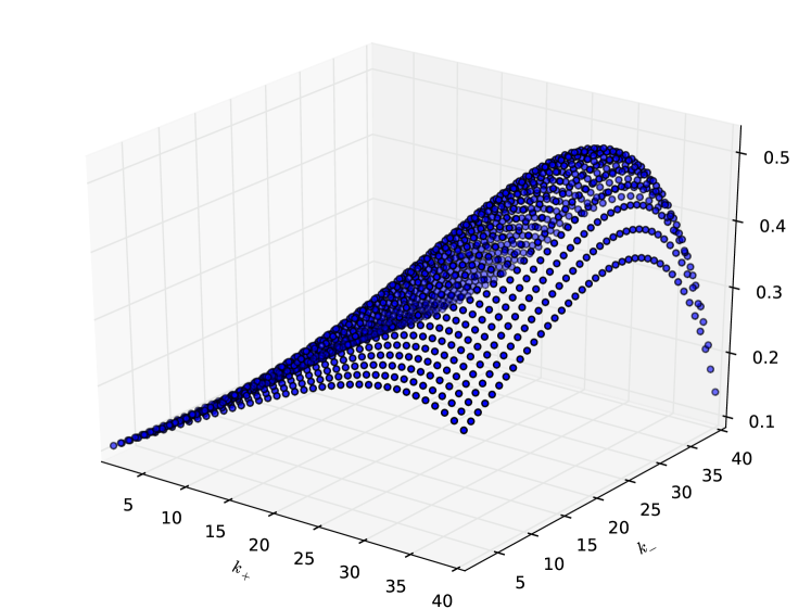
Figure 1. The plot shows the value $w_{k_{+},k_{-}}$, for a Problem 2-framework with $n=40$, $p=0.09$, $p^{\prime}=0.05$.

2.4. Solving algorithm

We present a first algorithm (see figure 2) based on the properties shown in Section 2.1. The idea of the algorithm is the following: if we start with the stopping region $R_{0}=\left\{(n,1),(n,0),(n,-1)\right\}$ and if we carefully add points to $R_{0}$, we will be able to detect the indexes $s$ and $s^{\prime}$, using the unimodality property.

The recurrence equations (5) and (6) can be used to speed up the computations of the $w_{j,k}$’s on lines 6, 12 and 23 in the algorithm.

1:Input : ($n,p,p^{\prime}$) 2:$k\leftarrow n$. 3:$\alpha\leftarrow w_{k,k}$ 4:Label1 5:if $k=1$ then $s:=1$, $s^{\prime}:=1$. 6:end if 7:$\beta\leftarrow w_{k,k-1}$ 8:if $\beta<\alpha$ then 9:     $s:=k$, $s^{\prime}:=k$, and stop. 10:else 11:     $\alpha\leftarrow\beta$ 12:     $k\leftarrow k-1$ 13:     $\beta\leftarrow w_{k,k}$ 14:     if $\beta<\alpha$ then 15:         $s:=k$ and go to Label2 16:     else 17:         $\alpha\leftarrow\beta$ 18:         go to Label1 19:     end if 20:end if 21:Label2 22:if $k=1$ then $s^{\prime}:=1$. 23:end if 24:$\beta\leftarrow w_{s,k-1}$ 25:if $\beta<\alpha$ then 26:     $s^{\prime}:=k$ and stop 27:else 28:     $\alpha\leftarrow\beta$ 29:     $k\leftarrow k-1$ 30:     go to Label2 31:end if

Figure 2. Pseudo-code for the algorithm giving the two optimal thresholds $s$ and $s^{\prime}$, in model 1. The input of the algorithm is $(n,p,p^{\prime})$.

2.5. Optimality of the computed thresholds

The lemmas of the above section do not guarantee that the indexes found in the algorithm are the true $s$ (line 13) and $s^{\prime}$. We must verify that if $s^{\prime}<s$, then $w_{s-1,s-1}\leq w_{s,s-1}$. This is true, because the two strategies $\tau_{s-1,s-1}$ and $\tau_{s,s-1}$ behave the same except in the case where $X_{s-1}=1$. Therefore, to compare $w_{s,s-1}$ against $w_{s-1,s-1}$, one can look at the same optimal stopping problem but with a number of variables being equal to $n-s$. In this case we see that the optimal strategy has success probability $w_{2,1}\geq w_{1,1}$ which is equal to the value $w_{s,s-1}\geq w_{s-1,s-1}$ of the initial problem with $n$ variables.

2.6. Formula-based algorithm

Here we use the explicit formula of the $w_{j,k}$’s given by (8). Note that this equation remains correct even if $j=k$. We also know that $s\geq s^{\prime}$ because $p>p^{\prime}$. As a result we know that we will not need to look at the value of $w_{j,k}$ for $j<k$. Therefore this is the only formula we need.

Another way of finding $s$ is by putting the second “$(-1)$-threshold” to 1, and comparing $w_{n,1}$ with $w_{n-1,1}$, then $w_{n-1,1}$ with $w_{n-2,1}$, etc. By an argument to the one used in Section 2.5, we can show that this determines correctly $s$.

We will use this and the unimodality of the function $j\mapsto w_{j,1}$ to find the index $s$. With a bisection algorithm this can be done in $O(\ln(n))$ time. When this first index is found, we look for the $k$ maximizing $k\mapsto w_{s,k}$.

An important feature of this method is that, for any $k\leq s^{\prime}$, the mode of the function $j\mapsto w_{j,k}$ occurs at index $s$.

In figure 3, we show information about the shape of the graph of the function $(j,k)\mapsto w_{j,k}$. Intuitively, if $k_{-}=n$, it is not likely that we win by selecting a “$-1$”. Therefore, we must concentrate on selecting a “$1$” only. The problem then becomes close to problem that the odds-algorithm can solve optimally.

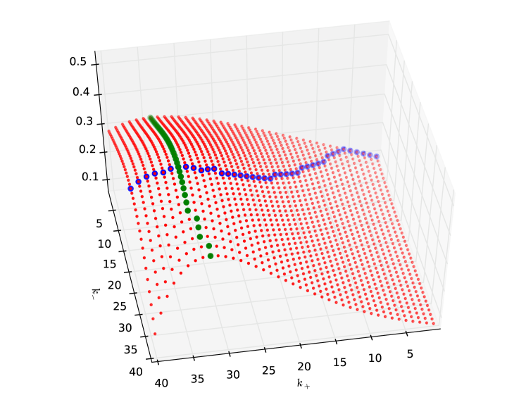
Figure 3. In this example (problem 2) we chose $(n,p,p^{\prime})=(40,0.1,0.05)$. The green dots show the modes, for $k_{-}=1,2,\dotsc,n$, of the functions $j\mapsto w_{j,k_{-}}$. The blue dots show the modes, for $k_{+}=1,2,\dotsc,n$, of the functions $k\mapsto w_{k_{+},k}$.

3. Solution of Problem 3

In this section we suppose that the variables $X_{1},X_{2},\dots,X_{n}$ are independent but have different distributions, that is, there are known parameters $p_{1},p_{2},\dotsc,p_{n}$ such that for all $1\leq i\leq n$,

$$P(X_{i}=1)=P(X_{i}=-1)=p_{i}\quad\text{and}\quad P(X_{i}=0)=1-2p_{i}.$$

We put as usual $q_{j}=1-p_{j}$.

3.1. Monotonicity

The proof of monotonicity of Section 2 can be adapted and using parameters $p_{k}$’s instead of one single parameter $p$ does not lengthen the proof.

By the same result about monotone stpping problems used in Section 1, we know that the 1-stage look-ahead rule is optimal (see Ferguson, 2008). Define

$$V_{k} =P\left(\text{we win by selecting the opportunity at stage $k$}|X_{k}\in\left\{-1,1\right\}\right)$$

and

$$W_{k} =w_{k+1,k+1}$$

where the $w_{j,k}$ have the same meaning as in the previous model. Obviously $V_{k}=\prod_{j=k+1}^{n}q_{j}$, and

$$W_{j} =\sum_{m=0}^{n-k-1}\left[\prod_{j=k+1}^{k+m}(1-2p_{j})\right](2p_{k+m+1})\left[\prod_{j=k+m+2}^{n}(1-p_{j})\right]$$

$$=2\sum_{m=0}^{n-k-1}\left[\prod_{j=k+1}^{k+m}(q_{j}-p_{j})\right]p_{k+m+1}\left[\prod_{j=k+m+2}^{n}q_{j}\right].$$

Therefore,

(9) $$\frac{W_{k}}{V_{k}}=2\sum_{m=0}^{n-k-1}\left[\prod_{j=k+1}^{k+m}(1-r_{j})r_{k+m+1}\right],$$

where $r_{j}=p_{j}/q_{j}$. It is not easy to extract the index $k^{\star}$ such that $W_{k}/V_{k}\geq 1$ for $k<k^{\star}$ and $W_{k}/V_{k}<1$ for $k\geq k^{\star}$. Nevertheless, we can provide an algorithm with linear complexity that will compute $k^{\star}$.

3.2. Computation of the stopping threshold

We must start by looking at the end of the sequence. If $W_{n-1}/V_{n-1}\geq 1$ we must stop on the last variable. If the ratio is smaller, then look at the ratio at time $n-2$, and so on. By starting with the end of the sequence we will only compute the values used in the expression of $W_{k^{\star}}/V_{k^{\star}}$.

Let $\Lambda_{k}=W_{k}/(2V_{k})$, $k=1,2,\dotsc,n-1$. We see that $\Lambda_{n-1}=r_{n}$. And we have the following recurrence equation

(10) $$\Lambda_{k}=r_{k+1}+(1-r_{k+1})\Lambda_{k+1},\qquad 1\leq k\leq n-2.$$

Here is, in pseudocode, the algorithm that computes the time index $k^{\star}$.

• Step 0 Set $k=n-1$. Compute $r_{n}$. We have $\Lambda_{n-1}=r_{n}$.

• Step 1 $k\leftarrow k-1$. Compute $r_{k+1}$, $1-r_{k+1}$ and $\Lambda_{k}=r_{k+1}+(1-r_{k+1})\Lambda_{k+1}$.

• Step 2 If $2\Lambda_{k}\geq 1$ then stop, and $k^{\star}=k+1$. If $2\Lambda_{k}<1$, go to step 1.

If $\Lambda_{1}<1$, set $k^{\star}=1$.

We see that the complexity of the algorithm is linear, and that the stopping time (1-sla) defined by

(11) $$n\wedge\inf\left\{k>k^{\star}:X_{k}\in\left\{-1,1\right\}\right\}$$

is optimal.

4. Particular case

If $p=p^{\prime}$ in model 1 or $p_{k}=p_{1}=:p$ for all $k$ in Problem 3, then we have the Weber’s original problem. In this case we use the method described in model 2 to obtain the optimal strategy. Since $V_{k}=q^{n-k}$ and $W_{k}=2((1-p)^{n-k}-(1-2p)^{n-k})$ we can describe the optimal stopping rule as: stop on the first variable equal to $1$ or equal to $-1$ after time $s$ ($s$ included), where $s$ is the smallest integer of $\left\{1,2,\dotsc,n\right\}$ such that $W_{k}/V_{k}<1$. If there is no such integer, put $s=1$.

This case is also obtained when we look at Problem 2 with $p=p^{\prime}$.

One more generalization

The two models solved in Section 2.1 and Section 3 have a common generalization. This model deals with variables $X_{1},X_{2},\dots,X_{n}$, for a fixed $n\geq 1$, who are independent, and where $P(X_{k}=1)\neq P(X_{k}=-1)$.

We believe that the approach described by the solving algorithm of problem 2 can be used to solve this new generalization. The algorithm would require three test moves instead of two. And since the assumptions of problem 2 seem to be general enough to be useful in applications, we will leave out these new technicalities.

5. Continuous-time Approximation

Approximating the model cannot give us optimal answers. But using this approach we are able to give lower bounds for the optimal success probability of the real discrete time model (problem 1). The model is as follows.

Let $X_{1},X_{2},\dotsc,X_{n}$ be the $n$ random variables of Weber’s original problem, where $P(X_{i}=1)=P(X_{i}=-1)=p<1/2$. Now let $U_{i}$, $i=1,2,\dotsc,n$ be $n$ independent random variables uniformly distribution over the interval $[0,1]$. Then define $T_{i}=U_{(i)}$, that is, $T_{i}$ is the $i$th order statistic of the $U_{i}$’s. We look at $T_{i}$ as the arrival time of variable $X_{i}$.

Suppose that now we are not able to count time discretely and observe one variable every second, but instead we are able to scan the time interval $[0,1]$ from left to right and we detect a variable at each of the arrival times $T_{i}$. The number $n$ of variables is known.

We restrict our choice of strategies to fixed time threshold strategies: before observing the variables, we choose an $x\in[0,1]$ after which we decide to select the first non zero variable appearing. Following Bruss (2000) we call such strategies $x$-strategies. We will now write the expression of $p_{n}(x)$, the success probability of succeeding in finding the last non zero variable of its kind (as in Weber’s problem), now in terms of an $x$-strategy. Then we maximize this probability over all $x\in[0,1]$.

Let $N_{x}$ be the exact number of variables arriving after time $x$. It is a random variable, let $N_{x}^{-}$ the exact number of $-1$’s arriving after $x$. Note that if we select a “$+1$”, then if there are also “$-1$” variables after time $x$, we are certain that they come after this “$+1$” variable as, according to the $x$-strategy, we want to select the first non zero variable after time $x$.

In what follows, the probabilities are all taken under the condition $N_{0}=n$. We have

$$p_{n}(x) =\sum_{k=1}^{n}P(N_{x}=k)P(\text{success of the $x$-strategy}|N_{x}=k)$$

$$=\sum_{k=1}^{n}\binom{n}{k}(1-x)^{k}x^{n-k}\left(\sum_{m=0}^{k-1}2P(\text{success, we select a ``$+1$'', $N_{x}^{-}=m$}|N_{x}=k)\right)$$

$$=2\sum_{k=1}^{n}\binom{n}{k}(1-x)^{k}x^{n-k}\left(\sum_{m=0}^{k-1}\binom{k}{m+1}p^{m+1}{\tilde{q}}^{k-(m+1)}\right)$$

$$=2\sum_{k=1}^{n}\binom{n}{k}(1-x)^{k}x^{n-k}\left(\sum_{m=1}^{k}\binom{k}{m}p^{m}{\tilde{q}}^{k-m}\right)$$

and we use Newton’s formula several times to finish this computation:

$$p_{n}(x) =2\sum_{k=1}^{n}\binom{n}{k}(1-x)^{k}x^{n-k}\left((p+{\tilde{q}})^{k}-{\tilde{q}}^{k}\right)$$

$$=2\sum_{k=1}^{n}\binom{n}{k}(1-x)^{k}x^{n-k}\left(q^{k}-{\tilde{q}}^{k}\right)$$

$$=2\sum_{k=1}^{n}\binom{n}{k}((1-x)q)^{k}x^{n-k}-\sum_{k=1}^{n}\binom{n}{k}((1-x){\tilde{q}})^{k}x^{n-k}$$

$$=2((q+px)^{n}-({\tilde{q}}+2px)^{n})$$

Maximizing the function $p_{n}(x)$, we obtain

$$\frac{\mathrm{d}p_{n}}{\mathrm{d}x}(x^{\star}_{n})=0\iff x^{\star}_{n}=\frac{1}{p}\frac{q-{\tilde{q}}\beta_{n}}{2\beta_{n}-1}$$

where $\beta_{n}=\sqrt[n-1]{2}$. The value of this maximum is

$$p_{n}(x^{\star}_{n}) =2\left(\left(q+\frac{q-{\tilde{q}}\beta_{n}}{2\beta_{n}-1}\right)^{n}-\left({\tilde{q}}+2\frac{q-{\tilde{q}}\beta_{n}}{2\beta_{n}-1}\right)^{n}\right),$$

as we can see by the expression of $$p_{n}(x) q={\tilde{q}}+p q+p=1$$. Using and , this can be written

$$p_{n}(x^{\star}_{n}) =2\left(\left(q+\frac{q(1-2\beta_{n})+\beta_{n}}{2\beta_{n}-1}\right)^{n}-\left({\tilde{q}}+\frac{{\tilde{q}}(1-2\beta_{n})+1}{2\beta_{n}-1}\right)^{n}\right)$$

$$=2\left(\left(\frac{\beta_{n}}{2\beta_{n}-1}\right)^{n}-\left(\frac{1}{2\beta_{n}-1}\right)^{n}\right)$$

$$=2\frac{\beta_{n}^{\,\raisebox{2.0pt}{\scriptsize$n$}}-1}{(2\beta_{n}-1)^{n}}$$

$$=2(2\beta_{n}-1)^{1-n}$$

We can show that, $p_{n}(x^{\star}_{n})\searrow\frac{1}{2}$ as $n\to+\infty$.

We notice interesting features. First, as intuition might tell, for a fixed $n$, if $p$ is too small, then the success probability goes down and can be arbitrarily small ($\lim_{p\to 0}p_{n}(0)=0$). The second observation is more interesting. The parameter $p$ does not appear in the expression of the optimal success probability for a fixed $n$ and $p$.

The conclusion of this continuous approximation is that, when $p\geq\frac{\beta_{n}-1}{2\beta_{n}-1}$, it is always possible to achieve a success probability that is at least equal to $1/2$. And $1/2$ is also a lower bound for the optimal success probability of Problem 1.

References

• [1] D. Assaf and E. Samuel-Cahn. Simple ratio prophet inequalities for a mortal with multiple choices. Journal of Applied Probability, 37(4):1084–1091, 2000.
• [2] F.T. Bruss. A note on bounds for the odds algorithm of optimal stopping. Annals of Probability, 31(4):1859–1862, 2003.
• [3] F. T. Bruss. Sum the odds to one and stop. Annals of Probability, 28(3):1384–1391, 2000.
• [4] S.-R. Hsiau and J.-R. Yang. Selecting the last success in Markov-dependent trials. Journal of Applied Probability, 93(2):271–281, 2002.
• [5] T. Matsui and K. Ano. Lower bounds for Bruss’ odds problem with multiple stoppings. Arxiv preprint arXiv:1204.5537, 2012.
• [6] M. Tamaki. Maximizing the probability of stopping on any of the last $m$ successes when the number of observations is random. Advances in Applied Probability, 43(3):760–781, 2011.