Numerical Simulations of Heat Explosion With Convection In Porous Media

Karam Allali^a, Fouad Bikany^a, Ahmed Taik^a and Vitaly Volpert^b

Abstract: In this paper we study the interaction between natural convection and heat explosion in porous media. The model consists of the heat equation with a nonlinear source term describing heat production due to an exothermic chemical reaction coupled with the Darcy law. Stationary and oscillating convection regimes and oscillating heat explosion are observed. The models with quasi-stationary and unstationary Darcy equation are compared.

Keywords: heat explosion, natural convection, porous medium, numerical simulations

1 Introduction

The theory of heat explosion began from the classical works by Semenov [1] and Frank-Kamenetskii [2]. In Semenov’s theory, the temperature distribution in the vessel is supposed to be uniform. An average temperature in the vessel is described by the ordinary differential equation

$$\frac{d\theta}{dt}=e^{\theta}-\lambda\theta.$$ (1.1)

The first term in the right-hand side corresponds to heat production due to an exothermic chemical reaction, the second term to heat loss through the boundary of the vessel. In Frank-Kamenetskii’s theory, spatial temperature distribution is taken into account. The model consists of the reaction-diffusion equation,

$$\frac{d\theta}{dt}=\Delta\theta+F_{K}e^{\theta},$$ (1.2)

where the first term in the right-hand side describes heat diffusion, $F_{K}$ is called the Frank-Kamenetskii parameter. This equation is considered in a bounded domain with the zero boundary condition for the dimensionless temperature.

In both models, heat explosion was treated as an unbounded growth of temperature (blow-up solution). Thus, the problem of heat explosion was reduced to investigation of existence, stability and bifurcations of stationary solutions of differential equations. These questions initiated a big body of physical and mathematical literature (see [3] and the references therein).

The effect of natural convection on heat explosion was first studied in [4, 5]. It was shown that the critical value of the Frank-Kamenetskii parameter increases with the Rayleigh number and explosion can be prevented by vigorous convection. These works were continued by [6, 7, 8, 9] where new stationary and oscillating regimes were found. The authors showed how complex regimes appeared through successive bifurcations leading from a stable stationary temperature distribution without convection to a stationary symmetric convective solution, stationary asymmetric convection, periodic in time oscillations, and finally aperiodic oscillations. Oscillating heat explosion, where the temperature grows and oscillates, was discovered. The effects of natural convection and consumption of reactants on heat explosion in a closed spherical vessel were studied in [10]. The influence of stirring on the limit of thermal explosion was investigated in [11]. Heat explosion with convection in a horizontal cylinder was considered in [12].

All these works study heat explosion in a gaseous or liquid medium with its motion described by the Navier-Stokes equations under the Boussinesq approximation. Thermal ignition in a porous medium is investigated in [13]. The Darcy law in a quasi-stationary form under the Boussinesq approximation is used to describe fluid motion. It is shown that convection decreases the maximal temperature and increases the critical value of the Frank-Kamenetskii parameter. The interaction of free convection and exothermic chemical is studied in [14]. The authors consider zero-order exothermic reaction in a rectangular domain and find the onset of convection by an approximate analytical method. Similar problem with depletion of reactants is investigated in [16]. Ignition time of heat explosion in a porous medium with convection is found in [15]. Heat explosion in one-dimensional flow in a porous medium is studied in [17].

In this work we continue to study interaction of natural convection with thermal explosion in porous media. The reaction-diffusion equation for the temperature distribution will be coupled with Darcy’s law describing fluid motion in porous media. Along with stationary regimes with and without convection, we will show the existence of oscillating convective regimes and oscillating heat explosion, which were not yet observed for this problem. We will also compare two models, with quasi-stationary approximation and complete Darcy equation.

The paper is organized as follows. The first problem with a quasi-stationary Darcy equation is formulated in Section 2, followed in Section 3 by numerical simulations. Section 4 is devoted to the second model with the complete Darcy equation. Short conclusions are given in the last section.

2 Governing equations

We consider the first order reaction,

$$A\stackrel{{\scriptstyle K(T)}}{{\longrightarrow}}B,$$ (2.1)

and the temperature dependence of the reaction rate $K(T)$ given by the Arrhenius law:

$$K(T)=k_{0}exp\left(-\frac{E}{RT}\right),$$ (2.2)

where $E$ is the activation energy, $T$ the temperature, $R$ the universal gas constant and $k_{0}$ the pre-exponential factor. The model consists of the reaction-diffusion equation with convective terms and of Darcy’s law in the quasi-stationary approximation for an incompressible fluid:

$$\frac{\partial T}{\partial t}+\mathbf{v}.\nabla T=\kappa\Delta T+qK(T)$$ (2.3)

$$\mathbf{v}+\frac{K}{\mu}\nabla p=\frac{g\beta K}{\mu}\rho(T-T_{0})\mathbf{\gamma}$$ (2.4)

$$\nabla.\mathbf{v}=0.$$ (2.5)

Here $\mathbf{v}$ denotes the fluid velocity field, $p$ is the pressure, $\kappa$ the coefficient of thermal diffusivity, $\mu$ the kinematic viscosity, $\rho$ the density, $q$ the heat release, $g$ is the acceleration due to gravity, $\gamma$ a unit vector in the vertical direction, $T_{0}$ the characteristic value of the temperature, $K$ the permeability. Depletion of reactants in the heat balance equation is neglected. It is a conventional assumption in the theory of heat explosion. This system is considered in a $2D$ square domain, $0\leq x\leq 2\ell$, $0\leq y\leq 2\ell$. The boundary conditions will be specified below.

Equations of motion (2.4), (2.5) are written under the Boussinesq approximation and quasi-stationary approximation. The former signifies that the density of the fluid is everywhere constant except for the buoyancy term (right-hand side in (2.4)). Quasi-stationary approximation in the Darcy law, though often used for fluids in porous medium, should be verified for the problem of heat explosion. We return to this question in Section 4.

In order to write the dimensionless model, we introduce new spatial variables $\displaystyle x^{\prime}=x/\ell$, $\displaystyle y^{\prime}=y/\ell$, time $\displaystyle t^{\prime}=\frac{\kappa}{\ell^{2}}t$, velocity $\displaystyle\frac{\ell}{\kappa}\mathbf{v}$ and pressure $\displaystyle\frac{K}{\mu\kappa}p$. Denoting $\displaystyle\theta=\frac{E(T-T_{0})}{RT_{0}^{2}}$ and keeping for convenience the same notation for the other variables, we obtain:

$$\frac{\partial\theta}{\partial t}+u\frac{\partial\theta}{\partial x}+v\frac{\partial\theta}{\partial y}=\frac{\partial^{2}\theta}{\partial x^{2}}+\frac{\partial^{2}\theta}{\partial y^{2}}+F_{K}e^{\theta}$$ (2.6)

$$u+\frac{\partial p}{\partial x}=0$$ (2.7)

$$v+\frac{\partial p}{\partial y}=R_{p}\theta$$ (2.8)

$$\frac{\partial u}{\partial x}+\frac{\partial v}{\partial y}=0.$$ (2.9)

Here $\displaystyle F_{K}=\frac{Eqk_{0}\alpha e^{-\frac{E}{RT_{0}}}\ell^{2}}{RT_{0}^{2}\kappa}$ is the Frank-Kemenetskii parameter, $\displaystyle R_{p}=\frac{K\rho R_{a}}{\ell^{2}}$, $\displaystyle R_{a}=\frac{g\beta RT_{0}^{2}\ell^{3}}{E\kappa\mu}$ is the Rayleigh number, $(u,v)$ is the velocity vector. Under the assumptions of large activation energy, $RT_{0}/E\ <<\ 1$, we can perform the Frank-Kamenetskii transform, so that the nonlinear reaction rate in the equation (2.6) is taken to be $F_{K}exp(\theta)$ [2, 3].

Let us note that the characteristic thermal diffusion time scale, $\kappa/l^{2}$, which enters the dimensionless variables, is related to the rate of heat loss through the boundary. Competition of heat loss with heat production due to chemical reaction determines conditions of heat explosion. The presence of convection, which intensifies heat loss, provides an additional factor that can influence heat explosion.

The system of equations (2.6)-(2.9) is supplemented by the boundary conditions:

$$x=0,2:\ \ \ \ \frac{\partial\theta}{\partial x}=u=0,$$ (2.10)

$$y=0,2:\ \ \ \ \theta=v=0.$$ (2.11)

3 Numerical simulations

3.1 Numerical method

To describe the numerical method, we first introduce the stream function $\psi$ using incompressibility of the fluid:

$$\left(\begin{array}[]{ll}u\\ v\end{array}\right)=\left(\begin{array}[]{ll}\displaystyle\ \frac{\partial\psi}{\partial y}\\ \displaystyle-\frac{\partial\psi}{\partial x}\end{array}\right).$$ (3.1)

We apply the rotational operator to equations (2.7)-(2.8) in order to eliminate the pressure. The equation for the stream function writes

$$-\Delta\Psi=R_{p}\partial_{x}\theta.$$ (3.2)

From the boundary conditions for the velocity we obtain the boundary conditions for the stream function:

$$x,y=0,2:\Psi=0.$$

This problem is solved by the fast Fourier transform taking into account the Dirichlet boundary conditions. Equation (3.2) is coupled to equation (2.6). The latter is solved using an implicit finite difference scheme and alternative direction method. It is a simple and robust method often used for reaction-diffusion problems.

3.2 Results

If the fluid velocity in the porous medium is zero, $u=v=0$, then system of equations (2.6)-(2.9) is reduced to the single reaction-diffusion equation (1.2). If the Frank-Kamenetskii parameter is less than the critical value $F_{K}=1$, then there are two stationary solutions which depends only on the vertical variable. If $F_{K}>1$, then stationary solutions do not exist, and the solution of the evolution problem grows to infinity. This case corresponds to heat explosion.

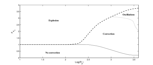
Figure 1: Numerical simulations reveal four different regions in the parameter plane $(R_{p},F_{K})$. In the lower region, there are stationary regimes without convection. In the upper region, they do not exist and solution blows up. In the intermediate region from the right, the solution remains bounded (no explosion). It can be stationary or oscillating with convection.

Convection can change conditions of heat explosion. Figure 1 shows four domains in the plane of parameters $(F_{K},R_{p})$: stationary regimes without convection, bounded (stationary or oscillating) solutions with convection, blow-up solutions (explosion).

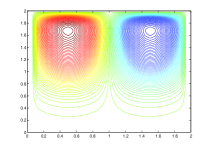
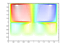
Figure 2: Stationary convective regimes. Level lines of the stream function for $F_{K}=1$, $R_{p}=100$ (left), for $F_{K}=1$, $R_{p}=1000$ (middle) and for $F_{K}=3.2$, $R_{p}=1000$ (right).

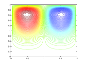
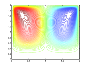
Figure 3: Stationary and Oscillating convective regimes. Level lines of the stream function for $R_{p}=3500$ and for $F_{K}=0.2$ (left), $F_{K}=1$ (middle) and for $F_{K}=3.75$ (right).

If the Rayleigh number is sufficiently small, then there is no convection and the critical value of the Frank-Kamenetskii parameter is independent of $R_{p}$. If we fix $F_{K}$ and increase $R_{p}$, then the stationary solution without convection loses its stability resulting in appearance of stationary convective regimes.

We note that convection increases heat exchange through the boundary. Therefore, the critical value of $F_{K}$, for which explosion occurs, grows when $R_{p}$ increases. If $F_{K}$ is sufficiently large, the temperature becomes unbounded, which corresponds to heat explosion. Qualitatively this diagram is similar to the case of heat explosion with convection in fluids [5, 8].

$\begin{array}[]{c}\includegraphics[scale={.43}]{psi_maxFk2_2N2}\vspace{-.3cm}\\ (a)\vspace{-.17cm}\end{array}$ $\begin{array}[]{c}\includegraphics[scale={.35}]{psi_maxFk3_7}\vspace{-.3cm}\\ (b)\vspace{-.17cm}\end{array}$

Figure 4: Oscillating convective regimes. Maximum of the stream function as a function of time for $R_{p}=4\times 10^{3}$ and for different values of $F_{K}$, $(a)F_{K}=2.2$, $(b)F_{K}=3.7$.

$\begin{array}[]{c}\includegraphics[scale={.37}]{MeanFk2}\vspace{-.3cm}\\ (a)\vspace{-.17cm}\end{array}$ $\begin{array}[]{c}\includegraphics[scale={.35}]{meanFk2_2}\vspace{-.3cm}\\ (b)\vspace{-.17cm}\end{array}$
$\begin{array}[]{c}\includegraphics[scale={.35}]{meanFk3_5}\vspace{-.3cm}\\ (c)\vspace{-.17cm}\end{array}$ $\begin{array}[]{c}\includegraphics[scale={.35}]{meanFk3_7}\vspace{-.3cm}\\ (d)\vspace{-.17cm}\end{array}$

Figure 5: Oscillating convective regimes. Mean of temperature as function of the mean value of the stream function for $R_{p}=4\times 10^{3}$ and for different values of $F_{K}$, $(a)F_{K}=2$, $(b)F_{K}=2.2$, $(c)F_{K}=3.5$, $(d)F_{K}=3.7$.

Figure $2$ shows level lines of the stream function for different values of parameters in the case of stationary convection. The maximum of the stream function grows significantly with the increase of the Rayleigh number. It is about $2\times 10^{-3}$ for $R_{p}=100$ and about $4.5$ for $R_{p}=1000$. Besides, in the second case the vortices are located closer to the upper boundary (Figure 2, left and middle). For higher values of $F_{K}$ (Figure 2, right), the maximal temperature increases, convection becomes more vigourous and there are additional four vortices located below the two main ones.

Convective patterns depend on the values of parameters. Figures $3$ show level lines of the stream function for different values of $R_{p}$ and $F_{K}$. If we put $R_{p}=3500$ and chose small Frank-Kamenetskii parameter, then we first observe two vortex regimes similar to those shown in Figure $2$. The center of the two vortex move to the corners by increasing the Frank-Kamenetskii parameter (the two first cases correspond to the stationary convective regime). For larger values of $F_{K}=3.75$, more vortices appear. They compress each other and pack vertically. This case correspond to the oscillatory convective regime.

Figure $4$ shows the maximum of the stream function as a function of time for $R_{p}=4\times 10^{3}$ and for different values of the Frank-Kamenetskii parameter. For $F_{k}>2$, instead of a stationary solution, we observe periodic oscillations. Figure $5$ shows the mean value of the temperature as a function of the mean value of the stream function. The solution forms closed curves which correspond to periodic oscillations. The structure of these curves changes with the increase of $F_{K}$. For small values, it is a simple $\infty$-shape curve. For large values, it becomes double $\infty$-shape. The transition from one to the other shown in Figure 5 b), c) where additional loops appear at upper corners. More complex structure of these curves for large $F_{K}$ canbe related to more complex convective regimes with more vortices.

If we increase the Frank-Kamenetskii parameter even more and cross the boundary separating convection and explosion domains in Figure 1, the maximum of the temperature and of the stream function oscillate during some time and then begin unlimited growth (Figure $6$). It is oscillating heat explosion similar to that found before in the case where fluid motion was described by the Navier-Stokes equations [8]. Thus, along with usual heat explosion where temperature monotonically increases, there exists oscillating heat explosion where temperature oscillates before explosion. This effect is due to the interaction of heat release and natural convection.

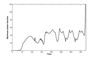
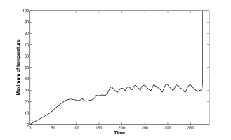
Figure 6: Maximum of the stream function (left) and of the temperature (right) as functions of time for $R_{p}=4\times 10^{3}$ and for $F_{K}=3.757$.

4 The model with non-stationary Darcy equation

4.1 The new model setting

In this section, we will consider the following model:

$$\frac{\partial T}{\partial t}+\mathbf{v}.\nabla T=\kappa\Delta T+qK(T)\phi(\alpha),$$ (4.1)

$$\frac{\partial\mathbf{v}}{\partial t}+\frac{\mu}{K}\mathbf{v}+\nabla p=g\beta\rho(T-T_{0})\mathbf{\gamma},$$ (4.2)

$$\nabla.\mathbf{v}=0.$$ (4.3)

The difference in comparison with the model studied above is that we do not consider here the quasi-stationary approximation for Darcy’s law. Introducing vorticity

$$\omega=\it{curl}\ \mathbf{v},$$ (4.4)

multiplying the equation (4.2) by $\displaystyle\frac{K}{\mu}$ and following the same steps as in Sections 2 and 3, we obtain the system of equations:

$$\frac{\partial\theta}{\partial t}+\frac{\partial\psi}{\partial y}\frac{\partial\theta}{\partial x}-\frac{\partial\psi}{\partial x}\frac{\partial\theta}{\partial y}=\frac{\partial^{2}\theta}{\partial x^{2}}+\frac{\partial^{2}\theta}{\partial y^{2}}+F_{K}e^{\theta},$$ (4.5)

$$\sigma\frac{\partial\omega}{\partial t}+\omega=R_{p}\frac{\partial\theta}{\partial x},$$ (4.6)

$$\omega=-\Delta\psi,$$ (4.7)

where the parameter $\displaystyle\sigma=\frac{1}{V_{a}}$ stands for the inverse of Vadasz number, $V_{a}=P_{r}/D_{a}$, $\displaystyle P_{r}=\frac{\mu}{\kappa}$ is the Prandtl number and $\displaystyle D_{a}=\frac{K}{\ell^{2}}$ is the Darcy number.

4.2 Numerical method and results

As before, we use the alternative direction finite difference method to solve equation (4.5) and the fast Fourier transform to solve equation (4.7). Equation (4.6) is solved by an explicit Euler method.

Figure 7 shows the mean value of the temperature as a function of the mean value of the stream function for $R_{p}=4\times 10^{3}$ and for different values of $\sigma$. When using the first model (Section 4), we obtain a small "butterfly" in the bottom of the box (cf. Figure $5$ (a)). This model is a particular case of the model introduced in Section 4.1 if we formally put $\sigma=0$. Numerical results in Figure 7 show the convergence of solutions of system (4.5)-(4.7) to the solution of system (2.6)-(2.9) as $\sigma\to 0$.

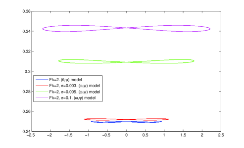
Figure 7: Mean of temperature as function of mean of stream function for $R_{p}=4\times 10^{3}$ and for different values of $\sigma$. Solution of the complete Darcy’s law converges to the solution under quasi-stationary approximation as $\sigma$ decreases.

5 Discussion

In this work, we study the influence of convection on thermal explosion in a porous medium. We begin with the model where a nonlinear reaction-diffusion equation is coupled to Darcy’s law written under the quasi-stationary approximation. Stationary and oscillating convective regimes are observed. Conditions of explosion are determined and oscillating heat explosion is found. We next consider the complete equations of motion without quasi-stationary approximation. Numerical simulations show the convergence of the solution to the solution under the quasi-stationary approximation as the Vadasz number increases.

Let us note that stationary convective regimes in the problem of heat explosion in a porous medium were already observed in literature [13], [14]. We show in this work that the structure of convective solutions depend on the intensity of heat release. When the Frank-Kamenetskii parameter increases, a second range of vortices appears in the lower part of the domain.

It is interesting that interaction of heat release with convection can result in oscillating convective regimes. Some indication to this was done in [14] where linear stability analysis showed that Hopf bifurcation could occur. The authors interpreted it as a possible transition to heat explosion and not to oscillating convective regimes. On the other hand, we have also found oscillating heat explosion where the temperature oscillates before it starts unlimited growth. Such regimes can be observed if we increase $F_{K}$ starting from periodically oscillating convective solutions.

Finally, we analyzed applicability of quasi-stationary Darcy law used in all previous works devoted to heat explosion in a porous medium. It appears that it is a good approximation for large values of the Vadasz number. However, it may not be valid for certain parameter ranges. In particular, we can expect that in some cases the quasi-stationary approximation modifies conditions of heat explosion and ignition time.

References

- [1] Semenov NN (1935) Chemical Kinetics and Chain Reactions. Clarendon Press, Oxford
- [2] Frank-Kamenetskii DA (1969) Diffusion and Heat Transfer in Chemical Kinetics. Plenum Press, New York
- [3] Zeldovich YaB, Barenblatt GI, Librovich VB, Makhviladze GM (1985) The Mathematical Theory of Combustion and Explosions. Consultants Bureau, Plenum, New York
- [4] Khudyaev SI, Shtessel EA, Pribytkova KV (1971) Numerical solution of the heat explosion problem with convection. Combustion, Explosion and Shock Waves, (Fizika goreniya i vzryva) 2:167–178
- [5] Merzhanov AS, Shtessel EA (1973) Free convection and thermal explosion in reactive systems. Astronautica Acta 18:191–193
- [6] Belk M, Volpert V (2004) Modeling of heat explosion with convection. Chaos 14:263–273
- [7] Ducrot A, Volpert V (2005) Modelling of convective heat explosion. Journal of Technical Physics 46:129–143
- [8] Dumont T, Genieys S, Massot M, Volpert V (2002) Interaction of thermal explosion and natural convection: critical conditions and new oscillating regimes. SIAM J. Appl. Math. 63:351–372
- [9] Lazarovici A, Volpert V, Merkin JH (2005) Steady states, oscillations and heat explosion in a combustion problem with convection. European Journal of Mechanics B/Fluids 24:189–203
- [10] Liu Ting-Yueh, Campbell Alasdair N, Hayhurst Allan N, Cardoso Silvana SS (2010) On the occurrence of thermal explosion in a reacting gas: The effects of natural convection and consumption of reactant. Combustion and Flame 157:230–239
- [11] Kagan L, Berestycki H, Joulin G, Sivashinsky G (1997) The effect of stirring on the limit of thermal explosion. Combustion Theory and Modelling 1:97–111
- [12] Osipov AI, Uvarov AV, Roschina NA (2007) Influence of natural convection on the parameters of thermal explosion in the horizontal cylinder. Int. J. Heat Mass Transfer 50:5226–5231
- [13] Kordilewsky W, Krajewki J (1984) Convection effects on thermal ignition in porous media. Chemical Eng. Science, 39: no. 3, 610–612.
- [14] Viljoen HJ, Hlavacek V (1987) Chemically driven convection in a porous medium. AIChE Journal 33:1344–1350
- [15] Viljoen HJ, Gatica JE, Hlavacek V (1988) Induction time for thermal explosion and natural convection in porous media. Chemical Eng. Science, 43: no. 11, 2951–2956.
- [16] Gatica JE, Viljoen HJ, Hlavacek V (1989) Interaction between chemical reaction and natural convection in porous media. Chemical Eng. Science, 44: no. 9, 1853-1870.
- [17] Balakotaiah V, Pourtalet P (1990) Natural Convection Effects on Thermal Ignition in a Porous Medium I. Semenov Model. Proc. R. Soc. Lond. A, 429: 533–554.