FRW universe in the laboratory

Abstract

We consider an expanding relativistic fluid with spherical symmetry as a model for an analog Friedmann-Robertson-Walker (FRW) spacetime. In the framework of relativistic acoustic geometry we demonstrate how to mimic an arbitrary FRW spacetime with positive, zero or negative spatial curvature. In the Lagrangian description we show that a particular FRW spacetime is obtained by choosing the appropriate potential. We discuss several examples and in particular the analog de Sitter spacetime in the coordinate representation with positive and negative spatial curvature.

1 Introduction

The possibility that a curved (pseudo-Riemannian) geometry of spacetime can be mimicked by fluid dynamics in Minkowski spacetime has been recently exploited in various contexts including emergent gravity [1], scalar theory of gravity [2], acoustic geometry [3, 4, 5] to name but a few.

The basic idea is the emergence of an effective metric of the form

$$G_{\mu\nu}=ag_{\mu\nu}+bu_{\mu}u_{\nu},$$ (1)

which describes the effective geometry for acoustic perturbations propagating in a perfect fluid potential flow with $u_{\mu}\propto\partial_{\mu}\phi$. The background spacetime metric $g_{\mu\nu}$ is usually assumed flat and the coefficients $a$ and $b$ are related to the equation of state of the fluid and the adiabatic speed of sound. Equivalently, in a field-theoretical picture the fluid velocity $u_{\mu}$ is derived from the scalar field as $u_{\mu}=\partial_{\mu}\phi/\sqrt{X}$ and $a$ and $b$ are expressed in terms of the Lagrangian and its first and second derivatives with respect to the kinetic energy term $X=g^{\mu\nu}\phi_{,\mu}\phi_{,\nu}$.

In a slightly different context, the metric of the form (1) has been used to show that a pseudo-Riemann spacetime with Lorentz signature may be derived from a Riemann metric with Euclidean signature [6, 7, 8]. In that case, the vector $u_{\mu}$ represents the normalized gradient of a hypothetical scalar field which governs the dynamics and the signature of the effective spacetime.

The effective geometry of an expanding fluid seems a promising route to model an expanding spacetime, e.g., of Friedmann-Robertson-Walker (FRW) type. However, an expanding fluid alone is not a sufficiently powerful tool for modeling an expanding spacetime of general relativity. At best, the fluid flow can be manipulated to provide a coordinate transformation to an arbitrary curved coordinate frame, with the spacetime remaining flat. For example, a boost-invariant Bjorken-type spherical expansion provides a map of the Minkowski to the Milne spacetime – a homogeneous, isotropic, expanding universe with the cosmological scale proportional to $t$ and negative spatial curvature [9].

In this paper we propose a mechanism in which the metric (1) provides a laboratory model for an analog FRW spacetime with arbitrary spatial curvature. To model an arbitrary FRW spacetime we make use of the effective acoustic geometry in which small perturbations propagate adiabatically. We show quite generally that in addition to an appropriately designed fluid expansion it is necessary to manipulate the fluid equation of state to obtain the desired geometry. By making use of a specific type of fluid expansion in Minkowski spacetime it is possible quite generally to map the Minkowski metric into spatially closed ($k=1$), open hyperbolic ($k=-1$), or open flat ($k=0$) FRW acoustic metrics. The mappings to spatially flat and hyperbolic universes have been already studied in a few specific applications, such as spatially flat analog cosmology in a non-relativistic Bose-Einstein (BE) condensate [10] and an open FRW metric in a Bjorken-like spherical expansion of a relativistic BE system [11] and of a hadronic fluid [12, 13]. We extend these ideas to a more general case that includes all three types of FRW spatial geometries. It turns out that an open FRW spacetime with zero or negative spatial curvature can be modeled in a rather straightforward way using isentropic perfect fluids such as a Bose-Einstein condensate in the Thomas-Fermi limit. The modeling of a closed FRW spacetime with positive spatial curvature requires additional assumptions.

We divide the remainder of the paper into five sections and an appendix starting with section 2, in which we give a field-theoretical description of our model. In the following section, section 3, we study the relativistic BE condensate in the context of analog cosmology. Section 4 reproduces the results of section 2 in terms of the conventional relativistic hydrodynamics. In section 5 we study the analog cosmological horizons and we present the spacetime diagrams for the analog de Sitter universe. We summarize our results and give a brief outlook in section 6. Finally, in appendix A we describe a general transformation from Minkowski to spatially curved conformal coordinates.

2 Analog spacetimes

We start with an expanding perfect fluid in Minkowski spacetime in spherical coordinates $(T,R,\vartheta,\varphi)$,

$$ds^{2}=dT^{2}-dR^{2}-R^{2}d\Omega^{2},$$ (2)

and we demand that the effective acoustic metric in comoving coordinates $(t,r,\vartheta,\varphi)$ takes the conformal FRW form with line element

$$ds^{2}=\alpha(t)^{2}\left(c_{s}^{2}dt^{2}-dr^{2}-\frac{\sin^{2}(\sqrt{k}r)}{k}d\Omega^{2}\right).$$ (3)

Here $c_{s}$ is the (generally time-dependent) speed of sound and the curvature $k$ is positive, zero, or negative for a spacetime with spherical, flat, and hyperbolic spatial geometry, respectively. To achieve this we first design the fluid flow so that it models a transformation from Minkowski to conformal coordinates $(t,r,\vartheta,\varphi)$ using the prescription of Ibison [14], which we review in appendix A. In the next section we describe the kinematics of the fluid flow suitable for modeling an FRW spacetime.

2.1 Kinematics of the flow

Applying the transformation (A.2)–(A.3), we arrive at the line element

$$ds^{2}=a^{2}(t,r)\left(dt^{2}-dr^{2}-\frac{\sin^{2}(\sqrt{k}r)}{k}d\Omega^{2}\right),$$ (4)

where $a^{2}(t,r)$ is given by (A.6). The particular choice $\gamma=\delta=1$ in (A.6) gives

$$a^{2}(t,r)=\left(\cos(\sqrt{k}r)+\cos(\sqrt{k}t)\right)^{-2}.$$ (5)

The new temporal and radial coordinates $t$ and $r$ and the spatial curvature radius $|k|^{-1/2}$ are measured in units of $m^{-1}$, where $m$ is a yet unspecified mass scale. Hence, in units of $m^{2}$ the curvature equals $k=1$, 0, or $-1$.

Since the conformal factor $a^{2}$ is a function of both $t$ and $r$, the line element (4) is generally not FRW. However, for $k=-1$, the expression for $a$ may be simplified by taking the limit $\delta\rightarrow 0$ in (A.6), in which case we obtain $a$ as a function of $t$ only,

$$a(t)=e^{\epsilon t},$$ (6)

where $\epsilon$ may take the value $+1$ or $-1$, corresponding to an expanding or collapsing universe, respectively.

The fluid which provides the desired map (A.2)–(A.3) from $(T,R)$ to $(t,r)$ coordinates is required to be at rest in $(t,r)$ coordinates. In other words the expansion of the fluid is such that the new coordinate frame $(t,r)$ is comoving, i.e., the four-velocity of the flow in the new coordinate frame is

$$u_{\mu}=(a,0,0,0),\hskip 28.45274ptu^{\mu}=(1/a,0,0,0).$$ (7)

Hence, the inverse transformation of (A.2)–(A.3) applied to (7) yields the velocity components $u_{T}$ and $u_{R}$ in the original Minkowski frame. Expressed in terms of $t$ and $r$ these components are given by (A.16) and (A.17). Specifically, for $\delta=1$ we have

$$u_{T}=\frac{1+\cos(\sqrt{k}r)\cos(\sqrt{k}t)}{\cos(\sqrt{k}r)+\cos(\sqrt{k}t)},$$ (8)

$$u_{R}=\frac{\sin(\sqrt{k}r)\sin(\sqrt{k}t)}{\cos(\sqrt{k}r)+\cos(\sqrt{k}t)}.$$ (9)

Again, for $k=-1$ we may take the limit $\delta\rightarrow 0$ and the expressions (A.16) and (A.17) reduce to

$$u_{T}=\cosh(\epsilon\,r),$$ (10)

$$u_{R}=\sinh(\epsilon\,r),$$ (11)

where $\epsilon$ equals $+1$ or $-1$, corresponding to an expanding or collapsing fluid, respectively. These velocities describe a spherically symmetric Bjorken-type expansion. This type of expansion has been recently applied to mimic an open FRW metric in a relativistic BE system [11] and in a hadronic fluid [12, 13].

The above discussed limit $\delta\rightarrow 0$ that removes the $r$-dependence of the scale factor in (4) does not work for $k=+1$ or $0$. However, as we will shortly demonstrate, with the appropriate choice of the fluid Lagrangian we can eliminate $r$-dependence even for a more general expansion of the form (8) and (9) applicable to any $k=1,0,$ or $-1$.

Next, we derive a Lagrangian that describes a fluid capable of modeling FRW spacetime in terms of the relativistic acoustic geometry.

2.2 Mapping to an analogue FRW spacetime

For our purpose it proves advantageous to use the field-theoretical description of fluid dynamics [15]. Consider a Lagrangian ${\cal L}(X,\theta)$ that depends on a dimensionless scalar field $\theta$ and on the kinetic energy term

$$X=g^{\mu\nu}{\theta}_{,\mu}\theta_{,\nu}.$$ (12)

For $X>0$, the energy-momentum tensor

$$T_{\mu\nu}=2{\cal L}_{X}\theta_{,\mu}\theta_{,\nu}-{\cal L}g_{\mu\nu},$$ (13)

takes the perfect fluid form

$$T_{\mu\nu}=(p+\rho)u_{\mu}u_{\nu}-pg_{\mu\nu},$$ (14)

in which

$$u_{\mu}=\frac{\partial_{\mu}\theta}{\sqrt{X}}.$$ (15)

Hence, the field $\theta$ serves as the velocity potential. The quantities

$$p={\cal L}\,$$ (16)

and

$$\rho=2X{\cal L}_{X}-{\cal L}$$ (17)

are identified as the pressure and energy density of the fluid, respectively, and the field equation

$$(2{\cal L}_{X}\,g^{\mu\nu}\theta_{,\mu})_{;\nu}-\partial{\cal L}/\partial\theta=0$$ (18)

is equivalent to the continuity equation. The subscript $X$ in (13)–(18) denotes a partial derivative with respect to $X$.

Small perturbations in the fluid propagate in an effective curved geometry with metric $G_{\mu\nu}$ which may be derived as follows [1, 16]. Consider a small perturbation $\chi$ around the classical solution to the field equation (18). Replacing

$$\theta(x)\rightarrow\theta(x)+\chi(x)$$ (19)

and keeping only the terms quadratic in the derivatives of $\chi$ in the Taylor expansion of the Lagrangian we obtain the effective action

$$\delta S=\frac{1}{2}\int d^{4}x\sqrt{-G}\,m^{2}G^{\mu\nu}\partial_{\mu}\chi\partial_{\nu}\chi,$$ (20)

where

$$G^{\mu\nu}=\frac{m^{2}c_{s}}{2{\cal L}_{X}}[g^{\mu\nu}-(1-\frac{1}{c_{s}^{2}})u^{\mu}u^{\nu}],$$ (21)

with $u^{\mu}=g^{\mu\nu}u_{\nu}$ and $u_{\nu}$ as defined in (15). The matrix $G^{\mu\nu}$ is the inverse of the effective metric tensor

$$G_{\mu\nu}=\frac{{2\cal L}_{X}}{m^{2}c_{s}}[g_{\mu\nu}-(1-c_{s}^{2})u_{\mu}u_{\nu}]\,,$$ (22)

with determinant $G\equiv\det G_{\mu\nu}$. The mass parameter $m$ in (20)–(22) is introduced to make $G_{\mu\nu}$ dimensionless and the quantity $c_{s}$ is the so-called “effective” speed of sound, defined as

$$c_{s}^{2}=\frac{{\cal L}_{X}}{{\cal L}_{X}+2X{\cal L}_{XX}}.$$ (23)

Hence, the linear perturbations $\chi$ propagate in the effective metric (22) and the propagation is governed by the equation of motion

$$\frac{1}{\sqrt{-G}}\partial_{\mu}\left({\sqrt{-G}}\,G^{\mu\nu}\partial_{\nu}\chi\right)+\dots=0.$$ (24)

The basic mechanism that leads to the the effective action of the form (20) with (21) was first noticed by Unruh [17] who was also the first to point out that a supersonic flow may cause analog Hawking radiation.

Due to (7) and (15), the field $\theta$ in comoving coordinates $(t,r,\vartheta,\phi)$ is a function of $t$ only and the kinetic variable $X$ is a function of both $t$ and $r$,

$$X=g^{00}\dot{\theta}^{2}=\frac{\dot{\theta}^{2}}{a^{2}},$$ (25)

where the overdot denotes a derivative with respect to $t$. The effective metric (22) in comoving coordinates takes the form

$$G_{\mu\nu}=\frac{2{\cal L}_{X}a^{2}}{m^{2}c_{s}}\left(\begin{array}[]{cccc}c_{s}^{2}&&&\\ &-1&&\\ &&-\sin^{2}(\sqrt{k}r)/k&\\ &&&-\sin^{2}\vartheta\sin^{2}(\sqrt{k}r)/k\end{array}\right).$$ (26)

A comoving observer receives information transmitted by acoustic perturbations propagating in the analog spacetime with the above effective acoustic metric.

To construct an FRW metric we must get rid of the $r$ dependence of the conformal factor, i.e., we must choose a Lagrangian with a functional dependence on $X$ such that the factor $a^{2}$ in (26) is canceled. Owing to (25) we immediately conclude that ${\cal L}_{X}$ must linearly depend on $X$ and hence our Lagrangian must be quadratic in $X$, i.e., we may choose

$${\cal L}=V(\theta)X^{2},$$ (27)

where $V$ is an arbitrary function of $\theta$. This Lagrangian belongs to a wider class of the form ${\cal L}={\cal L}(\tilde{X})$, where $\tilde{X}=f(\theta)X$ and $f(\theta)$ is an arbitrary positive function of $\theta$. By the field transformation $\tilde{\theta}_{,\mu}=f^{1/2}\theta_{,\mu}$ the variable $\tilde{X}$ becomes the kinetic term of the field $\tilde{\theta}$ and ${\cal L}(\tilde{X})$ takes the form of a purely kinetic $k$-essence which describes an isentropic fluid [18].

From (27) and using (23) we find

$$c_{s}^{2}=\frac{1}{3}.$$ (28)

A further restriction on the fluid functions $p$ and $\rho$ is imposed by the field equation (18). Applying (18) to (27) with $\theta=\theta(t)$, we obtain

$$\dot{\theta}^{3}\left(4V\ddot{\theta}+\dot{V}\dot{\theta}\right)=0.$$ (29)

By inspection it may be verified that this equation, besides the trivial solution $\theta={\rm const}$, has a solution that satisfies

$$V(\theta)\dot{\theta}^{4}=\kappa m^{4},$$ (30)

where $\kappa$ is an arbitrary dimensionless constant. Eliminating $V$ from (27) by (30) and using (16), (17), and (25) we find

$$p=\frac{\kappa m^{4}}{a^{4}},\hskip 28.45274pt\rho=\frac{3\kappa m^{4}}{a^{4}}.$$ (31)

Then, the acoustic line element corresponding to the metric (26) takes the desired form

$$ds^{2}=\alpha(\tau)^{2}\left(d\tau^{2}-dr^{2}-\frac{\sin^{2}(\sqrt{k}r)}{k}d\Omega^{2}\right),$$ (32)

where a transition to the conformal time is made by the replacement $\tau=c_{s}t$. With a convenient choice $\kappa=(c_{s}/4)^{2}$ the cosmological scale factor reads

$$\alpha(\tau)=V(\theta(\tau/c_{s}))^{1/4}.$$ (33)

In this way, we have shown that the acoustic analog metric takes the conformal form of a general FRW spacetime with positive, negative or zero spatial curvature depending on the choice of $k$ in the flow velocity (8)–(9). The evolution of the cosmological scale is determined by the shape of the potential $V$ in the Lagrangian (27).

It is instructive to study a few simple examples.

Static universe

The simplest possible case is the analog static spacetime with potential $V=1$, i.e., with the Lagrangian

$${\cal L}=X^{2}$$ (34)

It is worth noting that an effective Lagrangian of this form has been recently studied in the context of relativistic superfluidity [19]. From (30) it follows that $\theta=\kappa^{1/4}mt$. Hence, if the fluid described by the Lagrangian (34) expands according to (8)–(9) (or (10)–(11) in the $k=-1$ case), a comoving observer perceives a static open ($k=-1$) or closed ($k=1$) analog universe.

Analog de Sitter spacetime

We next consider the de Sitter (dS) geometry which admits all three representations with the corresponding line elements [14],

$$ds^{2}=\left\{\begin{array}[]{ll}\tau^{-2}(d\tau^{2}-dr^{2}-r^{2}d\Omega^{2}),&\mbox{$k=0$},\\ \cos^{-2}\tau\left(d\tau^{2}-dr^{2}-\sin^{2}rd\Omega^{2}\right),&\mbox{$k=1$},\\ \sinh^{-2}\tau\left(d\tau^{2}-dr^{2}-\sinh^{2}rd\Omega^{2}\right),&\mbox{$k=-1$}.\end{array}\right.\$$ (35)

Comparing these with (32) together with (30) and (33), we obtain $V$ and $\dot{\theta}$ as functions of $\tau$ for each $k$. Replacing $\tau=c_{s}t$ and integrating $\dot{\theta}$ over $t$, we obtain

$$4\sqrt{c_{s}}\,\theta(t)=\left\{\begin{array}[]{ll}c_{s}^{2}t^{2},&\mbox{ $k=0$},\\ 2\sin c_{s}t,&\mbox{$k=1$},\\ 2\cosh c_{s}t,&\mbox{$k=-1$}.\end{array}\right.\$$ (36)

Plugging these functions back into $V(t)$, we find

$$\ V_{\rm dS}(\theta)=\frac{\sqrt{3}}{16\theta^{2}}$$ (37)

for $k=0$ and

$$\ V_{\rm dS}(\theta)=\frac{3}{(\sqrt{3}-4\theta^{2})^{2}}$$ (38)

for both $k=1$ and $k=-1$ with the conditions $\theta^{2}<\sqrt{3}/4$ for $k=1$ and $\theta^{2}>\sqrt{3}/4$ for $k=-1$.

As demonstrated by Ibison [14], the transformation (A.2)–(A.3) with $\delta=1$, $\gamma=2$, and $k=\pm 1$ takes the dS line element in the $k=0$ representation

$$ds^{2}=\frac{1}{T^{2}}(dT^{2}-dR^{2}-R^{2}d\Omega^{2})$$ (39)

to that in the $k=\pm 1$ representations of the type (32) with

$$\alpha^{2}=\frac{k}{\sin^{2}(\sqrt{k}\tau)}.$$ (40)

Hence, the inverse coordinate transformation back to the original Minkowski coordinates takes our acoustic line element (32) with (40) to the conformal spatially flat dS line element (39), as it should because, by our construction, the acoustic metric of the fluid at rest (i.e., with $k=0$ velocity field) described by the potential (37) is $k=0$ de Sitter in the conformal form.

Analog anti–de Sitter spacetime

Anti–de Sitter (AdS) spacetime is expressible only in the $k=-1$ representation with line element [14]

$$ds^{2}=\frac{1}{\cosh^{2}\tau}\left(d\tau^{2}-dr^{2}-\frac{\sinh^{2}r}{k}d\Omega^{2}\right).$$ (41)

Repeating the above procedure, we find

$$\ V_{\rm AdS}(\theta)=\frac{3}{(\sqrt{3}+4\theta^{2})^{2}}.$$ (42)

3 Bose-Einstein condensate

In the context of relativistic acoustic geometry, an interesting example of a relativistic fluid is the BE condensate which has been suggested in a recent paper [11] as a model for an analogue FRW universe.

We first show that, under certain assumptions, self-interacting complex scalar field theories are equivalent to purely kinetic $k$-essence models (for details see [20]). We will then analyze the acoustic metric and demonstrate that an appropriately chosen $k$-essence Lagrangian can simulate arbitrary $k=0$ and $k=-1$ FRW model. As for $k=1$, purely kinetic $k$-essence Lagrangians are not suitable for the simulation of $k=-1$ FRW models except for a closed static universe, as in the first example of section 2.2.

Consider the Lagrangian

$${\cal{L}}=g^{\mu\nu}{\Phi^{*}}_{,\mu}\Phi_{,\nu}-U(|\Phi|^{2}/m^{2})$$ (43)

for a complex scalar field, where the potential $U$ is an arbitrary function of $|\Phi|^{2}/m^{2}$. The field $\Phi$ satisfies the Klein-Gordon (KG) equation

$$(g^{\mu\nu}{\Phi}_{,\nu})_{;\mu}+\frac{dU}{d|\Phi|^{2}}\Phi=0.$$ (44)

Using the representation

$$\Phi=\frac{\phi}{\sqrt{2}}\exp(-i\theta),$$ (45)

the Lagrangian (43) may be recast into the form

$${\cal{L}}=\frac{1}{2}\phi^{2}g^{\mu\nu}\theta_{,\mu}\theta_{,\mu}+\frac{1}{2}g^{\mu\nu}\phi_{,\mu}\phi_{,\nu}-U(\frac{\phi^{2}}{2m^{2}}).$$ (46)

The KG equation (44) splits into two equations for the real scalar fields $\theta$ and $\phi$,

$$(Yg^{\mu\nu}\theta_{,\nu})_{;\mu}=0,$$ (47)

$$(g^{\mu\nu}\phi_{,\nu})_{;\mu}+\phi\left(U_{Y}/m^{2}-X\right)=0,$$ (48)

where we have introduced the abbreviations

$$X=g^{\mu\nu}{\theta}_{,\mu}\theta_{,\nu}\,,\;\;\;\;\;\;Y=\frac{\phi^{2}}{2m^{2}}\,,$$ (49)

and $U_{Y}$ denotes the derivative $dU/dY$. A nontrivial classical solution to either equation (44) or equations (47)–(48) is called the relativistic Bose-Einstein condensate. The field configuration thus obtained corresponds to a two-component relativistic fluid.

The formalism of acoustic geometry is derived assuming a perfect irrotational fluid. Here, the energy-momentum tensor corresponding to the Lagrangian (43) represents a combination of two perfect fluids and generally cannot be put in the form of a single perfect fluid. However, if the spacetime variations of $|\Phi|$ are small on the scale smaller than $m^{-1}$, i.e. assuming $\phi_{,\mu}\ll m\phi$ , then the Thomas-Fermi (TF) approximation [21, 22] (or the eikonal approximation [11]) applies. In this case, if $dU/d|\Phi|^{2}>0$ the fluid becomes perfect and the corresponding Lagrangian is equivalent to a Lagrangian that depends only on the kinetic term $X$ [20]. This may be seen as follows.

The TF approximation amounts to neglecting the kinetic term $g^{\mu\nu}{\phi}_{,\mu}\phi_{,\nu}$ in (46), in which case the Lagrangian becomes

$${\cal{L}}_{\rm TF}=m^{2}XY-U(Y).$$ (50)

The field equation (47) remains the same, whereas (48) reduces to

$$m^{2}X-U_{Y}=0.$$ (51)

Now, the energy-momentum tensor corresponding to the Lagrangian (50) takes the perfect fluid form (14) with (15) and

$$\rho=YU_{Y}+U,\hskip 28.45274ptp=YU_{Y}-U.$$ (52)

Obviously, the perfect-fluid description applies only if $U_{Y}>0$ which, generally, need not be true for the entire range $0\leq Y\leq\infty$. Hence, the BE fluid in the TF approximation is perfect for those $Y$ for which $dU/d|\Phi|^{2}>0$.

Owing to (51) and the obvious relation

$${\cal{L}}_{X}=m^{2}Y,$$ (53)

equation (50) together with (51) and (53) may be interpreted as a Legendre transformation,

$${\cal L}(X)=m^{2}XY-U(Y).$$ (54)

For a given $U$ the Lagrangian ${\cal L}(X)$ can be found by solving (51) for $Y$ and plugging the solution into (54). Similarly, if ${\cal L}(X)$ is known, the potential $U$ may be derived by solving (53) for $X$ and plugging the solution into (54).

From the Lagrangian ${\cal L}(X)$ which now depends only on the kinetic term $X$ we find the equation of motion for the field $\theta$,

$$({\cal L}_{X}g^{\mu\nu}\theta_{,\nu})_{;\mu}=0,$$ (55)

which is equivalent to (47). However, one should bare in mind that the field theories described by the Lagrangians (50) and (54), respectively, are equivalent only at the classical level. The energy-momentum tensor constructed from (54) is of the form (14), with the parametric equation of state

$$\rho=2X{\cal L}_{X}-{\cal L},\hskip 28.45274ptp={\cal L}.$$ (56)

This equation is just a different parametrization of the equation of state (52) which may be easily verified by using (51) to substitute $U_{Y}$ for $X$ in (56).

In the following we study an expanding fluid in terms of the Lagrangian ${\cal L}(X)$ as a framework for an analog model of an FRW universe. As before, the effective geometry in comoving coordinates is defined by the acoustic metric (26). However, the previous procedure of eliminating $a^{2}$ in the conformal factor cannot be applied here, since ${\cal L}(X)$ is now a general function of $X$. Nevertheless, in the case of hyperbolic spatial geometry ($k=-1$) the general coordinate transformation (A.2) and (A.3) to comoving coordinates may be simplified taking the limit $\delta\rightarrow 0$. In this case the transformation (A.10)–(A.11) takes the Minkowski spacetime to the Milne spacetime with the conformal factor $a=e^{\pm t}$ being a function of $t$ only. This coordinate transformation corresponds to the Bjorken-type spherical expansion discussed already in a similar context [11, 12, 13]. In this case, $X$ is a function of $t$ only and likewise ${\cal L}_{X}$ and $c_{s}$. The effective acoustic line element in comoving coordinates,

$$ds^{2}=\frac{2{\cal L}_{X}}{m^{2}c_{s}}e^{2\epsilon t}\left(c_{s}^{2}dt^{2}-dr^{2}-\sinh^{2}rd\Omega^{2}\right)$$ (57)

can be immediately cast into the conformal FRW form for any ${\cal L}={\cal L}(X)$ by the transformation to the conformal time,

$$\tau=\int dtc_{s},$$ (58)

where $c_{s}$ is defined in (23). Therefore, by choosing an appropriate interaction potential $U$ (or equivalently, a $k$-essence Lagrangian ${\cal L}(X)$) one can, in principle, mimic the open hyperbolic FRW universe of arbitrary kind. This procedure, albeit straightforward, is slightly more involved than the one explained in section 2 because the speed of sound is generally not constant.

Given a $k$-essence Lagrangian ${\cal L}(X)$ it is relatively easy to find the corresponding analog FRW spacetime. First, from the field equation (55) we find the relation

$${\cal L}_{X}=m^{3}e^{-3\epsilon t}X^{-1/2},$$ (59)

from which we can express $X$, ${\cal L}(X)$, and $c_{s}$ in terms of $t$. These in turn yield a functional dependence on $t$ of the conformal factor

$$\alpha^{2}\equiv\frac{2{\cal L}_{X}}{m^{2}c_{s}}e^{2\epsilon t}$$ (60)

in the line element (57). Then, using (23) and (58), we find $t$ as a function of the conformal time $\tau$, which in turn yields $\alpha=\alpha(\tau)$.

The reverse procedure is slightly more involved. Suppose we want to model a particular hyperbolic FRW spacetime of the form

$$ds^{2}=\alpha(\tau)^{2}\left(d\tau^{2}-dr^{2}-\sinh^{2}rd\Omega^{2}\right).$$ (61)

We need to find the Lagrangian $\cal{L}$ such that the conformal factor of the corresponding acoustic line element (57) is equal to $\alpha(\tau)$, i.e, we require (60). First, from (59) and using (23), we find

$$c_{s}^{2}=-\frac{\epsilon}{6X}\frac{dX}{dt}.$$ (62)

From this, with (60) and $d\tau=c_{s}dt$, we obtain two coupled differential equations,

$$\frac{dt}{d\tau}=\left(\frac{X}{m}\right)^{1/2}e^{\epsilon t}\alpha(\tau)^{2},$$ (63)

$$\frac{1}{X}\frac{dX}{d\tau}=-6\epsilon\left(\frac{dt}{d\tau}\right)^{-1},$$ (64)

the solution to which yields $t$ as a function of $X$ in a parametric form. This function can, in principle, be made explicit by eliminating the parameter $\tau$. Plugging $t(X)$ into (59), we obtain ${\cal L}_{X}$ as a function of $X$ from which we find ${\cal L}(X)=\int dX{\cal L}_{X}(X)$.

We consider two examples, one for each procedure discussed above.

Scalar Born-Infeld theory

As an easily tractable example, consider the BE interaction potential

$$U=m^{4}(Y^{2}+Y^{-2}),$$ (65)

which, in the Thomas-Fermi limit, is equivalent to the scalar Born-Infeld theory with the $k$-essence type Lagrangian [20, 23]

$${\cal L}=-m^{4}\sqrt{1-X/m^{2}}.$$ (66)

This theory is based on the dynamics of a $d$-brane in the $d+1$-dimensional bulk [24, 25] and is of particular interest in cosmology because of its potential for unifying dark energy and dark matter in a single entity called the Chaplygin gas [23, 26, 27, 28]. Using the relation (59), the speed of sound can be expressed as

$$c_{s}=(1-X/m^{2})^{1/2}=\left(1+e^{-6\epsilon t}\right)^{-1/2}.$$ (67)

From this we find the relation between $t$ and the conformal time $\tau$

$$e^{3\epsilon t}=\sinh 3\epsilon\tau,$$ (68)

which may be used to express $X$, ${\cal L}(X)$, and $c_{s}$ in terms of $\tau$. Then, using (60), one finds

$$\alpha(\tau)=(\sinh 3\epsilon\tau)^{-2/3}\cosh 3\epsilon\tau.$$ (69)

Exponential expansion

As an example of the inverse problem that can be solved analytically, consider the scale factor in the form of an exponential function,

$$\alpha(\tau)=e^{\beta\tau}.$$ (70)

Equations (63) and (64) can be solved by the ansatz

$$\left(\frac{X}{m}\right)^{1/2}e^{\epsilon t}\alpha(\tau)^{2}={\rm const}\equiv 1/c_{s}.$$ (71)

One easily finds that the Lagrangian is of the form

$${\cal L}=m^{4-2\eta}X^{\eta},$$ (72)

where the power $\eta$ satisfies

$$(\eta-2)^{2}-\beta^{2}(2\eta-1)=0,$$ (73)

and the speed of sound is given by

$$c^{2}=(2\eta-1)^{-1}.$$ (74)

Obviously, physical solutions must satisfy $\eta\geq 1$. The Milne universe ($\beta=\pm 1$) is obtained with $\eta=1$ and $\eta=5$ and the static hyperbolic universe ($\beta=0$) with $\eta=2$. The Lagrangian (72) with $\eta=2$ belongs to the class discussed in section 2 and may also be used to mimic a static closed universe ($k=1$) with the help of the expansion (8)–(9).

4 Hydrodynamic picture

Now we move from the field-theoretical description of fluid dynamics to the standard relativistic hydrodynamic formalism to demonstrate less formally and perhaps more convincingly that an expanding fluid in Minkowski spacetime can be mapped into an analog FRW spacetime of any spatial curvature.

First we note that if we identify the particle number density as

$$n=2\sqrt{X}{\cal L}_{X}.$$ (75)

and the specific enthalpy as

$$w=\frac{p+\rho}{n}=\sqrt{X}$$ (76)

the effective metric (26) takes the form

$$G_{\mu\nu}=\frac{n}{m^{2}wc_{s}}[g_{\mu\nu}-(1-c_{s}^{2})u_{\mu}u_{\nu}]$$ (77)

which, up to the normalization factor $1/m^{2}$, equals the acoustic metric derived in Ref. [4] for a perfect fluid potential flow with velocity given by

$$wu_{\mu}=\partial_{\mu}\theta$$ (78)

and the adiabatic speed of sound $c_{s}$ defined as

$$c_{s}^{2}=\left.\frac{dp}{d\rho}\right|_{s/n}.$$ (79)

It may be shown [29] that this definition of the speed of sound coincides with the definition (23) of the effective speed of sound.

As before, the velocity potential $\theta$ in comoving coordinates $(t,r)$ is a function of $t$ only and hence

$$wu_{0}=wa=\dot{\theta}.$$ (80)

Thus, the acoustic line element in comoving coordinates reads

$$ds^{2}=\frac{na^{3}}{m^{2}c_{s}\dot{\theta}}\left(c_{s}^{2}dt^{2}-dr^{2}-\frac{\sin^{2}(\sqrt{k}r)}{k}d\Omega^{2}\right).$$ (81)

Our aim is to make the above line element FRW, i.e., to design a fluid for which the conformal factor and the speed of sound are functions of $t$ only. For this purpose, we prove that the speed of sound $c_{s}$ and the conformal factor in (81) will not depend on $r$ if and only if the particle number density is a function of $t$ and $r$ of the form

$$n=\frac{m^{3}}{a^{3}}f(t),$$ (82)

where $f(t)$ is an arbitrary dimensionless function of $t$.

First, suppose $c_{s}$ and the conformal factor are functions of $t$ only. Then, it follows immediately that $n$ is of the form (82) with $f=c_{s}\dot{\theta}/m$. To prove the reverse, suppose Eq. (82) holds. Then clearly, the conformal factor will not depend on $r$ if $c_{s}$ does not depend on $r$. Hence, it is sufficient to show that $c_{s}$ is independent of $r$. First we note that

$$p+\rho=wn=\frac{m^{3}}{a^{4}}f(t)\dot{\theta},$$ (83)

as a consequence of (80) and (82). This in turn implies that the pressure and density are generally of the form

$$p=\frac{f_{p}(t)}{a^{4}}+\chi(t,a),\hskip 28.45274pt\rho=\frac{f_{\rho}(t)}{a^{4}}-\chi(t,a),$$ (84)

where $\chi$ is yet unknown function of $t$ and $a$, and $f_{p}$ and $f_{\rho}$ are functions of $t$ such that

$$f_{p}+f_{\rho}=m^{3}f(t)\dot{\theta}.$$ (85)

The function $\chi$ is not arbitrary since $p$ and $\rho$ must satisfy the continuity equation

$$u^{\mu}\rho_{,\mu}+(p+\rho){u^{\mu}}_{;\mu}=0,$$ (86)

which follows from the energy-momentum conservation. We now demonstrate that $\chi$ is of the form $\chi=g(t)/a^{4}$ where $g(t)$ is a function that does not depend on $r$. Using (7) and (84), the continuity equation (86) may be written as

$$\dot{\chi}=\frac{\dot{f}_{\rho}}{a^{4}}+(3f_{p}-f_{\rho})\frac{\dot{a}}{a^{5}}.$$ (87)

Comparing this with the general expression for the time derivative of $\chi$,

$$\dot{\chi}=\frac{\partial\chi}{\partial t}+\frac{\partial\chi}{\partial a}\dot{a},$$ (88)

we have

$$\frac{\partial\chi}{\partial t}=\frac{\dot{f}_{\rho}}{a^{4}},\hskip 28.45274pt\frac{\partial\chi}{\partial a}=\frac{3f_{p}-f_{\rho}}{a^{5}}.$$ (89)

These two equations have a unique solution,

$$\chi=-\frac{3f_{p}-f_{\rho}}{4a^{4}},$$ (90)

and hence $\chi$ is indeed of the form $g(t)/a^{4}$. Furthermore, from (84) and (90) it follows that $c_{s}^{2}=p/\rho=1/3$, and hence $c_{s}$ is independent of $r$, which was to be shown.

Without loss of generality, we may set $\chi\equiv 0$ in (84), in which case equation (89) implies

$$3f_{p}-f_{\rho}=0,\hskip 28.45274pt\dot{f}_{\rho}=0,$$ (91)

yielding the previously obtained expressions for the pressure and density (31), where $\kappa$ is an arbitrary positive dimensionless constant. Equations (31) provide a relation between the functions $f(t)$ and $\dot{\theta}$. From (31) and (83) we find $\dot{\theta}=4\kappa m/f(t)$. Our fluid is then specified by (82) and (31). Furthermore, if we identify $f(t)=4\kappa^{3/4}V^{1/4}$ and choose $\kappa=(c_{s}/4)^{2}$ as before, the acoustic line element (81) takes precisely the same conformal FRW form (32) with (33). The evolution of the cosmological scale is determined by the function $f(t)$ that appears in the expression (82) for the particle number density.

5 Analog horizons

In this section we derive the expressions for the Hubble and the apparent horizons for a general analog FRW spacetime such as that in sections 2 and 4. The FRW line element considered here is assumed to be in the conformal form (32), with the acoustic conformal time $\tau=c_{s}t$. The proper distance $d_{\rm p}$ and the comoving spatial distance $r$ are related by $d_{\rm p}=\alpha r$ as usual, whereas the analog Hubble expansion rate in conformal coordinates is given by

$${\cal H}=\frac{\dot{\alpha}}{\alpha^{2}},$$ (92)

where the overdot denotes a partial derivative with respect to $\tau$. We define the analog Hubble horizon as a two-dimensional spherical surface at which the magnitude of the analog recession velocity

$$v_{\rm rec}\equiv{\cal H}d_{\rm p}=r\frac{\dot{\alpha}}{\alpha}$$ (93)

equals the maximally allowed velocity of sound, $c_{s}=1$. Hence, the condition

$$r=\frac{\alpha}{\left|\dot{\alpha}\right|}$$ (94)

defines the location of the analog Hubble horizon.

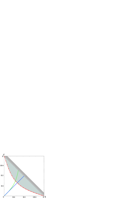
Figure 1: Spacetime diagram of the analog $k=1$ dS spacetime in $(\tau,r)$ coordinates. The evolution of the apparent, Hubble, and naive horizons are represented by the full, dashed, and dash-dotted lines, respectively. The shaded area represents the region in which $v\geq c_{s}$. The diagonal “wall” marks the boundary of the physical region.

Next we define the analog apparent horizon as a boundary of the analog trapped region [13]. More precisely, the apparent horizon is defined as a two-dimensional surface on which one of the null expansions vanishes [30]. In the case of spherical symmetry one can use a more practical definition: the apparent horizon is a two-dimensional surface $H$ such that the vector $n_{\mu}$, normal to the surface of spherical symmetry is null on $H$. In our case it means that $n_{\mu}$ is null with respect to the acoustic metric. More explicitly, the acoustic metric magnitude of the vector

$$n_{\mu}=\partial_{\mu}(\alpha\sin(\sqrt{k}r)/\sqrt{k})$$ (95)

should be zero on $H$ , i.e.,

$$G^{\mu\nu}n_{\mu}n_{\nu}|_{H}=0.$$ (96)

From this one finds the condition for the apparent horizon

$$\frac{\dot{\alpha}}{\alpha}\pm\sqrt{k}\cot(\sqrt{k}r)=0,$$ (97)

where $k=1,-1$. Any solution to Eq. (97) gives the location of the analog apparent horizon $r_{H}$.

Finally, we define the naive horizon as a two-dimensional surface on which the radial velocity $v\equiv u_{R}/u_{T}$ equals the velocity of sound $c_{s}$. In the case of a stationary spherically symmetric flow, the apparent and naive horizons coincide with the analog event horizon [3].

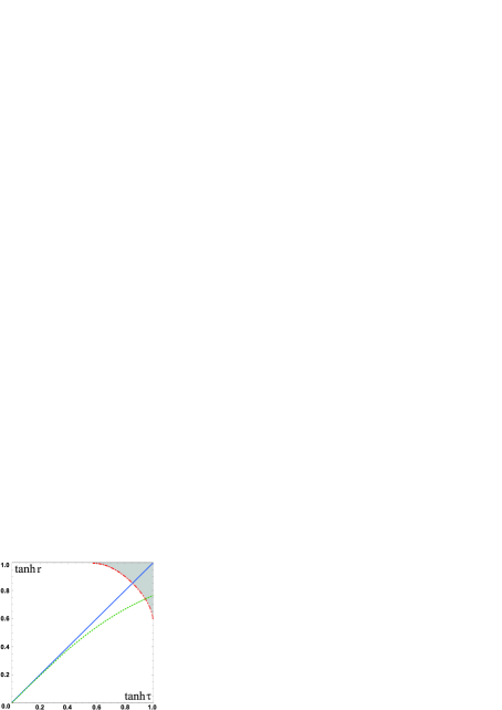
Figure 2: Spacetime diagram of the $k=-1$ analog dS spacetime. The evolution of the apparent, Hubble, and naive horizons are represented by the full, dashed, and dash-dotted lines, respectively.

As a simple example, we consider the analog de Sitter spacetime with positive or negative spatial curvature. We have shown in section 2 how to mimic the $k=1$ and $k=-1$ representations of the dS spacetime: the fluid described by the Lagrangian (27) with the potential (38) should be forced to expand according to (8)–(9) where $k$ determines whether the analog spacetime has a positive or negative curvature. In Figs. 1 and 2 we plot the spacetime diagrams in conformal coordinates $(\tau,r)$ for the analog dS universe with positive and negative spatial curvature, respectively. The diagrams depict the evolution of the apparent (full line), analog (dashed line), and naive Hubble (dash-dotted line) horizons. The shaded area in both figures represents the region of supersonic flow, i.e., the region in which the fluid three-velocity $v$ exceeds the speed of sound $c_{s}$. The diagonal line $t+r=\pi$ in Fig. 1 corresponds to the future infinity, i.e., the point $R=T=\infty$ in Minkowski coordinates.

6 Discussion and conclusions

We have demonstrated that it is possible, at least in principle, to model an FRW spacetime with arbitrary spatial curvature using a relativistic fluid and the associated effective acoustic geometry. To obtain the desired geometry one needs to manipulate the fluid equation of state in addition to an appropriately designed fluid expansion. We have shown in section 3 that an open FRW spacetime with zero or negative spatial curvature can be modeled using isentropic perfect fluids such as a Bose-Einstein condensate in the Thomas-Fermi limit. The modeling of a closed FRW spacetime with positive spatial curvature is possible if the condition of isentropy is relaxed. This is achieved by a Lagrangian with a quadratic kinetic energy term multiplied by a potential $V,$ the choice of which determines the evolution of the analog cosmological scale. The acoustic analog metric takes the conformal form of a general FRW spacetime with positive, negative, or zero spatial curvature depending on the choice of the sign parameter $k$ in the expression (8)–(9) for the flow velocity.

It is conceivable that the analysis presented here is of considerable theoretical interest for emergent gravity models, in particular for those in which the emergent gravity is based on fluid flow (for a comprehensive review and extensive list of references, see Ref. [31]). It is worth mentioning a few examples in which there is an obvious connection to our analysis. The first one concerns already mentioned emergence of scalar gravity. As was shown in Ref. [32], in the framework of the fluid-field correspondence one can go beyond analog gravity by introducing a scalar field Lagrangian that describes the dynamics of a scalar field as an interaction of the field and its associated effective metric given by (22). This interaction may be interpreted as a gravitational influence on the field by its own effective metric [2, 32]. Another example is the model of Janik and Peschanski [33] in which perfect fluid hydrodynamics emerges as a consequence of the AdS/CFT correspondence. In their approach the AdS/CFT correspondence relates a perfect conformal fluid on the boundary to an asymptotically AdS₅ bulk. The link to our study is twofold: first, the fluid described by the Lagrangian (27) is conformal and second, the longitudinal Bjorken expansion of Ref. [33] is of the same form as our spherical expansion (10) and (11) obtained from the more general expression in the limit when the parameter $\delta$ approaches zero. Assuming a true AdS/CFT duality, the boundary conformal fluid in the model of Ref. [33] may also be regarded as primary and the bulk as emergent [34].

In our study so far we have discussed simple toy models with no realistic fluid in mind. To the best of our knowledge, the only realistic experimental set up for a relativistic-fluid laboratory is provided by high-energy colliders. In our previous papers [12, 13] we suggested a relativistic collision model based on a spherical Bjorken-type expansion to mimic an open FRW universe. To model a closed universe, a different type of expansion is needed with the $k=1$ velocity field (8)–(9). Presently we do not have a concrete proposal for how to do this in high-energy collisions. Maybe, with the advance of accelerator technology, one day it will be possible, e.g., by choosing appropriate heavy ions and specially designed beam geometry to obtain the desired equation of state and expansion flow of the fluid. To confront the model with experiment and test the properties of the analog spacetime it would be of interest to investigate the effects of the cosmological particle production in our relativistic model in the same way as it was done in the nonrelativistic analog models of expanding universes [35, 36]. Besides, the presence of a trapped region and the apparent horizon can, in principle, be detected by looking for a signal of the analog Hawking radiation in the particle distribution spectra.

Acknowledgments

This work was supported by the Ministry of Science, Education and Sport of the Republic of Croatia under Contract No. 098-0982930-2864 and partially supported by the ICTP-SEENET-MTP grant PRJ-09 “Strings and Cosmology” in the frame of the SEENET-MTP Network. N. B. thanks CNPq, Brazil, for partial support and the University of Juiz de Fora where a part of this work has been completed.

Appendix A Transformations to conformal coordinates

Here we describe the procedure [14] for a transformation from Minkowski spherical coordinates to conformal spatially closed or hyperbolic coordinates. We start from the background spacetime of the form

$$ds^{2}=dT^{2}-dR^{2}-R^{2}d\Omega^{2},$$ (A.1)

and apply the following transformation:

$$T(t,r)=T_{0}+\frac{\gamma}{2\delta^{2}\sqrt{-k}}\left[f(t+r)+f(t-r)\right],$$ (A.2)

$$R(t,r)=R_{0}+\frac{\gamma}{2\delta^{2}\sqrt{-k}}\left[f(t+r)-f(t-r)\right],$$ (A.3)

where

$$f(x)=\tanh\left(\frac{\sqrt{-k}}{2}x+\log\delta\right),$$ (A.4)

$T_{0}$, $R_{0}$, $\gamma$, and $\delta$ are constants, and $k=1,0,-1$ for the spherical, flat, or hyperbolic spatial geometry, respectively. Without loss of generality the offsets $T_{0}$, $R_{0}$, to the origins of $T$ and $R$ may be set to zero with the implicit assumption that in any result the coordinates $T$ and $R$ can be linearly rescaled. This transformation takes the line element (A.1) to the conformal form

$$ds^{2}=a^{2}(t,r)\left(dt^{2}-dr^{2}-\frac{\sin^{2}(\sqrt{k}r)}{k}d\Omega^{2}\right),$$ (A.5)

where

$$a^{2}(t,r)=\frac{\gamma^{2}}{\delta^{4}\left[\cosh(\sqrt{-k}r)+\cosh(\sqrt{-k}t+2\log\delta)\right]^{2}},$$ (A.6)

or equivalently, in terms of $T$ and $R$,

$$\ a^{2}(T,R)=\left[\frac{\gamma}{2\delta^{2}}-\frac{\delta^{2}}{2\gamma}k(T^{2}-R^{2})\right]^{2}+kT^{2}.$$ (A.7)

These expressions can be simplified by a convenient choice of the constants $\gamma$ and $\delta$. Specifically, for $\gamma=2$ and $\delta=1$ we obtain

$$\ a^{2}(t,r)=\left\{\begin{array}[]{ll}1,&\mbox{$k=0$};\\ 4/(\cos r+\cos t)^{2},&\mbox{ $k=+1$};\\ 4/(\cosh r+\cosh t)^{2},&\mbox{$k=-1$},\end{array}\right.\$$ (A.8)

$$\ a^{2}(T,R)=\left\{\begin{array}[]{ll}1,&\mbox{$k=0$};\\ \left[1-(T^{2}-R^{2})/4\right]^{2}+T^{2},&\mbox{$k=+1$};\\ \left[1+(T^{2}-R^{2})/4\right]^{2}-T^{2},&\mbox{$k=-1$}.\end{array}\right.\$$ (A.9)

A particularly simple transformation is obtained in the limit $\delta\rightarrow 0$ in which case one must choose a nonzero offset $T_{0}$ in (A.2) to obtain a finite result. In this limit the transformation (A.2)–(A.4) with $T_{0}=\gamma/(\delta^{2}\sqrt{-k})$ takes the form

$$T=2\gamma\frac{e^{\sqrt{-k}t}}{\sqrt{-k}}\cosh(\sqrt{-k}r),$$ (A.10)

$$R=2\gamma\frac{e^{\sqrt{-k}t}}{\sqrt{-k}}\sinh(\sqrt{-k}r),$$ (A.11)

which, obviously, makes sense only for $k=-1$. Then we obtain the conformal representation of the Milne universe,

$$ds^{2}=e^{2\epsilon t}\left(dt^{2}-dr^{2}-\sinh^{2}rd\Omega^{2}\right)$$ (A.12)

where $\epsilon$ may take the value $+1$ or $-1$, corresponding to an expanding or collapsing universe, respectively. This is the only possible nontrivial map from the Minkowski spacetime to an FRW spacetime with negative spatial curvature. A direct map to an FRW space with positive spatial curvature is not possible with the coordinate transformation (A.2).

Consider next a spherically expanding (or contracting) fluid such that the $(t,r)$ coordinate frame is comoving, i.e., such that the flow velocity of the expanding fluid in that frame is

$$u_{\mu}=(a,0,0,0).$$ (A.13)

Then, the components of the velocity in the $(T,R)$ coordinate frame are

$$u_{T}=g_{00}^{-1/2}T_{,t},$$ (A.14)

$$u_{R}=g_{00}^{-1/2}R_{,t}.$$ (A.15)

Using this and (A.2)–(A.4), we find the velocity components expressed in terms of $t$ and $r$,

$$u_{T}=\frac{2\delta^{2}+\cosh(\sqrt{-k}r)\left(e^{-\sqrt{-k}t}+e^{\sqrt{-k}t}\delta^{4}\right)}{2\delta^{2}\cosh(-\sqrt{k}r)+e^{-\sqrt{-k}t}+e^{\sqrt{-k}t}\delta^{4}},$$ (A.16)

$$u_{R}=\frac{\sinh(\sqrt{-k}r)\left(e^{-\sqrt{-k}t}-e^{\sqrt{-k}t}\delta^{4}\right)}{2\delta^{2}\cosh(-\sqrt{k}r)+e^{-\sqrt{-k}t}+e^{\sqrt{-k}t}\delta^{4}}.$$ (A.17)

and in terms of $T$ and $R$,

$$u_{T}=\frac{1}{a(T,R)}\left[\frac{\gamma}{2\delta^{2}}+\frac{\delta^{2}}{2\gamma}k(T^{2}+R^{2})\right]$$ (A.18)

$$u_{R}=\frac{1}{a(T,R)}\frac{\delta^{2}}{\gamma}kTR,$$ (A.19)

where $a(T,R)$ is given by (A.7).

References

- [1] E. Babichev, V. Mukhanov, and A. Vikman, “k-Essence, superluminal propagation, causality and emergent geometry,” JHEP 0802, 101 (2008) [arXiv:0708.0561 [hep-th]].
- [2] M. Novello, E. Bittencourt, U. Moschella, E. Goulart, J. M. Salim, and J. D. Toniato, “Geometric scalar theory of gravity,” JCAP 1306, 014 (2013) [arXiv:1212.0770 [gr-qc]].
- [3] M. Visser, “Acoustic black holes: horizons, ergospheres, and Hawking radiation”, Class. Quant. Grav. 15, 1767 (1998) [arXiv:gr-qc/9712010].
- [4] N. Bilić, “Relativistic Acoustic Geometry,” Class. Quant. Grav. 16, 3953 (1999) [arXiv:gr-qc/9908002].
- [5] S. Kinoshita, Y. Sendouda, and K. Takahashi, “Acoustic causality in relativistic shells,” Phys. Rev. D 70, 123006 (2004). [astro-ph/0405149].
- [6] J. F. Barbero G., “From Euclidean to Lorentzian General Relativity: The Real Way,” Phys. Rev. D 54, 1492 (1996) [arXiv:gr-qc/9605066].
- [7] J. F. Barbero G. and E. J. S. Villasenor, “Lorentz Violations and Euclidean Signature Metrics,” Phys. Rev. D 68, 087501 (2003) [gr-qc/0307066].
- [8] S. Mukohyama and J. P. Uzan, “From configuration to dynamics – Emergence of Lorentz signature in classical field theory,” Phys. Rev. D 87, 065020 (2013) [arXiv:1301.1361 [hep-th]].
- [9] M. A. Lampert, J. F. Dawson, and F. Cooper, “Time evolution of the chiral phase transition during a spherical expansion,” Phys. Rev. D 54, 2213 (1996) [hep-th/9603068]; G. Amelino-Camelia, J. D. Bjorken, and S. E. Larsson, “Pion production from baked Alaska disoriented chiral condensate,” Phys. Rev. D 56, 6942 (1997); M. A. Lampert and C. Molina-Paris, “Effective equation of state for a spherically expanding pion plasma,” Phys. Rev. D 57, 83 (1998).
- [10] C. Barcelo, S. Liberati, and M. Visser, “Analog gravity from Bose-Einstein condensates,” Class. Quant. Grav. 18, 1137 (2001) [gr-qc/0011026].
- [11] S. Fagnocchi, S. Finazzi, S. Liberati, M. Kormos, and A. Trombettoni, “Relativistic Bose-Einstein Condensates: a New System for Analogue Models of Gravity,” New J. Phys. 12, 095012 (2010) [arXiv:1001.1044 [gr-qc]].
- [12] N. Bilić and D. Tolić, “Analogue surface gravity near the QCD chiral phase transition,” Phys. Lett. B 718, 223 (2012) [arXiv:1207.2869 [hep-th]].
- [13] N. Bilić and D. Tolić, “Trapped surfaces in a hadronic fluid,” Phys. Rev. D 87, 044033 (2013) [arXiv:1210.3824 [gr-qc]].
- [14] M. Ibison, “On the conformal forms of the Robertson-Walker metric,” J. Math. Phys. 48, 122501 (2007) [arXiv:0704.2788 [gr-qc]].
- [15] J. Garriga and V.F. Mukhanov, “Perturbations in k-inflation,” Phys. Lett. B 458, 219 (1999).
- [16] J.U. Kang, V. Vanchurin, and S. Winitzki, “Attractor scenarios and superluminal signals in k-essence cosmology,” Phys. Rev. D 76, 083511 (2007).
- [17] W. Unruh, “Experimental Black-Hole Evaporation,” Phys. Rev. Lett. 46, 1351 (1981).
- [18] O. F. Piattella, J. C. Fabris, and N. Bilić, “Note on the thermodynamics and the speed of sound of a scalar field,” arXiv:1309.4282 [gr-qc].
- [19] M. Mannarelli and C. Manuel, “Transport theory for cold relativistic superfluids from an analogue model of gravity,” Phys. Rev. D 77, 103014 (2008) [arXiv:0802.0321 [hep-ph]].
- [20] N. Bilić, “Thermodynamics of dark energy,” Fortschr. Phys. 56, 363 (2008) [arXiv:0812.5050 [gr-qc]]; N. Bilić, “Thermodynamics of k-essence,” Phys. Rev. D 78, 105012 (2008) [arXiv:0806.0642 [gr-qc]].
- [21] D. Jaksch, C.W. Gardiner, K.M. Gheri, and P. Zoller, “Quantum kinetic theory IV: Intensity and amplitude fluctuations of a Bose- Einstein condensate at finite temperature including trap loss”, Phys. Rev. A 58, 1450 (1998).
- [22] A.S. Parkins and D.F. Walls, “The physics of trapped dilute-gas Bose-Einstein condensates,” Phys. Rep. 303, 1 (1998).
- [23] N. Bilić, G.B. Tupper, and R.D. Viollier, “Unification of Dark Matter and Dark Energy: the Inhomogeneous Chaplygin Gas,” Phys. Lett. B535, 17 (2002) [astro-ph/0111325].
- [24] R. Jackiw, Lectures on fluid dynamics. A Particle theorist’s view of supersymmetric, non-Abelian, noncommutative fluid mechanics and d-branes (Springer-Verlag, New-York, 2002).
- [25] N. Bilić, G. B. Tupper, and R. D. Viollier, “Chaplygin Gas Cosmology: Unification of Dark Matter and Dark Energy,” J. Phys. A 40, 6877 (2007) [gr-qc/0610104].
- [26] A. Kamenshchik, U. Moschella, and V. Pasquier, “An alternative to quintessence,” Phys. Lett. B 511, 265 (2001).
- [27] J. C. Fabris, S. V. B. Gonçalves, and P. E. de Souza, “Density perturbations in an Universe dominated by the Chaplygin gas,” Gen. Rel. Grav. 34, 53 (2002); “Mass Power Spectrum in a Universe Dominated by the Chaplygin Gas,” Gen. Rel. Grav. 34, 2111 (2002).
- [28] M. C. Bento, O. Bertolami, and A. A. Sen, “Generalized Chaplygin gas, accelerated expansion and dark energy-matter unification,” Phys. Rev. D 66, 043507 (2002) [arXiv:gr-qc/0202064].
- [29] N. Bilić, G. B. Tupper, and R. D. Viollier, “Cosmological tachyon condensation,” Phys. Rev. D 80, 023515 (2009) [arXiv:0809.0375 [gr-qc]].
- [30] S. A. Hayward, “General laws of black hole dynamics,” Phys. Rev. D 49, 6467 (1994).
- [31] C. Barcelo, S. Liberati, and M. Visser, “Analogue gravity,” Living Rev. Rel. 8, 12 (2005) [Living Rev. Rel. 14, 3 (2011)], [gr-qc/0505065].
- [32] M. Novello and E. Goulart, “Beyond Analog Gravity: The Case of Exceptional Dynamics,” Class. Quant. Grav. 28, 145022 (2011) [arXiv:1102.1913 [gr-qc]].
- [33] R. A. Janik and R. B. Peschanski, “Asymptotic perfect fluid dynamics as a consequence of Ads/CFT,” Phys. Rev. D 73, 045013 (2006) [hep-th/0512162].
- [34] S. Carlip, “Challenges for Emergent Gravity,” arXiv:1207.2504 [gr-qc].
- [35] C. Barcelo, S. Liberati, and M. Visser, “Probing semiclassical analog gravity in Bose-Einstein condensates with widely tunable interactions,” Phys. Rev. A 68, 053613 (2003) [arXiv:cond-mat/0307491].
- [36] S. Weinfurtner, P. Jain, M. Visser, and C. W. Gardiner, “Cosmological particle production in emergent rainbow spacetimes,” Class. Quant. Grav. 26, 065012 (2009) [arXiv:0801.2673 [gr-qc]].