Collective behavior of penetrable self-propelled rods in two dimensions
Abstract
Collective behavior of self-propelled particles is observed on a microscale for swimmers such as sperm and bacteria as well as for protein filaments in motility assays. The properties of such systems depend both on their dimensionality and the interactions between their particles. We introduce a model for self-propelled rods in two dimensions that interact via a separation-shifted Lennard-Jones potential. Due to the finite potential barrier, the rods are able to cross. This model allows us to efficiently simulate systems of self-propelled rods that effectively move in two dimensions but can occasionally escape to the third dimension in order to pass each other. Our quasi-two-dimensional self-propelled particles describe a class of active systems that encompasses microswimmers close to a wall and filaments propelled on a substrate. Using Monte Carlo simulations, we first determine the isotropic-nematic transition for passive rods. Using Brownian dynamics simulations, we characterize cluster formation of self-propelled rods as a function of propulsion strength, noise, and energy barrier. Contrary to rods with an infinite potential barrier, an increase of the propulsion strength does not only favor alignment but also effectively decreases the potential barrier that prevents crossing of rods. We thus find a clustering window with a maximum cluster size at medium propulsion strengths.
pacs:
82.70.–y, 47.63.Gd, 87.18.Hf, 64.70.M–I Introduction
Collective behavior of active bodies is frequently found in macroscopic systems such as bird flocks and fish schools Vicsek and Zafeiris (2012), but also is found in microscopic systems such as sperm cells Riedel et al. (2005); Yang et al. (2008), bacteria Ben-Jacob et al. (2000); Sokolov et al. (2007); Peruani et al. (2012); Gachelin et al. (2013), and manmade microswimmers that propel themselves forward using a chemical or physical mechanism Paxton et al. (2004); Volpe et al. (2011); Mei et al. (2011); Ebbens et al. (2012); Yang and Ripoll (2011). Despite the different natures of these systems, they all exhibit interactions that favor alignment of neighboring bodies, thus leading to similar forms of collective behavior. Of particular interest for us are experiments with elongated self-propelled particles on the microscopic scale in two dimensions, such as motility assays where actin filaments are propelled on a carpet of myosin motor proteins Harada et al. (1987); Schaller et al. (2010), microtubules propelled by surface-bound dyneins Sumino et al. (2012), and microswimmers that are attracted to surfaces Lauga et al. (2006); Berke et al. (2008); Elgeti and Gompper (2009); Elgeti et al. (2010); Elgeti and Gompper (2013).
In the pioneering work of Vicsek et al. Vicsek et al. (1995), nonequilibrium phase transitions were observed for systems with self-propelled point particles that interact via an imposed alignment rule and thermal noise. This work led to numerous analytical Toner and Tu (1995); Simha and Ramaswamy (2002); Ramaswamy et al. (2003); Toner et al. (2005); Peruani et al. (2008); Bertin et al. (2009); Golestanian (2009) as well as computational Redner et al. (2013); Szabó et al. (2006); Grégoire and Chaté (2004); Huepe and Aldana (2004); D’Orsogna et al. (2006); Aldana et al. (2007); Chaté et al. (2008); Ginelli et al. (2010) studies for systems of self-propelled particles. Because each particle consumes energy to generate motion, the systems are far from equilibrium and interesting new dynamic properties emerge. For rods with strong short-range repulsive interactions (volume exclusion) it has been shown that self-propelled motion leads to alignment of rods Baskaran and Marchetti (2008a); McCandlish et al. (2012); Baskaran and Marchetti (2008b); Yang et al. (2010); Wensink et al. (2012); Kraikivski et al. (2006); Costanzo et al. (2012). Moreover, self-propulsion enhances aggregation and cluster formation Peruani et al. (2006); Wensink et al. (2012); Ginelli et al. (2010); Kraikivski et al. (2006); Peruani et al. (2010); Yang et al. (2010). Near the transition from a disordered to an ordered state, the cluster size distribution obeys a power-law decay Huepe and Aldana (2004, 2008); Yang et al. (2010); Peruani et al. (2012). In simulations at higher densities, longitudinally moving bands Ginelli et al. (2010) and lanes McCandlish et al. (2012); Wensink et al. (2012) have been observed.
Motility assays with actin filaments or microtubules are essentially two-dimensional systems, but with a finite probability for the filaments to cross each other Ruhnow et al. (2011); Sumino et al. (2012). Because the filaments are not tightly bound to the surface, one of them might be slightly and temporarily pushed away from the surface when two filaments collide. In Ref. Sumino et al. (2012), microtubules have been found to cross each other with a probability of if they approach perpendicularly. Two-dimensional models with impenetrable swimmers thus do not adequately describe these systems, while full three-dimensional calculations are computationally expensive. In Ref. Schaller et al. (2010), a cellular automaton model with an imposed alignment rule that allows two filaments to occupy the same site has been used to simulate actin motility assays.
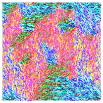
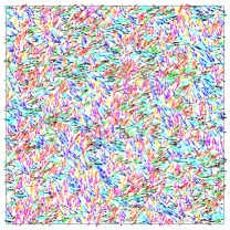
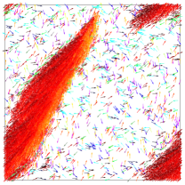
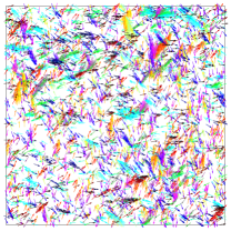
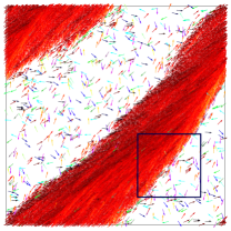
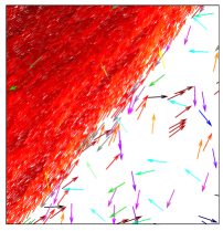
In this paper, we propose a model for self-propelled rods (SPRs) in two dimensions that interact with a physical interaction potential. We discretize each rod by a number of beads to calculate rod-rod interactions. In contrast to previous models with strict excluded-volume interactions Peruani et al. (2006); Yang et al. (2010); Wensink et al. (2012); McCandlish et al. (2012); Kraikivski et al. (2006); Peruani et al. (2006), our interaction potential allows rods to cross. Our simulations thus combine the computational efficiency of two-dimensional simulations with a possibility to mimic an escape to the third dimension when two rods collide. Simulation snapshots of the system which display disordered states, motile clusters, lanes, etc. are shown in Fig. 1, and movies can be found in the Supplemental Material Abk .
The paper is organized as follows. We introduce model, simulation methods, and numerical parameters in Sec. II. We calculate a phase diagram for passive (nonswimming) rods in Sec. III using Monte Carlo simulations, followed by a short discussion on the probability of crossing events in Sec. IV. We focus on cluster formation in Sec. V, introducing gas density and cluster break-up in Sec. V.1, cluster size analysis in Sec. V.2, and autocorrelation functions for rod orientations in Sec. V.3. We summarize our main results in Sec. VI.

II Model and Simulation Technique
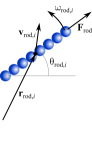
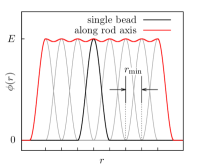
We simulate rods with and without an intrinsic propulsion force. Our systems consist of rods in a two-dimensional box of size with periodic boundary conditions; see Fig. 1. We use Brownian dynamics simulations for active systems and Monte Carlo simulations for passive systems. The rods are characterized by their center-of-mass positions , their orientation angles with respect to the axis, their center-of-mass velocities , and their angular velocities ; see Fig. 2. To calculate energy, force, and torque due to rod-rod interactions, we discretize each rod into beads, separated from each other by a distance of . Beads from different rods interact by a separation-shifted Lennard-Jones potential Fisher and Ruelle (1966),
| (1) |
where is the distance between two beads and gives the interaction energy. The potential is shifted by to avoid a discontinuity at . The parameter characterizes the capping of the potential. For , does not diverge at , hence allowing bead-bead overlap; for , becomes the truncated Lennard-Jones potential.
is the energy for two beads that completely overlap and is used as independent parameter in our simulations. Setting to any value will dictate . The constant is calculated by forcing to be zero at . Considering the weak repulsion between rods, we define as the effective radius for each bead, which results in the effective rod thickness and the rod aspect ratio . The number of beads used for discretization is chosen such that the rod has a relatively smooth potential profile, so that no interlocking occurs when rods slide along each other; see Fig. 2.
For the Brownian dynamics simulations, we decompose the rod velocity into parallel and perpendicular components with respect to its axis, . In each simulation step, the velocities are calculated using
| (2) | |||||
| (3) |
and
| (4) |
where and are unit vectors parallel and perpendicular to the rod axis, respectively. is the propulsion force for each rod. The friction coefficients are given by , , and , where is the rod length Yang et al. (2010). The random values , , and for the forces in parallel and perpendicular direction and for the torque are drawn from Gaussian distributions with variances , , and , respectively. We employ thermal noise, thus the variances are calculated using 111In biological and synthetic self-propelled systems, the noise arises from the environmental noise, for example, from density fluctuations of signaling molecules for chemotactic swimmers or from motor activity. In this case, the noise is not proportional to and also the coupling between translational and rotational noise may be different.. Finally, and are the force and torque from rod to rod , calculated using Eq. (1). Hydrodynamic interactions between the rods are largely screened because of the nearby wall and the high rod density Berke et al. (2008); Elgeti and Gompper (2009); Elgeti et al. (2010); Elgeti and Gompper (2013), and hence are neglected in our simulations.
We study systems with approximately rods at scaled number densities ranging from to , where the number density of rods is defined as . We measure lengths in units of rod length , energies in units of , and times in units of the orientational diffusion time for a single rod, . The system size is , the cutoff , the rod aspect ratio , the time interval , and unless mentioned otherwise, .
There are three different energy scales in our system; the thermal energy , the propulsion strength , and the energy barrier . Therefore, there are two dimensionless ratios that characterize the importance of the different contributions: the Péclet number, defined as 222The Péclet number can be alternatively defined as with the rotational diffusion constant . In such case, .
| (5) |
which is the ratio of propulsion strength to noise, and the penetrability coefficient, , defined as
| (6) |
which is the ratio of propulsion strength to energy barrier. is the diffusion coefficient parallel to the rod orientation.
We simulate rods with Péclet numbers in the range and penetrabilities in the range . We change by changing for fixed and , i. e., for fixed temperature. We change by changing both and .
III Isotropic-nematic transition for passive systems
Suspensions of passive rodlike particles in thermal equilibrium are isotropic for low densities and nematic for high densities Kayser and Raveché (1978). For and , the transition density has been predicted using Onsager’s theory for infinitely thin hard rods Kayser and Raveché (1978); Onsager (1944). For our systems with the capped potential given by Eq. (1), not only the aspect ratio of the rod but also the energy barrier affects the density for the isotropic-nematic transition. As becomes smaller, the tendency for rods to align becomes weaker because overlaps occur more frequently. For , the rods do not interact mutually and thus are in the isotropic phase for all densities.
We performed Brownian dynamics simulations for systems with at various densities. At low densities, , the systems are in an isotropic state as shown in Fig. 1(b). For high densities, , nematic states are found that are composed of large interlocked groups of rods with similar orientations; see Fig. 1(a). Because the simulation of passive rods with Brownian dynamics is computationally very expensive, we used Monte Carlo simulations to systematically study the state of the system for several values of and . We characterize the state using the nematic order parameter Kraikivski et al. (2006),
| (7) |
where the average is over cells of side length . and correspond to perfectly isotropic and nematic states, respectively.
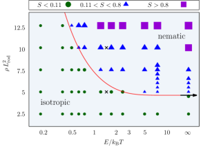
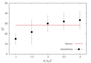
Figure 3 shows a phase diagram of the system with varying density and energy barrier. According to analytical theory Kayser and Raveché (1978), for the transition from the isotropic to the nematic state occurs at , as indicated by the black arrow in Fig. 3. This density corresponds to , which we thus define as threshold value to calculate the transition density for finite values of the energy barrier; see Appendix A. We have also calculated the density for the isotropic-nematic transition,
| (8) |
by generalizing Onsager’s approach for finite energy barriers, as described in Appendix A. We find very good agreement between the analytical theory shown by the red (gray) line in Fig. 3 and our Monte Carlo simulations. The phase diagram is also consistent with our Brownian dynamics simulations for and ; see snapshots in Figs. 1(a) and 1(b).
IV Crossing probability for rod-rod collisions
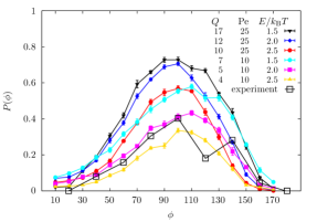
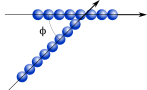
To find the probability of crossing events , we performed simulations for two rods that initially touch each other in a tip-center arrangement with crossing angle ; see Fig. 4. We measure for several penetrabilities and Péclet numbers using Brownian dynamics simulations. We count a crossing event when two rods intersect significantly, i. e., such that the intersection point is at least away from the ends of each rod. We thus do not count events when one rod only “touches” the other rod, which frequently happens due to the weak repulsion between the rods.
As shown in Fig. 4, is low near and and has a peak near . There is a small asymmetry in the peak with an enhancement for directions , which may be attributed to the increased relative velocity between two rods for and the fact that the rods are not perfectly smooth. Comparison between for different penetrabilities shows that an increased generally increases the probability for rod crossing. In addition, for small , noise also plays an important role to enhance rod crossing. For example, the curves for and in Fig. 4 have approximately the same height, and this could be explained by the fact that the effect of noise is higher for the case that has a smaller .
The results are qualitatively similar to the crossing probability measured in experiments with microtubules propelled on surfaces. In Fig. 3(d) in Ref. Sumino et al. (2012), the maximum crossing probability for two microtubules in a motility assay is and corresponds to and in our simulations. However, the same crossing probability may be achieved by reducing and increasing at the same time.
V Cluster formation for active systems
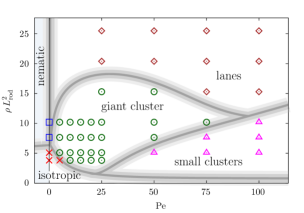
To characterize the collective behavior, we have performed simulations with large numbers of rods. After initiating the rods with random positions and orientations in the two-dimensional (2D) plane, the rods move by their propulsion force and are affected by interactions with other rods and thermal noise. Snapshots of the system are shown in Fig. 1. More snapshots and movies can be found in the Supplemental Material Abk . A phase diagram of self-propelled rods with varying density and Péclet number is shown in Fig. 5.
For , we find giant clusters that span the entire simulation box and form as a result of the alignment interaction due to the rod-rod repulsion, as explained qualitatively in Refs. Baskaran and Marchetti (2012); Ginelli et al. (2010); see Figs. 1(c) and 1(e). At the cluster perimeter, the clusters steadily lose rods due to the rotational diffusion and at the same time acquire new rods that collide and align. The clusters are polar and almost all rods within a giant cluster move in the same direction. However, we expect that the system is essentially in an isotropic phase, and that for a sufficiently large system size the clusters can randomly change direction. The polar order of our giant clusters which span the simulation box is due to symmetry-breaking collisions because of the roughness of the rods. In the early stage of the formation of giant clusters, some of the eventually polar clusters are composed of streams of rods that move in opposite directions.
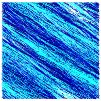
Upon further increase of the clusters start to break; see Fig. 1(d). Smaller clusters are observed until they become as small as about five rods per cluster for . For very high densities, , when the dense region spans the entire simulation box, we find a laning phase that is composed of streams of rods that move in opposite directions; see Fig. 1(g). The laning phase is nematic, similar to the nematic lanes that have been observed for the Vicsek model in simulations Ginelli et al. (2010) and analytical calculations Peshkov et al. (2012).
Our phase diagram in Fig. 5 may be compared with the phase diagram in Ref. Wensink et al. (2012) for self-propelled rods that interact segment-wise via a Yukawa potential. Since our model incorporates noise and has a capped repulsive interaction potential, we can only compare both models in the medium regime, where the noise does not dominate and where the rods are not completely penetrable . For aspect ratio used in our simulation, we see qualitatively similar behavior with increasing density, namely the transition from the isotropic phase to the swarming (clustering) phase and then to the laning phase.
A comparison of our phase diagram in Fig. 5 with that of Ref. Yang et al. (2010) shows that we do not observe jammed giant clusters as reported in Ref. Yang et al. (2010), because we employ a smoother potential profile along the rod; see Fig. 2.
V.1 Rod densities
(a)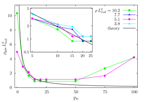
(b)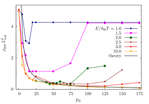
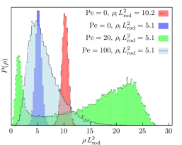
We measure densities of rods in cells of side length and construct a distribution of monomer densities for each system; see Fig. 6. For a homogeneous system of rods, the distribution has a single narrow peak at the average density of the system, . This can be seen for example in the histograms for that correspond to the systems where no cluster formation is observed; see Figs. 1(a) and 1(b). For systems with self-propelled rods, the density distribution can change from a binomial to a more complicated distribution that shows phase separation between dilute and dense regions of rods. For the distribution has a large peak at low density and a very broad peak at higher densities. The noise in the distribution is due to the poor statistics in the intermediate density regime. The system consists of a (high-density) cluster in a “gas” of rods; the density of this cluster-free region corresponds to the position of the first peak in the density distribution. In the following, we denote the density of this cluster-free region as .
In Fig. 7, is plotted as a function of for several values of and . We define as the position of the first local maximum in the density distribution, which is at least as high as of the absolute maximum. We find for small and an increase of with increasing for high . The gas density is to a large extent independent of the average rod density of the entire system;see Fig. 7(a). This behavior is analogous to the vapor density for liquid-gas phase coexistence in conventional liquids, where the density of the gas phase only depends on the temperature and is independent of the volume of the liquid phase.
The dependence of on and in the low range can be quantitatively explained by a rate equation Redner et al. (2013). In the stationary state, the rate of rods joining a cluster equals the rate of rods leaving a cluster. Assuming an isotropic distribution of rods in the gas, the number of rods joining the cluster from an infinitesimally small box of side length and is , where is the half angle of a cone inside which rods reach the wall in a given time , and is the distance to the cluster “wall.” Integrating over from to gives the attachment rate
| (9) |
where we have used the definition of Péclet number in Eq. (5).
The detachment rate is determined by the rotational diffusion of the rods; the typical time a rod needs to diffuse by an angle is
| (10) |
Assuming that a complete detachment from the cluster requires and that rods are placed regularly along the border of a cluster, the detachment rate is found to be
| (11) |
By equating and , we find as a function of ,
| (12) |
where we have used . Note that the gas density in Eq. (12) only depends on and and is independent of the average system density , which is consistent with the simulation results. This implies that the giant cluster grows until the density of the dilute region reaches .
Note that this estimate includes several approximations, in particular using free rotational diffusion for rods at the border of the cluster and assuming that complete detachment requires the rods to diffuse by . As shown in Fig. 7, the analytical estimate in Eq. (12) agrees well with the simulation results in the small- range without any adjustable parameters. Assuming a two-dimensional gas for the dilute rod phase, we can thus estimate an effective binding energy per rod for the rods inside the giant cluster,
| (13) | |||||
as explained in Appendix B. The effective binding strength increases logarithmically with the product of Péclet number and the rod aspect ratio. For aspect ratio and used in our simulations, we find effective binding energies of , which are comparable to binding energies for the gas-liquid critical point for colloidal systems Vliegenthart and Lekkerkerker (2000).
For , clusters break up when , which implies . We observe that in the regime of cluster break-up, individual rods and even small clusters can pass through each other. In our simulations is proportional to the propulsion force, and a high propulsion force thus facilitates crossing of rods. As a result, fewer rods aggregate in a large cluster and the rod density in the dilute region increases; see Fig. 7. Cluster break-up starts when the propulsion force, , is comparable with the maximum force for bead-bead interaction, . Equating to gives the critical value of the penetrability coefficient for cluster break-up,
| (14) |
where and is found by numerically solving for the potential in Eq. (1). In Fig. 8, is plotted for various energy barriers. Although the angular dependence for crossing of rods (Fig. 4) is neglected in the estimate in Eq. (14), we find reasonable agreement with the simulation results without any adjustable parameters. However, there is less agreement for small energy barriers, corresponding to small . The deviations may be accounted for by the noise that for small is comparable with the propulsion force (but that is not considered in the analytical estimate).
V.2 Cluster size distributions
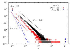
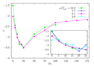
We define two rods to be in the same cluster if the nearest distance between them is less than and the difference in their orientation angles is less than . In Fig. 9, sample cluster size distributions are presented. For small cluster size , decreases with a power law, with ; for large , decreases exponentially Yang et al. (2010); Huepe and Aldana (2008). For systems with giant clusters, such as the system with , there is a gap in the distribution because they consist of one giant cluster and small clusters that mostly form near the boundary of the giant cluster. In such systems, the exponent is calculated only based on the distribution of small clusters.
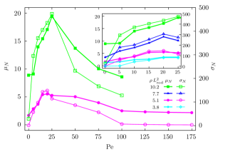
The power-law exponent for the cluster size distribution first decreases with increasing Péclet number, has a minimum for , and then increases for increasing the values of , see Fig. 10. We find the exponent to be in the range , which agrees with the range found in Ref. Yang et al. (2010) for rods with different aspect ratio and a different interaction potential than in our simulations. A recent experimental study found for clusters of M. xanthus bacteria Peruani et al. (2012). As shown in Fig. 11, the average size of the clusters, , increases with increasing Péclet number for and decreases if is further increased. The spread of the cluster size, , shows the same qualitative behavior but decays faster at high values, which shows that the system becomes more homogeneous.
V.3 Polar autocorrelation functions
(a)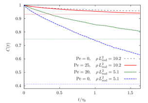
(b)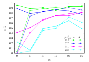
(c)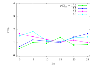
The clustering dynamics in the systems can be characterized by autocorrelation functions for the rod orientation
| (15) |
for lag time , where is the orientation vector of rod at time , and the average is over all rods and over all times . Figure 12(a) shows for systems shown in Fig. 1. The autocorrelation function can be fit using a shifted exponential function
| (16) |
where is the autocorrelation time and is an autocorrelation base value. A finite value of is the ratio of rods that do not lose their orientation for the time scale of the measurement. Rods that are inside clusters are less likely to lose their orientation, which corresponds to a high value of , while free rods in the gas change orientation more frequently because of rotational diffusion.
In Fig. 12(b), we compare to the averaged fraction of rods that are part of the largest cluster in the system for several densities and Péclet numbers. In general, we find good agreement between and 333The values of and do not agree for , where rods are either freely moving due to noise (isotropic regime) or stuck in small nonmotile clusters (nematic regime). In the former case, there is hardly any orientation preservation () and there is no large cluster (). In the latter case, rods hardly change their orientation () but are distributed over small clusters ().. The autocorrelation time , shown in Fig. 12(c), does not change substantially for different values of and . The correlation time obtained from the fit with Eq. (16) is very similar to the autocorrelation time for a single rod, which shows that the rotational diffusion is only weakly affected by occasional collisions of the rods. Therefore, the giant cluster moves persistently within simulation time.
VI Summary and Conclusions
We have studied collective behavior for self-propelled rigid rods in two dimensions constructed by single beads that interact with a separation-shifted Lennard Jones potential. The finite potential strength mimics the ability of microswimmers close to a wall and of filaments in motility assays to temporarily escape to the third dimension and cross each other. For a high potential barrier, we recover the limit of impenetrable rods studied, for example, in Refs. Yang et al. (2010); Wensink et al. (2012). For most simulations, we have used an interaction energy that for complete overlap of two beads is of the order of the thermal energy; crossing of rods therefore occurs with a high probability; see Fig. 4. However, the interaction energy is much larger than the bead-bead interaction energy if rods cross at a small angle or if a single rod approaches a cluster. For our system with beads per rod, the energy for complete overlap is and thus the probability for such events is very low.
We have calculated a phase diagram for rod density and energy barrier to characterize the isotropic-nematic transition for passive rods. The isotropic-nematic transition is shifted to higher densities for reduced overlap energy, because of the reduced rod-rod interaction. We find significant deviations from the transition density calculated for hard rods Onsager (1944); Kayser and Raveché (1978) if the bead-bead interaction energy is below . For , the isotropic-nematic transition occurs for , where is the transition density for hard rods Kayser and Raveché (1978). Our results using a modified Onsager theory show excellent agreement with our Monte Carlo simulations.
Using Brownian dynamics simulations, we have determined the crossing probability for two colliding rods as function of their relative angles for several values of penetrability coefficient and Péclet number. The crossing probability is highest for almost perpendicular collisions, which is qualitatively similar to the crossing probability measured in experiments with microtubules propelled on surfaces. In Ref. Sumino et al. (2012), the maximum crossing probability for two microtubules in a motility assay is and corresponds to and in our simulations 444The same crossing probability may be achieved by increasing and at the same time..
Self-propelled rods align due to their soft repulsive interaction Baskaran and Marchetti (2012). For high rod densities, we find a laning phase. For intermediate rod densities and Péclet numbers, we observe the formation of giant clusters that span the entire simulation box, which we denote as “clustering window.” Clusters break if the propulsion force is strong enough to overcome the repulsive force due to rod-rod interaction. We find a critical value for cluster break-up. We characterize our systems by cluster size distributions that can be fit by power-laws with , which is consistent with previous experimental and simulation results Yang et al. (2010); Peruani et al. (2012). By analyzing the autocorrelation function for rod orientation, we can separate the contributions from rods in a cluster from the contributions from free rods. We find that the free rods show almost the same orientational correlation as single rods.
We can analytically estimate the density of free rods in systems with giant clusters, which we denote as “gas density,” . The gas density is independent of the average rod density in the system, which is analogous to the molecule density in the gas phase for liquid-gas coexistence that does not depend on the volume of the liquid phase but only on temperature. Using , we calculate effective binding energies for rods in the cluster. For aspect ratio used in our simulations and , we find effective binding energies of about , which is comparable to binding energies for the gas-liquid critical point for colloidal systems Vliegenthart and Lekkerkerker (2000).
Phase separation into high-density and low-density regions is an intrinsic property of self-propelled particle systems and has also been observed for nonaligning spherical particles Tailleur and Cates (2008); Fily and Marchetti (2012); Redner et al. (2013); Wysocki et al. . As for the rods, the gas density of the spheres is inversely proportional to the propulsion velocity Redner et al. (2013). However, the nature of cluster formation is different in the two models: While we observe motile clusters as a result of particle alignment, systems with nonaligning spheres exhibit jammed nonmotile clusters as a result of steric trapping. Moreover, the internal structure of clusters is nematic in our model, contrary to the isotropic structure for nonaligning spheres. Of course, also laning phases are only possible for anisotropic particles.
We have introduced and characterized a model of self-propelled rods that interact with a physical interaction that allows for crossing events. The model can now be used to interpret experiments for almost two-dimensional systems with good computational efficiency and allows predictions beyond those based on models using point particles with phenomenological alignment rules.
Acknowledgements.
We thank Adam Wysocki and Jens Elgeti for stimulating discussions. M.A. and K.M. acknowledge support by the International Helmholtz Research School of Biophysics and Soft Matter (IHRS BioSoft). CPU time allowance from the Jülich Supercomputing Centre (JSC) is gratefully acknowledged.Appendix A Phase transition of passive rods
The nematic order parameter is plotted in Fig. 13 for various cuts through the phase diagram in Fig. 3. It has been suggested that the isotropic-nematic transition of rods is continuous in two dimensions Kayser and Raveché (1978). We have chosen a threshold value for the isotropic-nematic phase transition, , such that for an infinite interaction energy the value predicted by the Onsager theory is recovered. Our threshold value is similar to the threshold value that has been chosen in Ref. Kraikivski et al. (2006).
(a)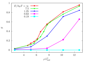
(b)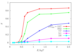
For finite energy barrier , we generalize the approach presented in Ref. Kayser and Raveché (1978) based on bifurcation theory to obtain the critical density for the isotropic-nematic transition. The distribution function for the rod orientation is given by , which satisfies
| (17) |
where the constant is determined by the normalization of ,
| (18) |
We define as
| (19) |
such that corresponds to an isotropic distribution. Using Eqs. (17)–(19), we can write
| (20) |
We assume that the interaction energy of two rods is either or , depending on whether they cross each other. This approximation is justified if the rods are very thin and the complete overlap of two rods—which is energetically very unfavorable—is excluded. In the regime where , the parameter and the kernel are given by
| (21) | |||||
Substituting Eqs. (21) and (A) in Eq. (20) gives
| (23) |
where the operator is defined as
For to have bifurcation point in ,
| (25) |
has to have an eigenfunction with two maxima at and no further maxima. The corresponding eigenvalue determines the density at which bifurcation occurs. The desired eigenfunction is with the eigenvalue ; thus the bifurcation density that corresponds to the isotropic-nematic transition is
| (26) |
Appendix B Effective binding energy for rod adsorption to the cluster
The independence of gas density from the average density of the system is analogous to a vapor density for rods. Here we follow this analogy to obtain an effective binding energy gain for rods that are part of the cluster.
We use an ideal-gas model in two dimensions to represent the rods in the gas phase. The activity and the anisotropy of the rods are intentionally not taken into account explicitly and enter via the effective binding energy. The free energy for the rods in the gas is thus
where is the number of rods in the gas, is the area of each rod, and is the area accessible for the rods in the gas.
In the cluster, each rod gains a binding energy ,
| (28) |
where here is the number of rods in the cluster. In equilibrium, the chemical potential in the gas and in the cluster should be equal. This gives Eq. (13).
References
- Vicsek and Zafeiris (2012) T. Vicsek and A. Zafeiris, Phys. Rep. 517, 71 (2012).
- Riedel et al. (2005) I. H. Riedel, K. Kruse, and J. Howard, Sci. Signal. 309, 300 (2005).
- Yang et al. (2008) Y. Yang, J. Elgeti, and G. Gompper, Phys. Rev. E 78, 061903 (2008).
- Ben-Jacob et al. (2000) E. Ben-Jacob, I. Cohen, and H. Levine, Adv. Phys. 49, 395 (2000).
- Sokolov et al. (2007) A. Sokolov, I. S. Aranson, J. O. Kessler, and R. E. Goldstein, Phys. Rev. Lett. 98, 158102 (2007).
- Peruani et al. (2012) F. Peruani, J. Starruß, V. Jakovljevic, L. Søgaard-Andersen, A. Deutsch, and M. Bär, Phys. Rev. Lett. 108, 098102 (2012).
- Gachelin et al. (2013) J. Gachelin, G. Miño, H. Berthet, A. Lindner, A. Rousselet, and E. Clément, Phys. Rev. Lett. 110, 268103 (2013).
- Paxton et al. (2004) W. F. Paxton, K. C. Kistler, C. C. Olmeda, A. Sen, S. K. St. Angelo, Y. Cao, T. E. Mallouk, P. E. Lammert, and V. H. Crespi, J. Am. Chem. Soc. 126, 13424 (2004).
- Volpe et al. (2011) G. Volpe, I. Buttinoni, D. Vogt, H.-J. Kummerer, and C. Bechinger, Soft Matter 7, 8810 (2011).
- Mei et al. (2011) Y. Mei, A. A. Solovev, S. Sanchez, and O. G. Schmidt, Chem. Soc. Rev. 40, 2109 (2011).
- Ebbens et al. (2012) S. Ebbens, M.-H. Tu, J. R. Howse, and R. Golestanian, Phys. Rev. E 85, 020401 (2012).
- Yang and Ripoll (2011) M. Yang and M. Ripoll, Phys. Rev. E 84, 061401 (2011).
- Harada et al. (1987) Y. Harada, A. Noguchi, A. Kishino, and T. Yanagida, Nature (London) 326, 805 (1987).
- Schaller et al. (2010) V. Schaller, C. Weber, C. Semmrich, E. Frey, and A. R. Bausch, Nature (London) 467, 73 (2010).
- Sumino et al. (2012) Y. Sumino, K. H. Nagai, Y. Shitaka, D. Tanaka, K. Yoshikawa, H. Chaté, and K. Oiwa, Nature (London) 483, 448 (2012).
- Lauga et al. (2006) E. Lauga, W. R. DiLuzio, G. M. Whitesides, and H. A. Stone, Biophys. J. 90, 400 (2006).
- Berke et al. (2008) A. P. Berke, L. Turner, H. C. Berg, and E. Lauga, Phys. Rev. Lett. 101, 038102 (2008).
- Elgeti and Gompper (2009) J. Elgeti and G. Gompper, EPL 85, 38002 (2009).
- Elgeti et al. (2010) J. Elgeti, U. B. Kaupp, and G. Gompper, Biophys. J. 99, 1018 (2010).
- Elgeti and Gompper (2013) J. Elgeti and G. Gompper, EPL 101, 48003 (2013).
- Vicsek et al. (1995) T. Vicsek, A. Czirók, E. Ben-Jacob, I. Cohen, and O. Shochet, Phys. Rev. Lett. 75, 1226 (1995).
- Toner and Tu (1995) J. Toner and Y. Tu, Phys. Rev. Lett. 75, 4326 (1995).
- Simha and Ramaswamy (2002) R. A. Simha and S. Ramaswamy, Phys. Rev. Lett. 89, 058101 (2002).
- Ramaswamy et al. (2003) S. Ramaswamy, R. A. Simha, and J. Toner, Europhys. Lett. 62, 196 (2003).
- Toner et al. (2005) J. Toner, Y. Tu, and S. Ramaswamy, Ann. Phys. 318, 170 (2005).
- Peruani et al. (2008) F. Peruani, A. Deutsch, and M. Bär, Eur. Phys. J. Special Topics 157, 111 (2008).
- Bertin et al. (2009) E. Bertin, M. Droz, and G. Grégoire, J. Phys. A: Math. Theor. 42, 445001 (2009).
- Golestanian (2009) R. Golestanian, Phys. Rev. Lett. 102, 188305 (2009).
- Redner et al. (2013) G. S. Redner, M. F. Hagan, and A. Baskaran, Phys. Rev. Lett. 110, 055701 (2013).
- Szabó et al. (2006) B. Szabó, G. J. Szöllösi, B. Gönci, Z. Jurányi, D. Selmeczi, and T. Vicsek, Phys. Rev. E 74, 061908 (2006).
- Grégoire and Chaté (2004) G. Grégoire and H. Chaté, Phys. Rev. Lett. 92, 025702 (2004).
- Huepe and Aldana (2004) C. Huepe and M. Aldana, Phys. Rev. Lett. 92, 168701 (2004).
- D’Orsogna et al. (2006) M. R. D’Orsogna, Y. L. Chuang, A. L. Bertozzi, and L. S. Chayes, Phys. Rev. Lett. 96, 104302 (2006).
- Aldana et al. (2007) M. Aldana, V. Dossetti, C. Huepe, V. M. Kenkre, and H. Larralde, Phys. Rev. Lett. 98, 095702 (2007).
- Chaté et al. (2008) H. Chaté, F. Ginelli, G. Grégoire, and F. Raynaud, Phys. Rev. E 77, 046113 (2008).
- Ginelli et al. (2010) F. Ginelli, F. Peruani, M. Bär, and H. Chaté, Phys. Rev. Lett. 104, 184502 (2010).
- Baskaran and Marchetti (2008a) A. Baskaran and M. C. Marchetti, Phys. Rev. E 77, 011920 (2008a).
- McCandlish et al. (2012) S. R. McCandlish, A. Baskaran, and M. F. Hagan, Soft Matter 8, 2527 (2012).
- Baskaran and Marchetti (2008b) A. Baskaran and M. C. Marchetti, Phys. Rev. Lett. 101, 268101 (2008b).
- Yang et al. (2010) Y. Yang, V. Marceau, and G. Gompper, Phys. Rev. E 82, 031904 (2010).
- Wensink et al. (2012) H. H. Wensink, J. Dunkel, S. Heidenreich, K. Drescher, R. E. Goldstein, H. Löwen, and J. M. Yeomans, Proc. Natl. Acad. Sci. U.S.A. 109, 14308 (2012).
- Kraikivski et al. (2006) P. Kraikivski, R. Lipowsky, and J. Kierfeld, Phys. Rev. Lett. 96, 258103 (2006).
- Costanzo et al. (2012) A. Costanzo, R. Di Leonardo, G. Ruocco, and L. Angelani, J. Phys. Condens. Matter 24, 065101 (2012).
- Peruani et al. (2006) F. Peruani, A. Deutsch, and M. Bär, Phys. Rev. E 74, 030904 (2006).
- Peruani et al. (2010) F. Peruani, L. Schimansky-Geier, and M. Bär, Eur. Phys. J. Special Topics 191, 173 (2010).
- Huepe and Aldana (2008) C. Huepe and M. Aldana, Phys. A (Amsterdam, Neth.) 387, 2809 (2008).
- Ruhnow et al. (2011) F. Ruhnow, D. Zwicker, and S. Diez, Biophys. J. 100, 2820 (2011).
- (48) See Supplemental Material at [URL] for movies of self-propelled rod systems .
- Fisher and Ruelle (1966) M. E. Fisher and D. Ruelle, J. Math. Phys. 7, 260 (1966).
- Note (1) In biological and synthetic self-propelled systems, the noise arises from the environmental noise, for example, from density fluctuations of signaling molecules for chemotactic swimmers or from motor activity. In this case, the noise is not proportional to and also the coupling between translational and rotational noise may be different.
- Note (2) The Péclet number can be alternatively defined as with the rotational diffusion constant . In such case, .
- Kayser and Raveché (1978) R. F. Kayser and H. J. Raveché, Phys. Rev. A 17, 2067 (1978).
- Onsager (1944) L. Onsager, Phys. Rev. 65, 117 (1944).
- Baskaran and Marchetti (2012) A. Baskaran and M. C. Marchetti, Eur. Phys. J. E 35, 1 (2012).
- Peshkov et al. (2012) A. Peshkov, I. S. Aranson, E. Bertin, H. Chaté, and F. Ginelli, Phys. Rev. Lett. 109, 268701 (2012).
- Vliegenthart and Lekkerkerker (2000) G. Vliegenthart and H. N. Lekkerkerker, J. Chem. Phys. 112, 5364 (2000).
- Note (3) The values of and do not agree for , where rods are either freely moving due to noise (isotropic regime) or stuck in small nonmotile clusters (nematic regime). In the former case, there is hardly any orientation preservation () and there is no large cluster (). In the latter case, rods hardly change their orientation () but are distributed over small clusters ().
- Note (4) The same crossing probability may be achieved by increasing and at the same time.
- Tailleur and Cates (2008) J. Tailleur and M. E. Cates, Phys. Rev. Lett. 100, 218103 (2008).
- Fily and Marchetti (2012) Y. Fily and M. C. Marchetti, Phys. Rev. Lett. 108, 235702 (2012).
- (61) A. Wysocki, R. G. Winkler, and G. Gompper, arXiv:1308.6423 [cond-mat.soft] .