Efficient additive Schwarz preconditioning for hypersingular integral equations
on locally refined triangulations

Abstract.

For non-preconditioned Galerkin systems, the condition number grows with the number of elements as well as the quotient of the maximal and the minimal mesh-size. Therefore, reliable and effective numerical computations, in particular on adaptively refined meshes, require the development of appropriate preconditioners. We analyze and numerically compare multilevel additive Schwarz preconditioners for hypersingular integral equations, where 2D and 3D as well as closed boundaries and open screens are covered. The focus is on a new local multilevel preconditioner which is optimal in the sense that the condition number of the corresponding preconditioned system is independent of the number of elements, the local mesh-size, and the number of refinement levels.

1. Introduction

Let $\Omega\subset{\mathbb{R}}^{d}$ be a bounded polygonal resp. polyhedral Lipschitz domain in ${\mathbb{R}}^{d}$, $d=2,3$, with connected boundary $\Gamma=\partial\Omega$. For a given right-hand side $f$, we consider the hypersingular integral equation

(1) $$\mathcal{W}u(x):=-\partial_{\boldsymbol{n}_{x}}\int_{\Gamma}\partial_{\boldsymbol{n}_{y}}G(x-y)u(y)\,ds_{y}=f(x)\quad\text{for }x\in\Gamma.$$

Here, $\partial_{\boldsymbol{n}_{x}}$ is the normal derivative with respect to $x\in\Gamma$, and $G(z)$ denotes the fundamental solution of the Laplacian

(2) $$G(z)=\begin{cases}-\frac{1}{2\pi}\log|z|&\text{for }d=2,\\ +\frac{1}{4\pi}\frac{1}{|z|}&\text{for }d=3.\end{cases}$$

The exact solution $u$ of (1) cannot be computed analytically in general. For a given triangulation ${\mathcal{T}}_{\ell}$ of $\Gamma$, one can e.g. use the Galerkin boundary element method (BEM) to compute an approximation $u_{\ell}$ of $u$ instead. If a certain accuracy of the approximation $u_{\ell}\approx u$ is required, adaptive mesh-refining algorithms of the type

$$\boxed{\texttt{ SOLVE }}\quad\longrightarrow\quad\boxed{\texttt{ ESTIMATE }}\quad\longrightarrow\quad\boxed{\texttt{ MARK }}\quad\longrightarrow\quad\boxed{\texttt{ REFINE }}$$

are used, where, starting with a given initial triangulation ${\mathcal{T}}_{0}$, a sequence of locally refined triangulations ${\mathcal{T}}_{\ell}$ and corresponding Galerkin solutions $u_{\ell}$ are computed. The lowest-order BEM for (1) uses ${\mathcal{T}}_{\ell}$-piecewise affine and globally continuous functions $u_{\ell}\in\SS^{1}({\mathcal{T}}_{\ell})$ to approximate $u$, and the adaptive mesh-refinement leads to a nested sequence of spaces $\SS^{1}({\mathcal{T}}_{\ell})\subset\SS^{1}({\mathcal{T}}_{\ell+1})$ for all $\ell\geq 0$.

In recent years, the convergence of adaptive BEM even with quasi-optimal algebraic rates has been proved [FKMP13, Tso13, FFK⁺13a, FFK⁺13b]. Throughout, it is however assumed that the Galerkin solution $u_{\ell}$ is computed exactly, i.e. the resulting linear system $\mathbf{A}^{\ell}{\mathbf{x}}^{\ell}={\bf b}^{\ell}$ is solved exactly. As is well known, the accuracy of direct solvers as well as the effectivity of iterative solvers is usually spoiled by the conditioning of the matrix $\mathbf{A}^{\ell}$. For uniform triangulations ${\mathcal{T}}_{\ell}$ with number of elements $N_{\ell}=\#{\mathcal{T}}_{\ell}$, it holds ${\rm cond}_{2}(\mathbf{A}^{\ell})\lesssim N_{\ell}^{1/(d-1)}$ for the $\ell_{2}$-condition number. For adaptively refined triangulations ${\mathcal{T}}_{\ell}$ with maximal element diameter $h_{{\rm max},\ell}$ and minimal element diameter $h_{{\rm min},\ell}$ the situation is even worse [AMT99], namely ${\rm cond}_{2}(\mathbf{A}^{\ell})\lesssim N_{\ell}(1+|\log(N_{\ell}h_{{\rm min},\ell})|)$ for $d=2$ resp. ${\rm cond}_{2}(\mathbf{A}^{\ell})\lesssim N_{\ell}^{1/2}(h_{{\rm max},\ell}/h_{{\rm min},\ell})^{2}$ for $d=3$.

Therefore, reliable and effective numerical computations require the development of efficient preconditioners. Prior work includes diagonal scaling of the BEM matrices which reduces the condition number for adaptive triangulations down to that of a uniform triangulation with the same number of elements [AMT99, GM06]. Other preconditioners for the Galerkin BEM of hypersingular integral equations are proposed in [TSM97, SW98, TSZ98, Cao02] and the references therein, where mainly quasi-uniform triangulations are thoroughly analyzed.

Our work focuses on additive Schwarz preconditioners for the Galerkin BEM of (1) with lowest-order polynomials $u_{\ell}\in\SS^{1}({\mathcal{T}}_{\ell})$. For uniform triangulations, it is shown in [TS96] that this approach leads to bounded condition numbers for the preconditioned system, i.e. ${\rm cond}((\mathbf{B}^{\ell})^{-1}\mathbf{A}^{\ell})\leq C<\infty$ with some $\ell$-independent constant $C>0$. The same is proved for partially adapted triangulations in [AM03], where it is assumed that ${\mathcal{T}}_{\ell}\cap{\mathcal{T}}_{\ell+1}\subset{\mathcal{T}}_{\ell+k}$ for all $\ell,k\in{\mathbb{N}}_{0}$, i.e. as soon as an element $T\in{\mathcal{T}}_{\ell}$ is not refined, it remains non-refined in all succeeding triangulations. In our contribution, we remove such an assumption which is infeasible in practice, and only rely on nestedness $\SS^{1}({\mathcal{T}}_{\ell})\subset\SS^{1}({\mathcal{T}}_{\ell+1})$ of the discrete ansatz spaces. The main idea is to use only new nodes in ${\mathcal{T}}_{\ell+1}\backslash{\mathcal{T}}_{\ell}$ plus their neighbouring nodes for preconditioning. In the frame of 2D FEM problems, such an idea has already been considered in the works [Mit92, WC06, XCH10]. For a V-cycle multigrid method, stability for the subspace decomposition in $H^{1}$ has been proved in [WC06] by means of a variant of the Scott-Zhang projection [SZ90]. In our work, we extend these results to the fractional-order Sobolev space $H^{1/2}$.

First, we give the analysis for the case $\Gamma=\partial\Omega$ and a stabilized Galerkin formulation which factors the constant functions out. We stress that the results of this work also apply to screens $\Gamma\subsetneqq\partial\Omega$, and the corresponding analysis is obtained by simply omitting all stabilization related terms. We also refer to the short Section 6 for further remarks.

While all constants and their dependencies are explicitly given in all statements, in proofs we use the symbol $\lesssim$ to abbreviate $\leq$ up to some multiplicative constant which is clear from the context. Moreover, we use $\simeq$ to abbreviate that both estimates $\lesssim$ and $\gtrsim$ holds.

The remainder of this work is organized as follows: Section 2 contains the analytical main result of this work. We first recall the necessary notation to define the new local multilevel preconditioner and then formulate the main result (Theorem 1). Furthermore, we introduce a global multilevel preconditioner and give a similar but weaker result (Theorem 2). For the ease of presentation, we first focus on closed boundaries. Section 3 formulates other preconditioners. Numerical experiments on closed boundaries and slits in 2D compare the condition numbers of the corresponding preconditioners as well as those with no preconditioning. In both, theory and practice, the new local multilevel preconditioner proves to be optimal in the sense that the condition number remains uniformly bounded which is not the case for the other strategies considered. In Section 4 we give a proof of Theorem 1 and in Section 5 we give a proof of Theorem 2. The final Section 6 comments on extension of the analysis to open screens in 2D and 3D. We show that the main result for the local and global multilevel preconditioner also hold for problems on open screens $\Gamma\subsetneqq\partial\Omega$ in 2D and 3D.

2. Main result

2.1. Continuous setting

Let $\Gamma:=\partial\Omega$. By $H^{s}(\Gamma)$, we denote the usual Sobolev spaces which are, e.g., given by real interpolation $H^{s}(\Gamma)=[L^{2}(\Gamma);H^{1}(\Gamma)]_{s}$, for $0<s<1$, and we let $H^{0}(\Gamma):=L^{2}(\Gamma)$. The space $H^{-s}(\Gamma):=H^{s}(\Gamma)^{*}$ is the dual space of $H^{s}(\Gamma)$, where duality is understood with respect to the extended $L^{2}(\Gamma)$-scalar product $\langle\cdot\,,\,\cdot\rangle_{\Gamma}$.

It is known that $\mathcal{W}$ induces a linear and bounded operator $\mathcal{W}:H^{s}(\Gamma)\to H^{s-1}(\Gamma)$, for all $0\leq s\leq 1$ which is symmetric and positive semidefinite on $H^{1/2}(\Gamma)$. Moreover, it holds $\langle\mathcal{W}v\,,\,1\rangle_{\Gamma}=0$. Let $H_{0}^{\pm 1/2}(\Gamma):=\big{\{}v\in H^{\pm 1/2}(\Gamma)\,:\,\langle v\,,\,1\rangle_{\Gamma}=0\big{\}}$. We thus suppose that the right-hand side $f$ in (1) satisfies $f\in H^{-1/2}_{0}(\Gamma)$.

As $\Gamma$ is connected, the kernel of $\mathcal{W}$ are precisely the constant functions, and thus $\mathcal{W}:H_{0}^{1/2}(\Gamma)\to H_{0}^{-1/2}(\Gamma)$ is linear, continuous, symmetric, and elliptic. By virtue of the Rellich compactness theorem, the definition

(3) $$\langle\langle v\,,\,w\rangle\rangle:=\langle\mathcal{W}v\,,\,w\rangle_{\Gamma}+\langle v\,,\,1\rangle_{\Gamma}\langle w\,,\,1\rangle_{\Gamma}$$

provides a scalar product on $H^{1/2}(\Gamma)$, and the induced norm $|||v|||^{2}:=\langle\langle v\,,\,v\rangle\rangle$ is equivalent to the usual $H^{1/2}(\Gamma)$-norm. In particular, the hypersingular integral equation (1) is equivalently recast in the variational formulation

(4) $$\langle\langle u\,,\,v\rangle\rangle=\langle f\,,\,v\rangle_{\Gamma}\quad\text{for all }v\in H^{1/2}(\Gamma).$$

According to the Lax-Milgram lemma, this formulation allows for a unique solution $u\in H^{1/2}(\Gamma)$. Due to $f\in H^{-1/2}_{0}(\Gamma)$, it follows $u\in H^{1/2}_{0}(\Gamma)$.

2.2. Triangulation and general notation

Let ${\mathcal{T}}_{\ell}$ denote a regular triangulation of $\Gamma$ into compact affine line segments ($d=2$) resp. compact plane surface triangles ($d=3$). We define the local mesh-width function $h_{\ell}\in L^{\infty}(\Gamma)$ by

(5) $$h_{\ell}|_{T}:=h_{\ell}(T):={\rm diam}(T)\quad\text{for all }T\in{\mathcal{T}}_{\ell}.$$

We suppose that ${\mathcal{T}}_{\ell}$ is $\gamma$-shape regular in the sense that

(6) $$h_{\ell}(T)\leq\gamma\,h_{\ell}(T^{\prime})\quad\text{and}\quad h_{\ell}(T)\leq\gamma\,|T|^{1/(d-1)}$$

for all $T,T^{\prime}\in{\mathcal{T}}_{\ell}$ with $T\cap T^{\prime}\neq\emptyset$. Here and throughout, $|T|$ denotes the $(d-1)$-dimensional surface measure of $T\in{\mathcal{T}}_{\ell}$ and hence $|T|={\rm diam}(T)$ for $d=2$. We note that for either dimension $d=2,3$, one of the conditions in (6) is automatically satisfied.

We consider lowest-order conforming boundary elements, where

(7) $${\mathcal{X}}^{\ell}:=\SS^{1}({\mathcal{T}}_{\ell}):=\big{\{}v\in C(\Gamma)\,:\,v|_{T}\text{ is affine for all }T\in{\mathcal{T}}_{\ell}\big{\}}.$$

Let ${\mathcal{N}}_{\ell}$ denote the set of nodes of the mesh ${\mathcal{T}}_{\ell}$. The natural basis of ${\mathcal{X}}^{\ell}$ is given by the hat-functions. For each node $z\in{\mathcal{N}}_{\ell}$, let $\eta_{z}^{\ell}\in\SS^{1}({\mathcal{T}}_{\ell})$ be the hat-function characterized by

(8) $$\eta_{z}^{\ell}(z)=1\quad\text{and}\quad\eta_{z}^{\ell}(z^{\prime})=0\quad\text{for all }z^{\prime}\in{\mathcal{N}}_{\ell}\backslash\{z\}.$$

For any subset $\tau\subseteq\Gamma$, we define the patch $\omega_{\ell}^{k}(\tau)\subseteq\Gamma$ inductively by

(9) $$\omega_{\ell}^{1}(\tau):=\omega_{\ell}(\tau):=\bigcup\big{\{}T\in{\mathcal{T}}_{\ell}\,:\,T\cap\tau\neq\emptyset\big{\}},\quad\omega_{\ell}^{k+1}(\tau):=\omega_{\ell}^{k}(\omega_{\ell}(\tau))\quad\text{for }k\in{\mathbb{N}}.$$

For any node $z\in{\mathcal{T}}_{\ell}$, we abbreviate $\omega_{\ell}^{k}(z):=\omega_{\ell}^{k}(\{z\})$ and note that $\omega_{\ell}(z)={\rm supp}(\eta_{z}^{\ell})$.

As in [WC06], we further define for every node $z\in{\mathcal{N}}_{\ell}$ the mesh-width $h_{\ell}(z)$ as the shortest edge $E$ of ${\mathcal{T}}_{\ell}$ with $z\in E$. It holds

(10) $$h_{\ell}(z)\leq h_{\ell}(T)\lesssim h_{\ell}(z)\quad\text{for all }z\in{\mathcal{N}}_{\ell}\text{ and }T\in{\mathcal{T}}_{\ell}\text{ with }z\in T,$$

where the hidden constant depends only on the $\gamma$-shape regularity of ${\mathcal{T}}_{\ell}$. The hat-functions satisfy

(11) $$\begin{split}0\leq\eta_{z}^{\ell}\leq 1,\quad\|\nabla\eta_{z}^{\ell}\|_{L^{\infty}(\Gamma)}\lesssim h_{\ell}^{-1}(z),\quad\text{and}\quad\sum_{z\in{\mathcal{N}}_{\ell}}\eta_{z}^{\ell}=1,\end{split}$$

where the hidden constant depends only on the $\gamma$-shape regularity of ${\mathcal{T}}_{\ell}$.

2.3. Galerkin discretization

The Galerkin solution $u_{\ell}\in{\mathcal{X}}^{\ell}$ to the solution $u$ of (4) solves

(12) $$\langle\langle u_{\ell}\,,\,v_{\ell}\rangle\rangle=\langle f\,,\,v_{\ell}\rangle_{\Gamma}\quad\text{for all }v_{\ell}\in{\mathcal{X}}^{\ell}.$$

Fixing a numbering of the nodes ${\mathcal{N}}_{\ell}=\{z_{1},\dots,z_{N}\}$, the discrete solution $u_{\ell}$ from (12) is obtained by solving a linear system of equations $\mathbf{A}^{\ell}{\mathbf{x}}^{\ell}={\bf b}^{\ell}$ in ${\mathbb{R}}^{N}$, where

(13) $$\mathbf{A}^{\ell}_{jk}=\langle\langle\eta_{z_{k}}^{\ell}\,,\,\eta_{z_{j}}^{\ell}\rangle\rangle,\quad{\bf b}^{\ell}_{j}=\langle f\,,\,\eta_{z_{j}}^{\ell}\rangle_{\Gamma},\quad\text{and}\quad u_{\ell}=\sum_{k=1}^{N}{\mathbf{x}}^{\ell}_{k}\eta_{z_{k}}^{\ell}.$$

\psfrag{T0}{}\psfrag{T1}{}\psfrag{T2}{}\psfrag{T3}{}\psfrag{T4}{}\psfrag{T12}{}\psfrag{T34}{}\includegraphics[width=99.58464pt]{nvb/bisec1_00}

\psfrag{T0}{}\psfrag{T1}{}\psfrag{T2}{}\psfrag{T3}{}\psfrag{T4}{}\psfrag{T12}{}\psfrag{T34}{}\includegraphics[width=99.58464pt]{nvb/bisec2left_00}

\psfrag{T0}{}\psfrag{T1}{}\psfrag{T2}{}\psfrag{T3}{}\psfrag{T4}{}\psfrag{T12}{}\psfrag{T34}{}\includegraphics[width=99.58464pt]{nvb/bisec2right_00}

\psfrag{T0}{}\psfrag{T1}{}\psfrag{T2}{}\psfrag{T3}{}\psfrag{T4}{}\psfrag{T12}{}\psfrag{T34}{}\includegraphics[width=99.58464pt]{nvb/bisec3_00}

\psfrag{T0}{}\psfrag{T1}{}\psfrag{T2}{}\psfrag{T3}{}\psfrag{T4}{}\psfrag{T12}{}\psfrag{T34}{}\includegraphics[width=99.58464pt]{nvb/bisec1_01}

\psfrag{T0}{}\psfrag{T1}{}\psfrag{T2}{}\psfrag{T3}{}\psfrag{T4}{}\psfrag{T12}{}\psfrag{T34}{}\includegraphics[width=99.58464pt]{nvb/bisec2left_01}

\psfrag{T0}{}\psfrag{T1}{}\psfrag{T2}{}\psfrag{T3}{}\psfrag{T4}{}\psfrag{T12}{}\psfrag{T34}{}\includegraphics[width=99.58464pt]{nvb/bisec2right_01}

\psfrag{T0}{}\psfrag{T1}{}\psfrag{T2}{}\psfrag{T3}{}\psfrag{T4}{}\psfrag{T12}{}\psfrag{T34}{}\includegraphics[width=99.58464pt]{nvb/bisec3_01}

Figure 1. For each surface triangle $T\in{\mathcal{T}}_{\ell}$ for $d=3$, there is one fixed reference edge, indicated by the double line (left, top). Refinement of $T$ is done by bisecting the reference edge, where its midpoint becomes a new node. The reference edges of the son triangles are opposite to this newest vertex (left, bottom). To avoid hanging nodes, one proceeds as follows: We assume that certain edges of $T$, but at least the reference edge, are marked for refinement (top). Using iterated newest vertex bisection, the element is then split into 2, 3, or 4 son triangles (bottom).

2.4. Mesh refinement and hierarchical structure

We assume that ${\mathcal{T}}_{\ell}$ is obtained from an initial triangulation ${\mathcal{T}}_{0}$ by use of bisection. For $d=2$, we employ the optimal 1D bisection from [AFF⁺13a] which guarantees $\ell$-independent $\gamma$-shape regularity (6). For $d=3$, we use 2D newest vertex bisection, see Figure 1 as well as, e.g., [KPP13] and the references therein, and note that $\ell$-independent $\gamma$-shape regularity (6) is guaranteed. We suppose that ${\mathcal{T}}_{\ell+1}={\tt refine}({\mathcal{T}}_{\ell};\mathcal{M}_{\ell})$ for all $\ell\in{\mathbb{N}}_{0}$, where ${\tt refine}(\cdot)$ abbreviates the mesh-refinement strategies mentioned and $\mathcal{M}_{\ell}\subseteq{\mathcal{T}}_{\ell}$ is an arbitrary set of marked elements. The mesh ${\mathcal{T}}_{\ell+1}$ is then the coarsest regular triangulation of $\Gamma$ such that all marked elements $T\in\mathcal{M}_{\ell}$ have been bisected.

Note that ${\mathcal{N}}_{\ell}\subseteq{\mathcal{N}}_{\ell+1}$, since ${\mathcal{T}}_{\ell+1}$ is obtained by local refinement of ${\mathcal{T}}_{\ell}$. To provide an efficient additive Schwarz scheme on locally refined meshes, we define

(14) $$\widetilde{\mathcal{N}}_{0}={\mathcal{N}}_{0}\quad\text{and}\quad\widetilde{\mathcal{N}}_{\ell}:={\mathcal{N}}_{\ell}\backslash{\mathcal{N}}_{\ell-1}\cup\big{\{}z\in{\mathcal{N}}_{\ell}\cap{\mathcal{N}}_{\ell-1}\,:\,\omega_{\ell}(z)\subsetneqq\omega_{\ell-1}(z)\big{\}}\quad\text{for }\ell\geq 1,$$

i.e., $\widetilde{\mathcal{N}}_{\ell}$ contains all new nodes plus their immediate neighbours, see also Figure 2. We stress that smoothing on all nodes $z\in{\mathcal{N}}_{\ell}$ will lead to suboptimal schemes, whereas smoothing on the nodes $z\in\widetilde{\mathcal{N}}_{\ell}$ will prove to be optimal. For $\ell\geq 0$ and $z\in{\mathcal{N}}_{\ell}$, we define the subspaces

(15) $$\widetilde{\mathcal{X}}^{\ell} :={\rm span}\big{\{}\eta_{z}^{\ell}\,:\,z\in\widetilde{\mathcal{N}}_{\ell}\big{\}}\quad\text{and}\quad{\mathcal{X}}_{z}^{\ell}:={\rm span}\{\eta_{z}^{\ell}\}.$$

Finally, and as in [WC06], we define the level of a node $z\in{\mathcal{N}}_{\ell}$ by

(16) $${\rm level}_{\ell}(z):=\left\lfloor\frac{\log(h_{\ell}(z)/\widehat{h}_{0})}{\log(1/2)}\right\rfloor\in{\mathbb{N}}_{0},$$

where $\widehat{h}_{0}:=\max\limits_{T\in{\mathcal{T}}_{0}}h_{\ell}(T)$ and $\lfloor\cdot\rfloor$ denotes the Gaussian floor function, i.e., $\lfloor x\rfloor=\max\big{\{}n\in{\mathbb{N}}\,:\,n\leq x\big{\}}$ for $x\in{\mathbb{R}}$.

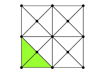
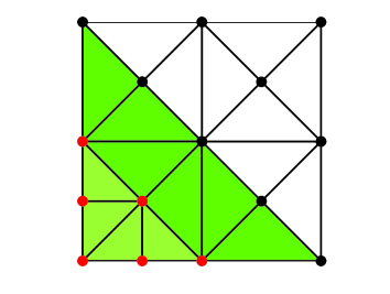
Figure 2. The left figure shows a mesh ${\mathcal{T}}_{\ell-1}$, where the two elements in the lower left corner are marked for refinement (green). Bisection of these two elements provides the mesh ${\mathcal{T}}_{\ell}$ (right), where two new nodes are created. The set $\widetilde{\mathcal{N}}_{\ell}$ consists of these new nodes plus their immediate neighbours (red). The union of the support of basis functions in $\widetilde{\mathcal{X}}^{\ell}={\rm span}\{\eta_{z}^{\ell}\,:\,z\in\widetilde{\mathcal{N}}_{\ell}\}$ is given by the light- and dark-green areas in the right figure.

2.5. Local multilevel diagonal preconditioner (LMLD)

For any $L\in{\mathbb{N}}_{0}$, we aim to derive a preconditioner $(\widetilde{\mathbf{B}}^{L})^{-1}$ for the Galerkin matrix $\mathbf{A}^{L}$ from (13) with respect to the space ${\mathcal{X}}^{L}$ and the basis $\big{\{}\eta_{z}^{L}\,:\,z\in{\mathcal{N}}_{L}\big{\}}$.

For all $0\leq\ell\leq L$, let $\widetilde{\mathbf{A}}^{\ell}$ be the Galerkin matrix with respect to $\widetilde{\mathcal{X}}^{\ell}$ and the associated basis $\big{\{}\eta_{z}^{\ell}\,:\,z\in\widetilde{\mathcal{N}}_{\ell}\big{\}}$. Let $\widetilde{\mathbf{D}}^{\ell}$ be the diagonal matrix $\widetilde{\mathbf{D}}^{\ell}_{jk}:=\widetilde{\mathbf{A}}^{\ell}_{jj}\delta_{jk}$ with Kronecker’s delta $\delta_{jk}$. Define $\widetilde{N}_{\ell}=\#\widetilde{\mathcal{N}}_{\ell}$ and $N_{L}=\#{\mathcal{N}}_{L}$. We consider the embedding $\widetilde{\mathcal{I}}^{\ell}:\widetilde{\mathcal{X}}^{\ell}\to{\mathcal{X}}^{L}$, i.e., the formal identity. Let $\widetilde{\bf I}^{\ell}\in{\mathbb{R}}^{N_{L}\times\widetilde{N}_{\ell}}$ be the matrix representation of the operator $\widetilde{\mathcal{I}}^{\ell}$ with respect to the bases of $\widetilde{\mathcal{X}}^{\ell}$ resp. ${\mathcal{X}}^{L}$. With this notation, we consider the matrix

(17) $$(\widetilde{\mathbf{B}}^{L})^{-1}=\sum_{\ell=0}^{L}\widetilde{\bf I}^{\ell}\,(\widetilde{\mathbf{D}}^{\ell})^{-1}(\widetilde{\bf I}^{\ell})^{T}.$$

Instead of solving $\mathbf{A}^{L}{\mathbf{x}}^{L}={\bf b}^{L}$, we now consider the preconditioned linear system

(18) $$(\widetilde{\mathbf{B}}^{L})^{-1}\mathbf{A}^{L}{\mathbf{x}}^{L}=(\widetilde{\mathbf{B}}^{L})^{-1}{\bf b}^{L}.$$

As is shown in Section 4.1, $(\widetilde{\mathbf{B}}^{L})^{-1}$ corresponds to a diagonal scaling on each local subspace $\widetilde{\mathcal{X}}^{\ell}$. Therefore, this type of preconditioner is called local multilevel diagonal scaling.

For a symmetric and positive definite matrix $\mathbf{C}\in{\mathbb{R}}^{N_{L}\times N_{L}}$, we denote by $\langle\cdot\,,\,\cdot\rangle_{\mathbf{C}}=\langle\mathbf{C}\cdot\,,\,\cdot\rangle_{2}$ the induced scalar product on ${\mathbb{R}}^{N_{L}}$, and by $\|\cdot\|_{\mathbf{C}}$ the corresponding norm resp. induced matrix norm. Here $\langle\cdot\,,\,\cdot\rangle_{2}$ denotes the Euclidean inner product on ${\mathbb{R}}^{N_{L}}$. We define the condition number ${\rm cond}_{\mathbf{C}}$ of a matrix $\mathbf{A}\in{\mathbb{R}}^{N_{L}\times N_{L}}$ as

(19) $${\rm cond}_{\mathbf{C}}(\mathbf{A}):=\|\mathbf{A}\|_{\mathbf{C}}\|\mathbf{A}^{-1}\|_{\mathbf{C}}.$$

The main result of this work reads as follows.

Theorem 1.

The matrix $(\widetilde{\mathbf{B}}^{L})^{-1}$ is symmetric and positive definite with respect to $\langle\cdot\,,\,\cdot\rangle_{2}$, and $\widetilde{\mathbf{P}}_{\rm AS}^{L}:=(\widetilde{\mathbf{B}}^{L})^{-1}\mathbf{A}^{L}$ is symmetric and positive definite with respect to $\langle\cdot\,,\,\cdot\rangle_{\widetilde{\mathbf{B}}^{L}}$. Moreover, the minimal and maximal eigenvalues of the matrix $\widetilde{\mathbf{P}}_{\rm AS}^{L}$ satisfy

(20) $$c\leq\lambda_{\rm min}(\widetilde{\mathbf{P}}_{\rm AS}^{L})\quad\text{and}\quad\lambda_{\rm max}(\widetilde{\mathbf{P}}_{\rm AS}^{L})\leq C,$$

where the constants $c,C>0$ depend only on $\Gamma$ and the initial triangulation ${\mathcal{T}}_{0}$. In particular, the condition number of the additive Schwarz matrix $\widetilde{\mathbf{P}}_{\rm AS}^{L}$ is $L$-independently bounded by

(21) $${\rm cond}_{\widetilde{\mathbf{B}}^{L}}(\widetilde{\mathbf{P}}_{\rm AS}^{L})\leq C/c.$$

The proof of Theorem 1 is given in Section 4 below, and we focus on the relevant application first: Consider an iterative solution method, such as the GMRES method [SS86] or the CG method [Saa03] to solve (18), where the relative reduction of the $j$-th residual depends only on the condition number ${\rm cond}_{\widetilde{\mathbf{B}}}(\widetilde{\mathbf{P}}_{\rm AS}^{L})$. Then, Theorem 1 proves that the iterative scheme, together with the preconditioner $\widetilde{\mathbf{B}}^{L}$ is efficient in the sense that the number of iterations to reduce the relative residual under the tolerance $\varepsilon$ is bounded by a constant that depends only on $\Gamma$, and the initial triangulation ${\mathcal{T}}_{0}$, but is completely independent of the current triangulation ${\mathcal{T}}_{L}$.

2.6. Global multilevel diagonal preconditioner (GMLD)

In addition to the new local multilevel diagonal preconditioner from Section 2.5, we consider a global multilevel diagonal preconditioner, where we use all nodes $z\in{\mathcal{N}}_{\ell}$ of the triangulation ${\mathcal{T}}_{\ell}$ instead of only $\widetilde{\mathcal{N}}_{\ell}$ to construct the preconditioner. Such an approach has, for instance, been investigated in [Mai09] for 2D hypersingular integral equations with graded meshes on an open curve. In the latter work it is proved that the maximal eigenvalue of the associated additive Schwarz operator is bounded up to some constant by $L^{2}$. With the new analytical tools developed here, we improve this estimate and show that the maximal eigenvalue can be bounded linearly in $L$. Our result holds for all $\gamma$-shape regular meshes on open and closed boundaries for $d=2,3$. Moreover, this bound is sharp, as it is confirmed in the numerical example from Section 3.2.

Let $\mathbf{A}^{\ell}$ denote the Galerkin matrix with respect to ${\mathcal{X}}^{\ell}$ and the basis $\{\eta_{z}^{\ell}\,:\,z\in{\mathcal{N}}_{\ell}\}$. We consider the diagonal $\mathbf{D}^{\ell}$ of this matrix, i.e. $\mathbf{D}_{jk}^{\ell}:=\delta_{jk}\mathbf{A}_{jj}^{\ell}$. Let $\mathcal{I}^{\ell}:{\mathcal{X}}^{\ell}\to{\mathcal{X}}^{L}$ denote the canonical embedding and let $\mathbf{I}^{\ell}$ denote its matrix representation with respect to the nodal basis of ${\mathcal{X}}^{\ell}$ and ${\mathcal{X}}^{L}$. We define the global multilevel preconditioner $(\mathbf{B}^{L})^{-1}$ by

(22) $$(\mathbf{B}^{L})^{-1}:=\sum_{\ell=0}^{L}\mathbf{I}^{\ell}(\mathbf{D}^{\ell})^{-1}(\mathbf{I}^{\ell})^{T}.$$

Theorem 2.

The matrix $(\mathbf{B}^{L})^{-1}$ is symmetric and positive definite with respect to $\langle\cdot\,,\,\cdot\rangle_{2}$, and $\mathbf{P}_{\rm AS}^{L}:=(\mathbf{B}^{L})^{-1}\mathbf{A}^{L}$ is symmetric and positive definite with respect to $\langle\cdot\,,\,\cdot\rangle_{\mathbf{B}^{L}}$. Moreover, the minimal and maximal eigenvalues of the matrix $\mathbf{P}_{\rm AS}^{L}$ satisfy

(23) $$c\leq\lambda_{\rm min}(\mathbf{P}_{\rm AS}^{L})\quad\text{and}\quad\lambda_{\rm max}(\mathbf{P}_{\rm AS}^{L})\leq C(L+1),$$

where the constants $c,C>0$ depend only on $\Gamma$ and the initial triangulation ${\mathcal{T}}_{0}$, but are independent of the level $L$. In particular, the condition number of the additive Schwarz matrix $\mathbf{P}_{\rm AS}^{L}$ is bounded by

(24) $${\rm cond}_{\mathbf{B}^{L}}(\mathbf{P}_{\rm AS}^{L})\leq(L+1)\,C/c.$$

3. Numerical examples

In this section we consider different 2D experiments to show the efficiency of the proposed local multilevel diagonal preconditioner $\widetilde{\mathbf{B}}^{L}$ from (18) numerically. In the first two experiments, we consider problems on the boundary of an L-shaped domain. In the last experiment, we consider a problem on the slit $\Gamma=(-1,1)\times\{0\}$. In both cases, the exact solution is known. Moreover, for the problems under considerations it is known, that uniform mesh-refinement will lead to suboptimal convergence rates, whereas adaptive refinement regains the optimal order of convergence. Thus, the use of adaptive methods is preferable.

For both examples, the mesh-adaptivity is driven by the ZZ-type error estimator proposed in [FFKP13]. The resulting linear systems are solved by GMRES. We compare the following preconditioners with respect to time, number of iterations, and condition numbers:

• LMLD local multilevel diagonal preconditioner from (18);

• GMLD global multilevel diagonal preconditioner from Section 2.6;

• HB hierarchical basis preconditioner, where only new nodes are considered for preconditioning [TSM97]: Define $\underline{{\mathcal{N}}}_{\ell}:={\mathcal{N}}_{\ell}\backslash{\mathcal{N}}_{\ell-1}$ as the set of new nodes and define $\underline{\mathbf{D}}^{\ell}$ as the diagonal matrix of the Galerkin matrix with respect to the space $\underline{{\mathcal{X}}}^{\ell}:=\{\eta_{z}^{\ell}\,:\,z\in\underline{{\mathcal{N}}}_{\ell}\}$. Let $\underline{\mathcal{I}}^{\ell}:\underline{{\mathcal{X}}}^{\ell}\to{\mathcal{X}}^{L}$ denote the canonical embedding with matrix representation $\underline{\mathbf{I}}^{\ell}$. The hierarchical basis preconditioner is then given by

  (25) $$\mathbf{B}_{\rm HB}^{L}:=\sum_{\ell=0}^{L}\underline{\mathbf{I}}^{\ell}(\underline{\mathbf{D}}^{\ell})^{-1}(\underline{\mathbf{I}}^{\ell})^{T}.$$

  The preconditioned matrix reads $\mathbf{P}_{\rm HB}^{L}:=(\mathbf{B}_{\rm HB}^{L})^{-1}\mathbf{A}^{L}$.

• DIAG diagonal scaling of the Galerkin matrix [AMT99, GM06]. The preconditioned matrix reads $\mathbf{P}_{\rm diag}^{L}:=(\mathbf{D}^{L})^{-1}\mathbf{A}^{L}$.

\psfrag{x}{\tiny$x$}\psfrag{y}{\tiny$y$}\includegraphics[width=260.17464pt]{figures/Lshape}

Figure 3. L-shaped domain $\Omega$ and initial triangulation ${\mathcal{T}}_{0}$ with $\#{\mathcal{T}}_{0}=8$.

\psfrag{number of elements}[c][c]{\tiny number of elements $N$}\psfrag{condition numbers}[c][c]{\tiny condition numbers}\psfrag{OS}[0][-145]{\tiny${\mathcal{O}}(N\log(Nh_{{\rm min},L})$}\psfrag{O1}{\tiny${\mathcal{O}}(1)$}\includegraphics[width=260.17464pt]{figures/cond_10277}

Figure 4. Condition numbers $\lambda_{\rm max}/\lambda_{\rm min}$ of the preconditioned Galerkin matrices $\widetilde{\mathbf{P}}_{\rm AS}^{L}$ (LMLD), $\mathbf{P}_{\rm AS}^{L}$ (GMLD), $\mathbf{P}_{\rm HB}^{L}$ (HB), $\mathbf{P}_{\rm diag}^{L}$ (DIAG), and the unpreconditioned matrix $\mathbf{A}^{L}$ (A) for the problem from Section 3.1.

\psfrag{number of elements}[c][c]{\tiny number of elements $N$}\psfrag{time}[c][c]{\tiny time [sec.]}\psfrag{ON}{\tiny${\mathcal{O}}(N)$}\psfrag{ON2}{\tiny${\mathcal{O}}(N^{2})$}\includegraphics[width=260.17464pt]{figures/time_10277}

Figure 5. Computational times for GMRES algorithm to reduce relative residual under the bound $\varepsilon=10^{-8}$ for the problem from Section 3.1 and the preconditioned Galerkin systems $\widetilde{\mathbf{P}}_{\rm AS}^{L}$ (LMLD), $\mathbf{P}_{\rm AS}^{L}$ (GMLD), $\mathbf{P}_{\rm HB}^{L}$ (HB), $\mathbf{P}_{\rm diag}^{L}$ (DIAG). DIRECT stands for the direct solver.

\psfrag{number of elements}[c][c]{\tiny number of elements $N$}\psfrag{iterations}[c][c]{\tiny number of iterations}\includegraphics[width=260.17464pt]{figures/iter_10277}

Figure 6. Number of iterations of GMRES to reduce relative residual under the bound $\varepsilon=10^{-8}$ for the problem from Section 3.1 and the preconditioned Galerkin systems $\widetilde{\mathbf{P}}_{\rm AS}^{L}$ (LMLD), $\mathbf{P}_{\rm AS}^{L}$ (GMLD), $\mathbf{P}_{\rm HB}^{L}$ (HB), $\mathbf{P}_{\rm diag}^{L}$ (DIAG).

\psfrag{number of elements}[c][c]{\tiny number of elements $N$}\psfrag{condition numbers}[c][c]{\tiny condition numbers}\psfrag{OS}{\tiny${\mathcal{O}}(N\log(Nh_{{\rm min},L}))$}\psfrag{O1}{\tiny${\mathcal{O}}(1)$}\psfrag{OL}{\tiny${\mathcal{O}}(L)$}\psfrag{OL2}{\tiny${\mathcal{O}}(L^{2})$}\includegraphics[width=260.17464pt]{figures/cond_altLshape}

Figure 7. Condition numbers $\lambda_{\rm max}/\lambda_{\rm min}$ of the preconditioned Galerkin matrices $\widetilde{\mathbf{P}}_{\rm AS}^{L}$ (LMLD), $\mathbf{P}_{\rm AS}^{L}$ (GMLD), $\mathbf{P}_{\rm HB}^{L}$ (HB), $\mathbf{P}_{\rm diag}^{L}$ (DIAG), and the unpreconditioned matrix $\mathbf{A}^{L}$ (A) for the problem from Section 3.2.

\psfrag{number of elements}[c][c]{\tiny number of elements $N$}\psfrag{condition numbers}[c][c]{\tiny condition numbers}\psfrag{OS}[0][-145]{\tiny${\mathcal{O}}(N\log(Nh_{{\rm min},L}))$}\psfrag{O1}{\tiny${\mathcal{O}}(1)$}\includegraphics[width=260.17464pt]{figures/cond_slit_5374}

Figure 8. Condition numbers $\lambda_{\rm max}/\lambda_{\rm min}$ of the preconditioned Galerkin matrices $\widetilde{\mathbf{P}}_{\rm AS}^{L}$ (LMLD), $\mathbf{P}_{\rm AS}^{L}$ (GMLD), $\mathbf{P}_{\rm HB}^{L}$ (HB), $\mathbf{P}_{\rm diag}^{L}$ (DIAG), and the unpreconditioned matrix $\mathbf{A}^{L}$ (A) for the problem from Section 3.3.

\psfrag{number of elements}[c][c]{\tiny number of elements $N$}\psfrag{time}[c][c]{\tiny time [sec.]}\psfrag{ON}{\tiny${\mathcal{O}}(N)$}\psfrag{ON2}{\tiny${\mathcal{O}}(N^{2})$}\includegraphics[width=260.17464pt]{figures/time_slit_5374}

Figure 9. Computational times for GMRES algorithm to reduce relative residual under the bound $\varepsilon=10^{-8}$ for the problem from Section 3.3 and the preconditioned Galerkin systems $\widetilde{\mathbf{P}}_{\rm AS}^{L}$ (LMLD), $\mathbf{P}_{\rm AS}^{L}$ (GMLD), $\mathbf{P}_{\rm HB}^{L}$ (HB), $\mathbf{P}_{\rm diag}^{L}$ (DIAG). DIRECT stands for the direct solver.

\psfrag{number of elements}[c][c]{\tiny number of elements $N$}\psfrag{iterations}[c][c]{\tiny number of iterations}\includegraphics[width=260.17464pt]{figures/iter_slit_5374}

Figure 10. Number of iterations of GMRES to reduce relative residual under the bound $\varepsilon=10^{-8}$ for the problem from Section 3.3 and the preconditioned Galerkin systems $\widetilde{\mathbf{P}}_{\rm AS}^{L}$ (LMLD), $\mathbf{P}_{\rm AS}^{L}$ (GMLD), $\mathbf{P}_{\rm HB}^{L}$ (HB), $\mathbf{P}_{\rm diag}^{L}$ (DIAG).

The preconditioners GMLD and HB are very similar to LMLD, but lack effectivity, i.e., the condition number depends on the level $L$ resp. on the mesh-width function $h_{L}$. Since the diagonal elements of the matrix $\mathbf{A}^{L}$ are essentially constant, the simple diagonal preconditioner has no significant effect on the condition numbers, see also [AMT99]. Moreover, the GMRES-based iterative solution is compared to a direct solver DIRECT for the unpreconditioned system.

All computations were performed with MATLAB (2012b) on an Intel Core i7-3930K machine with 32GB RAM under a x86_64 GNU/Linux system. For the GMRES algorithm, we use the MATLAB function gmres.m. For the direct solver, we use the MATLAB backslash operator. The assembly of the boundary integral operators was done with help of the MATLAB BEM-library HILBERT [AEF⁺11].

3.1. Adaptive BEM for hypersingular integral equation for 2D Neumann problem on L-shaped domain

We consider the boundary $\Gamma=\partial\Omega$ of the L-shaped domain $\Omega$, sketched in Figure 3. With the 2D polar coordinates $(r,\varphi)$ of $x\in{\mathbb{R}}^{2}\backslash\{0\}$, the function

$$w(x,y)=r^{2/3}\cos(2/3\varphi),$$

satisfies the Neumann problem

$$-\Delta w=0\text{ in }\Omega,\quad\text{and}\quad\partial_{n}w=:\phi\text{ on }\Gamma.$$

With the adjoint double-layer potential, we define the right-hand side $f$ of (1) as

$$f=(1/2-\mathcal{K}^{\prime})\partial_{\boldsymbol{n}}w.$$

The exact solution $u$ of (1) is, up to some additive constant, the trace $u=w|_{\Gamma}$ of the potential $w$. We use the adaptive lowest-order BEM from [FFKP13] to approximate $u$. This leads to successively refined meshes ${\mathcal{T}}_{\ell}$ for $\ell=0,1,2\dots$.

In Figure 4, we compare the condition numbers of the different preconditioned matrices and the Galerkin matrix $\mathbf{A}^{L}$, i.e., the ratio between maximal and minimal eigenvalue. As predicted by Theorem 1, the condition number of the preconditioned matrix $\widetilde{\mathbf{P}}_{\rm AS}^{L}$ stays bounded, whereas the preconditioned systems which use GMLD resp. HB, are suboptimal. The condition numbers of the unpreconditioned system DIRECT as well as the diagonally preconditioned system DIAG essentially coincide.

If we compare the computational times used for solving the different preconditioned systems, we infer that the system with the matrix $\widetilde{\mathbf{P}}_{\rm AS}^{L}$ is solved fastest, see Figure 5. Clearly, this is because the number of iterations, is the smallest of all iterative methods, cf. Figure 6. We obtain from Figure 5 that the computational time is almost linear in the number of elements in the mesh ${\mathcal{T}}_{L}$. However, direct solvers are known to have higher computational costs. Moreover, the memory consumption of direct solvers also exceeds that of an efficient iterative solution method. Therefore, if the number of elements are large, efficient iterative methods are inevitable.

3.2. Artificial mesh-adaptation for hypersingular integral equation for 2D Neumann problem on L-shaped domain

We consider again the problem from the previous Section 3.1. However, we use a stronger mesh-adaptation towards the reentrant corner: We start with the initial mesh ${\mathcal{T}}_{0}$ as given in Figure 3, and obtain ${\mathcal{T}}_{\ell}$ from ${\mathcal{T}}_{\ell-1}$ by bisecting only the two elements closest to the origin $(0,0)$. Note that this refinement preserves $\gamma$-shape regularity of the triangulations ${\mathcal{T}}_{\ell}$. Simple calculations show $h_{{\rm min},\ell}=2^{-\ell}h_{0}$ and $h_{{\rm max},\ell}=h_{0}$, where $h_{0}\in{\mathbb{R}}$ denotes the constant mesh-width of the initial triangulation. We compare the condition numbers of the unpreconditioned and preconditioned systems in Figure 7. Here, we consider LMLD, GMLD, and HB, as well as the simple diagonal scaling DIAG. The results from Figure 7 show that the condition number of $\widetilde{\mathbf{P}}_{\rm AS}^{L}$ is uniformly bounded, while the condition number of $\mathbf{P}_{\rm AS}^{L}$ grows with $L$. In particular, this proves that Theorem 1 and 2 are sharp. The condition number of $\mathbf{P}_{\rm HB}^{L}$ grows even worse. It is proved in [TSM97, Corollary 1] that the condition number of HB is bounded by $|\log(h_{{\rm min},L})|^{2}\simeq L^{2}$.

3.3. Problem on slit

We consider the hypersingular equation (1) on the slit $\Gamma=(-1,1)\times\{0\}$ with right-hand side $f=1$ and exact solution $u(x,0)=2\sqrt{1-x^{2}}$. For this example, the correct energy space is $\widetilde{H}^{1/2}(\Gamma)$, and the exact solution belongs to $u\in(\widetilde{H}^{1/2}(\Gamma)\cap H^{1-\varepsilon}(\Gamma))\backslash H^{1}(\Gamma)$ for all $\varepsilon>0$. In particular, uniform mesh-refinement thus leads to the reduced order of convergence ${\mathcal{O}}(h^{1/2})={\mathcal{O}}(N^{-1/2})$, while the adaptive mesh-refinement of [FFKP13] regains the optimal order ${\mathcal{O}}(N^{-3/2})$.

As is shown in Section 6 below, the main result of Theorem 1 also holds in this setting. We compare different types of multilevel additive Schwarz preconditioners like LMLD, GMLD, and HB, as well as simple diagonal scaling with respect to condition numbers in Figure 8 resp. the number of GMRES iterations in Figure 10. Moreover, we also compare GMRES vs. the direct solver with respect to the computational time, see Figure 9.

4. Proof of Theorem 1

4.1. Abstract analysis of additive Schwarz operators

In this subsection, we show that the multilevel diagonal scaling from Section 2 is a multilevel additive Schwarz method. Recall the notation from Section 2.4 and Section 2.5.

For each subspace ${\mathcal{X}}_{z}^{\ell}={\rm span}\{\eta_{z}^{\ell}\}$, we define the projection $\mathcal{P}_{z}^{\ell}:{\mathcal{X}}^{L}\to{\mathcal{X}}_{z}^{\ell}$ by

(26) $$\langle\langle\mathcal{P}_{z}^{\ell}v\,,\,w_{z}^{\ell}\rangle\rangle=\langle\langle v\,,\,w_{z}^{\ell}\rangle\rangle\quad\text{for all }w_{z}^{\ell}\in{\mathcal{X}}_{z}^{\ell}.$$

Note that $\mathcal{P}_{z}^{\ell}$ is the orthogonal projection onto the one-dimensional space ${\mathcal{X}}_{z}^{\ell}$. Thus, the explicit representation of $\mathcal{P}_{z}^{\ell}$ reads

(27) $$\mathcal{P}_{z}^{\ell}v=\frac{\langle\langle v\,,\,\eta_{z}^{\ell}\rangle\rangle}{|||\eta_{z}^{\ell}|||^{2}}\,\eta_{z}^{\ell}.$$

Based on $\mathcal{P}_{z}^{\ell}$, we define the additive Schwarz operator

(28) $$\widetilde{\mathcal{P}}_{\rm AS}^{L}:=\sum_{\ell=0}^{L}\sum_{z\in\widetilde{\mathcal{N}}_{\ell}}\mathcal{P}_{z}^{\ell}:{\mathcal{X}}^{L}\to{\mathcal{X}}^{L}.$$

Let $v=\sum_{j=1}^{N_{L}}{\mathbf{x}}_{j}\eta_{z_{j}}^{L}$, $w=\sum_{k=1}^{\widetilde{N}_{\ell}}{\mathbf{y}}_{k}\eta_{z_{k}}^{\ell}$. A moment’s reflection reveals that the operator

(29) $$\widetilde{\mathcal{P}}^{\ell}:=\sum_{z\in\widetilde{\mathcal{N}}_{\ell}}\mathcal{P}_{z}^{\ell}:{\mathcal{X}}^{L}\to\widetilde{\mathcal{X}}^{\ell}$$

and the matrix

(30) $$\widetilde{\mathbf{P}}^{\ell}=(\widetilde{\mathbf{D}}^{\ell})^{-1}(\widetilde{\bf I}^{\ell})^{T}\mathbf{A}^{L}$$

are related through $\langle\langle\widetilde{\mathcal{P}}^{\ell}v\,,\,w\rangle\rangle=\langle\widetilde{\mathbf{P}}^{\ell}{\mathbf{x}}\,,\,{\mathbf{y}}\rangle_{\mathbf{A}^{L}}$. In particular, the matrix $\widetilde{\mathbf{P}}_{\rm AS}^{L}$ reads

(31) $$\widetilde{\mathbf{P}}_{\rm AS}^{L}=\Big{(}\sum_{\ell=0}^{L}\widetilde{\bf I}^{\ell}(\widetilde{\mathbf{D}}^{\ell})^{-1}(\widetilde{\bf I}^{\ell})^{T}\Big{)}\mathbf{A}^{L}=:(\mathbf{B}^{L})^{-1}\mathbf{A}^{L},$$

with $\langle\langle\widetilde{\mathcal{P}}_{\rm AS}^{L}v\,,\,w\rangle\rangle=\langle\widetilde{\mathbf{P}}_{\rm AS}^{L}{\mathbf{x}}\,,\,{\mathbf{y}}\rangle_{\mathbf{A}^{L}}$ for $w=\sum_{k=0}^{N_{L}}{\mathbf{y}}_{k}\eta_{z_{k}}^{L}$, i.e. the additive Schwarz operator $\widetilde{\mathcal{P}}_{\rm AS}^{L}$ generates the preconditioner from Theorem 1.

The following well-known result, see e.g. [GO94, Lemma 2], collects some soft results on the additive Schwarz operator $\widetilde{\mathcal{P}}_{\rm AS}^{L}$ which hold in an arbitrary Hilbert space setting with

(32) $${\mathcal{X}}^{L}=\sum_{\ell=0}^{L}\sum_{z\in\widetilde{\mathcal{N}}_{\ell}}{\mathcal{X}}_{z}^{\ell}.$$

Lemma 3.

The operator $\widetilde{\mathcal{P}}_{\rm AS}^{L}$ is linear and bounded as well as symmetric

(33) $$\langle\langle\widetilde{\mathcal{P}}_{\rm AS}^{L}v\,,\,w\rangle\rangle=\langle\langle v\,,\,\widetilde{\mathcal{P}}_{\rm AS}^{L}w\rangle\rangle\quad\text{for all }v,w\in H^{1/2}(\Gamma)$$

and positive definite on ${\mathcal{X}}^{L}$

(34) $$\langle\langle\widetilde{\mathcal{P}}_{\rm AS}^{L}v\,,\,v\rangle\rangle>0\quad\text{for all }v\in{\mathcal{X}}^{L}\backslash\{0\}$$

with respect to the scalar product $\langle\langle\cdot\,,\,\cdot\rangle\rangle$.∎

In our concrete setting, the additive Schwarz operator $\widetilde{\mathcal{P}}_{\rm AS}^{L}$ satisfies the following spectral equivalence estimate which is proved in Section 4.5 (lower bound) resp. Section 4.6 (upper bound).

Proposition 4.

The operator $\widetilde{\mathcal{P}}_{\rm AS}^{L}$ satisfies

(35) $$c\,|||v|||^{2}\leq\langle\langle\widetilde{\mathcal{P}}_{\rm AS}^{L}v\,,\,v\rangle\rangle\leq C\,|||v|||^{2}\quad\text{for all }v\in{\mathcal{X}}^{L}.$$

The constants $c,C>0$ depend only on $\Gamma$ and the initial triangulation ${\mathcal{T}}_{0}$.

The relation between $\widetilde{\mathcal{P}}_{\rm AS}^{L}$ and the symmetric matrix $\widetilde{\mathbf{P}}_{\rm AS}^{L}$ yields the eigenvalue estimates from Theorem 1.

Proof of Theorem 1.

Symmetry of $(\widetilde{\mathbf{B}}^{L})^{-1}$ follows from the definition (17). The other properties are obtained using the identity

$$\langle\langle\widetilde{\mathcal{P}}_{\rm AS}^{L}v\,,\,w\rangle\rangle=\langle\widetilde{\mathbf{P}}_{\rm AS}^{L}{\mathbf{x}}\,,\,{\mathbf{y}}\rangle_{\mathbf{A}^{L}}\quad\text{for all }v=\sum_{j=1}^{N_{L}}{\mathbf{x}}_{j}\eta_{z_{j}}^{L},w=\sum_{j=1}^{N_{L}}{\mathbf{y}}_{j}\eta_{z_{j}}^{L}.$$

An immediate consequence of this identity and Lemma 3 is symmetry as well as positive definiteness of $\widetilde{\mathbf{P}}_{\rm AS}^{L}$ with respect to $\langle\cdot\,,\,\cdot\rangle_{\mathbf{A}^{L}}$. Proposition 4 directly yields

$$c\|{\mathbf{x}}\|_{\mathbf{A}^{L}}^{2}\leq\langle\widetilde{\mathbf{P}}_{\rm AS}^{L}{\mathbf{x}}\,,\,{\mathbf{x}}\rangle_{\mathbf{A}^{L}}\leq C\|{\mathbf{x}}\|_{\mathbf{A}^{L}}^{2}\quad\text{for all }{\mathbf{x}}\in{\mathbb{R}}^{N_{L}}.$$

Thus, a bound for the minimal resp. maximal eigenvalue of $\widetilde{\mathbf{P}}_{\rm AS}^{L}$ is given by

$$\lambda_{\rm min}(\widetilde{\mathbf{P}}_{\rm AS}^{L})\geq c,\qquad\lambda_{\rm max}(\widetilde{\mathbf{P}}_{\rm AS}^{L})\leq C.$$

In the next step, we prove positive definiteness of $(\widetilde{\mathbf{B}}^{L})^{-1}$. Lemma 3 shows

$$0<\langle\langle\widetilde{\mathcal{P}}_{\rm AS}^{L}v\,,\,v\rangle\rangle=\langle\widetilde{\mathbf{P}}_{\rm AS}^{L}{\mathbf{x}}\,,\,{\mathbf{x}}\rangle_{\mathbf{A}^{L}}=\langle(\widetilde{\mathbf{B}}^{L})^{-1}\mathbf{A}^{L}{\mathbf{x}}\,,\,\mathbf{A}^{L}{\mathbf{x}}\rangle_{2}.$$

Since $\mathbf{A}^{L}$ is regular, we obtain $\langle(\widetilde{\mathbf{B}}^{L})^{-1}{\mathbf{y}}\,,\,{\mathbf{y}}\rangle_{2}>0$ for all ${\mathbf{y}}\in{\mathbb{R}}^{N_{L}}$. In particular the inverse $\widetilde{\mathbf{B}}^{L}$ of $(\widetilde{\mathbf{B}}^{L})^{-1}$ is well-defined, symmetric and positive definite. The identity

$$\langle\widetilde{\mathbf{P}}_{\rm AS}^{L}{\mathbf{x}}\,,\,{\mathbf{y}}\rangle_{\widetilde{\mathbf{B}}^{L}}=\langle\mathbf{A}^{L}{\mathbf{x}}\,,\,{\mathbf{y}}\rangle_{2}\quad\text{for all }{\mathbf{x}},{\mathbf{y}}\in{\mathbb{R}}^{N_{L}},$$

and the symmetry of $\mathbf{A}^{L}$ prove that $\widetilde{\mathbf{P}}_{\rm AS}^{L}$ is symmetric with respect to $\langle\cdot\,,\,\cdot\rangle_{\widetilde{\mathbf{B}}^{L}}$. Finally, we stress that the condition number ${\rm cond}_{\mathbf{C}}(\mathbf{A})$ of a matrix $\mathbf{A}$ is given by ${\rm cond}_{\mathbf{C}}(\mathbf{A})=\lambda_{\rm max}(\mathbf{A})/\lambda_{\rm min}(\mathbf{A})$, if $\mathbf{C}$ is positive definite as well as symmetric and $\mathbf{A}$ is symmetric with respect to $\langle\cdot\,,\,\cdot\rangle_{\mathbf{C}}$. Therefore,

$${\rm cond}_{\widetilde{\mathbf{B}}^{L}}(\widetilde{\mathbf{P}}_{\rm AS}^{L})={\rm cond}_{\mathbf{A}^{L}}(\widetilde{\mathbf{P}}_{\rm AS}^{L})=\frac{\lambda_{\rm max}(\widetilde{\mathbf{P}}_{\rm AS}^{L})}{\lambda_{\rm min}(\widetilde{\mathbf{P}}_{\rm AS}^{L})}\leq\frac{C}{c},$$

which also concludes the proof. ∎

The remainder of this section is now concerned with the proof of Proposition 4. This requires some preparations and auxiliary results (Section 4.2–4.4), before we face the lower bound (Section 4.5) and the upper bound (Section 4.6) of (35).

4.2. Uniform mesh-refinement and $L^{2}$-orthogonal projection

Besides the sequence of locally refined triangulations ${\mathcal{T}}_{\ell}$, we consider a second unrelated sequence $\widehat{\mathcal{T}}_{m}$ of uniform triangulations: Let $\widehat{\mathcal{T}}_{0}:={\mathcal{T}}_{0}$ and let $\widehat{\mathcal{T}}_{m+1}$ be obtained from $\widehat{\mathcal{T}}_{m}$ by uniform refinement, i.e. all elements of $\widehat{\mathcal{T}}_{m}$ are bisected into son elements with half diameter. For $d=2$, this corresponds to one bisection per element, while three bisections are used for $d=3$, cf. Figure 1. Let $\widehat{\mathcal{N}}_{m}$ denote the set of all nodes of $\widehat{\mathcal{T}}_{m}$. Recall $\widehat{h}_{0}:=\max_{T\in{\mathcal{T}}_{0}}h_{0}(T)$ and define the constant

(36) $$\widehat{h}_{m}:=2^{-m}\widehat{h}_{0}\quad\text{for each }m\geq 1.$$

Note that $\widehat{h}_{m}$ is equivalent to the usual local mesh-size function on $\widehat{\mathcal{T}}_{m}$, i.e. $\widehat{h}_{m}\simeq{\rm diam}(T)$ for all $T\in\widehat{\mathcal{T}}_{m}$ and all $m\geq 0$. For later use, we recall the following result which is part of [WC06, Proof of Lemma 3.3].

Lemma 5.

For all $z\in{\mathcal{N}}_{\ell}$ holds $z\in\widehat{\mathcal{N}}_{{\rm level}_{\ell}(z)}$ with

(37) $$C_{\ref{consteq_unif_1}}\widehat{h}_{{\rm level}_{\ell}(z)}\leq h_{\ell}(z)\leq C_{\ref{consteq_unif_2}}\widehat{h}_{{\rm level}_{\ell}(z)},$$

where the constants $C_{\ref{consteq_unif_1}},C_{\ref{consteq_unif_2}}>0$ depend only on the $\gamma$-shape regularity and the initial triangulation ${\mathcal{T}}_{0}$.∎

Let $\widehat{\mathcal{X}}^{m}:=\SS^{1}(\widehat{\mathcal{T}}_{m})$ and denote by $\widehat{\Pi}_{m}:L^{2}(\Gamma)\to\widehat{\mathcal{X}}^{m}$ the $L^{2}$-orthogonal projection onto $\widehat{\mathcal{X}}^{m}$.

Lemma 6.

For all $v\in H^{1/2}(\Gamma)$ holds

(38) $$\sum_{m=0}^{\infty}\widehat{h}_{m}^{-1}\|v-\widehat{\Pi}_{m}v\|_{L^{2}(\Gamma)}^{2}\leq C_{\rm norm}\,\|v\|_{H^{1/2}(\Gamma)}^{2}.$$

The constant $C_{\rm norm}>0$ depends only on $\Gamma$ and the initial triangulation ${\mathcal{T}}_{0}$.

Proof.

We note that $\widehat{\mathcal{X}}_{k}\subseteq\widehat{\mathcal{X}}_{k+1}$ and $\lim\limits_{k\to\infty}\|v-\widehat{\Pi}_{k}v\|_{L^{2}(\Gamma)}=0$ for all $v\in L^{2}(\Gamma)$. Thus,

(39) $$\|v-\widehat{\Pi}_{m}v\|_{L^{2}(\Gamma)}^{2}=\sum_{k=m+1}^{\infty}\|(\widehat{\Pi}_{k}-\widehat{\Pi}_{k-1})v\|_{L^{2}(\Gamma)}^{2}.$$

Plugging (39) into the left-hand side of (38) and changing the order of summation, we see

(40) $$\begin{split}\sum_{m=0}^{\infty}\widehat{h}_{m}^{-1}\|v-\widehat{\Pi}_{m}v\|_{L^{2}(\Gamma)}^{2}&=\sum_{m=0}^{\infty}\widehat{h}_{m}^{-1}\sum_{k=m+1}^{\infty}\|(\widehat{\Pi}_{k}-\widehat{\Pi}_{k-1})v\|_{L^{2}(\Gamma)}^{2}\\ &=\sum_{k=1}^{\infty}\Big{(}\sum_{m=0}^{k-1}\widehat{h}_{m}^{-1}\Big{)}\|(\widehat{\Pi}_{k}-\widehat{\Pi}_{k-1})v\|_{L^{2}(\Gamma)}^{2}.\end{split}$$

With the definition (36) of $\widehat{h}_{m}$ and the geometric series we infer

(41) $$\sum_{m=0}^{k-1}\widehat{h}_{m}^{-1}=\widehat{h}_{0}^{-1}\sum_{m=0}^{k-1}2^{m}<\widehat{h}_{0}^{-1}2^{k}=\widehat{h}_{k}^{-1}.$$

[AM03, Theorem 5] states that for $s\in[0,1]$ and $v\in H^{s}(\Gamma)$ it holds

(42) $$\|v\|_{H^{s}(\Gamma)}^{2}\simeq\|\widehat{\Pi}_{0}v\|_{H^{s}(\Gamma)}^{2}+\sum_{k=1}^{\infty}\widehat{h}_{k}^{-2s}\|(\widehat{\Pi}_{k}-\widehat{\Pi}_{k-1})v\|_{L^{2}(\Gamma)}^{2}.$$

The hidden constants in (42) depend only on $\Gamma$, the initial triangulation ${\mathcal{T}}_{0}$, and on $s$. Using equations (40)–(41) and norm equivalence (42) for $s=1/2$, we conclude the proof of (38). ∎

4.3. Scott-Zhang projection

We require a variant of the Scott-Zhang quasi-interpolation operator [SZ90], see also [AFF⁺13b] for higher-order polynomials $\SS^{p}({\mathcal{T}}_{\ell})$ for $p\geq 1$ and $H^{s}(\Gamma)$ resp. $\widetilde{H}^{s}(\Gamma)$ with $\Gamma\subseteq\partial\Omega$: For $z\in{\mathcal{N}}_{\ell}$, let $T_{z}^{\ell}\in{\mathcal{T}}_{\ell}$ be an element with $z\in T_{z}^{\ell}$. Let $\psi_{z}^{\ell}$ denote the $L^{2}$-dual basis function with

(43) $$\int_{T_{z}^{\ell}}\psi_{z}^{\ell}(x)\eta_{z^{\prime}}^{\ell}(x)\,ds_{x}=\delta_{zz^{\prime}}\quad\text{for all }z^{\prime}\in{\mathcal{N}}_{\ell}.$$

Then, the operator $J_{\ell}:L^{2}(\Gamma)\to\SS^{1}({\mathcal{T}}_{\ell})$ defined by

(44) $$J_{\ell}v=\sum_{z\in{\mathcal{N}}_{\ell}}\eta_{z}^{\ell}\int_{T_{z}^{\ell}}\psi_{z}^{\ell}(x)v(x)\,ds_{x}\quad\text{for all }v\in L^{2}(\Gamma),$$

is an $H^{s}$-stable projection onto $\SS^{1}({\mathcal{T}}_{\ell})$, i.e.

(45) $$J_{\ell}v_{\ell}=v_{\ell}\quad\text{and}\quad\|J_{\ell}v\|_{H^{s}(\Gamma)}\leq C_{\ref{conststable}}\,\|v\|_{H^{s}(\Gamma)}\quad\text{for all }v_{\ell}\in\SS^{1}({\mathcal{T}}_{\ell})\text{ and }v\in H^{s}(\Gamma).$$

Arguing as in [SZ90], $J_{\ell}$ satisfies for all $v\in H^{1}(\Gamma)$

(46) $$\|\nabla J_{\ell}v\|_{L^{2}(T)}\leq C_{\ref{constsz}}\,\|\nabla v\|_{L^{2}(\omega_{\ell}(T))}\quad\text{and}\quad\|v-J_{\ell}v\|_{L^{2}(T)}\leq C_{\ref{constsz}}\,h_{\ell}(T)\,\|\nabla v\|_{L^{2}(\omega_{\ell}(T))}.$$

The constant $C_{\ref{constsz}}>0$ depends only on $\gamma$-shape regularity of ${\mathcal{T}}_{\ell}$, while $C_{\ref{conststable}}>0$ additionally depends on $\Gamma$. Moreover, if $v$ is linear on $T_{z}^{\ell}$ it holds

(47) $$J_{\ell}v(z)=v(z).$$

Note that the choice of $T_{z}^{\ell}$ is arbitrary, but for $z\in{\mathcal{N}}_{\ell}\backslash\widetilde{\mathcal{N}}_{\ell}\subseteq{\mathcal{N}}_{\ell-1}$ we require that $T_{z}^{\ell-1}=T_{z}^{\ell}\in{\mathcal{T}}_{\ell}\cap{\mathcal{T}}_{\ell-1}$. For $z\in{\mathcal{N}}_{\ell}\backslash\widetilde{\mathcal{N}}_{\ell}$, it thus follows $\eta_{z}^{\ell}=\eta_{z}^{\ell-1}$ as well as $T_{z}^{\ell}=T_{z}^{\ell-1}$ and consequently $\psi_{z}^{\ell}=\psi_{z}^{\ell-1}$. This yields the following important property that allows us to construct a stable subspace decomposition:

(48) $$(J_{\ell}-J_{\ell-1})v(z)=0\quad\text{for all }z\in{\mathcal{N}}_{\ell}\backslash\widetilde{\mathcal{N}}_{\ell}.$$

In particular, we have

(49) $$(J_{\ell}-J_{\ell-1})v\in{\rm span}\{\eta_{z}^{\ell}\,:\>z\in\widetilde{\mathcal{N}}_{\ell}\}=\widetilde{\mathcal{X}}^{\ell}.$$

Finally and with the second-order node patch from (9), we have the following pointwise estimate for the Scott-Zhang projection.

Lemma 7.

For all $v\in L^{2}(\Gamma)$, it holds

(50) $$|(J_{\ell}-J_{\ell-1})v(z)|\leq C_{\ref{constsz:point}}\,h_{\ell}(z)^{-(d-1)/2}\|v\|_{L^{2}(\omega_{\ell-1}^{2}(z))}\quad\text{for all }z\in\widetilde{\mathcal{N}}_{\ell}.$$

The constant $C_{\ref{constsz:point}}>0$ depends only on $\gamma$-shape regularity of ${\mathcal{T}}_{\ell}$.

Proof.

According to [SZ90, Lemma 3.1], it holds $\|\psi_{z}^{\ell}\|_{L^{\infty}(T_{z}^{\ell})}\lesssim|T_{z}^{\ell}|^{-1}$. For any node $z\in\widetilde{\mathcal{N}}_{\ell}$, we have $T_{z}^{\ell}\subseteq\omega_{\ell}(z)\subseteq\omega_{\ell-1}^{2}(z)$ and thus

(51) $$\begin{split}|J_{\ell}v(z)|&\leq\int_{T_{z}^{\ell}}|\psi_{z}^{\ell}(x)v(x)|\,ds_{x}\leq\|\psi_{z}^{\ell}\|_{L^{\infty}(T_{z}^{\ell})}|T_{z}^{\ell}|^{1/2}\|v\|_{L^{2}(T_{z}^{\ell})}\\ &\lesssim|T_{z}^{\ell}|^{-1/2}\|v\|_{L^{2}(\omega_{\ell-1}^{2}(z))}\lesssim h_{\ell}(z)^{-(d-1)/2}\|v\|_{L^{2}(\omega_{\ell-1}^{2}(z))}.\end{split}$$

For $z\in\widetilde{\mathcal{N}}_{\ell}\backslash{\mathcal{N}}_{\ell-1}$, there exist two nodes $z_{1},z_{2}\in{\mathcal{N}}_{\ell-1}$ such that

$$J_{\ell-1}v(z)=\eta_{z_{1}}^{\ell-1}(z)\int_{T_{z_{1}}^{\ell-1}}\psi_{z_{1}}^{\ell-1}(x)v(x)\,ds_{x}+\eta_{z_{2}}^{\ell-1}(z)\int_{T_{z_{2}}^{\ell-1}}\psi_{z_{2}}^{\ell-1}(x)v(x)\,ds_{x}.$$

For $z\in\widetilde{\mathcal{N}}_{\ell}\cap{\mathcal{N}}_{\ell-1}$, this equality is understood with $z_{1}=z$ and $\eta_{z_{2}}^{\ell-1}=0$. In either case, we note that $|T_{z_{i}}^{\ell-1}|\simeq h_{\ell}^{d-1}(z)$ as well as $T_{z_{i}}^{\ell-1}\subseteq\omega_{\ell-1}(z_{i})\subseteq\omega_{\ell-1}^{2}(z)$. Analogously to (51), we derive

(52) $$|J_{\ell-1}v(z)|\lesssim|T_{z_{1}}^{\ell-1}|^{-1/2}\|v\|_{L^{2}(T_{z_{1}}^{\ell-1})}+|T_{z_{2}}^{\ell-1}|^{-1/2}\|v\|_{L^{2}(T_{z_{2}}^{\ell-1})}\lesssim h_{\ell}(z)^{-(d-1)/2}\|v\|_{L^{2}(\omega_{\ell-1}^{2}(z))}.$$

Combining the triangle inequality $|(J_{\ell}-J_{\ell-1})v(z)|\leq|J_{\ell}v(z)|+|J_{\ell-1}v(z)|$ with (51)–(52), we prove (50). ∎

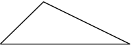
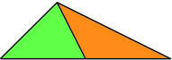
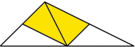
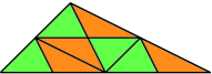
Figure 11. Refinement by newest vertex bisection leads only to finitely many similarity classes of triangles. To see this, we start from a macro element (left), where the bottom edge is the reference edge. Using iterated newest vertex bisection, one observes that only four similarity classes of triangles occur, which are indicated by the coloring. After three levels of bisection (right), no additional similarity class appears.

\psfrag{z}{\tiny$z$}\psfrag{zp}{\tiny$z^{\prime}$}\psfrag{T0}{\tiny${\mathcal{T}}_{0}$}\includegraphics[width=138.76157pt]{figures/counterEx1}

\psfrag{z}{\tiny$z$}\psfrag{zp}{\tiny$z^{\prime}$}\psfrag{T0}{\tiny${\mathcal{T}}_{0}$}\psfrag{T1}{\tiny${\mathcal{T}}_{1}$}\includegraphics[width=138.76157pt]{figures/counterEx2}

\psfrag{z}{\tiny$z$}\psfrag{zp}{\tiny$z^{\prime}$}\psfrag{T0}{\tiny${\mathcal{T}}_{0}$}\psfrag{T1}{\tiny${\mathcal{T}}_{1}$}\psfrag{T2}{\tiny${\mathcal{T}}_{2}$}\includegraphics[width=138.76157pt]{figures/counterEx3}

Figure 12. We consider the sequence of triangulations ${\mathcal{T}}_{0},{\mathcal{T}}_{1},{\mathcal{T}}_{2}$. The initial triangulation ${\mathcal{T}}_{0}$ consists of one triangle. The edges incident to $z\in{\mathcal{N}}_{0}$ have length $\sqrt{5}/2e>0$, whereas the edge opposite to $z$ has length $e>0$. The triangulation ${\mathcal{T}}_{1}$ is obtained from ${\mathcal{T}}_{0}$ by uniform refinement and ${\mathcal{T}}_{2}$ is obtained from ${\mathcal{T}}_{1}=\widehat{\mathcal{T}}_{1}$ by bisecting the longest edge incident to $z$. The shortest edge incident to $z$ in the triangulation ${\mathcal{T}}_{2}$, i.e. $h_{2}(z)$, is spanned by the nodes $z,z^{\prime}$ (red). A simple calculation shows ${\rm level}_{2}(z)=1$. Obviously, $z^{\prime}\notin\widehat{\mathcal{N}}_{1}=\widehat{\mathcal{N}}_{{\rm level}_{2}(z)}$ and the corresponding hat-function $\eta_{z}^{2}$ is not an element of $\widehat{\mathcal{X}}^{1}=\widehat{\mathcal{X}}^{{\rm level}_{2}(z)}$. This shows that the result of Lemma 11 cannot be improved.

4.4. Further auxiliary results

The proof of Proposition 4 requires some additional definitions and technical results. For a given node $z\in\widetilde{\mathcal{N}}_{\ell}$, it may hold $z\in\widetilde{\mathcal{N}}_{\ell+m}$ even with the same level ${\rm level}_{\ell}(z)={\rm level}_{\ell+m}(z)$. We count how often a node $z\in{\mathcal{N}}_{L}$ with a fixed level $k\in{\mathbb{N}}_{0}$ shows up in the sets $\widetilde{\mathcal{N}}_{\ell}$. For $z\in{\mathcal{N}}_{L}$ and $k\in{\mathbb{N}}_{0}$, we therefore define

(53) $$\widetilde{\mathcal{K}}_{k}(z):=\big{\{}\ell\in\{0,1,\dots,L\}\,:\,z\in\widetilde{\mathcal{N}}_{\ell}\quad\text{and}\quad{\rm level}_{\ell}(z)=k\big{\}}.$$

The following lemma from [WC06, Lemma 3.1] proves that the cardinality of these set $\widetilde{\mathcal{K}}_{k}(z)$ is uniformly bounded.

Lemma 8.

For all $z\in{\mathcal{N}}_{L}$ and $k\in{\mathbb{N}}_{0}$, it holds $\#\widetilde{\mathcal{K}}_{k}(z)\leq C_{\ref{constCbound}}$, and the constant $C_{\ref{constCbound}}>0$ depends only on the initial triangulation ${\mathcal{T}}_{0}$, but is independent of $L$, $k$, and $z$.∎

For each $T\in{\mathcal{T}}_{\ell}$, there exists a unique coarse-mesh ancestor $T_{0}\in{\mathcal{T}}_{0}$ with $T\subseteq T_{0}$. For $d=2$, there exists some $k\in{\mathbb{N}}_{0}$ such that $h_{\ell}(T)=2^{-k}h_{0}(T_{0})$, i.e., $T$ is created by $k$ bisections of $T_{0}$ and $k$ thus is the level of $T$. For $d=3$, the successors of $T_{0}$ belong to at most four similarity classes, see Figure 11. Let $\widetilde{T}_{0}\subset T_{0}$ be the unique successor of $T_{0}$ with $T\subseteq\widetilde{T}_{0}$ which is similar to $T$ and has the maximal diameter with respect to its similarity class. Then, there exists $k\in{\mathbb{N}}_{0}$ such that $h_{\ell}(T)=2^{-k}{\rm diam}(\widetilde{T}_{0})$. For both cases ($d=2,3$), we define $r(T)=k$.

For each $z\in{\mathcal{N}}_{\ell}$, we further define the quantity $R_{\ell}(z)$ associated to the patch $\omega_{\ell-1}^{2}(z)$ as

(54) $$R_{\ell}(z):=\min\big{\{}r(T)\,:\,T\in{\mathcal{T}}_{\ell-1},T\subseteq\omega_{\ell-1}^{2}(z)\big{\}}.$$

The proof of the following lemma can be found in [WC06, Proof of Lemma 3.3] for $d=3$. For $d=2$, the proof follows the same lines. Details are left to the reader.

Lemma 9.

(i) For all $z\in{\mathcal{N}}_{\ell}$ holds ${\rm level}_{\ell}(z)\leq R_{\ell}(z)+C_{\ref{constn}}$, and the constant $C_{\ref{constn}}>0$ depends only on the initial triangulation ${\mathcal{T}}_{0}$.
(ii) For all $z\in{\mathcal{N}}_{\ell}$ and $T\in{\mathcal{T}}_{\ell-1}$ with $T\subseteq\omega_{\ell-1}^{2}(z)$, there exists an element $\widehat{T}\in\widehat{\mathcal{T}}_{R_{\ell}(z)}$ such that $T\subseteq\widehat{T}$.∎

Analogously to the patch $\omega_{\ell}^{k}(z)$ from (9), we define the patch $\widehat{\omega}_{m}^{k}(z)$ corresponding to the uniformly refined triangulation $\widehat{\mathcal{T}}_{m}$.

Lemma 10.

There exists $n\in{\mathbb{N}}_{0}$, which depends only on the initial triangulation ${\mathcal{T}}_{0}$, such that for all $z\in{\mathcal{N}}_{\ell}$ holds $\omega_{\ell}(z)\subseteq\omega_{\ell-1}^{2}(z)\subseteq\widehat{\omega}_{{\rm level}_{\ell}(z)}^{n}(z)$.

Proof.

Obviously, $\omega_{\ell}(z)\subseteq\omega_{\ell-1}(z)\subseteq\omega_{\ell-1}^{2}(z)$ by definition of these patches. It remains to prove the second inclusion $\omega_{\ell-1}^{2}(z)\subseteq\widehat{\omega}_{{\rm level}_{\ell}(z)}^{n}(z)$: Lemma 9 states that for $T\in{\mathcal{T}}_{\ell-1}$ with $T\subseteq\omega_{\ell-1}^{2}(z)$, there exists $\widehat{T}\in\widehat{\mathcal{T}}_{R_{\ell}(z)}$ with $T\subseteq\widehat{T}\subseteq\widehat{\omega}_{R_{\ell}(z)}^{2}(z)$. Each element $\widehat{T}\in{\mathcal{T}}_{R_{\ell}(z)}$ with $\widehat{T}\subseteq\widehat{\omega}_{R_{\ell}(z)}^{2}(z)$ is bisected into $2(d-1)C_{\ref{constn}}$ elements $\widehat{T}^{\prime}_{j}\in\widehat{\mathcal{T}}_{R_{\ell}(z)+C_{\ref{constn}}}$ such that

(55) $$\widehat{T}=\bigcup_{j=1}^{2(d-1)C_{\ref{constn}}}\widehat{T}^{\prime}_{j}.$$

In particular, there exists a constant $n\in{\mathbb{N}}$ with $n\leq 4(d-1)C_{\ref{constn}}$ such that $\widehat{T}\subseteq\widehat{\omega}_{R_{\ell}(z)+C_{\ref{constn}}}^{n}(z)$. Lemma 9 states that ${\rm level}_{\ell}(z)\leq R_{\ell}(z)+C_{\ref{constn}}$. Hence, $\widehat{\omega}_{R_{\ell}(z)+C_{\ref{constn}}}^{n}(z)\subseteq\widehat{\omega}_{{\rm level}_{\ell}(z)}^{n}(z)$ by the definition of the patches. ∎

Lemma 11.

For all nodes $z\in{\mathcal{N}}_{\ell}$ holds $\eta_{z}^{\ell}\in\widehat{\mathcal{X}}^{m+1}$ with $m={\rm level}_{\ell}(z)$.

Proof for $d=2$.

We prove that all nodes $z^{\prime}\in{\mathcal{N}}_{\ell}\cap\omega_{\ell}(z)\backslash\{z\}$ satisfy $z^{\prime}\in\widehat{\mathcal{N}}_{m}$. This implies $\eta_{z}^{\ell}\in\widehat{\mathcal{X}}^{m}$. Let $T_{zz^{\prime}}\in{\mathcal{T}}_{\ell}$ denote the element which is spanned by the nodes $z,z^{\prime}$. According to bisection, there exists a coarse mesh-element $T_{0}\in{\mathcal{T}}_{0}$ and $\widehat{n}\in{\mathbb{N}}_{0}$ such that $T_{zz^{\prime}}\in\widehat{\mathcal{X}}^{\widehat{n}}$ with $T_{zz^{\prime}}\subseteq T_{0}$, and $|T_{zz^{\prime}}|=|T_{0}|\,2^{-\widehat{n}}$. The definition of ${\rm level}_{\ell}(z)$ and $h_{\ell}(z)$ yields

$$2^{-m-1}\widehat{h}_{0}<h_{\ell}(z)\leq|T_{zz^{\prime}}|=|T_{0}|\,2^{-\widehat{n}}\leq\widehat{h}_{0}2^{-\widehat{n}}$$

and consequently $m+1>\widehat{n}$. Thus $m\geq\widehat{n}$, and we conclude $z^{\prime}\in\widehat{\mathcal{N}}_{m}\subseteq\widehat{\mathcal{N}}_{m+1}$. ∎

Proof for $d=3$.

Let $E_{zz^{\prime}}$ denote the edge between $z\in{\mathcal{N}}_{\ell}$ and $z^{\prime}\in{\mathcal{N}}_{\ell}\cap\omega_{\ell}(z)\backslash\{z\}$. There exists $\widehat{n}\in{\mathbb{N}}_{0}$ such that $E_{zz^{\prime}}$ is an edge of $\widehat{\mathcal{X}}^{\widehat{n}}$. Furthermore, there exist edges $E_{0},E_{1}$ with $E_{0}\subseteq T_{0}\in{\mathcal{T}}_{0}$, $E_{1}\subseteq T_{1}\in{\mathcal{T}}_{1}$ and $E_{1}$ is a median of the macro element $T_{0}$ such that one of the following cases holds:

• $|E_{zz^{\prime}}|=|E_{0}|\,2^{-\widehat{n}}$ or

• $|E_{zz^{\prime}}|=|E_{1}|\,2^{-\widehat{n}+1}$.

As in the case $d=2$, we obtain $z^{\prime}\in\widehat{\mathcal{N}}_{m}$ for (i) and $z^{\prime}\in\widehat{\mathcal{N}}_{m+1}$ for (ii). Since $\widehat{\mathcal{N}}_{m}\subseteq\widehat{\mathcal{N}}_{m+1}$, this proves $z^{\prime}\in\widehat{\mathcal{N}}_{m+1}$ for all $z^{\prime}\in{\mathcal{N}}_{\ell}\cap\omega_{\ell}(z)$. Hence, $\eta_{z}^{\ell}\in\widehat{\mathcal{X}}^{m+1}$. ∎

In general, the result of the previous Lemma cannot be improved in the sense that there exists a number $k\in{\mathbb{N}}_{0}$ with $k<m+1$ such that $\eta_{z}^{\ell}\in\widehat{\mathcal{X}}^{k}$. See also Figure 12 for an example.

4.5. Proof of Proposition 4, lower bound

In this section, we prove the lower bound in the spectral equivalence estimate (35). The proof relies on the following result which is also known as Lions’ lemma [Lio88, Wid89].

Lemma 12.

Suppose that each $v\in{\mathcal{X}}^{L}$ admits a representation $v=\sum_{\ell=0}^{L}\sum_{z\in\widetilde{\mathcal{N}}_{\ell}}v_{z}^{\ell}$ with $v_{z}^{\ell}\in{\mathcal{X}}_{z}^{\ell}$ and

(56) $$\sum_{\ell=0}^{L}\sum_{z\in\widetilde{\mathcal{N}}_{\ell}}|||v_{z}^{\ell}|||^{2}\leq c^{-1}|||v|||^{2}.$$

Then, $\widetilde{\mathcal{P}}_{\rm AS}^{L}$ is elliptic

(57) $$c\,|||v|||^{2}\leq\langle\langle\widetilde{\mathcal{P}}_{\rm AS}^{L}v\,,\,v\rangle\rangle\quad\text{for all }v\in{\mathcal{X}}^{L},$$

and the minimal eigenvalue of the additive Schwarz operator satisfies $\lambda_{\rm min}(\widetilde{\mathcal{P}}_{\rm AS}^{L})\geq c>0$. ∎

Proof of lower bound in (35).

Let $v\in{\mathcal{X}}^{L}$ and set $J_{-1}:=0$. With the property (49) of the Scott-Zhang projection $J_{\ell}$, we define

(58) $$\widetilde{v}^{\ell}:=(J_{\ell}-J_{\ell-1})v\in\widetilde{\mathcal{X}}^{\ell}\quad\text{for all }0\leq\ell\leq L.$$

The projection property of $J_{L}$ and the telescoping series prove

(59) $$v=J_{L}v=(J_{L}-J_{-1})v=\sum_{\ell=0}^{L}\widetilde{v}^{\ell}.$$

We further decompose $v$ into

(60) $$v=\sum_{\ell=0}^{L}\sum_{z\in\widetilde{\mathcal{N}}_{\ell}}\widetilde{v}^{\ell}(z)\eta_{z}^{\ell}=:\sum_{\ell=0}^{L}\sum_{z\in\widetilde{\mathcal{N}}_{\ell}}v_{z}^{\ell}\quad\text{with }v_{z}^{\ell}\in{\mathcal{X}}_{z}^{\ell}.$$

Let $z\in{\mathcal{N}}_{\ell}$. According to the properties (11) of the hat-functions, standard interpolation techniques yield

(61) $$|||\eta_{z}^{\ell}|||^{2}\simeq\|\eta_{z}^{\ell}\|_{H^{1/2}(\Gamma)}^{2}\leq\|\eta_{z}^{\ell}\|_{L^{2}(\Gamma)}\|\eta_{z}^{\ell}\|_{H^{1}(\Gamma)}\lesssim|\omega_{\ell}(z)|\,h_{\ell}(z)^{-1}\simeq h_{\ell}(z)^{d-2}.$$

This implies

$$|||v_{z}^{\ell}|||^{2}\lesssim h_{\ell}(z)^{d-2}|(J_{\ell}-J_{\ell-1})v(z)|^{2}.$$

We set $\widehat{\Pi}_{m}:=\widehat{\Pi}_{0}$ for $m<0$. Lemma 9 yields that $\widehat{\Pi}_{{\rm level}_{\ell}(z)-C_{\ref{constn}}}v\in\widehat{\mathcal{X}}_{R_{\ell}(z)}$ and that $(\widehat{\Pi}_{{\rm level}_{\ell}(z)-C_{\ref{constn}}}v)|_{T}$ is linear for all $T\in{\mathcal{T}}_{\ell-1}$ with $T\subseteq\omega_{\ell-1}^{2}(z)$. The Scott-Zhang projection preserves linearity on all elements $T\in{\mathcal{T}}_{\ell-1}$ resp. $T\in{\mathcal{T}}_{\ell}$ with $z\in T\subseteq\omega_{\ell-1}^{2}(z)$. This and Lemma 7 yield

$$|(J_{\ell}-J_{\ell-1})v(z)|^{2} =|(J_{\ell}-J_{\ell-1})(v-\widehat{\Pi}_{{\rm level}_{\ell}(z)-C_{\ref{constn}}}v)(z)|^{2}$$

$$\lesssim h_{\ell}(z)^{-(d-1)}\,\|v-\widehat{\Pi}_{{\rm level}_{\ell}(z)-C_{\ref{constn}}}v\|_{L^{2}(\omega_{\ell-1}^{2}(z))}^{2}.$$

Combining the last two estimates, we obtain

$$|||v^{\ell}_{z}|||^{2}\lesssim h_{\ell}(z)^{-1}\,\|v-\widehat{\Pi}_{{\rm level}_{\ell}(z)-C_{\ref{constn}}}v\|_{L^{2}(\omega_{\ell-1}^{2}(z))}^{2}$$

Using the equivalence $h_{\ell}(z)\simeq\widehat{h}_{{\rm level}_{\ell}(z)}$ from Lemma 5, we get

$$\sum_{\ell=0}^{L}\sum_{z\in\widetilde{\mathcal{N}}_{\ell}}|||v_{z}^{\ell}|||^{2} \lesssim\sum_{\ell=0}^{L}\sum_{z\in\widetilde{\mathcal{N}}_{\ell}}h_{\ell}(z)^{-1}\|v-\widehat{\Pi}_{{\rm level}_{\ell}(z)-C_{\ref{constn}}}v\|_{L^{2}(\omega_{\ell-1}^{2}(z))}^{2}$$

$$\simeq\sum_{\ell=0}^{L}\sum_{z\in\widetilde{\mathcal{N}}_{\ell}}\widehat{h}_{{\rm level}_{\ell}(z)}^{-1}\|v-\widehat{\Pi}_{{\rm level}_{\ell}(z)-C_{\ref{constn}}}v\|_{L^{2}(\omega_{\ell-1}^{2}(z))}^{2}$$

$$=\sum_{m=0}^{\infty}\sum_{\ell=0}^{L}\sum_{\begin{subarray}{c}z\in\widetilde{\mathcal{N}}_{\ell}\\ {\rm level}_{\ell}(z)=m\end{subarray}}\widehat{h}_{m}^{-1}\|v-\widehat{\Pi}_{m-C_{\ref{constn}}}v\|_{L^{2}(\omega_{\ell-1}^{2}(z))}^{2}.$$

With Lemma 10 and the definition (53) of $\widetilde{\mathcal{K}}_{m}(z)$, we see

$$\sum_{m=0}^{\infty}\sum_{\ell=0}^{L}\!\!\sum_{\begin{subarray}{c}z\in\widetilde{\mathcal{N}}_{\ell}\\ {\rm level}_{\ell}(z)=m\end{subarray}}\!\!\widehat{h}_{m}^{-1}\|v-\widehat{\Pi}_{m-C_{\ref{constn}}}v\|_{L^{2}(\omega_{\ell-1}^{2}(z))}^{2} \lesssim\sum_{m=0}^{\infty}\sum_{\ell=0}^{L}\!\!\sum_{\begin{subarray}{c}z\in\widetilde{\mathcal{N}}_{\ell}\\ {\rm level}_{\ell}(z)=m\end{subarray}}\!\!\widehat{h}_{m}^{-1}\|v-\widehat{\Pi}_{m-C_{\ref{constn}}}v\|_{L^{2}(\widehat{\omega}_{m}^{n}(z))}^{2}$$

$$=\sum_{m=0}^{\infty}\sum_{z\in{\mathcal{N}}_{L}}\sum_{\ell\in\widetilde{\mathcal{K}}_{m}(z)}\widehat{h}_{m}^{-1}\|v-\widehat{\Pi}_{m-C_{\ref{constn}}}v\|_{L^{2}(\widehat{\omega}_{m}^{n}(z))}^{2}.$$

For $z\in{\mathcal{N}}_{\ell}$ with ${\rm level}_{\ell}(z)=m$, Lemma 5 states $z\in\widehat{\mathcal{N}}_{m}$. This and $\#\widetilde{\mathcal{K}}_{m}(z)\leq C_{\ref{constCbound}}$ from Lemma 8 give

$$\sum_{m=0}^{\infty}\sum_{z\in{\mathcal{N}}_{L}}\sum_{\ell\in\widetilde{\mathcal{K}}_{m}(z)}\widehat{h}_{m}^{-1}\|v-\widehat{\Pi}_{m-C_{\ref{constn}}}v\|_{L^{2}(\widehat{\omega}_{m}^{n}(z))}^{2} =\sum_{m=0}^{\infty}\sum_{z\in{\mathcal{N}}_{L}\cap\widehat{\mathcal{N}}_{m}}\sum_{\ell\in\widetilde{\mathcal{K}}_{m}(z)}\widehat{h}_{m}^{-1}\|v-\widehat{\Pi}_{m-C_{\ref{constn}}}v\|_{L^{2}(\widehat{\omega}_{m}^{n}(z))}^{2}$$

$$\lesssim\sum_{m=0}^{\infty}\sum_{z\in{\mathcal{N}}_{L}\cap\widehat{\mathcal{N}}_{m}}\widehat{h}_{m}^{-1}\|v-\widehat{\Pi}_{m-C_{\ref{constn}}}v\|_{L^{2}(\widehat{\omega}_{m}^{n}(z))}^{2}$$

$$\leq\sum_{m=0}^{\infty}\sum_{z\in\widehat{\mathcal{N}}_{m}}\widehat{h}_{m}^{-1}\|v-\widehat{\Pi}_{m-C_{\ref{constn}}}v\|_{L^{2}(\widehat{\omega}_{m}^{n}(z))}^{2}.$$

Uniform $\gamma$-shape regularity of $\widehat{\mathcal{T}}_{m}$ and the definition $\widehat{\Pi}_{m}=\widehat{\Pi}_{0}$ for $m<0$ yield

$$\sum_{m=0}^{\infty}\sum_{z\in\widehat{\mathcal{N}}_{m}}\widehat{h}_{m}^{-1}\|v-\widehat{\Pi}_{m-C_{\ref{constn}}}v\|_{L^{2}(\widehat{\omega}_{m}^{n}(z))}^{2} \lesssim\sum_{m=0}^{\infty}\widehat{h}_{m}^{-1}\|v-\widehat{\Pi}_{m-C_{\ref{constn}}}v\|_{L^{2}(\Gamma)}^{2}\lesssim\sum_{m=0}^{\infty}\widehat{h}_{m}^{-1}\|v-\widehat{\Pi}_{m}v\|_{L^{2}(\Gamma)}^{2}$$

We combine the last four estimates with Lemma 6 and norm equivalence on $H^{1/2}(\Gamma)$ to see

$$\sum_{\ell=0}^{L}\sum_{z\in\widetilde{\mathcal{N}}_{\ell}}|||\widetilde{v}_{z}^{\ell}|||^{2}\lesssim\sum_{m=0}^{\infty}\widehat{h}_{m}^{-1}\|v-\widehat{\Pi}_{m}v\|_{L^{2}(\Gamma)}^{2}\lesssim\|v\|_{H^{1/2}(\Gamma)}^{2}\simeq|||v|||^{2}.$$

This and Lemma 12 then conclude the proof of the lower bound in (35). ∎

4.6. Proof of Proposition 4, upper bound

In this section, we prove the upper bound in the spectral equivalence estimate (35).

Let $M:=\max_{z\in{\mathcal{N}}_{L}}{\rm level}_{L}(z)$ denote the maximal level of all nodes $z\in{\mathcal{N}}_{L}$ and note that Lemma 5 yields ${\mathcal{N}}_{L}\subseteq\widehat{\mathcal{N}}_{M}$ and hence ${\mathcal{X}}^{L}\subseteq\widehat{\mathcal{X}}^{M}$. We rewrite the additive Schwarz operator $\widetilde{\mathcal{P}}_{\rm AS}^{L}$ as

(62) $$\widetilde{\mathcal{P}}_{\rm AS}^{L}=\sum_{\ell=0}^{L}\sum_{z\in\widetilde{\mathcal{N}}_{\ell}}\mathcal{P}_{z}^{\ell}=\sum_{m=0}^{M}\widetilde{\mathcal{Q}}_{m}^{L}\quad\text{with}\quad\widetilde{\mathcal{Q}}_{m}^{L}:=\sum_{\ell=0}^{L}\sum_{\begin{subarray}{c}z\in\widetilde{\mathcal{N}}_{\ell}\\ {\rm level}_{\ell}(z)=m\end{subarray}}\mathcal{P}_{z}^{\ell}.$$

There holds the following strengthened Cauchy-Schwarz inequality.

Lemma 13.

For all $0\leq m\leq M$, $k\leq m+1$

(63) $$0\leq\langle\langle\widetilde{\mathcal{Q}}^{L}_{m}\widehat{v}^{k}\,,\,\widehat{v}^{k}\rangle\rangle\leq C_{\ref{constcsu}}2^{-(m+1-k)}|||\widehat{v}^{k}|||^{2}\quad\text{for all }\widehat{v}^{k}\in\widehat{\mathcal{X}}^{k}.$$

The constant $C_{\ref{constcsu}}>0$ depends only on $\Gamma$ and the initial triangulation ${\mathcal{T}}_{0}$.

Proof.

By definition of $\widetilde{\mathcal{Q}}_{m}^{L}$, it holds

(64) $$\langle\langle\widetilde{\mathcal{Q}}_{m}^{L}\widehat{v}^{k}\,,\,\widehat{v}^{k}\rangle\rangle =\sum_{\ell=0}^{L}\sum_{\begin{subarray}{c}z\in\widetilde{\mathcal{N}}_{\ell}\\ {\rm level}_{\ell}(z)=m\end{subarray}}\langle\langle\mathcal{P}_{z}^{\ell}\widehat{v}^{k}\,,\,\widehat{v}^{k}\rangle\rangle=\sum_{\ell=0}^{L}\sum_{\begin{subarray}{c}z\in\widetilde{\mathcal{N}}_{\ell}\\ {\rm level}_{\ell}(z)=m\end{subarray}}|||\mathcal{P}_{z}^{\ell}\widehat{v}^{k}|||^{2}\geq 0.$$

Let $z\in\widetilde{\mathcal{N}}_{\ell}$ with ${\rm level}_{\ell}(z)=m$. Lemma 5 states $h_{\ell}(z)\simeq\widehat{h}_{m}$ and $z\in\widetilde{\mathcal{N}}_{\ell}\cap\widehat{\mathcal{N}}_{m}$. From the representation (27) of $\mathcal{P}_{z}^{\ell}$, we get

(65) $$\langle\langle\mathcal{P}_{z}^{\ell}\widehat{v}^{k}\,,\,\widehat{v}^{k}\rangle\rangle=\frac{\langle\langle\widehat{v}^{k}\,,\,\eta_{z}^{\ell}\rangle\rangle^{2}}{|||\eta_{z}^{\ell}|||^{2}}\lesssim\frac{\langle\mathcal{W}\widehat{v}^{k}\,,\,\eta_{z}^{\ell}\rangle_{\Gamma}^{2}+\langle\widehat{v}^{k}\,,\,1\rangle_{\Gamma}^{2}\langle\eta_{z}^{\ell}\,,\,1\rangle_{\Gamma}^{2}}{|||\eta_{z}^{\ell}|||^{2}}.$$

According to, e.g., [AMT99, Theorem 4.8], it holds $h_{\ell}(z)^{s}\,\|\eta_{z}^{\ell}\|_{H^{s}(\Gamma)}\simeq\|\eta_{z}^{\ell}\|_{L^{2}(\Gamma)}$, where the hidden constants depends on $\Gamma$, $0\leq s\leq 1$, and $\gamma$-shape regularity of ${\mathcal{T}}_{\ell}$. With $h_{\ell}(z)\,|||\eta_{z}^{\ell}|||^{2}\simeq h_{\ell}(z)\,\|\eta_{z}^{\ell}\|_{H^{1/2}(\Gamma)}^{2}\simeq\|\eta_{z}^{\ell}\|_{L^{2}(\Gamma)}^{2}$, the Cauchy-Schwarz inequality thus gives

$$\frac{\langle\mathcal{W}\widehat{v}^{k}\,,\,\eta_{z}^{\ell}\rangle_{\Gamma}^{2}}{|||\eta_{z}^{\ell}|||^{2}}\lesssim h_{\ell}(z)\|\mathcal{W}\widehat{v}^{k}\|_{L^{2}(\omega_{\ell}(z))}^{2}\lesssim\frac{\widehat{h}_{m}}{\widehat{h}_{k}}\,\|\widehat{h}_{k}^{1/2}\mathcal{W}\widehat{v}^{k}\|_{L^{2}(\omega_{\ell}(z))}^{2}\lesssim 2^{-(m+1-k)}\,\|\widehat{h}_{k}^{1/2}\mathcal{W}\widehat{v}^{k}\|_{L^{2}(\omega_{\ell}(z))}^{2}.$$

For the stabilization term, the same arguments together with $\langle\eta_{z}^{\ell}\,,\,1\rangle_{\Gamma}\leq\|\eta_{z}^{\ell}\|_{L^{2}(\Gamma)}|\omega_{\ell}(z)|^{1/2}$ yield

$$\frac{\langle\widehat{v}^{k}\,,\,1\rangle_{\Gamma}^{2}\langle\eta_{z}^{\ell}\,,\,1\rangle_{\Gamma}^{2}}{|||\eta_{z}^{\ell}|||^{2}} \lesssim h_{\ell}(z)|\omega_{\ell}(z)|\|\widehat{v}^{k}\|_{H^{1/2}(\Gamma)}^{2}\lesssim 2^{-(m+1-k)}\,|\omega_{\ell}(z)|\|\widehat{v}^{k}\|_{H^{1/2}(\Gamma)}^{2},$$

where the last estimate follows from $h_{\ell}(z)\simeq\widehat{h}_{m}\lesssim\widehat{h}_{m}/\widehat{h}_{k}=2\cdot 2^{-(m+1-k)}$. Combining these three estimates, we obtain

$$\langle\langle\mathcal{P}_{z}^{\ell}\widehat{v}^{k}\,,\,\widehat{v}^{k}\rangle\rangle\lesssim 2^{-(m+1-k)}\,\big{(}\|\widehat{h}_{k}^{1/2}\mathcal{W}\widehat{v}^{k}\|_{L^{2}(\omega_{\ell}(z))}^{2}+|\omega_{\ell}(z)|\|\widehat{v}^{k}\|_{H^{1/2}(\Gamma)}^{2}\big{)}$$

By Lemma 10, we have $\omega_{\ell}(z)\subseteq\widehat{\omega}_{m}^{n}(z)$. The representation of $\widetilde{\mathcal{Q}}_{m}^{L}$ from (64) thus gives

$$\langle\langle\widetilde{\mathcal{Q}}_{m}^{L}\widehat{v}^{k}\,,\,\widehat{v}^{k}\rangle\rangle \lesssim 2^{-(m+1-k)}\sum_{\ell=0}^{L}\sum_{\begin{subarray}{c}z\in\widetilde{\mathcal{N}}_{\ell}\\ {\rm level}_{\ell}(z)=m\end{subarray}}(\|\widehat{h}_{k}^{1/2}\mathcal{W}\widehat{v}^{k}\|_{L^{2}(\widehat{\omega}_{m}^{n}(z))}^{2}+|\widehat{\omega}_{m}^{n}(z)|\|\widehat{v}^{k}\|_{H^{1/2}(\Gamma)}^{2}).$$

By definition (53) of $\widetilde{\mathcal{K}}_{m}(z)$ and Lemma 8, the double sum can be rewritten and further estimated by

(66) $$\begin{split}\sum_{\ell=0}^{L}\sum_{\begin{subarray}{c}z\in\widetilde{\mathcal{N}}_{\ell}\\ {\rm level}_{\ell}(z)=m\end{subarray}}&\big{(}\|\widehat{h}_{k}^{1/2}\mathcal{W}\widehat{v}^{k}\|_{L^{2}(\widehat{\omega}_{m}^{n}(z))}^{2}+|\widehat{\omega}_{m}^{n}(z)|\|\widehat{v}^{k}\|_{H^{1/2}(\Gamma)}^{2}\big{)}\\ &=\sum_{z\in\widehat{\mathcal{N}}_{m}\cap{\mathcal{N}}_{L}}\sum_{\ell\in\widetilde{\mathcal{K}}_{m}(z)}\big{(}\|\widehat{h}_{k}^{1/2}\mathcal{W}\widehat{v}^{k}\|_{L^{2}(\widehat{\omega}_{m}^{n}(z))}^{2}+|\widehat{\omega}_{m}^{n}(z)|\|\widehat{v}^{k}\|_{H^{1/2}(\Gamma)}^{2}\big{)}\\ &\lesssim\sum_{z\in\widehat{\mathcal{N}}_{m}\cap{\mathcal{N}}_{L}}\big{(}\|\widehat{h}_{k}^{1/2}\mathcal{W}\widehat{v}^{k}\|_{L^{2}(\widehat{\omega}_{m}^{n}(z))}^{2}+|\widehat{\omega}_{m}^{n}(z)|\|\widehat{v}^{k}\|_{H^{1/2}(\Gamma)}^{2}\big{)}\\ &\leq\sum_{z\in\widehat{\mathcal{N}}_{m}}\big{(}\|\widehat{h}_{k}^{1/2}\mathcal{W}\widehat{v}^{k}\|_{L^{2}(\widehat{\omega}_{m}^{n}(z))}^{2}+|\widehat{\omega}_{m}^{n}(z)|\|\widehat{v}^{k}\|_{H^{1/2}(\Gamma)}^{2}\big{)}\end{split}$$

By $\gamma$-shape regularity of $\widehat{\mathcal{T}}_{m}$, it holds

$$\sum_{z\in\widehat{\mathcal{N}}_{m}}\big{(}\|\widehat{h}_{k}^{1/2}\mathcal{W}\widehat{v}^{k}\|_{L^{2}(\widehat{\omega}_{m}^{n}(z))}^{2}+|\widehat{\omega}_{m}^{n}(z)|\|\widehat{v}^{k}\|_{H^{1/2}(\Gamma)}^{2}\big{)} \lesssim\|\widehat{h}_{k}^{1/2}\mathcal{W}\widehat{v}^{k}\|_{L^{2}(\Gamma)}^{2}+\|\widehat{v}^{k}\|_{H^{1/2}(\Gamma)}^{2}.$$

Recall stability $\mathcal{W}:H^{1}(\Gamma)\to L^{2}(\Gamma)$. Together with an inverse estimate between $H^{1}(\Gamma)$ and $H^{1/2}(\Gamma)$ for piecewise polynomials, see e.g. [AFF⁺13b, Proposition 5], we obtain

(67) $$\|\widehat{h}_{k}^{1/2}\mathcal{W}\widehat{v}^{k}\|_{L^{2}(\Gamma)}^{2}=\widehat{h}_{k}\|\mathcal{W}\widehat{v}^{k}\|_{L^{2}(\Gamma)}^{2}\lesssim\widehat{h}_{k}\|\widehat{v}^{k}\|_{H^{1}(\Gamma)}^{2}\lesssim\|\widehat{v}^{k}\|_{H^{1/2}(\Gamma)}^{2}.$$

We note that the latter estimate does not only hold for uniform triangulations $\widehat{\mathcal{T}}_{k}$, but also for shape-regular triangulations and higher-order polynomials [AFF⁺12, Corollary 2]. Combining the last four estimates with norm equivalence $\|\widehat{v}^{k}\|_{H^{1/2}(\Gamma)}\simeq|||\widehat{v}^{k}|||$, we conclude the proof. ∎

The rest of the proof follows along the lines of the proof of [TS96, Lemma 2.8] and is given for completeness. We note that Lemma 13 implies, in particular, that $\langle\langle\widetilde{\mathcal{Q}}_{m}^{L}v\,,\,w\rangle\rangle$ defines a positive semi-definite and symmetric bilinear form on $\widehat{\mathcal{X}}^{k}$ for $k\leq m+1$ and hence satisfies a Cauchy-Schwarz inequality.

Proof of upper bound in (35).

Let $\widehat{\mathcal{G}}_{m}:H^{1/2}(\Gamma)\to\widehat{\mathcal{X}}^{m}$ denote the Galerkin projection onto $\widehat{\mathcal{X}}^{m}$ with respect to the scalar product $\langle\langle\cdot\,,\,\cdot\rangle\rangle$, i.e.,

(68) $$\langle\langle\widehat{\mathcal{G}}_{m}v\,,\,\widehat{w}^{m}\rangle\rangle=\langle\langle v\,,\,\widehat{w}^{m}\rangle\rangle\quad\text{for all }\widehat{w}^{m}\in\widehat{\mathcal{X}}^{m}.$$

Note that $\widehat{\mathcal{G}}_{m}$ is the orthogonal projection onto $\widehat{\mathcal{X}}^{m}$ with respect to the energy norm $|||\cdot|||$. We set $\widehat{\mathcal{G}}_{-1}:=0$. For any $v\in{\mathcal{X}}^{L}\subseteq\widehat{\mathcal{X}}^{M}$, it holds

(69) $$\widehat{\mathcal{G}}_{m}v=\sum_{k=0}^{m}(\widehat{\mathcal{G}}_{k}-\widehat{\mathcal{G}}_{k-1})v\quad\text{as well as}\quad\widehat{\mathcal{G}}_{M}v=v=\widehat{\mathcal{G}}_{M+1}v.$$

Lemma 11 yields $\widetilde{\mathcal{Q}}_{m}^{L}v\in\widehat{\mathcal{X}}^{m+1}$. The symmetry of the orthogonal projection $\widehat{\mathcal{G}}_{m}$ hence shows

$$\langle\langle\widetilde{\mathcal{Q}}_{m}^{L}v\,,\,v\rangle\rangle=\langle\langle\widetilde{\mathcal{Q}}_{m}^{L}v\,,\,\widehat{\mathcal{G}}_{m+1}v\rangle\rangle =\sum_{k=0}^{m+1}\langle\langle\mathcal{P}_{m}^{L}v\,,\,(\widehat{\mathcal{G}}_{k}-\widehat{\mathcal{G}}_{k-1})v\rangle\rangle$$

$$\leq\sum_{k=0}^{m+1}\langle\langle\widetilde{\mathcal{Q}}_{m}^{L}v\,,\,v\rangle\rangle^{1/2}\langle\langle\widetilde{\mathcal{Q}}_{m}^{L}(\widehat{\mathcal{G}}_{k}-\widehat{\mathcal{G}}_{k-1})v\,,\,(\widehat{\mathcal{G}}_{k}-\widehat{\mathcal{G}}_{k-1})v\rangle\rangle^{1/2},$$

where we have used the Cauchy-Schwarz inequality for $\langle\langle\widetilde{\mathcal{Q}}_{m}^{L}v\,,\,w\rangle\rangle$ with $w=(\widehat{\mathcal{G}}_{k}-\widehat{\mathcal{G}}_{k-1})v\in\widehat{\mathcal{X}}^{k}$. For the second scalar product, we apply Lemma 13 and obtain

$$\langle\langle\widetilde{\mathcal{Q}}_{m}^{L}(\widehat{\mathcal{G}}_{k}-\widehat{\mathcal{G}}_{k-1})v\,,\,(\widehat{\mathcal{G}}_{k}-\widehat{\mathcal{G}}_{k-1})v\rangle\rangle\lesssim 2^{-(m+1-k)}\,|||(\widehat{\mathcal{G}}_{k}-\widehat{\mathcal{G}}_{k-1})v|||^{2}=2^{-(m+1-k)}\langle\langle(\widehat{\mathcal{G}}_{k}-\widehat{\mathcal{G}}_{k-1})v\,,\,v\rangle\rangle$$

With the representation (62) of $\widetilde{\mathcal{P}}_{\rm AS}^{L}$ and the Young inequality, we infer

$$\langle\langle\widetilde{\mathcal{P}}_{\rm AS}^{L}v\,,\,v\rangle\rangle =\sum_{m=0}^{M}\langle\langle\widetilde{\mathcal{Q}}_{m}^{L}v\,,\,v\rangle\rangle$$

$$\leq\frac{\delta}{2}\sum_{m=0}^{M}\sum_{k=0}^{m+1}2^{-(m+1-k)/2}\langle\langle\widetilde{\mathcal{Q}}_{m}^{L}v\,,\,v\rangle\rangle+\frac{\delta^{-1}}{2}\sum_{m=0}^{M}\sum_{k=0}^{m+1}2^{-(m+1-k)/2}\langle\langle\widehat{\mathcal{G}}_{k}-\widehat{\mathcal{G}}_{k-1})v\,,\,v\rangle\rangle,$$

for all $\delta>0$. There holds $\sum_{k=0}^{m+1}2^{-(m+1-k)/2}\leq\sum_{k=0}^{\infty}2^{-k/2}=:K<\infty$. Changing the summation indices in the second sum, we see

$$\langle\langle\widetilde{\mathcal{P}}_{\rm AS}^{L}v\,,\,v\rangle\rangle \leq K\frac{\delta}{2}\,\sum_{m=0}^{M}\langle\langle\widetilde{\mathcal{Q}}_{m}^{L}v\,,\,v\rangle\rangle+\frac{\delta^{-1}}{2}\,\sum_{k=0}^{M+1}\sum_{m=k-1}^{M}2^{-(m+1-k)/2}\langle\langle(\widehat{\mathcal{G}}_{k}-\widehat{\mathcal{G}}_{k-1})v\,,\,v\rangle\rangle$$

$$\leq K\frac{\delta}{2}\,\sum_{m=0}^{M}\langle\langle\widetilde{\mathcal{Q}}_{m}^{L}v\,,\,v\rangle\rangle+K\frac{\delta^{-1}}{2}\,\sum_{k=0}^{M+1}\langle\langle(\widehat{\mathcal{G}}_{k}-\widehat{\mathcal{G}}_{k-1})v\,,\,v\rangle\rangle$$

$$=K\frac{\delta}{2}\langle\langle\widetilde{\mathcal{P}}_{\rm AS}^{L}v\,,\,v\rangle\rangle+K\frac{\delta^{-1}}{2}\langle\langle v\,,\,v\rangle\rangle,$$

where the final equality follows from the telescoping series and $\widehat{\mathcal{G}}_{M+1}v=v$. Choosing $\delta>0$ sufficiently small and absorbing the first-term on the right-hand side on the left, we conclude the upper bound in (35). ∎

5. Proof of Theorem 2

Clearly, the abstract analytical setting for additive Schwarz operators from Section 4.1 also applies for the operator

(70) $$\mathcal{P}_{\rm AS}^{L}=\sum_{\ell=0}^{L}\sum_{z\in{\mathcal{N}}_{\ell}}\mathcal{P}_{z}^{\ell}$$

associated to the preconditioner defined in Section 2.6. We stress that the properties of $(\mathbf{B}^{L})^{-1}$ and $\mathbf{P}_{\rm AS}$ follow in the same way as for Theorem 1. It thus remains to provide a lower and upper bound for the operator $\mathcal{P}_{\rm AS}^{L}$ in analogy to Proposition 4 for $\widetilde{\mathcal{P}}_{\rm AS}^{L}$.

Proposition 14.

The operator $\mathcal{P}_{\rm AS}^{L}$ satisfies

(71) $$c\,|||v|||^{2}\leq\langle\langle\mathcal{P}_{\rm AS}^{L}v\,,\,v\rangle\rangle\leq C(L+1)\,|||v|||^{2}\quad\text{for all }v\in{\mathcal{X}}^{L}.$$

The constants $c,C>0$ depend only on $\Gamma$ and the initial triangulation ${\mathcal{T}}_{0}$.

In principle, the proof follows the same lines as in Section 4.5–4.6. We sketch the most important modifications only. Details are left to the reader.

5.1. Proof of lower bound in (71)

By virtue of Lemma 12, we need to construct a decomposition $v=\sum_{\ell=0}^{L}\sum_{z\in{\mathcal{N}}_{\ell}}v_{z}^{\ell}$ with $v_{z}^{\ell}\in{\mathcal{X}}_{z}^{\ell}$ and $\sum_{\ell=0}^{L}\sum_{z\in{\mathcal{N}}_{\ell}}|||v_{z}^{\ell}|||^{2}\leq c^{-1}|||v|||^{2}$, for all $v\in{\mathcal{X}}^{L}$. Since $\widetilde{\mathcal{N}}_{\ell}\subseteq{\mathcal{N}}_{\ell}$, we may rely on the same decomposition as in Section 4.5. This concludes the proof with the same constant $c>0$ for Proposition 4 and Proposition 14.

5.2. Proof of upper bound in (71)

For the proof of the upper bound in (71), we define the set

(72) $${\mathcal{K}}_{k}(z):=\big{\{}\ell\in\{0,1,\dots,L\}\,:\,z\in{\mathcal{N}}_{\ell}\quad\text{and}\quad{\rm level}_{\ell}(z)=k\big{\}}.$$

Lemma 15.

For all $z\in{\mathcal{N}}_{L}$ and $k\in{\mathbb{N}}_{0}$ there holds

$$\#{\mathcal{K}}_{k}(z)\leq L+1.$$

Proof.

Obviously, there are at most $L+1$ indices in the set ${\mathcal{K}}_{k}(z)$. ∎

We proceed as in Section 4.6 and provide a similar result as in Lemma 13, where, however, Lemma 15 plays an important role in the proof. To that end, we define the operator ${\mathcal{Q}}_{m}^{L}:{\mathcal{X}}^{L}\to\widehat{\mathcal{X}}^{m+1}$ by

$${\mathcal{Q}}_{m}^{L}:=\sum_{\ell=0}^{L}\sum_{\begin{subarray}{c}z\in{\mathcal{N}}_{\ell}\\ {\rm level}_{\ell}(z)=m\end{subarray}}\mathcal{P}_{z}^{\ell},$$

and stress that

$$\mathcal{P}_{\rm AS}^{L}=\sum_{m=0}^{M}{\mathcal{Q}}_{m}^{L}.$$

Lemma 16.

For all $0\leq m\leq M$, $k\leq m+1$

(73) $$0\leq\langle\langle{\mathcal{Q}}^{L}_{m}\widehat{v}^{k}\,,\,\widehat{v}^{k}\rangle\rangle\leq C_{\ref{constcsugmld}}\,(L+1)\,2^{-(m+1-k)}|||\widehat{v}^{k}|||^{2}\quad\text{for all }\widehat{v}^{k}\in\widehat{\mathcal{X}}^{k}.$$

The constant $C_{\ref{constcsugmld}}>0$ depends only on $\Gamma$ and the initial triangulation ${\mathcal{T}}_{0}$.

Proof.

The proof follows the same lines as the proof of Lemma 13. The important modifications consist in replacing $\widetilde{\mathcal{N}}_{\ell}$ by ${\mathcal{N}}_{\ell}$, $\widetilde{\mathcal{K}}_{m}(z)$ by ${\mathcal{K}}_{m}(z)$, and $\widetilde{\mathcal{Q}}_{m}^{L}$ by ${\mathcal{Q}}_{m}^{L}$. However, in estimate (66) a bound for the cardinality of the set $\widetilde{\mathcal{K}}_{m}(z)$ enters. Clearly, we have to replace this bound by the bound for $\#{\mathcal{K}}_{m}(z)$ from Lemma 15. Therefore, the factor $L+1$ comes into estimate (73). ∎

The rest of the proof is a simple adaptation of Section 4.6, taking care of the additional factor $L+1$. It is therefore left to the reader.

6. Extension to screen problems

6.1. Continuous setting

Let $\Gamma\subsetneqq\partial\Omega$ denote an open screen. By $\widetilde{H}^{1/2}(\Gamma)$, we denote the space of $H^{1/2}(\partial\Omega)$ functions which vanish outside of $\Gamma$. It is known [Ste87] that the hypersingular integral operator $\mathcal{W}:\widetilde{H}^{1/2}(\Gamma)\to H^{-1/2}(\Gamma)$ from (1) is a linear, bounded, symmetric, and elliptic operator. The definition

(74) $$\langle\langle v\,,\,w\rangle\rangle:=\langle\mathcal{W}u\,,\,w\rangle_{\Gamma}\quad\text{for all }v,w\in\widetilde{H}^{1/2}(\Gamma)$$

provides a scalar product on $\widetilde{H}^{1/2}(\Gamma)$, and the induced norm $|||v|||^{2}:=\langle\langle v\,,\,v\rangle\rangle$ is an equivalent norm on $\widetilde{H}^{1/2}(\Gamma)$. Instead of (4), we consider the variational formulation of the hypersingular integral equation (1)

(75) $$\langle\langle u\,,\,v\rangle\rangle=\langle f\,,\,v\rangle_{\Gamma}\quad\text{for all }v\in\widetilde{H}^{1/2}(\Gamma)$$

with right-hand side $f\in H^{-1/2}(\Gamma)$. The lemma of Lax-Milgram proves that this formulation admits a unique solution $u\in\widetilde{H}^{1/2}(\Gamma)$.

6.2. Notations

We use the same notations as in Section 2.2–2.4. The discrete space ${\mathcal{X}}^{\ell}$ from (7) is replaced by the definition

(76) $${\mathcal{X}}^{\ell}:=\SS_{0}^{1}({\mathcal{T}}_{\ell}):=\SS^{1}({\mathcal{T}}_{\ell})\cap\widetilde{H}^{1/2}(\Gamma),$$

i.e. the space of piecewise linear and globally continuous functions, which vanish outside the open boundary part $\Gamma$. Moreover, the set ${\mathcal{N}}_{\ell}$ now does not consist of all nodes of the triangulation ${\mathcal{T}}_{\ell}$, but only of the nodes which lie inside $\Gamma$, i.e.

(77) $${\mathcal{N}}_{\ell}:=\{z\text{ is a node of }{\mathcal{T}}_{\ell}\text{ which lies inside }\Gamma\text{ but not on the relative boundary }\partial\Gamma.\}$$

Clearly, $\#{\mathcal{N}}_{\ell}=\dim(\SS_{0}^{1}(\Gamma))$. Also note that the definition (14) of the set $\widetilde{\mathcal{N}}_{\ell}$ involves the set ${\mathcal{N}}_{\ell}$.

The uniformly refined spaces $\widehat{\mathcal{X}}^{m}$ are defined accordingly.

6.3. Multilevel diagonal preconditioner

We stick with the settings and notations as in Section 2.5–2.6.

Theorem 17.

Theorem 1 and Theorem 2 hold for screen problems.

Proof.

First, we extend Theorem 1 to problems on open boundaries. Note that the abstract analysis of additive Schwarz operators from Section 4 holds also for $\Gamma\subsetneqq\partial\Omega$. In particular, we only need to prove the lower and upper bound from Proposition 4.

We stress that Lemma 5–11 hold accordingly if $H^{1/2}$ is replaced by $\widetilde{H}^{1/2}$:

• Lemma 5, Lemma 8–11 hold for this problem, since they are only related to the triangulations and the mesh-refinement procedure.

• Lemma 6 remains valid if $H^{1/2}$ is replaced by $\widetilde{H}^{1/2}$, since the equivalence (42) also holds for $\Gamma\subsetneqq\partial\Omega$ and $H^{1/2}$ replaced by $\widetilde{H}^{1/2}$, see [AM03, Theorem 5].

• Lemma 7 involves a variant of the Scott-Zhang operator, which has to be constructed appropriately, see Section 4.3 and the references therein. To this end, one may proceed as in [AFF⁺13b] with the restriction on the choice of the elements $T_{z}^{\ell}$ required here, so that Lemma 7 remains valid.

Altogether, the proof of the lower bound follows the same lines as in Section 4.5. Clearly, the Sobolev space $H^{1/2}(\Gamma)$ has to be replaced by $\widetilde{H}^{1/2}(\Gamma)$. Note that our re-definition (77) of ${\mathcal{N}}_{\ell}$ for $\Gamma\subsetneqq\partial\Omega$ ensures that the hat-function $\eta_{z}^{\ell}$ vanishes outside of $\Gamma$ for all $z\in{\mathcal{N}}_{\ell}$. Thus, $\omega_{\ell}(z)={\rm supp}(\eta_{z}^{\ell})\subseteq\overline{\Gamma}$ and

(78) $$\|\eta_{z}^{\ell}\|_{\widetilde{H}^{1/2}(\Gamma)}=\|\eta_{z}^{\ell}\|_{H^{1/2}(\partial\Omega)}.$$

Therefore, estimate (61) holds, since

(79) $$|||\eta_{z}^{\ell}|||^{2}\simeq\|\eta_{z}^{\ell}\|_{\widetilde{H}^{1/2}(\Gamma)}^{2}=\|\eta_{z}^{\ell}\|_{H^{1/2}(\partial\Omega)}^{2}\leq\|\eta_{z}^{\ell}\|_{L^{2}(\partial\Omega)}\|\eta_{z}^{\ell}\|_{H^{1}(\partial\Omega)}\lesssim h_{\ell}(z)^{d-2}.$$

The rest of the proof holds verbatim with the notational adaptations mentioned above.

Finally, we stress that for the proof of the upper bound in Proposition 4, one has to verify Lemma 13 only. Due to (78) and [AMT99, Theorem 4.8], we get

$$h_{\ell}(z)^{1/2}\|\eta_{z}^{\ell}\|_{\widetilde{H}^{1/2}(\Gamma)}=h_{\ell}(z)^{1/2}\|\eta_{z}^{\ell}\|_{H^{1/2}(\partial\Omega)}\simeq\|\eta_{z}^{\ell}\|_{L^{2}(\partial\Omega)}=\|\eta_{z}^{\ell}\|_{L^{2}(\Gamma)}.$$

The inverse-type estimate (67) for the hypersingular integral operator $\mathcal{W}$ still hold true for open boundary parts $\Gamma$ and $H^{1/2}(\Gamma)$ replaced by $\widetilde{H}^{1/2}(\Gamma)$. Then, the same proof as for Lemma 13 can be used, if the stabilization terms from equation (65) and the following equations are omitted.

The extension of Theorem 2 to problems on open boundaries can be obtained by the modifications from above and Section 5. Details are left to the reader. ∎

References

- [AEF+11] Markus Aurada, Michael Ebner, Michael Feischl, Samuel Ferraz-Leite, Thomas Führer, Petra Goldenits, Michael Karkulik, Markus Mayr, and Dirk Praetorius. A Matlab implementation of adaptive 2D-BEM. ASC Report, 24/2011, Vienna University of Technology, 2011.
- [AFF+12] Markus Aurada, Michael Feischl, Thomas Führer, Michael Karkulik, Jens Markus Melenk, and Dirk Praetorius. Inverse estimates for elliptic boundary integral operators and their application to the adaptive coupling of FEM and BEM. ASC Report, 07/2012, Vienna University of Technology, 2012.
- [AFF+13a] Markus Aurada, Michael Feischl, Thomas Führer, Michael Karkulik, and Dirk Praetorius. Efficiency and optimality of some weighted-residual error estimator for adaptive 2D boundary element methods. Comput. Methods Appl. Math., 13(2013):305–332, 2013.
- [AFF+13b] Markus Aurada, Michael Feischl, Thomas Führer, Michael Karkulik, and Dirk Praetorius. Energy norm based error estimators for adaptive BEM for hypersingular integral equations. ASC Report, 22/2013, Vienna University of Technology, 2013.
- [AM03] Mark Ainsworth and William McLean. Multilevel diagonal scaling preconditioners for boundary element equations on locally refined meshes. Numer. Math., 93(3):387–413, 2003.
- [AMT99] Mark Ainsworth, William McLean, and Thanh Tran. The conditioning of boundary element equations on locally refined meshes and preconditioning by diagonal scaling. SIAM J. Numer. Anal., 36(6):1901–1932, 1999.
- [Cao02] Thang Cao. Adaptive-additive multilevel methods for hypersingular integral equation. Appl. Anal., 81(3):539–564, 2002.
- [FFK+13a] Michael Feischl, Thomas Führer, Michael Karkulik, Jens Markus Melenk, and Dirk Praetorius. Quasi-optimal convergence rates for adaptive boundary element methods with data approximation, part I: Weakly-singular integral equation. ASC Report, 24/2013, Vienna University of Technology, 2013.
- [FFK+13b] Michael Feischl, Thomas Führer, Michael Karkulik, Jens Markus Melenk, and Dirk Praetorius. Quasi-optimal convergence rates for adaptive boundary element methods with data approximation, part II: Hypersingular integral equation. In preparation, 2013.
- [FFKP13] Michael Feischl, Thomas Führer, Michael Karkulik, and Dirk Praetorius. ZZ-type a posteriori error estimators for adaptive boundary element methods on a curve. ASC Report, 16/2013, Vienna University of Technology, 2013.
- [FKMP13] Michael Feischl, Michael Karkulik, Jens M. Melenk, and Dirk Praetorius. Quasi-optimal convergence rate for an adaptive boundary element method. SIAM J. Numer. Anal., 51(2):1327–1348, 2013.
- [GM06] Ivan G. Graham and William McLean. Anisotropic mesh refinement: the conditioning of Galerkin boundary element matrices and simple preconditioners. SIAM J. Numer. Anal., 44(4):1487–1513, 2006.
- [GO94] Michael Griebel and Peter Oswald. On additive Schwarz preconditioners for sparse grid discretizations. Numer. Math., 66(4):449–463, 1994.
- [KPP13] Michael Karkulik, David Pavlicek, and Dirk Praetorius. On 2D newest vertex bisection: Optimality of mesh-closure and -stability of -projection. Constr. Approx., in print, 2013.
- [Lio88] Pierre-Louis Lions. On the Schwarz alternating method. I. In First International Symposium on Domain Decomposition Methods for Partial Differential Equations (Paris, 1987), pages 1–42. SIAM, Philadelphia, PA, 1988.
- [Mai09] Matthias Maischak. A multilevel additive Schwarz method for a hypersingular integral equation on an open curve with graded meshes. Appl. Numer. Math., 59(9):2195–2202, 2009.
- [Mit92] William F. Mitchell. Optimal multilevel iterative methods for adaptive grids. SIAM J. Sci. Statist. Comput., 13(1):146–167, 1992.
- [Saa03] Yousef Saad. Iterative methods for sparse linear systems. Society for Industrial and Applied Mathematics, Philadelphia, PA, second edition, 2003.
- [SS86] Yousef Saad and Martin H. Schultz. GMRES: a generalized minimal residual algorithm for solving nonsymmetric linear systems. SIAM J. Sci. Statist. Comput., 7(3):856–869, 1986.
- [Ste87] Ernst P. Stephan. Boundary integral equations for screen problems in . Integral Equations Operator Theory, 10(2):236–257, 1987.
- [SW98] Olaf Steinbach and Wolfgang L. Wendland. The construction of some efficient preconditioners in the boundary element method. Adv. Comput. Math., 9(1-2):191–216, 1998. Numerical treatment of boundary integral equations.
- [SZ90] L. Ridgway Scott and Shangyou Zhang. Finite element interpolation of nonsmooth functions satisfying boundary conditions. Math. Comp., 54(190):483–493, 1990.
- [TS96] Thanh Tran and Ernst P. Stephan. Additive Schwarz methods for the -version boundary element method. Appl. Anal., 60(1-2):63–84, 1996.
- [TSM97] Thanh Tran, Ernst P. Stephan, and Patrick Mund. Hierarchical basis preconditioners for first kind integral equations. Appl. Anal., 65(3-4):353–372, 1997.
- [Tso13] Gantumur Tsogtorel. Adaptive boundary element methods with convergence rates. Numer. Math., 124:471–516, 2013.
- [TSZ98] Thanh Tran, Ernst P. Stephan, and Stefan Zaprianov. Wavelet-based preconditioners for boundary integral equations. Adv. Comput. Math., 9(1-2):233–249, 1998. Numerical treatment of boundary integral equations.
- [WC06] Haijun Wu and Zhiming Chen. Uniform convergence of multigrid V-cycle on adaptively refined finite element meshes for second order elliptic problems. Sci. China Ser. A, 49(10):1405–1429, 2006.
- [Wid89] Olof B. Widlund. Optimal iterative refinement methods. In Domain decomposition methods (Los Angeles, CA, 1988), pages 114–125. SIAM, Philadelphia, PA, 1989.
- [XCH10] Xuejun Xu, Huangxin Chen, and Ronald H. W. Hoppe. Optimality of local multilevel methods on adaptively refined meshes for elliptic boundary value problems. J. Numer. Math., 18(1):59–90, 2010.