Enhancements of Multi-class Support Vector Machine Construction from Binary Learners using Generalization Performance

Abstract

We propose several novel methods for enhancing the multi-class SVMs by applying the generalization performance of binary classifiers as the core idea. This concept will be applied on the existing algorithms, i.e., the Decision Directed Acyclic Graph (DDAG), the Adaptive Directed Acyclic Graphs (ADAG), and Max Wins. Although in the previous approaches there have been many attempts to use some information such as the margin size and the number of support vectors as performance estimators for binary SVMs, they may not accurately reflect the actual performance of the binary SVMs. We show that the generalization ability evaluated via a cross-validation mechanism is more suitable to directly extract the actual performance of binary SVMs. Our methods are built around this performance measure, and each of them is crafted to overcome the weakness of the previous algorithm. The proposed methods include the Reordering Adaptive Directed Acyclic Graph (RADAG), Strong Elimination of the classifiers (SE), Weak Elimination of the classifiers (WE), and Voting based Candidate Filtering (VCF). Experimental results demonstrate that our methods give significantly higher accuracy than all of the traditional ones. Especially, WE provides significantly superior results compared to Max Wins which is recognized as the state of the art algorithm in terms of both accuracy and classification speed with two times faster in average.

1 Introduction

The support vector machine (SVM) [1, 2] is a high performance learning algorithm constructing a hyperplane to separate two-class data by maximizing the margin between them. There are two approaches for extending SVMs to multi-class problems, i.e., solving the problem by formulating all classes of data under a single optimization, and combining several two-class subproblems. However, the difficulty and complexity to solve the problem with the first method are due to the increase of the number of classes and the size of training data, so the second method is more suitable for practical use. In this paper, we focus on the second approach.

For constructing a multi-class classifier from binary ones, the method called one-against-one trains each binary classifier on only two out of $N$ classes, and builds $N(N-1)/2$ possible classifiers. Several strategies have been proposed for combining the trained classifiers to make the final classification for an unseen data. Friedman [3] suggested the combination strategy called Max Wins. In the classification process of Max Wins, every binary classifier provides one vote for its preferred class and the class with the largest vote will be set to be the final output. Chang and Lee  [4] investigated an adaptive framework to manage a nuisance vote which is a vote for an unrelated class by allowing a classifier to make a non-vote for data of unrelated class. Instead of a binary classifier, they employed a ternary classifier that consists of two particular classes and the rest of the classes fused as the third class for solving this problem.

Vapnik [1] proposed the one-against-the-rest approach working by constructing a set of $N$ binary classifiers in which each $i^{th}$ classifier is learned from all examples in the $i^{th}$ class, and the remaining classes labeled with the positive and negative classes, respectively. The class corresponding to the classifier with the highest output value is used to make the final output. Moreover, Manikandan and Venkataramani [5] adapted the traditional one-against-the-rest to work as a sequential classifier. All classifiers will be ordered corresponding to their misclassification. This method needs a lower number of classifiers on avearge compared with the traditional one-against-the-rest, but both algorithms have the same problem in the training phase because of the difficulty for calculating the absolutely separating hyperplane between a class and all of the other classes.

Dietterich and Bakiri [6] introduced the Error Correcting Output Code (ECOC) based on the fundamental of information theory. For a given code matrix with $N$ rows and $L$ columns, each element contains either $\textquoteleft$1’, or $\textquoteleft$-1’. Each column denotes the bit string showing the combination of positive and negative classes for constructing a binary classifier, and each row of the code matrix indicates the unique bit string for representing a specific class (each bit string is called a codeword). Allwein et al. [7] extended the coding method by adding the third symbol $\textquoteleft$0’ as “ don’t care bit” to allow the binary model learned without considering some particular classes. Unlike the previous method, the number of classes for training a binary classifier can be varied from 2 to $N$ classes. Based on these two systems for an $N$ classes problem, the maximum numbers of different binary classifiers are $2^{N-1}-1$ [6], and $\frac{3^{N}-2^{N+1}+1}{2}$ [8], respectively. Design of code matrices with different subsets of binary classifiers gives different abilities for separating classes, and the problem of selecting a suitable subset of binary classifiers is complicated with a large size of $N$. To obtain the suitable code matrix, some techniques using the Genetic Algorithm have been proposed [9, 10]. In the classification phase, a test example is classified by all classifiers corresponding to the column of the code matrix, and then the class with the closet codeword is assigned to the final output class.

Platt et al. [11] proposed the Decision Directed Acyclic Graph (DDAG) in order to reduce evaluation time  [12]. In each round, a binary model will be randomly selected from all $N(N-1)/2$ classifiers. The binary classification result is employed to eliminate the candidate output classes, and to ignore all binary classifiers related to the defeated class. It guarantees that the number of classifications (applied classifiers) of the DDAG is always $N-1$. This recursive task will be applied until there is only one last candidate class. However, the misclassification of the DDAG can be occurred at the time when selected binary classifiers related to the target class (hence forth BCRT) give the wrong answer. The more times the number of BCRTs are applied, the more chance the misclassification is produced by the DDAG. In order to reduce this risk, Kijsirikul and Ussivakul [13] proposed the Adaptive Directed Acyclic Graphs (ADAG) that has a reversed triangular structure of the DDAG. It requires only $\lceil log_{2}N\rceil$ times or less that the target class is tested against the other classes, while the DDAG possibly requires at most $N-1$ times.

In addition, there have been many attempts that apply some information such as the margin size [11], the number of support vectors [14], and the separability measures between classes [15, 16], to improve the performance of the multi-class classification. The margin size and the number fo support vectors were applied for selecting the suitable two-class classifiers in the DDAG [11, 14]. The separability measure was employed for automatically constructing a binary tree of multi-class classification based on the concept of the minimum spanning tree [15]. Li, et al. [16] used similar information to vote the preferred class for data in unclassifiable region for both the one-against-one and the one-against-the-rest techniques.

In this research, we investigate the framework for enhancing three well-known methods, which are the DDAG, the ADAG, and Max Wins. Max Wins is currently recognized as the-state-of-the-art combining algorithm and it is also the most powerful technique among all of our focused works with a need of $N(N-1)/2$ number of classifications for an $N$-class problem, while the other two approaches reduce the number of classifications to $N-1$. We study the characteristics of these methods that lead to wrong classification results. The first two techniques have the same hierarchical structure and have the same weak point that they “trust on individual opinion” for making decision to discard the candidate classes. Intuitively, if only one of BCRTs makes a mistake, the whole system will give the wrong output. The last technique as the high performance one, Max Wins is based on the concept of “trust on most popular opinion” for making decision to select the output class. If all of $N-1$ BCRTs give the correct answer, Max Wins will always provide the correct output class. However, if there exists only one of BCRTs give the wrong answer, it may lead to misclassification due to equal voting, or other non-target classes reaching the largest vote as shown later in the paper. Examples which are incorrectly classified in this scenario can be recovered by our proposed strategies.

In this paper, we demonstrate that the above traditional methods can be improved based on the same idea that if we access further important information of generalization performance of all binary classifiers and properly estimate it, it can be employed for enhancing the performance of the methods. Based on this idea, we propose four novel approaches including (1) the Reordering Adaptive Directed Acyclic Graph (RADAG), (2) Strong Elimination of the classifiers (SE), (3) Weak Elimination of the classifiers (WE), and (4) Voting based Candidate Filtering (VCF). The first approach, the next two approaches, and the last approach are improved from the ADAG, the DDAG, and Max Wins, respectively. We also empirically evaluate our methods by comparing them with the traditional methods on the sixteen datasets from the UCI Machine Learning Repository [17].

This paper is organized as follows. Section 2 reviews the traditional multi-class classification frameworks. Section 3 describes how to properly estimate the generalization performance of binary classifiers. Section 4 presents our proposed methodologies. Section 5 performs experiments and explains the results and discussions. Section 6 concludes the research.

2 Multi-class Support Vector Machines

2.1 Max Wins

For an $N$-class problem, all possible pairs of two-class data are learned for constructing $N(N-1)/2$ classifiers. All binary classifiers are applied for voting the preferred class. A class with maximum vote will be assigned as the final output class. This method is called Max Wins [3]. However, in case that there exists more than one class giving the same maximum vote, the final output class can be obtained by random selection from candidate classes with the equal maximum-vote. An example of the classification using this technique for a four-class problem is shown in Fig. 1. Each class will be voted (solid-line) or ignored (dash-line) by all related binary models. For example, class $1$ has three related classifiers, i.e., 1 vs 2, 1 vs 3, and 1 vs 4. The voting result of class $1$, class $2$, class $3$ and class $4$ are three, zero, one, and, two, respectively. In this case, class $1$ has the largest score, and therefore it is assigned as the final output class.

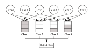
Figure 1: An example of a four-class classification with Max Wins.

2.2 Decision Directed Acyclic Graphs

Platt et al.  [11] introduced a learning algorithm using the Directed Acyclic Graph (DAG) to represent the classification task, called the Decision Directed Acyclic Graph (DDAG). This architecture represents a set of nodes connected by edges with no cycles. Each edge has an orientation and each node has either 0 or 2 edges. Among these nodes, there exists a root node which is the unique node with no edge pointing into it. In a DDAG, the nodes are arranged with a triangular shape in which each node is labeled with an element of a boolean function. There exists a single root node at the top, two nodes in the second layer, and so on until the final layer of $N$ leaves for an $N$-class problem.

To make a classification, an example with an unknown class label is evaluated by the nodes as binary decision functions. The binary output result in each layer is applied to eliminate the candidate output classes and the binary classifiers related to the defeated class are removed. At the first layer (see Fig. 2), the root node can be randomly selected from all possible $N(N-1)/2$ classifiers and there are $N$ candidate output classes. After the root node is tested, its binary result is employed to eliminate the candidate output classes and the binary classifiers corresponding to the defeated class are discarded. In the next layer, the remaining binary classifiers are randomly selected to continue the same process in which some classes are eliminated from the remaining candidate classes. The process is repeated until there is only one class remained which is then assigned as the final output class. This algorithm requires only $N-1$ decision nodes in order to obtain the final answer.

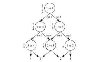
Figure 2: The DDAG finding the best class out of four classes  [11].

One disadvantage of the DDAG is that its classification result is affected by the sequence of binary classifiers randomly selected in the evaluation process. Platt et al. also proposed the other method that prefers the binary decision function with the higher generalization performance measured by its margin sizes, called the large margin DAGs [11]. The margin size ($\Delta$) is a parameter for bounding the generalization ability of the binary SVM as shown in terms of the VC-dimension in Eq. (2). It illustrates that the generalization performance of the binary model is proportional to the size of the margin. A binary classifier with the larger margin size will be firstly applied in each round of the evaluation step. Moreover, Takahashi and Abe [14] proposed a similar framework that employed the number of support vectors as a performance measure. In this method, the generalization error ($\epsilon_{ij}$) for classes $i$ and $j$ was bounded by Eq. (1) [18]:

$$\epsilon_{ij}=\frac{SV_{ij}}{M_{ij}},$$ (1)

where $SV_{ij}$ is the number of support vectors for classes $i$ and $j$ and $M_{ij}$ is the number of training data for classes $i$ and $j$.

2.3 Adaptive Directed Acyclic Graphs

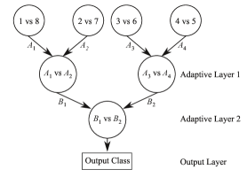
Figure 3: The structure of an adaptive DAG for an 8-class problem.

In the DDAG, binary classification result of a previously employed binary classifier is used to eliminate a candidate output classe, and there are only current remaining candidate classes that can be possibly assigned as the final output class. Therefore, the misclassification of a selected BCRT is the crucial point.

The ADAG was originally designed to reduce this risk of the DDAG by using reversed triangular structure [13]. In an $N$-class problem, there are $\lceil\frac{N}{2}\rceil$ nodes at the top, $N/2^{2}$ nodes in the second layer and so on until the lowest layer of the final node, as illustrated in Fig. 3. Like the DDAG, binary output results of the ADAG in each layer are applied to discard candidate output classes and the binary classifiers related to the defeated classes are also ignored. Therefore, the ADAG also evaluates only $N-1$ nodes to obtain the final answer.

According to the critical issue of misclassification mentioned above, even only one selected classifier related to the target class provides a wrong answer, the misclassification on the final output class cannot be avoided. Hence, the number of times the target class is tested against other classes indicates the risk of misclassification. The DDAG requires at most $N-1$ times that the target class is tested against other classes, while the ADAG requires only $\lceil log_{2}N\rceil$ times or less. This shows that the opportunities of the target class tested against other classes on the ADAG is much lower than the DDAG.

3 An Estimation of the Generalization Performan-ces of Binary Support Vector Machines

The generalization performance of a learning model is the actual performance evaluated on unseen data. For support vector machines, a model is trained by using the concept of the Structure Risk Minimization principle [19] in which the generalization performance of the model is estimated based on both terms of the complexity of model (the VC dimension of approximating functions) and the quality of fitting training data (empirical error). Consider the problem of binary classification where dataset $X$ of $m$ samples in real $n$-dimensional space is randomly independent identically distributed observations drawn according to $P(x,y)=P(x)P(y|x)$. The expected risk ($R(\alpha)$) with probability at least $1-\delta$ can be bounded by the following equation [20, 21]:

$$R(\alpha)\leq\frac{l}{m}+\sqrt{\frac{c}{m}({\frac{R^{2}}{\Delta^{2}}{log^{2}m}+log{\frac{1}{\delta}}})},$$ (2)

where there is a corresponding constant $c$ for all probability distributions, $l$ is the number of labeled examples in $z$ with margin less than $\Delta$, $R$ indicates the radius of the smallest sphere that contains all the data points, and $\Delta$ is the distance between the hyperplane and the closest points of the training set (margin size). The first and second terms of inequality in Eq. (2) denote the bound of the empirical error, and the VC dimension, respectively.

In our frameworks, the generalization ability will be applied to improve the multi-class classification. Although there have been many attempts to use some performance measures such as the margin size [11], the number of support vectors [14], they may not accurately reflect the actual performance of each binary SVM. Consider a two-class problem where hyperplanes $h_{1}$ and $h_{2}$ are learning models created to separate the positive and the negative examples. Suppose that they provide different margin sizes of $\Delta_{1}$ and $\Delta_{2}$, and the different numbers, $l_{1}$ and $l_{2}$, of labeled examples in $z$ with the margin less than their margin sizes, respectively. In case that the parameters $c$ and $\delta$ are fixed, there are only two parameters including $\Delta$ and $l$ that affect the performance of the learning model (as the parameters $m_{1}$ and $m_{2}$, as well as $R_{1}$ and $R_{2}$ are the same for the same pair of a two-class problem). Now consider two-learning models learned from different pairs of a two-class problem. In case that the parameters $c$, and $\delta$ are fixed, according to inequality in Eq. (2), obviously, if we use only $\Delta$, $\l$, or combination of them, they are not sufficient to represent the whole term of their generalization abilities. This shows that a binary model with the larger margin size may not provide more accurate result of classification. The use of only the number of support vectors is also shown in [21] that it is not predictive for generalization ability.

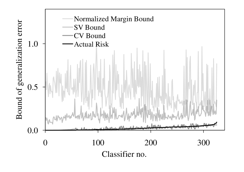
(a)

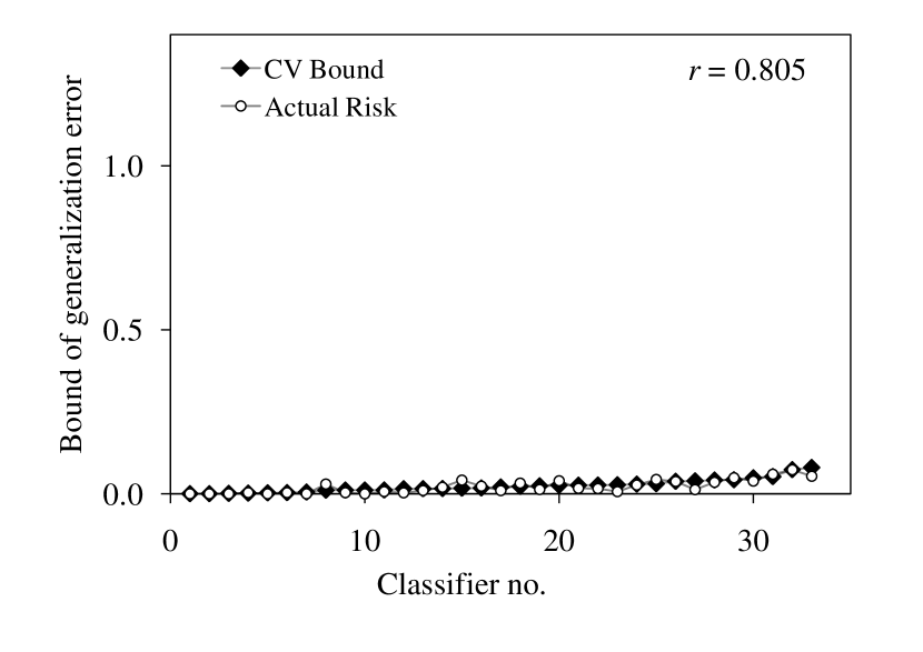
(b)

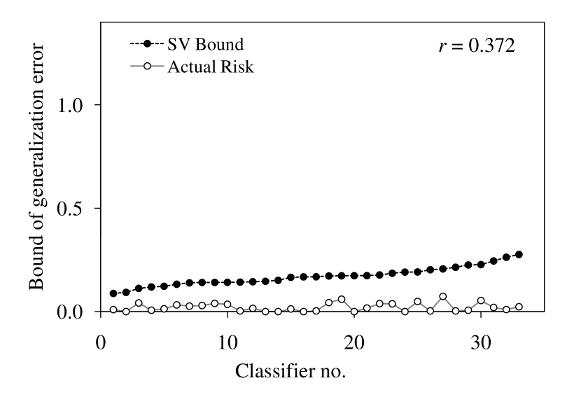
(c)

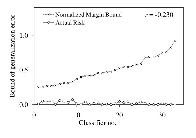
(d)

Figure 4: Generalization errors of 325 classifiers of the Letter dataset based on $k$-fold cross-validation (CV Bound), the number of support vectors (shown in term of the ratio between the number of support vectors and the number of training data: SV Bound), the margin size (shown in term of its inverse value normalized to be in [0,1]: Normalized Margin Bound), and their actual risks on test data (unseen data) by applying the polynomial kernel of $d=4$. Figure (a) compares generalization errors calculated by all techniques where classifiers are sorted in the ascending order by their actual generalization performances (actual risk), and figures (b)-(d) show the comparisons between the actual risks, and the estimated generalization errors with different measures, i.e., CV Bound, SV Bound, and Normalized Margin Bound, respectively (the classifiers will be sorted in ascending order by the estimated generalization errors, and for ease of visualization we show only $10\%$ of classifiers by sampling every ten classifers from the sorted list of the classifiers.

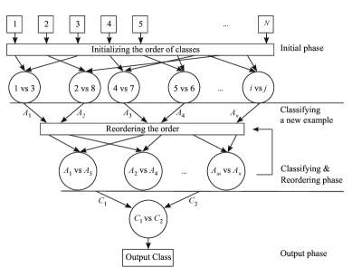
Figure 5: Classification process of the RADAG.

As described above, the generalization ability can be employed to enhance the performance of multi-class classification, by carefully design algorithms which utilize this information as a selection measure for good classifiers. We believe that the generalization performance of binary SVMs can be directly estimated by $k$-fold cross-validation  [22] (see Algorithm 1), and it can be used to fairly compare the performances of binary SVMs on different two-class problems. Below we give an example which demonstrates that $k$-fold cross-validation is more suitable for estimating the generalizaiton performance of the classifiers than the other measures used by the previous methods, i.e. the number of support vectors, the margin size.

Algorithm 1 An estimation of the generalization error of a classifier by using $k$-fold cross-validation.

1:procedure Cross Validation

2:     Set of training data $T$ is partitioned into $k$ disjoint      equal-sized subsets

3:     Initial the classification error of round $i$: $\epsilon_{i}\leftarrow 0$

4:     for $i$=1 to $k$  do

5:         validate set $\leftarrow$ $i^{th}$ subset

6:         training set $\leftarrow$ all remaining subsets

7:         Learn model based on training set

8:         $\epsilon_{i}$ $\leftarrow$ Evaluate the learned model by validate set, and find the number of examples with misclassification

9:     end for

10:     generalization error $\leftarrow$ $\sum_{i=1}^{k}\epsilon_{i}\times\frac{1}{|T|}$

11:     return generalization error

12:end procedure

Fig. 4 shows the generalization performance measured by the previous methods  [11, 14], and $k$-fold cross-validation, which we propose to use as the performance measure, for the Letter dataset with 26 classes, by applying the polynomial kernel of $d=4$. Fig. 4 (a) illustrates that the trend of estimated generalization error by $k$-fold cross-validation is very closed to the actual risk, while the other two techniques give high variation. To further investigation in more details, we select about $10\%$ of all classifiers to show in Fig. 4 (b-d); these figures illustrate the comparisons between the actual risk and the estimated generalization errors with different measures, i.e., CV Bound, SV Bound, and Normalized Margin Bound, respectively. In each figure, classifiers are sorted in ascending order by the estimated generalization errors. It is expected that if a specific measure is a good estimator for generalization error, its value should be in the same trend as the actual risk (its value shoud increase with the increase of the actual risk). A good trend is found in Fig. 4 (b), while the other two methods give no clear trend and contain confusing patterns. In order to evaluate the efficiency of these estimating methods, we apply the correlation analysis between two variables [23], i.e., the actual risks and these three estimated generalization errors. These evaluations are based on 325 classifiers as in Fig. 4 (a), and the statistical r-values of them are 0.805, 0.372, and -0.230 as shown in Fig. 4 (b-d), respectively. The r-values also confirm that CV Bound and actual risk have high correlation, while the other two methods give very low correlation. They show that $k$-fold cross-validation is more suitable to be the measure for the performance of binary classifiers. According to the above reason, we apply this measure in our research.

4 The proposed methods

The combination of binary SVMs with high generalization performance directly affects the accuracy of the multi-class classification. In this section, we introduce four enhanced approaches based on the previous techniques i.e., the ADAG, the DDAG, and Max Wins by applying the generalization abilities in order to select suitable binary classifiers. An improvement of the ADAG is called the Reordering Adaptive Directed Acyclic Graph (RADAG). There are two improved versions for the DDAG i.e., Strong Elimination of the classifiers (SE) and Weak Elimination of the classifiers (WE). The last technique is Voting-based Candidate Filtering (VCF) enhanced from Max Wins. To increase the classification accuracy, the generalization estimated by $k$-fold cross-validation is utilized as the goodness measure of classifiers in our frameworks.

4.1 Reordering Adaptive Directed Acyclic Graph

The ADAG is designed to reduce the number of times the binary classifiers related to the target class are applied, from at most $N-1$ times required by the DDAG, to $\lceil log_{2}N\rceil$ times or less. However, binary classifiers in the first level of the ADAG are still randomly selected, and its misclassification can be produced at the time even when only one BCRT gives a wrong answer. In this section, we introduce a more effective method which uses the minimum weight perfect matching to select the optimal pairs of classes in each level with minimum generalization error. We called the method the Reordering Adaptive Directed Acyclic Graph (RADAG).

The structure of the RADAG is similar to the ADAG, but they are different in the initialization of the binary classifiers in the top level and the order of classes in lower levels (see Fig. 4.1). The reordering algorithm with minimum weight perfect matching is described in Algorithm 2. The algorithm selects the optimal order of classes in each level. It is different from the ADAG in that the initial order of classes in the ADAG is obtained randomly, and the matching of classes in successive levels depends on the classification results of nodes from the previous level. For the RADAG, the reordering process will be applied to the remaining candidate classes in all levels for determining the optimal sequence of them.

Figure 6: (a) A graph for an 8-class problem (b) An example of the output of the reordering algorithm.

To select the optimal set of classifiers, the generalization measure in Section 3 is used as a criterion. This scheme provides less chance to predict the wrong class from all possible $\frac{N!}{2^{\lfloor{N/2}\rfloor}{\lfloor{N/2}\rfloor}!}$ orders. Among $N(N-1)/2$ classifiers, $N/2$ classifiers which have the smallest sum of generalization errors will be used in the classification.

Algorithm 2 Reordering Adaptive Directed Acyclic Graph (RADAG).

1:procedure RADAG

2:     Initial set of candidate output classes $C=\{1,2,3,...,N\}$, and set of discarded classes $D=\emptyset$

3:     Calculate generalization errors of all possible pairs of classes on $C$ as described in Section 3

4:     Create the binary SVMs from all possible pairs of classes on $C$

5:     while $|C|>1$ do

6:         Apply the minimum weight perfect matching [24] to find the optimal $\lfloor\frac{|C|}{2}\rfloor$ pairs of classes from all possible          pairs on $C$ to obtain the optimal binary models with minimum generalization error

7:         $D$ $\leftarrow$ Classify the example by the optimal binary models, and find the defeated classes

8:         $C$ $\leftarrow$ $C-D$

9:     end while

10:     final output class $\leftarrow$ the last remaining candidate class

11:     return final output class

12:end procedure

Let $G=(V,E)$ be a graph with node set $V$ and edge set $E$. Each node in $G$ denotes one class and each edge indicates one binary classifier of which generalization error is estimated from Section 3 (see Fig. 6(a)). The output of the reordering algorithm for graph $G$ is a subset of edges with the minimum sum of generalization errors of all edges and each node in $G$ is met by exactly one edge in the subset (see Fig. 6(b)).

Given a real weight $\epsilon_{e}$ being generalization error for each edge $e$ of $G$, the problem of reordering algorithm can be solved by the minimum weight perfect matching [24] that finds a perfect matching $M$ of minimum weight $\sum(\epsilon_{e}:e\in M)$.

For $U\subseteq V$, let $E(U)=\{(i,j):(i,j)\in E,i\in U,j\in U\}$. $E(U)$ is the set of edges with both endpoints in $U$. The set of edges incident to node $i$ in the node-edge incidence matrix is denoted by $\delta(i)$. The convex hull of perfect matchings on a graph $G=(V,E)$ with $|V|$ even is given by
      a) $x\in\{0,1\}^{m}$
      b) $\sum_{e\in\delta(v)}x_{e}=1$ for $v\in V$
      c) $\sum_{e\in E(U)}x_{e}\leq\lfloor\frac{|U|}{2}\rfloor$ for all odd sets $U\subseteq V$ with $|U|\geq 3$ or by (a),(b) and
      d) $\sum_{e\in\delta(U)}x_{e}\geq 1$ for all odd sets $U\subseteq V$ with $|U|\geq 3$
where $|E|=m$, and $x_{e}=1$ ($x_{e}=0$) means that $e$ is (is not) in the matching.

Hence, the minimum weight of a perfect matching is at least as large as the value of

$$min\sum_{e\in E}\epsilon_{e}x_{e}$$ (3)

where $x$ satisfies “(a), (b), and (c)”  or “(a), (b) and, (d)”. Therefore, the reordering problem can be solved by the integer program in Eq. (3).

4.2 Strong & Weak Elimination of Classifiers for Enhancing Decision Directed Acyclic Graph

Algorithm 3 Strong Elimination of the classifiers (SE).

1:procedure SE

2:     Initial set of candidate output classes $C=\{1,2,3,...,N\}$, and set of discarded classes $D=\emptyset$

3:     Calculate generalization errors of all possible pairs of classes on $C$ as described in Section 3

4:     Create the binary models from all possible pairs of classes on $C$

5:     Sort the list of the binary models in ascending order by the generalization errors

6:     current classifier $\leftarrow$ the first element on the sorted list

7:     while $|C|>1$ do

8:         $D$ $\leftarrow$ Classify the example by the current classifier, and find the defeated class

9:         $C$ $\leftarrow$ $C-D$

10:         current classifier $\leftarrow$ the next element on the sorted list where it is not related to any classes discarded                                       from $C$

11:     end while

12:     final output class $\leftarrow$ the last remaining candidate class

13:     return final output class

14:end procedure

Algorithm 4 Weak Elimination of the classifiers (WE).

1:procedure WE

2:     Initial set of candidate output classes $C=\{1,2,3,...,N\}$, and set of discarded classes $D=\emptyset$

3:     Calculate generalization errors of all possible pairs of classes on $C$ as elaborated in section 3

4:     Create the binary models from all possible pairs of classes on $C$

5:     Sort the list of the binary models in ascending order by the generalization errors

6:     current classifier $\leftarrow$ the first element on the sorted list

7:     while $|C|>1$ do

8:         $D$ $\leftarrow$ Classify the example by current classifier, and find the defeated class

9:         $C$ $\leftarrow$ $C-D$

10:         current classifier $\leftarrow$ the next element on the sorted list where it does not include all two classes discarded                                      from $C$

11:     end while

12:     final output class $\leftarrow$ the last remaining candidate class

13:     return final output class

14:end procedure

According to the characteristic of the DDAG, binary classification results of the previously employed binary classifiers are used to eliminate the candidate output classes, and thus the final output class will be assigned with one of the remaining candidate classes. By using the random technique for selecting a binary classifier, the DDAG produces mis-classification at the time when a BCRT with very low performance is selected and provides the wrong answer, as the target class will be discarded from the remaining candidate classes, and it is not possible to reach the correct output class. In this section, we propose the framework to enhance the performance of the DDAG to select the binary classifier with high performance based on the generalization abilities of binary classifiers as described in Section 3.

We propose two methods that are Strong Elimination of the classifiers (SE) and Weak Elimination of the classifiers (WE). Both algorithms are described in Algorithm 3 and Algorithm 4. We also show a classification process of SE and WE for an $N$-class problem in Fig. 7 and Fig. 8, respectively.

For both of the DDAG and SE, in each round, a defeated class will be removed from candidate output classes, and all binary classifiers related to the defeated class are ignored. Due to this reason, they guarantee $N-1$ number of classifications for an $N$-class problem. However, these ignored classifiers may have high generalization abilities and thus are helpful to eliminate the other remaining candidate classes. Therefore, we then propose WE to make use of binary classifiers with high generalization abilities.

According to the classifier elimination of WE, the number of classifications is bounded with the best case of $N-1$, and the worst case of $N(N-1)/2$. However, WE provides the opportunities to employ better classifiers as shown in the Fig. 8. At round $r$, suppose that classifier $A_{i}$ vs $A_{j}$ has lower generalization error than classifier $A_{i}$ vs $A_{k}$ , and both of them are active classifiers. In this case, it is possible that classifier $A_{i}$ vs $A_{j}$ can remove the class $A_{i}$ from the list of two remaining candidate classes, and can avoid using classifier $A_{i}$ vs $A_{k}$ with lower reliability that is unavoidable for SE as shown in Fig. 7.

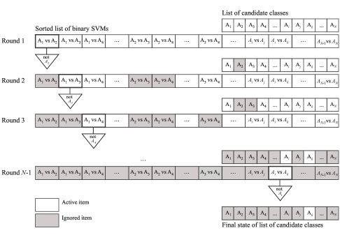
Figure 7: Classification process of SE for an $N$-class problem.

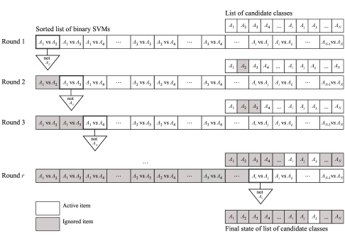
Figure 8: Classification process of WE for an $N$-class problem.

4.3 Voting Based Candidate Filtering

Max Wins is one of high performance techniques that work based on the concept of “trust on the most popular opinion” for making decision to select the output class. If all of $N-1$ BCRTs give the correct answer, Max Wins will always provide the correct output class. It does not depend on the answers of the other binary classifiers. However, if only one of BCRTs gives a wrong answer, it may lead to misclassification due to equal voting, or another non-target class reaching the largest vote. Fig. 9 shows an example of such cases, taken from our experiment on the Letter dataset (see Section  for more details); Fig. 9(a) and (b) show the cases of equal voting and another non-target class having the largest vote, respectively.

We propose a novel multi-class classification approach that alleviates the above problem of Max Wins, and uses the same concept “trust on the most popular opinion” for filtering out the low competitive classes. On the other hand, high competitive classes will be voted to be candidate output classes, though there exist some BCRTs providing the wrong answer. If there is more than one remaining class, the output class will be selected via the mechanism of WE. Our proposed technique aims to combine the strong point of both Max Wins and WE, and is called Voting based Candidate Filtering (VCF). The details of our algorithm are shown in Algorithm 5.

Algorithm 5 Voting based Candidate Filtering (VCF).

1:procedure VCF

2:     Initial set of candidate output classes $C=\{1,2,3,...,N\}$, and score of class $i$: $s_{i\in N}\leftarrow 0$

3:     Create the binary models from all possible pairs of classes on $C$

4:     for $j$=1 to $N(N-1)/2$  do

5:         $w$ $\leftarrow$ Classify the example by classifier $j^{th}$, and find the winner class

6:         $s_{w}$ $\leftarrow$ $s_{w}+1$

7:     end for

8:     $s_{top}$ $\leftarrow$ Find the top voting score of all $s_{i\in N}$

9:     for $i$=1 to $N$  do

10:         $dp_{i}\leftarrow\frac{(s_{top}-s_{i})\times 100}{s_{top}}$

11:         if $dp_{i}\leq$ $threshold\_value$ then

12:              Add class $i$ into the set of candidate output classes $C$

13:         end if

14:     end for

15:     if $|C|>1$ then

16:         final output class $\leftarrow$ Call the WE procedure

17:     else

18:         final output class $\leftarrow$ the last remaining candidate class

19:     end if

20:     return final output class

21:end procedure

Let $s_{top}$, and $s_{i}$ indicate the maximum of scores for all $N$ classes, and the score of class $i\in[N]$ for a test data, respectively. Also let $dp_{i}$ denotes the percentage of the difference between $s_{top}$ and $s_{i}$. An example of the calculation of $dp_{i}$ is shown in Fig. 9 (a), where $i=\textquoteleft$E’, the score of class $\textquoteleft$E’ = 23 points, and the score of class $\textquoteleft$C’ = 24 points (as the top score). Then $dp_{i}$ value can be calculated by $\frac{(24-23)\times 100}{24}=4.17$. We also define $threshold\_value$ to be the threshold of $dp_{i}$ for considering class $i$ as a candidate for the target class; class $i$ will be accepted into the set of high competitive candidate classes if and only if its $dp_{i}$ is less than or equal to $threshold\_value$. We want to keep the size of the filtered candidate classes as small as possible while still containing the target class.

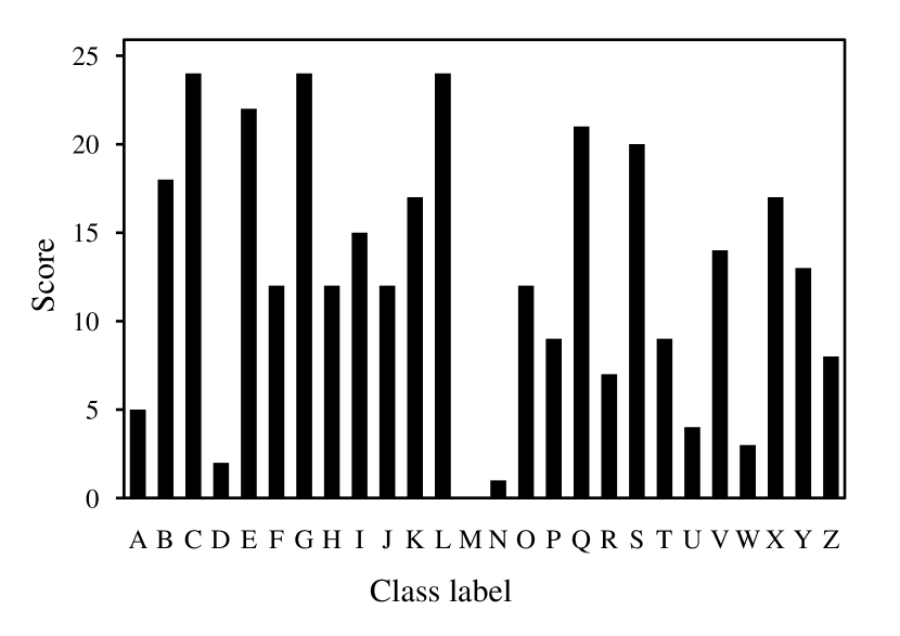
(a)

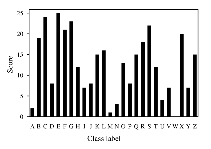
(b)

Figure 9: An example of high risk of misclassification of Max Wins together with score distribution of all classes: two cases of misclassification of class $\textquoteleft$C’ due to only one BCRT giving the wrong answer in the Letter problem having 26 classes (25 possible BCRTs, and 25 points as the largest possible score), a) three classes, including $\textquoteleft$C’, $\textquoteleft$G’, and $\textquoteleft$L’, with equal score (only one BCRT $\textquoteleft$C vs G’ giving the wrong class), and b) the non-target class $\textquoteleft$E’ with the highest score (only one BCRT $\textquoteleft$C vs E’ providing the wrong class).

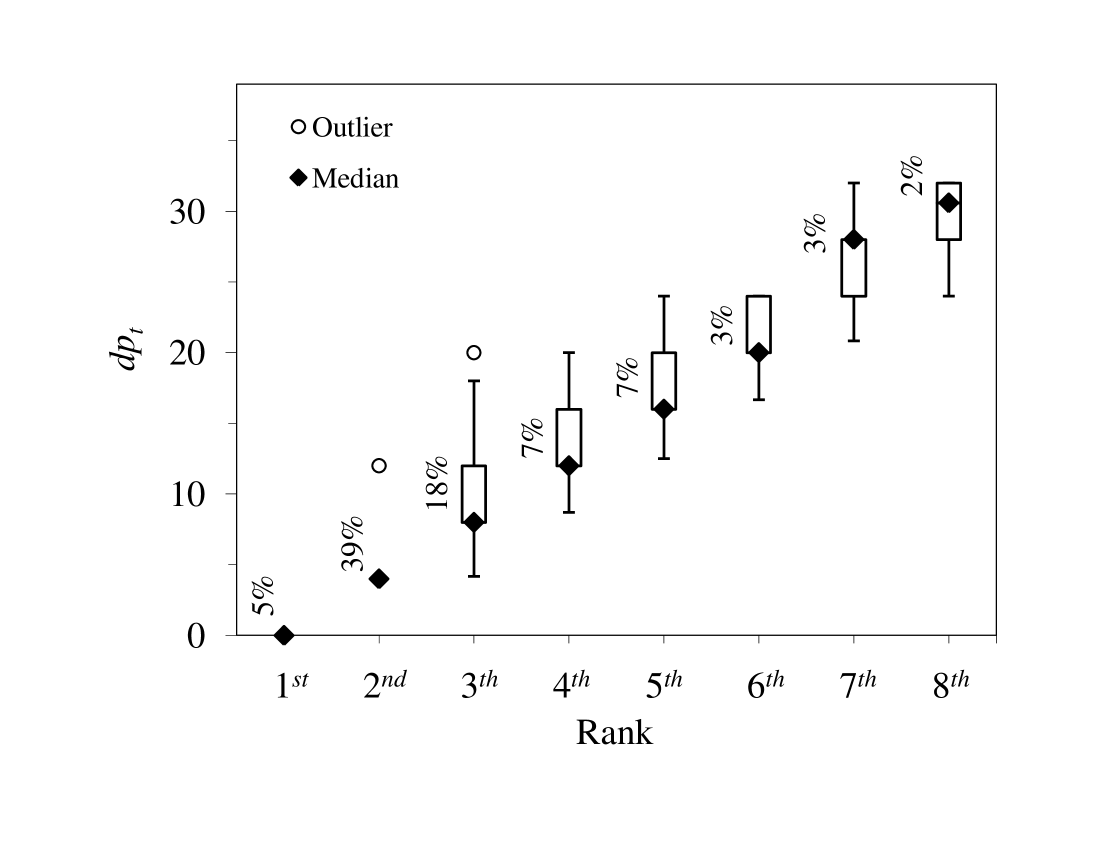
Figure 10: A case study of the $461$ examples with high risk of misclassification in the Letter problem. The maximum voting scores of these examples are reached (1) by both of the target class and the non$-$target class (equal vote: $1^{st}$ rank), or (2) by a non$-$target class (absolutely wrong: $2^{nd}-8^{th}$ rank). The figure shows the target class score of these examples by observing between the $dp_{t}$ and the rank of the target class.

A case study of high risk of misclassification in the Letter dataset including 4,010 examples where Max Wins provides 3,549 examples with the correct result, and 461 examples with high risk of misclassification. By a high-risk example, we mean (1) the example with an equal vote (the score of the target class is equal to those of other non-target classes) and (2) the example with a vote less than the maximum vote that is then mis-classified by Max Wins. These high risk examples will be hopefully recovered with the correct class label by our proposed algorithm. In our experiment, the high-risk examples includes 24 examples (around 5$\%$) with an equal vote, and 437 examples (around 95$\%$) with a vote less than the maximum as shown in Fig. 10, where $dp_{t}$ represents the percentage of the difference between $s_{top}$ and the score of the target class. For each example, we calculate the rank of the voting score of the target class compared to the other non-target classes, and consider only the first eight ranks. There are 24 examples (around $5\%$) in the first rank, while in the second to the eighth ranks, the numbers of examples are 171, 77, 31, 30, 15, 14, and 10 (around $39\%,18\%,7\%,7\%,3\%,3\%$, and $2\%$), respectively. The examples with the different ranks have different ranges of $dp_{t}$ values, such as, in the second rank, the $dp_{t}$ values are varied from $4.0$ to $12.0$, in the third rank, the $dp_{t}$ values are varied from $4.2$ to $20.0$, in the fourth rank, the $dp_{t}$ values are varied from $8.7$ to $20.0$, and so on.

According to this case study, there can be at most $5\%$ of examples that will be correctly classified with the correct class label by random selection of Max Wins, while the other $95\%$ of examples will be absolutely misclassified. We want to recover an example that is not correctly classified by Max Wins, as its actual target class is not in the first rank or its target class has equal vote with some other output classes. If $threshold\_value$ is set as $1$ in the VCF algorithm, it will guarantee that all high-risk misclassified examples with $dp_{t}$ values no greater than can be filtered into the set of the candidate output classes; in this case only the examples in the first rank ($5\%$ of examples) will be selected. When we apply a bigger threshold, e.g. $threshold\_value$ $=10$, it covers all misclassified examples in the first and the second ranks ($5\%+39\%$), almost of the third rank ($18\%$), and some parts of the fourth rank ($7\%$). It shows that the increase of $threshold\_value$ covers more candidate classes, while the larger size of $threshold\_value$ creates a higher risk to employ an unnecessarily large number of binary classifiers. On the other hand, if $threshold\_value$ is too low, the target class may be removed. However, a suitable $threshold\_value$ can be obtained by general tuning techniques. For our experiment, we just define $threshold\_value$ to be $10$ for all of datasets without fine-tuning which is good enough to demonstrate the effectiveness of the VCF algorithm.

5 Experiments

In this section, we design the experimental setting to evaluate the performance of the proposed methods. We compare our methods with the traditional algorithms, i.e., the DDAG, the ADAG, and Max Wins. We divide this section into two parts as experimental protocols, and results & discussions.

5.1 Experimental Protocol

We run experiments on sixteen datasets from the UCI Machine Learning Repository [17] including Page Block, Glass, Segment, Arrhyth, Mfeat-factor, Mfeat-fourier, Mfeat-karhunen, Mfeat-zernike, Optdigit, Pendigit, Primary tumor, Libras Movement, Abalone, Krkopt, Spectrometer, and Letter (see Table 1). For the datasets containing both training data and test data, we added up both of them into one set, and used 5-fold cross validation for evaluating the classification accuracy.

Table 1: Description of the datasets used in the experiments.

Datasets	#Cases	#Classes	#Features
Page Block	5,473	5	10
Glass	214	6	9
Segment	2,310	7	18
Arrhyth	438	9	255
Mfeat-factor	2,000	10	216
Mfeat-fourier	2,000	10	76
Mfeat-karhunen	2,000	10	64
Mfeat-zernike	2,000	10	47
Optdigit	5,620	10	62
Pendigit	10,992	10	16
Primary tumor	315	13	15
Libras Movement	360	15	90
Abalone	4,098	16	8
Krkopt	28,056	18	6
Spectrometer	475	21	101
Letter	20,052	26	16

In these experiments, we scaled data to be in [-1,1] and employed two kernel functions i.e., the Polynomial kernel $K(x_{i},x_{j})\equiv|({\bf x_{i}}\cdot{\bf x_{j}}+1)|^{d}$, and the RBF kernel $K(x_{i},x_{j})\equiv e^{-\gamma||{\bf x_{i}}-{\bf x_{j}}||^{2}}$. For the polynomial kernel we applied the same set of degrees $d=\{2,3,4,5\}$ to all datasets, and for the RBF kernel we applied the set of degrees $\gamma_{1}=\{1,0.5,0.1,0.05\}$ to Page Block, Glass, Segment, Mfeat-zernike, Pendigit, Libras Movement, Abalone, Krkopt, and Letter, and applied the set of degrees $\gamma_{2}=\{0.1,0.05,0.01,\\ 0.005\}$ to the other datasets. The default parameter of regularization parameter $C$ was used for model construction; this parameter is used to trade off between error of the SVM on training data and margin maximization. In the training phase, we used software package $SVM^{light}$ version 6.02 [25, 26] to create the $N(N-1)/2$ binary classifiers. For the DDAG and the ADAG, we examined all possible orders of classes for datasets having not more than 8 classes, whereas we randomly selected 50,000 orders for datasets having more than 8 classes, and we then calculated the average of accuracy of these orders.

5.2 Results & Discussions

We compare the original methods with their enhanced techniques in three tasks including: (1) the ADAG with the RADAG, (2) the DDAG with two improved approaches, i.e., SE and WE, and (3) Max Wins with VCF.

We also selected the best techniques from (1) and (2), i.e., the RADAG and WE, respectively, and compared them with Max Wins as the state of the art technique. These comparison results are shown in Table 2 to Table 5. Moreover, paired comparison among all of three traditional methods (the DDAG, the ADAG, and Max Wins), and all proposed techniques (SE, the RADAG, WE, and VCF) are concluded in Table 6.

The best accuracy among these methods is represented in bold-face. In addition, we used the one-tailed paired t-test technique to analyze the significant difference between the accuracies of the traditional algorithms and the proposed algorithms. To estimate the difference between accuracies, we use a $k$-fold cross-validation method [22].

To indicate the level of the confidence interval using a one-tailed paired t-test in the Table 2 to Table 5, the symbol ‘$+$’ and ‘$-$’ are used to represent that the corresponding method has higher accuracy, and lower accuracy compared to a baseline method, respectively. The number of symbols shows the level of confidence interval for estimating the difference between accuracies of two algorithms i.e., one symbol, two symbols, and three symbols represent 90%, 95%, and 99% respectively.

Table 2: A comparison of the classification accuracy of the ADAG and the RADAG.

	Polynomial			RBF
Data sets	ADAG	RADAG		ADAG	RADAG
Page Block	93.597	93.541 $---$		93.562	93.555 $-$
Glass	63.879	64.019		63.084	63.318
Segment	93.207	93.236$+{\color[rgb]{1,1,1}*}$		93.348	93.366
Arrhyth	63.489	63.470		58.049	57.991
Mfeat-factor	97.238	97.225 $--{\color[rgb]{1,1,1}*}$		96.921	96.938
Mfeat-fourier	82.839	82.863		82.456	82.513$+$
Mfeat-karhunen	96.864	96.863		96.890	96.900
Mfeat-zernike	82.368	82.413$+++{\color[rgb]{1,1,1}*}$		81.867	81.888
Optdigit	98.995	98.999		98.620	98.630
Pendigit	99.400	99.402		99.313	99.320$+$
Primary tumor	47.266	47.619$++{\color[rgb]{1,1,1}*}$		46.089	46.429$+++$
Libras Movement	73.218	73.194		72.289	72.569$+$
Abalone	27.603	27.648		27.353	27.337
Krkopt	53.102	53.239$+++$		53.088	53.173$+++$
Spectrometer	54.445	54.842$++{\color[rgb]{1,1,1}*}$		50.808	51.579$+{\color[rgb]{1,1,1}*}$
Letter	88.668	88.787$+++$		89.989	90.090$+++$

The experimental results in Table 2 uses the ADAG as the baseline algorithm. It shows that the RADAG yields highest accuracy in several datasets. The results also show that, at $95$% confidence interval, the RADAG performs statistically better than the ADAG in five datasets using the Polynomial kernel and better in three datasets using the RBF kernel. As shown in the table, the RADAG performs better when the number of classes is comparatively large, and does not perform well in the datasets with the small number of classes, i.e., the Page Block, and the Mfeat-factor with 5 and 10 classes, respectively. We believe that in case of datasets with the large number of classes, the variety of generalization errors of classifiers in consideration is rich and the RADAG is able to choose good classifiers freely, whereas the RADAG may be forced to select ineffective classifiers in case of the small number of classes, and it could lead to an incorrect output class.

Table 3: A comparison of the classification accuracy between the DDAG, and our methods, i.e, SE, and WE.

	Polynomial					RBF
Data sets	DDAG		SE	WE		DDAG		SE	WE
Page Block	93.597		93.541 $---$	93.623$+$		93.562		93.555 $-$	93.582$++{\color[rgb]{1,1,1}*}$
Glass	63.892		64.019	64.019		63.084		63.201	63.201
Segment	93.207		93.236 $+$	93.247$++$		93.350		93.344	93.366
Arrhyth	63.490		63.527	63.527		58.048		57.991	58.162
Mfeat-factor	97.238		97.250	97.238		96.923		96.975$+$	96.975$++{\color[rgb]{1,1,1}*}$
Mfeat-fourier	82.837		82.863	82.863		82.443		82.475	82.538
Mfeat-karhunen	96.863		96.875	96.875		96.861		96.850	96.988$+{\color[rgb]{1,1,1}*}$
Mfeat-zernike	82.362		82.400$++{\color[rgb]{1,1,1}*}$	82.350		81.869		81.888	81.863
Optdigit	98.994		99.013$++{\color[rgb]{1,1,1}*}$	99.008 $+{\color[rgb]{1,1,1}*}$		98.618		98.643$+$	98.630
Pendigit	99.399		99.404	99.402		99.312		99.318	99.320$+$
Primary tumor	47.227		47.064	47.460$++$		46.019		46.032	46.111
Libras Movement	73.142		73.264	73.472$++{\color[rgb]{1,1,1}*}$		72.283		72.569$+$	72.431
Abalone	27.611		27.648	27.672$+$		27.354		27.330	27.398
Krkopt	53.101		53.263 $++$	53.472$+++$		53.088		53.212 $+++$	53.320$+++$
Spectrometer	54.373		54.632	54.421		50.821		51.316	51.842$++$
Letter	88.609		88.707 $+++$	88.835$+++$		89.903		89.977 $++$	90.294$+++$

Table 3 shows the experimental results of SE and WE compared with the DDAG as the baseline algorithm. Both WE and SE have higher accuracy than the traditional DDAG in almost all datasets. The results also show that at $95$% confidence interval, SE performs statistically significantly better than the DDAG in four datasets using the Polynomial kernel and significantly better than the DDAG in two datasets using the RBF kernel. It is similar to the previous comparison between the ADAG and the RADAG that in datasets with the small number of classes, the classifier manipulation of SE may be forced to select inaccurate classifiers and it possibly leads to the misclassification. The results also show that WE performs statistically significantly better than the DDAG in five datasets in both cases of the Polynomial kernel and the RBF kernel. These results illustrate that WE can reduce the risk of selecting inaccurate classifiers compared to SE.

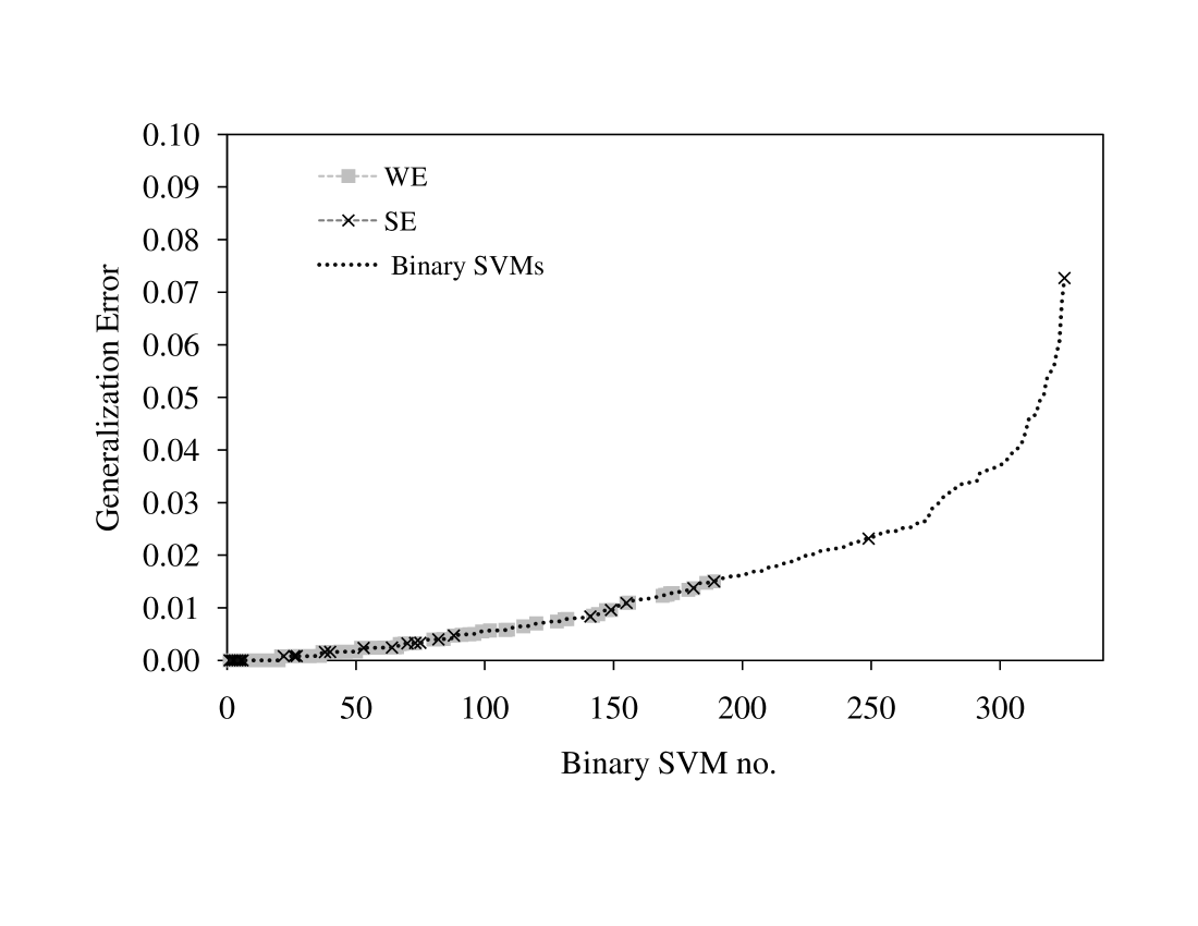
Figure 11: An example of generalization errors of binary SVMs used by WE and SE in the Letter dataset.

Table 4: A comparison of the classification accuracy of Max Wins and VCF.

Data sets	Polynomial			RBF
	Max Wins	VCF		Max wins	VCF
Page Block	93.600	93.623		93.567	93.582$++{\color[rgb]{1,1,1}*}$
Glass	63.863	64.019		63.143	63.201
Segment	93.209	93.247$++{\color[rgb]{1,1,1}*}$		93.351	93.366
Arrhyth	63.489	63.527		58.048	58.162
Mfeat-factor	97.242	97.238		96.927	96.975$++{\color[rgb]{1,1,1}*}$
Mfeat-fourier	82.852	82.825		82.454	82.525
Mfeat-karhunen	96.879	96.875		96.952	96.963
Mfeat-zernike	82.338	82.350		81.825	81.863
Optdigit	99.004	99.013		98.631	98.630
Pendigit	99.402	99.402		99.315	99.320
Primary tumor	47.394	47.460		46.508	46.191
Libras Movement	73.194	73.472$++{\color[rgb]{1,1,1}*}$		72.373	72.431
Abalone	27.614	27.672$+$		27.375	27.398
Krkopt	53.149	53.475$+++$		53.146	53.328$+++$
Spectrometer	54.263	54.421$+{\color[rgb]{1,1,1}*}$		51.026	51.842$++$
Letter	88.706	88.869$+++$		90.112	90.316$+++$

Table 5: A comparison of the classification accuracy between Max Wins and the RADAG, and WE.

	Polynomial				RBF
Data sets	Max Wins	RADAG	WE		Max Wins	RADAG	WE
Page Block	93.600	93.541 $---$	93.623		93.567	93.555 $--{\color[rgb]{1,1,1}*}$	93.582$++{\color[rgb]{1,1,1}*}$
Glass	63.863	64.019	64.019		63.143	63.318	63.201
Segment	93.209	93.236 $+{\color[rgb]{1,1,1}*}$	93.247$++$		93.351	93.366	93.366
Arrhyth	63.489	63.470	63.527		58.048	57.991	58.162
Mfeat-factor	97.242	97.225 $---$	97.238		96.927	96.938	96.975$++{\color[rgb]{1,1,1}*}$
Mfeat-fourier	82.852	82.863	82.863		82.454	82.513	82.538
Mfeat-karhunen	96.879	96.863	96.875		96.952	96.900	96.988
Mfeat-zernike	82.338	82.413$++{\color[rgb]{1,1,1}*}$	82.350		81.825	81.888$++{\color[rgb]{1,1,1}*}$	81.863
Optdigit	99.004	98.999	99.008		98.631	98.630	98.630
Pendigit	99.402	99.402	99.402		99.315	99.320	99.320
Primary tumor	47.394	47.619$++$	47.460		46.508	46.429	46.111
Libras Movement	73.194	73.194	73.472$++{\color[rgb]{1,1,1}*}$		72.373	72.569	72.431
Abalone	27.614	27.648	27.672$+$		27.375	27.337	27.398
Krkopt	53.149	53.239 $++{\color[rgb]{1,1,1}*}$	53.472$+++$		53.146	53.173	53.320$+++$
Spectrometer	54.263	54.842$++$	54.421 $+$		51.026	51.579	51.842$++$
Letter	88.706	88.787 $++{\color[rgb]{1,1,1}*}$	88.835$+++$		90.112	90.090	90.294$+++$

We further analyze the results comparing WE and SE on the Letter dataset which consists of $26$ classes and 325 binary learners, as shown in Fig. 11. These 325 classifiers in the figure are sorted in ascending order by the generalization error, and this sequence of classifiers is maintained in the classification phase. SE requires $25$ classifiers and WE requires $93$ classifiers in this case, and the generalization error of the worst binary classifier in WE is almost five times lower than in SE (the largest generalization errors of all binary SVMs used in SE and WE are 0.015, 0.073, respectively). As a result, the average performance of the binary classifiers in WE is higher than SE.

As shown in Table 4 with Max Wins as the baseline method, VCF yields higher accuracy than Max Wins in almost all of datasets. The results show that, at $95$% confidence interval, in the Polynomial kernel VCF performs statistically significantly better than Max Wins in four datasets, and in the RBF kernel VCF performs statistically significantly better than Max Wins in five datasets. The previous three tables show that our proposed methods improve the accuracy of the ADAG, the DDAG, and Max Wins significantly.

Next, we select the best algorithm in each table from the first two tables, i.e, the RADAG, and WE, and then compare them to Max Wins. According to experimental result in Table 5, at $95$% confidence interval, the RADAG performs statistically significantly better than Max Wins in five datasets using the Polynomial kernel, and significantly higher than Max Wins in one dataset using the RBF kernel. In case of the small number of classes, it is possible that the RADAG will have the effect mentioned above. For WE, the results show that it performs statistically significantly better than Max Wins in four datasets in case of the Polynomial kernel and significantly better than Max Wins in five datasets in case of the RBF kernel. There is no any dataset in which Max Wins has significantly higher accuracy than WE.

Table 6: Paired comparisons among all techniques including of three traditional techniques (DDAG, ADAG, and Max Wins), and four proposed techniques (RADAG, SE, WE, and VCF).

		Traditional Methods				Proposed Methods
Kernel Function	Algorithms	DDAG	ADAG	Max Wins		SE	RADAG	WE	VCF
Polynomial	DDAG		1-15-0	2-14-0		4-11-1	5-9-2	5-11-0	6-10-0
	ADAG			2-13-1		4-11-1	5-9-2	4-12-0	5-11-0
	Max Wins					3-12-1	5-9-2	4-12-0	4-12-0
	SE						2-14-0	4-11-1	4-11-1
	RADAG							2-12-2	4-10-2
	WE								1-15-0
RBF	DDAG		2-14-0	2-14-0		2-14-0	3-13-0	5-11-0	5-11-0
	ADAG			2-14-0		1-15-0	3-13-0	5-11-0	5-11-0
	Max Wins					2-12-2	1-14-1	5-11-0	5-11-0
	SE						2-13-1	4-12-0	3-13-0
	RADAG							3-13-0	3-13-0
	WE								1-15-0

Table 6 summarizes paired comparisons of all algorithms including the traditional techniques, and the proposed works based on both of the Polynomial kernel and the RBF kernel. We show the win-draw-loss record (s) of the algorithm in the column against the algorithm in the row. A win-draw-loss record reports how many datasets the method in the column is better than the method in the row (win), is equal (draw), or is worse (loss) at $95$% confidence interval. As summarized in the table, our proposed methods are better than all previous works i.e., the DDAG, the ADAG, and Max Wins. WE and VCF give the highest accuracy among all of our methods. The result also shows that VCF gives a little better results compared to WE. However, as mentioned before in Section 4.3, the accuracies of VCF are the ones without fine-tuning, and higher accuracies can be expected if fine-tuning is performed to find the optimal $threshold\_value$ for VCF.

5.3 Computational Time

The computational times of all methods are shown in Fig. 12 and Fig. 13. We can classify algorithms according to the time requirement into three groups, for an $N$-class problem: 1) $N-1$ times i.e., the DDAG, the ADAG, SE, and the RADAG, 2) average about half of time of $N(N-1)/2$ i.e., WE, 3) $N(N-1)/2$ i.e., Max Wins, and VCF.

The results show that algorithms in the first and the second groups require comparatively low running time in all datasets, especially when the number of classes is relatively large, while the larger the number of classes, the more running time the algorithms in the third group requires. WE in the second group requires $N-1$ classifiers in the best case and $N(N-1)/2$ classifiers in the worst case; however, in our experimental results WE takes approximately half of time required by the algorithms in the third group. For the RADAG, though the number of classes affects the running time for reordering process, it takes a little time even when there are many classes. The algorithms in the third group need $O(N^{2})$ comparisons for a problem with $N$ classes. VCF needs more time to choose the final class from the set of candidate classes which can be obtained by re-using the previous results of binary classification.

The DDAG reduces the number of comparisons down to $O(N)$. SE spends a little time more than the DDAG for sorting the classifiers in the training phase. By reducing the depth of the path, the ADAG and SE require $O(N)$ comparisons of binary classifiers. WE consumes more time than SE due to each round of classification can reduce only one classifier while SE can eliminate all classifiers built from the discarded class. The number of testing classifiers for WE is equal to that for Max Wins in the worst case; fortunately, the experimental results show that WE actually spends only half of Max Wins’ times in the average case. The RADAG needs a little time more than the ADAG for reordering the order of classes. Note that, the minimum weight perfect matching algorithm, which is used in the reordering algorithm, runs in time bounded by $O(N(M+NlogN))$ [24], where $N$ is the number of nodes (classes) in the graph and $M=N(N-1)/2$ is the number of edges (binary classifiers). The RADAG will reorder the order of classes in every level, except for the last level. The order of classes in the top level is reordered only once and we use the order to evaluate every test example. Hence for classifying each test data, we need $log_{2}N-2$ times of reordering, where each time the number of classes is reduced by half. Therefore, the running time of the RADAG is bounded by $O(c_{1}N)+O(c_{2}N^{3}log_{2}N)$, where $c_{1}$ is much larger than $c_{2}$.

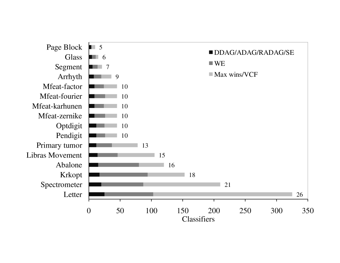
Figure 12: A comparison of the computational time using the Polynomial kernel.

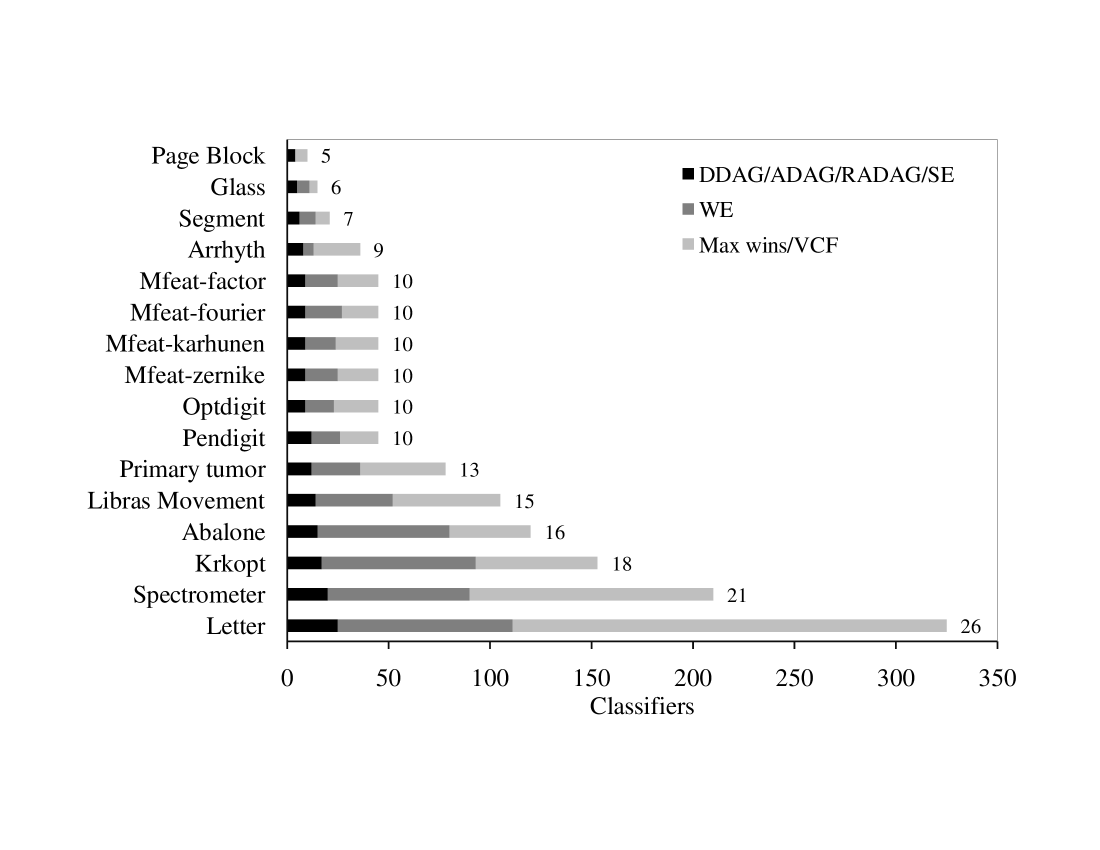
Figure 13: A comparison of the computational time using the RBF kernel.

6 Conclusion

Max Wins is a powerful combining technique with a need of $N(N-1)/2$ number of classifications for an $N$-class problem, while the DDAG and the ADAG reduce the number of classifications to $N-1$. We study the characteristics of these previous methods that lead to wrong classification results. We believe that the performances of them depend on the BCRTs. In case of Max Wins, if there exists only one BCRT giving an incorrect answer, it may convey misclassification due to equal voting or another non-target class reaching the largest vote, while in cases of the DDAG and the ADAG, if only one of BCRTs in the sequence of selected classifiers makes a mistake, the whole system will give the wrong output. We investigate the well-organized combination of the binary models including BCRTs in classification process to provide a more precise final result.

In this research, we propose four methods for overcoming the above weakness of the previous works. All our proposed methods are based on the same principle that if the information about genearalization ability is accurately measured, then it is able to be employed for enhancing the performance of the classification. In this paper, the generalization performance is estimated by $k$-fold cross-validation technique, and we show that it is more suitable than previously used measures in other frameworks, such as the margin size and the number of support vectors. Our proposed methods are the Reordering Adaptive Directed Acyclic Graph (RADAG), Strong Elimination of the classifiers (SE), Weak Elimination of the classifiers (WE), and Voting based Candidate (VCF). The RADAG is an enhanced version for the ADAG by using the minimum weight perfect matching for selecting the optimal pair of classes in each level with minimum generalization error. Compared to the ADAG, the RADAG is not only superior in terms of accuracy, but also maintains the same testing time ($N-1$). Next, We propose two improved algorithms for the DDAG, i.e. SE and WE. In SE, a sequence of binary classifiers selected by minimum generalization error is applied to eliminate the candidate classes until only one class remained and assigned as the final output class. SE provides better accuracy than the DDAG. The testing time of SE is the same as the traditional DDAG and the RADAG, with a number of applied classifiers equal to $N-1$. We also propose the other enhanced version for the DDAG, called WE. This approach aims to efficiently use as many as possible of the classifiers with low generalization errors. This is different from the process of the DDAG and SE in which all binary classifiers related to a defeated class are ignored when the defeated class is removed from the candidate classes. In WE, however, a classifier will be ignored only if all of two related classed of that classifier are discarded from the candidate output classes, and this process enables WE to efficiently employ good classifiers. WE gives significantly higher performance compared to the DDAG, and requires the number of classifications on average about half of the number of all possible binary classifiers.

Additionally, we propose VCF by applying the voting technique to carefully select the high competitive classes with high confidence. The remaining candidate classes are recursively eliminated by using WE. Although the number of classifications of VCF is equal to that of Max Wins, it shows the highest accuracy compared to all the other algorithms.

Finally, more experiments were conducted to compare our proposed algorithms and Max Wins in order to find the suitable scenario for using each of them. The RADAG should be chosen when the number of classes is large and the classification time is the most concern. VCF shows the highest accuracy among our proposed algorithms, and it should be selected when the time constraints is not the main concern. In a general case, WE is the most suitable method because it is superior to Max Wins in terms of accuracy and time. All of our techniques apply the generalization performance for organizing the use of the binary classifiers. This measure can be optimally estimated by the mechanism of $k$-fold cross-validation that is independent of base learners. Consequently, all our proposed methods can be also applied to other base classifiers such as logistic regression, perceptron, linear discriminant analysis, etc. The estimation of generalization errors using k-fold cross validation requires additional computation, and this can be thought of as a drawback of our methods. However, the estimation is done in the offline training phase, and thus it does not affect the performance in the classification phase.

7 Acknowledgment

The authors would like to thank Dr.Peerapon Vateekul for his valuable comments on an earlier version of this paper. This research is partially supported by the Thailand Research Fund, and the Graduate School, Chulalongkorn University.

Patoomsiri Songsiri received the B.Sc. degree in Computer Science (First class honor) from Prince of Songkla University, Thailand, in 2001 and the M.Sc. degree in Computer Science from Chulalongkorn University, Thailand, in 2006. She is currently working toward the Ph.D. degree in Computer Engineering at Chulalongkorn University. Her research interests include Pattern Recognition and Machine Learning.

Thimaporn Phetkaew received her B.Sc. degree in Applied Mathematics and she also received her M.Sc. degree in Computer Science from Prince of Songkla University, Thailand in 1997 and 2000, respectively. In 2004, she received her Ph.D. degree in Computer Engineering from Chulalongkorn University, Thailand. Since 2004, as a lecturer, she has been with the School of Informatics, Walailak University. She is also a member of Informatics Innovation Research Unit at Walailak University. Her research interests include Data Mining, Machine Learning, and Software Testing.

Boonserm Kijsirikul received the B.Eng. degree in Electronic and Electrical Engineering, the M.Sc. degree in Computer Science, and the Ph.D. in Computer Science from Tokyo Institute of Technology, Japan, in 1986, 1990, and 1993, respectively. He is currently a Professor at the Department of Computer Engineering, Chulalongkorn University, Thailand. His current research interests include Machine Learning, Artificial Intelligence, Natural Language Processing, and Speech Recognition.

References

- [1] V.Vapnik , Statistical Learning Theory, New York, Wiley, 1998.
- [2] V.Vapnik, An overview of statistical learning theory, IEEE Transactions on Neural Networks. 10 (1999) 988-999.
- [3] J.H.Friedman, Another approach to polychotomous classification, Technical report, Stanford University, Department of Statistics, 1996.
- [4] C.C.Chang, L.Chien, and Y.Lee, A novel framework for multi-class classification via ternary smooth support vector machine, Pattern Recognition 44 (2011) 1235-1244.
- [5] J.Manikandan, and B.Venkataramani, Study and evaluation of a multi-class SVM classifier using diminishing learning technique, Neurocomputing 73 (2010) 1676-1685.
- [6] T.G.Dietterich, and G.Bakiri, Solving multiclass learning problems via error-correcting output codes, Journal of Artificial Intelligence Research 2 (1995) 263-286.
- [7] E.L.Allwein, R.E.Schapire, and Y.Singer, Reducing Multiclass to Binary: A Unifying Approach for Margin Classifiers, Journal of Machine Learning Research 1 (2000) 113-141.
- [8] M.A.Bagheri, G.Montazer, and E.Kabir, A subspace approach to error correcting output codes, Pattern Recognition Letters 34 (2013) 176-184.
- [9] L.I.Kuncheva, Using diversity measures for generating error-correcting output codes in classifier ensembles, Pattern Recognition Letters 26 (2005) 83-90.
- [10] A.C.Lorena, and A.C.P.L.F.Carvalho Evaluation functions for the evolutionary design of multiclass Support Vector Macines, International Journal of Computational Intelligence and Applications 8 (2009) 53-68.
- [11] J.Platt, N.Cristianini, and J.Shawe-Taylor, Large margin DAGs for multiclass classification, Proceedings of Neural Information Processing Systems, MIT Press (2000) 547-553.
- [12] C.Hsu, and C.Lin, A comparison of methods for multiclass support vector machines, IEEE Transactions on Neural Networks 13 (2002) 415-425.
- [13] B.Kijsirikul,and N.Ussivakul, Multiclass support vector machines using adaptive directed acyclic graph., Proceedings of International Joint Conference on Neural Networks (IJCNN) (2002) 980-985.
- [14] F.Takahashi, and S.Abe, Optimizing directed acyclic graph support vector machines, Proceedings of Artificial Neural Networks in pattern recognition (2003) 166-170.
- [15] A.C.Lorena, and A.C.P.L.F.Carvalho, Building binary-tree-based multiclass classifiers using separability measures, Neurocomputing 73 (2010) 2837-2845.
- [16] R.Li, A.Li, T.Wang, and L.Li, Vector projection method for unclassifiable region of support vector machine, Expert Systems with Applications 38 (2011) 856-861.
- [17] C.Blake, E.Keogh, and C.Merz, UCI repository of machine learning databases, Department of Information and Computer Science, University of California, Irvine, 1998.
- [18] V.Vapnik, The Nature of Statistical Learning Theory, London, UK, Springer-Verlag, 1995.
- [19] V. N.Vapnik, and A.Y.Chervonenkis, Teoriya Raspoznavaniya Obrazov: Statisticheskie Problemy Obucheniya. (Russian) [Theory of Pattern Recognition: Statistical Problems of Learning]., Moscow: Nauka, 1974.
- [20] P.L.Bartlett, and J.Shawe-Taylor, Generalization performance of support vector machines and other pattern classifiers, Advances in Kernel Methods - Support Vector Learning, MIT Press, Cambridge, USA, (1999) 43-54.
- [21] C.Burges, A tutorial on support vector machines for pattern recognition, Data Mining and Knowledge Discovery 2 (1998) 121-167.
- [22] T.Mitchell, Machine Learning, McGraw Hill, 1997.
- [23] R.Johnson and, G.Bhattacharyya, Statistics: principles and methods, New York, Wiley, 2001.
- [24] W.Cook, and A.Rohe, Computing minimum-weight perfect matchings, Technical Report 97863, Forschungsinstitut fr Diskrete Mathematik, Universitt Bonn, (1999).
- [25] T.Joachims, Making large-scale SVM learning practical, Advances in Kernel Methods - Support Vector Learning, MIT Press (1998).
-
[26]
T.Joachims, SVMlight, http://ais.gmd.de/~thorsten/svm_light, (1999).