Self-similarity and stable clustering in a family of scale-free cosmologies

Abstract

We study non-linear gravitational clustering from cold gaussian power-law initial conditions in a family of scale-free EdS models, characterized by a free parameter $\kappa$ fixing the ratio between the mass driving the expansion and the mass which clusters. As in the “usual” EdS model, corresponding to $\kappa=1$, self-similarity provides a powerful instrument to delimit the physically relevant clustering resolved by a simulation. Likewise, if stable clustering applies, it implies scale-free non-linear clustering. We derive the corresponding exponent $\gamma_{sc}(n,\kappa)$ of the two point correlation function. We then report the results of extensive N-body simulations, of comparable size to those previously reported in the literature for the case $\kappa=1$, and performed with an appropriate modification of the GADGET2 code. We observe in all cases self-similarity in the two point correlations, down to a lower cut-off which decreases monotonically in time in comoving coordinates. The self-similar part of the non-linear correlation function is fitted well in all cases by a single power-law with an exponent in good agreement with $\gamma_{sc}(n,\kappa)$. Our results thus indicate that stable clustering provides an excellent approximation to the non-linear correlation function over the resolved self-similar scales, at least down to $\gamma_{sc}(n,\kappa)\approx 1$, corresponding to the case $n=-2$ for $\kappa=1$. We conclude, in contrast notably with the results of Smith et al. (2003), that a clear identification of the breakdown of stable clustering in self-similar models - and the possible existence of a “universal” region in which non-linear clustering becomes independent of initial conditions - remains an important open problem, which should be addressed further in significantly larger simulations.

1 introduction

Cosmological $N$ body simulations are the primary instrument used to make theoretical predictions for structure formation in current models of the universe. However, the many and rich results which have been derived from such simulations for the non-linear regime remain essentially phenomenological in nature, and analytical understanding of this regime, crucial for many non-trivial tests of these models, remains poor. Further, there are open questions concerning their reliability and precision in reproducing the relevant continuum limit. To address both of these issues in a systematic manner, it is of interest to focus on models which are much simplified with respect to the currently favoured “real” cosmological models. The canonical such model is the EdS model with cold power-law initial conditions, which has indeed been used as a reference point for controlled study of structure formation in the literature (see e.g. Peebles (1980); Efstathiou et al. (1988); Padmanabhan et al. (1996); Colombi et al. (1996); Jain & Bertschinger (1996, 1998); Valageas et al. (2000); Smith et al. (2003)). The simplicity of this model lies in its “scale free” nature: the cosmology has a single characteristic time scale (the Hubble time) and the initial conditions a single characteristic length scale which should be relevant in the evolution (the scale at which fluctuations are of order unity). From this one can infer the property of “self-similarity”: clustering at different times should be invariant when the spatial coordinates are appropriately rescaled. This property provides a strong test of the extent to which the clustering which develops in $N$-body simulations is actually independent of the additional length scales they introduce : the initial interparticle spacing (which provides the required ultraviolet cut-off in the power spectrum of initial fluctuations), the size of the periodic simulation box, and also the force smoothing scale. Further the model, again because it is scale-free, leads to a very simple analytical prediction for the non-linear regime if the hypothesis of stable clustering, i.e. “freezing” of clustering in physical coordinates, is made. The model thus provides a very tightly controlled testing ground for cosmological simulations, and more specifically of the validity of stable clustering. While stable clustering can be at most, in reality, a good approximation — it is clear that structures are not strictly frozen in physical coordinates, because of tidal forces and even mergers — it is fundamental to establish how good an approximation it actually is: stable clustering leads to an imprinting of initial conditions on the non-linear regime which implies a strong “non-universality” of clustering. Thus the study of stable clustering and it breakdown is intimately related to the question of the existence of a “universal” features in non-linear gravitational clustering, i.e., independence of non-linear structures of initial conditions and/or cosmological background evolution.

In this paper, we return to these questions which have been previously studied — but, as we will discuss, only partially resolved — in the previous literature:

• Do scale-free cosmological models (and specifically the usual EdS model) with cold power law initial conditions lead to self-similar clustering? If so, for what range of $n$?

• How good is the approximation of stable clustering in the strongly non-linear regime? Specifically, how well can stable clustering predict the form of the two point correlation function (or power spectrum)? Does it break down completely at some $n$ and lead to a regime which is independent of initial conditions?

To address them we study not just this usual EdS model, but a family of such models which includes this model as a special case. This means in practice that we have an extra control parameter on which we can study the dependence of the crucial behaviours — the range of self-similarity and the validity of stable clustering. This will allow us, as we will show, to pinpoint clearly the range of scales over which these behaviours extend. Stated another way, with the usual EdS model one has a single free parameter, the exponent $n$ of the power spectrum of density fluctuations characterizing the initial conditions, while we have now an additional free parameter probing the role of the cosmological expansion. We thus have a two dimensional space of “initial conditions/cosmology” in which to study non-linear structure formation in a very controlled manner.

Non-linear structure formation, and more specifically $N$-body simulations, may be studied using different tools. The most evident set of tools, and those employed widely in the literature on cosmological simulations since their beginnings, are those provided by standard correlation analysis of correlated point processes, using real space correlation functions, or the associated Fourier space analysis with power spectra (see e.g. Peebles (1980); Gabrielli et al. (2005)). It is this approach we will use in this paper, focussing on two point correlation analysis. This is both a natural starting point and the best for comparison with the existing literature. An extension of analysis of these models using the now very widespread characterization in terms of the properties of halos and models constructed with them will be presented in subsequent work. The present study is the sequel of a a study Joyce & Sicard (2011); Benhaiem et al. (2013) of an even simpler class of truly “toy” models: the one dimensional analogy of the family of three dimensional scale-free EdS models we study here. As we will discuss further in our conclusions, there are remarkable similarities between the two cases, and the one dimensional case, which admits very accurate numerical simulations and a very extended spatial range of non-linear clustering, appears to be a very useful test-ground. Indeed this present study follows very much a path and structure suggested by the one-dimensional study reported in Joyce & Sicard (2011); Benhaiem et al. (2013).

Non-linear clustering in the EdS model with cold power law initial conditions have been explored using $N$-body simulations in various studies in the literature. The study of Efstathiou et al. (1988) explored exponents in the range from $n=-2$ to $n=1$, and found good evidence for self-similarity of the evolution, as well as reasonable agreement with the predictions of stable clustering for two point correlation functions, albeit over a quite limited dynamic range; that of Padmanabhan et al. (1996) reported results for the cases $n=-2$ and $n=-1$ again in line with self-similarity but reported deviations from stable clustering predictions, albeit again with a very limited resolution. A study by Colombi et al. (1996) explored the same range of $n$, and, using different statistical tools, found small but significant deviations from the predictions of stable clustering for the cases $n=0$ and $n=1$. The range of $n$ in which self-similarity applies has been the subject of some discussion in the literature, notably for the range $n<-1$ (see Jain & Bertschinger (1996) and references therein). The study of Jain & Bertschinger (1998) found both self-similarity and agreement of two point properties with the scaling prediction for the case $n=-2$. The most recent extended studied of these models in the literature of Smith et al. (2003), explored the range $n=-2$ to $n=0$, and found again results in line with self-similarity in all cases, but report, on the other hand, very strong deviations from stable clustering as probed through exponents of two point correlations properties. As we will discuss in some detail, our conclusions concerning the stable clustering approximation for the case $\kappa=1$ are in fact in disagreement with those of Smith et al. (2003), but in line with those of Jain & Bertschinger (1998).

We note also that the case of a static universe, which corresponds also to a special case of the class we treat, has been treated in Bottaccio et al. (2002); Baertschiger et al. (2007a, b, 2008) for the cases $n=0$ and $n=2$. These studies found evolution which is self-similar Baertschiger et al. (2007a) and evidence for independence of the non-linear correlation properties of $n$ Baertschiger et al. (2008). Indeed, as we will discuss further, in a non-expanding universe it is clear that the stable clustering would never be expected to be a reasonable approximation.

The paper is organised as follows. In the next section we define the class of models we study and establish some notation. We derive results for the linear regime and use it to specify the scalings for self-similar behaviour. We then discuss the stable clustering hypothesis, and describe a simple derivation of the prediction it gives, when combined with self-similarity, for the exponent of the associated power-law behaviour of the non-linear two point correlation. We explain then the simple physical meaning of this exponent: it controls directly the relative size of structures when they have virialized compared with their original comoving sizes. As a consequence (and also on the basis of our previous one dimensional study) we expect the stable clustering to be an increasingly good approximation as the value of the exponent increases. Further the value of the exponent can be related to the range over which self-similar stable clustering may be measured in a finite simulation — with the accessible range at fixed simulation size being increasingly large as the exponent increases. Thus the region in which stable clustering is not valid is intrinsically more difficult to access numerically.

In the second part of the paper we report our numerical results. We first describe how we have implemented a modification to the GADGET2 code to simulate the family of cosmologies, and tests we have performed to check this modification. We discuss in some detail also control on the code using the so-called Layzer-Irvine test. We then report our results of our analysis of two point correlation properties in both real and reciprocal space. In the final section we summarize our results and compare them with previous work, discuss the relation of our results to the question of universality of non-linear clustering, and finally outline some directions for future work.

2 A family of 3D scale-free models

Dissipationless cosmological N-body simulations (see e.g. Bertschinger (1998); Bagla (2005); Dehnen & Reed (2011) for reviews) solve numerically the equations

$$\frac{d^{2}{\bf x}_{i}}{dt^{2}}+2H\frac{d{\bf x}_{i}}{dt}=\frac{1}{a^{3}}{\mathbf{F}}_{i}$$ (1)

where

$${\mathbf{F}}_{i}=-Gm\sum_{j\neq i}^{P}\frac{{\bf x}_{i}-{\bf x}_{j}}{|{\bf x}_{i}-{\bf x}_{j}|^{3}}W_{\varepsilon}(|{\bf x}_{i}-{\bf x}_{j}|)\,.$$ (2)

In Eq. (2), ${\bf x}_{i}$ are the comoving particle coordinates of the $i=1...N$ particles of equal mass $m$, enclosed in a cubic box of side $L$, and subject to periodic boundary conditions, $a(t)$ is the appropriate scale factor for the cosmology considered, and $H(t)={\dot{a}}/{a}$ is the Hubble constant. The function $W_{\varepsilon}$ is a regularisation of the divergence of the force at zero separation — below a characteristic scale, $\varepsilon$, which is typically (but not necessarily) fixed in comoving units. The superscript ‘P’ in the sum in (2) indicates that it runs over the infinite periodic system, i.e., the force on a particle is that due to the $N-1$ other particles and all their copies. The sum, as written, is formally divergent, but it is implicitly regularized by the subtraction of the contribution of the mean mass density. This is physically appropriate in an expanding universe, as the mean mass density sources the expansion, while the particles move in a potential sourced only by the fluctuations of mass about this mean density (see e.g. Peebles (1980)). Note that the limit in which $a(t)$ is constant, i.e., of a static universe, is well defined, provided the same method of calculating the force is used. This regularization of the cosmological problem in the limit of a static universe is known as the “Jeans swindle” (see e.g. Binney & Tremaine (1994); Kiessling (2003); Campa et al. (2008)).

The one parameter family of models we will study is simply

$$H^{2}=\kappa^{2}\frac{8\pi G\rho_{0}}{3a^{3}}$$ (3)

where $\rho_{0}$ is the mean mass density of the particles in the simulation, and $\kappa$ is a positive constant. Thus we have

$$a(t)=\left(\frac{\kappa t}{t_{0}}\right)^{2/3}\qquad{\rm where}\textlnot\textasciidieresis‚Ä\textdagger\qquad t_{0}=\frac{1}{\sqrt{6\pi G\rho_{0}}}.$$ (4)

The case $\kappa=1$ is the usual EdS model, while for any $\kappa>0$ and $\kappa\neq 1$ the cosmology is, formally, an EdS model in which the total matter-like energy density driving the expansion differs by a factor from that of the matter which clusters. Alternatively, and equivalently, it can be considered as the class of models obtained by “renormalizing” Newton’s constant in the expansion rate, i.e., $H^{2}={8\pi{\tilde{G}}\rho_{0}/3}$, where ${\tilde{G}}=\kappa^{2}G$, i.e., in which the gravitational “constant” which appears in the expansion rate is different to the one relevant for the scale of cosmological structure formation. Finally the case $\kappa=0$ corresponds to the static universe case.

Our primary interest here is not in the cosmological interpretation (or “realism”) of this family of models, but in how the parameter $\kappa$, which controls the rate of expansion compared to the usual EdS model, affects structure formation. We note, however, that for $\kappa>1$ the model is equivalent to one in which, in addition to the “ordinary” clustering matter, there is an additional pressureless component of the energy density which remains uniform. An example of such a model is a homogeneous scalar field with an exponential potential which has an attractor solution in which it contributes a fixed fraction of the mass density (see e.g. Ferreira & Joyce (1998) and reference therein). For $0<\kappa<1$ there is no such interpretation — the additional mass density is negative — and we are not aware of a cosmological model which can realize such a behaviour. )

There is another very simple way of describing these models, which makes their choice as a class for study very natural. To see this it is sufficient to change time variable in Eq. (1) by defining

$$\tau=\int\frac{dt}{a^{3/2}}\,.$$ (5)

This gives the equations of motion in the form

$$\frac{d^{2}{\bf x}_{i}}{d\tau^{2}}+\Gamma(\tau)\frac{d{\bf x}_{i}}{d\tau}={\mathbf{F}}_{i}\,,$$ (6)

i.e., in which all effects of the cosmology appear only as a simple fluid damping term with

$$\Gamma=\frac{1}{2}a^{3/2}H=\frac{1}{2}a^{-1}\frac{da}{d\tau}.$$ (7)

For our class of models we thus have

$$\Gamma=\kappa\sqrt{2\pi G\rho_{0}/3}=\frac{\kappa}{3t_{0}}\,,$$ (8)

i.e., in an appropriate time variables they correspond to the class of infinite non-expanding self-gravitating system (with Jeans regulation of the force) subjected to a simple fluid damping.

The change of variable employed is equally valid for any cosmological Friedmann-Robertson Walker type model, and thus in general any such model is equivalent to such a model but in which the fluid damping coefficient $\Gamma$ may vary as a function of time. Indeed the relation (8) is always valid when (3) is simply taken as a definition, which, in terms of the standard cosmological parametrisation is simply

$$\kappa=\frac{1}{\sqrt{\Omega_{m}}}\,$$ (9)

where $\Omega_{m}=\rho_{0}/\rho_{c}$ (with $\rho_{c}=3H_{0}^{3}/8\pi G$ the critical energy density). For a $\Lambda$CDM cosmology therefore $\kappa=\left(1-\frac{\Omega_{\Lambda,0}}{\Omega_{m},0}a^{-3}\right)^{-1/2}$, which can be calculated easily using the known analytic expression for $a(t)$ in this model. The resulting $\kappa$ is shown as a function of time in Fig.  1, for the case $\Omega_{\Lambda,0}=0.7$ (i.e. $\Omega_{m,0}=0.3$) and $H_{0}=72km/s/Mpc$.

Likewise any generic homogeneous dark energy model will correspond to some slowly varying damping parameter $\kappa$ with $\kappa>1$. The case of an open universe also corresponds to the same range, with a slightly gentler increase of $\kappa$, while the case of a closed universe, in its expanding phase, corresponds to a decreasing $\kappa<1$, with $\kappa\rightarrow 0$ as turnaround is approached. To the extent that any such background cosmology may be considered then as a continuous interpolation of the class of models with $\kappa$ constant, our study may thus help to understand in particular the role of modification of the expansion rate due to a cosmological constant, or more generally dark energy, on structure formation (a question addressed more directly in many recent works, e.g., Alimi et al. (2009)). We will comment further on this in our conclusions section below.

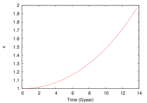
Figure 1: Evolution of the damping parameter $\kappa$ in a $\Lambda$CDM model with $\Omega_{\Lambda}=0.7$, $H_{0}=72km/s/Mpc$

In what follows we will often find it convenient to do our analysis in the time variable $\tau$ and thus consider the equations of motion in the form (6) where $\Gamma$ is related to $\kappa$ by (8). This has the advantage of allowing a simultaneous treatment of the static limit ($\Gamma=0$), and will also be the form we will exploit in our numerical simulations. When necessary or instructive we will change back, for $\kappa\neq 0$, to the more familiar cosmological time variable $t$ or scale factor $a$, noting that the relevant transformations are given by

$$t=t_{0}e^{\kappa\tau/t_{0}}=t_{0}e^{3\Gamma\tau}$$ (10)

and thus

$$a=e^{2\kappa\tau/3t_{0}}=e^{2\Gamma\tau}.$$ (11)

2.1 Collisionless limit

The Vlasov-Poisson limit for our class of models, in the coordinates $(\vec{x},\tau)$ in which the equations of motion are given by (6) with $\Gamma$ constant and ${\bf F}_{i}$ the (regulated) gravitational force, can be written in the simple form

$$\partial_{\tau}f+{\bf v}\cdot\nabla_{\bf x}f-(\nabla_{\bf x}\Phi)\cdot\nabla_{\bf v}f=\Gamma\nabla_{\bf v}\cdot({\bf v}f)$$ (12)

where $f=f(\vec{x},\vec{v},t)$ is the phase space mass density with $\vec{v}=\frac{d\vec{x}}{\delta\tau}$, and

$$\nabla_{\bf x}^{2}\Phi=4\pi G[\int fd^{3}xd^{3}v-\rho_{0}]$$ (13)

2.2 Linear perturbation theory in the collisionless limit

Following the analogous steps to the usual treatment (see Peebles (1980); Binney & Tremaine (1994)) we obtain, by taking moments of these equations and neglecting velocity dispersion, the continuity and Euler equation. Linearizing in the velocity field and density perturbations, and using the Poisson equation (with subtracted mean density), we obtain

$$\frac{d^{2}{\delta}}{d\tau^{2}}+\Gamma\frac{d{\delta}}{d\tau}=4\pi G\rho_{0}\delta$$ (14)

where

$$\delta\left(x,t\right)=\frac{\rho(x,t)-\rho_{0}\left(t\right)}{\rho_{0}\left(t\right)}$$ (15)

is the normalized density fluctuation.

These equations have a decaying and growing mode solution, the latter being given by

$${\delta}\propto D(\tau)=e^{2\alpha\Gamma\tau}\quad{\rm where}\quad\alpha=\frac{1}{4}[-1+\sqrt{1+\frac{24}{\kappa^{2}}}]$$ (16)

For $\kappa\neq 0$ this can be written simply as

$$D(a)=a^{\alpha}$$ (17)

For $\kappa=1$ we thus recover the growth law as in the standard EdS model. Comparatively growth is “slowed down” for $\kappa>1$, and “sped up” for $\kappa<1$. Thus, as would be expected, linear theory retains its scale free nature — characteristic of Newtonian gravity — but it is modified by the addition of damping. Note that in the static limit, $\kappa=0$, we have

$$D(\tau)=e^{\sqrt{4\pi G\rho_{0}}\tau}$$ (18)

We will study (as in almost all cosmological simulations) the case where we start from a time where the theoretical input perturbations are very small and solely in the growing mode. The linear evolution from the same initial conditions in any model in our family can thus be trivially mapped onto that of any other one. To do so it is very convenient to work in the dimensionless time variable $t_{s}(\tau)$ defined by

$$D(\tau)=e^{t_{s}},$$ (19)

i.e.,

$$t_{s}=2\alpha\Gamma\tau={\sqrt{\frac{\pi G\rho_{0}}{6}}}[-\kappa+\sqrt{\kappa^{2}+24}]\,\tau$$ (20)

in which the linear evolution in all models will be identical (in the growing mode). For $\kappa\neq 0$ we have $t_{s}=\alpha\ln a$. We will refer to this time variable as the static time variable, because in the static limit it coincides with the physical time, exactly in “natural” units $\sqrt{4\pi G\rho_{0}}$. Note also that for $\kappa\neq 0$ we have $a=e^{t_{s}/\alpha}$. In our numerical analysis below we will often use this time variable in order to isolate the specific non-trivial dependence of the non-linear clustering on $\kappa$.

2.3 Self-similarity

For a given model with $\kappa$ fixed, self-similarity of the clustering is obtained in principle under precisely the same assumptions as in the usual EdS model Peebles (1980): if (1) the clustering which develops is independent of any length scale other than the single one defined by the non-linearity scale, and (2) the latter scale evolves as predicted by linear theory, the statistical properties should be invariant when expressed in length units which rescale in the same way. Specifically the 2-point auto-correlation function of the density field

$$\xi\left(x\right)=\left<\delta({\bf x^{\prime}})\delta({\bf x^{\prime}}+{\bf x})\right>$$ (21)

should obey the relation

$$\xi(x,\tau)=\xi_{0}\Big{(}\frac{x}{R_{s}(\tau)}\Big{)}$$ (22)

where $\xi_{0}=\xi(x,0)$ and $\tau=0$ is some (arbitrary) reference time. For the power spectrum, which is the Fourier transform of $\xi(x)$, the corresponding relation is

$$P(k,\tau)=R_{s}^{3}(\tau)P_{0}\Big{(}kR_{s}(\tau)\Big{)}\,.$$ (23)

It is commonplace also to define the dimensionless quantity

$$\Delta^{2}(k)=\frac{k^{3}\,P(k)}{2\pi^{2}}\,,$$ (24)

for which the self-similarity relation reads

$$\Delta^{2}(k,\tau)=\Delta_{0}^{2}\Big{(}kR_{s}(\tau)\Big{)}\,\,.$$ (25)

The function $R_{s}(\tau)$ is derived from linear theory, which describes a self-similar evolution from power law initial conditions once the growing mode dominates. Assuming the validity of linear theory at small $k$, so that $P(k,t)\propto D^{2}$, and taking $P(k)\propto k^{n}$, it follows immediately from (23), or equivalently from (22) noting that $\xi(x)\propto 1/x^{n+3}$ at large $x$, that

$$R_{s}=e^{\frac{4\alpha}{3+n}\Gamma\tau}=e^{\frac{2t_{s}}{3+n}}=a^{\frac{2\alpha}{3+n}}$$ (26)

where the last equality holds for $\kappa\neq 0$.

The two central assumptions stated above in deriving this result impose constraints on the range of $n$ for which it can be expected to hold Peebles (1980). For the first condition we require $n>-3$, since if $n\leq-3$ density fluctuations diverge unless an infrared cut-off is imposed (and this cut-off then becomes a relevant length scale). The second condition requires $n\leq 4$ since for $n>4$ linear theory is no longer valid: non-linear evolution produces a $k^{4}$ tail in the power spectrum at small $k$ which will dominate over the initial power.

Whether there are in fact more restrictive bounds on self-similarity has been discussed quite extensively in the literature, and it has been one of the aims of numerical simulation to determine its actual range of validity. Whether the fact that the variance of the velocity fields, proportional in linear theory to that of the gravitational field, requires an infrared regularization for $-3<n<-1$ may lead to breaking of self-similarity has been the subject of some consideration (see Jain & Bertschinger (1996) and references therein). The conclusion of both theoretical and numerical study (for the standard EdS model) is that this is not the case. The essential point is that what is relevant in the clustering dynamics is the difference in gravitational forces on point at a finite separation, and the fluctuations in this quantity have exactly the same infrared properties as those in the mass density field (Jain & Bertschinger (1996), see also discussion in Gabrielli et al. (2010)). Other authors have placed in question the validity of self-similarity at larger $n$, on the grounds that bluer spectra may require ultra-violet regulation of physically relevant quantities. Notably the range $1<n<4$ has sometimes been hypothesized to be excluded, because the mass fluctuation in a top-hat window becomes dependent on the ultraviolet cut-off Peebles (1980), or because the fluctuations in gravitational fluctuations require such a cut-off (see e.g. Smith et al. (2003)). To our knowledge the only numerical study of this range in three dimensions prior to the present one is that of Baertschiger et al. (2007a) for $n=2$ in a static universe, which has found that self-similarity does indeed apply in this case. The one dimensional study of Yano & Gouda (1998) treats the cases $n=1,2,3$ for $\kappa=1$, that of Joyce & Sicard (2011) both $n=2$ and $n=4$ for $\kappa=1$ and $\kappa=\sqrt{3}$, while Benhaiem et al. (2013) treats $n=2$ for many models with $\kappa$ ranging from $0$ to $2$. All find self-similar evolution in these cases. Below we will report results showing clearly that self-similarity is manifestly valid for $n>1$ in three dimensions not only in the usual EdS model, but also in the full family of models we treat.

2.4 The stable clustering approximation for subsystems

The basis of the stable clustering hypothesis in the usual EdS model is the fact that a finite substructure in an expanding universe, provided tidal forces exerted by all other mass may be neglected, evolves in physical coordinates as if it were an isolated self-gravitating system in a non-expanding universe. Formally this can be seen by transforming the equations of motion in the form (1), using (2) with the smoothing set to zero, to physical coordinates ${\bf r}_{i}=a(t)\,{\bf x}_{i}$. This gives

$$\frac{d^{2}{\bf r}_{i}}{dt^{2}}=-Gm\sum_{j\neq i}^{P}\frac{{\bf r}_{i}-{\bf r}_{j}}{|{\bf r}_{i}-{\bf r}_{j}|^{3}}+\frac{1}{a}\frac{d^{2}a}{dt^{2}}\bf{r}_{i}.$$ (27)

The infinite sum on the right hand (with the implicit regularization given by subtracting the mean density) can be calculated by summing in a sphere with centre at the centre of mass of the chosen substructure, and taking its radius to infinity. This sum can then be divided into three parts: (1) the force exerted by the other particles in the substructure, (2) the force exerted by the particles outside the substructure, and (3) the force associated with the subtraction of the background, which by Gauss’ theorem, may be written as $+\frac{4\pi G}{3}\rho_{0}[\bf{r}_{i}-\bf{r}_{c}]$ where $\bf{r}_{c}$ is the position of the centre of the subsystem. Neglecting in the second contribution all but the net force exerted at $\bf{r}_{c}$, using $\frac{1}{a}\frac{d^{2}a}{dt^{2}}=-\frac{4\pi G}{3}\rho_{0}$, and setting ${\bf r}_{c}=0$ (so that ${\bf r}_{i}$ is the position relative to the centre of mass), we obtain for particles in the substructure ${\cal S}$,

$$\frac{d^{2}{\bf r}_{i}}{dt^{2}}=-Gm\sum_{j\neq i,j\in{\cal S}}\frac{{\bf r}_{i}-{\bf r}_{j}}{|{\bf r}_{i}-{\bf r}_{j}|^{3}},$$ (28)

where ${\bf r_{i}}$ is now the position relative to the centre of mass of the subsystem, i.e., the equations of motion of a completely isolated substructure.

For the class of models we are studying the same steps may be followed, the only difference being that we have now $\frac{1}{a}\frac{d^{2}a}{dt^{2}}=-\kappa^{2}\frac{4\pi G}{3}\rho_{0}$ and therefore obtain instead

$$\frac{d^{2}{\bf r}_{i}}{dt^{2}}=-Gm\sum_{j\neq i,j\in S}\frac{{\bf r}_{i}-{\bf r}_{j}}{|{\bf r}_{i}-{\bf r}_{j}|^{3}}+\frac{1}{a^{3}}(1-\kappa^{2})\frac{4\pi G}{3}\rho_{0}\bf{r}_{i},$$ (29)

where ${\bf r}_{i}$ is, again, the position with respect to the centre of mass of the substructure.

Thus, for $\kappa\neq 1$, the equations in physical coordinates for a subsystem, in absence of tidal forces from other mass, include a contribution from the background coming from the component of the comoving mass density $(\kappa^{2}-1)\rho_{0}$ which does not cluster. Note that the result applies also for $\kappa=0$, in which the physical and comoving coordinates are identical, and (29) is then simply a direct rewriting of (1) in which the background subtraction (“Jeans’ swindle”) is explicited (and the tidal forces neglected).

Considering a subsystem of radius $\sim R$ containing $N$ particles, we note that the first force term ${\bf F}_{\cal S}$ is of order $GmN/R^{2}$. If the force term associated with the background is denoted ${\bf F}_{B}$ we then have that

$$\frac{\|{\bf F}_{B}\|}{\|{\bf F}_{\cal S}\|}\sim\frac{|1-\kappa^{2}|}{a^{3}}\frac{\rho_{0}}{\rho_{\cal S}}$$ (30)

where $\rho_{\cal S}$ is the physical mass density of the subsystem. The condition that the subsystem is non-linear is simply that its density be large compared to the mean density, i.e., ${\rho_{\cal S}}\gg\rho_{0}/a^{3}$. Thus, in the same approximation, the background term in the equations of motion in physical coordinates becomes a small perturbation. In absence of this term the substructure will virialize and remain stationary in physical coordinates, i.e., with $\rho_{\cal S}$ approximately constant. Thus for $\kappa>0$ a non-linear system on which the tidal forces of other mass can be neglected, will always asymptotically virialize and remain macroscopically stable in physical coordinates. The smaller is $\kappa$, the longer time (and higher density) will be needed to reach this regime, while in the static limit it may never be better than a reasonable approximation (as the density of the structure relative to the background will not, a priori, grow). In any case, as we will discuss below, the approximation that structures may evolve independently of others in this way is clearly one which will break down for sufficiently small $\kappa$.

2.5 Exponent of non-linear two point correlation function

Let us now make the assumption that, in some range of scale, the statistical properties of the non-linear structure which develop are stable in physical coordinates. Assuming that the associated clustering is self-similar, this implies immediately that the clustering in this range is strictly scale-free in our models, i.e., it has no characteristic length scale: if there were such a scale it would scale in time in comoving units in proportion to $1/a$, which is inconsistent with the self-similar form of the two point correlation function (22). In short: if there is a regime of self-similar stable clustering in these models, it must be truly scale-free. As underlined in Peebles (1980), this implies that the associated clustering is fractal in nature, corresponding to a “virialized hierarchical” clustering.

Such clustering is characterized by its exponents, and we focus here just on the two point correlation function. If there is a regime of stable clustering, it must then have a power law behaviour $\xi(x)\sim x^{-\gamma_{sc}}$. To derive this exponent it suffices to consider that it applies at any time between two scales: a scale $x_{min}$ and $x_{max}$ say. The upper cut-off, marking the breakdown of stable clustering, must scale as required by self-similarity, i.e., $x_{max}\propto R_{s}(\tau)$, and correspond to some constant value $\xi(x_{max})=\xi_{max}$. The lower cut-off $x_{min}$, on the other hand, must scale in the same way only if the clustering is self-similar below this scale. Alternatively this lower cut-off $x_{min}$ can scale differently, and in this case it marks also a lower cut-off to self-similarity. In this case $x_{min}$ is necessarily related to some other scale in the system, such as the initial interparticle distance, or the force smoothing length. As we will discuss, this appears to be the case actually realized in all our numerical simulations (which have finite resolution).

To calculate the exponent associated with stable clustering, we consider the correlation function between an arbitrary physical scale $r_{sc}$ in the range of stable clustering, and the scale $x_{max}$. In comoving units the former corresponds to a scale which depends on time as $x_{sc}(\tau)=x_{sc}(0)a_{0}/a$. In the non-linear regime, $\xi\gg 1$, and stability of clustering in physical coordinates implies that $\xi$ varies only because of its normalisation to the mean density in physical coordinates, i.e., $\xi(x_{sc}(\tau))=\xi(x_{sc}(0))(a/a_{0})^{3}$. Assuming a power law behaviour of the correlation function, $\xi(x)\sim x^{-\gamma_{sc}}$, and using these scalings, we have

$$\gamma_{sc}=-\frac{{\ln\left(\frac{{{\xi_{max}}}}{{{\xi_{sc}}}}\right)}}{{\ln\left(\frac{{{x_{max}}}}{{{x_{sc}}}}\right)}}=\frac{3{\ln\left(\frac{a}{a_{0}}\right)}+{\ln\left(\frac{{{\xi_{sc}(a_{0})}}}{{{\xi_{max}}}}\right)}}{\left(\frac{2\alpha}{3+n}+1\right){\ln\left(\frac{a}{a_{0}}\right)}+{\ln\left(\frac{{{x_{max}(a_{0})}}}{{{x_{sc}(a_{0})}}}\right)}}\,.$$ (31)

We can always choose $a_{0}$ such that $x_{max}=x_{sc}(a_{0})$, at which time $\xi_{sc}(a_{0})=\xi_{max}$, and therefore we have

$$\gamma_{\rm sc}\left({n,\kappa}\right)=\frac{3(3+n)}{3+n+2\alpha}=\frac{6(3+n)}{5+\sqrt{1+\frac{24}{\kappa^{2}}}+2n}\,.$$ (32)

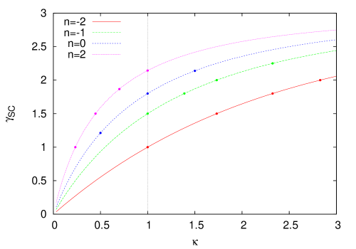
Figure 2: Exponent $\gamma_{sc}$ of the non-linear two point correlation function predicted using the stable clustering hypothesis, as a function of $\kappa$ for different chosen $n$. The usual EdS prediction corresponds to the case $\kappa=1$. The points on the solid line indicate the models for which we report results of numerical simulations in the second part of the paper.

This result is plotted in Fig. 2 showing the prediction $\gamma_{\rm sc}\left({n,\kappa}\right)$ as a function of $\kappa$ for different $n$. In the case $\kappa=1$ we recover, as expected, the well known result of Davis & Peebles (1977); Peebles (1980) :

$$\gamma_{\rm sc}\left({n,\kappa=1}\right)=\frac{3(3+n)}{5+n}\,.$$ (33)

Note that $\gamma_{\rm sc}\left({n,\kappa}\right)$ is positive provided $n>-3$, which is, as we have discussed above, precisely the lower bound on $n$ for which self-similarity can apply. Further $\gamma_{\rm sc}\left({n,\kappa}\right)$ is a monotonically increasing function of both $\kappa$ and $n$, and it is bounded above by the spatial dimension. This is precisely the bound which is required if the correlation function is that of a scale invariant mass distribution (as $3-\gamma$ is the associated fractal dimension). For $\kappa=0$ on the other hand, we obtain $\gamma_{\rm sc}=0$. This means that in this limit the predicted exponent is not consistent with a scale invariant distribution, and indeed, as we will discuss further below, the stable clustering hypothesis ceases to be physically reasonable in this case.

2.6 Validity of stable clustering

Let us now consider the validity of the stable clustering hypothesis. In models of the kind we study, with cold initial conditions, and with $n$ in the range $-3<n\leq 4$, structure formation is hierarchical in nature: fluctuations go non-linear and collapse at successively larger scales. In the stable clustering hypothesis we suppose that structures collapse and virialize at a given time and are thereafter essentially undisturbed by the subsequent evolution, i.e., they are subsumed in larger structures but remain essentially unchanged in physical coordinates (with respect to their own centre of mass). Clearly this can be at best a good approximation for some time: any given structure will evolve in physical coordinates because of interactions with other structures, and indeed can even merge with other ones. The relevant question is therefore how good an approximation stable clustering provides, rather than whether the stable clustering hypothesis is strictly valid or not. More specifically the question is how well the predictions for macroscopic quantities furnished by this hypothesis work, and over what range of scale. In the second part of this paper we will focus, as in various other works in the literature, on trying to answer this question for the two point correlation function in the non-linear regime, for which we have just derived the prediction.

The class of models we are studying is a two dimensional family, and, if stable clustering is a relevant approximation for describing non-linear clustering, we would expect that the degree to which it is valid will depend on the parameters $\kappa$ and $n$. In the preceeding study Joyce & Sicard (2011); Benhaiem et al. (2013) of models in one spatial dimension, we have shown that there is in fact a simple qualitative answer to this question which is suggested by simple theoretical considerations, and which turns out to be remarkably well born out by numerical study. With trivial modifications, as we will now explain, the same considerations apply in three dimensions: assuming stable clustering (and self-similarity) to apply, the exponent $\gamma_{sc}$ we have just calculated can be shown to control directly the relative size of virialized objects of different masses; it is natural, as we will explain, to consider this as probably the essential parameter controlling the validity of stable clustering. More specifically, this reasoning suggests that the criterion for the validity of stable clustering can be expected to be that $\gamma_{sc}$ be sufficiently large. This expectation has been born out in the one dimensional models, with the “critical value” situated at $\gamma_{sc}\approx 0.15$. The goal of our numerical study in this paper is to see if an analogous result holds in three dimensions.

Let us consider then two overdensities of mass $M_{1}$ and $M_{2}>M_{1}$, corresponding to initial comoving scales $L_{1}^{0}$ and $L_{2}^{0}$ respectively. Assuming that their collapse is self-similar (as, for example, in the spherical collapse model), the ratio of their sizes when they virialize is equal to the initial value of this ratio. One can infer also that the time-delay between their respective virialization, at scale factors $a_{1}$ and $a_{2}$ say, is given by

$$R_{s}(\tau_{2}-\tau_{1})=\left(\frac{a_{2}}{a_{1}}\right)^{\frac{2\alpha}{3+n}}=\left(\frac{L_{2}^{0}}{L_{1}^{0}}\right)$$ (34)

Now, if we assume that the first structure is stable from the time it virializes, we can deduce that the ratio of the sizes of the two structures decrease by a factor of $\frac{a_{1}}{a_{2}}$ during the interval between their virialization. Thus, when the second (larger) structure virializes, we have that the ratio of the sizes of the two structures is

$$\frac{(L_{2}/L_{1})}{(L_{2}^{0}/L_{1}^{0})}=\left(\frac{L_{2}^{0}}{L_{1}^{0}}\right)^{-\frac{3+n}{2\alpha}}=\left(\frac{L_{2}^{0}}{L_{1}^{0}}\right)^{-\frac{\gamma_{sc}}{3-\gamma_{sc}}}$$ (35)

Quite simply, the larger is $\gamma_{sc}$, the more a structure which has virialized can “shrink” relative to a larger structure which virializes later. Or, in other words, the larger $\gamma_{sc}$ is, the more “concentrated” are the pre-existing virialized substructures inside a larger structure when it collapses. This is precisely the property one would expect to be relevant for the validity of stable clustering: if the sub-structures inside a structure are smaller (and therefore more tightly bound), the process of their disruption by tidal forces and mergers will be much slower and less efficient. Indeed, in the limit that $\gamma_{\rm sc}$ tends to its upper limit, any structure which collapses and virializes will see the substructures which have collapsed before it essentially as point particles, and thus stable clustering should become exact in this limit. As $\gamma_{\rm sc}$ decreases, on the other hand, we expect that the interaction between structures can lead more easily to their disruption, and in particular that mergers of substructures become much more probable.

More precisely we would expect that, in a given scale-free model (i.e. for given $n$ and $\kappa$), there will be a time scale $\tau_{s}$ characteristic of the stability of any structure. Now if self-similarity applies, i.e., if no other length scales (particle discreteness scale, force smoothing scale) have any influence on the macroscopic evolution of the structure, this time scale should be the same, for any structure, when expressed in terms of its own dynamical time scale. This means that if a structure virializes at scale factor $a_{v}$, its stability will remain a good approximation until some scale factor $a_{s}$ where the ratio $a_{v}/a_{s}$ has some fixed value, $\eta_{s}$ say. Supposing this to be the case leaves the derivation given above of the exponent $\gamma_{sc}$ unchanged — no assumption about the behaviour of the lower cut-off to stable clustering was made. However it gives us also a prediction that the power law region in the correlation function should have a lower cut-off $x_{min}\sim\eta_{s}x_{max}$. Adopting the arguments above, we would expect this ratio $\eta_{s}$ to depend on $n$ and $\kappa$ only through $\gamma_{\rm sc}$, and to decrease monotonically as $\gamma_{\rm sc}$ increases, so that the range of scale in which stable clustering may apply will stretch monotonically as $\gamma_{\rm sc}$ increases. Note that, in any case, the scale $x_{min}$, if it exists, must then also scale as defined by self-similarity, i.e., $x_{min}\propto R_{s}(\tau)$.

2.7 Range of stable clustering in a finite simulation

The above considerations, and the evidence supporting them in the one dimensional studies of Joyce & Sicard (2011); Benhaiem et al. (2013), motivate and structure our numerical study: the goal is to measure, in our $(n,\kappa)$ model space, as well as possible the form of the self-similar two point correlation function and to determine in particular in what range of scale the prediction of stable clustering may describe it well. In particular we would like to determine, whether, as anticipated, $\gamma_{sc}(n,\kappa)$ is the parameter relevant to answering this question, and if there a characteristic or “critical” value of $\gamma_{sc}(n,\kappa)$ below which the stable clustering approximation breaks down completely, as has been found in the one dimensional studies (at a value $\gamma_{sc}$ in the range between $0.15-0.2$). These studies also illustrate the numerical difficulties which arise in addressing these questions, and the extent to which they can actually be understood and anticipated from the considerations above. Indeed, as we will now explain, we expect $\gamma_{sc}$ not only to be an indicator for the range of scales in which the “true” self-similar two point correlation function —- without any limit of spatial resolution — may be well described by the stable clustering predictions, but also to control the range of scale over which it may potentially be measured in a numerical simulation of a given finite size.

Given that we set out to detect self-similar clustering, and to assess the validity in particular of the stable clustering approximation, it is evidently relevant to estimate the range of scales over which such self-similar stable clustering would be expected to develop in a simulation of given particle number $N$, if we assume that this approximation apply. The particle number $N$ fixes the simply the temporal range over which evolution can be simulated, as this is bounded above by the time at which the scale of non-linearity approaches the box size. Let us call $\tau_{i}$, corresponding to $a=a_{i}$, the time when the first non-linear structure — say of order one hundred particles — virializes, with a comoving size $x_{i}$. The simulation can be run (if numerically feasible) until a time $a=a_{f}$ when the largest approximately virialized region is of a size $x_{f}$reaches some small fraction of the box-size $L$. Using self-similarity it follows that

$$\left(\frac{a_{f}}{a_{i}}\right)^{\frac{2\alpha}{3+n}}\approx\left(\frac{x_{f}}{x_{i}}\right)$$ (36)

Assuming further that structures are stable once they virialize we have that $x_{min}(a_{f})$, the lower cut-off to stable clustering the end of the simulation, obeys the relation

$$\ln\left(\frac{x_{min}(a_{f})}{x_{i}}\right)\approx\ln\left(\frac{a_{i}}{a_{f}}\right)\approx\frac{\gamma_{sc}}{3-\gamma_{sc}}\ln\left(\frac{x_{f}}{x_{i}}\right)\,.$$ (37)

Likewise, using again that the upper cut-off to stable clustering $x_{max}$ at the final time is simply $x_{f}$, we have

$$\ln\left(\frac{x_{min}(a_{f})}{x_{max}(a_{f})}\right)\approx\frac{3}{3-\gamma_{sc}}\ln\left(\frac{x_{f}}{x_{i}}\right)$$ (38)

These estimates can be modified easily to incorporate a breakdown of stable clustering as discussed above. This becomes relevant if it is possible to evolve sufficiently long so that $a_{i}/a_{f}<\eta_{s}$, in which case the scale $x_{min}(a_{f})$ can then becomes smaller than the “true” $x_{min}$, and this lower cut can in principle be resolved.

For a simulation of given size, the ratio $\frac{x_{f}}{x_{i}}$ is, to a first rough approximation, independent of both $n$ and $\kappa$: $x_{i}$ is proportional to the initial interparticle distance, and $x_{f}$ is limited to be some fraction of the box size. Therefore, if stable clustering applies, it will become increasingly difficult to robustly probe it numerically as $\gamma_{sc}$ decreases. In short just as the range $[x_{min},x_{max}]$ is expected to shrink as $\gamma_{sc}$ decreases, the range of numerically accessible scales does too. Conversely, to access as much of the range over which we can measure the exponents for larger $\gamma_{sc}$, we will need to use a small force smoothing (to resolve down to $x_{min}(a_{f})$) which is more challenging numerically.

3 Numerical simulations: methods and results

The aim of our study here is to characterize how non-linear clustering depends on the initial conditions, parametrized by $n$, and the cosmology, parametrized by $\kappa$. We have thus aimed to produce a large library of $N$ body simulations (of purely self-gravitating “dark matter” particles) covering a significant range of these parameters. In this paper we will focus our analysis on two point correlation properties, while other complementary analyses using other tools will be reported in future work. In particular, as discussed, we will focus here on the degree of validity of self-similarity and the relevance of the stable clustering approximation.

3.1 Simulation Code

To do our simulations we have chosen to use the widely used and very versatile GADGET2 code (Springel, 2005). As the class of models we have described are not equivalent to those which can be simulated by the code — models specified by the standard cosmological parameters — we need to modify it appropriately in order to realize this possibility. To do so one possibility is to modify the cosmological version of the code. Another one, which is the method we have chosen, is to modify the static universe version of the code (i.e. non-expanding system in periodic boundary conditions) exploiting the fact, which we have highlighted, that in our models the equations of motion may be written in the form (6) where $\Gamma$ is a constant, i.e., the system is equivalent to a static universe with a constant fluid damping. We have thus modified the time-integration scheme of GADGET2 keeping the original “Kick-Drift-Kick” structure of leap-frog algorithm and modifying appropriately the “Kick” and “Drift” operation. The structure of the code is otherwise unchanged. Details can be found in Appendix  A.

Tests of this code — notably using energy conservation — will be discussed below in assessing the reliability of the results of all our simulations. One additional simple independent test of it we have done is the following: comparison between the case $\kappa=1$, which corresponds to the usual EdS model, with the results obtained for this case using the cosmological — expanding universe — version of GADGET2 for the same case (i.e. $\Omega_{m}=1$ and $\Omega_{\Lambda}=0$). We have performed this test and found very satisfactory results. Shown, for example, in Fig 3, is the comparison of the results obtained using the two codes, evolved up the same scale factor, starting from an identical initial condition given by a realization of the case $n=0$. [Further details on the numerical parameters chosen will be given below, and we note that we use here, as everywhere in the paper, length units in which the periodic box size is unity]. The left panel shows a projection of the particle positions, with those corresponding to the “standard” code in red and those of our modified static code in green; the right panel shows the two point correlation function measured in the two cases, with the black vertical line indicating the force smoothing scale. While the first reveals some visual differences between the two simulations — which is to be expected as these are two different integrations of the same chaotic system — the latter shows that the statistical properties (which is what we will measure with such simulations) are in almost perfect agreement.

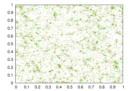
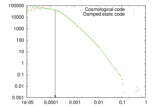
Figure 3: Comparison of results obtained from two EdS ($\kappa=1$) simulations of identical $n=0$ initial conditions: in the left panel, the particle positions in the simulation box projected onto a plane; in the right panel, the measured two point correlation functions. The green points correspond to a simulation performed using our modification of the static version of GADGET2, and the red points a simulation using the existing cosmological version of the code.

3.2 Simulation parameters

Our results reported here are based on simulations from power law initial conditions with exponents taking the values $n=-2,-1,0,2$ and values of $\kappa$ ranging in the $\kappa=0.23$ to close to $\kappa=3$. Table 1 gives the exact values of $n$ and $\kappa$, and in each case also the associated predicted stable clustering exponent $\gamma_{sc}$, as well as other parameters characterizing the initial amplitude and duration of the simulation which we will discuss below. As discussed in detail below this prediction turns out to be very good, and likewise, the estimates which we have given above for the range over which non-linear clustering develops. The choices of the values of $\kappa$ simulated at each $n$ are thus appropriately guided by the associated value of $\gamma_{sc}$, which we have chosen to vary in the range $1\leq\gamma_{sc}\leq 2.25$. The simulations in Table 1 are for $N=128^{3}$ particles for the cases $n=-2$, and for $N=64^{3}$ otherwise. We report separately at the end of this section a comparison with a pair of larger simulations with $N=256^{3}$ for one case ($n=-1$, $\kappa=1$).

The lower bound on the range of $\gamma_{sc}$ has been chosen because, at $\gamma_{sc}\sim 1$ (corresponding to $n=-2$ for the case $\kappa=1$), we find that the region of self-similarity we can access becomes too small to allow any robust statement about the strongly non-linear part of the correlation function. As we will discuss below, this is a simple generalisation of the same difficulty which has been observed in the literature for the usual $\kappa=1$ case, where the accessible range of self-similarity has indeed been observed to decrease greatly as $n$ decreases towards $-3$, with the validity of self-similarity below $n=-1$ a subject of discussion in the literature (Efstathiou et al., 1988; Jain & Bertschinger, 1996, 1998). As we will highlight below, one of the things we show very clearly from our study in this larger class of models is that this difficulty is not essentially related to the convergence properties in the infra-red of these spectra, but instead arises because $\gamma_{sc}$ is small. Indeed at $n=-2$ we will see that we have no difficulty observing self-similarity when $\kappa$ is increased significantly above unity.

The upper bound on $\gamma_{sc}$ is, on the other hand, related to the lower limit on the spatial resolution imposed by the force smoothing. We use the version of GADGET2 with a smoothing which is fixed in comoving coordinates (as is the practice in many large volume cosmological simulations, and in particular in almost all studies of the issues explored here). The choice of the force smoothing parameter $\varepsilon$ is an essential question as it conditions also greatly the number of particles which can be simulated, for given numerical resources: smaller smoothing requires smaller time steps. In order to determine whether stable clustering applies, however, we must clearly have the numerical resolution necessary to detect it if it is a good approximation, and this imposes in principle the choice of an $\varepsilon$ which is as small as possible. To do so, we need to be able to “follow” for as long as possible the (possibly stable) evolution of non-linear structures. The first virialized structures which can be resolved — with of order one hundred particles, say — have a size of order the initial interparticle distance $\Lambda=L/N^{1/3}$. For $\kappa=1$, for example, the density at virialization — following the standard estimate of the spherical collapse model — is of order $200$ times the mean mass density, equal to $1/\Lambda^{3}$. Such a structure can only be well simulated provided the force smoothing, $\varepsilon$, is sufficiently small compared to the size of the structure. In the case of stable clustering its size decreases in comoving coordinates, in proportion to $1/a$. Thus, for chosen $f=\varepsilon/\Lambda$, we can follow the (possible) stability of structures over a range of scale factor strictly bounded below by $1/f$. This can be seen also in terms of the estimate (37) given above: in order to resolve fully the regime of stable clustering we need $\varepsilon$ to be significantly smaller than $x_{min}$. It is clear that, if stable clustering applies and we wish to resolve it well for values of $\gamma_{sc}\sim 2$, we need to have a value of $\varepsilon$ very considerably smaller than $\Lambda$. We could, alternatively, evolve the system to times when structures containing a significant number of particles should, following stable clustering, “shrink” below the smoothing scale. In principle one should still obtain then the correct evolution sufficiently far above $\varepsilon$. However the scale and manner in which clustering above $\varepsilon$ is modified in such a regime is very difficult to control for and would introduce another source of uncertainty in our results.

Given these considerations, and following tests of the numerical cost of simulations, and of energy conservation (see below), we have thus chosen to take the following values for the GADGET2 parameters in the simulations reported in Table 1:

• Force softening $\varepsilon=0.01\Lambda$ (corresponding to a spline softening with compact support of radius $2.8\,\varepsilon$)

• Timestepping parameters: ErrTolIntAccuracy=0.001, MaxRMSDisplacementFac=0.1 and MaxSizeTimestep=0.01. We note that these values are smaller (by factors of $25$ for the first, and $2.5$ for the two others) than the values suggested in the GADGET2 userguide and treated as “fiducial” in the literature (see e.g. Smith et al. (2012)). These choices were made as we found they gave significant improvement in energy conservation (see discussion below).

• Force accuracy fixed by ErrTolForceAcc=0.005 (a typical fiducial value)

In the final section of the paper we will compare in detail our results to the previous studies (of EdS models), in particular to those of Smith et al. (2003) and Jain & Bertschinger (1998). We just note here that the most important point to remark in our parameter choice is that our force smoothing, in units of the initial grid spacing $\Lambda$, is approximately the same as that of Jain & Bertschinger (1998), but about six time smaller than that of Smith et al. (2003). On the other hand, the particle numbers ($N=128^{3}$ for our $n=-2$ simulations and $N=64^{3}$ for the others) are smaller than those of both these other studies ($N=256^{3}$). Thus, while we have considerably better resolution of non-linear clustering at small scales than Smith et al. (2003) — and in particular, as we will see, we can follow fully the propagation of self-similarity to smaller scales — our results may be more subject to finite size effects coming from the periodic box. While self-similarity provides in principle a good test for both potential biases associated with the use of a small smoothing parameter and with finite box size effects, we will also test carefully below more directly for both effects using, for a few chosen cases, additional simulations with both larger smoothing and larger particle number. In particular we will report at the end of the section a comparison of our results with a pair of further simulations with $N=256^{3}$ particles for one chosen model ($n=-1$ and $\kappa=1$). For what concerns the use of a relatively small force smoothing, one possible issue is possible bias of the desired mean-field evolution due to two body collisionality. In practice the main associated difficulty (see e.g. Knebe et al. (2000); Joyce & Labini (2013)) is that small smoothing can leads to poor energy conservation if the numerical accuracy of the integration of hard collisions is not sufficiently accurate. With this particular concern in mind, we have performed, as reported in detail below, detailed tests of energy conservation, and have adapted tight criteria leading to the very accurate choice of time-stepping parameters given above. If, on the other hand, two body collisions are integrated correctly, the associated effects will not be diagnosed by an analysis of energy. However, if in such a case such collisions actually modify the macroscopic evolution, we should observe a breaking of self-similarity induced by this. Thus such effects, if they are present, should also be excluded from our analysis by the test of self-similarity (which we will apply to all our results).

Our simulations were executed using a cluster at the University of Nice using MPI on between 32 and 128 processors, depending on the simulation. The time necessary to run them varied from a few days to a few weeks.

n	$\kappa$	$\gamma_{sc}$	$\Delta^{2}_{L}(k_{N},t_{s}^{0})$	$t_{s}^{f}$	$\Delta^{2}_{L}(k_{b},t_{s}^{f})$
-2	1.00	1.00	0.03	3.00	1.96 $\times 10^{-1}$
-2	1.73	1.50	0.03	3.00	1.96 $\times 10^{-1}$
-2	2.32	1.80	0.03	2.80	1.31 $\times 10^{-1}$
-2	2.83	2.00	0.03	2.50	7.20 $\times 10^{-2}$
-1	1.00	1.50	0.06	4.00	1.79 $\times 10^{-1}$
-1	1.39	1.80	0.06	4.00	1.79 $\times 10^{-1}$
-1	1.73	2.00	0.06	4.00	1.79 $\times 10^{-1}$
-1	2.32	2.25	0.06	4.00	1.79 $\times 10^{-1}$
0	0.50	1.21	0.94	4.00	8.57 $\times 10^{-2}$
0	1.00	1.80	0.94	4.00	8.57 $\times 10^{-2}$
0	1.50	2.14	0.94	4.00	8.57 $\times 10^{-2}$
2	0.23	1.00	0.94	4.50	2.28 $\times 10^{-4}$
2	0.45	1.50	0.94	4.50	2.28 $\times 10^{-4}$
2	0.70	1.87	0.94	6.00	4.57 $\times 10^{-3}$
2	1.00	2.14	0.94	5.00	6.19 $\times 10^{-4}$

Table 1: Parameters characterizing our $N$ body simulations with $N=128^{3}$ particles for the cases $n=-2$, and $N=64^{3}$ for the other cases. $t_{s}^{f}$ is the duration in “static time” units of the simulation, equal to the logarithm of the linear growth factor; the quantities $\Delta^{2}_{L}(k_{N},t_{s}=0)$ and $\Delta^{2}_{L}(k_{b},t_{s}^{f})$ characterize the initial and final amplitudes of the fluctuations. Note that we use units in which the box size is unity so that the wavenumber $k_{b}$ of the fundamental mode $k_{b}$ is equal to $2\pi$.

3.3 Initial conditions and duration of simulations

We generate our initial conditions using the standard method used in cosmological simulations(see e.g. Bertschinger (1995); Joyce & Marcos (2007)): to particles initially on a simple cubic lattice, we apply a displacement field generated as a sum of independent gaussian variables in reciprocal space with variance determined by the desired linear power spectrum, and including all modes up to the Nyquist frequency $k_{N}=\pi/\Lambda$ (i.e. we sum over $\vec{k}$ such that each component $k_{i}\in[-k_{N},k_{N}]$.) If we denote $\vec{u}_{i,0}$ the resulting displacements of the particles, the initial velocities $\vec{v}_{i,0}$ are then fixed simply using the Zeldo’vich approximation

$$\vec{u}(\tau)=D(\tau)\vec{u}_{i,0}$$ (39)

where $D(\tau)$ is the linear growth factor of the growing mode solution (16) and the simulations starts at $\tau=0$ (and thus $t_{s}=0$) so that

$$\vec{v}_{i,0}=2\alpha\Gamma\,\vec{u}_{i,0}={\sqrt{\frac{\pi G\rho_{0}}{6}}}[-\kappa+\sqrt{\kappa^{2}+24}]\,\vec{u}_{i,0}\,.$$ (40)

We take an initial power spectrum $P_{L}(k,t_{s}=0)=A_{0}k^{n}$, and following common practice we characterize the initial amplitude of fluctuations by specifying the value of $\Delta_{L}^{2}(k_{N})=\frac{A_{0}k_{N}^{3+n}}{2\pi^{2}}$, which is (approximately) the normalized mass variance in a gaussian sphere of radius $\Lambda$. In fixing the initial amplitude of our simulations as given in Table 1, we have used as guidance the previous work notably of Jain & Bertschinger (1998) and Knollmann et al. (2008) which report tests showing that self-similarity is recovered better for the cases of smaller $n$ if low amplitudes are used. Thus the amplitude for our simulations with $n=0$ and $n=2$ corresponds at the starting time to $\Delta^{2}(k_{N})\approx 1$, while for the two other cases they are significantly smaller. Also given in Table 1 are the final times $t_{s}^{f}$ considered for our analysis in each of the simulations, and the corresponding values of the linear theory extrapolated amplitude $\Delta_{L}^{2}(k_{b},t_{s}^{f})$ at the fundamental mode of the periodic box $k_{b}=2\pi/L$. The latter corresponds approximately to the normalized mass variance in a gaussian sphere of order the size of the box. In the cases $n=-2$ and $n=-1$ our simulations thus extend to times when this quantity is no longer much smaller than unity, and one would expect this to lead to significant finite size effects. We will indeed detect such effects clearly and consider carefully the limitations they place on our results. The final times $t_{s}^{f}$ in the other simulations are, on the other hand, significantly smaller than those at which such effects might be expected to become significant, and they are determined in most cases rather by the numerical cost of integration or considerations of energy conservation which we discuss below.

3.4 Monitoring of Energy

In $N$ body simulations in a non-expanding space energy conservation is the most fundamental control on numerical precision, and poor energy conservation (less than a few percent) is known to be indicative typically of a poor representation of macroscopic properties (see e.g. Hockney & Eastwood (1999)). In simulations in an expanding background total energy is not conserved, and one thus no longer disposes of this robust and simple instrument of control on simulation accuracy. Nevertheless one can exploit and test a constraint on the evolution of energy, given by the so-called Layzer-Irvine equation, which is usually written (see e.g; Peebles (1980)) as

$$\frac{dE_{p}}{da}=-\frac{2K_{p}+U_{p}}{a}\,.$$ (41)

where $K_{p}=\frac{1}{2}\sum_{i}ma^{2}(\frac{d{\bf x}_{i}}{dt})^{2}$ is the peculiar or “physical” kinetic energy, $U_{p}$ is gravitational potential energy in physical coordinates and $E_{p}=K_{p}+U_{p}$.

With the equations of motion written in the time variable $\tau$, as in (6), it is very trivial by integration to derive this equation in the form

$$\frac{dE}{d\tau}=-2\Gamma K$$ (42)

where $E=K+U$, and $K=\frac{1}{2}\sum_{i}m\left(\frac{d{\bf x}_{i}}{d\tau}\right)^{2}$ and $U=\frac{1}{2}\sum_{i,j}\phi(|{\bf x}_{i}-{\bf x}_{j}|)$ where $\phi(|{\bf x}|)$ is the two body potential from which the force $\bf F_{i}$ is derived. Note that to derive this relation we need only assume that the two body potential is time independent (in comoving coordinates), so it remains valid including the force smoothing (which is fixed in these coordinates in our simulations). Now, using (5), and thus $K=aK_{p}$ and $U=aU_{p}$, we see that (42) and (41) are equivalent.

Given the equation in the form (42), a natural definition for a parameter to characterize the precision of the numerical evolution of the energy evolution is

$$A_{0}(\tau)=\frac{E(\tau)+2\Gamma\int_{0}^{\tau}Kd\tau}{E_{0}}=\frac{E(a)+\int_{1}^{a}\frac{K}{a}da}{E_{0}}$$ (43)

where $E_{0}=E(\tau=0)$ is the initial energy, and the last equality holds for any $\Gamma\neq 0$. While this parameter clearly reduces to the usual monitoring of energy conservation in the static limit, the choice is clearly not unique, nor necessarily optimal, when we consider an expanding background. Indeed, starting from (41), one might instead take

$$A_{1}(a)=\frac{E_{p}+\int_{1}^{a}\frac{2K_{p}+U_{p}}{a}da}{E_{0}}\,.$$ (44)

Even more generally, for any $\Gamma\neq 0$, and defining $E_{\beta}=E/a^{\beta}$, $K_{\beta}=K/a^{\beta}$, $U_{\beta}=U/a^{\beta}$ the equation (42) can be written as

$$\frac{dE_{\beta}}{da}=-\frac{\beta}{a}E_{\beta}-\frac{1}{a}K_{\beta}\,.$$ (45)

with an associated family of possible parameters

$$A_{\beta}(a)=\frac{\frac{E}{a^{\beta}}+\int_{1}^{a}\frac{\beta E+K}{a^{\beta+1}}da}{E_{0}}\,.$$ (46)

While all of these parameters are equal to unity when (42) is valid, their deviations from unity in a numerical integration are not trivially related to one another and it is not a priori clear which, if any of them, provides the most suitable measure of the accuracy of a simulation. The problem with this kind of measure is that we do not dispose (at least currently) of any absolute calibration which tells us how much deviation from unity of such indicators can be tolerated. In short, while in a non-expanding simulation we know we should tolerate only percent level deviations of the energy, we do not know what deviation from unity of the parameters $A_{\beta}$ should be considered acceptable. Most studies in the cosmological literature which report results for monitoring of the energy evolution (see e.g. Couchman et al. (1995), Pen (1998)), Smith et al. (2003)) consider the parameter

$$A^{\prime}=\frac{E_{p}(a)-E_{0}+\int_{1}^{a}\frac{2K_{p}+U_{p}}{a}da}{U_{p}}\equiv\frac{E_{0}}{U_{1}}(A_{1}-1)\,,$$ (47)

i.e., the integrated fluctuation is normalized with the physical potential energy $U_{p}$ rather than the initial total energy. While in absence of any absolute calibration for any of these parameters, one cannot know which parameter is the most appropriate to use, it appears to us, compared to the parameter $A_{1}$, that this canonical normalisation is probably not an astute one. Firstly, extrapolated to the non-expanding limit by taking $\Gamma\rightarrow 0$, it corresponds to normalizing the total energy fluctuation to an energy which evolves, and typically increases in magnitude in time, due to the development of clustering. Thus one can obtain arbitrary variation (and typically decrease) in the measured “energy error” measured with $A^{\prime}$ which would appear to have a priori little to do with (integrated) numerical error. Further we have found, tracing its behaviour, that $A^{\prime}$ can even diverge because the potential energy can change sign (as it may be positive in the almost uniform initial configuration).

The crucial point is that, in any case, with the current absence of any absolute calibration, we can use these parameters only as a tool to compare the accuracy of different simulations, but not to make any useful inference about their absolute accuracy. In the course of this study we have, in our choice both of numerical simulation parameters and the range of $n$ and $\kappa$ simulated, made use of both $A_{0}$ and $A_{1}$, in this way. In particular, as mentioned above we found in test simulations that their difference from unity could be reduced significantly taking the time step parameters we have chosen, compared to fiducial values. Further, and more interestingly, we have found that large deviations from unity of these parameters are often clearly correlated with a breakdown of self-similarity. This opens up the possibility of using this class of models as an absolute calibrator for accuracy of numerical simulations as probed by parameters like $A_{\beta}$. These issues will be discussed at length elsewhere. We report here, for brevity, only measurements with the indicator $A_{1}$, because it is the one closest to the often used $A^{\prime}$. Further it has the nice feature that, for the case of a single isolated virialized structure (for which $2K_{p}+U_{p}=0$, if the effects of force smoothing are negligible), it reduces to the fractional energy error in the physical energy $E_{p}$, which is the error measurement one would usually use for this case.

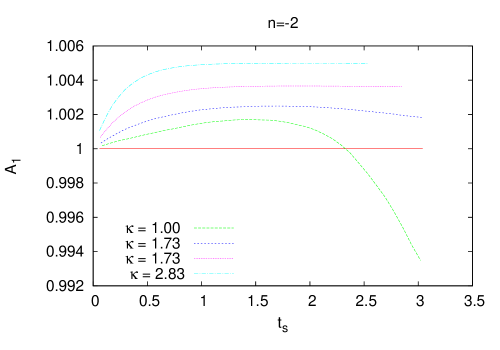
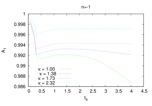
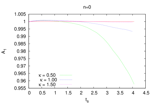
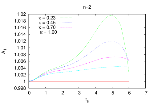
Figure 4: Evolution of the energy evolution parameter $A_{1}$ defined in the text as a function of $t_{s}$.

Shown in Fig. 4 is the evolution of the parameter $A_{1}$ in our different simulations, each panel showing the simulations of a given $n$ for the different $\kappa$. For the case $n=2$ we plot data in all models up to $t_{s}=6$, which for three models is beyond the final $t_{s}^{f}$ given in Table 1, i.e., we include (for the purposes of illustration) some simulation data which we have excluded from our analysis. From Fig. 4 we see that according to this measure the accuracy of the simulations varies, but is of comparable order, with maximal deviations from unity of order at most a few percent. The slightly smaller amplitude of deviations in the case $n=-2$ are a reflection of the larger particle number compared to that in the other cases. For each $n$, we see also that the poorest precision in $A_{1}$ is obtained for the model with the smallest $\kappa$. The model $(n=0,\kappa=0.5)$ shows a significantly larger amplitude deviation from unity than any other, while the models with $n=2$ and smaller $\kappa$ show the onset of a more rapid evolution of $A_{1}$ after reaching a peak. We have excluded from our analysis the later time data in these models precisely because we have concluded that this behaviour is correlated with an unphysical evolution of macroscopic quantities, and specifically a breakdown of self-similarity (which, as we will see, holds at earlier times). To illustrate this a little more, we retain here in our analysis the later time data in the model $(n=0,\kappa=0.5)$ which, we will see, also manifests such a deviation from self-similarity which we believe is a result of the poorer numerical precision indicated by the behaviour of $A_{1}$.

3.5 Effects of force smoothing

As the limitation on the spatial resolution associated with force smoothing is an important issue in interpreting the results of simulations, we have performed some studies of the effect of varying $\varepsilon$. Shown in Fig. 5 are results for the correlation functions and power spectra measured in two $N=64^{3}$ simulations, for the case $n=0$ and $\kappa=1$, which are identical other than for the value of $\varepsilon$ used: one simulation uses our chosen value, $\epsilon_{1}=0.01\Lambda$, and the other one $\epsilon_{2}=0.064\Lambda$, as in Smith et al. (2003). For the correlation function we see that the result for the lower resolution simulation agrees very well with that of the higher resolution down to a approximately $2\varepsilon$, while below this scale the clustering is (as one would expect) very suppressed compared to that in the higher resolution case. For the power spectrum we observe a similar behaviour. We note, however, that the scale $k$ in reciprocal space at which we observe clear deviation of the low resolution simulation is almost an order of magnitude smaller than $\pi/\varepsilon_{2}$, which is naively where one might expect this deviation to be observed. The reason for this is evidently that the power spectrum at any $k$, which is the Fourier transform of $\xi(x)$, clearly “mixes” a certain range of scales around $\pi/k$ and thus the suppression of the correlations below $x\sim\varepsilon$ lead to a significant suppression in power well below $\pi/\varepsilon$. Our conclusion from this analysis is that it is more straightforward to identify in real space the range in which results are unaffected by smoothing. Specifically we will assume below that such effects are sufficiently small beyond $2\varepsilon$. In Fourier space great care should be taken in identifying the scale at which force smoothing modified results, and we will take as indicative the result of Fig. 5 showing that significant suppression of power is observed above $k\approx 0.1(\pi/\varepsilon)$ in the model with $n=0$ and $\kappa=1$.

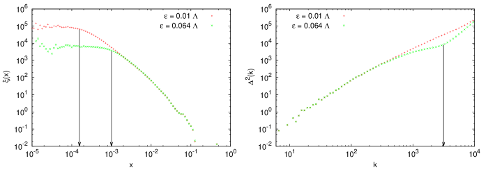
Figure 5: Comparison of results for correlation functions (top) and power spectra (bottom) in two $N=64^{3}$ simulations for the case $n=0$ and $\kappa=1$ with different force smoothing: one with $\varepsilon_{1}=0.01\Lambda$, and the other $\varepsilon_{2}=0.064\Lambda$; both of these $\varepsilon$ are indicated by the vertical lines on the plots of $\xi$, while only the scale $\pi/\varepsilon_{2}$ is marked on the power spectra plots ( $\pi/\varepsilon_{1}$ lies out of the plotted range).

3.6 Results: visual inspection

Shown in Fig.s 6 and 7 are some snapshots of the particle configurations in a few chosen simulations. In each case we show, for a given initial power spectrum, the configurations at several times $t_{s}$ for simulations with the largest and smallest simulated value of $\kappa$. As discussed above, the time variable $t_{s}$ is defined so that it corresponds to the same linear amplification of the growing mode in any model. Thus, for the same initial condition, the evolution in linear perturbation theory in the different $\kappa$ models should be identical. Further following our discussion above, we expect the non-linear structures to become more compact as $\kappa$ increases. Both expectations are evident qualitatively in the snapshots: in all cases the structures at larger scales — where perturbations are small — are indeed very similar, and in all cases we see that the effect of increasing $\kappa$ is to make the non-linear structures more compact.

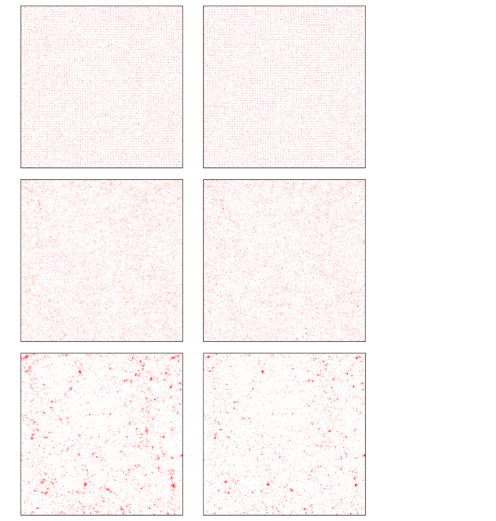
Figure 6: Snapshots (projections on plane) for initial conditions $P(k)\propto k^{-1}$, at the times $t_{s}=1.0,2.5,4.0$ for the models with $\kappa=1,2.3$ (from left to right)

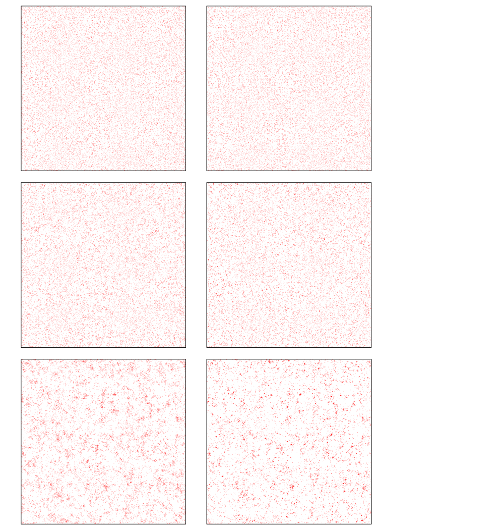
Figure 7: Snapshots (projections on plane) for initial conditions $P(k)\propto k^{2}$, at the times $t_{s}=1.0,3.0,5.0$ for the models with $\kappa=0.23,1$ (from left to right)

3.7 Results: dependence of two point correlation properties on $\kappa$

In Fig. 8 are shown our results for $\xi(x)$ and $\Delta^{2}(k)$ for all simulations when they are highly evolved. Each plot shows, for the subset of models with a fixed $n$ (but different $\kappa$), one of the two quantities at the indicated times $t_{s}$. Also shown in each of the $\Delta^{2}(k)$ plots is the prediction of linear theory, obtained by multiplying the measured $\Delta^{2}(k)$ for the initial conditions (identical for all models at given $n$) by the predicted linear theory amplification $e^{t_{s}}$. The black vertical line indicates the smoothing parameter $\varepsilon$ in the plots of $\xi(x)$, and $0.1(\pi/\varepsilon)$ in the plots of $\Delta^{2}(k)$.

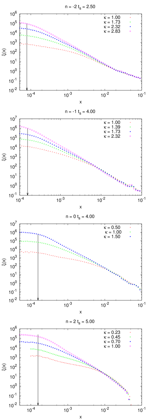
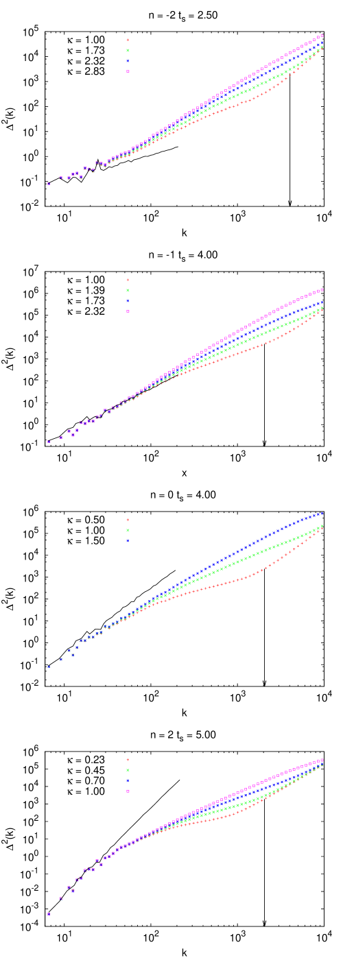
Figure 8: Plots of $\xi$ and $\Delta^{2}(k)$ at indicated times $t_{s}$ in different models. The black vertical line in each plot of $\xi(x)$ indicates the smoothing parameter $\varepsilon$. The black curve in each plot of $\Delta^{2}(k)$ shows the prediction of linear theory.

These plots confirm quantitatively what was anticipated above in the visual snapshots: the evolved configurations have indeed almost identical two point correlation properties at the larger scales at which linear theory is valid, while in the non-linear regime the effect of increasing $\kappa$ is to lead to greater relative power at smaller scales, with both $\xi(x)$ (and $\Delta^{2}(k)$) clearly increasing much more rapidly with decreasing $x$ (and increasing $k$)

These behaviours — notably a non-linear correlation function which steepens as $\kappa$ increases — are thus qualitatively in line with those predicted in the stable clustering hypothesis. We note that these results are also qualitatively in line with what one would anticipate from results of previous numerical studies of the effect of modifications of cosmology, notably by curvature and/or a cosmological constant. As discussed in Section 2, the case of an open universe or cosmological constant correspond to a $\kappa$ which becomes larger than unity at later times, and indeed it has been observed in previous studies (see e.g. Peacock & Dodds (1996); Padmanabhan et al. (1996)) that in these cases non-linear power is increased when one compares the models at times at which the linear fluctuations are identical.

Results like the ones just mentioned, and more generally the analysis of two point correlation properties, are often presented in the cosmological literature in terms of representations of $\xi$, or more often $\Delta^{2}$, as functions of variables $\xi_{L}$ or $\Delta_{L}^{2}$, representing the linearly evolved $\xi$ or $\Delta^{2}(k)$ at a length scale $x_{L}$ (or $k_{L}$) related to $x$ (or $k$) through a mapping described, e.g., in Hamilton et al. (1991); Peacock & Dodds (1996). We have performed this analysis for all our models to obtain $\Delta^{2}$ [$\Delta_{L}^{2}$], using $k_{L}=k(1+\Delta^{2}(k))^{-1/3}$. For brevity, we do not report the results here, as they do not reveal any particular simplicity additional to what we have already obtained by mapping the linear evolution working in time units defined by $t_{s}$. In particular we note that the stable clustering hypothesis, which leads to the “universal” behaviour $\Delta^{2}(k)\propto[\Delta_{L}^{2}(k)]^{3/2}$ for the usual EdS model, generalizes, given the generalized linear evolution Eq. (17), to $\Delta^{2}(k)\propto[\Delta_{L}^{2}(k)]^{3/2\alpha}$. In line with stable clustering, we indeed observe such a steepening of $\Delta^{2}(k)$ plotted as a function of $\Delta_{L}^{2}(k)$ in the strongly non-linear regime ($\Delta^{2}(k)\mathrel{\hbox to0.0pt{\lower 3.0pt\hbox{$\mathchar 536\relax$}\hss}\raise 2.0pt\hbox{$\mathchar 318\relax$}}10^{2}$) .

3.8 Results: self-similarity

To test for self-similarity in the two point correlation properties, as expressed by (22) and (23), it is convenient to plot for each simulation $\xi(x)$ and $\Delta^{2}(k)$ in the rescaled length units ($x/R_{s}$, $kR_{s}$) in which they should be identical if self-similarity holds. Shown in Fig. 9 and Fig. 10 , are these plots for a number of our simulations. Specifically for each $n$ we show results for the simulation with the smallest and largest $\kappa$ (and thus the smallest and largest $\gamma_{sc}$). The rescaling has been done taking the final time of our simulation as the reference time (i.e. for the latest time shown the length scales are the untransformed ones). Also shown in each of the $\Delta^{2}(k)$ plots is the prediction of linear theory, obtained by rescaling according to linear theory the measured value in the initial conditions. The black vertical lines indicate the scale $2\varepsilon$ in the plots of $\xi$, and the scale $0.1(\pi/\varepsilon)$ in the plots of $\Delta^{2}(k)$. Following the results and discussion of Section 3.5, these are the scales at which we anticipate that the results begin to be significantly affected by force smoothing.

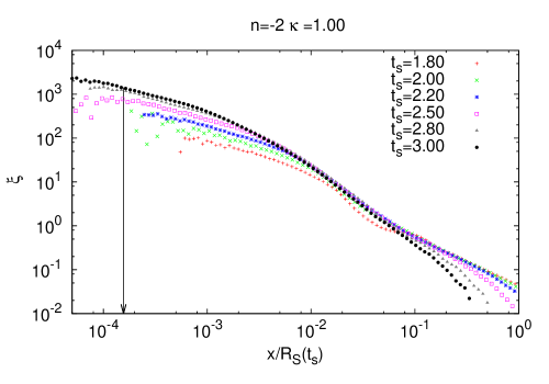
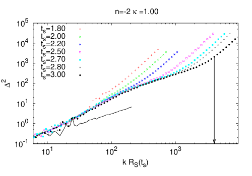
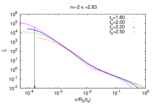
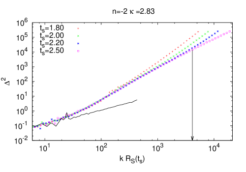
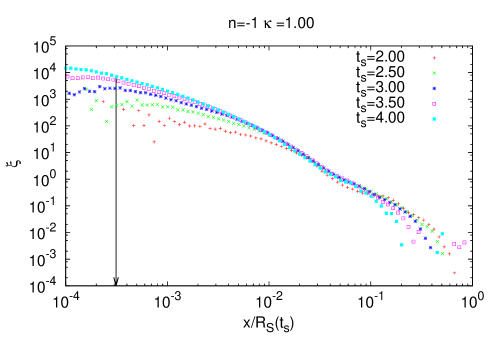
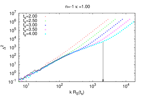
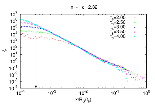
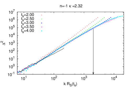
Figure 9: Each plot shows $\xi$ or $\Delta^{2}$ for a model with $n=-2$ or $n=-1$, for different times and in rescaled space variables appropriate to test for self-similar evolution. The black vertical lines indicate the scale $2\epsilon$ in the plots of $\xi$, and the scale $0.1(\pi/\varepsilon)$ in the plots of $\Delta^{2}(k)$. The black curve in each plot of $\Delta^{2}(k)$ shows the prediction of linear theory.

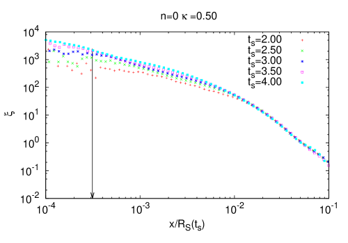
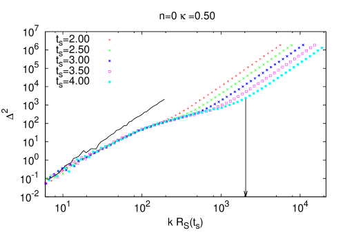
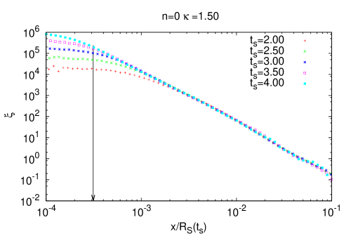
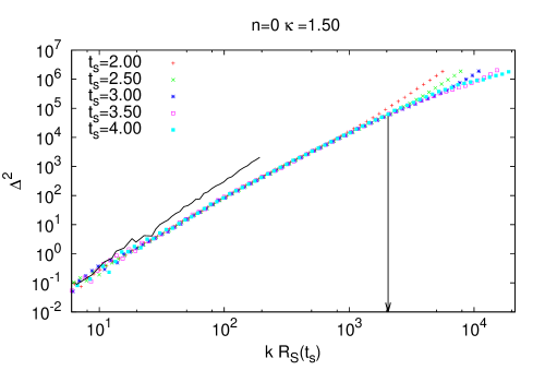
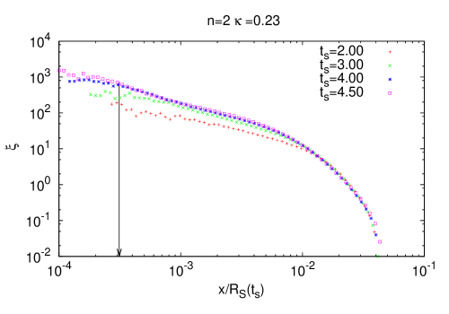
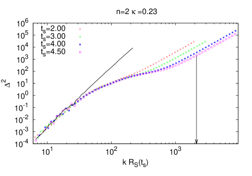
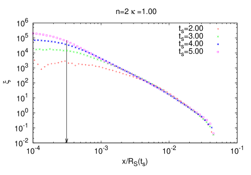
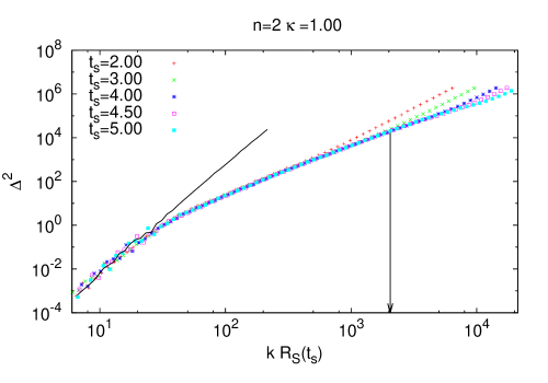
Figure 10: Each plot shows $\xi$ or $\Delta^{2}$ for a model with $n=0$ or $n=2$, for different times and in rescaled space variables appropriate to test for self-similar evolution. The black vertical lines indicate the scale $2\epsilon$ in the plots of $\xi$, and the scale $0.1(\pi/\varepsilon)$ in the plots of $\Delta^{2}(k)$. The black curve in each plot of $\Delta^{2}(k)$ shows the prediction of linear theory.

At any given time we can infer the measured $\xi(x)$ or $\Delta^{2}(k)$ to be self-similar over the range of scale over which they are well superimposed with their values at other times. In all the plots we indeed observe that, starting from the initial time, there is a region of superposition of each of $\xi(x)$ and $\Delta^{2}(k)$ with its value at the subsequent time step, and, in some cases, at all subsequent time steps. In the plots of $\xi$ the corresponding range at each time has a very clearly identifiable lower cut-off for $\xi(x)$, at a value of $\xi$ which increases monotonically in time. and, correspondingly, in the $\Delta^{2}(k)$ plots an upper cut-off at a value of $\Delta^{2}(k)$ which increases in time. These behaviours reflect the progressive establishment of self-similarity via the mechanism of hierachical structure formation well documented in the usual cold dark matter models: the transfer to smaller scales of the initial power at larger scales by non-linear evolution, which leads to self-similarity when the initial fluctuation spectrum contains only a single characteristic scale. Conversely the dependence of clustering on the details of the initial fluctuations at scales around and below $\Lambda$ is progressively wiped out (but at a rate which, as we will discuss below, clearly depends strongly on the model) Thus there is clear evidence for the asymptotic establishment of self-similar evolution in all these models. We note in particular that our results show self-similarity to apply also for the models with $n=2$ (and also for the two others not shown here). Thus, as anticipated in our discussion above in Sect. 2.3, it is clear that there is no breakdown of self-similarity above $n=1$ as has been suggested (on theoretical grounds) in some works.

The degree to which self-similarity is established varies, however, quite markedly from model to model:

• We observe, for each $n$, that comparing the two values of $\kappa$ at the same $t_{s}$, the lower cut-off to self-similarity is very significantly smaller for the case with larger $\kappa$, and the amplitude in $\xi$ (or $\Delta^{2}$) to which it extends is larger. Indeed for the cases with the smallest $\kappa$, and most notably for ($n=2,\kappa=0.23$) and ($n=-2,\kappa=1$), the region in which self-similarity can be observed is very limited, barely extending beyond $\xi\sim 10^{2}$. These results are clearly qualitatively in line with the estimates we made in Section 2.7 based on the hypothesis of (self-similar) stable clustering, with the range of non-linear self-similar correlations clearly strongly increasing as $\gamma_{sc}$ does. Analysis of the same plots for the (seven) other models, corresponding at each $n$ to the models with values of $\kappa$ intermediate between those shown here, confirm very clearly these trends, and even show rough quantitative agreement with the estimates given in Section 2.7. Notably, at given $n$, we indeed observe self-similarity develop in a logarithmic range of scale which is very consistent with a proportionality to $3/(3-\gamma_{sc})$, as predicted by Eq. (38). Comparison of these estimates for simulations at the same $\gamma_{sc}$, but different $n$, shows also good agreement, although it is complicated by the fact that the scale denoted $x_{f}$ in Section 2.7, the largest scale which has gone fully non-linear, in fact varies quite significantly as a function of $n$ in our simulations: examining, for example, the scale at which $\xi=1$ in Fig. 9 and Fig. 10 we see it is substantially larger for the cases $n=-2$ and $n=-1$ than for the two other values of $n$.

• We see also other very clear differences, in the plots of $\xi$, in the behaviour at larger scales: for the cases $n=-2$ and $n=-1$ one can clearly see that self-similarity has at each time an upper cut-off at scales well inside the box, at a value of $\xi$ which monotonically increases in time; for $n=0$ and $n=2$, on the other hand, no such upper cut-off can be detected (and this is true also in plots not shown extending to the scale of the box). In the ($n=-2,\kappa=2.83$) model self-similarity is thus visibly broken at the latest time for $\xi\mathrel{\hbox to0.0pt{\lower 3.0pt\hbox{$\mathchar 536\relax$}\hss}\raise 2.0pt\hbox{$\mathchar 316\relax$}}1$, while in the other $n=-2$ model (which extends to a larger $t_{s}$) and the two $n=-1$ models, this break extends almost to $\xi\sim 10^{2}$, with a curve at the final time in these cases slightly lower than that defined in this region by the superposition of the curves at the earlier times. This breakdown of self-similarity at larger scales is precisely in line with what one anticipate due to finite box size effects: indeed the deviations from self-similarity are much more significant for the models with $n=-2$ and $n=-1$, for which the amplitude of fluctuations at the scale of the box (cf. Table 1) are largest at the latest times, and which are expected to be most sensitive to the “missing power” at larger scales . Indeed for these cases, the higher amplitude makes it not only possible for us to detect clearly, in $\xi$, the breakdown of self-similarity at quite early times in the linear regime, but also its propagation to the point where it affects the correlations in the non-linear regime. The fact that this behaviour can be traced clearly in $\xi$, but not in $\Delta^{2}(k)$, is due to the fact that the latter is more sensitive to the contributions from the “missing modes” (i.e. below the fundamental of the periodic box), increasingly so as $n$ decreases (reflecting the infra-red divergence in the integral defining $\xi$ as $n\rightarrow-3$). Thus for $n=0$ and $n=2$ we would need to evolve the simulation much further even to be able to detect such effects in the linear regime.

• We note that the ($n=0,\kappa=0.5$) model, and to a much lesser extent the ($n=2,\kappa=0.23$) model, show a qualitatively different behaviour to the other (thirteen) models, in the strongly non-linear regime at the last time shown: there is, comparing the last two times, apparently good self-similar superposition down to a scale of order $\varepsilon$ but broken by a slight “bump” in $\xi$ at intermediate scales. We believe that these results, at least at amplitudes significantly above $\xi\sim 10^{2}$, are probably unphysical because they correlate precisely with the poorer numerical precision indicated by the data in Section 3.4, and we will take account of this in the discussion of our final results below.

It is interesting to comment on these results in relation to discussion in the previous literature (for the case $\kappa=1$) of establishing self-similarity (and evaluating the validity of stable clustering) below $n=-1$ (e.g. Efstathiou et al. (1988); Jain & Bertschinger (1996, 1998); Smith et al. (2003)). Through the study of our family of models, we see very clearly that the difficulty in establishing self-similarity (and thus testing for stable clustering) is unrelated to any intrinsic problem posed by the infra-red properties of the spectrum. Indeed we see that we have no difficulty observing self-similarity (and, as we will see, establishing that the stable clustering approximation is good) for $n=-2$ when $\kappa$ is increased, and conversely we encounter difficulty, for example, when $n=2$ when $\kappa$ is much less than unity. At the same time, we do see very clearly the effect of greater sensitivity to finite size effects for decreasing $n$, and can control for them: if self-similarity is broken only in the regime $\xi<1$, we can be very confident that these finite size effect do not modify the non-linear regime at all; and even when they lead to breaking of self-similarity to significantly larger $\xi$ — as is the case, as we have seen, in some of the simulations with $n=-2$ and $n=-1$ at the latest times — we can still always identify the part of the correlation function or power spectrum affected by it. Further direct tests for finite box size effects reported below confirm the reliability of this procedure.

3.9 Non-linear self-similar clustering: two point correlation properties

We now analyse in detail the strongly non-linear regime. More specifically we isolate the self-similar region of the measured two point correlations, and assess to what extent the two point correlation properties are in line with, or deviate from, the predictions of stable clustering. The latter, as we have discussed, predicts a region of power-law clustering $\xi(x)\sim x^{-\gamma}$ with the exponent $\gamma=\gamma_{sc}(n,\kappa)$ as given in (32). In the power spectrum such a region, if sufficiently extended in real space, will be expected to lead to a region in which $P(k)\sim k^{-3+\gamma}$, or $\Delta^{2}(k)\sim k^{\gamma}$. We privilege the real space analysis, using the two point correlation function $\xi(r)$, for the reasons illustrated by our analysis in Section 3.5: we can be confident the effect of the force smoothing is clearly localized in direct space, while this may not be the case in reciprocal space. However we perform also the reciprocal space analysis, to see the consistency of our results, and also for the purposes of comparison with other studies.

In each simulation we perform our analysis in the following steps:

• We extract the correlation function $\xi_{f}(x)$ at the final time $t_{s}^{f}$ (as in Table 1), and the correlation function $\xi_{f-1}(x)$ at a slightly earlier time, $t_{s}^{f}-\Delta t_{s}$. For the $n=-2$ simulations we have taken $\Delta t_{s}=0.3$, and $\Delta t_{s}=0.5$ for the others.

• We perform the self-similar scaling on $\xi_{f-1}(x)$ to the time $t_{s}^{f}$, and comparing it with $\xi_{f}(x)$, we determine a scale $x_{ss}$ below which the rescaled $\xi_{f-1}(x)$ deviates by more than ten percent from $\xi_{f}(x)$. This defines what we take to be the lower cut-off to self-similarity.

• We examine the correlation function $\xi_{f}(x)$ above the scale $x_{ss}$ and perform a power law fit in the region in which such a fit appears by eye to be reasonable. In all simulations this is the case if we take an upper cut-off for the fit at $\xi\sim 10^{2}$, which is very consistent with the assumption that this upper cut-off marks the transition to a quasi-linear regime. In the cases $n=-2$ and $n=-1$ this upper cut-off scale to the power law fit is always smaller than the upper cut-off to self-similarity due to finite size effects.

• We determine a second scale $x_{ss}^{\prime}<x_{ss}$ by extrapolating $x_{ss}$ assuming stable clustering applies between $t_{s}^{f}-\Delta t_{s}$ and $t_{s}^{f}$ at the physical scale associated with it at $t_{s}^{f}-\Delta t_{s}$. We perform a new power law fit, using max [$x_{ss}^{\prime}$, $2\varepsilon$] as the lower cut-off and the same upper cut-off as for the first fit.

This procedure is illustrated in Fig. 11 for one case ($n=0,\kappa=1$). We note that in this procedure the interval $\Delta t_{s}$ needs evidently to be chosen large enough to allow the identification of a lower cut-off scale to self-similarity above $2\varepsilon$. To optimize the extraction of information about self-similarity in our data, on the other hand, it should be chosen as small as possible. The values we chosen for $\Delta t_{s}$ given are in practice sufficiently close to such an optimum: in the (lower $\gamma_{sc}$) cases where $x_{ss}^{\prime}$ is larger than $2\varepsilon$, we have checked that our measured values (and the error bars we estimate) below do not change significantly if we use smaller $\Delta t_{s}$ (we have data at times intervals in $t_{s}$ of $0.1$).

For the $k$ space analysis, we have identified by eye in each self-similarity plot a value of $k$ up to which the $\Delta^{2}(k)$ at the final time overlaps well with that at $t_{s}^{f}-\Delta{t_{s}}$ (using the same values of $\Delta{t_{s}}$). A power law is then fitted between this point over the region where such a fit appears reasonable, which again corresponds in all cases to a cut-off at an amplitude consistent with the transition to a strongly non-linear virialized regime. We have also limited ourselves to the region $k<0.1(\pi/\varepsilon)$.

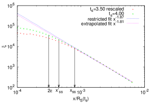
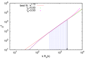
Figure 11: Plots showing our fitting procedure for the non-linear self-similar correlations for one model ($n=0,\kappa=1$): for $\xi$ we perform a “restricted fit” and an “extended fit” using two lower cut-offs (indicated by arrows) determined as described in the text; for $\Delta^{2}$ we perform a fit over the range of self-similarity as determined by visual inspection.

n	$\kappa$	$\gamma_{sc}$	$\gamma_{\rm restricted}$	range	$\gamma_{\rm extrapolated}$	range	$\gamma_{\Delta^{2}}$	$\overline{\gamma}$	$\Delta\gamma$
-2	1.00	1.00	1.13	0.25	1.04	0.47	1.05	1.07	0.05
-2	1.73	1.50	1.55	0.75	1.51	1.10	1.52	1.53	0.02
-2	2.32	1.80	1.79	1.00	1.78	1.35	1.78	1.78	0.01
-2	2.83	2.00	2.11	0.65	2.07	1.10	2.08	2.09	0.02
-1	1.00	1.50	1.61	0.35	1.51	0.65	1.40	1.51	0.1
-1	1.39	1.80	1.89	0.80	1.83	1.20	1.78	1.83	0.06
-1	1.73	2.00	2.13	0.85	2.10	1.10	2.00	2.08	0.07
-1	2.32	2.25	2.42	0.95	2.42	1.00	2.27	2.37	0.08
0	0.50	1.21	1.37	0.25	1.29	0.40	1.06	1.24	0.16
0	1.00	1.80	1.87	0.90	1.81	1.20	1.72	1.80	0.08
0	1.50	2.14	2.27	1.25	2.27	1.30	2.12	2.22	0.08
2	0.23	1.00	0.94	0.76	0.95	0.80	1.10	1.00	0.08
2	0.45	1.50	1.58	0.16	1.46	0.32	1.49	1.51	0.06
2	0.70	1.87	1.89	0.80	1.86	1.15	1.80	1.85	0.04
2	1.00	2.14	2.26	0.80	2.31	1.10	2.18	2.25	0.07

Table 2: Theoretical prediction $\gamma_{sc}$ for exponent charactering non-linear self-similar two point correlations in each model, and the three values measured from simulations as described in the text. For the two fits to the correlation function the spatial range of the fit is given in the form $log\frac{x_{max}}{x_{min}}$. The last two columns give the average of these three measures, and an error bar given by half the maximum difference between the three measures.

The results of this analysis are given in Table 2. For each simulation it gives the exponent obtained from the two fits to the correlation function (“restricted” and “extrapolated”), as well as the range in which these fits are performed following the procedure described. Also given is the best fit exponent obtained in the $k$ space analysis. For all of these exponents a standard fitting procedure gives a statistical error bar ranging between $\pm 0.02$ to $\pm 0.005$. Examining the results we see that overall the measured exponents show in all cases, within roughly $\pm 0.1$, agreement with the prediction of stable clustering. Some slightly larger deviations are seen in a few cases (up to $\pm 0.2$), but they are associated with a dispersion of the same order in the exponents estimated in reciprocal space. In other words, taking the dispersion of the exponents obtained with the different fitting methods as indicative of a (dominating) systematic error bar, all our results are quite consistent with the stable clustering hypothesis, and exclude deviations of at most about $\pm 0.15$. To quantify the comparison between the predicted and measured exponents succinctly, the last two columns in Table 2. give the results of the measurements in the form of an estimated exponent and error bar, with the former given by the average of the three measured exponents and the latter by half the maximum dispersion of the three mesures of the exponent. In several cases, agreement with the stable clustering prediction within $\pm 0.05$, or even considerably less. The largest error bar — reflecting a large dispersion between the real and Fourier space estimates — is for the case $(n=0,\kappa=0.5)$, for which we have noted the late time behaviour is probably affected by poor numerical precision. The only case showing possibly significant discrepancy with the theoretical exponent are the models $\gamma_{sc}\geq 2$, which all have estimated values marginally above the theoretically predicted one. On the basis of a more extended analysis of the energy evolution parameters and other simulations, which we will report in detail elsewhere, we believe that there is indeed such a systematic effect but that it is numerical in origin, linked to the difficulty of simulating accurately into the regime where the smallest structures “shrink” below the force smoothing, which is the case in these models.

Shown also in Fig. 12 and 13 are the $\xi(x)$ at the latest time, for all simulations. In each case are plotted also a line showing our best “extended fit” as well as a best fit (by eye) to the exact stable clustering prediction, and the range of scales in which the fit is performed. The results of the quantitative analysis using the estimated error bars are clearly very coherent with what be observed by visual inspection of these curves: excellent agreement with stable clustering within error bars which are typically larger for the smaller $\gamma_{sc}$ simulations, for which the physical (i.e. self-similar) non-linear correlations may be measured only in a very narrow range of scale. We note that the ($n=0,\kappa=0.5$) simulation is fitted in a region excluding most of the range in which we observed unusual behaviour in our discussion in Section 3.8, while the model ($n=2,\kappa=0.23$) is fitted in a surprisingly large range, as the small “bump” feature noted also in this model is not excluded from the self-similar fit by our criterion of a ten percent discrepancy. We believe that the real systematic error in this particular case — due probably to poor numerical precision indicated by $A_{1}$ — is therefore larger than that estimated in Table 2.

We underline that, as can be seen in Figs. 12 and 13, the criterion of self-similarity is in practice crucially important in allowing us to identify the appropriate lower cut-off to the range of scale in which the simulated correlation function can be taken to represent the physical (self-similar) correlation function. Indeed, while for the larger $\gamma_{sc}$ models the determined lower cut-off extends down to $2\varepsilon$, i.e., down to the scale which we would assume automatically be a lower cut-off on resolution of clustering due to force smoothing, this in not the case for the models at smaller $\gamma_{sc}$. In most of these models there is a very significant range of scale above $2\varepsilon$ — up to as much as a decade in a few cases — in which the clustering signal measured in the simulation is not self-similar, and therefore (we assume) not physical. This means that in this range of scale the measured correlations are unphysical transients from the initial conditions, in which notably the characteristic scale $\Lambda$ in the initial conditions is imprinted. Conversely, for these simulations, we can conclude that no extra physical information has been gained by using the small force smoothing we have employed, while for the larger $\gamma_{sc}$ the strong constraints on the non-linear correlations we have obtained are a result of this choice.

In summary, our conclusion is thus that, in the regime where we can measure with confidence the non-linear and self-similar correlation function of these models using our simulations, it can be fit well in the models we have simulated by the stable clustering hypothesis.

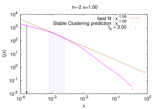
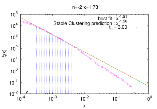
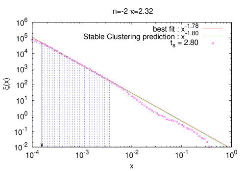
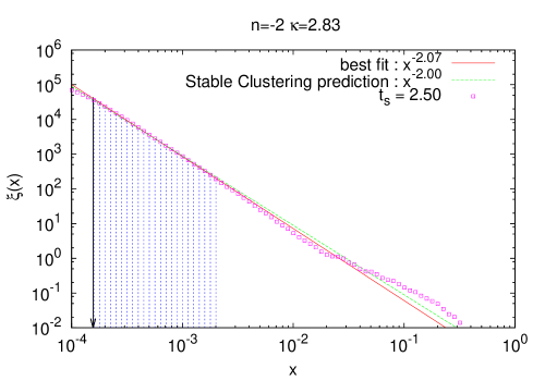
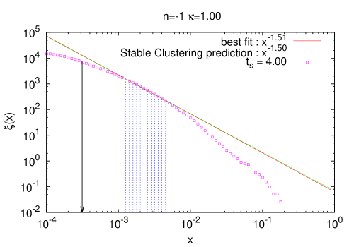
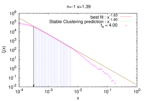
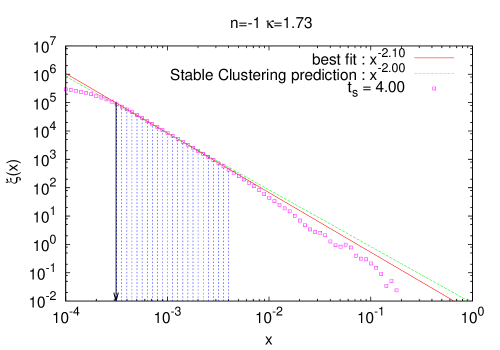
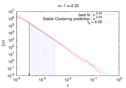
Figure 12: Plots for $\xi$ at the latest simulation time in each given model, along with lines corresponding to our best “extrapolated fit” and the prediction of stable clustering, in the range indicated by the vertical blue lines. The black vertical line gives the scale $2\varepsilon$.

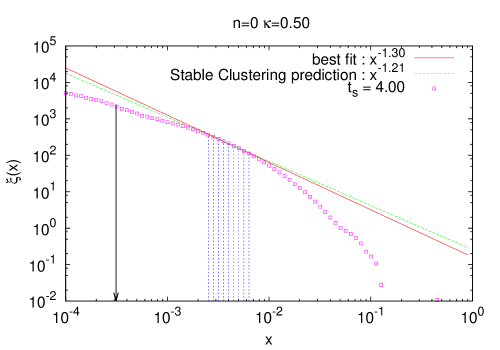
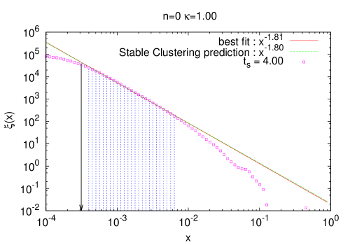
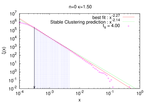
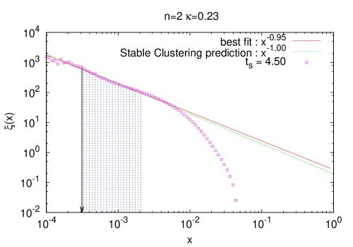
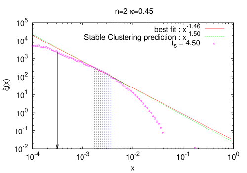
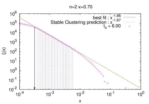
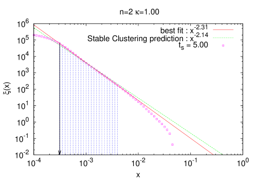
Figure 13: Plots for $\xi$ at the latest simulation time in each indicated model, along with lines indicating our best “extrapolated fit” and the prediction of stable clustering.

3.10 Direct tests for finite box size effects

As we have discussed above, the restriction of our measurements of the correlation function and power spectrum to the scales in which these quantities are self-similar should ensure that our results are unaffected by effects arising from the finite size of our simulation box. Indeed, for our models with $n=-1$ and $n=-2$ in which we expect such effects to be most important, our tests for self-similarity have identified clearly the presence of such effects at larger scales. It is interesting to test also more directly for finite size effects by using simulations which are identical other than for the simulation box size, and in particular to verify that the correlation function and power spectrum are indeed unaffected by the box size in the range of scale indicated by the test of self-similarity.

To perform such a test we have resimulated the model with $n=-1$ and $\kappa=1$ (i.e. EdS) with $N=256^{3}$ particles (starting from the same amplitude of initial fluctuations as given in Table 1). For one simulation we have used the same smoothing ($\varepsilon=0.01$) as in our fiducial simulations, and for the other a larger smoothing ($\varepsilon=0.03$). Shown in Fig. 14 are the measured $\xi(r)$ and $\Delta^{2}(k)$ in these two simulations at the time $t_{s}=4$ alongside those for the simulation with $N=64^{3}$ used in our analysis above, at the same time.The comparison between the two simulations with $\varepsilon=0.01$ shows that there are indeed significant finite size effects at scales which are large but well inside the box size at this time. Indeed, in excellent agreement with what we have inferred from our analysis using self-similarity of the smaller simulation, these effects extend at this time (the latest time used for our analysis above) down to scales in which $\xi\sim 10^{1}$ – $10^{2}$. It is interesting to note also that the peculiar “bump” feature at $\xi\sim 1$ in the $64^{3}$ simulation clearly disappears in the larger box simulation, and is indeed unphysical as one would anticipate (in a scale-free model).

The comparison of the two simulations with $N=256^{3}$ with different smoothing is shown as it confirms further the conclusions of the analysis in Sect. 3.5: we see that the correlation functions for the two simulations agree very well down to close to the larger $\varepsilon$, while in $\Delta^{2}(k)$ the effect of the smoothing in decreasing the power is clearly visible already at $k\approx 0.1(\pi/\varepsilon)$. The exponent $\gamma$ obtained fitting either simulation in the self-similar region gives a value very consistent with that obtained from the $64^{3}$ simulations.

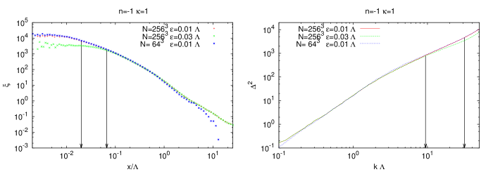
Figure 14: Comparison of $\xi(r)$ (left) and $\Delta^{2}(k)$ (right) in three simulations of the model $n=-1$ and $\kappa=1$, at the time $t_{s}=4$, and starting from an amplitude of initial fluctuations given in Table 1. One pair of simulations differ only in particle number (i.e. box size), while the pair at $N=256^{2}$ differ only in force smoothing. The $x$-axis in both plots has been rescaled to the initial grid spacing $\Lambda$, and the black vertical lines indicate the values of $\varepsilon$ on the plots of $\xi$, and those of $(0.1)\pi/\varepsilon$ on the plots of $\Delta^{2}(k)$.

4 Discussion and conclusion

In this final section we first give a brief summary of our most important results and conclusions. We then compare our results to some previous studies in the literature (of the $\kappa=1$ case). We conclude with a brief discussion of the possible implications of our study, in particular in relation to the issue of “universality” of gravitational clustering in cosmological models, and then trace finally some directions for future research.

4.1 Summary of main results

• We have pointed out the interest in studying structure formation in a family of EdS models, noting that, like the canonical case, they are expected to display, for power law initial conditions, the property of self-similarity. The latter provides a powerful tool to distinguish the physically relevant results of a numerical simulation: where the observed clustering is not self-similar, it is necessarily dependent on the length and time scales which are introduced by the finite simulation. This family of models allows us to investigate in such a context not just, as in the usual EdS model, the dependence on initial conditions of clustering, but also the dependence on cosmology.

• We have derived in these models both the theoretical predictions for the self-similar behaviour, and those for the exponents $\gamma_{sc}(n,\kappa)$ characterising the non-linear regime in the additional hypothesis of stable clustering.

• We have explained that the (theoretical) exponent $\gamma_{sc}(n,\kappa)$ has a very simple physical meaning: it controls the relative size of virialized structures compared to their initial relative comoving size. Larger $\gamma_{sc}(n,\kappa)$ corresponds thus to a greater “shrinking” of substructures contained in a given structure. It follows that we expect $\gamma_{sc}(n,\kappa)$ to be a good control parameter for the validity of stable clustering, and also for the range in which it can be observed in a finite simulation (if it is a good approximation).

• We have reported the results of an extensive suite of $N$ body simulations, performed using an appropriate modification of the GADGET2 code which we have implemented and tested. To control the code’s relative accuracy in different simulations we have defined a suitable generalized variant of the usual test based on the Layzer-Irvine equation.

• We have analysed in detail the two point correlation properties in real and reciprocal space of the evolved distributions for models covering a broad range in the $(n,\kappa)$ parameter space. Our chosen range in $n$ extends to the region $n>1$ which has not been studied previously even in the standard ($\kappa=1$) case. Our results show that all our models display a clear tendency to establish self-similar evolution over a range of comoving scale which grows monotonically in time. Further, we find that in all cases the self-similar region of the fully non-linear part of the correlation function (and power spectrum) are well fit by a simple power law from with an exponent in good agreement with the prediction of stable clustering. As anticipated theoretically, the robustness and range of validity of these numerical results turns out itself to be a function of $\gamma_{sc}$: as it decreases below $\gamma_{sc}\approx 1.5$ the range of strongly non-linear self-similar clustering diminishes considerably, so much so that at $\gamma_{sc}\approx 1$ the prediction of stable clustering can only be marginally tested. Given these limitations we are not able to detect any deviation from the stable clustering prediction in this class of models, and conclude that significantly larger simulations would be needed to do so.

4.2 Comparison with other studies

4.2.1 Three dimensions

Previous studies have considered the usual EdS model for different values of $n$ in the range $-3<n\leq 1$, focussing both on the validity of self-similarity and stable clustering.

Concerning self-similarity our results are in agreement with all previous studies for this range, but help to clarify two questions. Firstly they show that for the usual EdS model self-similarity indeed extends to $n>1$. We have studied only the case $n=2$, but we can be extremely confident, given the observed trend with $n$, numerical results in the one dimensional case (Joyce & Sicard (2011); Benhaiem et al. (2013)), and the theoretical considerations concerning $\gamma_{sc}$, that this result extends up to $n=4$. Secondly, our results throw light on the difficulty, documented and discussed in the previous literature, of observing self-similarity in numerical simulations in the range $-3<n<-1$, which even led to the suggestion that it might not apply for this case because of infra-red convergence of possibly relevant physical quantities (Jain & Bertschinger (1996, 1998)). Our study shows very clearly that the difficulty in observing self-similarity is not due to any intrinsic problem related to infrared properties of these spectra. Indeed we have no difficulty observing self-similarity over an extensive range even for a model with $n=-2$ when the cosmology is modified. The difficulty of observing self-similarity is due essentially just to the very limited range in which strongly non-linear clustering can develop in simulations of limited size as $n$ decreases: quite simply the range of scale factor which can be simulated is so small that the increase in the density contrast in stable clustering is very small. The relative degree of this difficulty for different models is, as we have explained, well characterized by the theoretical stable clustering exponent of the model.

Concerning the validity of the stable clustering hypothesis as tested by comparison with its predictions for the two point correlation properties, our conclusions are in disagreement with the most recent major study of the issue, that of Smith et al. (2003). This article considers the cases $n=0,-1,-1.5,-2$ in the usual EdS model, and reports results of an analysis of two point properties showing, in all cases, significant deviations from the predictions of stable clustering, characterized by the measurement of exponents significantly smaller in all cases than the ones predicted by stable clustering: for $n=0$, $\gamma=1.49\pm 0.05$ (compared to $\gamma_{sc}=1.8$); for $n=-1$, $\gamma=1.26\pm 0.1$ (compared to $\gamma_{sc}=1.5$); for $n=-2$, $\gamma=0.77\pm 0.15$ (compared to $\gamma_{sc}=1$). Comparing these results and our results in Table 2, it is not evident, given the roughness of the error bar estimates, whether there is really a strong discrepancy with our results as described above for the case $n=-2$ and $n=-1$. The results for the case $n=0$ is, however, are most definitely strongly at odds. Indeed we found in this case that all three fitting procedures give an exponent within $0.1$ of the predicted value, and evidently Smith et al. (2003) very strongly exclude a fit to an exponent in this range. On the other hand, the slightly earlier study of the case $n=-2$ of Jain & Bertschinger (1998) concludes, like us, that the two point correlation properties are in this case in line with the prediction of stable clustering, while Smith et al. (2003) clearly state that their result is discrepant also with this result (and propose an explanation for this discrepancy which we will discuss further below).

Let us compare more closely the different studies. The analysis and conclusions of both Smith et al. (2003) and Jain & Bertschinger (1998) are obtained from simulations with $N=256^{3}$ particles, while we have used $N=256^{3}$ for only one model and $N=128^{3}$ or $N=64^{3}$ otherwise. On the other hand, we have used a softening $\varepsilon$ which, in units of the initial interparticle spacing $\Lambda$, is approximately the same as that of Jain & Bertschinger (1998) but smaller by a factor of six than that of Smith et al. (2003). The overall spatial range potentially resolved, strictly bounded below by $\varepsilon$ and above by the box size, is thus largest for the $n=-2$ ($\kappa=1$) simulation of Jain & Bertschinger (1998) and our ($n=-1$, $\kappa=1$) simulation, and smallest for Smith et al. (2003), with our simulations simulations intermediate between the two. In practice, however, we must compare the different results taking account of the range of scale in which non-linear structure is actually simulated in each case, and assess whether systematic effects can explain the differences between them. Laying aside the possibility of any significant discrepancies in the numerical integration, such systematic effects are either (i) finite size effects associated with the periodic box, or (ii) force resolution effects associated with the force smoothing.

In their discussion of Jain & Bertschinger (1998), Smith et al. (2003) argue that the discrepancies of their results (for the case $n=-2$) arise from finite size effects: on the basis of a simple theoretical estimate of the effect of “missing power” (associated with modes below the fundamental) in the mass variance, they argue that to avoid significant finite size effects a simulation should be evolved at most until $\Delta_{L}^{2}(k_{b})\approx 0.04(n+3)$. They note that Jain & Bertschinger (1998) evolves, and measures the compatibility of the non-linear power spectrum with stable clustering, up to a time when $\Delta_{L}^{2}(k_{b})\approx 0.4$, an order of magnitude larger than this bound admits, while their own simulations for $n=-2$ are stopped just when this bound is absorbed. As can be seen from Table 1, our final value for $\Delta_{L}^{2}(k_{b})$ is about half that of Jain & Bertschinger (1998) for $n=-2$ and five times larger than the bound proposed by Smith et al. (2003), for $n=-1$ our final value is about twice that of the bound, while for $n=0$ ($n=2$) our final value is significantly (far) below the bound.

In our analysis we have seen that finite size effects may be observed directly in simulations through the breaking of self-similarity at large scales in the correlation function $\xi$, and we have confirmed the reliability of this method for identifying these effects through direct comparison with a large simulation in Section 3.10. We have noted that the behaviours we observe of these effects are qualitatively in line with what would be anticipated from the criterion of Smith et al. (2003) — finite size effects are clearly detected for $n=-2$, and also for $n=-1$, and they not detectable for the other cases. However, even though at the final time in the $n=-2$ and $n=-1$ simulation, the breaking of self-similarity has spread beyond $\xi\approx 1$ well into the non-linear region, these effects have not propagated into the region of very strong clustering, which remains self-similar. It is in this range which we measure the correlation function exponent. Further we have checked that, when we perform our analysis using as final time one at which the bound of Smith et al. (2003) is satisfied, we still obtain an exponent — albeit over an even more limited range — consistent with our quoted result (and with stable clustering). In short our analysis leads us to conclude that, although finite size effects are clearly present in the simulations with $n=-2$ and $n=-1$ at the final times, they cannot explain the discrepancy between our measured results and those of Smith et al. (2003).

As we have noted the clearest discrepancy between our results and those of Smith et al. (2003) is for the case $n=0$, in which clearly finite size effects have, in any case, no role. If the numerical results of both studies are correct, the only possible systematic effect which can explain the difference in the measured exponents is one arising from the force smoothing. In principle we have controlled carefully for such effects by always identifying a lower cut-off scale at which self-similarity applies, and down to which we measured exponents. Further we have always checked that, in both real and Fourier space, that this scale is above that at which we expect smoothing to cause deviations. As discussed in Section 3.5, and illustrated in Fig. 5, this scale in real space can be taken to be about $2\varepsilon$, while in reciprocal space it may be very much smaller than one might naively expect. Indeed we have seen through direct comparison of simulations differing only in force smoothing — for the $n=0$ EdS model at the final in Fig. 5, and the $n=-1$ EdS model in Fig. 14 — that the the power spectrum is significantly suppressed below its true value above $k\sim 0.1\pi/\varepsilon$. From what can be inferred from the discussion given in Smith et al. (2003), it appears that the quoted results for the exponents have been derived from a Fourier space analysis only, and considering as only relevant lower cut-off scale one of order $\pi/\varepsilon$ . It is very evident from Fig. 5 (and, likewise from Fig. 14, for the case $n=-1$) that extrapolating a fit to $\Delta^{2}(k)$ much beyond about one tenth of $\pi/\varepsilon$ will lead to a lower fitted exponent, as reported by Smith et al. (2003). Thus we believe that the exponents reported by Smith et al. (2003) significantly below the stable clustering prediction are a result of including in the fitted region at least some points at which the power is suppressed significantly by smoothing. Given our conclusions about finite size effects in the cases $n=-1$ and $n=-2$, it appears probable to us that the same effect explains the measurement by Smith et al. (2003) of exponents lower than those predicted by the stable clustering hypothesis in these cases, and even lower than our average measured exponents in these cases. As we have discussed self-similarity itself should provide a “protection” against such effects, and in particular a careful identification of the lower cut-off to self-similarity and how it evolves in time. Such an analysis has not apparently been performed in Smith et al. (2003), and in particular not in real space in which the effects of smoothing can be controlled for more easily. The importance of the determination of this lower cut-off, even in real space, is illustrated well by the plots of $\xi$ for the EdS models ($\kappa=1$) in Fig. 12: there is a significant part of the measured correlation function well above $\varepsilon$, with an effective exponent well below that of the stable clustering region, which is not self-similar and which must be excluded from our fit. If this region beyond the “bending” in the correlation function is self-similar, we would need to see the scale at which this bending take place remain fixed in the self-similarity rescaling plots. This is definitely something we have not observed in our simulations of these models: in our self-similarity plots the bending scale is clearly always moving to smaller scales, and there is therefore always, as we have emphasized at the end of Section 3.9, an identifiable region where the clustering measured at smaller scales is not self-similar, and therefore cannot be taken to represent the physical clustering of the self-similar model. We note finally that Smith et al. (2003) report their derivation of exponents using the commonly used representation of $\Delta^{2}(k)$ as a function of the variable $\Delta_{L}^{2}(k_{L})$ (following the ansatz of Peacock & Dodds (1996)). We have checked our results also in this representation and find results in agreement with those of our direct analysis of $\xi(x)$ and $\Delta^{2}(k)$, i.e., we find, restricting to the region in which self-similarity is observed (to which we always detect a clear lower cut-off) an exponent in the strongly non-linear region in agreement with stable clustering.

4.2.2 One dimension

It is interesting to compare our results with those of Benhaiem et al. (2013), which performed the exactly analogous study of the one dimensional version of this class of models. Compared to the three dimensional case, this model has the interest of admitting “exact” numerical integration (i.e. limited only by numerical roundoff) and much greater spatial resolution than in three dimensions at very modest numerical cost. Thus, for example, in certain cases a strongly non-linear correlation function extending over as much as four orders in magnitude is obtained. While the same qualitative difficulties are observed as in three dimensions — the range of non-linear scales accessible in a simulation of given size shrinks rapidly as $\gamma_{sc}$ (in its one dimensional version) decreases — this greater spatial resolution makes a crucial difference in the study: we are able to clearly identify in one dimension a value of $\gamma_{sc}$, roughly at $\gamma_{sc}\approx 0.15$, above which the stable clustering approximation works very well, and below which the correlation function appears to become independent of both $n$ and $\kappa$, i.e., there is apparently a truly universal region at sufficiently small values of $\gamma_{sc}$. Further we note that the study of Baertschiger et al. (2007a, b, 2008) of the static case ($\kappa=0$) in three dimensions, for the case $n=2$ and $n=0$, finds evidence that in this limit the non-linear correlation function, albeit in a limited range of amplitude where it can be measured, is independent of initial conditions. This latter result, and those in one dimension, thus suggest that in three dimensions there is probably likewise a region in the $(n,\kappa)$ space where the strongly non-linear two point correlation function is indeed truly universal, independent of both initial conditions and cosmology. We have not been able to determine whether this region exists in this study, but significantly larger simulations might do so.

4.3 Perspectives

We finally mention some questions and directions for future work with this class of models.

• Analysis with other tools, notably halos: In this paper we have focussed solely on the characterization of clustering with two point correlation statistics. Non-linear clustering — and in particular its compatibility with the stable clustering approximation — can evidently be probed with many other statistical tools: higher order correlation functions, box counting statistics and associated fractal dimensions, etc., and scale free models are particularly interesting in that a careful separation of the self-similar part of the signal can be used to select the numerically resolved region. In the cosmological context a widely used, albeit less precisely defined statistical tool, is an analysis in terms of “halos” through appropriately defined numerical algorithms which select non-linear, and approximately virialized, clumps and characterize the density field in terms of their density profiles. Apparent “universality”, of non-linear clustering,i.e., independence of both cosmology and initial conditions — in particular in terms of mass and phase space density profiles of halos — have been extensively described in numerical simulations (Navarro et al. (1996, 1997); Taylor & Navarro (2001); Moore et al. (1999)) and much discussed in the literature. The degree of, and indeed origin of, such a putative universality remains an open and important question. The set of models we have studied here provide a very well defined framework in which to address these questions, within the very constrained setting of self-similar models. Indeed the usual EdS model with power law initial conditions has been considered as an important reference model for the study of halo properties’ dependence on initial conditions Navarro et al. (1997); Knollmann et al. (2008). In principle a universality of halos profiles requires a breakdown of stable clustering, as simple halo models are compatible with stable clustering predictions for correlation functions only if their profiles depend also on initial conditions (see e.g. Ma & Fry (2000); Yano & Gouda (2000)).

• Larger simulations: It is evident that significantly larger simulations of this class of models than those which we have reported here — say with characteristics like those of the current largest cosmological simulations (e.g. Springel et al. (2005); Alimi et al. (2012)) may be able to resolve clearly the most interesting, and indeed relevant, questions. We have only been able to establish that the fully non-linear, and self-similar, part of the correlation function which we can access with our simulations can be described well in all cases by the predictions of stable clustering. Amongst the goals of such a larger study would be the following. Firstly, for the cases ($\gamma_{sc}\mathrel{\hbox to0.0pt{\lower 3.0pt\hbox{$\mathchar 536\relax$}\hss}\raise 2.0pt\hbox{$\mathchar 318\relax$}}1$) where we have observed a region of power law clustering in line with the stable clustering prediction, to try locate a lower cut-off scale to its validity. Indeed as we have discussed, at any given $(n,\kappa)$, we would expect there must be such a cut-off as the assumption that a structure is stable must break down at some finite time (due to merging). Such a detection would require the identification of a scale, with a self-similar scaling, marking a break from the power law behaviour of the correlation, and which can be given as some fraction of the non-linearity scale. Secondly, in the region of smaller $\gamma_{sc}\mathrel{\hbox to0.0pt{\lower 3.0pt\hbox{$\mathchar 536\relax$}\hss}\raise 2.0pt\hbox{$\mathchar 316\relax$}}1$ where we have been unable to place any constraint, to measure the correlation function to higher amplitudes and assess whether it can be described in any range by stable clustering; in principle we expect to see at some point a complete breakdown of this approximation, and perhaps a tendency to a result which is completely universal, i.e., independent of $n$ and $\kappa$. Thirdly, to determine the properties of halos in these models and understand in detail their relation to two-point (and possibly higher order) correlation properties, with particular attention to the adequacy of the approximation of the distribution by smooth halos.

• Application to “realistic” cosmologies: The ultimate goal of this research is of course to contribute to a better understanding of the non-linear regime of models with initial conditions and cosmological evolutions like those in “realistic” models. In this respect we note that in principle a huge class of such models (e.g. any homogeneous dark energy model) should be characterized by a trajectory in the space $(n,\kappa)$, through the values of these quantities defined at each time by the instantaneous value of $\kappa$ defined by the expansion rate, and the logarithmic slope of the power spectrum at the scale of non-linearity. Indeed numerous existing results in the literature on different (non self-similar) models can probably be unified and understood in a simple framework in this way: for example, the observation that in both open universe models and those with a cosmological constant, non-linear clustering is amplified compared to that in the EdS model (see e.g. Peacock & Dodds (1996)), and that stable clustering becomes a better approximation in an open universe models (Padmanabhan et al. (1996)). Further, if a much fuller description of the self-similar non-linear clustering in the $(n,\kappa)$ space can be obtained, and leads to the identification of a truly “universal region” in this space, this trajectory would probably allow conclusions to be drawn about any model with respect to universality, and also the relevance of stable clustering. In this respect we note that the region of $\gamma_{sc}\mathrel{\hbox to0.0pt{\lower 3.0pt\hbox{$\mathchar 536\relax$}\hss}\raise 2.0pt\hbox{$\mathchar 316\relax$}}1$, where we have been unable to place any constraint on the non-linear regime, is a part of the $(n,\kappa)$ space which is extremely relevant to viable cosmological models: in $\Lambda$CDM (or similar models with a dynamical dark energy component) the slope of the power spectrum of initial fluctuations relevant to structure formation varies in the range from $n=-1$ to $n=-3$, and the effective value of $\kappa$ is in the range between $1$ and $\approx 2$ (see Fig. 1).

  We have not analysed the quasi-linear regime carefully, but analysis in these models, and in particular as a function of $\kappa$ at fixed $n$, may provide stringent tests of various phenomenological and/or theoretical proposal which have been made to understand it (Padmanabhan (1996)) and phenomenological fitting procedures (Peacock & Dodds (1996)). Closer to the linear regime, these models may also provide a powerful tool to test perturbative approaches beyond linear order, e.g., using the “renormalized perturbation theory” of Crocce & Scoccimarro (2006). Finally, using a description of a models as a trajectory in the $(n,\kappa)$ space, it would be interesting to try to construct, using the kind of approach developed in in Hamilton et al. (1991); Peacock & Dodds (1996), alternative semi-analytical models for non-linear clustering.

• Testing for discreteness effects: As we have underlined, the self-similarity of evolution in such models is potentially a powerful tool to study and control to what extent $N$ body simulations can be confidently taken to really reproduce, as required, the clustering in the continuum (Vlasov-Poisson) limit: indeed any deviation from self-similarity implies a dependence on scales introduced by the $N$ body method — amongst which, notably, the particle discreteness scale $\Lambda$ and force smoothing $\varepsilon$. The importance of understanding better the importance of such effects, and how they may depend notably on the model simulated, is evident from the difficulties observed in reproducing self-similarity in the limit of smaller $\gamma_{sc}$, which is the regime extremely relevant to all current realistic models. Further the confidence we have that stable clustering should apply in some of them, could potentially also be used as a strong test. We note that a few cases of the usual EdS model have been exploited in this way in studies focussing on the effects of discreteness such as Melott et al. (1997); Splinter et al. (1998); Kuhlman et al. (1996), and also on finite size effects Orban (2013b, a). In the spirit of these studies, it would be very interesting also to use this class of models to test more directly whether it is indeed reasonable to simulate in the regime $\varepsilon\ll\Lambda$, which has been a specific subject of debate in the literature (see e.g. Joyce et al. (2008) and references therein). Despite the considerable numerical challenge, it may be feasible to probe a range of non-linear clustering even with $\varepsilon>\Lambda$, for larger values of $\gamma_{sc}$ and see if they match the self-similar stable clustering behaviour observed in the $\varepsilon\ll\Lambda$ simulations.

• Calibration of precision measures: Along the lines of the previous point, a specific point is control on the numerical accuracy of simulations by monitoring the energy evolution, of which we have included some discussion in this paper. We will discuss details of this technical issue further in a separate article. More generally it would be interesting to explore whether in the framework of this class of models it might be possible to calibrate such tools, i.e., provide approximate rules on what deviations of different indicators may be tolerated.

• Studies in lower dimensions: The framework for this study was suggested to us initially by an exploration of the same class of models in the simplified context of one dimensional models. The fact that the results of the three dimensional study reported here have turned out to be so strikingly in line in many respects with this simple model, motivate in turn further study of this case, where further modest numerical effort could probably help in particular to better characterize what happens in the apparently universal region. Further these studies suggest that it may also be very instructive to consider the intermediate case of two dimensions, closer to the real case but with still a considerable gain compared to it in terms of spatial resolution (see e.g. Beacom et al. (1991) and references therein).

5 Acknowledgements

We thank Francesco Sylos Labini, François Sicard and Pascal Viot for many useful discussions in the context of collaboration on related projects. Numerical simulations have been performed at the cluster of the SIGAMM hosted at “Observatoire de Côte d’Azur”, Université de Nice – Sophia Antipolis. This work was partly supported by the ANR 09-JCJC-009401 INTERLOP project and the CNPq PDS 158378/2012-1 grant.

Appendix A Integration scheme

In order to integrate Eq. (6) we discretize using a leap-frog scheme, following a standard method used in the simulation of Langevin dynamics (see e.g. Izaguirre et al. (2010)). The latter introduces in the molecular dynamics a stochastic term and a fluid damping, and our case is obtained simply by suppressing the former term. Each component of the equation of motion for a particle of mass $m$ is discretized as

$$\Delta x = v\,\Delta\tau$$ (48)

$$m\,\Delta v = F\left(x\right)\,\Delta\tau-m\Gamma v\,\Delta\tau$$ (49)

with the obvious notations. As in the usual Leapfrog, position and velocity are updated separately at different times separated by $\frac{\Delta\tau}{2}$, but in order to add the effect of the friction, another “Kick-Drift-Kick” operation is added to the core structure of the code. The code thus integrates Eqs. (48) and (49) with the folloxwing steps:

$$v^{n+1/2}=e^{-\Gamma\frac{\Delta\tau}{2}}v^{n}+\left(\frac{1-e^{\Gamma\frac{\Delta\tau}{2}}}{\Gamma}\right)m^{-1}F(x^{n})$$ (50)

$$x^{n+1}=x^{n}+\Delta\tau v^{n+1/2}$$ (51)

$$v^{n+1}=e^{-\Gamma\frac{\Delta\tau}{2}}v^{n+1/2}+\left(\frac{1-e^{\Gamma\frac{\Delta\tau}{2}}}{\Gamma}\right)m^{-1}F(x^{n+1}),$$ (52)

where $v^{n}=v(\tau)$, $v^{n+1/2}=v(\tau+\Delta\tau/2)$, $v^{n+1}=v(\tau+\Delta\tau)$, and an analogous notation for the $x$ variable.

References

- Alimi et al. (2012) Alimi J.-M., Bouillot V., Rasera Y., Reverdy V., Corasaniti P.-S., Balmes Irene ans Requena S., Delaruelle X., Richet J.-N., 2012, Astrophysical Journal Supplement v.115, p.19
- Alimi et al. (2009) Alimi J.-M., Fuzfa A., Boucher V., Rasera Y., Courtin J., Corasaniti P.-S., 2009, Mon. Not. R. Astron. Soc., Volume 401, Issue 2, pp. 775-790
- Aurell & Fanelli (2002) Aurell E., Fanelli D., 2002, Astron. Astrophys., 395, 399
- Baertschiger et al. (2007a) Baertschiger T., Joyce M., Gabrielli A., Sylos Labini F., 2007a, Phys. Rev., E75, 021113
- Baertschiger et al. (2007b) Baertschiger T., Joyce M., Gabrielli A., Sylos Labini F., 2007b, Phys. Rev., E76, 011116
- Baertschiger et al. (2008) Baertschiger T., Joyce M., Sylos Labini F., Marcos B., 2008, Phys. Rev., E77, 051114
- Bagla (2005) Bagla J., 2005, Curr. Sci., 88, 10883
- Beacom et al. (1991) Beacom J. F., Dominik K. G., Melott A. L., Perkins S. P., Shandarin S. F., 1991, Astrophys. J., 372, 351
- Benhaiem et al. (2013) Benhaiem D., Joyce M., Sicard F., 2013, Mon. Not. R. Astron. Soc. Volume 429, Issue 4, p.3423-3432
- Bertschinger (1995) Bertschinger E., , 1995, COSMICS: Cosmological Initial Conditions and Microwave Anisotropy Codes
- Bertschinger (1998) Bertschinger E., 1998, Annu. Rev. Astron. Astrophys., 36, 599
- Binney & Tremaine (1994) Binney J., Tremaine S., 1994, Galactic Dynamics. Princeton University Press
- Bottaccio et al. (2002) Bottaccio M., Pietronero L., Amici A., Miocchi P., Capuzzo Dolcetta R., Montuori M., 2002, Physica A, 305, 247
- Campa et al. (2008) Campa A., Giansanti A., Morigi G., Sylos Labini F., 2008, Dynamics and Thermodynamics of Systems with Long Range Interactions: Theory and experiments. AIP Conference Proceedings
- Colombi et al. (1996) Colombi S., Bouchet F. R., Hernquist L., 1996, Astrophys. J., 465, 14
- Couchman et al. (1995) Couchman H., Thomas P., Pearce F., 1995, Astrophysical Journal v.452, p.797
- Crocce & Scoccimarro (2006) Crocce M., Scoccimarro R., 2006, Phys.Rev.D73:063519,2006
- Davis & Peebles (1977) Davis M., Peebles P. J. E., 1977, Astrophys. J., 34, 425
- Dehnen & Reed (2011) Dehnen W., Reed J., 2011, 2011, Eur. Phys. J. Plus 126, 55
- Efstathiou et al. (1988) Efstathiou G., Frenk C. S., White S. D. M., Davis M., 1988, Mon. Not. R. Astron. Soc., 235, 715
- Ferreira & Joyce (1998) Ferreira P. G., Joyce M., 1998, Phys. Rev. D., 58, 023503
- Gabrielli et al. (2010) Gabrielli A., Joyce M., Marcos B., Sicard F., 2010, J. Stat. Phys.
- Gabrielli et al. (2009) Gabrielli A., Joyce M., Sicard F., 2009, Phys. Rev. E, 80, 041108
- Gabrielli et al. (2005) Gabrielli A., Sylos Labini F., Joyce M., Pietronero L., 2005, Statistical Physics for Cosmic Structures. Springer
- Hamilton et al. (1991) Hamilton A. J. S., Kumar P., Lu E., Matthews A., 1991, Astroph. J., 374, L1
- Hockney & Eastwood (1999) Hockney R. W., Eastwood J. W., 1999, Computer simulation using particles. IOP
- Izaguirre et al. (2010) Izaguirre J. A., Sweet C. R., Pande V. S., 2010, in Pacific Symposium On Biocomputing Vol. 15, Multiscale dynamics of macromolecules using normal mode langevin.. pp 240–251
- Jain & Bertschinger (1996) Jain B., Bertschinger E., 1996, Astrophys. J., 456, 43
- Jain & Bertschinger (1998) Jain B., Bertschinger E., 1998, Astrophys. J., 509, 517
- Jain & Bertschinger (1998) Jain B., Bertschinger E., 1998, Astrophys. J., 509, 517
- Joyce & Labini (2013) Joyce M., Labini F. S., 2013, Mon. Not. R. Astron. Soc., 429, 1088
- Joyce & Marcos (2007) Joyce M., Marcos B., 2007, Phys. Rev., D75, 063516
- Joyce et al. (2008) Joyce M., Marcos B., Baertschiger T., 2008, Mon. Not. R. Astron. Soc.
- Joyce & Sicard (2011) Joyce M., Sicard F., 2011, M. Not. R. Astron. Soc., 413, 1439
- Kiessling (2003) Kiessling M. K.-H., 2003, Adv. Appl. Math., 31, 132
- Knebe et al. (2000) Knebe A., Kravtsov A., Gottlöber S., Klypin A., 2000, Mon. Not. Roy. Astron. Soc., 317, 630
- Knollmann et al. (2008) Knollmann S. R., Power C., Knebe A., 2008, Mon. Not. R. Astron. Soc., 385, 545
- Kuhlman et al. (1996) Kuhlman B., Melott A. L., Shandarin S. F., 1996, Astrophys. J., 470, L41
- Ma & Fry (2000) Ma C.-P., Fry J. N., 2000, Astrophy. J. Lett., 531, L87
- Melott (1982) Melott A. L., 1982, Phys. Rev. Lett., 48, 894
- Melott (1983) Melott A. L., 1983, Astrophys. J., 264, 59
- Melott et al. (1997) Melott A. L., Shandarin S. F., Splinter R. J., Suto Y., 1997, Astrophys. J., 479, L79
- Miller & Rouet (2002) Miller B., Rouet J., 2002, Phys. Rev., E65, 056121
- Miller & Rouet (2006) Miller B., Rouet J., 2006, C. R. Phys., 7, 383
- Miller & Rouet (2010) Miller B. N., Rouet J., 2010, Journal of Statistical Mechanics: Theory and Experiment, Issue 12, pp. 12028
- Miller et al. (2007) Miller B. N., Rouet J., Le Guirriec E., 2007, Phys. Rev. E, 76, 036705
- Moore et al. (1999) Moore B., Ghigna S., Governato F., Lake G., Quinn T., Stadel J., Tozzi P., 1999, Astrophys. J., 524, L19
- Navarro et al. (1996) Navarro J. F., Frenk C. S., White S. D. M., 1996, Astrophys. J., 462, 563
- Navarro et al. (1997) Navarro J. F., Frenk C. S., White S. D. M., 1997, Astrophys. J., 490, 493
- Orban (2013a) Orban C., 2013a, arxiv:1312.5256
- Orban (2013b) Orban C., 2013b, Journal of Cosmology and Astroparticle Physics, 5, 32
- Padmanabhan (1996) Padmanabhan T., 1996, Mon.Not.Roy.Astron.Soc. 278 (1996) L29
- Padmanabhan et al. (1996) Padmanabhan T., Cen R., Ostriker J. P., Summers F. J., 1996, Astrophys. J., 466, 604
- Peacock & Dodds (1996) Peacock J. A., Dodds S. J., 1996, Mon. Not. R. Astron. Soc., 280, L19
- Peebles (1980) Peebles P. J. E., 1980, The Large-Scale Structure of the Universe. Princeton University Press
- Pen (1998) Pen U.-L., 1998, Astrophysical Journal Supplement v.115, p.19
- Smith et al. (2003) Smith R. E., Peacock J. A., Jenkins A., White S. D. M., Frenk C. S., Pearce F. R., Thomas P. A., Efstathiou G., Couchman H. M. P., 2003, Mon. Not. R. Astron. Soc., 341, 1311
- Smith et al. (2012) Smith R. E., Reed D. S., Potter D., Marian L., Crocce M., Moore B., 2012, arxiv:1211.6434
- Splinter et al. (1998) Splinter R. J., Melott A. L., Shandarin S. F., Suto Y., 1998, Astrophys. J., 497, 38
- Springel (2005) Springel V., 2005, Mon. Not. Roy. Astron. Soc. 364 1105-1134
- Springel et al. (2005) Springel V., White S. D. M., Jenkins A., Frenk C. S., Yoshida N., Gao L., Navarro J., Thacker R., Croton D., Helly J., Peacock J. A., Cole S., Thomas P., Couchman H., Evrard A., Colberg J., Pearce F., 2005, Nature, 435, 629
- Taylor & Navarro (2001) Taylor J., Navarro J., 2001, Astrophys. J., 563, 483
- Valageas (2006) Valageas P., 2006, Phys. Rev.., E74, 016606
- Valageas et al. (2000) Valageas P., Lacey C., Schaeffer R., 2000, Mon. Not. R. Astr. Soc., 311, 234
- Winther (2013) Winther H. A., 2013, Phys. Rev. D, 88, 044057
- Yano & Gouda (1998) Yano T., Gouda N., 1998, Astrophy. J. Supp., 118, 267
- Yano & Gouda (2000) Yano T., Gouda N., 2000, Astrophys. J., 539, 493
- Zeldovich (1965) Zeldovich Y. B., 1965, Adv. Astron., 3, 241